an evaluation of detection and recognition algorithms to...
TRANSCRIPT
An Evaluation Of Detection and Recognition Algorithms To
Implement Autonomous Target Tracking With A Quadrotor
Submitted in partial ful�lment
of the requirements of the degree of
BACHELOR OF SCIENCE (HONOURS)
of Rhodes University
O.H. Boyers
Grahamstown, South Africa
November 2013
Abstract
Viola Jones face detection, Camshift, Haar-Cascades, quadrilateral transformation, �ducial marker
recognition and Fisherfaces are algorithms and techniques commonly used for object detection,
recognition and tracking. This research evaluates the methodologies of these algorithms in order
to determine their relative strengths, weaknesses and suitability for object detection, recognition
and tracking using a quadrotor. The capabilities of each algorithm are compared to one another
in terms of their e�ective operational distances, e�ective detection angles, accuracy and tracking
performance. A system is implemented that allows the drone to autonomously track and follow
various targets whilst in �ight. This system evaluated the feasibility of using a quadrotor to provide
autonomous surveillance over large areas of land where traditional surveillance techniques cannot
be reasonably implemented. The system used the Parrot AR Drone to perform testing owing to the
drone's on board available sensors that facilitated the implementation of computer vision algorithms.
The system was successfully able evaluate each algorithm and demonstrate that a micro UAV like the
Parrot AR Drone is capable of performing autonomous detection, recognition and tracking during
�ight.
ii

ACM Computing Classi�cation System Classi�cation
Thesis classi�cation under the ACM Computing Classi�cation System (1998 version, valid through
2013):
I.2.9 [Robotics]: Autonomous vehicles, sensors
I.4.0 [General]: Image processing software
I.4.8 [Scene Analysis]: Tracking, colour
I.5.4 [Applications]: Computer vision
General-Terms: Autonomous Robot, Algorithms, Performance
iii
Acknowledgements
I would like to thank my supervisor, Mr James Connan for his help and support with this project.
His broad knowledge in the �eld of image processing and scienti�c writing equipped me with the
integral tools and direction needed to complete this thesis. I would like to acknowledge the �nancial
and technical support of Telkom, Tellabs, Stortech, Genband, Easttel, Bright Ideas 39 and THRIP
through the Telkom Centre of Excellence in the Department of Computer Science at Rhodes Univer-
sity. Lastly, but most importantly, I would like to thank my incredible parents, Kevin and Marion.
For without their unwavering support throughout the course of my university career none of this
would have been possible.
iv
Contents
1 Introduction 1
1.1 Problem Statement and Research Goals . . . . . . . . . . . . . . . . . . . . . . . . . 2
1.1.1 Research Question . . . . . . . . . . . . . . . . . . . . . . . . . . . . . . . . . 2
1.1.2 Objectives . . . . . . . . . . . . . . . . . . . . . . . . . . . . . . . . . . . . . . 2
1.2 Thesis Organisation . . . . . . . . . . . . . . . . . . . . . . . . . . . . . . . . . . . . 3
2 Background 4
2.1 Drones . . . . . . . . . . . . . . . . . . . . . . . . . . . . . . . . . . . . . . . . . . . . 4
2.1.1 Fixed wing Vs Rotary wing . . . . . . . . . . . . . . . . . . . . . . . . . . . . 5
2.2 Attributes of drones . . . . . . . . . . . . . . . . . . . . . . . . . . . . . . . . . . . . 6
2.2.1 Weight . . . . . . . . . . . . . . . . . . . . . . . . . . . . . . . . . . . . . . . . 6
2.2.2 Endurance and Range . . . . . . . . . . . . . . . . . . . . . . . . . . . . . . . 7
2.2.3 Maximum altitude . . . . . . . . . . . . . . . . . . . . . . . . . . . . . . . . . 7
2.2.4 Wing loading . . . . . . . . . . . . . . . . . . . . . . . . . . . . . . . . . . . . 8
2.2.5 Engine type . . . . . . . . . . . . . . . . . . . . . . . . . . . . . . . . . . . . . 8
2.3 Drone Selection . . . . . . . . . . . . . . . . . . . . . . . . . . . . . . . . . . . . . . . 9
2.4 The AR Drone Quadrotor . . . . . . . . . . . . . . . . . . . . . . . . . . . . . . . . . 9
2.4.1 Engines . . . . . . . . . . . . . . . . . . . . . . . . . . . . . . . . . . . . . . . 9
2.4.2 LiPo batteries . . . . . . . . . . . . . . . . . . . . . . . . . . . . . . . . . . . . 10
2.4.3 Accelerometer, gyrometers and processors . . . . . . . . . . . . . . . . . . . . 10
2.4.4 Motherboard . . . . . . . . . . . . . . . . . . . . . . . . . . . . . . . . . . . . 11
2.4.5 Cameras . . . . . . . . . . . . . . . . . . . . . . . . . . . . . . . . . . . . . . . 12
2.4.6 Ultrasound altimeter . . . . . . . . . . . . . . . . . . . . . . . . . . . . . . . . 12
2.4.7 Embedded software . . . . . . . . . . . . . . . . . . . . . . . . . . . . . . . . . 13
v
2.5 Flight Automation . . . . . . . . . . . . . . . . . . . . . . . . . . . . . . . . . . . . . 13
2.5.1 3D modelling . . . . . . . . . . . . . . . . . . . . . . . . . . . . . . . . . . . . 14
2.5.2 Simultaneous Localization and Mapping (SLAM) Algorithm . . . . . . . . . . 14
2.5.3 Image based mapping . . . . . . . . . . . . . . . . . . . . . . . . . . . . . . . 14
2.5.4 Related work in visual and non-visual �ight automation . . . . . . . . . . . . 15
2.5.5 Visual based navigation . . . . . . . . . . . . . . . . . . . . . . . . . . . . . . 15
2.5.6 Non-visual based navigation . . . . . . . . . . . . . . . . . . . . . . . . . . . . 15
2.5.7 Stabililty and control . . . . . . . . . . . . . . . . . . . . . . . . . . . . . . . . 16
2.5.8 Navigation patterns . . . . . . . . . . . . . . . . . . . . . . . . . . . . . . . . 17
2.6 Conclusion . . . . . . . . . . . . . . . . . . . . . . . . . . . . . . . . . . . . . . . . . 17
3 Application Programming Interfaces (APIs) 19
3.1 Parrot AR Drone SDK 2.0.1 . . . . . . . . . . . . . . . . . . . . . . . . . . . . . . . . 19
3.2 AT Commands . . . . . . . . . . . . . . . . . . . . . . . . . . . . . . . . . . . . . . . 20
3.2.1 Roll argument . . . . . . . . . . . . . . . . . . . . . . . . . . . . . . . . . . . 20
3.2.2 Pitch argument . . . . . . . . . . . . . . . . . . . . . . . . . . . . . . . . . . . 20
3.2.3 Gaz argument . . . . . . . . . . . . . . . . . . . . . . . . . . . . . . . . . . . . 20
3.2.4 Rotation argument . . . . . . . . . . . . . . . . . . . . . . . . . . . . . . . . . 21
3.3 Navigation Data . . . . . . . . . . . . . . . . . . . . . . . . . . . . . . . . . . . . . . 21
3.4 Video Stream . . . . . . . . . . . . . . . . . . . . . . . . . . . . . . . . . . . . . . . . 22
3.5 The Control Port . . . . . . . . . . . . . . . . . . . . . . . . . . . . . . . . . . . . . . 23
3.6 EZ-Builder Generic Robotics SDK . . . . . . . . . . . . . . . . . . . . . . . . . . . . 23
3.6.1 Video Interface . . . . . . . . . . . . . . . . . . . . . . . . . . . . . . . . . . . 24
3.6.2 Script Manager . . . . . . . . . . . . . . . . . . . . . . . . . . . . . . . . . . . 25
3.7 CV Drone . . . . . . . . . . . . . . . . . . . . . . . . . . . . . . . . . . . . . . . . . . 26
3.8 Conclusion . . . . . . . . . . . . . . . . . . . . . . . . . . . . . . . . . . . . . . . . . 26
4 Design and Tools 27
4.1 OpenCV . . . . . . . . . . . . . . . . . . . . . . . . . . . . . . . . . . . . . . . . . . . 27
4.2 CamShift algorithm . . . . . . . . . . . . . . . . . . . . . . . . . . . . . . . . . . . . 28
4.3 Viola Jones . . . . . . . . . . . . . . . . . . . . . . . . . . . . . . . . . . . . . . . . . 32
4.4 Fiducial Marker/Glyph Recognition . . . . . . . . . . . . . . . . . . . . . . . . . . . 34
4.5 Face Recognition . . . . . . . . . . . . . . . . . . . . . . . . . . . . . . . . . . . . . . 38
4.5.1 Eigenfaces . . . . . . . . . . . . . . . . . . . . . . . . . . . . . . . . . . . . . . 38
vi
4.5.2 Fisherfaces . . . . . . . . . . . . . . . . . . . . . . . . . . . . . . . . . . . . . 40
5 Implementation 43
5.1 Introduction . . . . . . . . . . . . . . . . . . . . . . . . . . . . . . . . . . . . . . . . . 43
5.2 Connecting to the AR Drone . . . . . . . . . . . . . . . . . . . . . . . . . . . . . . . 43
5.3 Setting up the CamShift algorithm . . . . . . . . . . . . . . . . . . . . . . . . . . . . 44
5.4 Tracking Implementation . . . . . . . . . . . . . . . . . . . . . . . . . . . . . . . . . 46
5.5 Setting up the various human feature tracking using Haar Cascades . . . . . . . . . . 48
5.5.1 Cascade Implementation . . . . . . . . . . . . . . . . . . . . . . . . . . . . . . 49
5.6 Setting up Glyph Recognition . . . . . . . . . . . . . . . . . . . . . . . . . . . . . . . 50
5.7 Face recognition using Fisherfaces . . . . . . . . . . . . . . . . . . . . . . . . . . . . 51
5.7.1 Creating a Custom Image Database . . . . . . . . . . . . . . . . . . . . . . . 51
6 Testing and Analysis 54
6.1 Detection Testing . . . . . . . . . . . . . . . . . . . . . . . . . . . . . . . . . . . . . . 54
6.1.1 Viola Jones Detection Results . . . . . . . . . . . . . . . . . . . . . . . . . . . 54
6.1.2 CamShift Detection Results . . . . . . . . . . . . . . . . . . . . . . . . . . . . 57
6.1.3 Various Haar Cascade Detection Results . . . . . . . . . . . . . . . . . . . . . 61
6.2 Detection at Angles . . . . . . . . . . . . . . . . . . . . . . . . . . . . . . . . . . . . 63
6.3 Recognition Results . . . . . . . . . . . . . . . . . . . . . . . . . . . . . . . . . . . . 67
6.3.1 Fiducial Marker Recognition Results . . . . . . . . . . . . . . . . . . . . . . . 67
6.3.2 Fisherfaces Recognition Results . . . . . . . . . . . . . . . . . . . . . . . . . . 69
6.4 Tracking testing . . . . . . . . . . . . . . . . . . . . . . . . . . . . . . . . . . . . . . 72
6.4.1 Viola Jones Tracking Results . . . . . . . . . . . . . . . . . . . . . . . . . . . 73
6.4.2 CamShift Tracking Results . . . . . . . . . . . . . . . . . . . . . . . . . . . . 74
6.4.3 Fiducial Marker Tracking Results . . . . . . . . . . . . . . . . . . . . . . . . . 76
6.4.4 Upper body Tracking Results . . . . . . . . . . . . . . . . . . . . . . . . . . . 78
6.5 Summary . . . . . . . . . . . . . . . . . . . . . . . . . . . . . . . . . . . . . . . . . . 79
7 Conclusion 80
7.1 Future Work . . . . . . . . . . . . . . . . . . . . . . . . . . . . . . . . . . . . . . . . 81
vii
List of Figures
2.1 The Dragon Eye. A micro UAV (Arjomandi et al., 2007) . . . . . . . . . . . . . . . . 6
2.2 The Darkstar on display at a USAF base . . . . . . . . . . . . . . . . . . . . . . . . 8
2.3 Roll Pitch Yaw . . . . . . . . . . . . . . . . . . . . . . . . . . . . . . . . . . . . . . . 11
2.4 Quadrotor Components (AR.Drone2.0, 2013) . . . . . . . . . . . . . . . . . . . . . . 12
2.5 Calcualting distance using the speed of sound (Dijkshoorn, 2012) . . . . . . . . . . . 13
2.6 Ultrasound altimeter (Stephane Piskorski, 2011) . . . . . . . . . . . . . . . . . . . . 13
2.7 Moire patterns . . . . . . . . . . . . . . . . . . . . . . . . . . . . . . . . . . . . . . . 17
3.1 Navigation Data Interface (Stephane Piskorski, 2011) . . . . . . . . . . . . . . . . . . 22
3.2 Parrot SDK Video Interface . . . . . . . . . . . . . . . . . . . . . . . . . . . . . . . 23
3.3 Layered architecture of a client application built upon the Parrot AR Drone SDK
(Dijkshoorn, 2012) . . . . . . . . . . . . . . . . . . . . . . . . . . . . . . . . . . . . . 24
3.4 EZ-Builder Video Interface . . . . . . . . . . . . . . . . . . . . . . . . . . . . . . . . 25
3.5 Script Manager Interface . . . . . . . . . . . . . . . . . . . . . . . . . . . . . . . . . . 25
3.6 ACDrone Main Interface . . . . . . . . . . . . . . . . . . . . . . . . . . . . . . . . . 26
4.1 Meanshift Maximum Pixel Density (OpenCV, 2013b) . . . . . . . . . . . . . . . . . . 28
4.2 Mean Shift Filter (Belisarius, 2011) . . . . . . . . . . . . . . . . . . . . . . . . . . . . 29
4.3 CamShift Histogram . . . . . . . . . . . . . . . . . . . . . . . . . . . . . . . . . . . . 30
4.4 CamShift backprojection . . . . . . . . . . . . . . . . . . . . . . . . . . . . . . . . . . 31
4.5 Feature Matching Using Haar-like Classi�ers (de Souza, 2012) . . . . . . . . . . . . . 32
4.6 Weak Classi�er Cascade (de Souza, 2012) . . . . . . . . . . . . . . . . . . . . . . . . 33
4.7 Recurrence Formula and Integral Image Example (de Souza, 2012) . . . . . . . . . . 34
4.8 Glyph Samples (Kirillov, 2010) . . . . . . . . . . . . . . . . . . . . . . . . . . . . . . 34
4.9 Otsu Thresholding: Foreground and Background (Greensted, 2010) . . . . . . . . . . 36
viii
4.10 Otsu's Thresholding Results (Greensted, 2010) . . . . . . . . . . . . . . . . . . . . . 36
4.11 Glyph Grid Remapping (Kirillov, 2010) . . . . . . . . . . . . . . . . . . . . . . . . . 37
4.12 Dimensionality Reduction Using PCA (Hewitt, 2007) . . . . . . . . . . . . . . . . . . 39
4.13 Face Images Mapped to Eigenfaces (Hewitt, 2007) . . . . . . . . . . . . . . . . . . . 39
4.14 Discrimination of Class Information . . . . . . . . . . . . . . . . . . . . . . . . . . . 41
5.1 HSV Selection, Tracking Window and Binalized Image . . . . . . . . . . . . . . . . . 45
5.2 TrackingWindow Grid, Each Quadrant Number and Their Respective Flight Commands 46
5.3 Haar Cascade Tracking: Face, Upper Body and Eye Pair . . . . . . . . . . . . . . . 50
5.4 Implemented Glyphs . . . . . . . . . . . . . . . . . . . . . . . . . . . . . . . . . . . . 50
5.5 Glyph Detection and Recognition . . . . . . . . . . . . . . . . . . . . . . . . . . . . . 51
5.6 Face Cropping Output . . . . . . . . . . . . . . . . . . . . . . . . . . . . . . . . . . . 52
5.7 Face Images File Structure . . . . . . . . . . . . . . . . . . . . . . . . . . . . . . . . 52
6.1 Viola Jones Detection Results Graph . . . . . . . . . . . . . . . . . . . . . . . . . . . 57
6.2 CamShift Detection Results Graph . . . . . . . . . . . . . . . . . . . . . . . . . . . . 60
6.3 Haar Cascade Detection Results Graph . . . . . . . . . . . . . . . . . . . . . . . . . 63
ix

List of Tables
6.1 Viola Jones Detection Results: 1m . . . . . . . . . . . . . . . . . . . . . . . . . . . . 55
6.2 Viola Jones Detection Results: 2m . . . . . . . . . . . . . . . . . . . . . . . . . . . . 55
6.3 Viola Jones Detection Results: 3m . . . . . . . . . . . . . . . . . . . . . . . . . . . . 56
6.4 Viola Jones Detection Results: 5m . . . . . . . . . . . . . . . . . . . . . . . . . . . . 56
6.5 CamShift Detection Results: 1m . . . . . . . . . . . . . . . . . . . . . . . . . . . . . 58
6.6 CamShift Detection Results: 3m . . . . . . . . . . . . . . . . . . . . . . . . . . . . . 58
6.7 CamShift Detection Results: 5m . . . . . . . . . . . . . . . . . . . . . . . . . . . . . 59
6.8 CamShift Detection Results: 5m . . . . . . . . . . . . . . . . . . . . . . . . . . . . . 59
6.9 Eyes Detection Results: 1m . . . . . . . . . . . . . . . . . . . . . . . . . . . . . . . . 61
6.10 Face Detection Results: 1m . . . . . . . . . . . . . . . . . . . . . . . . . . . . . . . . 62
6.11 Upper Body Detection Results: 2.5m . . . . . . . . . . . . . . . . . . . . . . . . . . . 62
6.12 Viola Jones Angle Testing Results: 1m . . . . . . . . . . . . . . . . . . . . . . . . . . 64
6.13 CamShift Angle Testing Results: 1m . . . . . . . . . . . . . . . . . . . . . . . . . . . 64
6.14 Fiducial Marker Angle Testing Results: 1m . . . . . . . . . . . . . . . . . . . . . . . 65
6.15 Eyes Angle Testing Results: 1m . . . . . . . . . . . . . . . . . . . . . . . . . . . . . . 66
6.16 Face Angle Testing Results: 1m . . . . . . . . . . . . . . . . . . . . . . . . . . . . . . 66
6.17 Upper Body Angle Testing Results: 1m . . . . . . . . . . . . . . . . . . . . . . . . . 67
6.18 Fiducial Marker Recognition Results: 1m . . . . . . . . . . . . . . . . . . . . . . . . 68
6.19 Fiducial Marker Recognition Results: 1.5m . . . . . . . . . . . . . . . . . . . . . . . 68
6.20 Fiducial Marker Recognition Results: 2m . . . . . . . . . . . . . . . . . . . . . . . . 69
6.21 Fisherfaces Recognition Results: 2 Trained Faces . . . . . . . . . . . . . . . . . . . . 70
6.22 Fisherfaces Recognition Results: 2 Trained Faces . . . . . . . . . . . . . . . . . . . . 70
6.23 Fisherfaces Recognition Results: 5 Trained Faces . . . . . . . . . . . . . . . . . . . . 70
6.24 Fisherfaces Recognition Results: 10 Trained Faces . . . . . . . . . . . . . . . . . . . 71
6.25 Fisherfaces Recognition Results: 20 Trained Faces . . . . . . . . . . . . . . . . . . . 71
x

6.26 Fisherfaces Recognition Results: 43 Trained Faces . . . . . . . . . . . . . . . . . . . 71
6.27 Viola Jones Tracking Results . . . . . . . . . . . . . . . . . . . . . . . . . . . . . . . 73
6.28 CamShift Tracking Results . . . . . . . . . . . . . . . . . . . . . . . . . . . . . . . . 74
6.29 Fiducial Marker Tracking Results . . . . . . . . . . . . . . . . . . . . . . . . . . . . . 76
6.30 Upper Body Haar Cascade Tracking Results . . . . . . . . . . . . . . . . . . . . . . . 78
xi
Chapter 1
Introduction
There are many existing applications of computer vision and automation in the �eld of robotics.
These range from medical applications, such as high precision surgical equipment, to military appli-
cations, such as targeting and surveillance systems. The idea of creating machines that can perform
complex tasks without human assistance has great implications in many �elds. An autonomous or
remote controlled vehicle can enter areas that humans cannot. This can allow humans to survey
and interact with environments subject to radioactivity, highly contagious diseases and war. More
importantly, this enables one to carry out tasks without risking the loss of human life.
Computer vision is one of many techniques that can be used to implement autonomy in robots.
Computer vision aims to recreate the human sense in order to extract valuable information from an
image or a series of images. The information extracted from the images can then be used to perform
various functions such as determine which direction a vehicle should move to avoid collisions or to
decide on an algorithm to execute. Computer vision uses various image processing procedures to
obtain information from its image feed. The information that can be extracted from these images
can often be more useful than the information a human can derive from the same images. This can
be attributed to the use of machinery that surpasses human ability.
There are many applications of computer vision in surveillance. Closed circuit television systems
are widely used to monitor environments that maintain a high level of security such as airports
and embassies. These systems use computer vision to monitor persons accessing the premises and
to detect threats such as unattended baggage. These systems can be easily implemented in small
environments but becomes signi�cantly more di�cult over large areas such as nature reserves. The
1
size of a nature reserve makes traditional CCTV-like surveillance systems impossible to implement
owing to the high cost of equipment, maintenance and sta�. How then can the managers of a nature
reserve protect the reserve from threats such as poachers? A conceived solution to this problem
is to use autonomous aerial drones to survey these large areas. The drones could use computer
vision to detect threats. Furthermore, the drones could track detected threats in order to assist the
appropriate authorities in quelling the threat.
1.1 Problem Statement and Research Goals
The aim of this research project is to create a system that tests whether it is feasilble to use aerial
drones to autonomously detect, recognise and track a target using computer vision. The drone will
perform detection, recognition and tracking using an on board camera which streams a video feed
to a client application. The client application will apply image processing procedures to the video
feed and return �ight commands to the drone based on information extracted from the video. The
main constraint on detection, recognition and tracking algorithms is that they need to be e�cient
enough to be used in real-time. The end result of this project will be a system that allows an aerial
drone to autonomously detect, recognise and track a target.
1.1.1 Research Question
� What are the relative strengths and weaknesses of the detection and recognition algorithms?
� Are these algorithms suitable for tracking using a quadrotor drone?
� Can a system be built that will take the live video feed from the drone and perform basic
tracking in an indoor environment?
1.1.2 Objectives
In order to answer these research questions, the following objectives need to be met:
� Detect various targets using the on board camera of an aerial drone.
� Recognise detected targets using computer vision algorithms.
� Test and compare the capabilities and performance of each detection and recognition algorithm.
� Implement an algorithm that can send �ight commands to a drone in order to autonomously
track a detected object.
2
� Determine whether it is feasible to use aerial drones to autonomously perform target detection,
recognition and tracking.
1.2 Thesis Organisation
The subsequent chapters of this thesis are organised as follows:
Chapter 2 discusses literature on di�erent types of drones that exist, their attributes and methods
of �ight automation. This literature consists of previous research conducted in these areas as well
as the various options available for designing the proposed system.
Chapter 3 discusses various application programming interfaces (APIs) that can be used to interface
with the AR Drone. This assisted in determining which API was best suited to carry out target
detection, recognition and tracking
Chapter 4 covers the software tools and algorithms used to perform tracking and recognition
functions.
Chapter 5 covers the implementation of CamShift tacking, Haar-Cascade tracking, �ducial mark-
er/glyph recognition and the tracking implementation.
Chapter 6 details the various tests performed with the AR Drone to assess the capabilities of
each algorithm with respect to detection, tracking and recognition. Furthermore, it discusses the
strengths and weaknesses of each algorithm according to the results obtained from tests.
Chapter 7 gives a brief summary of this thesis, revisits its goals and discusses work that can be
done in the future to elaborate on this system.
3
Chapter 2
Background
Introduction
Since this project is primarily focused on the automation of aerial drones, it is necessary to give a
brief background on the di�erent types of drones that already exist and some of their applications.
The following sections will look at the various types of drones and their practical applications. The
components of a drone are discussed as well as the impact that each component has on the drones
functionality.
2.1 Drones
Drones are unmanned vehicles that can either operate autonomously, or via control from a remote
location. There are various types of drones such land based, aerial based or water based drones. This
section will focus on aerial drones as they are the most mobile and e�ective tools for target detection,
recognition and tracking. UAVs are used in various �elds to perform many tasks. Small UAVs such
as the quadrotor are most commonly used in the �eld of aerial imagery such as photographing
property for real estate companies or for �lming purposes. Drones have even been used to survey
areas that have been �ooded to determine the extent of the �ood and to look for people that have
been stranded. The military even make use of drones as they have an advantage over traditionally
piloted air vehicles. UAVs allow the military to carry out dangerous operations without endangering
the life of a pilot. This allows operations to be carried out in areas of con�ict, areas of infection or
remote locations without placing a pilot at risk.
4
2.1.1 Fixed wing Vs Rotary wing
UAV's come in two forms: �xed wing and rotary wing. Fixed wing UAV's are able to �y much
further distances than their rotary wing counterparts and can travel at higher speeds. This however
comes at the expense of requiring a runway for take-o� and landing. Rotary wing UAV's on the
other hand have the ability to take-o� and land vertically, hover and perform more complicated
�ying manoeuvres than the �xed wing UAVS. This limits the range and speed of the rotor wing
UAVs. The rotor wing UAV is also mechanically complex to build (Crew, 2013).
The rotary wing's ability to hover allows the UAV to hold a �xed position. This allows it to take
video footage whilst loitering close to a target rather than having to circle/orbit the target like a
�xed wing UAV. This also allows the rotary wing to travel to a destination and land in a position
where it can monitor its target. After landing, the UAV can turn its engine o� to conserve battery
power while its on board audio and visual sensors can continue to capture information. This is call
the �perch and stare� (Danko et al., 2005) and is found very useful in reconnaissance operations.
The rotary wing UAV is also useful when being used to deliver payloads to precise locations as it
can travel to the target destination, hover and then dump its payload. When delivering payloads
with a �xed wing UAV, the forward momentum of the craft will cause the dropped payload to move
a large distance whilst falling and will tumble once it has made contact with the ground. Rotary
wing UAVs can also collect payloads easily owing to their ability to hover in a �xed position (Crew,
2013) .
UAVs have started to become widely used devices in the �elds of research and recreation. This
popularity has driven recent advances in technology in the �elds of batteries, wireless communica-
tion and solid state devices. This has allowed low cost UAVs to become readily available for many
applications in military, civil and scienti�c sectors. Low �ying rotary UAVs can be used for scienti�c
data gathering, nature reserve monitoring, surveillance for law enforcement and military reconnais-
sance to name a few. The US Military (Mayer, 2009) are currently using UAVs such as the Predator
Drone and the Global Hawk which are very large and extremely expensive vehicles that have limited
autonomy. On the other hand, small UAVs and micro UAVs that are being developed primarily in
universities and research environments face very di�erent problems than their larger counterparts.
These are problems such as �nding strong lightweight vehicle platforms, making use of components
that demand small amounts of power and implementing easily understandable human interfaces.
These small UAVs also require increased autonomy including path planning, trajectory generation
5
and tracking algorithms (Beard et al., 2005).
2.2 Attributes of drones
This section will look at various attributes of drones. Certain attributes need to be considered when
deciding on which drone will be used for the implementation of target detection, recognition and
tracking. These attributes include the weight, endurance, range, maximum altitude, wing loading
and engine type.
2.2.1 Weight
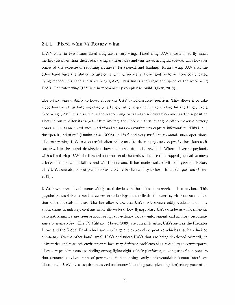
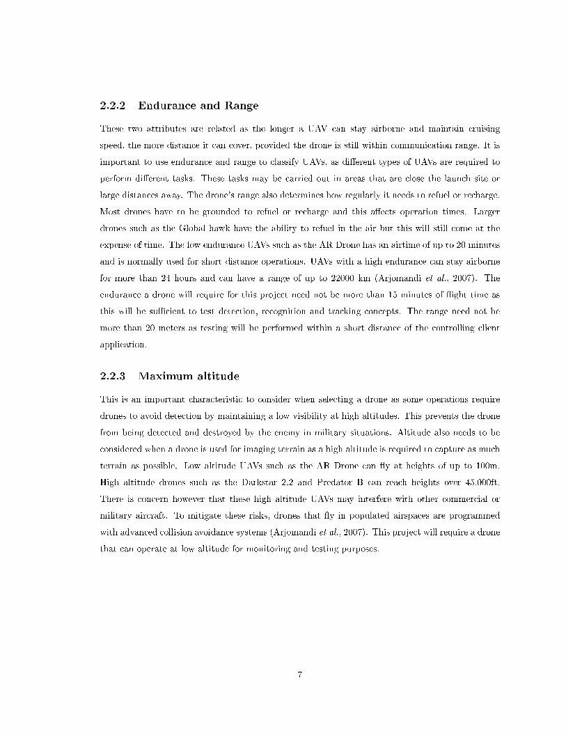
UAVs can range drastically in weight from the micro UAVs that can weigh up to 5kgs such as
the Dragon Eye in Figure 2.1 to the huge Globo Hawk which weighs over 11 tonnes. The lighter
UAVs tend to make use of electric motors whereas the heavier UAVs use turbo fan or jet engines
(Arjomandi et al., 2007). This project requires a light weight drone that can be operated indoors
for testing purposes.
Figure 2.1: The Dragon Eye. A micro UAV (Arjomandi et al., 2007)
6
2.2.2 Endurance and Range
These two attributes are related as the longer a UAV can stay airborne and maintain cruising
speed, the more distance it can cover, provided the drone is still within communication range. It is
important to use endurance and range to classify UAVs, as di�erent types of UAVs are required to
perform di�erent tasks. These tasks may be carried out in areas that are close the launch site or
large distances away. The drone's range also determines how regularly it needs to refuel or recharge.
Most drones have to be grounded to refuel or recharge and this a�ects operation times. Larger
drones such as the Global hawk have the ability to refuel in the air but this will still come at the
expense of time. The low endurance UAVs such as the AR Drone has an airtime of up to 20 minutes
and is normally used for short distance operations. UAVs with a high endurance can stay airborne
for more than 24 hours and can have a range of up to 22000 km (Arjomandi et al., 2007). The
endurance a drone will require for this project need not be more than 15 minutes of �ight time as
this will be su�cient to test detection, recognition and tracking concepts. The range need not be
more than 20 meters as testing will be performed within a short distance of the controlling client
application.
2.2.3 Maximum altitude
This is an important characteristic to consider when selecting a drone as some operations require
drones to avoid detection by maintaining a low visibility at high altitudes. This prevents the drone
from being detected and destroyed by the enemy in military situations. Altitude also needs to be
considered when a drone is used for imaging terrain as a high altitude is required to capture as much
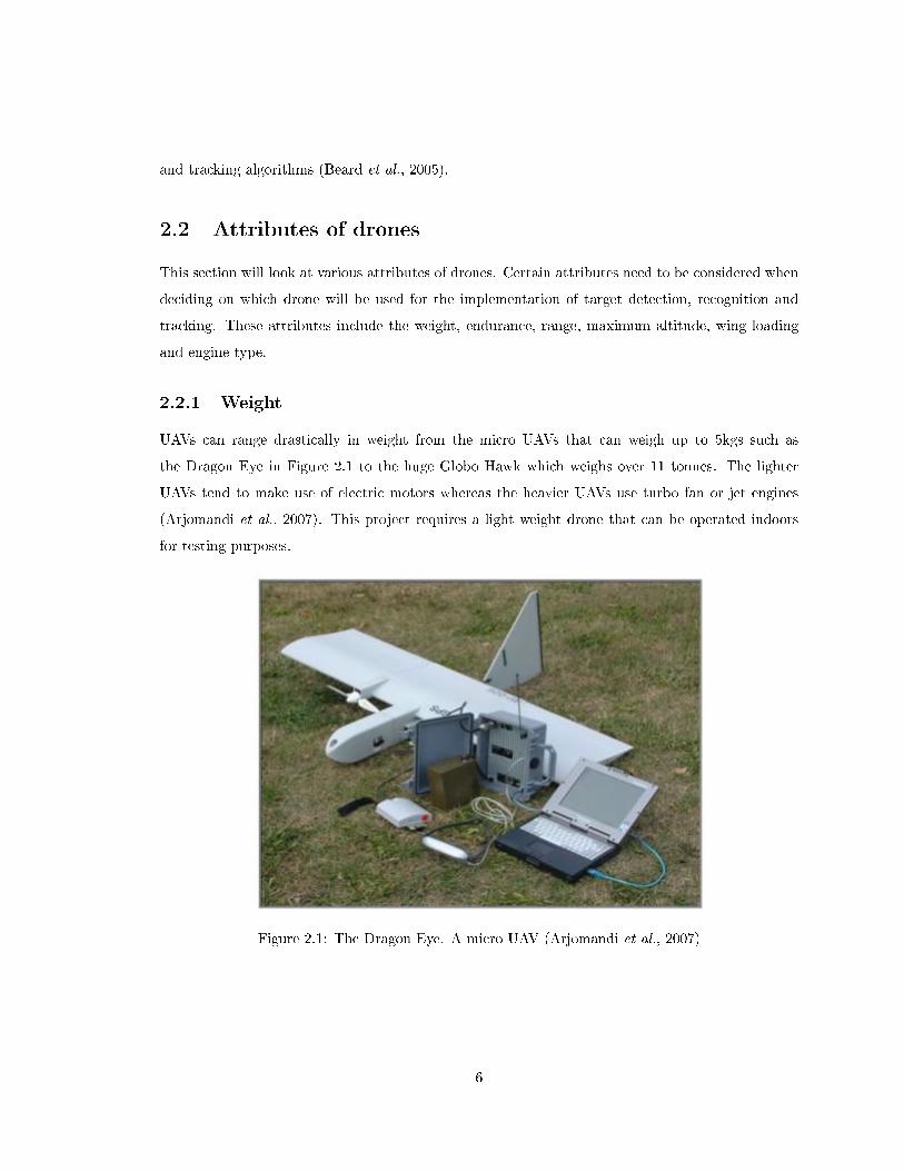
terrain as possible. Low altitude UAVs such as the AR Drone can �y at heights of up to 100m.
High altitude drones such as the Darkstar 2.2 and Predator B can reach heights over 45,000ft.
There is concern however that these high altitude UAVs may interfere with other commercial or
military aircraft. To mitigate these risks, drones that �y in populated airspaces are programmed
with advanced collision avoidance systems (Arjomandi et al., 2007). This project will require a drone
that can operate at low altitude for monitoring and testing purposes.
7
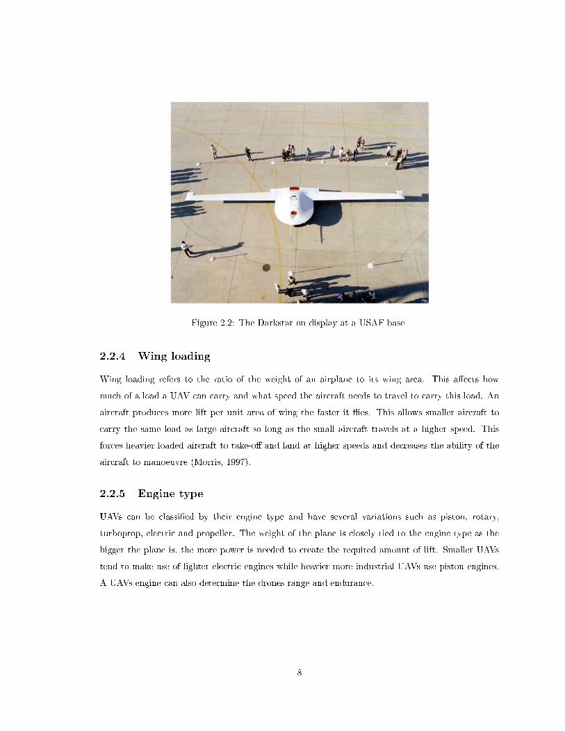
Figure 2.2: The Darkstar on display at a USAF base
2.2.4 Wing loading
Wing loading refers to the ratio of the weight of an airplane to its wing area. This a�ects how
much of a load a UAV can carry and what speed the aircraft needs to travel to carry this load. An
aircraft produces more lift per unit area of wing the faster it �ies. This allows smaller aircraft to
carry the same load as large aircraft so long as the small aircraft travels at a higher speed. This
forces heavier loaded aircraft to take-o� and land at higher speeds and decreases the ability of the
aircraft to manoeuvre (Morris, 1997).
2.2.5 Engine type
UAVs can be classi�ed by their engine type and have several variations such as piston, rotary,
turboprop, electric and propeller. The weight of the plane is closely tied to the engine type as the
bigger the plane is, the more power is needed to create the required amount of lift. Smaller UAVs
tend to make use of lighter electric engines while heavier more industrial UAVs use piston engines.
A UAVs engine can also determine the drones range and endurance.
8
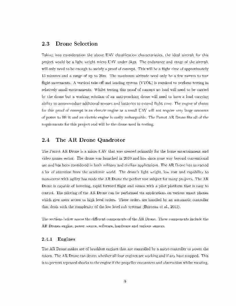
2.3 Drone Selection
Taking into consideration the above UAV classi�cation characteristics, the ideal aircraft for this
project would be a light weight micro UAV under 5kgs. The endurance and range of the aircraft
will only need to be enough to satisfy a proof of concept. This will be a �ight time of approximately
15 minutes and a range of up to 20m. The maximum altitude need only be a few metres to test
�ight movements. A vertical take-o� and landing system (VTOL) is required to perform testing in
relatively small environments. Whilst testing this proof of concept no load will need to be carried
by the drone but a working solution of an anti-poaching drone will need to have a load carrying
ability to accommodate additional sensors and batteries to extend �ight time. The engine of choice
for this proof of concept is an electric engine as a small UAV will not require very large amounts
of power to lift it and an electric engine is easily rechargeable. The Parrot AR Drone �ts all of the
requirements for this project and will be the drone used in testing.
2.4 The AR Drone Quadrotor
The Parrot AR Drone is a micro UAV that was created primarily for the home entertainment and
video games sector. The drone was launched in 2010 and has since gone way beyond conventional
use and has been considered in both military and civilian applications. The AR Drone has attracted
a lot of attention from the academic world. The drone's light weight, low cost and capability to
manoeuvre with agility has made the AR Drone the perfect test subject for many projects. The AR
Drone is capable of hovering, rapid forward �ight and comes with a pilot platform that is easy to
control. The piloting of the AR Drone can be performed via applications on various smart phones
which give users access to high level orders. These orders are handled by an automatic controller
that deals with the complexity of the low level sub systems (Bristeau et al., 2011).
The sections below assess the di�erent components of the AR Drone. These components include the
AR Drones engine, power source, software, hardware and various sensors.
2.4.1 Engines
The AR Drone makes use of brushless engines that are controlled by a micro controller to power the
rotors. The AR Drone can detect whether all four engines are working and if any have stopped. This
is to prevent repeated shocks to the engine if the propeller encounters and obstruction whilst rotating.
9
If an obstruction to any propeller is detected, the AR Drone stops all engines (Stephane Piskorski,
2011).
2.4.2 LiPo batteries
The AR Drone makes use of a charged 100mAh, 11.1V LiPo battery to �y. The battery's charge is
determined full when at 12.5V and low when at 9V. The drone monitors the voltage of the battery
and displays it to the user as a percentage so that �ight decisions can be made accordingly. When
the drone detects the battery is at a low voltage, it sends a warning message to the user before
landing automatically. Should the voltage of the battery reach a critical point at any stage, the AR
Drone will shut down immediately to prevent the drone from behaving in any unexpected fashion
(Stephane Piskorski, 2011).
2.4.3 Accelerometer, gyrometers and processors
The AR Drone's sensors are located below the central hull of the drone. The AR Drone has a six
degrees of freedom, micro electro-mechanical system (MEMS) based, miniaturized inertial measure-
ment unit (Stephane Piskorski, 2011). This measurement unit provides the drone's software with
pitch, roll and yaw measurements. The measurement unit also contains a three axis accelerometer,
a two axis roll and pitch gyro meter and a single axis yaw gyro meter (Dijkshoorn, 2012). The AR
Drone also has two cameras, a motherboard, which holds two processors and sonar. One of these
processors is used to gather data from I/Os. The other is used to run all the algorithms that the
drone needs to maintain �ight stability and process images (Bristeau et al., 2011). The accelerometer
is a BMA150 made by Bosch Sensortec. �The accelerometer outputs g-forces (acceleration relative
to free-fall) as a quantity of acceleration� (Dijkshoorn, 2012). This measurement is based on the
phenomenon that the observed weight of an object changes whilst that object is accelerating. The
MEMS accelerometer makes use of three plates on separate axes and can measure acceleration in
the direction of the axis. This ability of the accelerometer to measure gravity allows it to be used
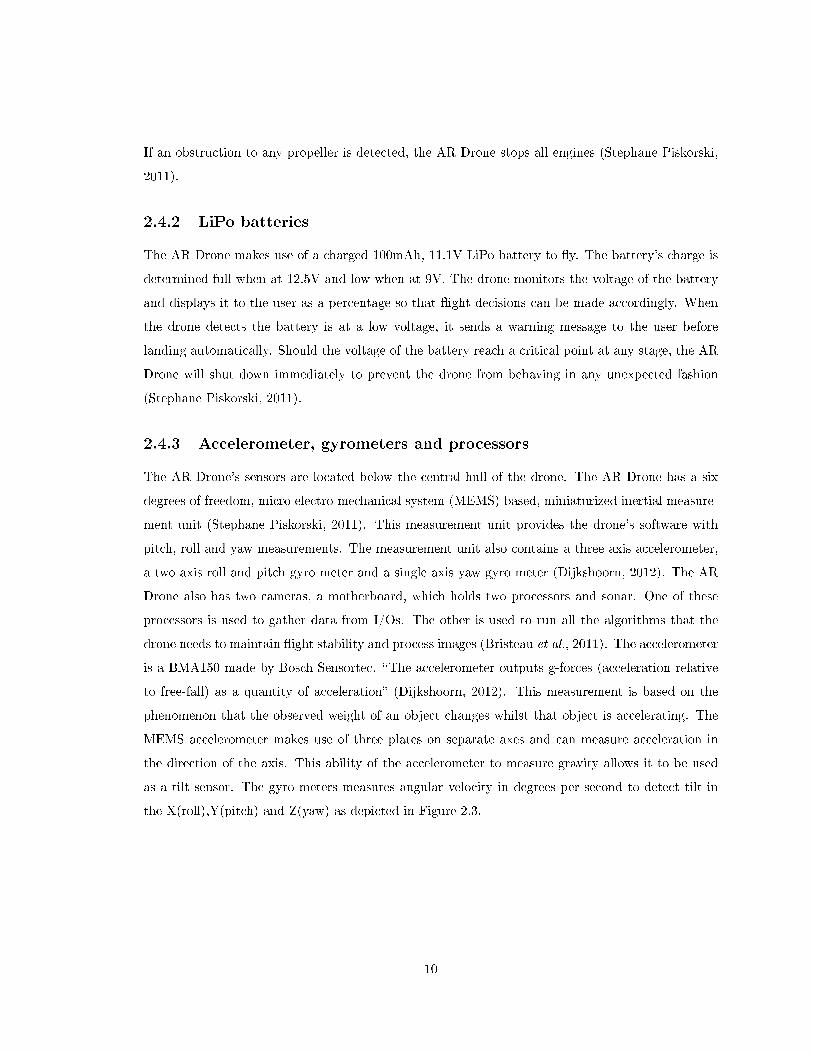
as a tilt sensor. The gyro meters measures angular velocity in degrees per second to detect tilt in
the X(roll),Y(pitch) and Z(yaw) as depicted in Figure 2.3.
10
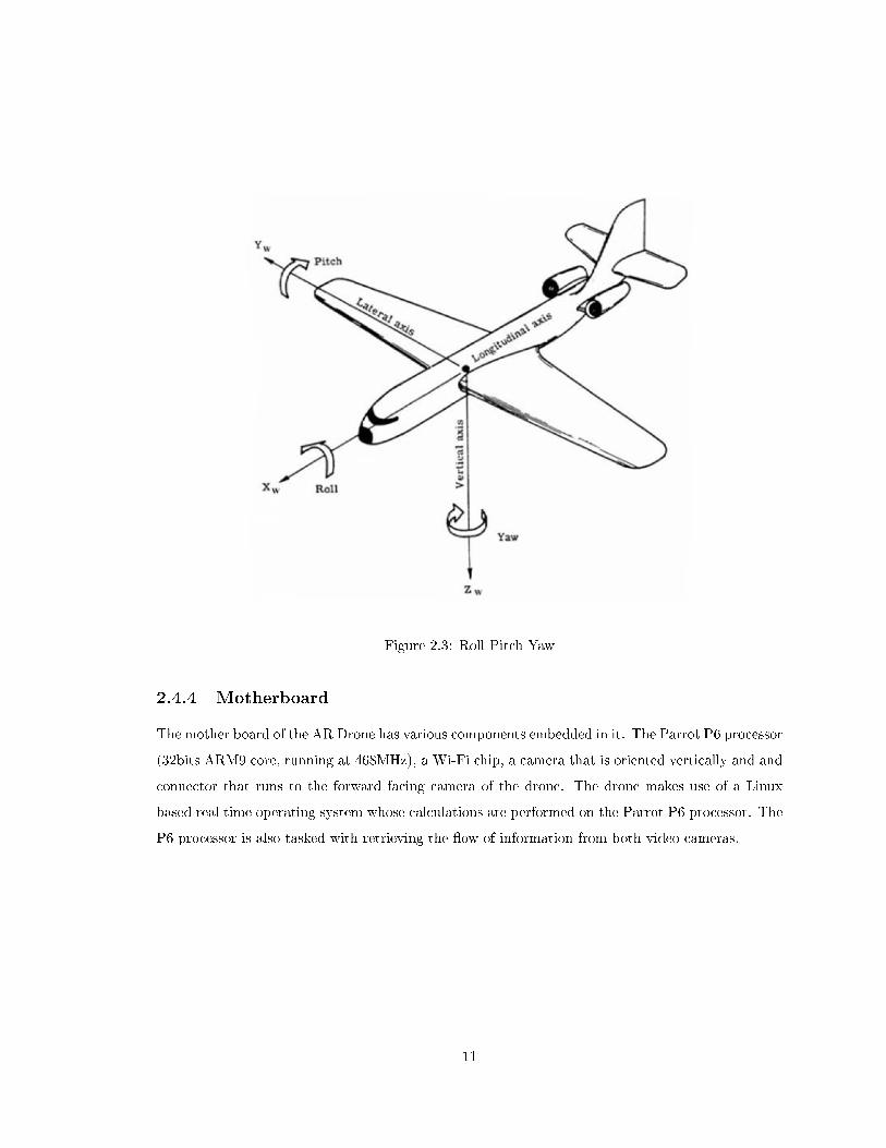
Figure 2.3: Roll Pitch Yaw
2.4.4 Motherboard
The mother board of the AR Drone has various components embedded in it. The Parrot P6 processor
(32bits ARM9 core, running at 468MHz), a Wi-Fi chip, a camera that is oriented vertically and and
connector that runs to the forward facing camera of the drone. The drone makes use of a Linux
based real time operating system whose calculations are performed on the Parrot P6 processor. The
P6 processor is also tasked with retrieving the �ow of information from both video cameras.
11
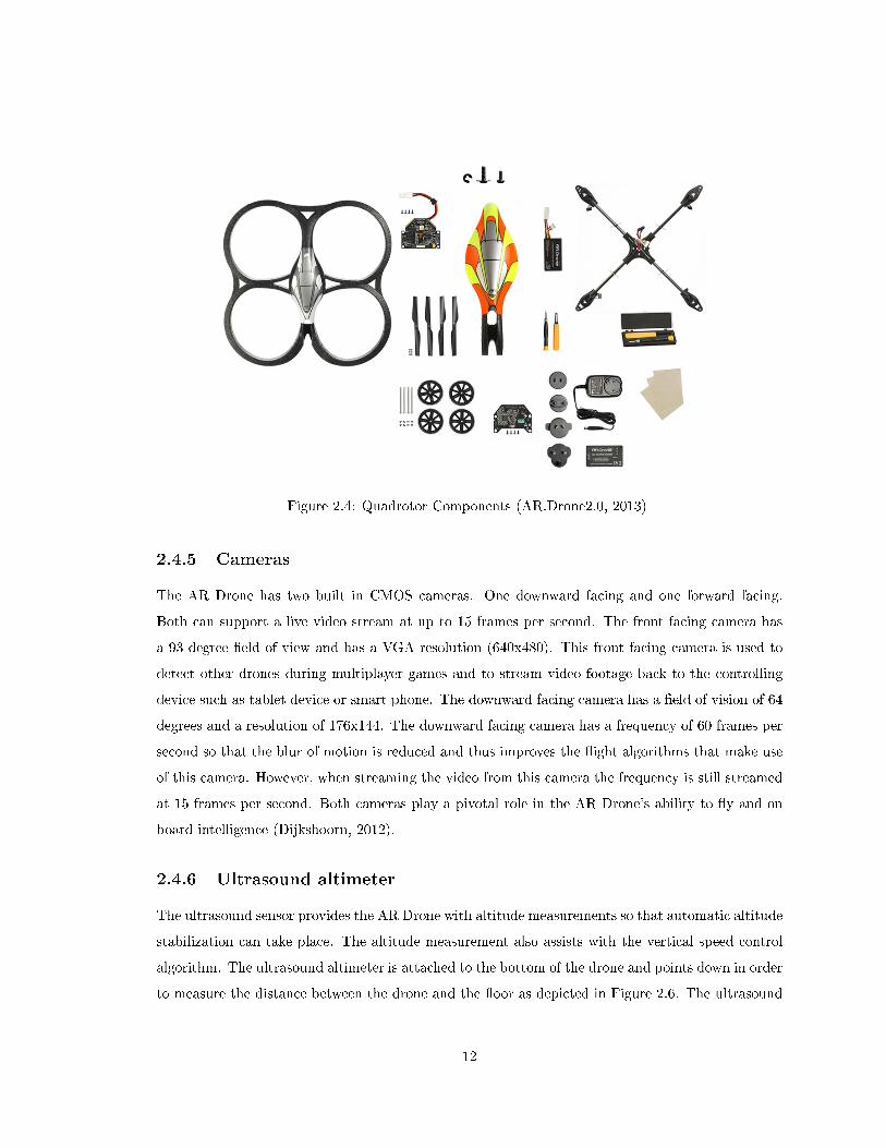
Figure 2.4: Quadrotor Components (AR.Drone2.0, 2013)
2.4.5 Cameras
The AR Drone has two built in CMOS cameras. One downward facing and one forward facing.
Both can support a live video stream at up to 15 frames per second. The front facing camera has
a 93 degree �eld of view and has a VGA resolution (640x480). This front facing camera is used to
detect other drones during multiplayer games and to stream video footage back to the controlling
device such as tablet device or smart phone. The downward facing camera has a �eld of vision of 64
degrees and a resolution of 176x144. The downward facing camera has a frequency of 60 frames per
second so that the blur of motion is reduced and thus improves the �ight algorithms that make use
of this camera. However, when streaming the video from this camera the frequency is still streamed
at 15 frames per second. Both cameras play a pivotal role in the AR Drone's ability to �y and on
board intelligence (Dijkshoorn, 2012).
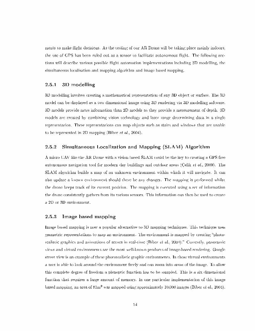
2.4.6 Ultrasound altimeter
The ultrasound sensor provides the AR Drone with altitude measurements so that automatic altitude
stabilization can take place. The altitude measurement also assists with the vertical speed control
algorithm. The ultrasound altimeter is attached to the bottom of the drone and points down in order
to measure the distance between the drone and the �oor as depicted in Figure 2.6. The ultrasound
12
waits for its transmitted signal to echo back to it and then determines the distance between the
object and the sensor using the amount of time it took the echo to return. The distance is computed
using the speed of sound where c ≈ 343m/s is the speed of sound in air.
Figure 2.5: Calcualting distance using the speed of sound (Dijkshoorn, 2012)
Figure 2.6: Ultrasound altimeter (Stephane Piskorski, 2011)
2.4.7 Embedded software
The operating system (OS) that the AR Drone uses is a custom embedded Linux real time OS. The
OS simultaneously manages threads pertaining to: �Wi-Fi communications, video data sampling,
video compression (for wireless transmission), image processing, sensors acquisition, state estimation
and closed-loop control� (Bristeau et al., 2011).
2.5 Flight Automation
Introduction
Flight automation is an important factor to consider when implementing a target detection, recogni-
tion and tracking system. Automation will allow a drone to execute various directives when human
control is not available.
Flight automation using the AR Drone can be performed by using the images from the cameras to
implement computer vision control, create three dimensional (3D) models or use sensor measure-
13
ments to make �ight decisions. As the testing of our AR Drone will be taking place mainly indoors,
the use of GPS has been ruled out as a sensor to facilitate autonomous �ight. The following sec-
tions will describe various possible �ight automation implementations including 3D modelling, the
simultaneous localisation and mapping algorithm and image based mapping.
2.5.1 3D modelling
3D modelling involves creating a mathematical representation of any 3D object or surface. The 3D
model can be displayed as a two dimensional image using 3D rendering via 3D modelling software.
3D models provide more information than 2D models as they provide a measurement of depth. 3D
models are created by combining vision technology and laser range determining data in a single
representation. These representations can map objects such as stairs and windows that are unable
to be represented in 2D mapping (Biber et al., 2004).
2.5.2 Simultaneous Localization and Mapping (SLAM) Algorithm
A micro UAV like the AR Drone with a vision based SLAM could be the key to creating a GPS free
autonomous navigation tool for modern day buildings and outdoor areas (Çelik et al., 2009). The
SLAM algorithm builds a map of an unknown environment within which it will navigate. It can
also update a known environment should there be any changes. The mapping is performed whilst
the drone keeps track of its current position. The mapping is executed using a set of information
the drone consistently gathers from its various sensors. This information can then be used to create
a 2D or 3D environment.
2.5.3 Image based mapping
Image based mapping is now a popular alternative to 3D mapping techniques. This technique uses
geometric representations to map an environment. The environment is mapped by creating �photo-
realistic graphics and animations of scenes in real-time (Biber et al., 2004).� Currently, panoramic
views and virtual environments are the most well-known products of image-based rendering. Google
street view is an example of these photorealistic graphic environments. In these virtual environments
a user is able to look around the environment freely and can zoom into areas of the image. To allow
this complete degree of freedom a plenoptic function has to be sampled. This is a six dimensional
function that requires a large amount of memory. In one particular implementation of this image
based mapping, an area of 81m² was mapped using approximately 10,000 images (Biber et al., 2004).
14
Summary
After considering the above �ight automation implementations as well as the capabilities of the AR
Drone it was decided to use an image based approach to automation. The AR Drone's on board
camera will be used to gather images which will be processed to make �ight decision.
2.5.4 Related work in visual and non-visual �ight automation
This section covers related work in the �eld of �ight automation and mapping. The sections include
visual based navigation, non-visual based navigation, stability and control and navigation patterns.
Introduction
It is necessary to consider related work in visual and non-visual �ight automation so that informed
decisions can be made when implementing the navigation of the AR Drone. Related work also
illustrates the capabilities of the UAVs and can highlight the importance of certain aspects of �ight
navigation automation.
2.5.5 Visual based navigation
Using micro UAVs that use image based navigation techniques is an e�cient navigation technique.
This is because a vision based navigation system can provide long range sensing with low power
demands. The study by Nicoud et al. (2002) discusses UAV design trade-o�s for indoor aerial
vehicles (Nicoud & Zu�erey, 2002). These trade-o�s address the issues of aerodynamics, the weights
of UAVs, wing, propeller and motor characteristics. The paper proposes a methodology to optimize
the motor/gear/propeller system from which a UAV with low power demands is created. Mejias et
al. (2006) used a vision based navigation system to land a UAV whilst avoiding power lines (Mejias
et al., 2006). The vision system here allows the UAV to make �ight decisions based on its 2D position
in relation to a feature or set of features in the image. The features used here were those of power
lines and their various arrangements. Zingg et al. (2011) discuss a vision based algorithm for �ying
a micro UAV in corridors using a depth map (Zingg et al., 2010) (Bills et al., 2011). This approach
uses the optical �ow of images from cameras mounted on the UAV to avoid collisions.
2.5.6 Non-visual based navigation
Non-visual navigation methods make use of sensors such as laser range scanners, sonar and infra-red.
The study by Roberts et al. (2009) made use of ultra-sonic and infra-red sensors to �y a quadrotor
15
in an environment where strict requirements needed to be ful�lled (Roberts et al., 2009). This
paper proved it viable for a small, lightweight, large range UAV with infra-red sensors to be able to
navigate e�ectively in circumstances of tilting, misalignment and ambient light changes. It was able
to overcome these conditions whilst still maintaining range and directional accuracy in the 6x7m
environment in which tests were performed. This implementation however could not perform long
range sensing beyond these dimensions. The study by Achtelik et al. (2009) used a laser range�nder
and a stereo camera to implement navigation in unstructured and unknown indoor environments
using a quadrotor (Achtelik et al., 2009). These sensors are e�ective in determining the helicopter's
relative motion and velocity. The number of sensors that a quadrotor can use is limited by the
payload the UAV can carry. This restricts the capability of UAVs and custom quadrotors are often
built to handle a heavy load of sensors or additional batteries for those that are power demanding.
Most micro UAVs only have the ability to carry small payloads and power e�cient sensors like a
camera (Bills et al., 2011).
2.5.7 Stabililty and control
Vision based algorithms have been used for �ight stabilisation and the pose estimation of UAVs.
Some implementations of these stabilisation algorithms make use of specialised cameras that �can
be used to refocus at certain depths� (Bills et al., 2011). This will allow the drone to maintain a
certain distance from speci�c visual elements. The study by Moore et al. (2009) made use of this
concept where two UAV mounted cameras are used to obtain stereo information on the UAV's height
above the ground and the distance to potential objects (Moore et al., 2009). This camera-mirror
system uses specially shaped re�ective surfaces that are associated with each camera to �map out
a collision-free cylinder through which the aircraft can pass without encountering objects� (Moore
et al., 2009). This method of vision control is particularly e�ective for terrain following and object
avoidance. The study by Johnson (2008) used vision based algorithms to make a quadrotor hover
with attitude stabilization and position control using ��rst principles and a proportional-derivative
control method� (Johnson, 2008). Additional studies that address the issue of stabilisation of a
quadrotor include Kendoul et al. (2009) and Cherian et al. (2009) (Kendoul et al., 2009) (Cherian
et al., 2009). Kendoul et al. (2009) make use of a low-resolution on board camera and an Inertial
Measurement Unit (IMU) to estimate optic �ow, UAV motion and depth mapping. Cherian et al.
(2009) proposed a new algorithm to estimate UAV altitude by using images taken from the downward
facing camera of the UAV (Cherian et al., 2009). This algorithm would use texture information of
the image from the downward facing camera and to determine the altitude of the UAV.
16
2.5.8 Navigation patterns
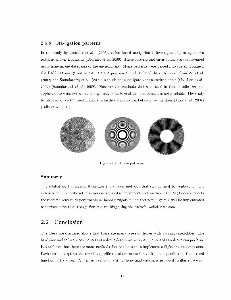
In the study by Tournier et al. (2006), vision based navigation is investigated by using known
patterns and environments (Tournier et al., 2006). These patterns and environments are represented
using large image databases of the environment. Moire patterns were pasted into the environment
the UAV was navigating to estimate the position and altitude of the quadrotor. Courbon et al.
(2009) and Soundararaj et al. (2009) used vision to navigate known environments (Courbon et al.,
2009) (Soundararaj et al., 2009). However the methods that were used in these studies are not
applicable to scenarios where a large image database of the environment is not available. The study
by Mori et al. (2007) used markers to facilitate navigation between two markers (Mori et al., 2007)
(Bills et al., 2011).
Figure 2.7: Moire patterns
Summary
The related work discussed illustrates the various methods that can be used to implement �ight
automation. A speci�c set of sensors is required to implement each method. The AR Drone supports
the required sensors to perform visual based navigation and therefore a system will be implemented
to perform detection, recognition and tracking using the drone's available sensors.
2.6 Conclusion
The literature discussed shows that there are many types of drones with varying capabilities. The
hardware and software components of a drone determine various functions that a drone can perform.
It also shows that there are many methods that can be used to implement a �ight navigation system.
Each method requires the use of a speci�c set of sensors and algorithms, depending on the desired
function of the drone. A brief overview of existing drone applications is provided to illustrate some
17

drone capabilities. This serves to indicate the di�erences, advantages and disadvantages of drones
and their applications. This background information served as a basis upon which a drone was
chosen to implement a detection, recognition and tracking system. It also helped in choosing the
tools and algorithms that are used to implement this system.
18
Chapter 3
Application Programming Interfaces
(APIs)
Introduction
To create a system to perform target detection, recognition and tracking various software develop-
ment environments and tools need to be considered. Existing code libraries and integrated devel-
opment environments will assist with the programming of, and interfacing with, the drone. The
following sections describe the various APIs that were explored to determine which was best suited
to carry out target recognition and tracking. This chapter will look at the Parrot AR Drone Software
Development Kit (SDK) 2.0.1, EZ-Builder (EZ-B) generic robotics SDK and the AC Drone.
3.1 Parrot AR Drone SDK 2.0.1
The AR Drone has an open source API that is widely used as a research standard for developing
AR Drone applications. The API available at (AR.Drone, 2009) includes a software development
kit (SDK) that has been written in C and runs on iOS, Android and Linux platforms. The API
does not however give the developer access to software that is embedded on the drone. There
are four components, also called communication services that are implemented in the SDK. These
components provide information on the state of the drone and allow the user to control and con�gure
the drone. These communication services are AT Commands, Navigation Data, video stream and
the control port.
19
3.2 AT Commands
AT commands are used to send commands and con�guration requests to the AR Drone. The
command syntax is as follows:
�AT*PCMD=<sequence_number>,<�ag>,<roll_p>,<pitch_p>,<gaz_p>,<rot_p>�
Sequence number refers to the command's turn for execution. This number depends on the number
of commands that have come before it (Portal, 2011). The �ag argument de�nes whether the drone
will look at the arguments that follow it. When the �ag is 1 (True) the AR Drone will look at the
arguments roll, pitch, gaz and rotation. When the �ag is set to 0 (False), the drone will perform the
�hover� command and attempt to maintain the same position using algorithms to cancel the inertial
speed of the drone. Each argument is explained below. Refer to Figure 2.3 for an illustration of the
movement direction.
3.2.1 Roll argument
The argument roll_p is a double value that can be set in the range [-1..1]. This value represents
a �percentage of the max value of the angle roll that the drone can achieve.� (Portal, 2011) The
maximum amount of roll that the drone can achieve is hard coded at 12 degrees. To illustrate this,
if we set roll_p at 0.5 the AR Drone will shift 6 degrees in the roll angle which will cause the drone
to move to the right. The drone will perform the opposite when roll_p is set to -0.5.
3.2.2 Pitch argument
The argument pitch_p is also double value that can be set in the range [-1..1]. This value represents
a �percentage of the max value of the angle pitch that the drone can achieve.� (Portal, 2011) The
maximum amount of pitch that the drone can achieve is hard coded at 12 degrees. To illustrate this,
if we set pitch_p at 0.5 the AR Drone will shift 6 degrees in the pitch angle which will cause the
drone to move to the backwards. The drone will perform the opposite when pitch_p is set to -0.5.
3.2.3 Gaz argument
The argument gaz_p is also double value that can be set in the range [-1..1]. This value represents
a �percentage of the max value of the vertical speed that the drone can achieve.� (Portal, 2011) The
20
maximum vertical speed that the drone can achieve is hard coded at 0.7m/s. To illustrate this, if
we set gaz_p at 0.5 the AR Drone will travel on the Z axis with a speed of 0.35m/s which is the
upward movement of the drone. The drone will perform the opposite when gaz_p is set to -0.5.
3.2.4 Rotation argument
The argument rot_p is also double value that can be set in the range [-1..1]. This value represents
a �percentage of the max value of the angular speed that the drone can achieve.� (Portal, 2011) The
maximum angular speed that the drone can achieve is set at a default of 100 degrees. To illustrate
this, if we set rot_p at 0.5 the AR Drone will turn right at an angle of 50 degrees. The drone will
perform the opposite when rot_p is set to -0.5.
Summary
These commands make it easy for the user to control the drone. If the user wants the drone to hover,
an AT Command with a �ag value of 1 should be set and all the other arguments set to 0. The
drone will produce a standard amount of lift and not move from its position but will slide a little
due to inertia. The drone has a built in algorithm to cancel inertia that can be employed by sending
an AT Command with just the �ag value set to 0. The algorithm makes use of the downward facing
camera to attempt to stay above the same spot. This is called the �hover� procedure (Portal, 2011).
By setting values for the last four arguments the user can make the drone perform complex �ight
patterns for example the command:
�AT*PCMB=<1>,<1>,<0.25>,<0.25>,<0.5>,<0.25>� will make the drone roll 3 de-
grees to the right, go backwards at an angle of 3 degrees, rotate to the left and ascend at 0.35m\s.
3.3 Navigation Data
The Navigation Data communication service provides the API with all the information pertaining
to the state of the drone such as the drone's altitude, speed and attitude. NavData also returns raw
measurements taken from the Drones sensors. This NavData is sent to the client side API by the
drone 200 times per second and 30 times a second when in demo mode.
21
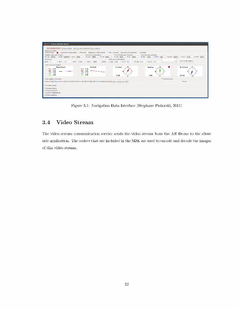
Figure 3.1: Navigation Data Interface (Stephane Piskorski, 2011)
3.4 Video Stream
The video stream communication service sends the video stream from the AR Drone to the client
side application. The codecs that are included in the SDK are used to encode and decode the images
of this video stream.
22
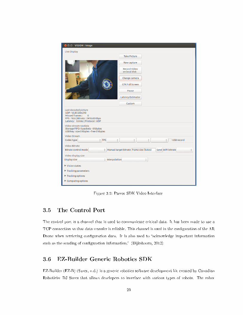
Figure 3.2: Parrot SDK Video Interface
3.5 The Control Port
The control port is a channel that is used to communicate critical data. It has been made to use a
TCP connection so that data transfer is reliable. This channel is used in the con�guration of the AR
Drone when retrieving con�guration data. It is also used to �acknowledge important information
such as the sending of con�guration information.� (Dijkshoorn, 2012)
3.6 EZ-Builder Generic Robotics SDK
EZ-Builder (EZ-B) (Sures, n.d.) is a generic robotics software development kit created by Canadian
Roboticist DJ Sures that allows developers to interface with various types of robots. The robot
23

Figure 3.3: Layered architecture of a client application built upon the Parrot AR Drone SDK(Dijkshoorn, 2012)
control software has a GUI interface as well as a C#, VB and C++ programming environment.
Using EZ-B, various tracking algorithms were implemented by exporting the video feed to OpenCV
for image processing. This processed image was then sent back to EZ-B for the execution of various
tracking directives and scripts such as velocity tracking and search algorithms.
3.6.1 Video Interface
The EZ-B initiates a link to the AR Drones video stream. This stream can then be a�ected using
OpenCV functions to enhance the quality of the image. Image brightness, contrast and saturation
can be adjusted from this interface. The pixel density of the stream can also be swapped between
640x480 and 320x240. This interface also allows one to record the video stream to �le.
24
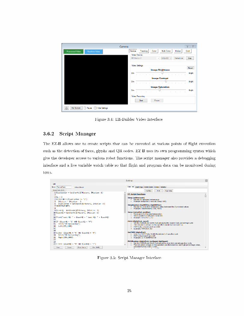
Figure 3.4: EZ-Builder Video Interface
3.6.2 Script Manager
The EZ-B allows one to create scripts that can be executed at various points of �ight execution
such as the detection of faces, glyphs and QR codes. EZ-B uses its own programming syntax which
give the developer access to various robot functions. The script manager also provides a debugging
interface and a live variable watch table so that �ight and program data can be monitored during
tests.
Figure 3.5: Script Manager Interface
25
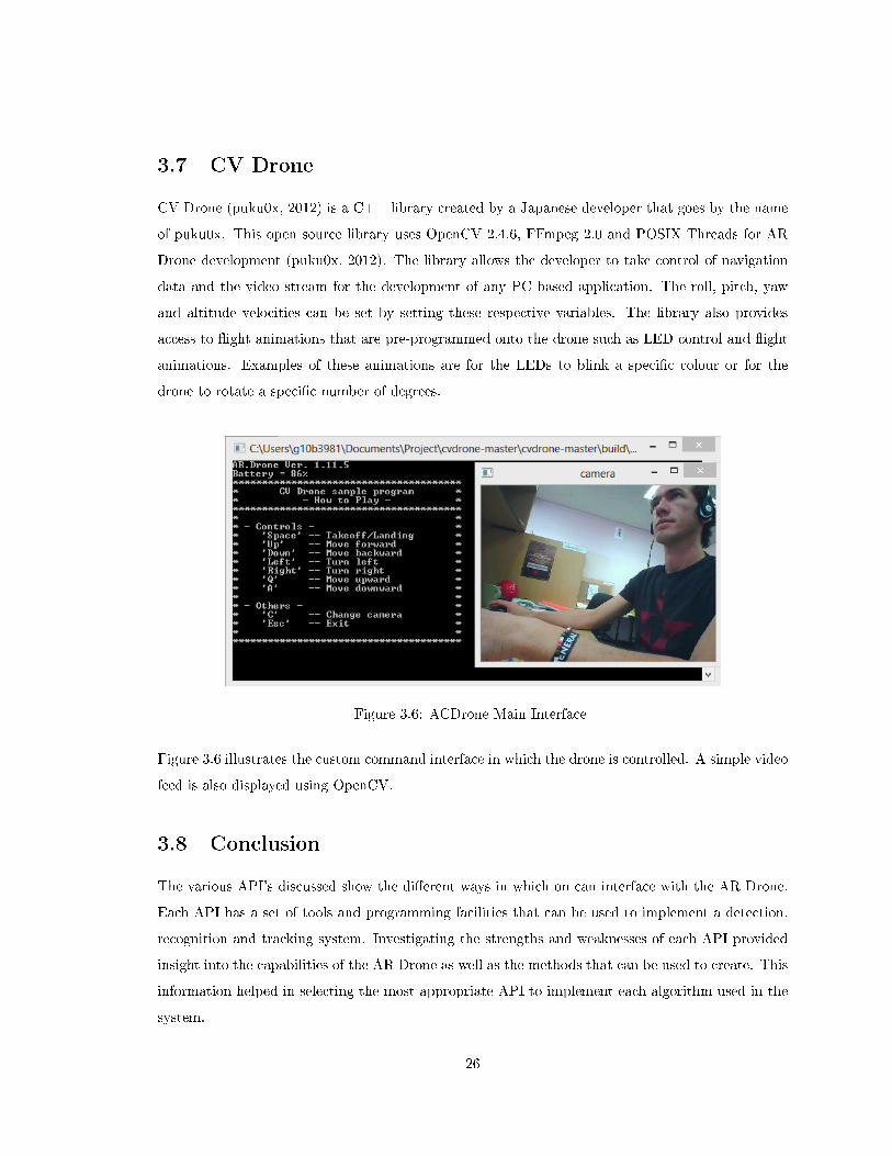
3.7 CV Drone
CV Drone (puku0x, 2012) is a C++ library created by a Japanese developer that goes by the name
of puku0x. This open source library uses OpenCV 2.4.6, FFmpeg 2.0 and POSIX Threads for AR
Drone development (puku0x, 2012). The library allows the developer to take control of navigation
data and the video stream for the development of any PC based application. The roll, pitch, yaw
and altitude velocities can be set by setting these respective variables. The library also provides
access to �ight animations that are pre-programmed onto the drone such as LED control and �ight
animations. Examples of these animations are for the LEDs to blink a speci�c colour or for the
drone to rotate a speci�c number of degrees.
Figure 3.6: ACDrone Main Interface
Figure 3.6 illustrates the custom command interface in which the drone is controlled. A simple video
feed is also displayed using OpenCV.
3.8 Conclusion
The various API's discussed show the di�erent ways in which on can interface with the AR Drone.
Each API has a set of tools and programming facilities that can be used to implement a detection,
recognition and tracking system. Investigating the strengths and weaknesses of each API provided
insight into the capabilities of the AR Drone as well as the methods that can be used to create. This
information helped in selecting the most appropriate API to implement each algorithm used in the
system.
26
Chapter 4
Design and Tools
This chapter describes the software tools and algorithms used to perform detection, tracking and
recognition functions.
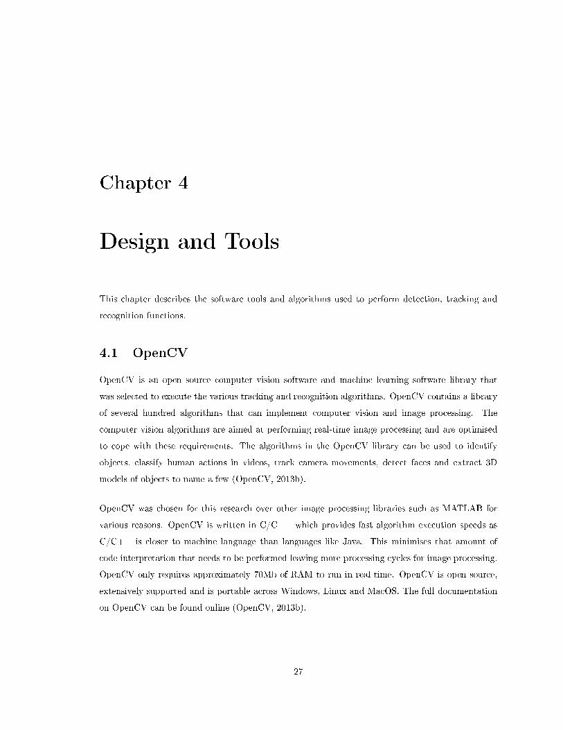
4.1 OpenCV
OpenCV is an open source computer vision software and machine learning software library that
was selected to execute the various tracking and recognition algorithms. OpenCV contains a library
of several hundred algorithms that can implement computer vision and image processing. The
computer vision algorithms are aimed at performing real-time image processing and are optimised
to cope with these requirements. The algorithms in the OpenCV library can be used to identify
objects, classify human actions in videos, track camera movements, detect faces and extract 3D
models of objects to name a few (OpenCV, 2013b).
OpenCV was chosen for this research over other image processing libraries such as MATLAB for
various reasons. OpenCV is written in C/C++ which provides fast algorithm execution speeds as
C/C++ is closer to machine language than languages like Java. This minimises that amount of
code interpretation that needs to be performed leaving more processing cycles for image processing.
OpenCV only requires approximately 70Mb of RAM to run in real-time. OpenCV is open source,
extensively supported and is portable across Windows, Linux and MacOS. The full documentation
on OpenCV can be found online (OpenCV, 2013b).
27
4.2 CamShift algorithm
CamShift stands for Continuously Adaptive Mean Shift as this algorithm is based on the Mean
Shift algorithm. CamShift is commonly used as an object tracking tool and is used as one method
of tracking objects and faces in OpenCV. It combines the Mean Shift algorithm with an adaptive
region-sizing step. CamShift is able to handle dynamic distributions as it can adjust its search
window size for the next image frame based on the zeroth moment of the current frames distribution
(Isaac Gerg, 2003).
Mean Shift Algorithm
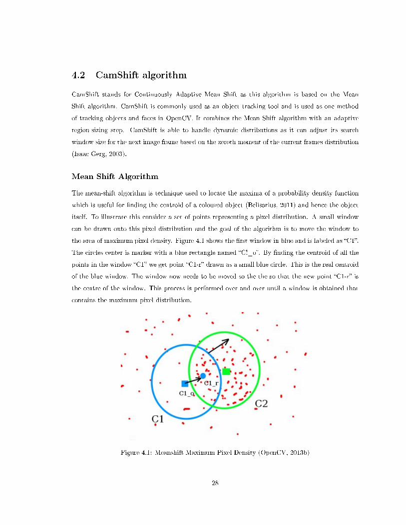
The mean-shift algorithm is technique used to locate the maxima of a probability density function
which is useful for �nding the centroid of a coloured object (Belisarius, 2011) and hence the object
itself. To illustrate this consider a set of points representing a pixel distribution. A small window
can be drawn onto this pixel distribution and the goal of the algorithm is to move the window to
the area of maximum pixel density. Figure 4.1 shows the �rst window in blue and is labeled as �C1�.
The circles center is marker with a blue rectangle named �C!_o�. By �nding the centroid of all the
points in the window �C1� we get point �C1-r� drawn as a small blue circle. This is the real centroid
of the blue window. The window now needs to be moved so the the so that the new point �C1-r� is
the centre of the window. This process is performed over and over until a window is obtained that
contains the maximum pixel distribution.
Figure 4.1: Meanshift Maximum Pixel Density (OpenCV, 2013b)
28
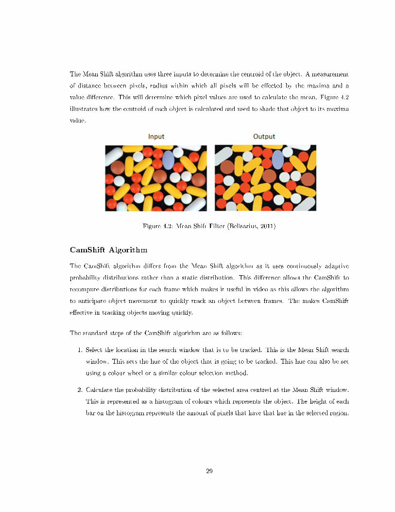
The Mean Shift algorithm uses three inputs to determine the centroid of the object. A measurement
of distance between pixels, radius within which all pixels will be e�ected by the maxima and a
value di�erence. This will determine which pixel values are used to calculate the mean. Figure 4.2
illustrates how the centroid of each object is calculated and used to shade that object to its maxima
value.
Figure 4.2: Mean Shift Filter (Belisarius, 2011)
CamShift Algorithm
The CamShift algorithm di�ers from the Mean Shift algorithm as it uses continuously adaptive
probability distributions rather than a static distribution. This di�erence allows the CamShift to
recompute distributions for each frame which makes it useful in video as this allows the algorithm
to anticipate object movement to quickly track an object between frames. The makes CamShift
e�ective in tracking objects moving quickly.
The standard steps of the CamShift algorithm are as follows:
1. Select the location in the search window that is to be tracked. This is the Mean Shift search
window. This sets the hue of the object that is going to be tracked. This hue can also be set
using a colour wheel or a similar colour selection method.
2. Calculate the probability distribution of the selected area centred at the Mean Shift window.
This is represented as a histogram of colours which represents the object. The height of each
bar on the histogram represents the amount of pixels that have that hue in the selected region.
29
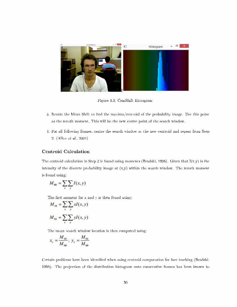
Figure 4.3: CamShift Histogram
3. Iterate the Mean Shift to �nd the maxima/centroid of the probability image. Use this point
as the zeroth moment. This will be the new centre point of the search window.
4. For all following frames, centre the search window at the new centroid and repeat from Step
2. (Allen et al., 2004)
Centroid Calculation
The centroid calculation in Step 2 is found using moments (Bradski, 1998). Given that I(x,y) is the
intensity of the discrete probability image at (x,y) within the search window. The zeroth moment
is found using:
The �rst moment for x and y is then found using:
The mean search window location is then computed using:
Certain problems have been identi�ed when using centroid computation for face tracking (Bradski,
1998). The projection of the distribution histogram onto consecutive frames has been known to
30
introduce a bias in the target location estimate (Allen et al., 2004).
Glyph Recognition
Once a glyph has been found it can be extracted from the main image using Quadrilateral Trans-
formation. This transforms any quadrilateral from an image into a rectangular image. Many glyph
images that are detected will be at various angles and depths and so quadrilateral transformation
serves to standardise the image to be input to the glyph recognition algorithm.
Using the transformed glyph image we can perform glyph recognition. This can be performed in
various ways such as shape recognition or template matching. As the glyph is divided up into rows
and columns when it is constructed, these rows and columns can be remapped to the transformed
image to determine individual cell colours. After remapping the cells to the image, every white and
black pixel in the cell can be counted to determine to original colour of the cell. Whichever colour
occurs most in each cell can be assumed to be the original colour of the entire cell. The ratio of black
to white pixels will also indicate a degree of certainty that can be used further when comparing the
glyph to known glyphs. The glyphs resulting colour can then be mapped to a matrix of 1's and 0's
that represent black and white respectively. This matrix can be used to match the glyph against
know glyph matrices. Known glyphs are stored in their binary matrix representation. Each black
square of the glyph represented as a 0 and each white square represented as a 1 as can be seen
in Figure 4.11. It is highly likely that a detected glyph may have been rotated in the image or
by quadrilateral transformation. This would cause the glyphs matrix representation to be di�erent
when reconstructed. This problem can solved by either storing all four matrix representations for
one glyph or by rotating the reconstructed glyph matrix. This matching process requires glyphs to
maintain a unique matrix representation for each rotation.
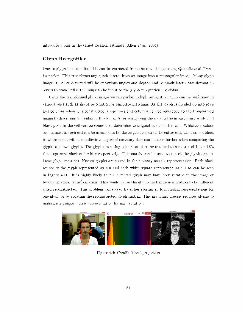
Figure 4.4: CamShift backprojection
31
4.3 Viola Jones
Viola Jones is a �machine learning approach for visual object detection which is capable of processing
images extremely rapidly and achieving high detection rates� (Viola et al., 2005). This section will
focus on Viola and Jones's contribution to object detection in the context of face detection. Their
contribution came in three parts.
1. Creation of a classi�er that was based upon a combination of weaker classi�ers using the
AdaBoost machine learning algorithm (Viola et al., 2005). These weak classi�ers represented
very simple features used to detect a face.
2. Viola and Jones created their own implementation of a standard algorithm to combine classi-
�ers to create new classi�ers. Although their algorithm could take time to detect a face, it's
strength was in its ability to rapidly reject regions of an image that did not contain a face.
3. Viola and Jones used a new image representation called an integral image (Viola et al., 2005)
that could e�ectively pre-compute most costly operations that were needed to execute their
classi�er at once (de Souza, 2012).
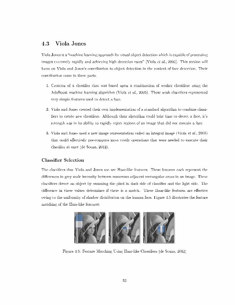
Classi�er Selection
The classi�ers that Viola and Jones use are Haar-like features. These features each represent the
di�erences in grey scale intensity between numerous adjacent rectangular areas in an image. These
classi�ers detect an object by summing the pixel in dark side of classi�er and the light side. The
di�erence in these values determines if there is a match. These Haar-like features are e�ective
owing to the uniformity of shadow distribution on the human face. Figure 4.5 illustrates the feature
matching of the Haar-like features:
Figure 4.5: Feature Matching Using Haar-like Classi�ers (de Souza, 2012)
32
Classi�er Matching
The algorithm to search for a feature match in an image starts by creating a search window on the
image. This section on the image is then searched exhaustively for classi�er matches. On completion
of the search, the search window is adjusted to a di�erent part of the image and repeats the search
process. The search window will have traversed the entire image by the time scanning is complete.
Classi�er matching e�ciently discards search windows that have unpromising results. In search
windows that weakly match a classi�er, more time is spent trying to check that other classi�ers
will not match. When the algorithm eventually cannot reject a search window it concludes that it
contains a face.
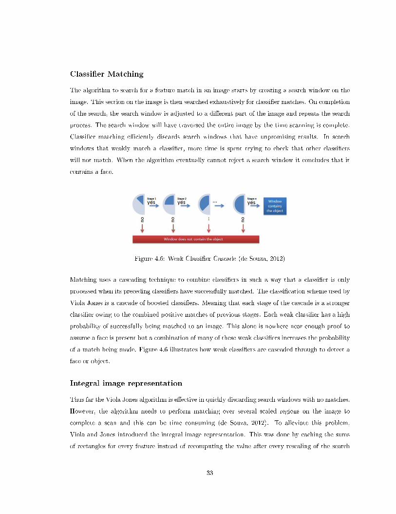
Figure 4.6: Weak Classi�er Cascade (de Souza, 2012)
Matching uses a cascading technique to combine classi�ers in such a way that a classi�er is only
processed when its preceding classi�ers have successfully matched. The classi�cation scheme used by
Viola Jones is a cascade of boosted classi�ers. Meaning that each stage of the cascade is a stronger
classi�er owing to the combined positive matches of previous stages. Each weak classi�er has a high
probability of successfully being matched to an image. This alone is nowhere near enough proof to
assume a face is present but a combination of many of these weak classi�ers increases the probability
of a match being made. Figure 4.6 illustrates how weak classi�ers are cascaded through to detect a
face or object.
Integral image representation
Thus far the Viola Jones algorithm is e�ective in quickly discarding search windows with no matches.
However, the algorithm needs to perform matching over several scaled regions on the image to
complete a scan and this can be time consuming (de Souza, 2012). To alleviate this problem,
Viola and Jones introduced the integral image representation. This was done by caching the sums
of rectangles for every feature instead of recomputing the value after every rescaling of the search
33
window. This was done by creating a summed area table for the frame being processed by computing
all possible rectangular areas in the image. This saves time as it can be computed in a single pass
over the image using the recurrence formula shown in Figure 4.7. Looking at the integral image
representation in Figure 4.7 one can see that the top left value is the same value as original image.
The values adjacent to the top left value of the integral image are then calculated as the sum of
the original images values at this point and any previously calculated adjacent values. The value
13 in the integral image is the sum of its adjacent values 7 and 6. These calculations are performed
throughout the image.
Figure 4.7: Recurrence Formula and Integral Image Example (de Souza, 2012)
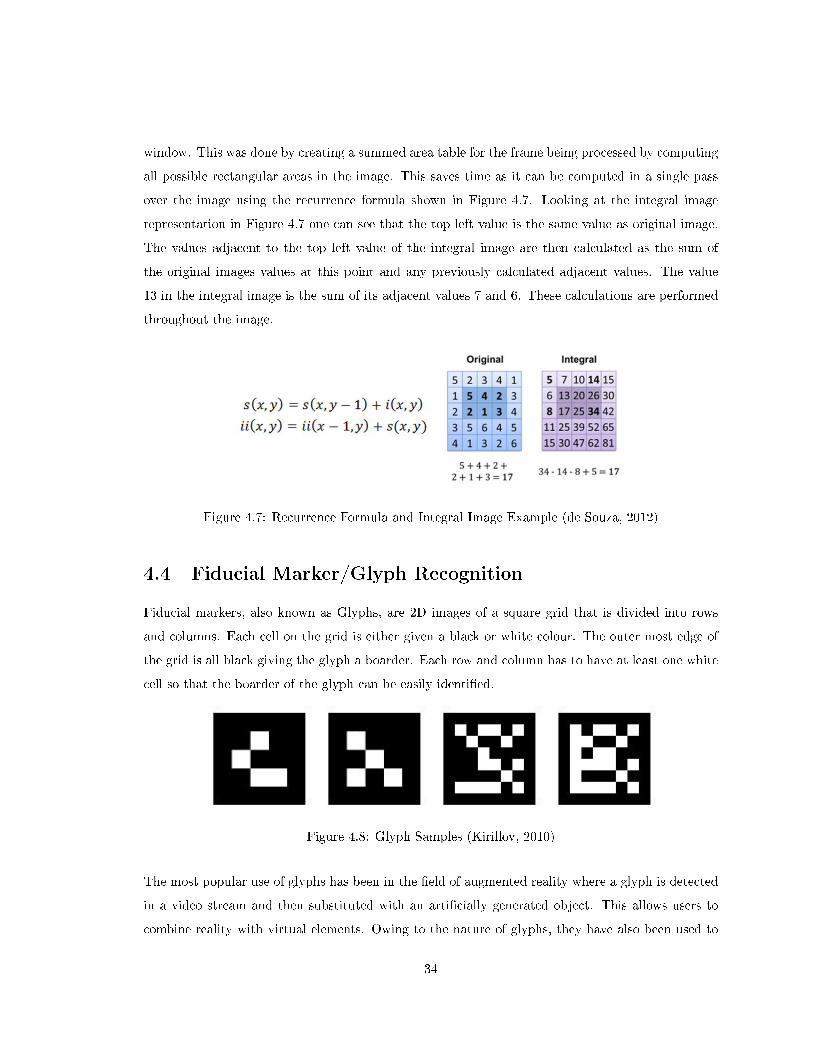
4.4 Fiducial Marker/Glyph Recognition
Fiducial markers, also known as Glyphs, are 2D images of a square grid that is divided into rows
and columns. Each cell on the grid is either given a black or white colour. The outer most edge of
the grid is all black giving the glyph a boarder. Each row and column has to have at least one white
cell so that the boarder of the glyph can be easily identi�ed.
Figure 4.8: Glyph Samples (Kirillov, 2010)
The most popular use of glyphs has been in the �eld of augmented reality where a glyph is detected
in a video stream and then substituted with an arti�cially generated object. This allows users to
combine reality with virtual elements. Owing to the nature of glyphs, they have also been used to
34
provide instructions to robots such as navigation commands as each individual glyph can be easily
told apart.
Finding potential glyphs
Before glyphs can be told apart, the image feed needs to be analysed to search for potential glyphs.
This task involves �nding all quadrilateral areas that bear the attributes of a glyph. Finding the
four corners of the glyph serves as a mechanism to locate glyphs. This can be performed using
various image processing techniques such as grey scaling and thresholding. Grey scaling the image
is the �rst logical step as colour is not needed to recognise glyphs. Grey scaling reduces the size of
an images representation and removes the unnecessary noise of colour from the image. Grey scaling
can be performed in various ways but most methods use percentages of an images red, green and
blue (RGB) pixel values to calculate a single grey scale value for that pixel. An example of this
calculation is as follows:
Gray = 0.299 x Red + 0.587 x Green + 0.114 x Blue
To further isolate the glyphs a custom threshold must be applied to image taking into account the
various lighting conditions of the image. A particularly e�ective thresholding technique for this is
Otsu's thresholding method.
Otsu's Thresholding Method
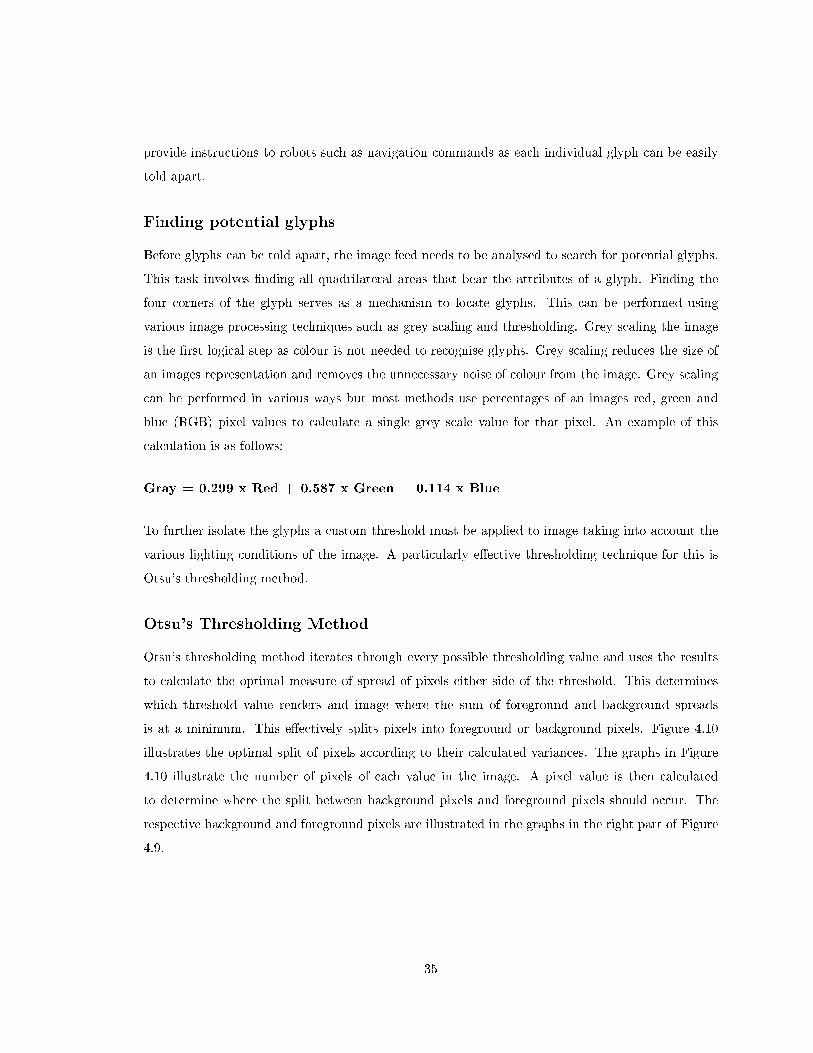
Otsu's thresholding method iterates through every possible thresholding value and uses the results
to calculate the optimal measure of spread of pixels either side of the threshold. This determines
which threshold value renders and image where the sum of foreground and background spreads
is at a minimum. This e�ectively splits pixels into foreground or background pixels. Figure 4.10
illustrates the optimal split of pixels according to their calculated variances. The graphs in Figure
4.10 illustrate the number of pixels of each value in the image. A pixel value is then calculated
to determine where the split between background pixels and foreground pixels should occur. The
respective background and foreground pixels are illustrated in the graphs in the right part of Figure
4.9.
35
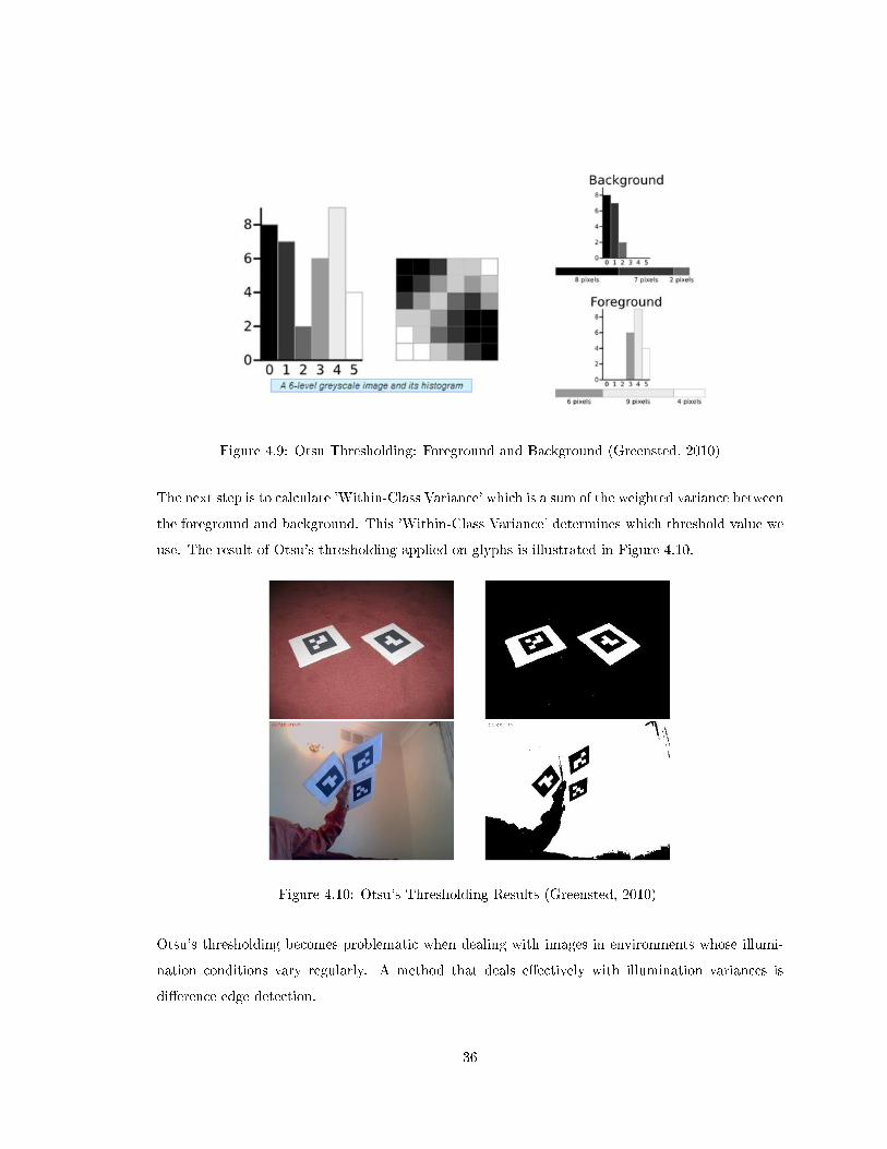
Figure 4.9: Otsu Thresholding: Foreground and Background (Greensted, 2010)
The next step is to calculate 'Within-Class Variance' which is a sum of the weighted variance between
the foreground and background. This 'Within-Class Variance' determines which threshold value we
use. The result of Otsu's thresholding applied on glyphs is illustrated in Figure 4.10.
Figure 4.10: Otsu's Thresholding Results (Greensted, 2010)
Otsu's thresholding becomes problematic when dealing with images in environments whose illumi-
nation conditions vary regularly. A method that deals e�ectively with illumination variances is
di�erence edge detection.
36
Glyph Recognition
Once a glyph has been found it can be extracted from the main image using Quadrilateral Trans-
formation. This transforms any quadrilateral from an image into a rectangular image. Many glyph
images that are detected will be at various angles and depths and so quadrilateral transformation
serves to standardise the image to be input to the glyph recognition algorithm.
Figure 4.11: Glyph Grid Remapping (Kirillov, 2010)
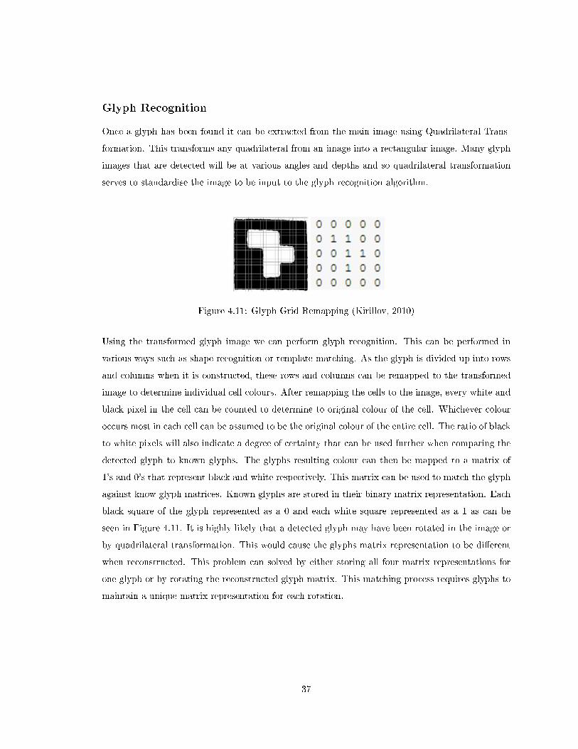
Using the transformed glyph image we can perform glyph recognition. This can be performed in
various ways such as shape recognition or template matching. As the glyph is divided up into rows
and columns when it is constructed, these rows and columns can be remapped to the transformed
image to determine individual cell colours. After remapping the cells to the image, every white and
black pixel in the cell can be counted to determine to original colour of the cell. Whichever colour
occurs most in each cell can be assumed to be the original colour of the entire cell. The ratio of black
to white pixels will also indicate a degree of certainty that can be used further when comparing the
detected glyph to known glyphs. The glyphs resulting colour can then be mapped to a matrix of
1's and 0's that represent black and white respectively. This matrix can be used to match the glyph
against know glyph matrices. Known glyphs are stored in their binary matrix representation. Each
black square of the glyph represented as a 0 and each white square represented as a 1 as can be
seen in Figure 4.11. It is highly likely that a detected glyph may have been rotated in the image or
by quadrilateral transformation. This would cause the glyphs matrix representation to be di�erent
when reconstructed. This problem can solved by either storing all four matrix representations for
one glyph or by rotating the reconstructed glyph matrix. This matching process requires glyphs to
maintain a unique matrix representation for each rotation.
37
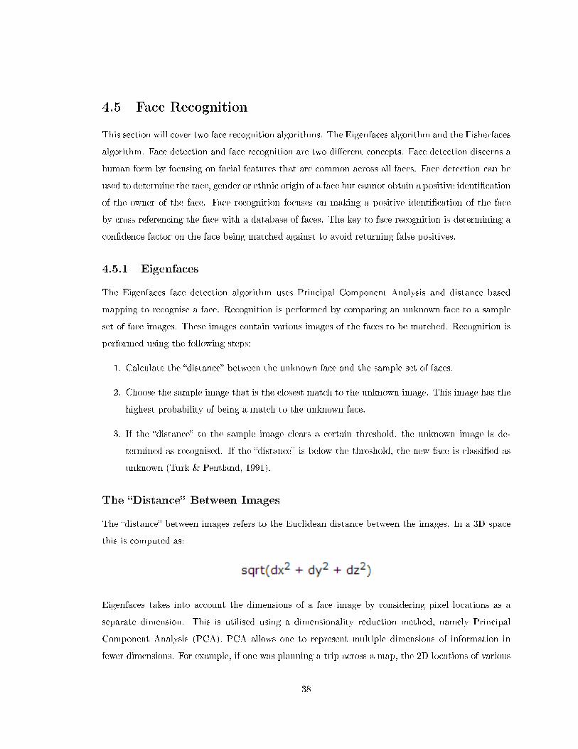
4.5 Face Recognition
This section will cover two face recognition algorithms. The Eigenfaces algorithm and the Fisherfaces
algorithm. Face detection and face recognition are two di�erent concepts. Face detection discerns a
human form by focusing on facial features that are common across all faces. Face detection can be
used to determine the race, gender or ethnic origin of a face but cannot obtain a positive identi�cation
of the owner of the face. Face recognition focuses on making a positive identi�cation of the face
by cross referencing the face with a database of faces. The key to face recognition is determining a
con�dence factor on the face being matched against to avoid returning false positives.
4.5.1 Eigenfaces
The Eigenfaces face detection algorithm uses Principal Component Analysis and distance based
mapping to recognise a face. Recognition is performed by comparing an unknown face to a sample
set of face images. These images contain various images of the faces to be matched. Recognition is
performed using the following steps:
1. Calculate the �distance� between the unknown face and the sample set of faces.
2. Choose the sample image that is the closest match to the unknown image. This image has the
highest probability of being a match to the unknown face.
3. If the �distance� to the sample image clears a certain threshold, the unknown image is de-
termined as recognised. If the �distance� is below the threshold, the new face is classi�ed as
unknown (Turk & Pentland, 1991).
The �Distance� Between Images
The �distance� between images refers to the Euclidean distance between the images. In a 3D space
this is computed as:
Eigenfaces takes into account the dimensions of a face image by considering pixel locations as a
separate dimension. This is utilised using a dimensionality reduction method, namely Principal
Component Analysis (PCA). PCA allows one to represent multiple dimensions of information in
fewer dimensions. For example, if one was planning a trip across a map, the 2D locations of various
38
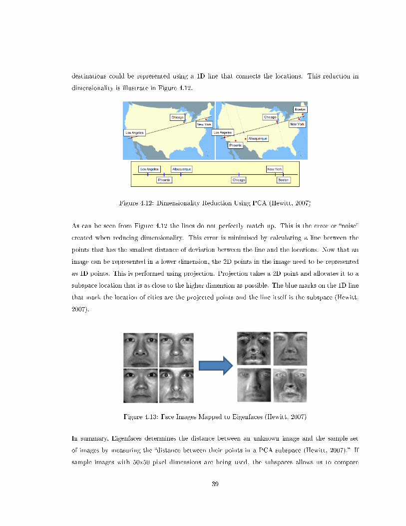
destinations could be represented using a 1D line that connects the locations. This reduction in
dimensionality is illustrate in Figure 4.12.
Figure 4.12: Dimensionality Reduction Using PCA (Hewitt, 2007)
As can be seen from Figure 4.12 the lines do not perfectly match up. This is the error or �noise�
created when reducing dimensionality. This error is minimised by calculating a line between the
points that has the smallest distance of deviation between the line and the locations. Now that an
image can be represented in a lower dimension, the 2D points in the image need to be represented
as 1D points. This is performed using projection. Projection takes a 2D point and allocates it to a
subspace location that is as close to the higher dimension as possible. The blue marks on the 1D line
that mark the location of cities are the projected points and the line itself is the subspace (Hewitt,
2007).
Figure 4.13: Face Images Mapped to Eigenfaces (Hewitt, 2007)
In summary, Eigenfaces determines the distance between an unknown image and the sample set
of images by measuring the �distance between their points in a PCA subspace (Hewitt, 2007).� If
sample images with 50x50 pixel dimensions are being used, the subspaces allows us to compare
39
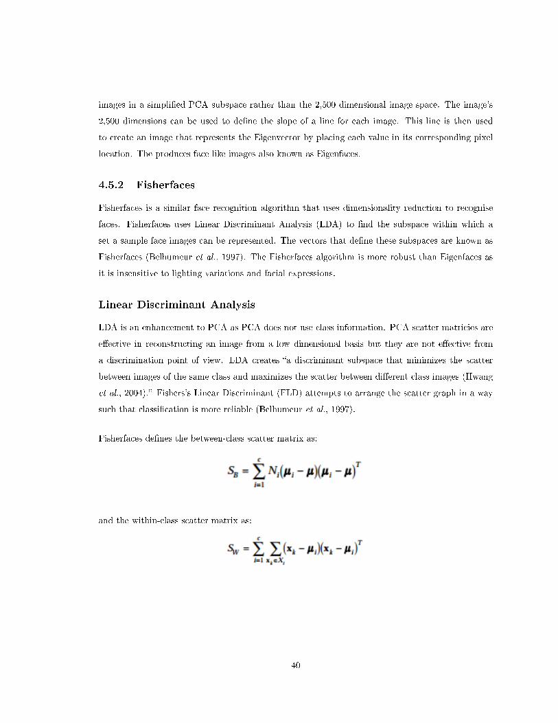
images in a simpli�ed PCA subspace rather than the 2,500 dimensional image space. The image's
2,500 dimensions can be used to de�ne the slope of a line for each image. This line is then used
to create an image that represents the Eigenvector by placing each value in its corresponding pixel
location. The produces face like images also known as Eigenfaces.
4.5.2 Fisherfaces
Fisherfaces is a similar face recognition algorithm that uses dimensionality reduction to recognise
faces. Fisherfaces uses Linear Discriminant Analysis (LDA) to �nd the subspace within which a
set a sample face images can be represented. The vectors that de�ne these subspaces are known as
Fisherfaces (Belhumeur et al., 1997). The Fisherfaces algorithm is more robust than Eigenfaces as
it is insensitive to lighting variations and facial expressions.
Linear Discriminant Analysis
LDA is an enhancement to PCA as PCA does not use class information. PCA scatter matricies are
e�ective in reconstructing an image from a low dimensional basis but they are not e�ective from
a discrimination point of view. LDA creates �a discriminant subspace that minimizes the scatter
between images of the same class and maximizes the scatter between di�erent class images (Hwang
et al., 2004).� Fishers's Linear Discriminant (FLD) attempts to arrange the scatter graph in a way
such that classi�cation is more reliable (Belhumeur et al., 1997).
Fisherfaces de�nes the between-class scatter matrix as:
and the within-class scatter matrix as:
40
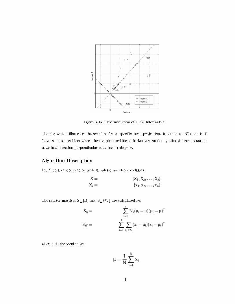
Figure 4.14: Discrimination of Class Information
The Figure 4.14 illustrates the bene�ts of class speci�c linear projection. It compares PCA and FLD
for a two-class problem where the samples used for each class are randomly altered form its normal
state in a direction perpendicular to a linear subspace.
Algorithm Description
Let X be a random vector with samples drawn from c classes:
The scatter matrices S_{B} and S_{W} are calculated as:
where m is the total mean:
41
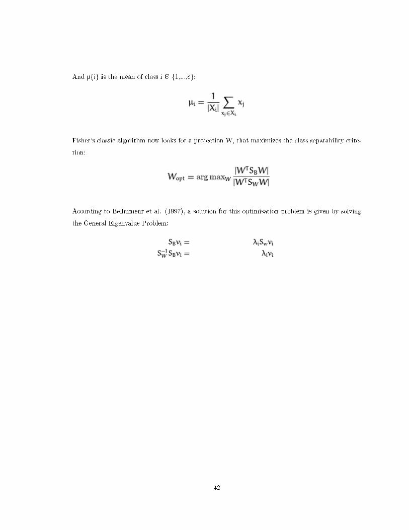
And m{i} is the mean of class i � {1,...,c}:
Fisher's classic algorithm now looks for a projection W, that maximizes the class separability crite-
rion:
According to Belhumeur et al. (1997), a solution for this optimisation problem is given by solving
the General Eigenvalue Problem:
42
Chapter 5
Implementation
5.1 Introduction
The following chapter deals with the implementation of various tracking algorithms. The implemen-
tation was performed across a range of mediums including C++, python and EZ-B. Implementation
began with the goal of determining whether a quadrotor is a feasible medium to execute detection,
recognition and tracking. To test this, various methods of detection and tracking were implemented.
The following sections will cover the implementation of CamShift tacking, Haar-Cascade tracking,
�ducial marker/glyph recognition and the tracking implementation. Many of the algorithms make
use of OpenCV. The version that has been used in these implementations is version 2.4.6.
5.2 Connecting to the AR Drone
To connect to the AR Drone, the Parrot SDK 2.0 was used. The drone uses a Wi-Fi connection
to connect to a client program. The AR Drone can be controlled by any device that can support a
Wi-Fi connection. The connection process is as follows:
1. When the drone is powered up it creates a Wi-Fi network with the default ESSID of the format
ardrone_xxx where xxx is a random sequence of numbers. The drone then allocates itself an
odd IP address on the network (most commonly 192.168.1.1).
2. The user then connects a client device to the networked. This can be a smart phone or PC.
3. As the drone is acting as the server, the client device requests an IP address from the drones
DHCP server.
43
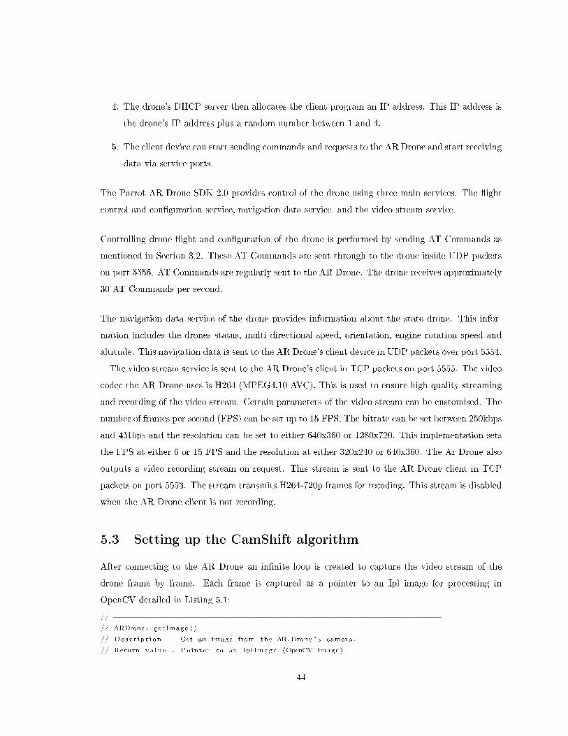
4. The drone's DHCP server then allocates the client program an IP address. This IP address is
the drone's IP address plus a random number between 1 and 4.
5. The client device can start sending commands and requests to the AR Drone and start receiving
data via service ports.
The Parrot AR Drone SDK 2.0 provides control of the drone using three main services. The �ight
control and con�guration service, navigation data service, and the video stream service.
Controlling drone �ight and con�guration of the drone is performed by sending AT Commands as
mentioned in Section 3.2. These AT Commands are sent through to the drone inside UDP packets
on port 5556. AT Commands are regularly sent to the AR Drone. The drone receives approximately
30 AT Commands per second.
The navigation data service of the drone provides information about the state drone. This infor-
mation includes the drones status, multi directional speed, orientation, engine rotation speed and
altitude. This navigation data is sent to the AR Drone's client device in UDP packets over port 5554.
The video stream service is sent to the AR Drone's client in TCP packets on port 5555. The video
codec the AR Drone uses is H264 (MPEG4.10 AVC). This is used to ensure high quality streaming
and recording of the video stream. Certain parameters of the video stream can be customised. The
number of frames per second (FPS) can be set up to 15 FPS. The bitrate can be set between 250kbps
and 4Mbps and the resolution can be set to either 640x360 or 1280x720. This implementation sets
the FPS at either 6 or 15 FPS and the resolution at either 320x240 or 640x360. The Ar Drone also
outputs a video recording stream on request. This stream is sent to the AR Drone client in TCP
packets on port 5553. The stream transmits H264-720p frames for recoding. This stream is disabled
when the AR Drone client is not recording.
5.3 Setting up the CamShift algorithm
After connecting to the AR Drone an in�nite loop is created to capture the video stream of the
drone frame by frame. Each frame is captured as a pointer to an Ipl image for processing in
OpenCV detailed in Listing 5.1:
// −−−−−−−−−−−−−−−−−−−−−−−−−−−−−−−−−−−−−−−−−−−−−−−−−−−−−−−−−−−−−−−−−−−−−−−−−−
// ARDrone : : getImage ( )
// Desc r ip t i on : Get an image from the AR. Drone ' s camera .
// Return value : Po inter to an IplImage (OpenCV image )
44
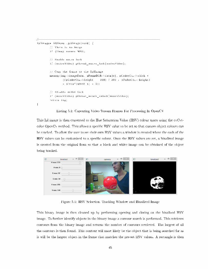
//−−−−−−−−−−−−−−−−−−−−−−−−−−−−−−−−−−−−−−−−−−−−−−−−−−−−−−−−−−−−−−−−−−−−−−−−−−
IplImage * ARDrone : : getImage ( void ) {
// There i s no image
i f ( ! img ) re turn NULL;
// Enable mutex lock
i f (mutexVideo ) pthread_mutex_lock (mutexVideo ) ;
// Copy the frame to the IplImage
memcpy( img−>imageData , pFrameBGR−>data [ 0 ] , pCodecCtx−>width *
( ( pCodecCtx−>height == 368) ? 360 : pCodecCtx−>height )
* s i z e o f ( uint8_t ) * 3 ) ;
// Disab le mutex lock
i f (mutexVideo ) pthread_mutex_unlock (mutexVideo ) ;
r e turn img ;
}
Listing 5.1: Capturing Video Stream Frames For Processing In OpenCV
This Ipl image is then converted to the Hue Saturation Value (HSV) colour space using the cvCvt-
color OpenCv method. This allows a speci�c HSV value to be set so that custom object colours can
be tracked. To allow the user to set their own HSV values a window is created where the each of the
HSV values can be customised to a speci�c colour. Once the HSV values are set, a binalized image
is created from the original from so that a black and white image can be obtained of the object
being tracked.
Figure 5.1: HSV Selection, Tracking Window and Binalized Image
This binary image is then cleaned up by performing opening and closing on the binalized HSV
image. To further identify objects in the binary image a contour search is performed. This retrieves
contours from the binary image and returns the number of contours retrieved. The largest of all
the contours is then found. This contour will most likely be the object that is being searched for as
it will be the largest object in the frame that matches the pre-set HSV values. A rectangle is then
45
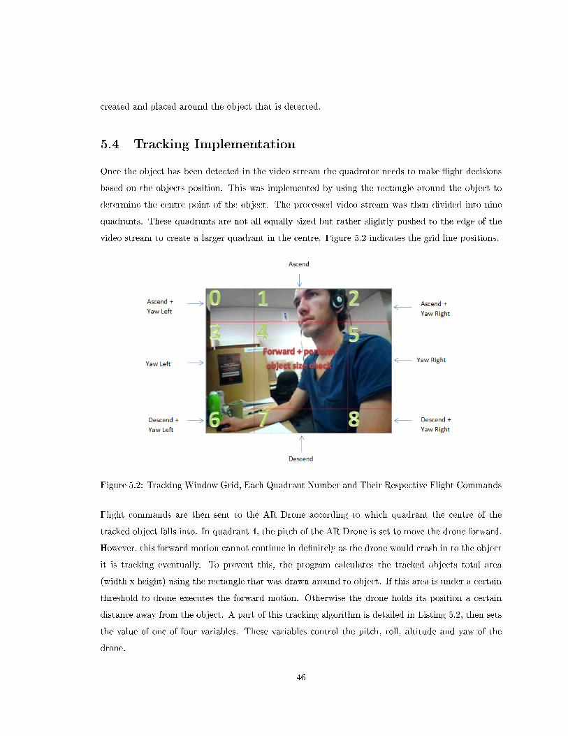
created and placed around the object that is detected.
5.4 Tracking Implementation
Once the object has been detected in the video stream the quadrotor needs to make �ight decisions
based on the objects position. This was implemented by using the rectangle around the object to
determine the centre point of the object. The processed video stream was then divided into nine
quadrants. These quadrants are not all equally sized but rather slightly pushed to the edge of the
video stream to create a larger quadrant in the centre. Figure 5.2 indicates the grid line positions.
Figure 5.2: Tracking Window Grid, Each Quadrant Number and Their Respective Flight Commands
Flight commands are then sent to the AR Drone according to which quadrant the centre of the
tracked object falls into. In quadrant 4, the pitch of the AR Drone is set to move the drone forward.
However, this forward motion cannot continue in de�nitely as the drone would crash in to the object
it is tracking eventually. To prevent this, the program calculates the tracked objects total area
(width x height) using the rectangle that was drawn around to object. If this area is under a certain
threshold to drone executes the forward motion. Otherwise the drone holds its position a certain
distance away from the object. A part of this tracking algorithm is detailed in Listing 5.2, then sets
the value of one of four variables. These variables control the pitch, roll, altitude and yaw of the
drone.
46
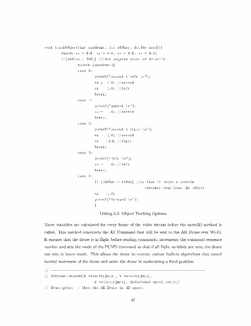
void trackObject ( i n t quadrant , i n t obSize , double a r r [ ] ) {
double vx = 0 . 0 , vy = 0 . 0 , vz = 0 . 0 , vr = 0 . 0 ;
i f ( obSize > 200){ // t h i s negates e r r o r o f d e t e c t i on
switch ( quadrant ){
case 0 :
p r i n t f (" ascend + l e f t \n " ) ;
vz = 1 . 0 ; // ascend
vr = 1 . 0 ; // l e f t
break ;
case 1 :
p r i n t f (" ascend \n " ) ;
vz = 1 . 0 ; // ascend
break ;
case 2 :
p r i n t f (" ascend + r i gh t \n " ) ;
vz = 1 . 0 ; // ascend
vr = −1.0; // r i g h t
break ;
case 3 :
p r i n t f (" l e f t \n " ) ;
vr = 1 . 0 ; // l e f t
break ;
case 4 :
i f ( obSize < 1500){ // so that i t s tay s a c e r t a i n
d i s t anc e away from the ob j e c t
vx = 1 . 0 ;
p r i n t f (" forward \n " ) ;
}
Listing 5.2: Object Tracking Options
These variables are calculated for every frame of the video stream before the move3D method is
called. This method constructs the AT Command that will be sent to the AR Drone over Wi-Fi.
It ensures that the drone is in �ight before sending commands, increments the command sequence
number and sets the mode of the PCMD command so that if all �ight variables are zero, the drone
can rest in hover mode. This allows the drone to execute various built-in algorithms that cancel
inertial movement of the drone and assist the drone in maintaining a �xed position.
// −−−−−−−−−−−−−−−−−−−−−−−−−−−−−−−−−−−−−−−−−−−−−−−−−−−−−−−−−−−−−−−−−−−−−−−−−−
// ARDrone : : move3D(X v e l o c i t y [m/ s ] , Y v e l o c i t y [m/ s ] ,
Z v e l o c i t y [m/ s ] , Rotat iona l speed [ rad/ s ] )
// Desc r ip t i on : Move the AR. Drone in 3D space .
47

// Return value : NONE
// −−−−−−−−−−−−−−−−−−−−−−−−−−−−−−−−−−−−−−−−−−−−−−−−−−−−−−−−−−−−−−−−−−−−−−−−−−
void ARDrone : : move3D( double vx , double vy , double vz , double vr ) {
// AR. Drone i s f l y i n g
i f ( ! onGround ( ) ) {
// Command v e l o c i t i e s
f l o a t v [ 4 ] = {−vy *0 . 2 , −vx *1 . 0 , vz *0 . 1 , −vr *0 . 5 } ;
i n t mode = ( fabs ( v [ 0 ] ) > 0 .0 | | f abs ( v [ 1 ] ) > 0 .0 | |
f abs ( v [ 2 ] ) > 0 .0 | | f abs ( v [ 3 ] ) > 0 . 0 ) ;
// L imitat ion (−1.0 to +1.0)
f o r ( i n t i = 0 ; i < 4 ; i++) {
i f ( f abs ( v [ i ] ) > 1 . 0 ) v [ i ] /= fabs (v [ i ] ) ;
}
// Send a command
i f (mutexCommand) pthread_mutex_lock (mutexCommand ) ;
sockCommand . sendf ("AT*PCMD=%d,%d,%d,%d,%d,%d\ r " ,
++seq , mode , *( i n t *)(&v [ 0 ] ) , *( i n t *)(&v [ 1 ] ) ,
*( i n t *)(&v [ 2 ] ) , *( i n t *)(&v [ 3 ] ) ) ;
i f (mutexCommand) pthread_mutex_unlock (mutexCommand ) ;
}
}
Listing 5.3: AR Drone move3D Method
This algorithm created erratic �ight in the AR Drone as it received numerous tacking commands
every 30ms. This was overcome by sleeping the main method for 200ms to accommodate for motion
delay. This helps to prevent the drone from executing a descend command 30ms after it started an
ascend command. This also stops the occurance of �bounce� during �ight. This could be caused by
the drone executing, for example, an ascend command but instead of the object being centred within
quadrant four the movement passes over quadrant four and straight into quadrant seven where a
descend command will be sent immediately.
5.5 Setting up the various human feature tracking using Haar
Cascades
In this section, the use of various Haar Cascades for tracking purposes is implemented. Each Haar
Cascade uses OpenCV to track a human feature based on its speci�c classi�er cascade. The cascades
are constructed within XML �les which contain various pieces of information about each classi�er.
48
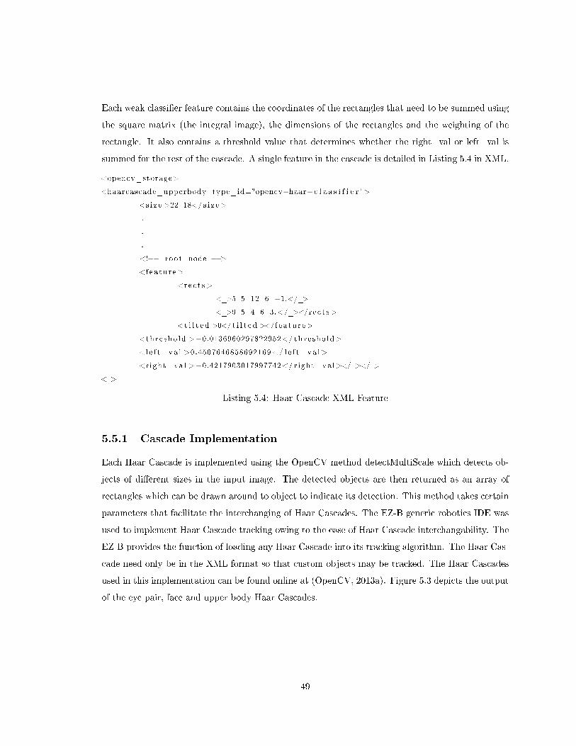
Each weak classi�er feature contains the coordinates of the rectangles that need to be summed using
the square matrix (the integral image), the dimensions of the rectangles and the weighting of the
rectangle. It also contains a threshold value that determines whether the right_val or left_val is
summed for the rest of the cascade. A single feature in the cascade is detailed in Listing 5.4 in XML.
<opencv_storage>
<haarcascade_upperbody type_id="opencv−haar−c l a s s i f i e r ">
<s i z e >22 18</ s i z e >
.
.
.
<!−− root node −−>
<feature>
<rec t s >
<_>5 5 12 6 −1.</_>
<_>9 5 4 6 3.</_></rec t s >
<t i l t e d >0</t i l t e d ></fea ture>
<thresho ld >−0.0136960297822952</ thresho ld>
<le f t_va l >0.4507646858692169</ le f t_va l>
<right_val >−0.4217903017997742</ right_val></_></_>
<_>
Listing 5.4: Haar Cascade XML Feature
5.5.1 Cascade Implementation
Each Haar Cascade is implemented using the OpenCV method detectMultiScale which detects ob-
jects of di�erent sizes in the input image. The detected objects are then returned as an array of
rectangles which can be drawn around to object to indicate its detection. This method takes certain
parameters that facilitate the interchanging of Haar Cascades. The EZ-B generic robotics IDE was
used to implement Haar Cascade tracking owing to the ease of Haar Cascade interchangability. The
EZ-B provides the function of loading any Haar Cascade into its tracking algorithm. The Haar Cas-
cade need only be in the XML format so that custom objects may be tracked. The Haar Cascades
used in this implementation can be found online at (OpenCV, 2013a). Figure 5.3 depicts the output
of the eye pair, face and upper body Haar Cascades.
49
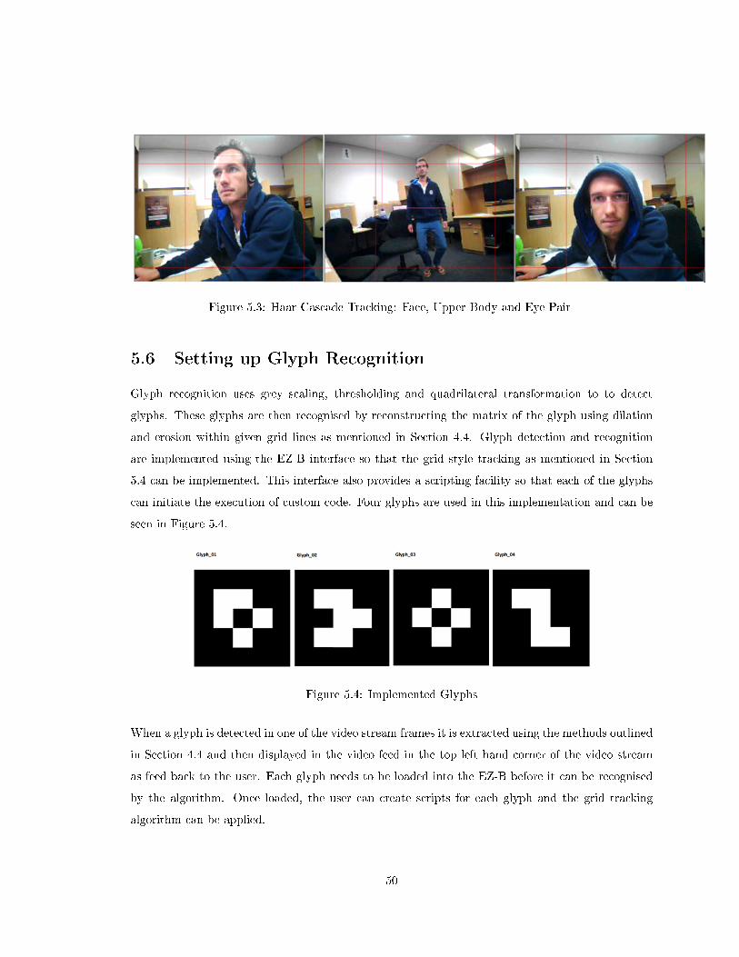
Figure 5.3: Haar Cascade Tracking: Face, Upper Body and Eye Pair
5.6 Setting up Glyph Recognition
Glyph recognition uses grey scaling, thresholding and quadrilateral transformation to to detect
glyphs. These glyphs are then recognised by reconstructing the matrix of the glyph using dilation
and erosion within given grid lines as mentioned in Section 4.4. Glyph detection and recognition
are implemented using the EZ-B interface so that the grid style tracking as mentioned in Section
5.4 can be implemented. This interface also provides a scripting facility so that each of the glyphs
can initiate the execution of custom code. Four glyphs are used in this implementation and can be
seen in Figure 5.4.
Figure 5.4: Implemented Glyphs
When a glyph is detected in one of the video stream frames it is extracted using the methods outlined
in Section 4.4 and then displayed in the video feed in the top left hand corner of the video stream
as feed back to the user. Each glyph needs to be loaded into the EZ-B before it can be recognised
by the algorithm. Once loaded, the user can create scripts for each glyph and the grid tracking
algorithm can be applied.
50

Figure 5.5: Glyph Detection and Recognition
5.7 Face recognition using Fisherfaces
The �rst step in implementing a face recognition program is to acquire a database of face images.
This implementation makes use of the AT&T Facedatabase (Cambridge, 2002) with the addition
of some new faces. The AT&T database contains face images of 40 di�erent people. Each person
has ten di�erent images of their faces in the database. Each picture was taken at di�erent times
and is subject to di�erent lighting conditions and facial expressions. The facial expressions can be
of someone with their mouth open, closed or smiling, . Facial details in the photos also changes
as some pictures are of the subject wearing glasses where others are not. All images in the AT&T
Facedatabase have been taken against a homogeneous, dark background with the subject in a upright,
front facing position. In addition to the AT&T Facedatabase images, three additional subjects were
added to the photo collection.
5.7.1 Creating a Custom Image Database
The images added to the existing AT&T needed to be edited. This editing was done by cropping the
face according to the position of the subjects eyes. This editing allows the Fisherfaces algorithm to
focus on extracting features from the face that are robust to illumination, background interference
and changes in the subject's hair. A python script was use to perform this editing. The cropping
51
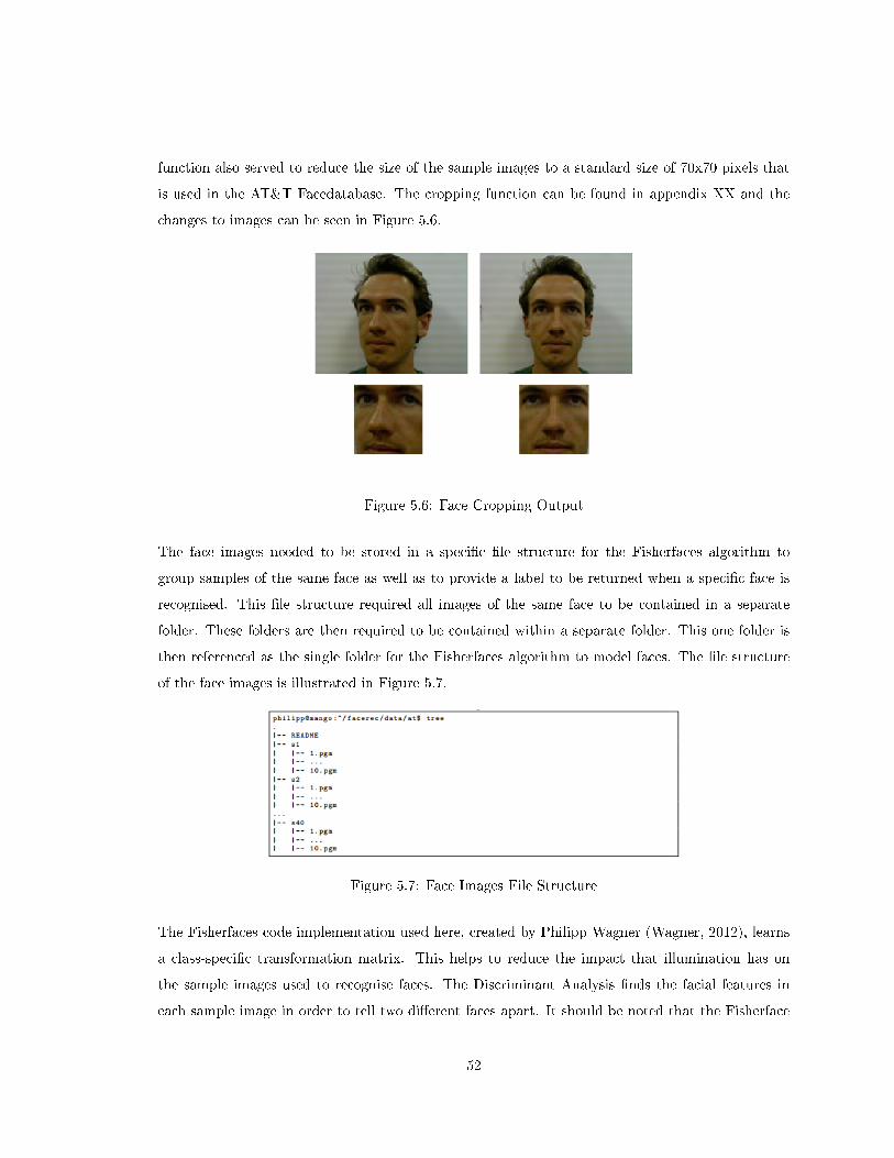
function also served to reduce the size of the sample images to a standard size of 70x70 pixels that
is used in the AT&T Facedatabase. The cropping function can be found in appendix XX and the
changes to images can be seen in Figure 5.6.
Figure 5.6: Face Cropping Output
The face images needed to be stored in a speci�c �le structure for the Fisherfaces algorithm to
group samples of the same face as well as to provide a label to be returned when a speci�c face is
recognised. This �le structure required all images of the same face to be contained in a separate
folder. These folders are then required to be contained within a separate folder. This one folder is
then referenced as the single folder for the Fisherfaces algorithm to model faces. The �le structure
of the face images is illustrated in Figure 5.7.
Figure 5.7: Face Images File Structure
The Fisherfaces code implementation used here, created by Philipp Wagner (Wagner, 2012), learns
a class-speci�c transformation matrix. This helps to reduce the impact that illumination has on
the sample images used to recognise faces. The Discriminant Analysis �nds the facial features in
each sample image in order to tell two di�erent faces apart. It should be noted that the Fisherface
52

algorithm's performance strongly relies on the input data. That is to say, in practice, the Fisherfaces
algorithm will not perform well if the sample pictures used to train Fisherfaces are taken in a well
illuminated environment and the faces that are trying to be recognised are input from a badly
illuminated environment. This occurs as the features that are predominant in an image di�er when
in environments with vastly di�erent lighting conditions.
53
Chapter 6
Testing and Analysis
This chapter details the various tests performed with the AR Drone to assess the capabilities of each
algorithm with respect to detection, tracking and recognition. This chapter is split into four parts:
detection testing, detection at angles, recognition testing and tracking testing.
6.1 Detection Testing
To assess the e�ectiveness of each algorithm with respect to its detection ability, a standard test was
devised. Each algorithm needed to track its respective face, object or marker, hence forth known
as the subject. The subject was placed a speci�c distance away from the camera and executed a
standard set of movements. Each algorithm's detection ability was then assessed according to the
number of frames the subject was detected in, the number of frames in which false detections (false
positives) occured, the rate of false positives and the rate of true positives. The following sections
will report on the performance of each algorithm and outline the speci�cs of each test.
6.1.1 Viola Jones Detection Results
The Viola Jones face detection algorithm uses a cascade of weak classi�ers (Haar-like features) to
identify a face according to predominant human facial features. The goal of this algorithm is to
detect a human face in a live video stream. This test has been formulated to test the e�ectiveness
of the Viola Jones face detection algorithm. The following tests were performed using the EZ-B
robotics API. The subject the test is performed on starts o� directly facing the camera in a seated
position. This position is held for �ve seconds. The subject then leans to the left and holds this
54
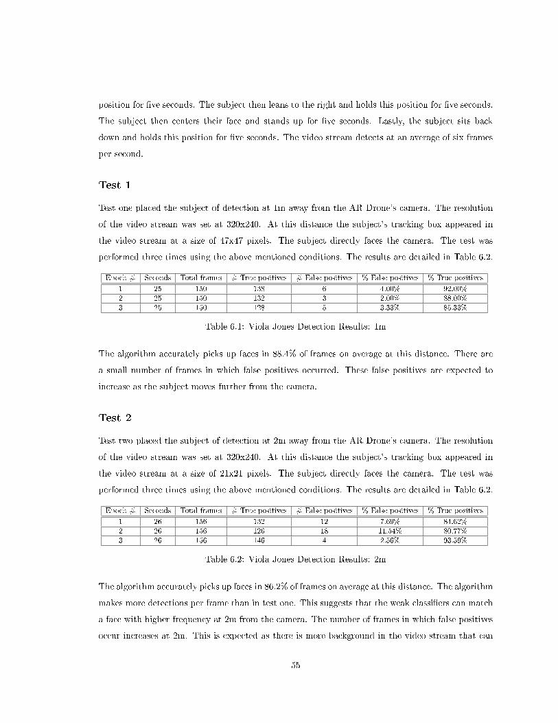
position for �ve seconds. The subject then leans to the right and holds this position for �ve seconds.
The subject then centers their face and stands up for �ve seconds. Lastly, the subject sits back
down and holds this position for �ve seconds. The video stream detects at an average of six frames
per second.
Test 1
Test one placed the subject of detection at 1m away from the AR Drone's camera. The resolution
of the video stream was set at 320x240. At this distance the subject's tracking box appeared in
the video stream at a size of 47x47 pixels. The subject directly faces the camera. The test was
performed three times using the above mentioned conditions. The results are detailed in Table 6.2.
Epoch # Seconds Total frames # True positives # False positives % False positives % True positives
1 25 150 138 6 4.00% 92.00%2 25 150 132 3 2.00% 88.00%3 25 150 128 5 3.33% 85.33%
Table 6.1: Viola Jones Detection Results: 1m
The algorithm accurately picks up faces in 88.4% of frames on average at this distance. There are
a small number of frames in which false positives occurred. These false positives are expected to
increase as the subject moves further from the camera.
Test 2
Test two placed the subject of detection at 2m away from the AR Drone's camera. The resolution
of the video stream was set at 320x240. At this distance the subject's tracking box appeared in
the video stream at a size of 21x21 pixels. The subject directly faces the camera. The test was
performed three times using the above mentioned conditions. The results are detailed in Table 6.2.
Epoch # Seconds Total frames # True positives # False positives % False positives % True positives
1 26 156 132 12 7.69% 84.62%2 26 156 126 18 11.54% 80.77%3 26 156 146 4 2.56% 93.59%
Table 6.2: Viola Jones Detection Results: 2m
The algorithm accurately picks up faces in 86.2% of frames on average at this distance. The algorithm
makes more detections per frame than in test one. This suggests that the weak classi�ers can match
a face with higher frequency at 2m from the camera. The number of frames in which false positives
occur increases at 2m. This is expected as there is more background in the video stream that can
55
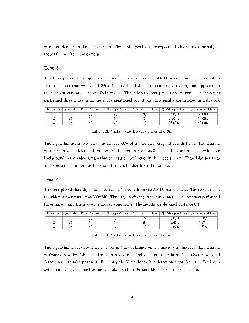
cause interference in the video stream. These false positives are expected to increase as the subject
moves further from the camera.
Test 3
Test three placed the subject of detection at 3m away from the AR Drone's camera. The resolution
of the video stream was set at 320x240. At this distance the subject's tracking box appeared in
the video stream at a size of 15x15 pixels. The subject directly faces the camera. The test was
performed three times using the above mentioned conditions. The results are detailed in Table 6.3.
Epoch # Seconds Total frames # True positives # False positives % False positives % True positives
1 25 150 96 36 24.00% 64.00%2 25 150 84 30 20.00% 56.00%3 25 150 90 42 28.00% 60.00%
Table 6.3: Viola Jones Detection Results: 3m
The algorithm accurately picks up faces in 60% of frames on average at this distance. The number
of frames in which false positives occurred increases again at 3m. This is expected as there is more
background in the video stream that can cause interference in the video stream. These false positives
are expected to increase as the subject moves further from the camera.
Test 4
Test four placed the subject of detection at 5m away from the AR Drone's camera. The resolution of
the video stream was set at 320x240. The subject directly faces the camera. The test was performed
three times using the above mentioned conditions. The results are detailed in Table 6.4.
Epoch # Seconds Total frames # True positives # False positives % False positives % True positives
1 25 150 6 72 48.00% 4.00%2 25 150 10 64 42.67% 6.67%3 25 150 7 70 46.67% 4.67%
Table 6.4: Viola Jones Detection Results: 5m
The algorithm accurately picks up faces in 5.1% of frames on average at this distance. The number
of frames in which false positives occurred dramatically increases again at 5m. Over 89% of all
detections were false positives. Evidently the Viola Jones face detection algorithm is ine�ective in
detecting faces at �ve metres and therefore will not be suitable for use in face tracking.
56
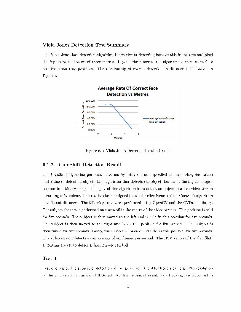
Viola Jones Detection Test Summary
The Viola Jones face detection algorithm is e�ective at detecting faces at this frame rate and pixel
density up to a distance of three metres. Beyond three metres the algorithm detects more false
positives than true positives. The relationship of correct detection to distance is illustrated in
Figure 6.1.
Figure 6.1: Viola Jones Detection Results Graph
6.1.2 CamShift Detection Results
The CamShift algorithm performs detection by using the user speci�ed values of Hue, Saturation
and Value to detect an object. The algorithm that detects the object does so by �nding the largest
contour in a binary image. The goal of this algorithm is to detect an object in a live video stream
according to its colour. This test has been designed to test the e�ectiveness of the CamShift algorithm
at di�erent distances. The following tests were performed using OpenCV and the CVDrone library.
The subject the test is performed on starts o� in the centre of the video stream. This position is held
for �ve seconds. The subject is then moved to the left and is held in this position for �ve seconds.
The subject is then moved to the right and holds this position for �ve seconds. The subject is
then raised for �ve seconds. Lastly, the subject is lowered and held in this position for �ve seconds.
The video stream detects at an average of six frames per second. The HSV values of the CamShift
algorithm are set to detect a distinctively red ball.
Test 1
Test one placed the subject of detection at 1m away from the AR Drone's camera. The resolution
of the video stream was set at 640x480. At this distance the subject's tracking box appeared in
57
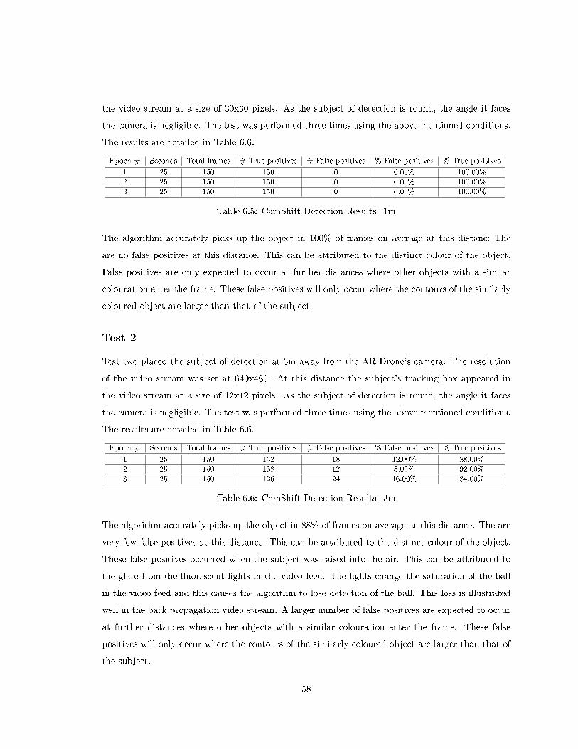
the video stream at a size of 30x30 pixels. As the subject of detection is round, the angle it faces
the camera is negligible. The test was performed three times using the above mentioned conditions.
The results are detailed in Table 6.6.
Epoch # Seconds Total frames # True positives # False positives % False positives % True positives
1 25 150 150 0 0.00% 100.00%2 25 150 150 0 0.00% 100.00%3 25 150 150 0 0.00% 100.00%
Table 6.5: CamShift Detection Results: 1m
The algorithm accurately picks up the object in 100% of frames on average at this distance.The
are no false positives at this distance. This can be attributed to the distinct colour of the object.
False positives are only expected to occur at further distances where other objects with a similar
colouration enter the frame. These false positives will only occur where the contours of the similarly
coloured object are larger than that of the subject.
Test 2
Test two placed the subject of detection at 3m away from the AR Drone's camera. The resolution
of the video stream was set at 640x480. At this distance the subject's tracking box appeared in
the video stream at a size of 12x12 pixels. As the subject of detection is round, the angle it faces
the camera is negligible. The test was performed three times using the above mentioned conditions.
The results are detailed in Table 6.6.
Epoch # Seconds Total frames # True positives # False positives % False positives % True positives
1 25 150 132 18 12.00% 88.00%2 25 150 138 12 8.00% 92.00%3 25 150 126 24 16.00% 84.00%
Table 6.6: CamShift Detection Results: 3m
The algorithm accurately picks up the object in 88% of frames on average at this distance. The are
very few false positives at this distance. This can be attributed to the distinct colour of the object.
These false positives occurred when the subject was raised into the air. This can be attributed to
the glare from the �uorescent lights in the video feed. The lights change the saturation of the ball
in the video feed and this causes the algorithm to lose detection of the ball. This loss is illustrated
well in the back propagation video stream. A larger number of false positives are expected to occur
at further distances where other objects with a similar colouration enter the frame. These false
positives will only occur where the contours of the similarly coloured object are larger than that of
the subject.
58
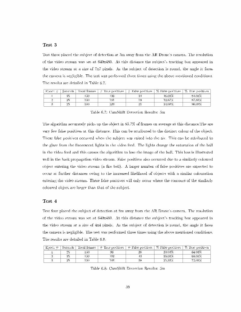
Test 3
Test three placed the subject of detection at 5m away from the AR Drone's camera. The resolution
of the video stream was set at 640x480. At this distance the subject's tracking box appeared in
the video stream at a size of 7x7 pixels. As the subject of detection is round, the angle it faces
the camera is negligible. The test was performed three times using the above mentioned conditions.
The results are detailed in Table 6.7.
Epoch # Seconds Total frames # True positives # False positives % False positives % True positives
1 25 150 126 24 16.00% 84.00%2 25 150 131 19 12.67% 87.33%3 25 150 129 21 14.00% 86.00%
Table 6.7: CamShift Detection Results: 5m
The algorithm accurately picks up the object in 85.7% of frames on average at this distance.The are
very few false positives at this distance. This can be attributed to the distinct colour of the object.
These false positives occurred when the subject was raised into the air. This can be attributed to
the glare from the �uorescent lights in the video feed. The lights change the saturation of the ball
in the video feed and this causes the algorithm to lose the image of the ball. This loss is illustrated
well in the back propagation video stream. False positives also occurred due to a similarly coloured
object entering the video stream (a �re bell). A larger number of false positives are expected to
occur at further distances owing to the increased likelihood of objects with a similar colouration
entering the video stream. These false positives will only occur where the contours of the similarly
coloured object are larger than that of the subject.
Test 4
Test four placed the subject of detection at 8m away from the AR Drone's camera. The resolution
of the video stream was set at 640x480. At this distance the subject's tracking box appeared in
the video stream at a size of 4x4 pixels. As the subject of detection is round, the angle it faces
the camera is negligible. The test was performed three times using the above mentioned conditions.
The results are detailed in Table 6.8.
Epoch # Seconds Total frames # True positives # False positives % False positives % True positives
1 25 150 96 30 20.00% 64.00%2 25 150 102 42 28.00% 68.00%3 25 150 108 38 25.33% 72.00%
Table 6.8: CamShift Detection Results: 5m
59

The algorithm accurately picks up the object in 68% of frames on average at this distance. More
false positives occur at this distance. This can be attributed to more similarly objects entering the
video stream. These false positives occurred again when the subject was raised into the air. This
can be attributed to the glare from the �uorescent lights in the video feed. The lights change the
saturation of the ball in the video feed and this causes the algorithm to lose the image of the ball.
This loss is illustrated well in the back propagation video stream. False positives due to similarly
coloured object entering the video stream (a �re bell, a pair of red shoes). With the subject at a
greater distance from the camera, the contours of the similarly coloured objects can become larger
than that of the subject. This accounts for the majority of false positives that occurred.
CamShift Detection Test Summary
The CamShift algorithm performs e�ectively when tracking a distinctly coloured object at this frame
rate and pixel density up to a distance of �ve metres. The CamShift algorithm produces considerably
less false positives than the Viola Jones face detection algorithm. This remains true even when the
subject of detection is further away from the camera. The use of OpenCV and the CVDrone library
maintained a more stable video feed than the EZ-B as there were fewer instances of the video feed
crashing. There were also fewer instances of video feed transmission delay between the drone and the
client program. According to these results, it is assumed that CamShift will be a robust algorithm to
implement tracking. The relationship of correct detection to distance using the CamShift algorithm
is illustrated in Figure 6.2.
Figure 6.2: CamShift Detection Results Graph
60
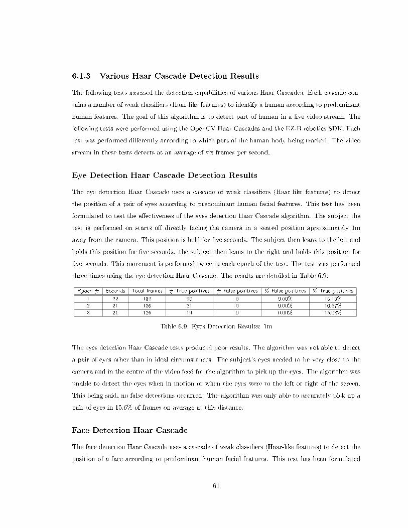
6.1.3 Various Haar Cascade Detection Results
The following tests assessed the detection capabilities of various Haar Cascades. Each cascade con-
tains a number of weak classi�ers (Haar-like features) to identify a human according to predominant
human features. The goal of this algorithm is to detect part of human in a live video stream. The
following tests were performed using the OpenCV Haar Cascades and the EZ-B robotics SDK. Each
test was performed di�erently according to which part of the human body being tracked. The video
stream in these tests detects at an average of six frames per second.
Eye Detection Haar Cascade Detection Results
The eye detection Haar Cascade uses a cascade of weak classi�ers (Haar-like features) to detect
the position of a pair of eyes according to predominant human facial features. This test has been
formulated to test the e�ectiveness of the eyes detection Haar Cascade algorithm. The subject the
test is performed on starts o� directly facing the camera in a seated position approximately 1m
away from the camera. This position is held for �ve seconds. The subject then leans to the left and
holds this position for �ve seconds. the subject then leans to the right and holds this position for
�ve seconds. This movement is performed twice in each epoch of the test. The test was performed
three times using the eye detection Haar Cascade. The results are detailed in Table 6.9.
Epoch # Seconds Total frames # True positives # False positives % False positives % True positives
1 22 132 20 0 0.00% 15.15%2 21 126 21 0 0.00% 16.67%3 21 126 19 0 0.00% 15.08%
Table 6.9: Eyes Detection Results: 1m
The eyes detection Haar Cascade tests produced poor results. The algorithm was not able to detect
a pair of eyes other than in ideal circumstances. The subject's eyes needed to be very close to the
camera and in the centre of the video feed for the algorithm to pick up the eyes. The algorithm was
unable to detect the eyes when in motion or when the eyes were to the left or right of the screen.
This being said, no false detections occurred. The algorithm was only able to accurately pick up a
pair of eyes in 15.6% of frames on average at this distance.
Face Detection Haar Cascade
The face detection Haar Cascade uses a cascade of weak classi�ers (Haar-like features) to detect the
position of a face according to predominant human facial features. This test has been formulated
61
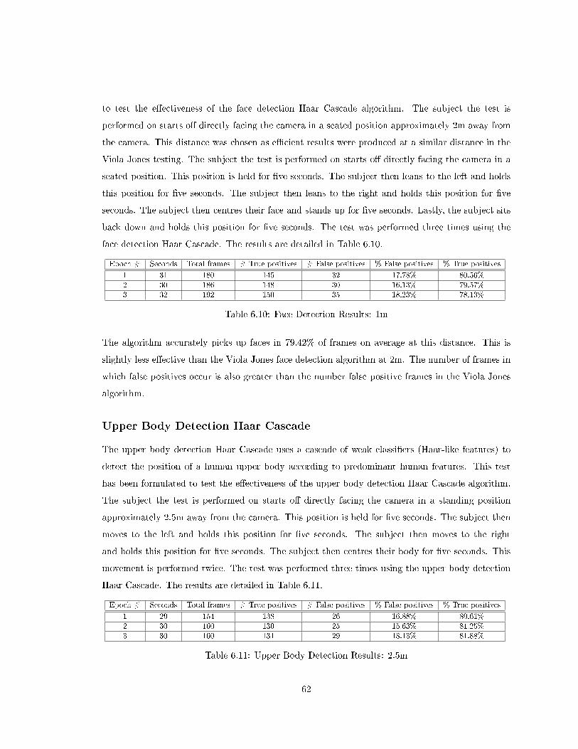
to test the e�ectiveness of the face detection Haar Cascade algorithm. The subject the test is
performed on starts o� directly facing the camera in a seated position approximately 2m away from
the camera. This distance was chosen as e�cient results were produced at a similar distance in the
Viola Jones testing. The subject the test is performed on starts o� directly facing the camera in a
seated position. This position is held for �ve seconds. The subject then leans to the left and holds
this position for �ve seconds. The subject then leans to the right and holds this position for �ve
seconds. The subject then centres their face and stands up for �ve seconds. Lastly, the subject sits
back down and holds this position for �ve seconds. The test was performed three times using the
face detection Haar Cascade. The results are detailed in Table 6.10.
Epoch # Seconds Total frames # True positives # False positives % False positives % True positives
1 31 180 145 32 17.78% 80.56%2 30 186 148 30 16.13% 79.57%3 32 192 150 35 18.23% 78.13%
Table 6.10: Face Detection Results: 1m
The algorithm accurately picks up faces in 79.42% of frames on average at this distance. This is
slightly less e�ective than the Viola Jones face detection algorithm at 2m. The number of frames in
which false positives occur is also greater than the number false positive frames in the Viola Jones
algorithm.
Upper Body Detection Haar Cascade
The upper body detection Haar Cascade uses a cascade of weak classi�ers (Haar-like features) to
detect the position of a human upper body according to predominant human features. This test
has been formulated to test the e�ectiveness of the upper body detection Haar Cascade algorithm.
The subject the test is performed on starts o� directly facing the camera in a standing position
approximately 2.5m away from the camera. This position is held for �ve seconds. The subject then
moves to the left and holds this position for �ve seconds. The subject then moves to the right
and holds this position for �ve seconds. The subject then centres their body for �ve seconds. This
movement is performed twice. The test was performed three times using the upper body detection
Haar Cascade. The results are detailed in Table 6.11.
Epoch # Seconds Total frames # True positives # False positives % False positives % True positives
1 29 154 138 26 16.88% 89.61%2 30 160 130 25 15.63% 81.25%3 30 160 131 29 18.13% 81.88%
Table 6.11: Upper Body Detection Results: 2.5m
62
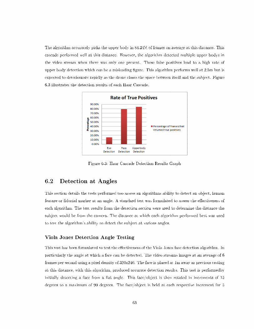
The algorithm accurately picks the upper body in 84.24% of frames on average at this distance. This
cascade performed well at this distance. However, the algorithm detected multiple upper bodys in
the video stream when there was only one present. These false positives lead to a high rate of
upper body detection which can be a misleading �gure. This algorithm performs well at 2.5m but is
expected to deteriourate rapidly as the drone closes the space between itself and the subject. Figure
6.3 illustrates the detection results of each Haar Cascade.
Figure 6.3: Haar Cascade Detection Results Graph
6.2 Detection at Angles
This section details the tests performed too assess an algorithms ability to detect an object, human
feature or �ducial marker at an angle. A standard test was formulated to assess the e�ectiveness of
each algorithm. The test results from the detection section were used to determine the distance the
subject would be from the camera. The distance at which each algorithm performed best was used
to test the algorithm's ability to detect the subject at various angles.
Viola Jones Detection Angle Testing
This test has been formulated to test the e�ectiveness of the Viola Jones face detection algorithm. In
particularly the angle at which a face can be detected. The video streams images at an average of 6
frames per second using a pixel density of 320x240. The face is placed at 1m away as previous testing
at this distance, with this algorithm, produced accurate detection results. This test is performedby
initially detecting a face from a �at angle. This face/object is then rotated in increments of 15
degrees to a maximum of 90 degrees. The face/object is held at each respective increment for 5
63
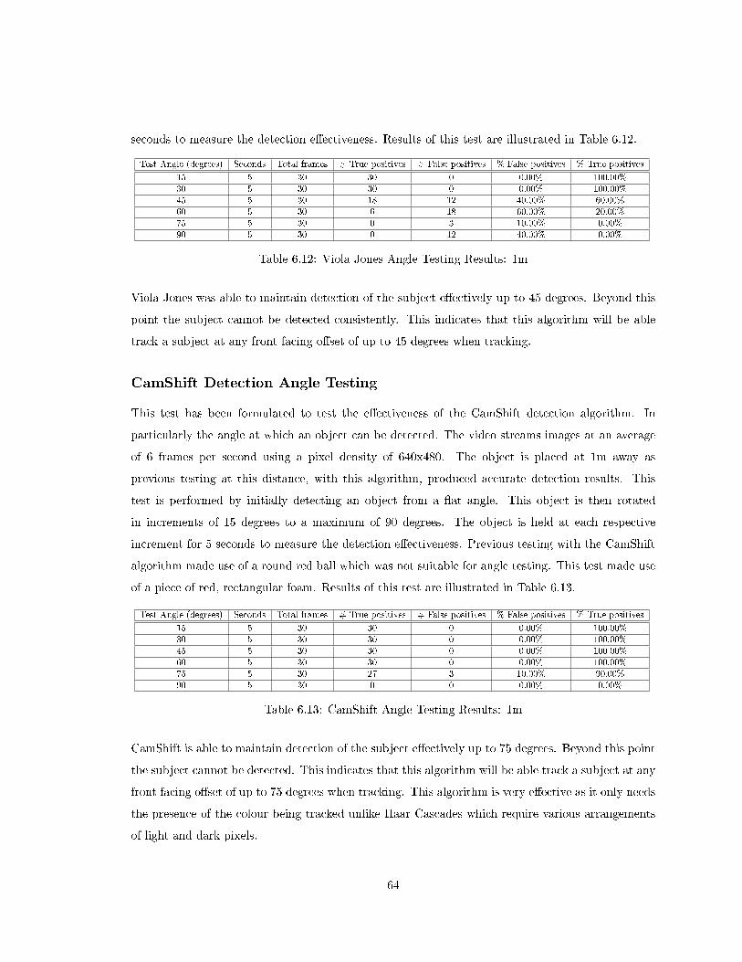
seconds to measure the detection e�ectiveness. Results of this test are illustrated in Table 6.12.
Test Angle (degrees) Seconds Total frames # True positives # False positives % False positives % True positives
15 5 30 30 0 0.00% 100.00%30 5 30 30 0 0.00% 100.00%45 5 30 18 12 40.00% 60.00%60 5 30 6 18 60.00% 20.00%75 5 30 0 3 10.00% 0.00%90 5 30 0 12 40.00% 0.00%
Table 6.12: Viola Jones Angle Testing Results: 1m
Viola Jones was able to maintain detection of the subject e�ectively up to 45 degrees. Beyond this
point the subject cannot be detected consistently. This indicates that this algorithm will be able
track a subject at any front facing o�set of up to 45 degrees when tracking.
CamShift Detection Angle Testing
This test has been formulated to test the e�ectiveness of the CamShift detection algorithm. In
particularly the angle at which an object can be detected. The video streams images at an average
of 6 frames per second using a pixel density of 640x480. The object is placed at 1m away as
previous testing at this distance, with this algorithm, produced accurate detection results. This
test is performed by initially detecting an object from a �at angle. This object is then rotated
in increments of 15 degrees to a maximum of 90 degrees. The object is held at each respective
increment for 5 seconds to measure the detection e�ectiveness. Previous testing with the CamShift
algorithm made use of a round red ball which was not suitable for angle testing. This test made use
of a piece of red, rectangular foam. Results of this test are illustrated in Table 6.13.
Test Angle (degrees) Seconds Total frames # True positives # False positives % False positives % True positives
15 5 30 30 0 0.00% 100.00%30 5 30 30 0 0.00% 100.00%45 5 30 30 0 0.00% 100.00%60 5 30 30 0 0.00% 100.00%75 5 30 27 3 10.00% 90.00%90 5 30 0 0 0.00% 0.00%
Table 6.13: CamShift Angle Testing Results: 1m
CamShift is able to maintain detection of the subject e�ectively up to 75 degrees. Beyond this point
the subject cannot be detected. This indicates that this algorithm will be able track a subject at any
front facing o�set of up to 75 degrees when tracking. This algorithm is very e�ective as it only needs
the presence of the colour being tracked unlike Haar Cascades which require various arrangements
of light and dark pixels.
64
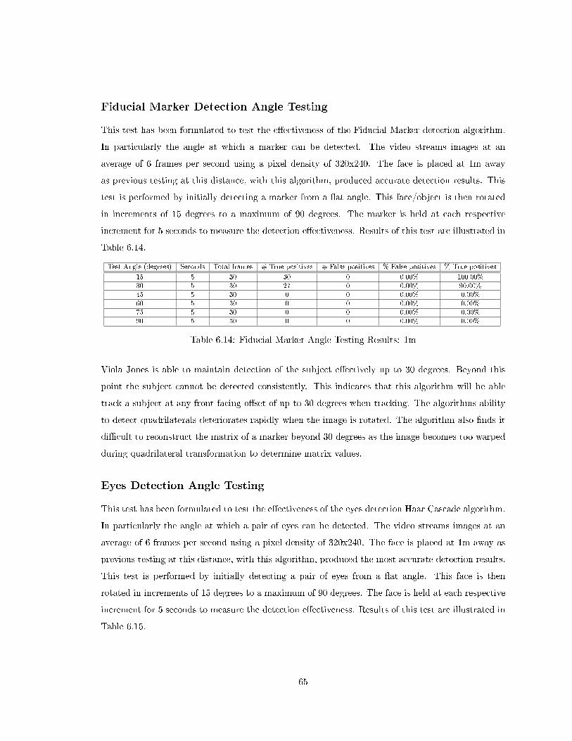
Fiducial Marker Detection Angle Testing
This test has been formulated to test the e�ectiveness of the Fiducial Marker detection algorithm.
In particularly the angle at which a marker can be detected. The video streams images at an
average of 6 frames per second using a pixel density of 320x240. The face is placed at 1m away
as previous testing at this distance, with this algorithm, produced accurate detection results. This
test is performed by initially detecting a marker from a �at angle. This face/object is then rotated
in increments of 15 degrees to a maximum of 90 degrees. The marker is held at each respective
increment for 5 seconds to measure the detection e�ectiveness. Results of this test are illustrated in
Table 6.14.
Test Angle (degrees) Seconds Total frames # True positives # False positives % False positives % True positives
15 5 30 30 0 0.00% 100.00%30 5 30 27 0 0.00% 90.00%45 5 30 0 0 0.00% 0.00%60 5 30 0 0 0.00% 0.00%75 5 30 0 0 0.00% 0.00%90 5 30 0 0 0.00% 0.00%
Table 6.14: Fiducial Marker Angle Testing Results: 1m
Viola Jones is able to maintain detection of the subject e�ectively up to 30 degrees. Beyond this
point the subject cannot be detected consistently. This indicates that this algorithm will be able
track a subject at any front facing o�set of up to 30 degrees when tracking. The algorithms ability
to detect quadrilaterals deteriorates rapidly when the image is rotated. The algorithm also �nds it
di�cult to reconstruct the matrix of a marker beyond 30 degrees as the image becomes too warped
during quadrilateral transformation to determine matrix values.
Eyes Detection Angle Testing
This test has been formulated to test the e�ectiveness of the eyes detection Haar Cascade algorithm.
In particularly the angle at which a pair of eyes can be detected. The video streams images at an
average of 6 frames per second using a pixel density of 320x240. The face is placed at 1m away as
previous testing at this distance, with this algorithm, produced the most accurate detection results.
This test is performed by initially detecting a pair of eyes from a �at angle. This face is then
rotated in increments of 15 degrees to a maximum of 90 degrees. The face is held at each respective
increment for 5 seconds to measure the detection e�ectiveness. Results of this test are illustrated in
Table 6.15.
65
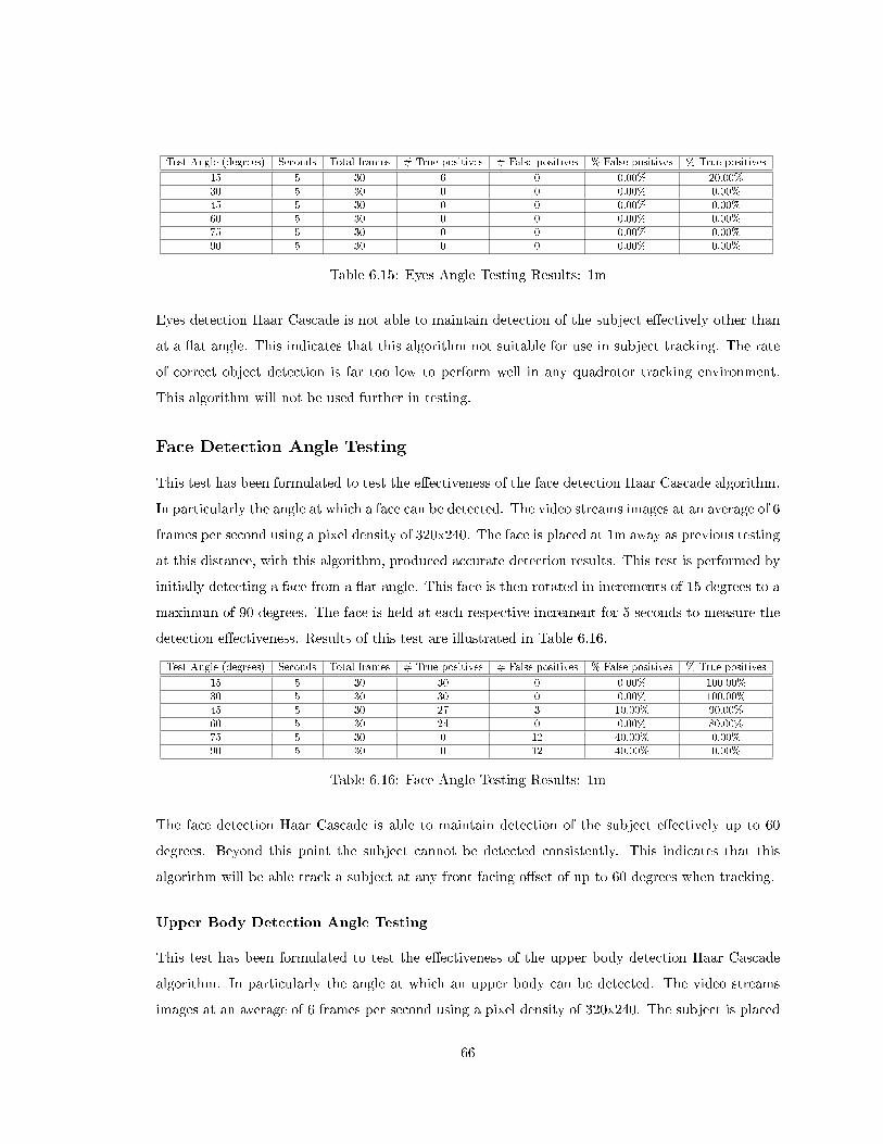
Test Angle (degrees) Seconds Total frames # True positives # False positives % False positives % True positives
15 5 30 6 0 0.00% 20.00%30 5 30 0 0 0.00% 0.00%45 5 30 0 0 0.00% 0.00%60 5 30 0 0 0.00% 0.00%75 5 30 0 0 0.00% 0.00%90 5 30 0 0 0.00% 0.00%
Table 6.15: Eyes Angle Testing Results: 1m
Eyes detection Haar Cascade is not able to maintain detection of the subject e�ectively other than
at a �at angle. This indicates that this algorithm not suitable for use in subject tracking. The rate
of correct object detection is far too low to perform well in any quadrotor tracking environment.
This algorithm will not be used further in testing.
Face Detection Angle Testing
This test has been formulated to test the e�ectiveness of the face detection Haar Cascade algorithm.
In particularly the angle at which a face can be detected. The video streams images at an average of 6
frames per second using a pixel density of 320x240. The face is placed at 1m away as previous testing
at this distance, with this algorithm, produced accurate detection results. This test is performed by
initially detecting a face from a �at angle. This face is then rotated in increments of 15 degrees to a
maximum of 90 degrees. The face is held at each respective increment for 5 seconds to measure the
detection e�ectiveness. Results of this test are illustrated in Table 6.16.
Test Angle (degrees) Seconds Total frames # True positives # False positives % False positives % True positives
15 5 30 30 0 0.00% 100.00%30 5 30 30 0 0.00% 100.00%45 5 30 27 3 10.00% 90.00%60 5 30 24 0 0.00% 80.00%75 5 30 0 12 40.00% 0.00%90 5 30 0 12 40.00% 0.00%
Table 6.16: Face Angle Testing Results: 1m
The face detection Haar Cascade is able to maintain detection of the subject e�ectively up to 60
degrees. Beyond this point the subject cannot be detected consistently. This indicates that this
algorithm will be able track a subject at any front facing o�set of up to 60 degrees when tracking.
Upper Body Detection Angle Testing
This test has been formulated to test the e�ectiveness of the upper body detection Haar Cascade
algorithm. In particularly the angle at which an upper body can be detected. The video streams
images at an average of 6 frames per second using a pixel density of 320x240. The subject is placed
66

at 2.5m away as previous testing at this distance, with this algorithm, produced accurate detection
results. This test is performed by initially detecting an upper body from a �at angle. The upper
body is then rotated in increments of 15 degrees to a maximum of 90 degrees. The upper body is
held at each respective increment for 5 seconds to measure the detection e�ectiveness. Results of
this test are illustrated in Table 6.17.
Test Angle (degrees) Seconds Total frames # True positives # False positives % False positives % True positives
15 5 30 27 3 10.00% 90.00%30 5 30 18 12 40.00% 60.00%45 5 30 15 15 50.00% 50.00%60 5 30 18 12 40.00% 60.00%75 5 30 6 24 80.00% 20.00%90 5 30 6 24 80.00% 20.00%
Table 6.17: Upper Body Angle Testing Results: 1m
The upper body detection Haar Cascade is able to maintain detection of the subject e�ectively up to
60 degrees. Beyond this point the subject cannot be detected consistently. This indicates that this
algorithm will be able track a subject at any front facing o�set of up to 60 degrees when tracking.
6.3 Recognition Results
To assess the e�ectiveness of each of the recognition algorithms, a standard test was devised. Each
algorithm needed to recognise its respective face, object or marker, hence forth known as the subject.
The subject was placed a speci�c distance away from the camera and executed a standard set of
movements. Each algorithm's recognition ability was then assessed according to the number of
frames the subject was detected in (true positives), the number of frames in which false detections
(false positives) were made, the overall percentage of false positives and the overall percentage of
true positives. The following sections will report on the performance of each algorithm and outline
the speci�cs of each test.
6.3.1 Fiducial Marker Recognition Results
The �ducial marker recognition algorithm uses the quadrilateral transformation algorithm and �du-
cial marker matrix reconstruction algorithm to recognise a marker. The goal of this algorithm is to
detect and identify a �ducial marker in a live video stream. The following tests were performed using
the EZ-B robotics API. The subject the test is performed on starts o� directly facing the camera.
This position is held for �ve seconds. The subject then moves to the left and holds this position
for �ve seconds. The subject then moves to the right and holds this position for �ve seconds. The
67
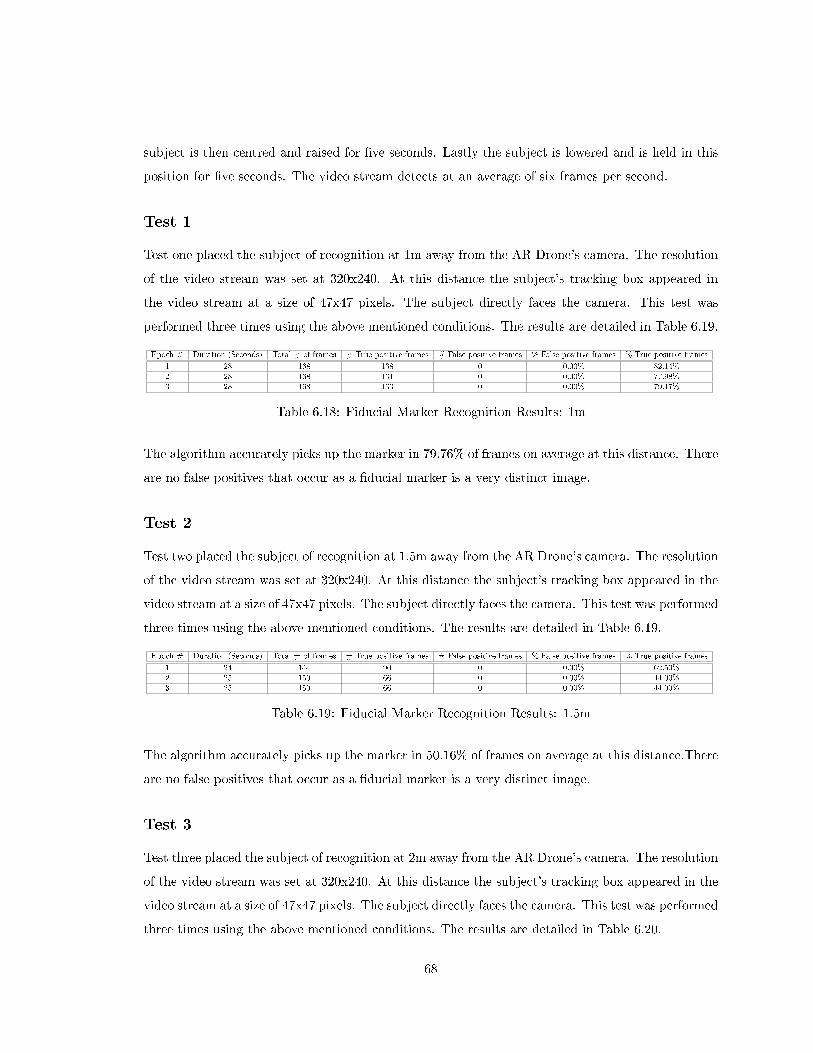
subject is then centred and raised for �ve seconds. Lastly the subject is lowered and is held in this
position for �ve seconds. The video stream detects at an average of six frames per second.
Test 1
Test one placed the subject of recognition at 1m away from the AR Drone's camera. The resolution
of the video stream was set at 320x240. At this distance the subject's tracking box appeared in
the video stream at a size of 47x47 pixels. The subject directly faces the camera. This test was
performed three times using the above mentioned conditions. The results are detailed in Table 6.19.
Epoch # Duration (Seconds) Total # of frames # True positive frames # False positive frames % False positive frames % True positive frames
1 28 168 138 0 0.00% 82.14%2 28 168 131 0 0.00% 77.98%3 28 168 133 0 0.00% 79.17%
Table 6.18: Fiducial Marker Recognition Results: 1m
The algorithm accurately picks up the marker in 79.76% of frames on average at this distance. There
are no false positives that occur as a �ducial marker is a very distinct image.
Test 2
Test two placed the subject of recognition at 1.5m away from the AR Drone's camera. The resolution
of the video stream was set at 320x240. At this distance the subject's tracking box appeared in the
video stream at a size of 47x47 pixels. The subject directly faces the camera. This test was performed
three times using the above mentioned conditions. The results are detailed in Table 6.19.
Epoch # Duration (Seconds) Total # of frames # True positive frames # False positive frames % False positive frames % True positive frames
1 24 144 90 0 0.00% 62.50%2 25 150 66 0 0.00% 44.00%3 25 150 66 0 0.00% 44.00%
Table 6.19: Fiducial Marker Recognition Results: 1.5m
The algorithm accurately picks up the marker in 50.16% of frames on average at this distance.There
are no false positives that occur as a �ducial marker is a very distinct image.
Test 3
Test three placed the subject of recognition at 2m away from the AR Drone's camera. The resolution
of the video stream was set at 320x240. At this distance the subject's tracking box appeared in the
video stream at a size of 47x47 pixels. The subject directly faces the camera. This test was performed
three times using the above mentioned conditions. The results are detailed in Table 6.20.
68
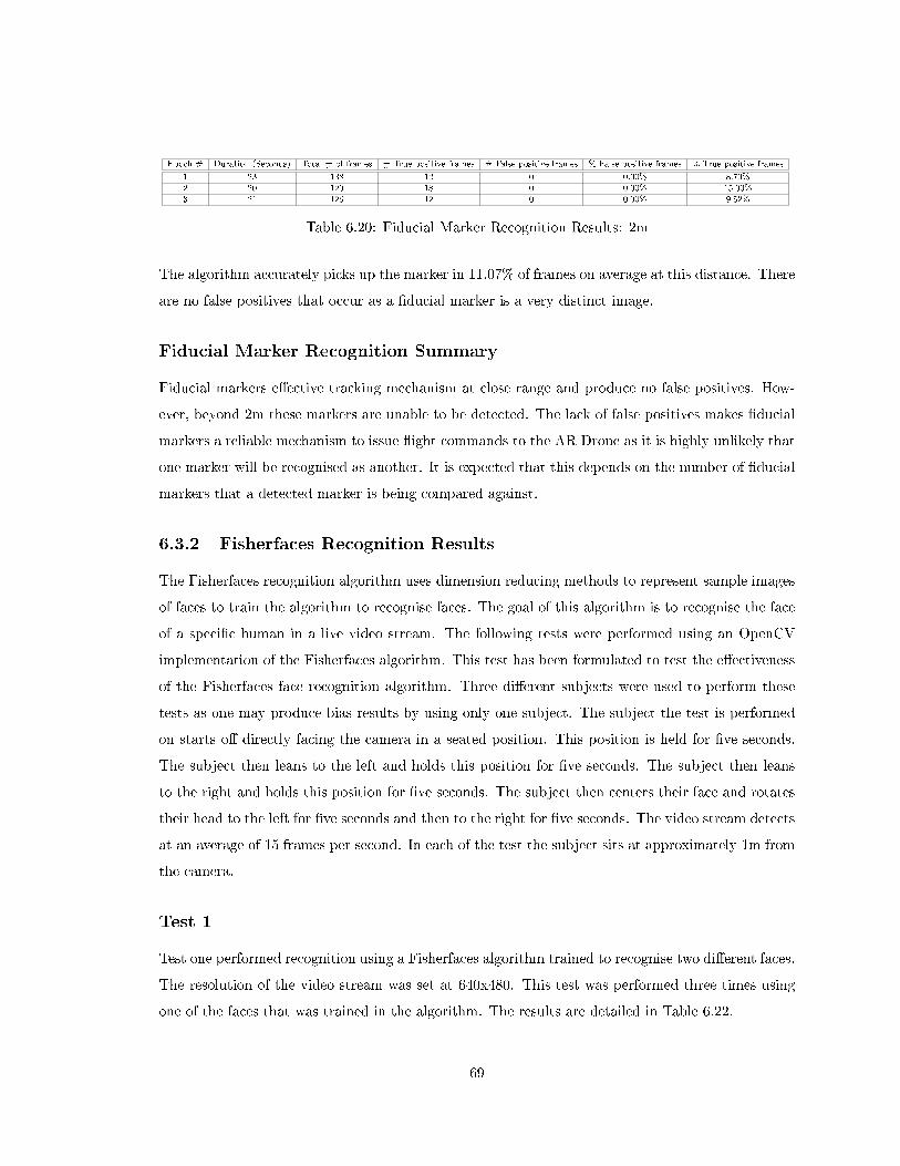
Epoch # Duration (Seconds) Total # of frames # True positive frames # False positive frames % False positive frames % True positive frames
1 23 138 12 0 0.00% 8.70%2 20 120 18 0 0.00% 15.00%3 21 126 12 0 0.00% 9.52%
Table 6.20: Fiducial Marker Recognition Results: 2m
The algorithm accurately picks up the marker in 11.07% of frames on average at this distance. There
are no false positives that occur as a �ducial marker is a very distinct image.
Fiducial Marker Recognition Summary
Fiducial markers e�ective tracking mechanism at close range and produce no false positives. How-
ever, beyond 2m these markers are unable to be detected. The lack of false positives makes �ducial
markers a reliable mechanism to issue �ight commands to the AR Drone as it is highly unlikely that
one marker will be recognised as another. It is expected that this depends on the number of �ducial
markers that a detected marker is being compared against.
6.3.2 Fisherfaces Recognition Results
The Fisherfaces recognition algorithm uses dimension reducing methods to represent sample images
of faces to train the algorithm to recognise faces. The goal of this algorithm is to recognise the face
of a speci�c human in a live video stream. The following tests were performed using an OpenCV
implementation of the Fisherfaces algorithm. This test has been formulated to test the e�ectiveness
of the Fisherfaces face recognition algorithm. Three di�erent subjects were used to perform these
tests as one may produce bias results by using only one subject. The subject the test is performed
on starts o� directly facing the camera in a seated position. This position is held for �ve seconds.
The subject then leans to the left and holds this position for �ve seconds. The subject then leans
to the right and holds this position for �ve seconds. The subject then centers their face and rotates
their head to the left for �ve seconds and then to the right for �ve seconds. The video stream detects
at an average of 15 frames per second. In each of the test the subject sits at approximately 1m from
the camera.
Test 1
Test one performed recognition using a Fisherfaces algorithm trained to recognise two di�erent faces.
The resolution of the video stream was set at 640x480. This test was performed three times using
one of the faces that was trained in the algorithm. The results are detailed in Table 6.22.
69
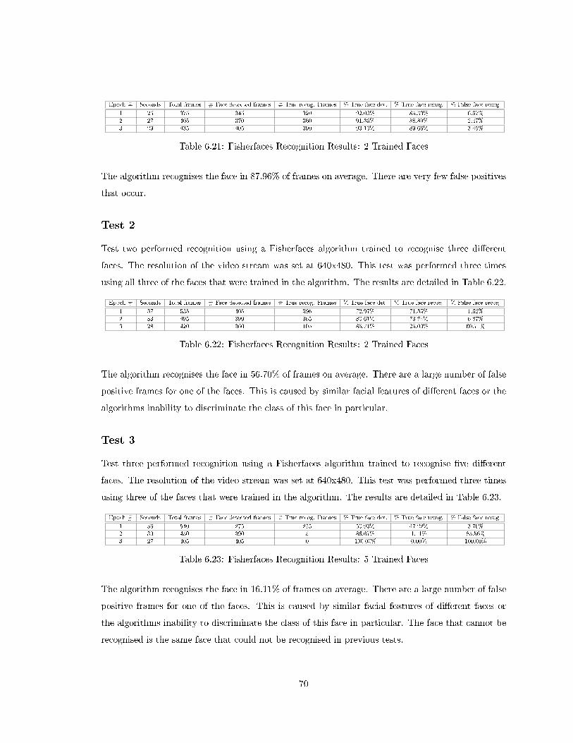
Epoch # Seconds Total frames # Face detected frames # True recog. Frames % True face det. % True face recog. % False face recog.
1 25 375 345 320 92.00% 85.33% 6.67%2 27 405 370 360 91.36% 88.89% 2.47%3 29 435 405 390 93.10% 89.66% 3.45%
Table 6.21: Fisherfaces Recognition Results: 2 Trained Faces
The algorithm recognises the face in 87.96% of frames on average. There are very few false positives
that occur.
Test 2
Test two performed recognition using a Fisherfaces algorithm trained to recognise three di�erent
faces. The resolution of the video stream was set at 640x480. This test was performed three times
using all three of the faces that were trained in the algorithm. The results are detailed in Table 6.22.
Epoch # Seconds Total frames # Face detected frames # True recog. Frames % True face det. % True face recog. % False face recog.
1 37 555 405 396 72.97% 71.35% 1.62%2 33 495 399 365 80.61% 73.74% 6.87%3 28 420 360 105 85.71% 25.00% 60.71%
Table 6.22: Fisherfaces Recognition Results: 2 Trained Faces
The algorithm recognises the face in 56.70% of frames on average. There are a large number of false
positive frames for one of the faces. This is caused by similar facial features of di�erent faces or the
algorithms inability to discriminate the class of this face in particular.
Test 3
Test three performed recognition using a Fisherfaces algorithm trained to recognise �ve di�erent
faces. The resolution of the video stream was set at 640x480. This test was performed three times
using three of the faces that were trained in the algorithm. The results are detailed in Table 6.23.
Epoch # Seconds Total frames # Face detected frames # True recog. Frames % True face det. % True face recog. % False face recog.
1 36 540 275 255 50.93% 47.22% 3.70%2 30 450 390 5 86.67% 1.11% 85.56%3 27 405 405 0 100.00% 0.00% 100.00%
Table 6.23: Fisherfaces Recognition Results: 5 Trained Faces
The algorithm recognises the face in 16.11% of frames on average. There are a large number of false
positive frames for one of the faces. This is caused by similar facial features of di�erent faces or
the algorithms inability to discriminate the class of this face in particular. The face that cannot be
recognised is the same face that could not be recognised in previous tests.
70
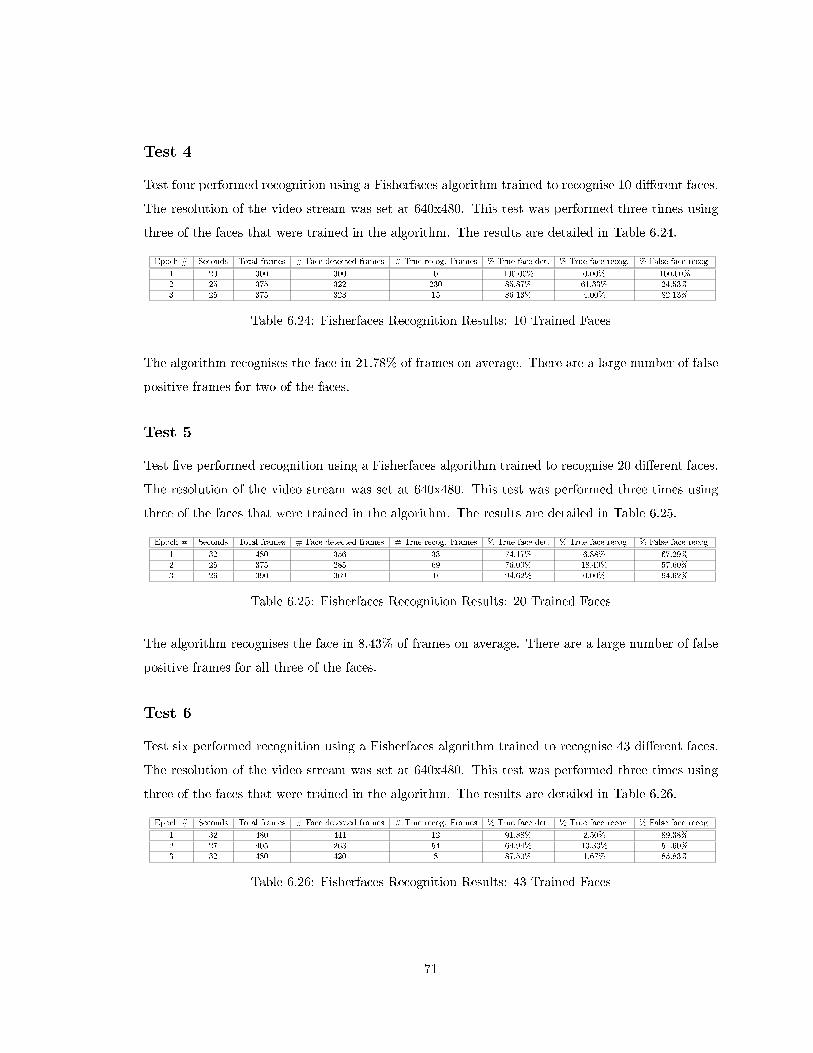
Test 4
Test four performed recognition using a Fisherfaces algorithm trained to recognise 10 di�erent faces.
The resolution of the video stream was set at 640x480. This test was performed three times using
three of the faces that were trained in the algorithm. The results are detailed in Table 6.24.
Epoch # Seconds Total frames # Face detected frames # True recog. Frames % True face det. % True face recog. % False face recog.
1 20 300 300 0 100.00% 0.00% 100.00%2 25 375 322 230 85.87% 61.33% 24.53%3 25 375 323 15 86.13% 4.00% 82.13%
Table 6.24: Fisherfaces Recognition Results: 10 Trained Faces
The algorithm recognises the face in 21.78% of frames on average. There are a large number of false
positive frames for two of the faces.
Test 5
Test �ve performed recognition using a Fisherfaces algorithm trained to recognise 20 di�erent faces.
The resolution of the video stream was set at 640x480. This test was performed three times using
three of the faces that were trained in the algorithm. The results are detailed in Table 6.25.
Epoch # Seconds Total frames # Face detected frames # True recog. Frames % True face det. % True face recog. % False face recog.
1 32 480 356 33 74.17% 6.88% 67.29%2 25 375 285 69 76.00% 18.40% 57.60%3 26 390 369 0 94.62% 0.00% 94.62%
Table 6.25: Fisherfaces Recognition Results: 20 Trained Faces
The algorithm recognises the face in 8.43% of frames on average. There are a large number of false
positive frames for all three of the faces.
Test 6
Test six performed recognition using a Fisherfaces algorithm trained to recognise 43 di�erent faces.
The resolution of the video stream was set at 640x480. This test was performed three times using
three of the faces that were trained in the algorithm. The results are detailed in Table 6.26.
Epoch # Seconds Total frames # Face detected frames # True recog. Frames % True face det. % True face recog. % False face recog.
1 32 480 441 12 91.88% 2.50% 89.38%2 27 405 263 54 64.94% 13.33% 51.60%3 32 480 420 8 87.50% 1.67% 85.83%
Table 6.26: Fisherfaces Recognition Results: 43 Trained Faces
71
The algorithm recognises the face in 8.43% of frames on average. There are a large number of false
positive frames for all three of the faces.
Fisherfaces Recognition Test Summary
This algorithm can recognise a face accurately when there are a few number of faces trained to
the algorithm. The number of false recognitions that occur increase rapidly as the number of faces
trained increases. The algorithm manages to detect a face with the same accuracy as the face
detection Haar Cascade. The test results suggest that one face may produce very di�erent results
from another under the same training and testing conditions. This can be caused by a large similarity
in facial features in di�erent faces or by the algorithms inability to distinguish a face class from a set
of others. The Fisherfaces algorithm is not used during tracking testing owing to the high number
of false positives produced. The algorithm could be improved on by adding more sample images to
the training data or by determining the optimal lighting conditions in which sample images should
be taken to better train the Fisherfaces algorithm.
6.4 Tracking testing
To test the capability of each tracking algorithm during �ight, a standard �ight pattern was devised
as a basis for algorithm comparrison. The most successful four algorithms in detection, angle and
recognition testing were used to test tracking. These algorithms are were the Viola Jones, CamShift,
Fiducial marker recognition and the upper body detection Haar Cascade. Each algorithm either
tracks a face, object or marker which is referred to as the subject. The subject of each test is moved
so that the �ight pattern manoeuvres of the drone are as follows:
1. Take o�.
2. Detect the subject.
3. Fly approximately 1-3 metres to the subject. Distance depends on algorithm capabilities.
4. Stop before colliding with the subject.
5. Track the subject as it circles the drone, completing a 180 degree rotation.
6. Follow the subject as it moves 3 metres away from the drone.
7. Adjust altitude as the subject ascends, then descends.
72
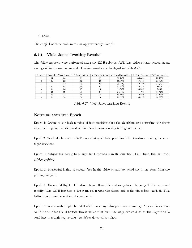
8. Land.
The subject of these tests moves at approximately 0.5m/s.
6.4.1 Viola Jones Tracking Results
The following tests were performed using the EZ-B robotics API. The video stream detects at an
average of six frames per second. Tracking results are displayed in Table 6.27.
Epoch # Seconds Total frames # True positives # False positives % Overall detection % True Positives % False postives
1 14 84 39 30 82.14% 46.43% 35.71%2 21 126 72 15 69.05% 57.14% 11.90%3 7 42 25 15 95.24% 59.52% 35.71%4 25 150 70 13 55.33% 46.67% 8.67%5 6 36 12 3 41.67% 33.33% 8.33%6 24 144 78 15 64.58% 54.17% 10.42%7 9 54 39 6 83.33% 72.22% 11.11%8 9 54 36 9 83.33% 66.67% 16.67%
Table 6.27: Viola Jones Tracking Results
Notes on each test Epoch
Epoch 1: Owing to the high number of false positives that the algorithm was detecting, the drone
was executing commands based on non-face images, causing it to go o� course.
Epoch 2: Tracked a face with e�ectiveness but again false positives led to the drone making incorrect
�ight decisions.
Epoch 3: Subject lost owing to a large �ight correction in the direction of an object that returned
a false positive.
Epoch 4: Successful �ight. A second face in the video stream attracted the drone away from the
primary subject.
Epoch 5: Successful �ight. The drone took o� and turned away from the subject but recovered
rapidly. The EZ B lost the socket connection with the drone and so the video feed crashed. This
halted the drone's execution of commands.
Epoch 6: A successful �ight but still with too many false positives occurring. A possible solution
could be to raise the detection threshold so that faces are only detected when the algorithm is
con�dent to a high degree that the object detected is a face.
73
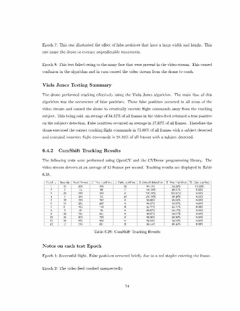
Epoch 7: This test illustrated the e�ect of false positives that have a large width and height. This
can cause the drone to execute unpredictable movements.
Epoch 8: This test failed owing to the many face that were present in the video stream. This caused
confusion in the algorithm and in turn caused the video stream from the drone to crash.
Viola Jones Testing Summary
The drone performed tracking e�ectively using the Viola Jones algorithm. The main �aw of this
algorithm was the occurrence of false positives. These false positives occurred in all areas of the
video stream and caused the drone to erratically execute �ight commands away from the tracking
subject. This being said, an average of 54.52% of all frames in the video feed returned a true positive
on the subjects detection. False positives occurred on average in 17.32% of all frames. Therefore the
drone executed the correct tracking �ight commands in 75.89% of all frames with a subject detected
and executed incorrect �ight commands in 24.10% of all frames with a subject detected.
6.4.2 CamShift Tracking Results
The following tests were performed using OpenCV and the CVDrone programming library. The
video stream detects at an average of 15 frames per second. Tracking results are displayed in Table
6.28.
Epoch # Seconds Total frames # True positives # False positives % Overall detection % True Positives % False postives
1 15 225 185 32 96.44% 82.22% 14.22%2 5 75 68 7 100.00% 90.67% 9.33%3 39 585 585 0 100.00% 100.00% 0.00%4 7 105 95 10 100.00% 90.48% 9.52%5 19 285 267 0 93.68% 93.68% 0.00%6 14 210 207 0 98.57% 98.57% 0.00%7 31 465 443 0 95.27% 95.27% 0.00%8 3 45 30 0 66.67% 66.67% 0.00%9 50 750 680 0 90.67% 90.67% 0.00%10 55 825 795 0 96.36% 96.36% 0.00%11 58 870 802 0 92.18% 92.18% 0.00%12 47 705 680 0 96.45% 96.45% 0.00%
Table 6.28: CamShift Tracking Results
Notes on each test Epoch
Epoch 1: Successful �ight. False positives occurred brie�y due to a red stapler entering the frame.
Epoch 2: The video feed crashed unexpectedly.
74
Epoch 3: Successful �ight. No false detections. Altitude �ight adjustments were disabled to allow
for a more steady �ight.
Epoch 4: The video stream was delayed in arriving at the client terminal and so tracking commenced
mid-�ight instead of at take-o�. The drone successfully maintained a calculated distance from the
subject and tracked the subject successfully. A false positive occurred on a pair of red shoes in the
environment for a short time.
Epoch 5: Successful �ight. Flight was slightly unstable as over corrections in altitude caused the
drone to "bounce" up and down. The video stream crashed possibly owing to the drone activating
"emergency mode" owing to unstable �ight. Emergency mode cuts power to the engines and halts
the reception and transmission of AT Commands, NavData and video stream.
Epoch 6: Again the video stream was late in arriving at the client terminal. However, once it started,
tracking commenced with stability.
Epoch 7: Successful �ight. The drone exhibited a "bounce" when executing the Yaw movement but
stabilised after 3 seconds. Performed altitude adjustments smoothly.
Epoch 8: The drone cut power to the engines abruptly owing to batter power being low. The drone
attempted to take o� again but was unable to owing to a shift in the indoor hull that hindered the
movement of the rotors.
Epoch 9: Successful �ight. Recovered the image of the ball when the ball was removed from the
video stream. Performed altitude adjustments smoothly.
Epoch 10: Successful �ight. Maintained distance from object well. Exhibited bounce in the Yaw
movement but corrected after 2 seconds.
Epoch 11: Successful �ight. Maintained distance from object well. Exhibited bounce in the Yaw
movement but corrected after 2 seconds.
Epoch 12: Successful �ight. Maintained distance from object well. Exhibited bounce in the Yaw
movement but corrected after 2 seconds.
75

CamShift Testing Summary
The drone performed tracking extremely e�ectively using the CamShift algorithm. The main �aw
of this algorithm was the occurrence of �bounce� in drone movements. This was owing to �ight
movements that over corrected the drone's position according to which quadrant the subject was
in. This caused brief movements of instability during �ight. A very low number of frames returned
false positives and this only occurred when similarly coloured objects entered the frame. An average
of 91.10% of all frames in the video feed returned a true positive on the subject's detection. False
positives occurred on average in 2.76% of all frames. Therefore the drone executed the correct
tracking �ight commands in 97.06% of all frames with a subject detected and executed incorrect
�ight commands in 2.93% of all frames with a subject detected.
6.4.3 Fiducial Marker Tracking Results
The following tests were performed using the EZ-B robotics API. The video stream detects at an
average of six frames per second. Tracking results are displayed in Table 6.29.
Epoch # Seconds Total frames # True positives # False positives % Overall detection % True Positives % False postives
1 11 66 30 0 45.45% 45.45% 0.00%2 7 42 28 0 66.67% 66.67% 0.00%3 7 42 28 0 66.67% 66.67% 0.00%4 9 54 24 0 44.44% 44.44% 0.00%5 22 132 82 0 62.12% 62.12% 0.00%6 15 90 24 0 26.67% 26.67% 0.00%7 24 144 60 0 41.67% 41.67% 0.00%8 7 42 12 0 28.57% 28.57% 0.00%9 17 102 60 0 58.82% 58.82% 0.00%10 24 144 84 0 58.33% 58.33% 0.00%11 30 180 102 0 56.67% 56.67% 0.00%12 30 180 84 0 46.67% 46.67% 0.00%13 21 126 90 0 71.43% 71.43% 0.00%
Table 6.29: Fiducial Marker Tracking Results
Notes on each test Epoch
Epoch 1: The drone took o� using marker 1 as programmed. The drone began executing a pre-
programmed search pattern initiated by the recognition of marker 2. Crashed into furniture.
Epoch 2: The drone took o� using marker 1 as programmed. The drone began to track marker 3
but the video stream crashed.
Epoch 3: The drone took o� using marker 1 as programmed. The drone began to track marker 3
but the video stream crashed.
76
Epoch 4: The drone took o� using marker 1 as programmed. The drone began executing a pre-
programmed search pattern initiated by the recognition of marker 2. Crashed into furniture.
Epoch 5: The drone took o� using marker 1 as programmed. The drone began tracking marker 3.
Due to the delay in marker detection time, AT commands were being sent to the drone infrequently.
This resulted in marker detection points in the video feed being far apart. Crashed into furniture.
Epoch 6: The drone is unable to detect or recognise markers beyond approximately 2m.
Epoch 7: Successful �ight. However the algorithm struggles to pick up a marker moving faster than
approximately 1m/s.
Epoch 8: Steady detection but crashed into furniture owing to the drones inertial movement.
Epoch 9: Successful �ight. However, the grid tracking lines seem to be causing to the drone to
execute rotation commands too sensitively for the distance that the �ducial marker can be tracked
at.
Epoch 10: Successful �ight. Performs rotation smoothly. Distance maintenance from the marker is
miscalculating.
Epoch 11: Successful �ight. Performs rotation smoothly. Distance maintenance from the marker is
miscalculating.
Epoch 12: Successful �ight. Performs rotation smoothly. Distance maintenance from the marker is
miscalculating.
Epoch 13: Successful �ight. Performs rotation smoothly. Performs altitude changes smoothly. Delay
in marker detection evident.
Fiducial Marker Testing Summary
The drone performed tracking erratically using the �ducial marker tracking algorithm. The main
�aw of this algorithm was the delay in marker recognition. This a�ected the speed at which a
moving marker could be recognised. The algorithm produced no false positives which ensured that
only correct �ight commands were executed. An average of 51.86% of all frames in the video feed
77
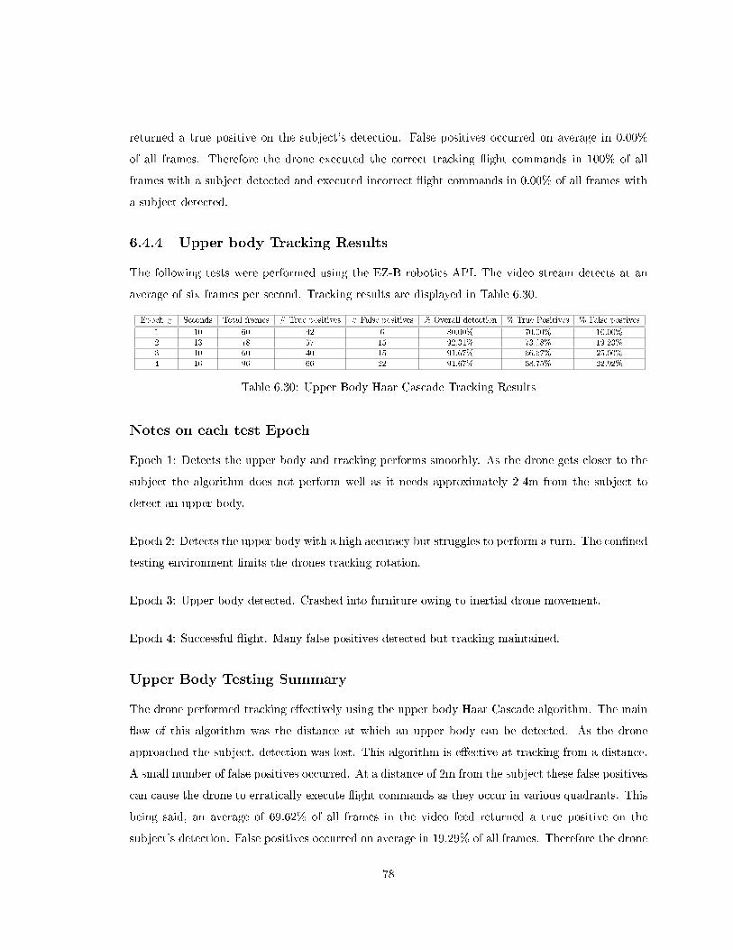
returned a true positive on the subject's detection. False positives occurred on average in 0.00%
of all frames. Therefore the drone executed the correct tracking �ight commands in 100% of all
frames with a subject detected and executed incorrect �ight commands in 0.00% of all frames with
a subject detected.
6.4.4 Upper body Tracking Results
The following tests were performed using the EZ-B robotics API. The video stream detects at an
average of six frames per second. Tracking results are displayed in Table 6.30.
Epoch # Seconds Total frames # True positives # False positives % Overall detection % True Positives % False postives
1 10 60 42 6 80.00% 70.00% 10.00%2 13 78 57 15 92.31% 73.08% 19.23%3 10 60 40 15 91.67% 66.67% 25.00%4 16 96 66 22 91.67% 68.75% 22.92%
Table 6.30: Upper Body Haar Cascade Tracking Results
Notes on each test Epoch
Epoch 1: Detects the upper body and tracking performs smoothly. As the drone gets closer to the
subject the algorithm does not perform well as it needs approximately 2-4m from the subject to
detect an upper body.
Epoch 2: Detects the upper body with a high accuracy but struggles to perform a turn. The con�ned
testing environment limits the drones tracking rotation.
Epoch 3: Upper body detected. Crashed into furniture owing to inertial drone movement.
Epoch 4: Successful �ight. Many false positives detected but tracking maintained.
Upper Body Testing Summary
The drone performed tracking e�ectively using the upper body Haar Cascade algorithm. The main
�aw of this algorithm was the distance at which an upper body can be detected. As the drone
approached the subject, detection was lost. This algorithm is e�ective at tracking from a distance.
A small number of false positives occurred. At a distance of 2m from the subject these false positives
can cause the drone to erratically execute �ight commands as they occur in various quadrants. This
being said, an average of 69.62% of all frames in the video feed returned a true positive on the
subject's detection. False positives occurred on average in 19.29% of all frames. Therefore the drone
78
executed the correct tracking �ight commands in 78.30% of all frames with a subject detected and
executed incorrect �ight commands in 21.69% of all frames with a subject detected.
6.5 Summary
The results from tests performed on the AR Drone were positive and highlighted many of the
strengths and weaknesses that need to be considered when implementing a detection, recognition
and tracking system for the drone. Many of the algorithms encountered problems with the detection
of false positives and this impeded the drone's ability to track a subject completely accurately.
There were limitations on the distances at which algorithms could successfully track their subjects.
This limitation is a consequence many factors such as image pixel density, frame frequency and the
lighting in a tracking environment. It is expected that the drone's capable tracking distances would
increase by making use of a higher quality camera and algorithms with more elaborate detection
techniques. The inertial movement of the drone caused some �ight test results to vary especially
owing to the small size of the testing environment. On a larger scale, the drone's inertial movement
is expected to become negligible to an extent. The relatively few number of angle that subjects
were able to be detected at required tests to be performed in fairly ideal conditions. Advanced
searching algorithms could be employed to assess an environment at as many angles as possible to
deal with this limitation. When performing recognition, there was a small amount of time needed to
process a detected subject. This led to noticable delays in tracking command execution and limited
the speed at which an object was able to move whilst successfully performing tracking. Toward
the end of testing, the drone's components became slightly damaged from test �ight crashes and
made some �ight movements unpredictable. The drone was successfully able to detect, recognise
and track various subjects during tests and provided useful insight into the AR Drones capability
and limitations.
79
Chapter 7
Conclusion
The system created performs the autonomous functions of target detection, recognition and tracking
using the Parrot AR Drone. Various methods and algorithms were used to implement each function
and the capability of these algorithms was tested rigorously. Each algorithms capable distance, angle
of detection, accuracy and tracking performance was assessed to determine whether using a drone
to perform these functions was conceptually feasible. Various strengths and limitations of the AR
Drone and the algorithms used to implement each of the functions were identi�ed. The AR Drone
was the most suitable aerial vehicle to implement this system as it allowed each of the algorithms
to be tested indoors in a controlled environment. This allowed the algorithms to be tested in an
environment devoid of many outdoor factors such as wind, condensation and lighting changes. The
AR Drones ability to hover made it possible to perform tests in a small and monitorable space which
would not be possible using �xed wing drones.
The APIs that were used were chosen according to how well they implemented an algorithm. It
was found that one API could implement a certain algorithm e�ectively but encountered di�culties
with others. The tools, functions and programming languages of each API determined its capabilities
and so di�erent APIs were used to implement various algorithms.
A few challenges were encountered when implementing and testing algorithms. The video feed
from the AR Drone would occasionally crash owing to the drone venturing too far from the client PC
or from socket exceptions. The socket exceptions caused the existing video feed connection to the
drone to be closed by the remote host and so the visual capabilities of the drone were periodically
lost. The drone's components became slightly damaged towards the end of testing which caused
drone to move unpredictable at times.
80
The results obtained from testing showed that the Camshift and Viola Jones face detection algo-
rithms were the most e�ective in terms of distance capabilities, e�ective detection angles, accuracy
and tracking performance. Fiducial marker recognition allowed the drone to e�ectively execute pre-
de�ned �ight scripts but was not able to recognise markers from distances beyond approximately
2m. The Haar-Cascade algorithms performed relatively well with the exception of the eye detection
which produced very ine�ective test results. Fisherfaces was able to recognise a face with relative
accuracy but this accuracy declined rapidly as the sample set of trained faces became larger.
The system was successfully able to evaluate the capabilities of various algorithms and demon-
strated that a micro UAV such as the Parrot AR Drone is capable of performing autonomous de-
tection, recognition and tracking during �ight. The requirements detailed in Chapter 1 are deemed
to have been successfully ful�lled.
7.1 Future Work
One could elaborate on this system in various ways. Firstly, one could make use of a camera that
can capture video at a higher pixel density and frame rate. This would increase the accuracy of
detection as well as the distance of detection. Objects that are detected at a distance could be
zoomed in on for more accurate tracking and recognition. To further improve the detection and
tracking capabilities of the drone, a function could be created that selects the most appropriate
tracking algorithm according to the drones environment. The drone could attempt to detect a
human initially by using face detection. Should this prove unsuccessful the drone could swap to
an upper body or full body Haar Cascade detection algorithm. The would enable the drone to
constantly swap between algorithms to maintain a lock on the target.
3D mapping could be used to create an image of the immediate environment so that the drone
could autonomously navigate around obstacles on its �ight path whilst tracking a target. Currently
the drone requires a client application to perform image processing and send �ight commands. The
drone communicates with this client application via Wi-Fi and so there is a limit on how far the
drone can travel from its client device. Placing an on board computer such as the Raspberry Pi on
the drone would eliminate this limitation. Finally, the AR Drone is only able to operate outdoors in
clam weather conditions. A more robust drone design would be needed for the drone to handle strong
winds or rain. A more robust drone such as a hexrotor could be used to handle these conditions.
This would also allow the drone to carry a heavier payload such as additional batteries, sensors and
on board computer.
81

Bibliography
Achtelik, Markus, Bachrach, Abraham, He, Ruijie, Prentice, Samuel, & Roy, Nicholas. 2009. Stereo
vision and laser odometry for autonomous helicopters in GPS-denied indoor environments. In:
SPIE Defense, Security, and Sensing. International Society for Optics and Photonics.
Allen, John G, Xu, Richard YD, & Jin, Jesse S. 2004. Object tracking using camshift algorithm and
multiple quantized feature spaces. Pages 3�7 of: Proceedings of the Pan-Sydney area workshop
on Visual information processing. Australian Computer Society, Inc.
AR.Drone. 2009. ARDrone API. Online. Available from: https://projects.ardrone.org/. Ac-
cessed on 31 Oct 2013.
AR.Drone2.0. 2013. Repair Your AR.Drone. Online. Available from: http://ardrone2.parrot.
com/repair-your-ardrone/. Accessed on 31 Oct 2013.
Arjomandi, Maziar, Agostino, S, Mammone, M, Nelson, M, & Zhou, T. 2007. Classi�cation of
Unmanned Aerial Vehicles. The University of Adelaide, Australia.
Beard, Randal W, Kingston, Derek, Quigley, Morgan, Snyder, Deryl, Christiansen, Reed, Johnson,
Walt, McLain, Timothy, & Goodrich, Michael. 2005. Autonomous vehicle technologies for small
�xed-wing UAVs. Journal of Aerospace Computing, Information, and Communication, 2(1), 92�
108.
Belhumeur, Peter N., Hespanha, João P, & Kriegman, David J. 1997. Eigenfaces vs. �sherfaces:
Recognition using class speci�c linear projection. IEEE Transactions on Pattern Analysis and
Machine Intelligence, 19(7), 711�720.
Belisarius. 2011. Image Segmentation using Mean Shift explained. On-
line. Available from: http://stackoverflow.com/questions/4831813/
image-segmentation-using-mean-shift-explained. Accessed on 31 Oct 2013.
82
Biber, Peter, Andreasson, Henrik, Duckett, Tom, & Schilling, Andreas. 2004. 3D modeling of indoor
environments by a mobile robot with a laser scanner and panoramic camera. Pages 3430�3435
of: Proceedings IEEE/RSJ International Conference on Intelligent Robots and Systems.(IROS
2004)., vol. 4. IEEE.
Bills, Cooper, Chen, Joyce, & Saxena, Ashutosh. 2011. Autonomous MAV �ight in indoor environ-
ments using single image perspective cues. Pages 5776�5783 of: IEEE international conference
on Robotics and automation (ICRA 2011). IEEE.
Bradski, Gary R. 1998. Real time face and object tracking as a component of a perceptual user
interface. Pages 214�219 of: Proceedings of IEEE Workshop on Applications of Computer Vision
(WACV 1998). IEEE.
Bristeau, Pierre-Jean, Callou, François, Vissière, David, Petit, Nicolas, et al. 2011. The Navigation
and Control technology inside the AR.Drone micro UAV. Pages 1477�1484 of: World Congress,
vol. 18.
Cambridge, AT&T Laboratories. 2002. The Database of Faces. Online. Available from: http://
www.cl.cam.ac.uk/research/dtg/attarchive/facedatabase.html. Accessed on 8 Aug 2013.
Çelik, Koray, Chung, Soon-Jo, Clausman, Matthew, & Somani, Arun K. 2009. Monocular vision
SLAM for indoor aerial vehicles. Pages 1566�1573 of: IEEE/RSJ International Conference on
Intelligent Robots and Systems. (IROS 2004). IEEE.
Cherian, Anoop, Andersh, Jonathan, Morellas, Vassilios, Papanikolopoulos, Nikolaos, & Mettler,
Bernard. 2009. Autonomous altitude estimation of a UAV using a single onboard camera. Pages
3900�3905 of: IEEE/RSJ International Conference on Intelligent Robots and Systems. (IROS
2009). IEEE.
Courbon, Jonathan, Mezouar, Youcef, Guenard, Nicolas, & Martinet, Philippe. 2009. Visual nav-
igation of a quadrotor aerial vehicle. Pages 5315�5320 of: IEEE/RSJ International Conference
on Intelligent Robots and Systems.(IROS 2009). IEEE.
Crew, Flight. 2013. Flight Crew-Fixed Wing Vs Rotary UAV. Online. Available from: http:
//www.hse-uav.com/fixed_wing_vs_rotary_wing_uav.htm. Accessed on 19 May 2013.
Danko, Todd W, Kellas, Andreas, & Oh, Paul Y. 2005. Robotic rotorcraft and perch-and-stare:
sensing landing zones and handling obscurants. Pages 296�302 of: Proceedings of the 12th Inter-
national Conference on Advanced Robotics.(ICAR 2005). IEEE.
83
de Souza, Cesar. 2012. Haar-feature Object Detection in C. Online. Available from: http://www.
codeproject.com/Articles/441226/Haar-feature-Object-Detection-in-Csharp. Accessed
on 31 Oct 2013.
Dijkshoorn, Nick. 2012. Simultaneous localization and mapping with the ar. drone. Ph.D. thesis,
Universiteit van Amsterdam.
Greensted, Dr. Andrew. 2010. Otsu Thresholding. Online. Available from: http://www.
labbookpages.co.uk/software/imgProc/otsuThreshold.html. Accessed on 31 Oct 2013.
Hewitt, Robin. 2007. Face Recognition With Eigenface. Online. Available from: http://www.
cognotics.com/opencv/servo_2007_series/part_4/page_2.html. Accessed on 31 Oct 2013.
Hwang, Wonjun, Kim, Tae-Kyun, & Kee, Seokcheol. 2004. LDA with subgroup PCA method for
facial image retrieval. Pages 21�23 of: The 5th International Workshop on Image Analysis for
Multimedia Interactive Services (WIAMIS 2004).
Isaac Gerg, Adam Ickes, Jamie McCulloch. 2003. CamShift Tracking Algorithm. Online. Available
from: http://www.gergltd.com/cse486/project5/. Accessed on 31 Oct 2013.
Johnson, Neil G. 2008. Vision-assisted control of a hovering air vehicle in an indoor setting. Ph.D.
thesis, Brigham Young University. Department of Mechanical Engineering.
Kendoul, Farid, Fantoni, Isabelle, & Nonami, Kenzo. 2009. Optic �ow-based vision system for au-
tonomous 3D localization and control of small aerial vehicles. Robotics and Autonomous Systems,
57(6), 591�602.
Kirillov, Andrew. 2010. Glyph's recognition. Online. Available from: http://www.aforgenet.com/
articles/glyph_recognition/. Accessed on 31 Oct 2013.
Mayer, Jane. 2009. The predator war. The New Yorker, 85, 36�45.
Mejias, Luis, Campoy, Pascual, Usher, Kane, Roberts, Jonathan, & Corke, Peter. 2006. Two seconds
to touchdown-vision-based controlled forced landing. Pages 3527�3532 of: IEEE/RSJ Interna-
tional Conference on Intelligent Robots and Systems. IEEE.
Moore, Richard James Donald, Thurrowgood, Saul, Bland, Daniel, Soccol, Dean, & Srinivasan,
Mandyam V. 2009. A stereo vision system for UAV guidance. Pages 3386�3391 of: IEEE/RSJ
International Conference on Intelligent Robots and Systems.(IROS 2009). IEEE.
84

Mori, Ryosuke, Hirata, Kenichi, & Kinoshita, Takuya. 2007. Vision-based guidance control of a
small-scale unmanned helicopter. Pages 2648�2653 of: IEEE/RSJ International Conference on
Intelligent Robots and Systems.(IROS 2007). IEEE.
Morris, Stephen J. 1997. Design and �ight test results for micro-sized �xed-wing and VTOL aircraft.
In: Proceedings of the First Internation Conference on Emerging Technologies for Micro Air
Vehicles, Atlanta, GA. Citeseer.
Nicoud, J-D, & Zu�erey, J-C. 2002. Toward indoor �ying robots. Pages 787�792 of: IEEE/RSJ
International Conference on Intelligent Robots and Systems., vol. 1. IEEE.
OpenCV. 2013a. OpenCV Haar-Cascades. Online. Available from: https://opencvlibrary.svn.
sourceforge.net/svnroot/opencvlibrary/tags/latest_tested_snapshot/opencv/data/
haarcascades. Accessed on 31 Oct 2013.
OpenCV. 2013b. OpenCV Software Library. Online. Available from: http://opencv.org. Accessed
on 31 Oct 2013.
Portal, João Víctor. 2011. A Java autopilot for parrot AR drone designed with DiaSpec. M.Phil.
thesis, Universidade Federal Do Rio Grande Do Sul.
puku0x. 2012. CV Drone. Online. Available from: https://github.com/puku0x/cvdrone. Accessed
on 31 Oct 2013.
Roberts, James F, Stirling, Timothy S, Zu�erey, J-C, & Floreano, Dario. 2009. 2.5 D infrared
range and bearing system for collective robotics. Pages 3659�3664 of: IEEE/RSJ International
Conference on Intelligent Robots and Systems.(IROS 2009). IEEE.
Soundararaj, Sai Prashanth, Sujeeth, Arvind K, & Saxena, Ashutosh. 2009. Autonomous indoor
helicopter �ight using a single onboard camera. Pages 5307�5314 of: IEEE/RSJ International
Conference on Intelligent Robots and Systems, 2009. (IROS 2009). IEEE.
Stephane Piskorski, Nicolas Brulez, Pierre Eline. 2011. AR.Drone Developer Guide SDK 1.7. Sdk
1.7 edn. Parrot.
Sures, DJ. Online. Available from: http://www.ez-robot.com/EZ-Builder/. Accessed on 31 Oct
2013.
85
Tournier, Glenn P, Valenti, Mario, How, Jonathan P, & Feron, Eric. 2006. Estimation and control
of a quadrotor vehicle using monocular vision and moire patterns. Pages 21�24 of: Navigation
and Control Conference and Exhibit on AIAA Guidance.
Turk, Matthew, & Pentland, Alex. 1991. Eigenfaces for recognition. Journal of cognitive neuro-
science, 3(1), 71�86.
Viola, Paul, Jones, Michael J, & Snow, Daniel. 2005. Detecting pedestrians using patterns of motion
and appearance. International Journal of Computer Vision, 63(2), 153�161.
Wagner, Philipp. 2012. Face Recognition with Python. Online. Available from: http://www.
bytefish.de/blog/fisherfaces/. Accessed on 31 Oct 2013.
Zingg, Simon, Scaramuzza, Davide, Weiss, Stephan, & Siegwart, Roland. 2010. MAV navigation
through indoor corridors using optical �ow. Pages 3361�3368 of: Robotics and Automation
(ICRA), 2010 IEEE International Conference on. IEEE.
86