lable at ScienceDirect

Environmental Modelling & Software 26 (2011) 751e760

Contents lists avai

Environmental Modelling & Software

journal homepage: www.elsevier .com/locate/envsoft

An environmental decision support system for spatial assessment and selectiveremediation

Robert N. Stewart a,b, S. Thomas Purucker c,*aDepartment of Ecology and Evolutionary Biology, University of Tennessee, Knoxville, TN 37996, USAbComputational Sciences and Engineering Division, Oak Ridge National Laboratory, P.O. Box 2008, Oak Ridge, TN 37831, USAcOffice of Research and Development, U.S. Environmental Protection Agency, 960 College Station Road, Athens, GA 30605, USA

a r t i c l e i n f o

Article history:Received 21 April 2010Received in revised form20 December 2010Accepted 23 December 2010Available online 3 February 2011

Keywords:Environmental decision support softwareGeostatisticsSample designRisk assessmentSelective remediation

* Corresponding author.E-mail address: purucker.tom@gmail.com (S.T. Pur

1364-8152/$ e see front matter Published by Elsevierdoi:10.1016/j.envsoft.2010.12.010

a b s t r a c t

Spatial Analysis and Decision Assistance (SADA) is a Windows freeware program that incorporates spatialassessment tools for effective environmental remediation. The software integrates modules for GIS,visualization, geospatial analysis, statistical analysis, human health and ecological risk assessment, cost/benefit analysis, sampling design, and decision support. SADA began as a simple tool for integrating riskassessment with spatial modeling tools. It has since evolved into a freeware product primarily targetedfor spatial site investigation and soil remediation design, though its applications have extended intomany diverse environmental disciplines that emphasize the spatial distribution of data. Because of thevariety of algorithms incorporated, the user interface is engineered in a consistent and scalable mannerto expose additional functionality without a burdensome increase in complexity. The scalable environ-ment permits it to be used for both application and research goals, especially investigating spatial aspectsimportant for estimating environmental exposures and designing efficient remedial designs. The result isa mature infrastructure with considerable environmental decision support capabilities. We provide anoverview of SADA’s central functions and discuss how the problem of integrating diverse models ina tractable manner was addressed.

Published by Elsevier Ltd.

Software availability

SADA is freeware: binaries for the full-featured installation files,documentation, databases, and examples are available forfree download at: http://www.tiem.utk.edu/wsada/index.shtml. Minimum resolution is 1024�768 with 16million colors (for 3-D viewing); processor should bea minimum Pentium 3 processor with 800 GHz, 512 MBRAM, and 800 MB hard disk space available for installa-tion. The interface is constructed in VB.Net and leveragesdynamic link libraries for algorithms constructed in otherlanguages, including C and Fortran.

1. Introduction

Visualization is a key component of modern site assessments;however, visualization combined with spatial data analysis andassessment algorithms requiresprogramming skills andbudgetsnot

ucker).

Ltd.

always available for site assessments. These assessments require theintegrated use of tools from multiple disciplines; includingGeographic Information Systems (GIS), sample design, statistics,data management, two- and three-dimensional visualization,spatial modeling, uncertainty analysis, risk assessment, remedialdesign, and cost/benefit analysis. These diverse capabilities mustthen be used together in a coherent, defensible, repeatable decisionprocess (Matott et al., 2009). Generally, this algorithmic integrationis achieved through highly flexible implementations that requiresignificant programming capability (e.g., command-line interface ofRwith contributedpackages (RDevelopmentCoreTeam,2010); plugand play model capabilities of FRAMES (Babendreier and Castleton,2005)), proprietary software that may require significant financialresources and add functionality in response to market demand(ESRI), or even a sequence of individual models to handle eachcomponent separately. This situation creates a gap in softwareavailability, decision support freeware for environmental assess-ment practitioners that does not require a significant investment intraining and/or finances to apply at contaminated sites.

Spatial Analysis and Decision Assistance (SADA) is freeware thatfills this gap. It has been developed at the University of Tennessee’sInstitute for Environmental Modeling in collaboration with other

Fig. 1. Primary components of the graphical user interface that contain SADA softwarefunctions and a typical example flow path. Different chart elements are supported bydecision support interview processes that guide the user through the relevant steps.The scalable and object-oriented nature of the components allows for new functions tobe added to the software in a consistent manner and for existing modules to berecombined in useful ways, with new interview processes, to provide support fora range of decision support processes. Although environmental assessment decisionprocesses are usually considered to be acyclic, decision support software must facili-tate the ability to revisit earlier steps with update information. The presentedcomponents correspond to subheadings in the methods and results text.

R.N. Stewart, S.T. Purucker / Environmental Modelling & Software 26 (2011) 751e760752

Universities, federal agencies, national laboratories, private sectorcompanies, and individual consultants. The software has been fun-ded by the U.S. Nuclear Regulatory Commission (USNRC), U.S.Environmental Protection Agency (USEPA), and theU.S. Departmentof Energy (USDOE). SADAhas been in development for over a decadewith itsmost recent release (Version 5.0) in 2009. Past versions havegenerated world-wide interest, over 20,000 downloads from 100þcountries, with the majority of users in North America and Europe.The software provides a tool that makes a direct, practical connec-tion between data analysis, modeling, and decision-making withina spatial context (Stewart and Purucker, 2006). The target user is anenvironmental investigator interested in characterizing contami-nation for a particular site and designing selective remedial actions.

SADA has been used in a number of environmental modelingapplications e including site assessments, academic investigations,and regulatory frameworks designed to streamline characterizationprocesses. Direct application of the software, or discussion of its rolein environmental investigations have appeared in a number of peer-reviewed articles. These include the assessment of contaminatedsites such as underground storage tanks; landfill disposal sites (Buttet al., 2008a,b); contaminated land (Bardos et al., 2001; Carlon et al.,2007; Chung et al. 2007); surface water (Boillot et al., 2008);groundwater (Hornbruch et al., 2009); floodplains (Sauer et al.,2007); and applied spatial analyses for all these media (Goovaerts,2010). Broader applications include investigations of microbialcommunity structure (Franklin andMills, 2003) and enzyme activity(Smart and Jackson, 2009); multi-criteria decision analyses (Linkovet al., 2004); boundary delineation of soil polygons for terrain anal-ysis (Sunila et al., 2004); disease incidence (Ifatimehin and Ogbe,2008); examination of interactions between habitat and contami-nation on ecological dose (Purucker et al., 2007); soil remediationframeworks (Norrman et al., 2008; Rügner et al., 2006); hot spotdelineation (Sinha et al., 2007); landscape ecology (Purucker et al.,2009b; Steiniger and Hay, 2009); human health risk (Andam et al.,2007); and determining laboratory analytical support necessary tosupport field-level data collection (Puckett and Shaw, 2005).

In addition, SADA capabilities as an environmental managementcomputational toolkit (Holland et al., 2003) have led its adoptionwithin regulatory frameworks. Principal among these are theUSEPA’s Triad approach (Crumbling, 2001) and the USNRC’s Multi-Agency Radiation Survey and Site InvestigationManual (MARSSIM).The USEPA has long recommended SADA as a tool for strategic siteinvestigation and characterization (U.S. Environmental ProtectionAgency (USEPA), 2001a, 2005a, 2005b); however, recent develop-ments in the Triad approach, a consensus-based decision-makingapproach for hazardous waste sites that maximizes use of innova-tive characterization tools and strategies (Crumbling et al., 2003),have increased its utility for larger-scale applications.

Construction of this type of software provides numerous oppor-tunities for application and research. As a vehicle for deployingexistingmethods and developing newassessment approaches, SADAmust meet several, sometimes conflicting, objectives successfully. Acritical factor is the user interface. It is important to engineer anassessment environment that encompasses needed functionality,yet is also suited to specific users with specific goals. These objec-tives are met by a scalable interface that is visually consistent whileproviding access to the depth of available algorithms. The interfacewas createdwith four criteria inmind: (1) users should easily find anachievable assessment goal; (2) the interface should present onlyrelevant tool sets and not clutter the computational environment;(3) the interface should provide open, flexible guidance through anyinterim steps required to achieve the assessment goal; and (4) theinterface should be consistent across all goals. The primary modulesand functions that help meet these criteria are encapsulated asobjects that can be accessed for various decision-informing outputs

(Rizzoli and Davis, 1999). For any given modeling task, the interfacepresents only the required steps and functional elements for thattask; these methods range from simple statistical output to risk-based area of concern (AOC) maps based on ecological exposuremodels and geostatistical algorithms.

This manuscript describes the primary environmental assess-ment methods that are incorporated into the software, then pres-ents the results of the integration with a focus on how the decisionelements were accommodated into the interface, and a discussionconcerning the elements of the scalable decision interface that bothallows for added functionality in a scalable manner and guides theuser through complicated, multi-step decision processes.

2. Methods

SADA’s basic tool set encompasses many areas of environmental characteriza-tion and assessment. Fig. 1 shows how these tools are typically organized to facilitatedecision support from the earliest phases of an investigation. In the following text,we briefly summarize available methods for: determining the number of samplesneeded to characterize a site; creating sample designs; data management; explor-atory data analysis; and spatial modeling tools.

2.1. Sample design

Sampling is imperfect and subject to error (Christakos and Olea, 1992); uncer-tainty sources include the complex and dynamic processes under study, economicrealities, and the technical limitations of available sampling and analytical methods(Thompson,1999). Short of exhaustive sampling, investigatorsmust use a limited setof data and accept uncertainty to characterize conditions at a site. An early decisionwhen characterizing contaminated sites is determining how many samples tocollect. For smaller sites this is often a function of the available sampling budget;however, statistical power curve methods recommended by the U.S. EnvironmentalProtection Agency (USEPA) (2000, 2006) can be used to estimate sample sizesrequired to support decisions with specified error rates. SADA uses power curvesbased on the non-parametric Sign and Wilcoxon rank sum tests from MARSSIMguidance (Gogolak et al., 1998) and algorithms implemented in Gogolak (2001) tocalculate required sample sizes and display power curves. Implementation requiresspecifying alpha and beta decision errors, a target concentration for the alphadecision error, a lower bound for the beta decision error, and an estimate of thestandard deviation. After the data has been collected, a retrospective power curvecan be constructed using the number of samples actually collected and the observedstandard deviation to ensure that decision objectives were satisfied.

R.N. Stewart, S.T. Purucker / Environmental Modelling & Software 26 (2011) 751e760 753

The two broad categories of spatial sampling strategies are design-based andmodel-based (Brus and de Gruijter, 1997). Design-based strategies are used forcollecting data where prior knowledge may not exist, or, if present, are ignored forstatistical design purposes. Model-based sampling strategies utilize availableinformation about the site, such as previously sampled data, historical information,or a spatial model, that allows for developing biased sampling strategies to achievespecific objectives. Because SADA permits users to import supporting data sets,construct spatial models, or create user-defined prior knowledge maps that supportdesign-based strategies, these two categories are not mutually exclusive. A subset ofsample designs in SADA is summarized in Table 1.

U.S. Environmental Protection Agency (USEPA) (2000, 2002) provides guidanceon the selection of sampling designs. Grid approaches can be implemented ina triangular or square partitioning of the site (Yfantis et al., 1987) in which a samplepoint is located in the center of each partition. In addition, unaligned imple-mentations of simple and standard grids are available that randomly place sampleswithin each partition, not at a central point. This hybrid approach shares propertiesof both simple random and gridded designs: its samples are located with reasonablygood spatial coverage, but still possess an element of randomness (Gilbert, 1987).Any sample design can be made into a stratified design using the standard drawingtools that allow users to aggregate sections of the site for purposes such as definingexposure areas or conducting stratified sampling.

Model-based sampling strategies can be based on hard data, soft data, or a data-driven model. These designs can incorporate the presence of spatial correlation,spatially delineated decision rules, and cost/benefit considerations. Geographicaldesigns target particular areas of interest to refine local knowledge about spatialprocesses, rather than to estimate a population statistic. Among these are designsthat place samples in high risk or boundary zones at a contaminated site, based onspatial modeling, subjective prior information maps, or Local Index of SpatialAssociation (LISA) statistics. Methods are also available to place samples in areas ofinsufficient data density, including adaptive fill, which sequentially places samplesat a site location that maximizes the distance to the nearest sampled location, andRipley’s K, which sequentially places samples in neighborhoods with the lowestsample density.

Sample design variations are available in SADA based on a hot spot searchroutine discussed in Gilbert (1987) and implemented in the ELIPGRID model(Davidson, 1994). These methods take two of three user inputs concerning the gridspecification, a probability of finding a hot spot, and the size of the hot spot tocalculate the input that has not been specified. As an example, a sample grid can beproduced at a contaminated site based on inputs of hot spot size and a desiredprobability of detecting that hot spot. There is also a search routine that combinesspatially delineated prior knowledge to search more efficiently for elevatedcontaminated zones. Additionally, for all sample strategies, there is a Monte Carloroutine available that will estimate the probability of detecting a hot spot in two- orthree-dimensions, given hot spot dimensions and a sampling design that has beenimplemented (or planned) at a site.

2.2. Data management and exploratory data analysis

A key aspect of successful decision support systems that combine differentmodels is integrated data management. This provides the capability to pass infor-mation between models without extensive manipulation by users. Many currentdecision support systems employ a “null integration strategy” that shifts responsi-bility for data transfer between models to users (Denzer, 2005). While this may be

Table 1Subset of design- and model-based sample strategies available in SADA.

Sample design Description

Judgmental Users place samples on the map where professionaljudgment and/or prevailing objectives suggesttheir location.

Simple random Random model for distributing a user-specifiednumber of samples spatially.

Grid designs Variations on simple, standard, and unaligned grids.Hot spot Grid methods take two of three user inputs

concerning the grid specification, a probabilityof finding a hot spot, and the size of the hot spotto calculate the input that has not been specified.

Threshold radial Resampling around particular points of concernin the data set at a user-provided radius.

Adaptive fill Iterative selection of sample locations thatmaximize the minimum distance to thenearest neighbor.

Area of concernboundary

Specification of sample locations where modelsmost unsure of criterion exceedance.

Local Index of SpatialAssociation designs

Evaluation of conditional samples for Ripley’s K,Moran’s I, Geary’s C.

acceptable for technical scientific users, it often limits access for other participants inthe environmental assessment process and can create quality assurance/qualitycompliance issues in a regulatory setting. For sampled values, SADA requires aninitial import of laboratory analytical data as either a comma-delimited text file ora Microsoft Access file; data must be pre-processed to handle laboratory qualifiersand to convert values to standard metric units for risk assessment purposes (mg/kgand mg/L). Modifications have been made to handle very large data sets such asthose encountered in geophysical surveys. Import capabilities include gridded datain various standard GIS formats. In addition, the program imports two-dimensionaland three-dimensional models created outside the code (e.g., digital elevationmodels or externally created contourmaps). Once data are imported, no further datamanipulation outside the software is needed to access program functionality.

Results of a sampling effort can be displayed in the program’s internal GIS intwo- or three-dimensions. GIS software provides several well-known advantages inconducting environmental assessments. SADA provides a set of tools for setting upthe site of interest, including the ability to define a site by its horizontal/verticalboundaries and specified vertical layers. Individual sites can be defined using thepolygon and layer tools, while sampling locations and analytical results can bedisplayed with GIS layers. Like other GIS systems, SADA can import popular layerformats such as shapefiles (.shp) and Data eXchange Format (.dxf) files, as well asphotographic images that provide clearer spatial contexts for assessment. Standarddrawing tools can further divide the site into areas of interest by specifying irregularsite boundaries. These tools can be depth-specific, including or excluding areas ofthe subsurface for three-dimensional applications. Data can be displayed andqueried according to separate sampling events, and options for handling non-detects imported at the analytical detection limit and for resolving duplicate data areavailable. This quickly identifies outliers or unexpected trends in the spatial distri-bution of contamination. In addition to visualization, a suite of summary statistics isavailable to help quantify what is occurring on the site. Many common statisticalmethods from USEPA guidance (1998) are available in the software for evaluatingcontaminated sites, including univariate measures of relative standing, centraltendency, and dispersion. Graphical displays for posting plots, histograms, andranked-data plots, and non-parametric hypothesis tests versus decision criteria orreference concentrations are also available.

2.3. Spatial autocorrelation

Spatial autocorrelation exists when the similarity in measured values depends onseparation distance or relative location in space. A common spatial correlationbehavior occurs when data points that are close together are on average more alikethan data points farther apart. Depositional and transport processes that controlanthropogenic contamination in contaminated media can cause significant spatialcorrelation among contaminants as well as subsequent environmental exposures andeffects. Spatial autocorrelation among data is often viewed negatively since it impactsvarious statistical assumptions normally used in site assessment, however, the pres-ence of spatial correlation does not necessarily impact univariate statistics from sitedata that are compared to an established cleanup concentration (e.g., a confidencelimit on the meane Brus and de Gruijter, 1997). In contrast, autocorrelation can causesignificant problems for hypothesis testing and sample size calculations (Griffith,2005); nevertheless, for geospatial modeling, spatial autocorrelation is accepted andmotivates the delineation of contamination and selective remediation.

Detecting, measuring, and visualizing spatial correlation can be a difficultprocess, further complicated by outliers, small data sets, and instrument detectionlimits. Considerable effort was, therefore, devoted to addressing this process inSADA, emphasizing on ease of use and intuitive visualization tools. Available toolsinclude standard semivariogram plots, variogram maps, and standard correlationmodels. The code can recommend starting points for parameter values used inmeasuring and modeling correlation, improving tractability. Expansion of existingvisual tools such as three-dimensional variogram maps (rose maps) greatly assist inidentifying correlation trends, especially in subsurface applications.

LISAmaps available in SADA are useful in identifying site sub-areas with markeddifferences in values of Geary’s C (Geary, 1954) and Moran’s I (Moran, 1950) spatialstatistics for local neighborhoods (Anselin, 1995). For larger sites, global variographyis insufficient to evaluate stationarity since it calculates average values for spatialsubsets of the distance and may mask local patterns (Anselin, 1995). Plotting andanalyzing LISA maps can identify areas of distinct spatial behavior, allowing addi-tional subdivision or grouping of defined contaminated areas at the site beforevariography and interpolation procedures are performed.

The presence of spatial autocorrelation facilitates implementation of geospatialmodels that delineate contamination across the site, allowing for volume estimationand optimization of the remediation/removal area. SADA provides geospatial modelswith different approaches to utilizing spatial correlation, permitting model evaluationof contrasting spatial models and decision criteria for decision applications.

2.4. Spatial models

Environmental investigations often call for estimating concentrations atunsampled locations to create continuous spatial models of contamination. Thesespatial models, valuable in their own right, also serve as the basis for decision

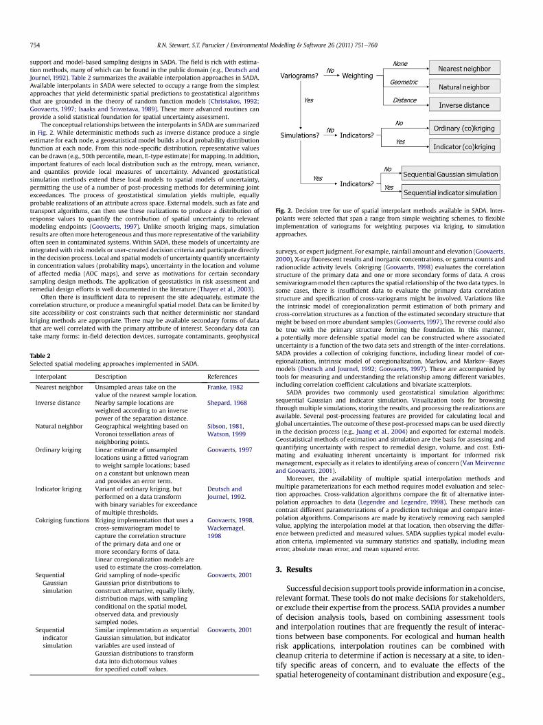
Fig. 2. Decision tree for use of spatial interpolant methods available in SADA. Inter-polants were selected that span a range from simple weighting schemes, to flexibleimplementation of variograms for weighting purposes via kriging, to simulationapproaches.

R.N. Stewart, S.T. Purucker / Environmental Modelling & Software 26 (2011) 751e760754

support and model-based sampling designs in SADA. The field is rich with estima-tion methods, many of which can be found in the public domain (e.g., Deutsch andJournel, 1992). Table 2 summarizes the available interpolation approaches in SADA.Available interpolants in SADA were selected to occupy a range from the simplestapproaches that yield deterministic spatial predictions to geostatistical algorithmsthat are grounded in the theory of random function models (Christakos, 1992;Goovaerts, 1997; Isaaks and Srivastava, 1989). These more advanced routines canprovide a solid statistical foundation for spatial uncertainty assessment.

The conceptual relationships between the interpolants in SADA are summarizedin Fig. 2. While deterministic methods such as inverse distance produce a singleestimate for each node, a geostatistical model builds a local probability distributionfunction at each node. From this node-specific distribution, representative valuescan be drawn (e.g., 50th percentile, mean, E-type estimate) for mapping. In addition,important features of each local distribution such as the entropy, mean, variance,and quantiles provide local measures of uncertainty. Advanced geostatisticalsimulation methods extend these local models to spatial models of uncertainty,permitting the use of a number of post-processing methods for determining jointexceedances. The process of geostatistical simulation yields multiple, equallyprobable realizations of an attribute across space. External models, such as fate andtransport algorithms, can then use these realizations to produce a distribution ofresponse values to quantify the contribution of spatial uncertainty to relevantmodeling endpoints (Goovaerts, 1997). Unlike smooth kriging maps, simulationresults are oftenmore heterogeneous and thusmore representative of the variabilityoften seen in contaminated systems. Within SADA, these models of uncertainty areintegrated with risk models or user-created decision criteria and participate directlyin the decision process. Local and spatial models of uncertainty quantify uncertaintyin concentration values (probability maps), uncertainty in the location and volumeof affected media (AOC maps), and serve as motivations for certain secondarysampling design methods. The application of geostatistics in risk assessment andremedial design efforts is well documented in the literature (Thayer et al., 2003).

Often there is insufficient data to represent the site adequately, estimate thecorrelation structure, or produce a meaningful spatial model. Data can be limited bysite accessibility or cost constraints such that neither deterministic nor standardkriging methods are appropriate. There may be available secondary forms of datathat are well correlated with the primary attribute of interest. Secondary data cantake many forms: in-field detection devices, surrogate contaminants, geophysical

Table 2Selected spatial modeling approaches implemented in SADA.

Interpolant Description References

Nearest neighbor Unsampled areas take on thevalue of the nearest sample location.

Franke, 1982

Inverse distance Nearby sample locations areweighted according to an inversepower of the separation distance.

Shepard, 1968

Natural neighbor Geographical weighting based onVoronoi tessellation areas ofneighboring points.

Sibson, 1981,Watson, 1999

Ordinary kriging Linear estimate of unsampledlocations using a fitted variogramto weight sample locations; basedon a constant but unknown meanand provides an error term.

Goovaerts, 1997

Indicator kriging Variant of ordinary kriging, butperformed on a data transformwith binary variables for exceedanceof multiple thresholds.

Deutsch andJournel, 1992.

Cokriging functions Kriging implementation that uses across-semivariogram model tocapture the correlation structureof the primary data and one ormore secondary forms of data.Linear coregionalization models areused to estimate the cross-correlation.

Goovaerts, 1998,Wackernagel,1998

SequentialGaussiansimulation

Grid sampling of node-specificGaussian prior distributions toconstruct alternative, equally likely,distribution maps, with samplingconditional on the spatial model,observed data, and previouslysampled nodes.

Goovaerts, 2001

Sequentialindicatorsimulation

Similar implementation as sequentialGaussian simulation, but indicatorvariables are used instead ofGaussian distributions to transformdata into dichotomous valuesfor specified cutoff values.

Goovaerts, 2001

surveys, or expert judgment. For example, rainfall amount and elevation (Goovaerts,2000), X-ray fluorescent results and inorganic concentrations, or gamma counts andradionuclide activity levels. Cokriging (Goovaerts, 1998) evaluates the correlationstructure of the primary data and one or more secondary forms of data. A crosssemivariogrammodel then captures the spatial relationship of the two data types. Insome cases, there is insufficient data to evaluate the primary data correlationstructure and specification of cross-variograms might be involved. Variations likethe intrinsic model of coregionalization permit estimation of both primary andcross-correlation structures as a function of the estimated secondary structure thatmight be based onmore abundant samples (Goovaerts, 1997). The reverse could alsobe true with the primary structure forming the foundation. In this manner,a potentially more defensible spatial model can be constructed where associateduncertainty is a function of the two data sets and strength of the inter-correlations.SADA provides a collection of cokriging functions, including linear model of cor-egionalization, intrinsic model of coregionalization, Markov, and MarkoveBayesmodels (Deutsch and Journel, 1992; Goovaerts, 1997). These are accompanied bytools for measuring and understanding the relationship among different variables,including correlation coefficient calculations and bivariate scatterplots.

SADA provides two commonly used geostatistical simulation algorithms:sequential Gaussian and indicator simulation. Visualization tools for browsingthroughmultiple simulations, storing the results, and processing the realizations areavailable. Several post-processing features are provided for calculating local andglobal uncertainties. The outcome of these post-processedmaps can be used directlyin the decision process (e.g., Juang et al., 2004) and exported for external models.Geostatistical methods of estimation and simulation are the basis for assessing andquantifying uncertainty with respect to remedial design, volume, and cost. Esti-mating and evaluating inherent uncertainty is important for informed riskmanagement, especially as it relates to identifying areas of concern (Van Meirvenneand Goovaerts, 2001).

Moreover, the availability of multiple spatial interpolation methods andmultiple parameterizations for each method requires model evaluation and selec-tion approaches. Cross-validation algorithms compare the fit of alternative inter-polation approaches to data (Legendre and Legendre, 1998). These methods cancontrast different parameterizations of a prediction technique and compare inter-polation algorithms. Comparisons are made by iteratively removing each sampledvalue, applying the interpolation model at that location, then observing the differ-ence between predicted and measured values. SADA supplies typical model evalu-ation criteria, implemented via summary statistics and spatially, including meanerror, absolute mean error, and mean squared error.

3. Results

Successful decision support tools provide information ina concise,relevant format. These tools do not make decisions for stakeholders,or exclude their expertise from the process. SADA provides a numberof decision analysis tools, based on combining assessment toolsand interpolation routines that are frequently the result of interac-tions between base components. For ecological and human healthrisk applications, interpolation routines can be combined withcleanup criteria to determine if action is necessary at a site, to iden-tify specific areas of concern, and to evaluate the effects of thespatial heterogeneity of contaminant distribution and exposure (e.g.,

Table 3Subset of available interview processes.

Setup my siteDevelop sample designPlot my dataDraw a data screen mapDraw a ratio mapModel spatial correlationInterpolate my dataDraw a variance mapDraw a probability mapDraw a contoured risk mapDraw an area of concern mapCalculate cost versus cleanupDraw a LISA mapPerform geostatistical simulationSmooth/reduce borehole data

R.N. Stewart, S.T. Purucker / Environmental Modelling & Software 26 (2011) 751e760 755

Barabás et al., 2001; Juang et al., 2001; Saito and Goovaerts, 2000;Purucker et al., 2007, 2010; Schipper et al., 2008). Applying theseassessment tools in this manner can not only reduce decision errors,but also improve estimates of risk outcomes and assist in efficientlydesigning the risk management decisions that are ultimatelyimplemented.

3.1. Scalable interfacing and decision support

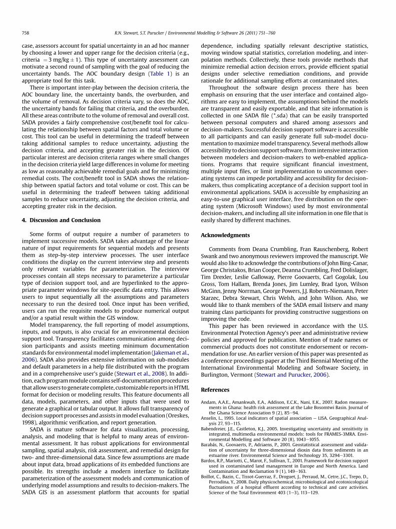
As the functionality of SADA grew with each successive version,so did the number of potential interactions between componentsand the risk for the software to become increasingly complicatedand hard to use. To address this, a highly scalable interface, referredto as the Interview-Steps-Parameters-Result (ISPR) approach, wasdeveloped. Themajority of the interface design space is divided intosteps, parameters, and results (Fig. 3). The ISPR provides a list of“interviews” that cover virtually every major function in everydaylanguage, summarized inTable 3. The interface components are thenorganized, parameterized, and displayed based on the specificinterview process chosen (Fig. 4). SADA uses the linear nature ofinputs required to implement sequential models and classifies themost common outputs, represented by environmental decisionsupport provided by the software, step-by-step. These interviewprocesses contain all steps necessary to parameterize a particulartype of decision support tool and are hyperlinked to the appropriateparameter windows for site-specific data entry. This allows users toinput sequentially assumptions andparameters necessary to run thedesired tool. Once inputhas beenverified, users can run the requisitemodels to produce numerical output and/or a spatial result withinthe GIS window. Because the step and parameter windows reorga-nize themselves for each situation, the interface “real-estate” is notfurther cluttered by additional interviews. Furthermore, users areguided through complicated assessments by well-organized steps.Anecdotally, this has proven particularly helpful for new users ofSADA and for educational applications.

Fig. 3. Conceptual diagram of the ISPR design. The ISPR provides a list of “interviews”that cover most major functions. The majority of the interface space is divided intosteps, parameters, and results. SADA uses the linear nature of inputs for thesesequential models and classifies the most common outputs, represented by environ-mental decision support provided by the software, step-by-step. These interviewprocesses contain all steps necessary to parameterize a particular type of decisionsupport tool and are hyperlinked to the appropriate parameter windows for site-specific data entry. This allows users to input sequentially assumptions and parametersnecessary to run the desired tool. Once input has been verified, users can run therequisite models to produce numerical output and/or a spatial result within the GISwindow. Because the step and parameter windows reorganize themselves for eachsituation, the interface “real-estate” is not further cluttered by additional interviews.

This organization of the interface (Fig. 5) facilitates modeldocumentation and transparency. Model transparency, the fullreporting of model assumptions, inputs, and outputs, is critical forfacilitating communication among decision participants and formeeting minimum documentation standards for environmentalmodel implementation (Jakeman et al., 2006). SADA providesextensive information on its sub-modules and default parameters ina help file distributed with the program and in a comprehensiveguide for users (Stewart et al., 2008). In addition, eachmodule of theprogram contains self-documentation procedures that allow usersto generate customizable HTML reports for modeling results. Thisfeature documents all data, models, parameters, and other inputsthat were used to generate any given graphical or tabular output; itallows full transparency of decision support processes and assists inmodel evaluation, algorithmic verification, and report generation.

3.2. Risk assessment

The strength of SADA’s particular implementation of spatialmodeling comes from direct integration with human health andecological risk models; together these contribute directly to deci-sion support. This is accomplished by using geostatistical methodsthat generate local distributions and calculating the probability thata threshold value is exceeded at each location on a prediction grid.This provides local models of spatial uncertainty based on a deci-sion threshold value. The threshold can be based on human healthrisk, ecological risk, regulatory criteria, or a customized valueprovided by users.

3.2.1. Human health riskHuman health risk assessment results are used to evaluate

concentration levels at a site to determine if risks are significant,whether remedial actions are needed, and to assist in determiningremedial cleanup levels. Typically, these assessments focus onchemicals, land use scenarios, exposure pathways that are expectedto occur at a site currently and under potential future conditions.The five land use scenarios considered in SADA include industrial,residential, recreational, excavation, and agricultural. Currentcontaminant concentrations are often used for the on-site assess-ment of future exposure; however, modeled results that representfuture contaminant concentrations can also be imported. In thesoftware, users select exposure pathways used to calculate totalrisk, and separate calculations are conducted for surface soil,sediment, groundwater, and surface water. SADA’s risk modelsfollow the U.S. Environmental Protection Agency (USEPA) guidance(1989 et seq.) and model input parameters can be modified to fitsite-specific exposure conditions.

The human health analysis tools support screening and fullbaseline risk assessments. An importantfirst step in both approaches

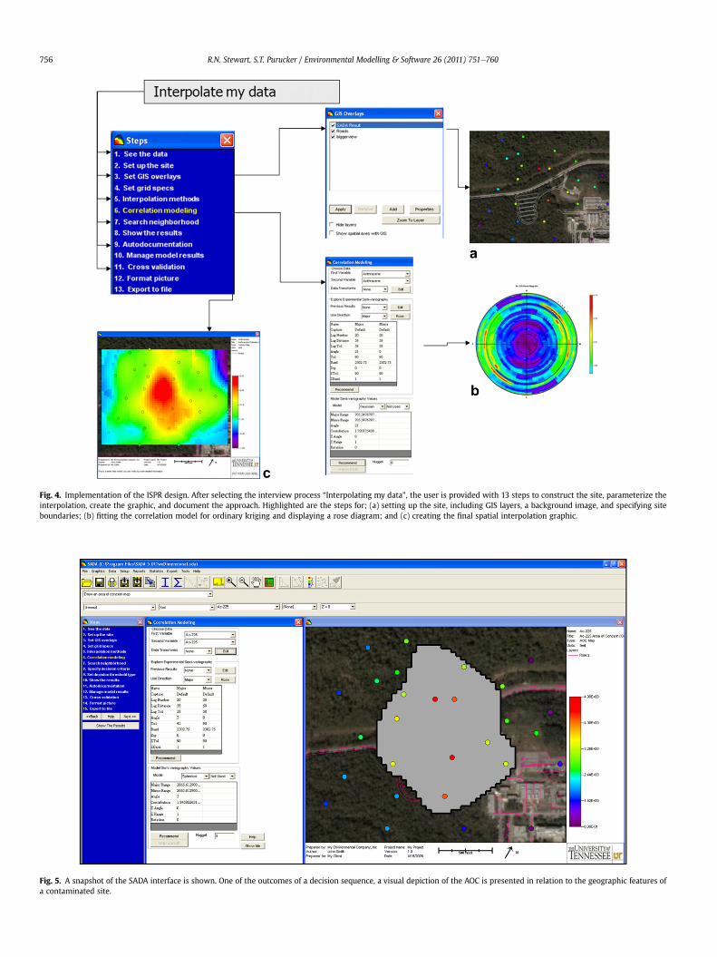
Fig. 4. Implementation of the ISPR design. After selecting the interview process “Interpolating my data”, the user is provided with 13 steps to construct the site, parameterize theinterpolation, create the graphic, and document the approach. Highlighted are the steps for; (a) setting up the site, including GIS layers, a background image, and specifying siteboundaries; (b) fitting the correlation model for ordinary kriging and displaying a rose diagram; and (c) creating the final spatial interpolation graphic.

Fig. 5. A snapshot of the SADA interface is shown. One of the outcomes of a decision sequence, a visual depiction of the AOC is presented in relation to the geographic features ofa contaminated site.

R.N. Stewart, S.T. Purucker / Environmental Modelling & Software 26 (2011) 751e760756

Fig. 6. Quantifying uncertainty in the AOC. The dark black line represents theboundary line for the current AOC. If no uncertainty were included in the analysis,everything inside this line would be part of the AOC. Conversely, everything outsidethis boundary would be considered clean. Application of the uncertainty bands showsthere are actually three areas. The first area, shown in black, continues to be designatedwithin the AOC even when uncertainty is considered. The dark gray area inside theboundary line is that portion of the AOC which may be improperly classified ascontaminated; there is a reasonable chance that this area could be excluded from theAOC if more data were available (false positive). The light gray area outside theboundary line indicates the space classified as clean that may, in fact, be contaminated(false negative) after accounting for spatial uncertainty.

R.N. Stewart, S.T. Purucker / Environmental Modelling & Software 26 (2011) 751e760 757

is the use of screening concentrations. A screening concentrationlimit can be back-calculatedwithin the software for a target risk levelor imported from an external file; these values then screen potentialcontaminants of concern. A lengthy list of detected contaminants ata site often can be reduced by such risk screening. SADA containsadditionaldata screensandstatistical tests that considerbackground,sample detection frequency, bioavailability, and whether detectedcontaminants are essential nutrients. Examples include univariatestatistics and specific functions such as non-parametric comparisontests (e.g., Wilcoxon Rank Sum test for comparing data tobackground).

Additional decision support output includes tables of forwardcalculations of exposure and risk used to support a full baseline riskassessment for the contaminants of concern. The exposureconcentrations are calculated based on statistical requirements ofthe data set, and scenario exposures and associated risks aregenerated. Detailed assessment of reasonable maximum exposureand central tendency exposure, cancer and non-cancer risks arethen calculated for multiple contaminants using site-specificinformation. SADA produces tables of output that can be modifiedto support risk assessment documentation purposes (U.S.Environmental Protection Agency (USEPA), 2001b). For identifiedcontaminants of concern, it also can provide spatial data screens tovisualize where exceedances are found and risk can be mappedusing the available interpolation functions.

3.2.2. Ecological riskEcological risk assessment encompasses a range of approaches to

estimate the probability and magnitude of effects on ecologicalendpoints (Suter, 2008). Ecological risk assessment is a multi-stepprocess that begins with screening and culminates in characteriza-tion of ecological risks from human activities (U.S. EnvironmentalProtection Agency (USEPA), 1993, 1998, 2003a). Although there arewell-established frameworks for performing these assessments,there are still many challenges and limitations that impact theirimplementation and usefulness (Kaputska, 2008), some of whichcan be addressed by freely available, competent decision supportsystems.

The ecological risk module allows benchmark screenings andgives users the ability to calculate forward dose for several terres-trial and aquatic receptors. Hazard identification consists ofcomparing (or screening) chemical-specific measurements toenvironmental effects concentrations derived from toxicity testingor other sources (benchmarks). Site contaminants that exceed thesebenchmarks are kept for further examination. SADA contains one ofthe most complete, publicly available compilations of benchmarksources and allows users to screen the data and site areas in a GISview or tabular form. Benchmarks also can be adjusted for site-specific physical parameters. Exposure assessment determines theecological receptors and pathways to model after consideringaccount bioavailability, behavior, growth, and spatial distributionsof contaminants and receptors. Exposure can also be measureddirectly via receptor body burdens or tissue residues. The softwareallows users to input toxicity reference values from the literature(e.g., California Department of Toxic Substance Control (CDTSC),2002; U.S. Environmental Protection Agency (USEPA), 2007) aspart of the dose response evaluation. SADA provides terrestrialexposure models to assist in modeling body burdens for over 20species commonly found in North America (Purucker et al., 2009a).Each of these species can be parameterized as male, female, orjuvenile (U.S. Environmental Protection Agency (USEPA), 1993,2003b). The risk characterization integrates outcomes of theprevious steps to estimate the likelihood that significant effects areoccurring, or will occur, and to describe the nature, magnitude, andextent of effects on the designated assessment endpoints. Estimated

and measured dose results can be displayed spatially or in tables tosupport selective remedial design or convention risk assessmentdocumentation.

3.3. Selective remedial design

A central piece of SADA’s toolbox is the process for delineating anAOC, one or more spatially identified site areas that are of interest inthe assessment. An AOC can be based on a number of contaminationscenarios, including plume definitions, source terms, and contami-nation footprints. An AOC necessarily will include a boundary and anassociated volume specification, both of whichmay include a degreeof uncertainty. Spatial models, therefore, occupy a central role indefining AOCs, as well as assessing uncertainty in their delineation.AnAOC is defined througha set of decisionparameters. These includedecision criteria, uncertainty constraints, and specific engineeringconsiderations (e.g., overburden calculations). Decision scale is alsoimportant in designating an AOC. In block scale, any estimated nodevalue that exceeds a decision value is included in the AOC. At the sitescale, the decision basis is applied only to the modeled site average;blocks are sorted frommost to least contaminated and remediation issimulated by progressively replacing the concentrations in thehighestestimatedblockswithapost-remediationconcentrationuntilthe site-wide average falls below the decision criterion.

A fully designated AOC includes the area, boundary line, anduncertainty bands around the boundary. In SADA, uncertaintybands include nodes on the prediction grid that may be improperlyclassified due to uncertainty in the spatial contaminant distribution(Fig. 6). This concept is also known as “thick lines” (Savelieva et al.,2005) and provides a spatial first order estimate on false positiveand false negative decision errors when classifying contamination.SADA has two methods for quantifying uncertainty in the AOC:percentile intervals and value intervals. Recall that geostatisticalmethods generate contours by selecting a value, typically a centraltendency statistic, from the probability distribution. Values otherthan the central tendency may also be used to create uncertaintybands. By choosing the 25th, 50th, and 75th percentiles uncertaintybands can be generated for an AOC. Value intervals provide anoption for non-statistical models such as inverse distance. In this

R.N. Stewart, S.T. Purucker / Environmental Modelling & Software 26 (2011) 751e760758

case, assessors account for spatial uncertainty in an ad hoc mannerby choosing a lower and upper range for the decision criteria (e.g.,criteria ¼ 3 mg/kg� 1). This type of uncertainty assessment canmotivate a second round of sampling with the goal of reducing theuncertainty bands. The AOC boundary design (Table 1) is anappropriate tool for this task.

There is important inter-play between the decision criteria, theAOC boundary line, the uncertainty bands, the overburden, andthe volume of removal. As decision criteria vary, so does the AOC,the uncertainty bands for failing that criteria, and the overburden.All these areas contribute to the volume of removal and overall cost.SADA provides a fairly comprehensive cost/benefit tool for calcu-lating the relationship between spatial factors and total volume orcost. This tool can be useful in determining the tradeoff betweentaking additional samples to reduce uncertainty, adjusting thedecision criteria, and accepting greater risk in the decision. Ofparticular interest are decision criteria ranges where small changesin the decision criteria yield large differences in volume for meetingas low as reasonably achievable remedial goals and for minimizingremedial costs. The cost/benefit tool in SADA shows the relation-ship between spatial factors and total volume or cost. This can beuseful in determining the tradeoff between taking additionalsamples to reduce uncertainty, adjusting the decision criteria, andaccepting greater risk in the decision.

4. Discussion and Conclusion

Some forms of output require a number of parameters toimplement successive models. SADA takes advantage of the linearnature of input requirements for sequential models and presentsthem as step-by-step interview processes. The user interfaceconditions the display on the current interview step and presentsonly relevant variables for parameterization. The interviewprocesses contain all steps necessary to parameterize a particulartype of decision support tool, and are hyperlinked to the appro-priate parameter windows for site-specific data entry. This allowsusers to input sequentially all the assumptions and parametersnecessary to run the desired tool. Once input has been verified,users can run the requisite models to produce numerical outputand/or a spatial result within the GIS window.

Model transparency, the full reporting of model assumptions,inputs, and outputs, is also crucial for an environmental decisionsupport tool. Transparency facilitates communication among deci-sion participants and assists meeting minimum documentationstandards for environmentalmodel implementation (Jakeman et al.,2006). SADA also provides extensive information on sub-modulesand default parameters in a help file distributed with the programand in a comprehensive user’s guide (Stewart et al., 2008). In addi-tion, eachprogrammodule contains self-documentationproceduresthat allowusers togeneratecomplete, customizable reports inHTMLformat for decision or modeling results. This feature documents alldata, models, parameters, and other inputs that were used togenerate a graphical or tabular output. It allows full transparency ofdecision support processes andassists inmodel evaluation (Oreskes,1998), algorithmic verification, and report generation.

SADA is mature software for data visualization, processing,analysis, and modeling that is helpful to many areas of environ-mental assessment. It has robust applications for environmentalsampling, spatial analysis, risk assessment, and remedial design fortwo- and three-dimensional data. Since few assumptions are madeabout input data, broad applications of its embedded functions arepossible. Its strengths include a modern interface to facilitateparameterization of the assessment models and communication ofunderlying model assumptions and results to decision-makers. TheSADA GIS is an assessment platform that accounts for spatial

dependence, including spatially relevant descriptive statistics,moving window spatial statistics, correlation modeling, and inter-polation methods. Collectively, these tools provide methods thatminimize remedial action decision errors, provide efficient spatialdesigns under selective remediation conditions, and providerationale for additional sampling efforts at contaminated sites.

Throughout the software design process there has beenemphasis on ensuring that the user interface and contained algo-rithms are easy to implement, the assumptions behind the modelsare transparent and easily exportable, and that site information iscollected in one SADA file (*.sda) that can be easily transportedbetween personal computers and shared among assessors anddecision-makers. Successful decision support software is accessibleto all participants and can easily generate full sub-model docu-mentation tomaximizemodel transparency. Severalmethods allowaccessibility todecision support software, fromintensive interactionbetween modelers and decision-makers to web-enabled applica-tions. Programs that require significant financial investment,multiple input files, or limit implementation to uncommon oper-ating systems can impede portability and accessibility for decision-makers, thus complicating acceptance of a decision support tool inenvironmental applications. SADA is accessible by emphasizing aneasy-to-use graphical user interface, free distribution on the oper-ating system (Microsoft Windows) used by most environmentaldecision-makers, and including all site information in onefile that iseasily shared by different machines.

Acknowledgments

Comments from Deana Crumbling, Fran Rauschenberg, RobertSwank and two anonymous reviewers improved themanuscript. Wewould also like to acknowledge the contributions of John Bing-Canar,George Christakos, Brian Cooper, Deanna Crumbling, Fred Dolislager,Tim Drexler, Leslie Galloway, Pierre Goovaerts, Carl Gogolak, LouGross, Tom Hallam, Brenda Jones, Jim Lumley, Brad Lyon, WilsonMcGinn, Jenny Norrman, George Powers, J.J. Roberts-Niemann, PeterStarzec, Debra Stewart, Chris Welsh, and John Wilson. Also, wewould like to thank members of the SADA email listserv and manytraining class participants for providing constructive suggestions onimproving the code.

This paper has been reviewed in accordance with the U.S.Environmental Protection Agency’s peer and administrative reviewpolicies and approved for publication. Mention of trade names orcommercial products does not constitute endorsement or recom-mendation for use. An earlier version of this paper was presented asa conference proceedings paper at the Third Biennial Meeting of theInternational Environmental Modeling and Software Society, inBurlington, Vermont (Stewart and Purucker, 2006).

References

Andam, A.A.E., Amankwah, E.A., Addison, E.C.K., Nani, E.K., 2007. Radon measure-ments in Ghana: health risk assessment at the Lake Bosomtwi Basin. Journal ofthe Ghana Science Association 9 (2), 85e94.

Anselin, L., 1995. Local indicators of spatial association e LISA. Geographical Anal-ysis 27, 93e115.

Babendreier, J.E., Castleton, K.J., 2005. Investigating uncertainty and sensitivity inintegrated, multimedia environmental models: tools for FRAMES-3MRA. Envi-ronmental Modelling and Software 20 (8), 1043e1055.

Barabás, N., Goovaerts, P., Adriaens, P., 2001. Geostatistical assessment and valida-tion of uncertainty for three-dimensional dioxin data from sediments in anestuarine river. Environmental Science and Technology 35, 3294e3301.

Bardos, R.P., Mariotti, C., Marot, F., Sullivan, T., 2001. Framework for decision supportused in contaminated land management in Europe and North America. LandContamination and Reclamation 9 (1), 149e163.

Boillot, C., Bazin, C., Tissot-Guerraz, F., Droguet, J., Perraud, M., Cetre, J.C., Trepo, D.,Perrodina, Y., 2008. Daily physicochemical, microbiological and ecotoxicologicalfluctuations of a hospital effluent according to technical and care activities.Science of the Total Environment 403 (1e3), 113e129.

R.N. Stewart, S.T. Purucker / Environmental Modelling & Software 26 (2011) 751e760 759

Brus, D.J., de Gruijter, J.J., 1997. Random sampling or geostatistical modelling?Choosing between design-based and model-based sampling strategies for soil(with Discussion). Geoderma 80, 1e44.

Butt, T.E., Davidson, H.A., Kehinde, A., Oduyemi, O.K., 2008a. Hazard assessment ofwaste disposal sites. Part 1: literature review. International Journal of RiskAssessment and Management 10 (1e2), 88e108.

Butt, T.E., Lockley, E., Oduyemi, K.O.K., 2008b. Risk assessment of landfill disposalsitesdstate of the art. Waste Management 28, 952e964.

California Department of Toxic Substance Control (CDTSC), 2002. U.S. EPA Region 9Biological Technical Assistance Group (BTAG) recommended toxicity referencevalues for mammals (revision date 11/21/2002). Available from: <http://www.dtsc.ca.gov/assessingrisk/upload/eco_btag-mammal-bird-trv-table.pdf>,(accessed 15.07.08).

Carlon, C., Pizzol, L., Critto, A., Marcomini, A., 2007. A spatial risk assessmentmethodology to support the remediation of contaminated land. EnvironmentInternational 34 (3), 397e411.

Christakos, G., 1992. Random Field Models in Earth Sciences. Academic Press, SanDiego, CA.

Christakos, G., Olea, R., 1992. Sampling design for spatially distributed hydrogeologicand environmental processes. Advances in Water Resources 15, 219e237.

Chung, M.K., Hu, R., Cheung, K.C., Wong, M.H., 2007. Pollutants in Hong Kong soils:polycyclic aromatic hydrocarbons. Chemosphere 67 (3), 464e473.

Crumbling, D.M., Griffith, J., Powell, D.M., 2003. Improving decision quality: makingthe case for adopting next-generation site characterization practices. Remedi-ation Spring 2003.

Crumbling, D.M., 2001. Using the TRIAD approach to improve the cost-effectivenessof hazardous waste site cleanups. U.S. Environmental Protection Agency; Officeof Solid Waste and Emergency Response; Washington, D.C. EPA 542-R-01e016.

Davidson, J.R., 1994. ELIPGRID-PC: A PC Program for Calculating Hot Spot Proba-bilities. ORNL-TM-12774. Oak Ridge National Laboratory, Oak Ridge, Tennessee.

Denzer, R., 2005.Generic integrationofenvironmentaldecision support systemsdstate-of-the-art. Environmental Modelling and Software 20, 1217e1223.

Deutsch, C., Journel, A., 1992. GSLIB: Geostatistical Software Library and User’sGuide. Oxford University Press, New York, NY.

Franke, R., 1982. Scattered data interpolation: tests of some methods. Mathematicsof Computation 38 (157), 181e200.

Franklin, R.B., Mills, A.L., 2003. Multi-scale spatial heterogeneity for microbialcommunity structure in an eastern Virginia agricultural field. FEMS Microbi-ology Ecology 44, 335e346.

Geary, R.C., 1954. The contiguity ratio and statistical mapping. The IncorporatedStatistician 5, 115e145.

Gilbert, R.O., 1987. Statistical Methods for Environmental Pollution Monitoring. VonNostrad Reinhold, New York.

Gogolak, C.V., Powers, G.E., Huffert, A.M., 1998. A Nonparametric Statistical Meth-odology for the Design and Analysis of Final Status Decommissioning Surveys.Office of Nuclear Regulatory Research; U.S. Nuclear Regulatory Commission,Washington, D.C.

Gogolak, C.V., 2001. Marssim Power 2000 software. Available from: <http://www.gogolak.org/>, (accessed 30.03.10).

Goovaerts, P., 2010. Geostatistical software. In: Fischer, M.M., Getis, A. (Eds.),Handbook of Applied Spatial Analysis: Software tools, Methods, and Applica-tions. Springer, Heidelberg.

Goovaerts, P., 2001. Geostatistical modelling of uncertainty in soil science. Geo-derma 103 (1e2), 3e26.

Goovaerts, P., 2000. Geostatistical approaches for incorporating elevation into thespatial interpolation of rainfall. Journal of Hydrology 228 (1e2), 113e129.

Goovaerts, P., 1998. Ordinary cokriging revisited. Mathematical Geology 30 (1),21e42.

Goovaerts, P., 1997. Geostatistics for Natural Resource Evaluation. Oxford UniversityPress, New York.

Holland, J., Bartell, S.M., Hallam, T.G., Purucker, S.T., Welsh, C.J.E., 2003. Role ofcomputational toolkits in environmental management. Chapter 6. In: Dale, V.H.(Ed.), Ecological Modeling for Resource Management. Springer-Verlag,New York.

Hornbruch, G., Schäfer, D., Dahmke, A., 2009. Case study to derive a critical numberof monitoring wells for plume characterization at different quality standards.Grundwasser 14 (2), 81e95.

Ifatimehin, O.O., Ogbe, A., 2008. Geostatistical approach to the control of typhoidfever in Anyigba. International Journal of Ecology and Environmental Dynamics4, 34e40.

Isaaks, E., Srivastava, R.M., 1989. An Introduction to Applied Geostatistics. OxfordUniversity Press, New York.

Jakeman, A.J., Letcher, R.A., Norton, J.P., 2006. Ten iterative steps in developmentand evaluation of environmental models. Environmental Modelling and Soft-ware 21, 602e614.

Juang, K.-W., Chen, Y.-S., Lee, D.-Y., 2004. Using sequential indicator simulation toassess the uncertainty of delineating heavy-metal contaminated soils. Envi-ronmental Pollution 127 (2), 229e238.

Juang, K.-W., Lee, D.-Y., Ellsworth, T.R., 2001. Using rank-order geostatistics forspatial interpolation of highly skewed data in a heavy-metal contaminated site.Journal of Environmental Quality 30, 894e903.

Kaputska, L., 2008. Limitations of the current practices used to perform ecologicalrisk assessments. Integrated Environmental Assessment and Management 4 (3),290e298.

Legendre, P., Legendre, L., 1998. Numerical Ecology. Elsevier, Amsterdam.

Linkov, I., Varghese, A., Jamil, S., Seager, T.P., Kiker, G., Bridges, T., 2004. Multi-criteria decision analysis: a framework for structuring remedial decisions atcontaminated sites. In: Linkov, I., Ramadan, A. (Eds.), Comparative RiskAssessment and Environmental Decision Making. Kluwer, pp. 15e54.

Matott, L.S., Babendreier, J.E., Purucker, S.T., 2009. Evaluating uncertainty in inte-grated environmental models: a review of concepts and tools. Water ResourcesResearch 45, W06421. doi:10.1029/2008WR007301.

Moran, P.A., 1950. Notes on continuous stochastic phenomena. Biometrika 37,17e37.

Norrman, J., Purucker, S.T., Stewart, R.N., Back, P.-E., Englelke F., 2008. Frameworkfor optimizing the evaluation of data from contaminated soil in Sweden. In:Proceedings of ConSoil 2008, 10th International Conference on SoileWaterSystems, Milan, Italy.

Puckett, G., Shaw, T.C., 2005. Triad case study: former small arms training range.Remediation Journal 16 (2), 121e130.

Purucker, S.T., Welsh, C.J.E., Stewart, R.N., Starzec, P., 2007. Use of habitat-contam-ination spatial correlation to determine when to perform a spatially explicitecological risk assessment. Ecological Modelling 204 (1e2), 180e192.

Purucker, S.T., Stewart, R.N., Welsh, C.J.E., 2009a. SADA: ecological risk based deci-sion support system for selective remediation. Chapter 11. In: Marcomini, A.,Suter, G.W., Critto, A. (Eds.), Decision Support Systems for Risk BasedManagement of Contaminated Sites. Springer, New York, NY, pp. 239e256.

Purucker, S.T., Golden, H.E., Laniak, G.F., Matott, L.S., McGarvey, D.J., Wolfe, K., 2009b.Free and open source GIS tools: role and relevance in the environmental assess-ment community. Chapter 18. In: Madden, M. (Ed.), Manual of GIS. AmericanSociety for Photogammetry and Remote Sensing, Bethesda, MD, pp. 293e310.

Purucker, S.T., Stewart, R.N., Wulff, J., 2010. A spatial decision support system forefficient environmental assessment and remediation. In: Madden, M., Allen, E.(Eds.), Landscape Analysis Using Spatial Tools. Springer-Verlag.

R Development Core Team, 2010. R: A Language And Environment for StatisticalComputing. R Foundation for Statistical Computing, Vienna, Austria, ISBN 3-900051-07-0.

Rizzoli, A.E., Davis, J.R., 1999. Integration and re-use of environmental models.Environmental Modelling and Software 14, 493e494.

Rügner, H., Finkel, M., Kaschl, A., Bittens, M., 2006. Application of monitored naturalattenuation in contaminated land managementda review and recommendedapproach for Europe. Environmental Science and Policy 9, 568e576.

Saito, H., Goovaerts, P., 2000. Geostatistical interpolation of positively skewed andcensored data in a dioxin-contaminated site. Environmental Science andTechnology 34, 4228e4235.

Sauer, A., Schanze, J., Walz, U., 2007. Development of a GIS-based risk assessmentmethodology for flood pollutants. In: Marx Gómez, J., Sonnenschein, M.,Müller, M., Welsch, H., Rautenstrauch, C. (Eds.), Information Technologies inEnvironmental Engineering. Springer, pp. 357e366.

Savelieva, E., Demyanov, V., Kanevski, M., Serre, M.L., Christakos, G., 2005. BME-based uncertainty assessment of the Chernobyl fallout. Geoderma 128 (3e4),312e324.

Schipper, A.M., Loos, M., Ragas, A.M.J., Lopes, J.P.C., Nolte, B.T., Wijnhoven, S.,Leuven, R.S.E.W., 2008. Modeling the influence of environmental heterogeneityon heavy metal exposure concentrations for terrestrial vertebrates in riverfloodplains. Environmental Toxicology and Chemistry 27 (4), 919e932.

Shepard, D., 1968. A two-dimensional interpolation function for irregularly spaceddata. In: Proceedings of the 1968 23rd ACM national conference, ACM.

Sibson, R., 1981. A brief description of natural neighbor interpolation. In: Barnett, V.(Ed.), Interpreting Multivariate Data (Ch. 2). John Wiley, Chichester, pp. 21e36.

Sinha, P., Lambert, M.B., Schew,W.A., 2007. Evaluation of a risk-based environmentalhot spot delineation algorithm. Journal of Hazardous Materials 149, 338e345.

Smart, K.A., Jackson, C.R., 2009. Fine scale patterns in microbial extracellularenzyme activity during leaf litter decomposition in a stream and its floodplain.Microbial Ecology 58 (3), 591e598.

Steiniger, S., Hay, G.J., 2009. Free and open source geographic information tools forlandscape ecology. Ecological Informatics 4 (4), 183e195.

Stewart, R.N., Purucker, S.T., 2006. SADA: a freeware decision support tool inte-grating GIS, sample design, spatial modeling, and risk assessment. In:Proceedings of the Third Biennial Meeting of the International EnvironmentalModelling and Software Society, Burlington, Vermont.

Stewart, R.N., et al., 2008. SADA Version 5 User’s Guide. University of Tennessee.http://www.tiem.utk.edu/wsada/index.shtml Available from:

Sunila, R, Laine, E., Kremonova, O., 2004. Fuzzy model and kriging for imprecise soilpolygon boundaries. Geoinformatics 2004. In: Proceedings of the 12th Inter-national Conference on Geoinformatics, Sweden.

Suter II, G.W., 2008. Ecological risk assessment in the United States EnvironmentalProtection Agency: a historical overview. Integrated Environmental Assessmentand Management 4 (3), 285e299.

Thayer, W.C., Griffith, D.A., Goodrum, P.E., Diamond, G.L., Hassett, J.M., 2003.Applications of geostatistics to risk assessment. Risk Analysis 23 (5), 945e960.

Thompson, M., 1999. Sampling: the uncertainty that dares not speak its name.Journal of Environmental Modeling 1, 19e21.

U.S. Environmental Protection Agency (USEPA), 2007. ECOTOX user guide: ECOTOXicol-ogy database system. Version 4.0. Available from:<http:/www.epa.gov/ecotox/>.

U.S. Environmental Protection Agency (USEPA), 2006. Data Quality Assessment:Statistical Methods for Data Practitioners. Office of Environmental Information,Washington, D.C. EPA QA/G-9S; EPA/240/B-06/003.

U.S. Environmental Protection Agency (USEPA), 2005a. Case Study: Use of a Deci-sion Support Tool: Using FIELDS and SADA to Develop Contour Maps of

R.N. Stewart, S.T. Purucker / Environmental Modelling & Software 26 (2011) 751e760760

Contaminant Concentrations and Estimate Removal Volumes for Cleanup of Soilat the Marino Brothers Scrapyard Site, Rochester Borough, Pennsylvania. Officeof Superfund Remediation and Technology Innovation; Brownfields and LandRevitalization Technology Support Center, Washington D.C.

U.S. Environmental Protection Agency (USEPA), 2005b. Case Study for the Use ofa Decision Support Tool: Using SCRIBE to Manage Data During a Triad Inves-tigation, Milltown Redevelopment Site, Milltown, New Jersey. Office of Super-fund Remediation and Technology Innovation; Brownfields and LandRevitalization Technology Support Center, Washington D.C.

U.S. Environmental Protection Agency (USEPA), 2003a. Generic ecological riskassessment endpoints (GEAEs) for ecological risk assessment. Risk AssessmentForum, Washington, D.C. EPA/630/P-02/004F.

U.S. Environmental Protection Agency (USEPA), 2003b. Guidance for DevelopingEcological Soil Screening Levels. Office of Solid Waste and Emergency Response,Washington, D.C. OSWER Directive 9285.7e55.

U.S. Environmental Protection Agency (USEPA), 2002. Guidance on Choosinga Sampling Design for Environmental Data Collection for Use in Developinga Quality Assurance Project Plan. Office of Environmental Information, Wash-ington, DC. EPA QA/G-5S.

U.S. Environmental Protection Agency (USEPA), 2001a. Resources for StrategicInvestigation and Monitoring. Office of Solid Waste and Emergency Response.EPA 542-F-01e030b.

U.S. Environmental Protection Agency (USEPA), 2001b. Volume I e Human HealthEvaluation Manual (Part D, Standardized Planning, Reporting and Review ofSuperfund Risk Assessments). Office of Emergency and Remedial Response,Washington, DC. Publication 9285.7e47.

U.S. Environmental Protection Agency (USEPA), 2000. Guidance on the data qualityobjectives process. QA/G-4.

U.S. Environmental Protection Agency (USEPA), 1998. Guidelines for ecological riskassessment. Washington DC, Risk Assessmnet Forum. EPA/630/R-95/005F.

U.S. Environmental Protection Agency (USEPA), 1993. Wildlife exposure factorshandbook, vol. I & II. Washington, DC. EPA/600/R-93/187.

U.S. Environmental Protection Agency (USEPA), 1989. Risk Assessment Guidance forSuperfund. Volume I, Human Health Evaluation Manual (Part A). Office ofEmergency and Remedial Response, Washington, DC. EPA/540/1e89/002.

Van Meirvenne, M., Goovaerts, P., 2001. Evaluating the probability of exceedinga site-specific soil cadmium contamination threshold. Geoderma 102, 75e100.

Wackernagel, H., 1998. Multivariate Geostatistics: An Introduction with Applica-tions. Springer-Verlag Inc., New York.

Watson, D., 1999. The natural neighbor series manuals and source codes. Computers& Geosciences 25 (4), 463e466.

Yfantis, E.A., Flatman, G.T., Behar, J.V., 1987. Efficiency of kriging estimation forsquare, triangular, and hexagonal grids. Mathematical Geology 19 (3),183e205.