an efficient local coupled cluster method for accurate
TRANSCRIPT
THE JOURNAL OF CHEMICAL PHYSICS 135, 144116 (2011)
An efficient local coupled cluster method for accurate thermochemistryof large systems
Hans-Joachim Werner1,a) and Martin Schütz2,b)
1Institut für Theoretische Chemie, Universität Stuttgart, Pfaffenwaldring 55,D-70569 Stuttgart, Germany2Institut für Physikalische und Theoretische Chemie, Universität Regensburg, Universitätsstr. 31,D-93040 Regensburg, Germany
(Received 12 July 2011; accepted 31 August 2011; published online 13 October 2011)
An efficient local coupled cluster method with single and double excitation operators and perturba-
tive treatment of triple excitations [DF-LCCSD(T)] is described. All required two-electron integrals
are evaluated using density fitting approximations. These have a negligible effect on the accuracy but
reduce the computational effort by 1–2 orders of magnitude, as compared to standard integral-direct
methods. Excitations are restricted to local subsets of non-orthogonal virtual orbitals (domain ap-
proximation). Depending on distance criteria, the correlated electron pairs are classified into strong,
close, weak, and very distant pairs. Only strong pairs, which typically account for more than 90% of
the correlation energy, are optimized in the LCCSD treatment. The remaining close and weak pairs
are approximated by LMP2 (local second-order Møller-Plesset perturbation theory); very distant
pairs are neglected. It is demonstrated that the accuracy of this scheme can be significantly improved
by including the close pair LMP2 amplitudes in the LCCSD equations, as well as in the perturbative
treatment of the triples excitations. Using this ansatz for the wavefunction, the evaluation and trans-
formation of the two-electron integrals scale cubically with molecular size. If local density fitting
approximations are activated, this is reduced to linear scaling. The LCCSD iterations scale quadrat-
ically, but linear scaling can be achieved by neglecting some terms involving contractions of single
excitations. The accuracy and efficiency of the method is systematically tested using various approx-
imations, and calculations for molecules with up to 90 atoms and 2636 basis functions are presented.
© 2011 American Institute of Physics. [doi:10.1063/1.3641642]
I. INTRODUCTION
The coupled cluster method with single and dou-
ble excitations and a perturbative treatment of triple ex-
citations [CCSD(T)] has become the “Gold Standard” in
quantum chemistry (this expression is attributed to T. H.
Dunning). Provided that the Hartree-Fock reference function
is a good zeroth-order approximation and large basis sets
are used, CCSD(T) usually yields energy differences, such
as reaction energies with chemical accuracy (1 kcal/mol or
better), and also many other molecular properties can be
accurately predicted. However, there are two bottlenecks that
restrict the applicability of the CCSD(T) method to very small
molecules: First, the computational increases with O(N 7),
where N is a measure of the molecular size or the number
of correlated electrons. This causes a “scaling wall” that can-
not be overcome even with massively parallel supercomput-
ers. Second, the convergence of the correlation energy with
respect to the basis set size is very slow, and very large basis
sets are needed to obtain accurate results. The latter problem
can be much alleviated by adding terms to the wavefunction
that depend explicitly on the inter-electronic distances r12 (so-
called F12-methods). This will be addressed in the companion
paper,1 in which the current work is extended to include such
terms.
a)Electronic mail: [email protected])Electronic mail: [email protected].
The scaling problem can be overcome by exploiting the
fact that electron correlation in insulators is a short-range
effect. If a local orbital basis is used, approximations that
exploit the short-range character can be introduced, as first
proposed and implemented by Pulay and Saebø,2–6 and later
generalized and extended in our groups.7–23 These methods
are based on two distinct approximations: first, excitations
from a given pair of localized molecular orbitals (LMOs) are
restricted to a subspace (domain) of non-orthogonal projected
atomic orbitals (PAOs), which are spatially close to the two
LMOs. Second, the pairs of LMOs can be classified according
to their distance. Strong pairs, for which the two orbitals are
very close, are treated at the highest level, e.g., LCCSD(T),
and more distant weak pairs at lower level, e.g., LMP2. Very
distant pairs can be neglected. This has made it possible to
achieve linear scaling of the computational cost with molec-
ular size for the whole range of closed-shell single reference
methods.9–13,16 Based on the techniques described in this pa-
per, also an open-shell DF-LUCCSD(T0) method has recently
been developed, which will be described in Refs. 24 and
25. Furthermore, another variant, denoted OSV-LCCSD (lo-
cal coupled-cluster with orbital specific virtual orbitals), has
recently been implemented into our program.26 This is based
on tensor factorizations of the MP2 amplitudes.27 There are
also many other methods that exploit the locality of electron
correlation,28–40 but a review of all these methods is beyond
the scope of the current article.
0021-9606/2011/135(14)/144116/15/$30.00 © 2011 American Institute of Physics135, 144116-1
Downloaded 12 Dec 2011 to 132.199.144.50. Redistribution subject to AIP license or copyright; see http://jcp.aip.org/about/rights_and_permissions
144116-2 H. Werner and M. Schütz J. Chem. Phys. 135, 144116 (2011)
Our first linear scaling LCCSD implementation9 was
based on a semi-direct scheme. The integrals in the
LMO/PAO basis involving at most three PAOs were gener-
ated once and stored on disk (for simplicity, we will in the
following denote the integral classes with 1–4 PAOs as 1-
external to 4-external integrals, respectively). However, the
contributions of the 4-external integrals were accounted for
in an integral-direct manner by transforming in each itera-
tion the pair amplitude matrices into the AO basis and con-
tracting them with the integrals computed on the fly. Linear
scaling was achieved by pre-screening techniques. Despite the
asymptotic linear scaling property, this approach had several
disadvantages: first, the 2-electron integrals in the AO basis
had to be computed in each iteration. Second, the transforma-
tion of the amplitude matrices from the pair specific PAO to
the full AO basis reduces the sparsity and, therefore, the con-
traction with the 2-electron integrals was expensive. Third,
the efficiency of the integral screening techniques, which rely
on the sparsity of certain test densities, depends sensitively on
the structure of the molecule and the basis set. For molecules
with a compact three-dimensional structure low-order scaling
was reached only for very large systems, in particular, if ba-
sis sets with diffuse functions are used. Thus, calculations for
realistic molecules with good basis sets were still extremely
expensive.
Somewhat later, this problem was alleviated by a semi-
direct implementation,13 in which also the 4-external integrals
were transformed into the PAO basis and stored on disk. The
number of transformed integrals scales linearly with molecu-
lar size, and the contraction with the amplitudes is then very
fast. The bottleneck of this implementation is the integral-
direct transformation, which is very expensive, in particular
when large and diffuse basis sets are used.
The evaluation and transformation of the two-electron
integrals can be very much accelerated by using density fit-
ting (DF) approximations. The DF approximations are widely
used in electronic structure theory. Originating from density
functional theory (DFT) (Refs. 41–43) their usage spreads to-
day from HF,44–46 MP2,14,47–50 CC2,20,51 MP2-F12,52–55 up to
CCSD.16,56 Furthermore, for correlated calculations of peri-
odic systems DF is indispensable for an efficient method.57,58
The overall scaling of the computational effort with respect to
system size is not affected by standard DF, but it significantly
reduces the prefactor. Furthermore, for some methods such as
MP2 it reduces the scaling with respect to the basis set size per
atom, NAO/Natoms, from quartic to cubic. This leads to enor-
mous savings in calculations with large basis sets. If density
fitting is used with localized orbitals, domains can also be in-
troduced for the auxiliary basis set (local fitting), and then lin-
ear scaling can be achieved. This was first shown for the cal-
culation of the exchange contribution in local MP2 (Ref. 14)
and later extended to other methods.15,16, 46, 59–61 The errors
caused by density fitting approximations are generally very
small and systematic, in particular for energy differences.
As a first step towards a fully density fitted DF-
LCCSD(T) implementation, a linear scaling DF algorithm to
evaluate the 4-external integrals in LCCSD was presented al-
ready in 2003.16 In the current work, this approach is ex-
tended to treat all integral classes by density fitting. It will be
shown that overall this speeds up LCCSD(T) calculations by
1–2 orders of magnitude, in particular, when large basis sets
are used. For simplicity, the prefix DF will be omitted in the
following.
A preliminary (unpublished) version of the current
method has been available in MOLPRO (Refs. 85 and 86)
since some time. In the current work we describe the method
in detail, including recent enhancements, such as accelerated
LCCSD convergence, improved local density fitting approx-
imations, improved accuracy of weak pair approximations,
and more efficient approximations for treating the 3-external
integrals. Furthermore, we propose MP2 corrections for the
domain and basis set incompleteness errors.
The paper is organized as follows: in Sec. II some basic
concepts of LCCSD theory will be reviewed. In Sec. III, the
density fitting algorithms for the transformation of the various
integral classes will be discussed. Finally, illustrative exam-
ples and timings will be presented in Sec. IV.
II. THEORY
The LCCSD equations have been presented in full detail
by Hampel and Werner.7 Further aspects that are important
for achieving linear scaling of the computational cost with
molecular size have been discussed in our previous work.9
However, the formulation used in these papers differs from
the present one in some details as explained below, and we
will therefore briefly review the method as currently used in
our program.
A. Local orbital spaces
In order to introduce local approximations as required
to achieve low-order scaling of the computational cost with
molecular size, local orbitals have to be used. Orthonormal
occupied localized orbitals (LMOs) can be obtained by stan-
dard localization schemes, such has Foster-Boys62 or Pipek-
Mezey localization.63 Alternatively, natural localized orbitals
(NLMOs) (Ref. 64) can be employed, which have been found
to be less dependent on the basis set.18 The virtual orbital
space is more difficult to localize by unitary transformations,
and, therefore, non-orthogonal virtual orbitals are often gen-
erated. In the present work, we use PAOs,2 but other choices
are possible as well: for example, Neese et al.37 have suc-
cessfully used pair natural orbitals (PNOs), and Yang et al.27
proposed to use orbital specific virtuals (OSVs), obtained by
tensor factorizations of MP2 amplitudes. The latter method
has recently been implemented into our program and will be
reported in Ref. 26. The PNO and OSV methods have the ad-
vantage that a smaller number of virtual orbitals is required
to represent the wavefunction, but since the total number of
pair- or orbital-specific orbitals is much larger than the num-
ber of PAOs, the integral transformations are more difficult.
Furthermore, it is not yet clear how to treat triple excitations
with these schemes. Very recently, Jasík et al. have proposed
a new method to generate a single set of orthonormal virtual
orbitals65 that are supposed to be better localized than PAOs,
Downloaded 12 Dec 2011 to 132.199.144.50. Redistribution subject to AIP license or copyright; see http://jcp.aip.org/about/rights_and_permissions
144116-3 Local coupled cluster J. Chem. Phys. 135, 144116 (2011)
but these orbitals have not yet been used in local coupled-
cluster methods.
In the following, the indices i, j, . . . refer to LMOs, r, s
refer to PAOs, a, b refer to canonical virtual orbitals (VMOs),
and p, q refer to any orbitals. The PAOs are defined as
�
�φPAOr
�
=
virt�
a
�
�φa
��
φa
�
�φAOr
�
=
virt�
a
�
�φa
�
Qar, (1)
where |φAOr � are atomic orbitals. These are projected onto the
virtual orbital space, such that the PAOs are orthogonal on
all LMOs, �φPAOr |φLMO
i � = 0 for all i, r . We assume that the
AOs and VMOs are expanded in a common orbital basis set
(OBS) {χµ} and represented by coefficient matrices CAOµr and
Cvµa , respectively. The matrix Qar that transforms from the
canonical virtual orbitals to the PAOs can then be written as
Q = Cv†SCAO, (2)
where Sµν = �χµ|χν� is the overlap matrix of the OBS. Thus,
the coefficient matrix of the PAOs is
P = CvQ = CvCv†SCAO. (3)
The choice of the AOs |φAOr � is, in principle, arbitrary. For
numerical reasons, it is recommended that the PAOs result-
ing from inner-shell core orbitals are eliminated from the be-
ginning, since their norm would be almost zero if the cor-
responding LMOs strongly overlap with the AOs. In order
to make the selection of core AOs unique, a good general
choice is to use for each atom the canonical Hartree-Fock
AOs, represented only by the basis functions of the corre-
sponding atom, so thatCAO is a block-diagonal matrix. In case
that correlation consistent or atomic natural orbital basis sets
are used, the contracted basis functions χµ automatically cor-
respond either to atomic core or valence orbitals or to corre-
lation functions and, therefore, one can in these cases simply
choose CAO to be the unit matrix. Optionally, one can normal-
ize the PAOs; then CAO becomes a diagonal matrix contain-
ing the normalization factors. Since we will only use correla-
tion consistent basis sets, CAO is assumed to be diagonal from
now on.
B. The local CCSD equations
For non-metallic systems, the PAOs are local by defini-
tion. This makes it possible to introduce domain approxima-
tions: the single excitations from a LMO φi are restricted to a
subset of PAOs φPAOr , r ∈ [i], which are spatially close to the
LMO φi . The subsets [i] are denoted as orbital domains. Cor-
respondingly, the double excitations from a pair of LMOs φi ,
φj are restricted to a pair domain [ij ], which is the union of
the orbital domains [i] and [j ]. The definition of the domains
will be further discussed in Sec. II C. Furthermore, pair ap-
proximations can be introduced, and only the amplitudes of
strong pairs are optimized in the LCCSD. The pair approxi-
mations will be discussed in more detail in Sec. II D.
Using these approximations, the LCCSD wavefunction
can be defined as
� = exp(T )|0� (4)
with the cluster operator,
T =�
i
�
r∈[i]
Eri t
ir +
1
2
�
ij∈Ps
�
r,s∈[ij ]
Eri E
sj T
ijrs . (5)
Here |0� is the closed-shell Hartree-Fock reference function,
Eri are spin-conserving one-particle excitation operators, and
t ir and Tijrs are the singles and doubles amplitudes, respec-
tively. The index ranges r ∈ [i] and r, s ∈ [ij ] are confined
to the corresponding domains. The list of orbital pairs ij in
the second summation is restricted to a subset Ps of strong
pairs (possibly also close pairs are included, cf. Sec. II D).
Since for a given pair ij the excitation operators Eri and Es
j
commute, the doubles amplitude must satisfy the symmetry
relation Tijrs = T
jisr . For convenience in later expressions, the
redundant contributions ij and ji (i �= j ) are both included in
the summations.
A compact and computationally convenient form of
LCCSD amplitude equations is obtained by multiplying the
Schrödinger equation from the left by e−T and projecting with
the contravariant configurations,66,67
�ri =
1
2Er
i |0�, (6)
�rsij =
1
6
�
2Eri E
sj + Es
i Erj
�
|0�. (7)
This yields the linked CC residuals
rir =�
�ri
�
�e−T H eT�
�0�
, (8)
Rijrs =
�
�rsij
�
�e−T H eT�
�0�
, (9)
which must vanish for the desired solution, i.e., rir = 0 for
r ∈ [i] and Rijrs = 0 for r, s ∈ [ij ] (note that the orbital do-
mains [i] equal the diagonal pair domains [ii] and, there-
fore, do not need a special treatment). The explicit form of
the residuals is most easily derived first in the canonical MO
basis and then transformed into the PAO basis. They differ
from the CCSD equations in the canonical virtual orbital basis
by multiplications with the PAO overlap matrix SPAO = Q†Q
in all places where an amplitude index is not matched by an
integral index. We note that the current formulation of the
LCCSD equations differs from the one given in Ref. 7, which
was based on the unlinked CC equations (cf. Appendix A).
The full equations as used in the current work are given in
Appendix B.
In each LCCSD iteration, the residuals are used to deter-
mine updates for the amplitudes. For this purpose, it is neces-
sary to transform them into a pair-specific orthonormal basis,
φija =
�
r∈[ij ]
φPAOr W ij
ra, (10)
where the transformation matrices Wijra are obtained by solv-
ing the Fock equations in the domain [ij ] as
Fij
PAOWij = S
ij
PAOWij�
ij (11)
with �ij
ab = δab�ija . Here, F
ij
PAO and Sij
PAO are the Fock and
overlap matrices in the PAO basis for the domain [ij ]. Since
Downloaded 12 Dec 2011 to 132.199.144.50. Redistribution subject to AIP license or copyright; see http://jcp.aip.org/about/rights_and_permissions

144116-4 H. Werner and M. Schütz J. Chem. Phys. 135, 144116 (2011)
the full set of PAOs is linearly dependent, it may happen that
the PAOs in a domain are (nearly) linearly dependent. Redun-
dant functions are eliminated at this stage by removing the
eigenvectors of Sij
PAO that correspond to zero or very small
eigenvalues (singular value decomposition; the default value
for the threshold is 1.d-7). Note that for this purpose Sij
PAO
is represented in the unnormalized PAO basis (obtained with
CAO = 1), so that contributions of PAOs with a small norm
are eliminated first.
In each LCCSD macroiteration, updates of the ampli-
tudes are obtained by solving the LMP2-like linear equations,
0 = ri + F�ti −�
k
fikS�tk, (12)
0 = Rij + F�TijS + S�TijF
−�
k
S�
fik�Tkj + �Tikfkj
�
S. (13)
Using Eqs. (10) and (11), these equations can be solved it-
eratively (microiterations) by transforming them to the pair-
specific orthogonal basis. In each microiteration, amplitude
updates are calculated as
�tia = −
r ia
�(ii)a − fii
, (14)
�Tij
ab = −R
ij
ab
�ija + �
ij
b − fii − fjj
, (15)
where fii are the diagonal elements of the Fock matrix in the
LMO basis and
ri =
ri −�
k �=i
fikS�tk
Wii , (16)
Rij
= Wij †
Rij −�
k �=i
fikS�TkjS −�
k �=j
S�TikSfkj
Wij .
(17)
The amplitude updates are then transformed back into the
PAO basis,
�tiPAO = �tiWii†, (18)
�Tij
PAO = Wij�TijWij †. (19)
Typically, two microiterations per macroiteration are suffi-
cient to improve and stabilize convergence. Convergence of
the macroriterations can be further improved using the DIIS
(direct inversion of the iterative subspace) procedure. Some-
times it is also useful to add constant shifts to the denomina-
tors in Eqs. (14) and (15).
The correlation energy is computed by using an approxi-
mate LCCSD Lagrangian, with the assumption that the multi-
pliers are equal to the (contravariant) amplitudes (which holds
exactly in the LMP2 case, where this expression corresponds
TABLE I. Comparison of CCSD and LCCSD convergence. The number of
iterations needed to converge the amplitudes to an accuracy of 10−6 is shown.
The convergence criterion is that the square norms of the singles and doubles
amplitude changes are both smaller than 10−12. The aug-cc-pVTZ basis set
was used.
Molecule Canonical Locala Localb
C2H2 11 11 10
C4H4 10 11 10
CO2 11 11 11
H2CO 12 13 11
H2O2 13 14 12
C2H5OH 12 13 11
HCONH2 13 14 13
HCOOH 13 13 12
HCOOCH3 13 13 12
aWithout microiterations.bUsing 2 microiterations per macroiteration.
to the Hylleraas functional),
E = 2�
i
�
r∈i
t ir�
f ir + rir
�
+�
ij∈Ps
�
rs∈[ij ]
Dijrs
�
Kijrs + Rij
rs
�
+�
ij∈Pw
�
r,s∈[ij ]
T ijrs K
ijrs (20)
with
f ir = �i|f |r�, (21)
Kijrs = (ir|js), (22)
representing the Fock matrix elements and two-electron inte-
grals in the LMO/PAO basis, and
Dijrs = T ij
rs + t ir tjs , ij ∈ Ps, (23)
the composite LCCSD strong pair amplitudes.102 The weak
pair amplitudes, Tijrs , ij ∈ Pw are taken from a preceding
LMP2 calculation. The tilde indicates contravariant quanti-
ties, i.e., Tijrs = 2T
ijrs − T
ijsr and D
ijrs = 2D
ijrs − D
ijsr . The sin-
gles and doubles residuals rir and Rijrs go to zero at conver-
gence. Their inclusion makes the energy expression approx-
imately quadratic in errors of the amplitudes t ir and Tijrs and
thus leads to faster convergence of the energy.
A comparison of the convergence of canonical and local
coupled cluster calculations is presented in Table I. In the lo-
cal case, calculations with and without the additional microi-
terations are compared. In the third column of the table, the
off-diagonal elements fik in Eqs. (16) and (17) are neglected,
i.e., just the initial microiteration is performed. This corre-
sponds to the usual update procedure in canonical calcula-
tions. In the last column, two microiterations per macroitera-
tion were performed. Even though the improvements by using
the microiterations are not dramatic, the number of iterations
is never larger than for the canonical method. The microiter-
ations also stabilize the convergence of the energy, and in no
case more than nine iterations were needed to obtain an accu-
racy of 1 µH for the LCCSD energy (in Table I more iterations
were performed to accurately converge the amplitudes).
Downloaded 12 Dec 2011 to 132.199.144.50. Redistribution subject to AIP license or copyright; see http://jcp.aip.org/about/rights_and_permissions
144116-5 Local coupled cluster J. Chem. Phys. 135, 144116 (2011)
C. Choice of orbital domains
In most previous applications of local correlation meth-
ods as outlined in Sec. II B, the orbital domains were de-
termined by a procedure originally proposed by Boughton
and Pulay (BP) (Ref. 68) (for details about domain specifi-
cation in our program, see also Refs. 7 and 17). It turned out,
however, that this choice is rather strongly basis set depen-
dent. More recently, Mata and Werner18 proposed an alterna-
tive domain selection method that is based on natural popu-
lation analysis69 (NPA) and much more stable with respect to
the basis set.18 On the other hand, due to the lack of a clear
localization criterion to be put into the Lagrangian the latter
have the disadvantage of not being compatible with analytic
energy gradient calculations.15,70
Both for the BP and NPA methods, the domains com-
prise all PAOs at a selected set of atoms and, therefore, an
orbital domain is equivalent to a subset of atoms assigned
to the LMO. The standard domains obtained by the BP or
NPA procedure can be augmented by adding the PAOs at the
next shell(s) of neighboring atoms. In this way, it is possi-
ble to approach the canonical result systematically. Typically,
98%–99% of the correlation energy of the corresponding
canonical method for a given basis is recovered with standard
domains; if the domains are extended by one shell of neigh-
boring atoms, about 99.8%–99.9% of the full correlation
energy is obtained.14,17 It should be noted, however, that
domain extensions strongly increase the computational cost
(for LCCSD(T), the computational resources such as CPU
time and disk space increase with L4, where L is a measure
of the average domain size per pair).
Finally we note that the domains may change as a func-
tion of the geometry.71–73 This can be avoided by freezing
the domains determined at some geometry, e.g., the equilib-
rium distance. In most cases, this has very little effect on the
results and guarantees microscopically smooth potentials. In
case where the electronic structure strongly changes as a func-
tion of the geometry, it may be necessary to merge the do-
mains obtained at different structures. This has been discussed
and demonstrated in detail in Ref. 73.
D. Pair approximations
The second type of approximations in local correlation
methods is to introduce a hierarchy of pair classes, which
are treated at different levels. In our program, we distinguish
strong, close, weak, distant, and very distant pairs. By default,
only the strong pairs are included in the LCCSD, i.e., the sum-
mations over ij are restricted as indicated in Eqs. (5) and (20).
The close, weak, and distant pair amplitudes are optimized at
the LMP2 level and kept fixed thereafter. For this purpose,
an initial LMP2 calculation is performed for all (except very
distant) pairs, and the pair energies for the close, weak, and
distant pairs are added to the LCCSD energy in Eq. (20). One
can also solve the LMP2 equations with fixed strong-pair am-
plitudes from the converged LCCSD, but we found that this
makes virtually no difference for the accuracy of the results.
Very distant pairs are completely neglected. The integrals
(ri|sj ) for distant pairs ij can optionally be evaluated by
multipole approximations,74,75 but this is mainly of interest
to reduce the computational effort in LMP2 calculations for
very large systems. For LCCSD, the multipole approximation
would not save much time and is not recommended. Thus,
in the current paper, there is no difference between weak and
distant pairs.
Close pairs were originally introduced as a pair class in-
termediate between strong (LCCSD) and weak (LMP2) to
specify restricted lists of triples for local (T) calculations10,11
(cf. Sec. II E). Furthermore, the close pair amplitudes, deter-
mined at the LMP2 level, are included in the triples calcu-
lation. Meanwhile they can also be included in the LCCSD
residuals (option KEEPCLS=1). The inclusion of the close
pair amplitudes in the LCCSD amplitude equations for the
strong pairs requires only a relatively small additional ef-
fort. In particular, it does not affect the contributions of the
4-external integrals. A strong increase in the number of 3-
external integrals required in the LCCSD part can be avoided
by neglecting the contributions that are quadratic in the am-
plitudes (cf. Appendix B). As will be shown in Ref. 1, the
inclusion of close-pair amplitudes is particularly important
in the DF-LCCSD(T)-F12 method, since the explicitly cor-
related terms remove most of the domain error and then the
errors caused by the pair approximations dominate.
The assignment of orbital pairs to the pair classes de-
pends on the distance Rij of the LMOs φi and φj . This is
defined as the minimum distance between any atom in the do-
main [i] and any atom in the domain [j ].7 Alternatively, one
can use the minimum number of bonds between these two sets
of atoms. The advantage of the latter method is that it is in-
dependent of the bond lengths and works for any molecule.
The disadvantage is that under certain circumstances atoms
which are separated by many bonds can be spatially close (an
example will be presented at the end of Sec. IV). This prob-
lem can be avoided by using distance criteria to determine
the distant and very distant pairs, and connectivity criteria for
the remaining pair classes. Furthermore, it is sometimes use-
ful to determine the pair lists at one geometry (along with
the domains) and then to keep them fixed at other geometries,
as already discussed for the domains in Sec. II C. For exam-
ple, this is important when bonds are elongated at transition
states.76, 77 This is also the preferred way to avoid basis set su-
perposition errors (BSSE) in local correlation calculations on
intermolecular complexes and clusters.7, 78, 79
Unless otherwise noted, we will use connectivity criteria
in the current paper, and these will be defined in Sec. IV.
E. Triple excitations
In order to compute the local perturbative triples correc-
tion (T),10,11 the triple excitations Eri E
sj E
tkT
ijkrst are restricted
to triples domains [ijk] = [i] ∪ [j ] ∪ [k]. Furthermore, the
list of orbital triples ijk is (by default) restricted such that the
related pairs ij , ik, kj are close or strong, and at least one of
them is strong. The strong and close pair amplitudes as well
as the singles amplitudes are included in the triples equations.
Since the Fock matrix is not diagonal in the local basis,
the zeroth-order Hamiltonian is not diagonal in the basis of
triply excited determinants, and the perturbative triples equa-
tions need in principle to be solved iteratively. Even though
Downloaded 12 Dec 2011 to 132.199.144.50. Redistribution subject to AIP license or copyright; see http://jcp.aip.org/about/rights_and_permissions

144116-6 H. Werner and M. Schütz J. Chem. Phys. 135, 144116 (2011)
this is possible,11 it is expensive and requires to store all
triples amplitudes. By neglecting couplings induced by off-
diagonal elements fij in the occupied-occupied block of the
Fock matrix the equations can be decoupled (T0 approxi-
mation). Alternatively, the fij couplings can be treated by
first-order perturbation theory, which also avoids storage of
the triples amplitudes,11 yet is considerably more expensive
than the T0 approximation. Since the T0 triples correction
can be computed very efficiently and in most cases provides
sufficient accuracy it has been used throughout in the present
work.
The computational effort scales strictly linear with
molecular size. Thus, in sharp contrast to canonical methods,
where calculation of the (T) correction is the main bottleneck,
the evaluation of the local (T0) corrections usually takes only
a comparable or even shorter time than the LCCSD. It should
be noted, however, that the relative effort for the triples quite
strongly increases if the close-pair class is extended.
F. Further approximations to achieve linear scaling
The domain approximation in combination with the re-
striction of the LCCSD treatment to strong pairs automat-
ically leads to linear scaling for most terms in the LCCSD
equations. This is due to the fact that the residuals Rijrs have
to be computed only for the domains r, s ∈ [ij ] and that the
occupied pair labels of the residuals and amplitude matrices
are restricted to strong (or close) pairs. However, there are
some terms, in particular those involving single excitations,
for which this alone is not sufficient to achieve linear scaling.
One also has to exploit that certain integrals decay quickly
with the distance between the orbitals involved. This leads
to the definition of integral lists and integral domains as dis-
cussed in detail in Ref. 9. These lists and domains can be de-
termined in advance on the basis of distance criteria, which
makes it possible to achieve linear scaling not only in the
computation of the residuals, but also in the integral trans-
formations. The errors introduced by these truncations only
amount to a few microhartree and are negligible. We note that
in the current work some additional approximations have been
introduced to the contributions of the 3-external integrals in
the pair-singles coupling terms (cf. Appendix B for details).
These strongly reduce the number of 3-external integrals to
be computed and stored.
The only term for which linear scaling is not easily
achieved9 involves the contraction,
[G(E)]rs =�
i
[2(rs|iu) − (ri|su)]t iu. (24)
This matrix is needed for all r, s since it contributes to all
pairs [cf. Eqs. (B21) and (B24) in Appendix B]. Calculat-
ing G(E) can entirely be avoided by using an approxima-
tion which is based on the observation that these terms can-
cel to large extent with the corresponding terms involving
1-external, instead of the 3-external integrals, i.e., with the
terms involving lkli in the βikSTkjS contribution to the resid-
uals Rij [cf. Eqs. (B21) and (B23) in Appendix B]. If these
contributions along with those of G(E) are neglected (option
SKIPGE=1), only a small error results.9 This error is much
smaller than errors caused by the domain approximation, and
it is also much smaller than the difference between full CCSD
and quadratic configuration interaction. In the latter method,
these terms are also absent. The effect of this approxima-
tion on the accuracy and efficiency will be demonstrated in
Sec. IV.
III. LOCAL DENSITY FITTING APPROXIMATIONS
A. 0-2 external integrals
The 2-external exchange integrals Kklrs = (rk|ls) (rs
∈ [kl]K) are computed using density fitting as described in de-
tail in Ref. 14. The all-internal and 1-external integrals can be
obtained in the same way with very little extra cost. Since for
LCCSD the operator lists kl and operator domains [kl]K are
much larger than in the LMP2 case,9 it is usually not useful to
enable local fitting – the crossover point to linear scaling oc-
curs quite late, and for medium size calculations the overhead
exceeds the savings. However, despite the fact that without
local fitting the algorithm scales in the asymptotic limit cubi-
cally (with a low prefactor), the CPU times for this part of the
transformation are quite short and have never been a bottle-
neck in the calculations.
The 2-external Coulomb integrals Jijrs = (rs|ij ) are first
computed in the AO basis as
(µν|ij ) = (µν|A)dAij , (25)
where dAij are the fitting coefficients obtained in the generation
of the 0-external integrals, i.e.,�
B
(A|B)dBij = (A|ij ). (26)
Here and in the following, A,B refer to fitting basis functions
χA, χB , and the 2-index and 3-index Coulomb integrals are
defined as
(A|B) =
�
χA(r1) r−112 χB(r2)dr1dr2, (27)
(µν|A) =
�
χµ(r1)χν(r1)r−112 χA(r2)dr1dr2. (28)
The fitting coefficients dAij are kept in memory. The outermost
loop runs over blocks of AOs, µ ≥ ν, and for each block the
three-index integrals are computed and contracted on the fly
with the fitting coefficients. In the final step the integrals are
transformed into the PAO basis. In the asymptotic limit, the
algorithm scales cubically with molecular size, but as for the
2-external exchange integrals the time is usually short as com-
pared to other parts of the calculation.
B. 3- and 4-external integrals
The 3-external integrals (rs|kt) occur in various terms
involving contractions with the singles amplitudes,
[J(Ekj )]rs = (rs|kt)tjt , (29)
[K(Ekj )]rs = (rk|st)tjt , (30)
Downloaded 12 Dec 2011 to 132.199.144.50. Redistribution subject to AIP license or copyright; see http://jcp.aip.org/about/rights_and_permissions

144116-7 Local coupled cluster J. Chem. Phys. 135, 144116 (2011)
and with doubles amplitudes,
[K(Dij )]rk = (rs|kt)Dijst , (31)
as well as in the expression of the perturbative triples cor-
rection (see Appendix B for the explicit LCCSD equations).
The range of indices r, s, t for each LMO k is independent of
the molecular size and can be determined in advance (3-ext
domains). Thus, in the asymptotic limit, the number of these
integrals scales linearly with molecular size. A detailed de-
scription of the definition of the 3-ext domains can be found
in Appendix B.
The 4-external integrals (rt |su), on the other hand, just
appear in the external exchange operators,
[K(Dij )]rs = (rt |su)Dijtu, r, s, t, u ∈ [ij ], (32)
which contribute only to the doubles residual for pair ij . Since
all four indices of (rt |su) always belong to the same domain,
this set of integrals is usually as compact as the 3-external
integral set, in spite of the additional virtual orbital index.
Obviously, since the number of correlated pairs ij scales lin-
early with molecular size, and the pair domains are indepen-
dent of the molecular size, also the number of 4-external in-
tegrals scales linearly. However, different pair domains may
overlap and, therefore, the calculation and storage of a dif-
ferent integral set for each domain [ij ] would be highly re-
dundant. A non-redundant set of 4-external integrals can be
determined by first setting up a non-redundant list of center
quadruples (RSTU ); this makes use of the fact that the do-
mains always include all PAOs at a given center. The calcula-
tion and contraction of the 4-external integrals are then driven
by this list.13 Quite similarly, the 3-external integral set is
driven by a quadruple (kRST ) consisting of one LMO index
k and three centers, specifying the minimum set of integrals
required for the computation of all the terms as mentioned
above.
As the 0-2 external integrals, the 3- and 4-external inte-
grals are generated by utilizing density fitting. For the sake
of simplicity, each of these three subsets is computed inde-
pendently. In principle, common intermediates such as the
transformed 3-index integrals (ri|A) and (rs|A) and the cor-
responding fitting coefficients could be computed only once
and reused, but this has not been implemented. The main rea-
son for this is that the domain sizes for the individual integral
subsets are different, and this would cause considerable com-
plications.
Since the individual orbital product distributions are lo-
cal (products of spatially local one-electron functions), local
fitting can be applied. In the following, we outline our algo-
rithm for the 4-external integrals, for which local fitting is
most useful. Local fitting for the 3-external integrals proceeds
along similar lines. However, since the 3-external domains are
quite extended, the savings are smaller than in the 4-external
case, and the crossover point to the standard non-local fitting
method occurs only for larger molecular sizes. An example
where local fitting indeed leads to substantial savings is given
in Sec. IV (Table IX).
Local fitting makes it necessary to use the robust three-
term fitting expression,14,16, 80–82
(rs|tu) ≈�
A∈[RS]
dArs(A|tu) +
�
B∈[T U ]
dBtu(B|rs)
−�
A∈[RS]
�
B∈[T U ]
dArs(A|B)dB
tu (33)
or the symmetric two-term term formula,16
(rs|tu) ≈1
2
�
A∈[RS]
dArs(A|tu) +
�
B∈[T U ]
dBtu(B|rs)
.
(34)
Here, A ∈ [RS] represents an auxiliary fitting function con-
fined to a fit domain [RS]. This domain is related to the charge
distributions of the orbital products φPAOr (r)φPAO
s (r), where r
and s denote functions located at the centers R and S, respec-
tively. Thus, the fitting domains are specific to center pairs. dArs
are the fitting coefficients obtained by solving for each center
pair RS,
�
B∈[RS]
(A|B)dBrs = (A|rs), ∀A ∈ [RS]. (35)
Since this implies that the indices A,B, r, s refer to func-
tions that are spatially close, the computational effort scales
linearly with molecular size. In the case that full fit domains
are used (non-local fitting), all terms in Eqs. (33) and (34) are
identical, yielding the usual one-term expression of density
fitting.
In Ref. 16, a first implementation of local fitting for the
4-external integrals was presented. There the individual fit do-
mains [RS] were comprising the fitting functions of the cen-
ters of all center quadruples (RSTU ) containing the center
pair (RS). Optionally, further centers could be added to these
core fit domains based on a distance criterion. Such an ap-
proach, however, can only efficiently work if the correlated
orbitals i and j are spatially close. This is because the pair
domains [ij ] are the union of the orbital domains [i] and [j ]
and, therefore, the size of the fitting domain would depend on
the number of orbitals j that form pairs with a given orbital i.
In the case of extended pair lists or domains, this scheme be-
comes inefficient and a more advanced algorithm is desirable.
In the present work, we adopt a procedure developed for den-
sity fitting in the context of periodic systems,57,58, 83, 84 where
local fitting is not only more efficient, but also mandatory due
to the infinite nature of the physical system. The importance
of a certain center X for the product charge distribution of
orbitals r, s is measured by the quantity,58
qXrs = (1 + τrs)
�
µ∈X
�
�
ν∈X
PµrSµνPνs
�2
, (36)
where Pµr are the PAO coefficients as defined in Eq. (3)
and τrs permutes the indices r and s. This “pseudo popula-
tion” then is condensed to individual groups of product dis-
tributions for each center pair RS (for product distributions
Downloaded 12 Dec 2011 to 132.199.144.50. Redistribution subject to AIP license or copyright; see http://jcp.aip.org/about/rights_and_permissions
144116-8 H. Werner and M. Schütz J. Chem. Phys. 135, 144116 (2011)
rs) as
qXRS =
�
r∈R
�
s∈S
qXrs . (37)
The quantities qXRS are finally normalized over the center
range X and sorted for each individual center pair (RS). Core
fit domains then are specified for RS by adding more and
more centers X from the sorted list, until a certain threshold
is reached. The core fit domains can optionally be augmented
by further centers according to either a distance or a topology
criterion. The set of three-index integrals (A|tu) required in
the assembly step of the 4-external integrals adheres to united
fit domains,
(tu|A), A ∈ [RS],∀(RS) ∈ (RSTU ). (38)
IV. SAMPLE CALCULATIONS
The method presented in Secs. I–III is available in the
MOLPRO package of ab initio programs85,86 and has already
been successfully applied in various applications.19,76, 77, 87–90
For example, barrier heights in various enzymes have been
computed in the framework of the hybrid quantum mechan-
ical and molecular mechanics (QM/MM) approach, and the
effect of domain and pair approximations on the results has
been systematically investigated.76,77, 90 Furthermore, the ac-
curacy of the local coupled cluster method (without den-
sity fitting) has been tested for reaction energies17 and other
molecular properties, such as dipole moments and dipole
polarizabilities.89 Especially noteworthy is the possibility to
correlate only certain regions of a molecule in the vicinity of
the reaction center.19 Then the computation time for the cor-
relation calculation becomes independent of the size of the
rest of the molecule. It has been shown in Ref. 19 that rela-
tively small regions are sufficient to obtain converged reaction
energies.
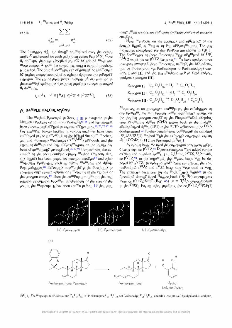
Here, we focus on the accuracy and efficiency of the
density fitting, as well as of pair approximations. The test
molecules considered for that purpose are shown in Fig. 1.
The geometries of these molecules were optimized by DF-
LMP2 using the cc-pVTZ basis set.91 We have studied three
reactions involving these molecules, namely, the hydrogena-
tion of progesteron via pregnenolon to pregnanediol (reac-
tions I and II), and the last synthetic step to yield andros-
tendione (reaction III),
Reaction I : C21O2H30 + H2 → C21O2H32.
Reaction II : C21O2H32 + 2H2 → C21O2H36.
Reaction III : C25O4H32 → C19O2H26 + C6O2H6.
Moreover, as an illustrative example for the capabilities of
our program, we will present some preliminary results on
the thermal reaction energy of the photodamaged cyclobu-
tane pyrimidine dimer (CPD) lesion back to the undam-
aged/repaired dimer (TpT) in the ATTA sequence of the DNA
double strand.92 Further benchmarks, comparing the standard
DF-LCCSD(T) method with the explicitly correlated variant
DF-LCCSD(T)-F12 are presented in Ref. 1.
As orbital basis we used the correlation consistent triple-
ζ basis sets, cc-pVTZ.93 Diffuse functions were added for the
oxygen and nitrogen atoms, i.e., C,H=cc-pVTZ, O,N=aug-
cc-pVTZ.94 In the following, this mixed basis will be de-
noted by aVTZ. In order to study basis set effects, the cor-
responding aVQZ and aV5Z basis sets were used as well.
The auxiliary basis sets for the Fock-matrix fitting46 in the
preceding density fitted Hartree-Fock (DF-HF) calculations
were cc-pVnZ/JKFIT (Ref. 45) (n = T,Q,5 corresponding
to the OBS). For all other integrals, the cc-pVTZ/MP2FIT,
(a) Progesteron (b) Pregnenolon (c) Pregnanediol
(d)
O
H
H H
O
O
O
O
OO
H H
H
O
+
H
H
Androstendione Precursor Androstendione Ortho-
hydroxyphenol
FIG. 1. The molecules (a) progesterone C21O2H30, (b) pregnenolone C21O2H32, (c) pregnanediol C21O2H36, and (d) a reaction step yielding androstendione.
Downloaded 12 Dec 2011 to 132.199.144.50. Redistribution subject to AIP license or copyright; see http://jcp.aip.org/about/rights_and_permissions

144116-9 Local coupled cluster J. Chem. Phys. 135, 144116 (2011)
TABLE II. Definition of pair classes based on connectivity criteria. Here,
n is the number of bonds between the orbital domains [i] and [j ] that form
a pair ij . The input parameters IVDIST, IWEAK, ICLOSE, and KEEPCLS
are abbreviated as v, w, c, and k, respectively. In the current work, there is no
difference between weak and distant pairs. Unless otherwise noted the default
IVDIST = 8 was used.
Pair class Criteria Amplitudes
Strong n < c Optimized by LCCSD
Closea c ≤ n < w Optimized by LMP2
but included in LCCSD(T0)
Weak w ≤ n < v Optimized by LMP2,
neglected in LCCSD(T0)
Very distant v ≤ n Entirely neglected
aIf k = 0, these pairs are neglected in the LCCSD residuals but included in the (T0) cal-
culation. If k = 1, they also contribute to the strong pair and singles LCCSD residuals.
cc-pVQZ/MP2FIT, or cc-pV5Z/MP2FIT (Ref. 50) basis sets
have been used; as for the OBS, the corresponding augmented
basis sets were used for the oxygen and nitrogen atoms. Nat-
ural localized molecular orbitals were employed, and unless
otherwise noted the NPA with the threshold NPASEL=0.07
was used to determine the domains as described in Ref. 18.
Option MERGEDOM=1 was used, which merges overlapping
domains of the π -orbitals in aromatic rings of reaction III,
yielding identical domains that extend over all six atoms (for
all other reactions studied in this paper there is no effect). Lo-
cal fitting was used only when indicated.
As outlined in Sec. II D, the definition of the pair classes
is based on the number of bonds (n) between the closest
atoms of the two orbital domains of a pair. In the current
benchmarks, the numbers of strong, close, and weak pairs are
varied. The parameters IWEAK and ICLOSE affect the as-
signment of the pairs to these three classes. The additional
parameter KEEPCLS affects the approximations made for the
different pair classes. The meaning of the three parameters is
summarized in Table II. In the following, we will use the ab-
breviation wck, so that, e.g., wck = 321 means IWEAK=3,
ICLOSE=2, KEEPCLS=1. In addition, we will test the ef-
fect of neglecting G(E) along with the corresponding con-
tributions of the one-external integrals (option SKIPGE=1,
cf. Sec. II F).
We will first test the errors caused by the density fit-
ting approximation. Table III shows the errors of the DF-
TABLE III. Fitting errors � and additional local fitting errors δsymm (us-
ing symmetric formula, Eq. (34)), δrobust (using robust formula, Eq. (33))
for pregnanediole, DF-LCCSD/aVTZ. All values are given in µEh. For the
LCCSD method, the errors refer to the total correlation energy (including the
weak pair LMP2 contributions) for (T0) to the triples contribution only.
0-3 ext. aVTZ aVTZ aVQZ aVQZ aV5Z
4-ext. aVTZ aVQZ aVQZ aV5Z aV5Z
� (LMP2) 458 458 157 157 5
� (LCCSD) −1976 147 −100 103 −22
δsymm(LCCSD) −150 −43 −39 −12 −10
δrobust(LCCSD) −151 −42 −39 −10 −9
�(T0) −78 −71 −3 −3 −1
δsymm(T0) −22 −20 0 0 1
δrobust(T0) −8 −5 0 0 0
TABLE IV. Effect of density fitting approximations on reaction energies (in
kJ mol−1). wck = 210, SKIPGE = 0. Basis: aVTZ.
Fitting basis HF LCCSD LCCSD(T0)
0-3 ext. 4-ext. I II I II I II
Integral-direct −59.2 −195.0 −75.0 −218.6 −70.9 −209.4
aVTZ aVTZ −59.3 −195.1 −75.2 −218.7 −71.1 −209.5
aVTZ aVQZ −59.3 −195.1 −75.2 −218.8 −71.1 −209.6
LCCSD correlation energy of pregnanediol as compared to
an integral-direct LCCSD calculation without density fitting.
For comparison, the errors of the corresponding DF-LMP2
calculations are also presented. It is found that fitting the 0-3
external integrals in the DF-LCCSD does not lead to an error
that is significantly larger than for DF-LMP2, even though the
fitting basis set was optimized for MP2 and not for LCCSD.
However, the fitting approximation is more critical for the 4-
external integrals, since these involve more virtual orbitals
with a complicated node structure. This leads to an error that
is 4-5 times larger (and of opposite sign) than the fitting er-
ror in DF-LMP2. The error of the correlation energy is re-
duced by one order of magnitude if for the 4-external the
larger aVQZ/MP2FIT basis is used. It is then actually smaller
than the DF-LMP2 error, but this is certainly due to some er-
ror compensations between the different integral classes. The
errors due to local fitting are one order of magnitude smaller
than the fitting errors and thus negligible.
Table IV demonstrates the effect of the density fitting on
reaction energies. The Hartree-Fock values are affected by
0.1 kJ mol−1, the LCCSD, and LCCSD(T0) correlation con-
tributions by about the same amount. These errors are cer-
tainly negligible, even if only the aVTZ fitting basis is used
for the 4-external integrals. In all subsequent calculations, the
aVTZ/MP2FIT fitting basis set thus is used for all integral
classes.
The savings due to the density fitting approximations are
enormous. For pregnanediol, the standard integral-direct cal-
culation of the transformed integrals [using the programs de-
scribed in (Refs. 9 and 95)] is about 50 times slower than with
the current density fitting implementation. This ratio would
further increase if larger basis sets were used.
TABLE V. CPU times (in min on Intel W5590 @ 3.33 GHZ) for density
fitting integral transformations for pregnanediol. Basis set: aVTZ.
Integral set wck locfit=0 locfit=1
0-2-external 210 20.9 32.7
311 43.8 47.0
321 44.7 47.5
3-external 210 53.3 33.6
311 76.1 50.3
321 113.7 81.1
4-external 210 46.6 23.7
311 38.1 19.2
321 77.7 48.1
Downloaded 12 Dec 2011 to 132.199.144.50. Redistribution subject to AIP license or copyright; see http://jcp.aip.org/about/rights_and_permissions
144116-10 H. Werner and M. Schütz J. Chem. Phys. 135, 144116 (2011)
TABLE VI. Canonical DF-HF and DF-MP2 results for reaction energies
(see text).
DF-HF DF-MP2
BASIS I II III I II III
aVTZ −59.3 −195.1 −2.7 −73.2 −220.6 28.3
aVQZ −58.6 −192.9 −5.1 −74.5 −220.4 22.3
aV5Z −58.6 −192.7 −5.8 −74.7 −219.7 20.5
CBS[45] −58.6 −192.6 −5.9 −74.9 −219.4 19.2
Table V shows the CPU times to generate the transformed
integrals for pregnanediol with and without local density fit-
ting. As already mentioned, there is no saving for the 0-2 ex-
ternal integrals – in contrary, the overhead for local fitting in-
creases the CPU times. Therefore, local fitting is not recom-
mended for this class of integrals. However, there are signif-
icant savings for the 3-external and 4-external integrals. The
time to generate the latter is almost reduced by a factor of 2.
Naturally, the savings get somewhat smaller if the pair lists
are extended, since then the linear scaling regime is reached
later.
Next we will assess the domain errors and basis set ef-
fects on the reaction energies. Normally, canonical DF-MP2
calculations are easily possible for molecules that can be
treated by DF-LCCSD(T0). This makes it possible to esti-
mate the domain error by comparison of DF-LMP2 and DF-
MP2 calculations. Experience for smaller molecules, where
canonical coupled cluster calculations are still possible, has
shown that the domain errors are very similar at the LMP2
and LCCSD levels, and thus it is possible to add a correction
�EMP2 = EMP2 − ELMP2 to the LCCSD(T0) results. If DF-
MP2 results are available for larger basis sets, this may also
include a basis set correction. The DF-MP2 reaction energies
for aVTZ, aVQZ, and aV5Z, as well as the extrapolated basis
set limits are presented in Table VI. The latter have been ob-
tained by Karton-Martin extrapolation96 of the Hartree-Fock
values and by n−3 extrapolation97 of the correlation energies.
The corresponding DF-LMP2/aVTZ values for reactions I–
III are −69.2, −211.5, and 15.3 kJ mol−1, respectively, yield-
ing domain corrections of −4.0, −9.1, and +13.0 kJ mol−1,
respectively. The additional basis set corrections are −1.7,
+1.2, and −9.1 kJ mol−1, yielding total corrections of −5.7,
−7.9, and +3.9 kJ mol−1.
In particular for reaction III the domain error of
13 kJ mol−1 is quite large. It can be observed, however,
that it has opposite sign as the basis set error, and actually
the LMP2/aVTZ value is in much better agreement with the
MP2/CBS value than with the MP2/aVTZ one. We believe
that this is due to strong BSSE effects in the canonical cal-
culation. It is well known that BSSE effects on the correla-
tion energies are strongly reduced by the local ansatz.7, 78, 79
In molecular clusters, this is due to the fact that double ex-
citations from one monomer to the other are excluded by the
local ansatz. Similarly, the absence of double excitations from
one part of the molecule to another can reduce intramolec-
ular BSSE effects, though this is more difficult to quantify.
In the current case, BSSE effects should favor the energy
of the large precursor relative to the products, making the
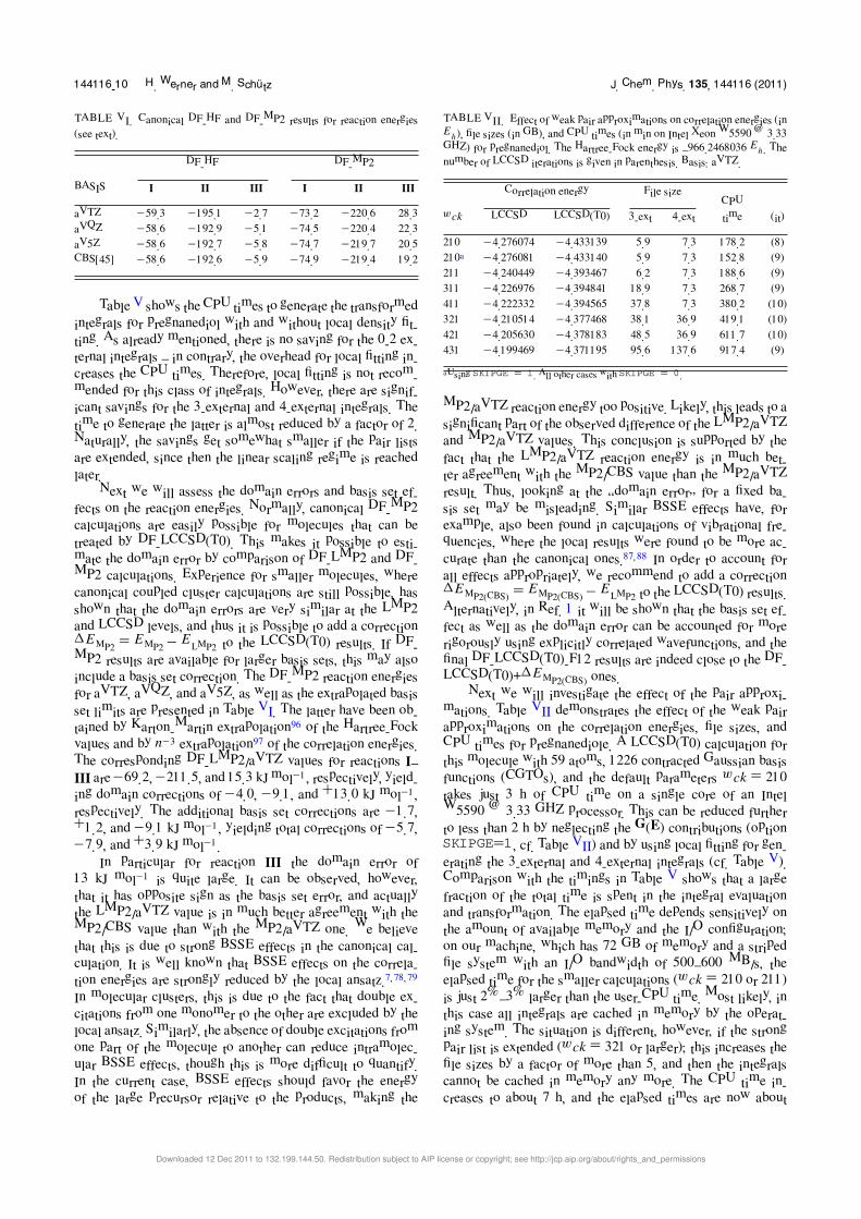
TABLE VII. Effect of weak pair approximations on correlation energies (in
Eh), file sizes (in GB), and CPU times (in min on Intel Xeon W5590 @ 3.33
GHZ) for pregnanediol. The Hartree-Fock energy is –966.2468036 Eh. The
number of LCCSD iterations is given in parenthesis. Basis: aVTZ.
Correlation energy File size
wck LCCSD LCCSD(T0) 3-ext 4-ext
CPU
time (it)
210 −4.276074 −4.433139 5.9 7.3 178.2 (8)
210a −4.276081 −4.433140 5.9 7.3 152.8 (9)
211 −4.240449 −4.393467 6.2 7.3 188.6 (9)
311 −4.226976 −4.394841 18.9 7.3 268.7 (9)
411 −4.222332 −4.394565 37.8 7.3 380.2 (10)
321 −4.210514 −4.377468 38.1 36.9 419.1 (10)
421 −4.205630 −4.378183 48.5 36.9 611.7 (10)
431 −4.199469 −4.371195 95.6 137.6 917.4 (9)
aUsing SKIPGE = 1. All other cases with SKIPGE = 0.
MP2/aVTZ reaction energy too positive. Likely, this leads to a
significant part of the observed difference of the LMP2/aVTZ
and MP2/aVTZ values. This conclusion is supported by the
fact that the LMP2/aVTZ reaction energy is in much bet-
ter agreement with the MP2/CBS value than the MP2/aVTZ
result. Thus, looking at the “domain error” for a fixed ba-
sis set may be misleading. Similar BSSE effects have, for
example, also been found in calculations of vibrational fre-
quencies, where the local results were found to be more ac-
curate than the canonical ones.87,88 In order to account for
all effects appropriately, we recommend to add a correction
�EMP2(CBS) = EMP2(CBS) − ELMP2 to the LCCSD(T0) results.
Alternatively, in Ref. 1 it will be shown that the basis set ef-
fect as well as the domain error can be accounted for more
rigorously using explicitly correlated wavefunctions, and the
final DF-LCCSD(T0)-F12 results are indeed close to the DF-
LCCSD(T0)+�EMP2(CBS) ones.
Next we will investigate the effect of the pair approxi-
mations. Table VII demonstrates the effect of the weak pair
approximations on the correlation energies, file sizes, and
CPU times for pregnanediole. A LCCSD(T0) calculation for
this molecule with 59 atoms, 1226 contracted Gaussian basis
functions (CGTOs), and the default parameters wck = 210
takes just 3 h of CPU time on a single core of an Intel
W5590 @ 3.33 GHZ processor. This can be reduced further
to less than 2 h by neglecting the G(E) contributions (option
SKIPGE=1, cf. Table VII) and by using local fitting for gen-
erating the 3-external and 4-external integrals (cf. Table V).
Comparison with the timings in Table V shows that a large
fraction of the total time is spent in the integral evaluation
and transformation. The elapsed time depends sensitively on
the amount of available memory and the I/O configuration;
on our machine, which has 72 GB of memory and a striped
file system with an I/O bandwidth of 500–600 MB/s, the
elapsed time for the smaller calculations (wck = 210 or 211)
is just 2%–3% larger than the user-CPU time. Most likely, in
this case all integrals are cached in memory by the operat-
ing system. The situation is different, however, if the strong
pair list is extended (wck = 321 or larger); this increases the
file sizes by a factor of more than 5, and then the integrals
cannot be cached in memory any more. The CPU time in-
creases to about 7 h, and the elapsed times are now about
Downloaded 12 Dec 2011 to 132.199.144.50. Redistribution subject to AIP license or copyright; see http://jcp.aip.org/about/rights_and_permissions

144116-11 Local coupled cluster J. Chem. Phys. 135, 144116 (2011)
TABLE VIII. Effect of weak pair approximationson LCCSD(T0) reaction
energies (in kJ mol−1). Basis: aVTZ.
LCCSD LCCSD(T0)
wck I II III I II III
210 −75.0 −218.5 22.2 −70.9 −209.4 15.2
210a −74.5 −218.0 22.0 −70.2 −208.6 15.0
211 −74.9 −219.2 23.3 −71.3 −211.0 16.8
311 −75.6 −219.1 21.4 −70.1 −209.0 17.7
411 −75.5 −218.6 18.8 −69.9 −208.6 16.9
321 −74.1 −218.6 20.8 −68.3 −208.6 17.7
421 −73.9 −217.8 18.0 −68.1 −207.9 17.0
431 −74.4 −218.3 17.3 −68.7 −208.6 16.3
aUsing SKIPGE = 1. All other cases with SKIPGE = 0.
20% larger than the CPU time. This is due to the fact that
in the LCCSD iterations the processing of the 3-external and
4-external integrals is strongly I/O bound. It can be seen in
Table VII that the correlation energies are reduced by includ-
ing more pairs in the LCCSD residual. This is not due to an
overestimation of the weak pair LMP2 energies, but due to
the additional strong and weak pair couplings in the LCCSD.
These couplings are approximately accounted for with option
KEEPCLS=1, which means that the close-pair LMP2 am-
plitudes are included in the LCCSD residuals for the strong
pairs. The standard choice of wck = 210 yields for pregnane-
diol a correlation energy that is about 1.4% larger than the
best current value, obtained with wck = 431. This error is re-
duced to 0.5% by using wck = 211, i.e., KEEPCLS=1, and
to 0.1% with wck = 321.
The LCCSD and LCCSD(T0) reaction energies are pre-
sented in Table VIII. The effect of SKIPGE=1 on the reaction
energies is small (0.2–0.8 kJ mol−1 in the current examples).
For reactions I and II, the LCCSD results are only weakly
affected by the pair approximations. The variations depend-
ing on the choice of the wck parameter amount only to about
1 kJ mol−1. This is probably due to the fact that in these cases
only OH-bonds are formed and no additional long-range cor-
relations occur. For LCCSD(T0), the effect of the weak pair
approximations on reactions I and II is somewhat larger than
for LCCSD; overall, extending the strong pair list reduces
the correlation effect on the reaction energies and, therefore,
makes the reactions less exothermic. In this case, however,
the choice wck = 211 yields somewhat worse agreement with
the best values for the reaction energies, and only extending
IWEAK to 3 improves the result. Apparently, different effects
of opposite sign partly compensate each other.
For reaction III, the situation is different. Extension of
the strong and/or close pair lists reduces the LCCSD re-
action energy by about 5 kJ mol−1. Likely, this is due to
the additional long-range correlation in the precursor rela-
tive to the separated molecules. This effect is to a large ex-
tent compensated, however, by the triples. Somewhat surpris-
ingly, the effect of the triples on the reaction energy amounts
to −7 kJ mol−1 for wck = 211, but only −1 kJ mol−1 for
wck = 431. Thus, the LCCSD(T0) reaction energy is much
less dependent on the choice of wck than the LCCSD one. At
present, we have no simple explanation for this effect.
FIG. 2. Undamaged pyrimidine dimer (TpT) and the photoproduct cyclobu-
tane pyrimidine dimer (CPD) thereof in the ATTA sequence of the DNA
double strand. The geometry corresponds to frame D of Ref. 92 with the
two pyrimidines H-bonded to the upper/lower adenines being removed. The
chemical formulas of the two pyrimidines (thymines) and the four adenines
are C5H6N2O2 and C5H5N5, respectively.
Furthermore, we point out that the domain and ba-
sis set corrections �EMP2(CBS) to the LCCSD(T0) reaction
energies yield estimates for the CCSD(T)/CBS values of
−74.4, −216.7, and 20.2 kJ mol−1 for the three reactions,
respectively. These compare very well with the LCCSD(T0)-
F12/aVTZ values of −73.2, −215.9, and 21.6 kJ mol−1, re-
spectively. The latter values include the complementary aux-
iliary basis set (CABS) singles correction98,99 for basis set
errors of the Hartree-Fock energies.
Finally, to demonstrate the efficiency of our program in
the context of a small application project we present some
preliminary results on the relative stability of the photodam-
aged CPD lesion vs. the undamaged dimer (TpT) in the ATTA
sequence of the DNA double strand.92 The CPD is one impor-
tant type of mutagenic photoproducts in DNA caused by solar
irradiation in the UV spectral range,100 and the repair of these
photolesions is of major importance for the survival of organ-
isms. The CPD lesion is rather stable, and for its repair quite
a large amount of energy is required to surmount the high re-
action barriers. Nature, therefore, employs enzymes, such as
photolyases,101 which exploit the energy of absorbed photons,
to catalyse the repair reaction.
The present calculations comprise the CPD/TpT pyrimi-
dine dimer plus the four nearest adenine bases (two hydrogen
bonded, two π -stacked with respect to the pyrimidine dimer),
in total 90 atoms, 528 correlated electrons, and 2636 basis
functions in the aVTZ basis set. The geometries used for these
calculations are depicted in Fig. 2 and correspond to frame D
of Ref. 92. Since the intermolecular contribution to the rel-
ative stability of CPD vs. TpT is dominated by hydrogen-
bonding (the effect of π -stacking is small, cf. Fig. 4 in
Ref. 92) the aVTZ basis as specified above was not fur-
ther augmented by diffuse functions on the C atoms. For
the local calculations NLMOs and NPA domains (NPASEL
= 0.07, vide supra) were used. In order to include inter-
molecular pairs, the individual pair classes were specified
by employing distance rather than connectivity criteria, i.e.,
by (rc = 1, rw = 5, rvd = 15 bohrs). Pure connectivity cri-
teria fail for systems comprising separate subunits or bent
molecules. Close pairs were included in the computation of
the LCCSD residuals (KEEPCLS = 1, cf. Table II). The cal-
culations were performed with SKIPGE = 0, the G(E) terms
Downloaded 12 Dec 2011 to 132.199.144.50. Redistribution subject to AIP license or copyright; see http://jcp.aip.org/about/rights_and_permissions

144116-12 H. Werner and M. Schütz J. Chem. Phys. 135, 144116 (2011)
TABLE IX. Relative energies �E = E(CPD) − E(TpT) (in kJ mol−1) and
elapsed times (in min) for various steps of the TpT calculation (7 cores, Intel
Xeon X5690 @ 3.47 GHz).
�E
Method Basis locfit=0 locfit=1
HF aVTZ 55.2
HF aVQZ 55.4
HF CBSa 55.4
MP2 aVTZ 62.2
MP2 aVQZ 61.0
MP2 CBSb 60.1
LMP2 aVTZ 66.3 66.2
LCCSD aVTZ 49.8 49.8
LCCSD(T0) aVTZ 61.5 61.7
Elapsed times
LMP2
Integrals 45 18
Iterations 31 31
Total 80 50
LCCSD(T0)
0-2-external 65 65
3-external 166 87
4-external 210 60
LMP2 It 31 31
LCCSD It 253 252
(T0) 62 63
Total 790 562
aUsing Karton-Martin extrapolation.bUsing n−3 extrapolation of the correlation energies.
thus fully included. SKIPGE = 1 calculations were tried but
did not converge for the CPD system.
The resulting relative energies and the elapsed times
of individual steps of the TpT calculation are compiled in
Table IX. Evidently, a LCCSD(T0) calculation on a molecule
of that size can be performed within less than half a day. The
use of local fitting reduces the cost for integral generation con-
siderably, for the 3-external, and even more for the 4-external
integral set, with no effect on the accuracy of the final rel-
ative energies. Additional calculations employing the aVQZ
and aV5Z fitting basis sets for the 4-external integrals showed
that the relative energies remain entirely unaffected from an
extension of the fitting basis.
Subtracting the local from the canonical MP2 value a do-
main error of 4.1 kJ mol−1 in the aVTZ relative energy is
obtained. Using as correction term �EMP2(CBS) = EMP2(CBS)
− ELMP2(aVTZ) = 6.2 kJ mol−1 yields an estimate for the cor-
responding LCCSD(T0) relative energy of 55.2 kJ mol−1, sur-
prisingly close to the uncorrelated Hartree-Fock result. The
DFT-SAPT calculations reported in Ref. 92 have shown that
about 24 kJ mol−1 of the CPD vs. TpT relative stability comes
from intermolecular interactions, i.e., the reduced strength of
hydrogen bonding in the former, which apparently is a sub-
stantial fraction of the overall relative stability.
V. SUMMARY AND CONCLUSIONS
We have presented an efficient LCCSD(T) method and
demonstrated that this makes it possible to study molecules
with up to 90 atoms and over 2600 basis functions with a rea-
sonable amount of computer time (over night). All integrals
are computed using density fitting approximations. Depend-
ing on the basis set, this speeds up the calculations by 1–2
orders of magnitude, but has a negligible effect on absolute
and relative energies. If local density fitting approximations
are invoked, linear scaling of the computational effort can be
reached, provided that certain terms involving contractions of
single excitations are omitted.
For reactions involving such large molecules, the differ-
ences between the results of local and canonical calculations
can be significant. This may either be due to the local approx-
imations or the larger BSSE effects in the canonical calcula-
tions. The latter may either improve or deteriorate the canon-
ical results relative to the basis set limit. Thus, there is often
a strong coupling of the apparent domain and basis set effects
which is difficult to predict. Therefore, it is recommended
to add a correction �EMP2(CBS) = EMP2(CBS) − ELMP2 to the
LCCSD(T0) energies, where the LMP2 and LCCSD(T0) en-
ergies are computed with the same basis set. Alternatively,
these effects can be accounted for by using the explicitly
correlated LCCSD(T0)-F12 method, which is presented in
Ref. 1.
It has also been demonstrated that the errors caused by
weak pair approximations may be larger than it was previ-
ously assumed. In some cases, the reaction energies may con-
verge rather slowly with an extension of the strong and/or
close pair classes. It is well known from previous work that
in calculations with medium-size basis sets (e.g., cc-pVTZ)
there is often a very favorable error compensation between
the errors caused by the domain and pair approximations.17
However, the errors due to the pair approximation may be-
come dominant if either the �EMP2(CBS) correction is added
or the LCCSD(T0)-F12 method is used. Unfortunately, ex-
tending the number of strong and close pairs significantly
increases the disk space and the CPU time. Nevertheless,
near CCSD(T)/CBS accuracy can be reached for molecules
with more than 100 atoms, such that high-level computational
studies of many problems of current interest in (bio)chemistry
and physics now become possible.
Extensions of the DF-LCCSD(T0) method presented
here to open-shell cases24,25 are already functional and will
be described in a future publication.
ACKNOWLEDGMENTS
This work was supported by the Deutsche Forschungsge-
meinschaft (Leibniz program and SimTech Cluster of excel-
lence at the University of Stuttgart).
APPENDIX A: UNLINKED AND LINKED FORMS OFTHE LCCSD RESIDUAL EQUATIONS
In our previous LCCSD implementations,7, 9 we defined
the residuals as
r ir =�
�ri
�
�H − E�
���
r ∈ [i], (A1)
Rijrs =
�
�rsij
�
�H − E�
���
r, s ∈ [ij ], (A2)
Downloaded 12 Dec 2011 to 132.199.144.50. Redistribution subject to AIP license or copyright; see http://jcp.aip.org/about/rights_and_permissions
144116-13 Local coupled cluster J. Chem. Phys. 135, 144116 (2011)
i.e., according to the unlinked CC equations. Alterna-
tively, one can use a similarity transformed Hamiltonian H
= e−T H eT and write the residuals as
rir =�
�ri
�
�e−T H eT�
�0�
, (A3)
Rijrs =
�
�rsij
�
�e−T H eT�
�0�
. (A4)
These are the linked CC equations with each individual dia-
gram contributing to the residuals being strictly size extensive
by itself.
It can be shown that
ri = ri , (A5)
Rij = Rij − ritj†S − Stirj
†
. (A6)
In the canonical case (or if all domains comprise the full vir-
tual space), the use of Rij leads to exactly the same results
as with Rij , since for the optimized amplitudes the terms in-
volving the singles residuals r ir vanish. We found that neither
in terms of convergence nor in terms of computational ef-
ficiency, there is a particular advantage of using one or the
other form. Yet in the local case the two different forms of the
residual lead to slightly different results. The reason is that if
single excitations are restricted to a domain of virtual orbitals
r ∈ [i], the residuals rir vanish only in this domain. Since for
non-diagonal pairs ij the pair domains r, s ∈ [ij ] are larger
than the orbital domains [i] or [j ], the subtracted terms in
Eq. (A6) are non-zero even at convergence. In our current pro-
gram Eq. (A4) is, therefore, used by default.
However, in our previous LCCSD implementations7,9 we
used Eq. (A2). The doubles residuals then contained “un-
linked” terms sir tjs , where sir is a part of the singles residual
and r runs over the pair domain [ij ] (cf. Eqs. (42) and (44) in
Ref. 7). Therefore, the vectors sir were computed for r ∈ [i]U,
where [i]U refers to the union of all pair domains [ij ] for a
fixed i (united pair domain). This caused additional complica-
tions and approximations in order to achieve linear scaling. If
Eq. (A4) is used, the additional contributions are removed and
all terms in the singles residual are only needed for r ∈ [i].
The current form [Eq. (A4)] is, therefore, preferable in local
calculations. The results are hardly affected by this choice.
APPENDIX B: THE LINKED LCCSD RESIDUALS
In order to write the coupled cluster equations in compact
and computationally efficient form, we define the contravari-
ant doubles amplitudes,66,67
T ijrs = 2T ij
rs − T jirs . (B1)
The one- and two-electron integrals involving two external
orbitals (PAOs) are ordered into matrices,
Frs = �r|f |s�, (B2)
J ijrs = (rs|ij ), (B3)
Kijrs = (ri|sj ), (B4)
and those with one external orbital into vectors,
f ir = �r|f |i�, (B5)
kklir = (rk|li), (B6)
lklir = 2(rk|li) − (rl|ki). (B7)
The all-internal integrals are defined as
fij = �i|f |j �, (B8)
Kij
kl = (ik|j l). (B9)
The superscripts denote different vectors or matrices, the sub-
script their elements. In the following matrices and vectors
whose subscripts correspond to PAOs are typeset in upper
and lower cases bold face letters, respectively, and the equa-
tions are given in matrix/vector form without specification of
the external indices. The use of appropriate domains and pair
restrictions is implied and not explicitly shown. Summation
over repeated indices will always be implied.
The contributions of the 3-external and 4-external inte-
grals only occur in contractions with amplitudes. Following
the notation of earlier papers7,9, 67 we define
[K(Dij )]rs = (rt |su)Dijtu, (B10)
[K(Dij )(k)]r = (rt |ku)Dijtu, (B11)
[K(Eij )]rs = (ri|su)t ju , (B12)
[J(Eij )]rs = (rs|iu)t ju , (B13)
[G(E)]rs =�
i
[2J(Eii) − K(Eii)]rs , (B14)
where formally Eijpr = δpi t
jr . For convenience in later expres-
sions, we also define
kkli = kkli + Kklti , (B15)
lkli = lkli + Lklti , (B16)
f = f k + Lkltl , (B17)
F = F − LklTlkS. (B18)
In terms of these quantities, the residuals take the explicit
form,
ri = f i − F†ti + K(Dik)k + (2Kik − Jik)tk
+S[Tik fk − Tkl llki − βiktk], (B19)
Rij = Kij + K(Dij ) + αij,kl SDklS
+Gij + Gji† (B20)
Downloaded 12 Dec 2011 to 132.199.144.50. Redistribution subject to AIP license or copyright; see http://jcp.aip.org/about/rights_and_permissions
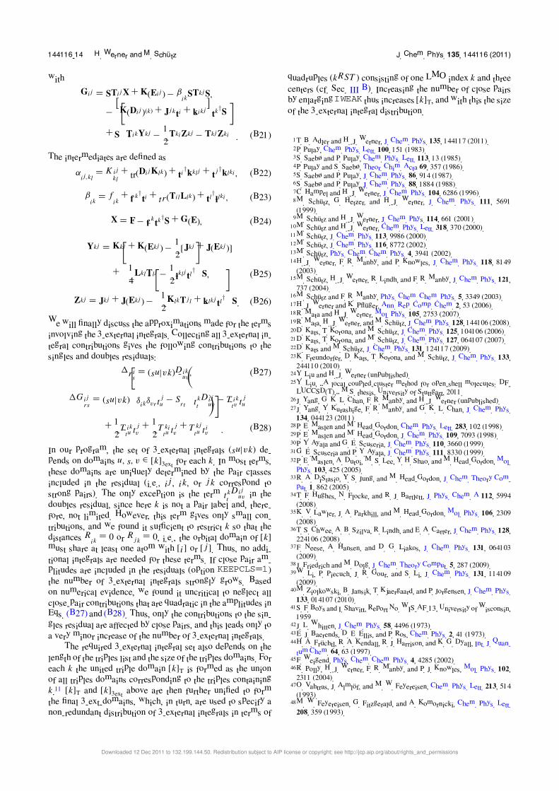
144116-14 H. Werner and M. Schütz J. Chem. Phys. 135, 144116 (2011)
with
Gij = STijX + K(Eij ) − βikSTkjS,
−�
K(Dij )(k) + Jjkti + kikj�
tk†S
+S
�
TikYkj −1
2TkiZkj − TkjZki
�
. (B21)
The intermediates are defined as
αij,kl = Kij
kl + tr(DijKlk) + ti†kklj + tj
†klki , (B22)
βik = fik + f k†ti + tr(TilLlk) + tl
†llki , (B23)
X = F − fktk†S + G(E), (B24)
Ykj = Kkj + K(Ekj ) −1
2[Jkj + J(Ekj )]
+
�
1
4LklTlj −
1
2lklj tl
†�
S, (B25)
Zkj = Jkj + J(Ekj ) −
�
1
2KlkTj l + klkj tl
†�
S. (B26)
We will finally discuss the approximations made for the terms
involving the 3-external integrals. Collecting all 3-external in-
tegral contributions gives the following contributions to the
singles and doubles residuals:
�ris = (su|vk)Dikuv, (B27)
�Gijrs = (su|vk)
�
δikδvr tju − Srt
�
t kt Dijuv − T ik
tv tju
+1
2T iktu t
jv +
1
2T kitu t
jv + T
kjtu t iv
��
. (B28)
In our program, the set of 3-external integrals (su|vk) de-
pends on domains u, s, v ∈ [k]3ext for each k. In most terms,
these domains are uniquely determined by the pair classes
included in the residual (i.e., ij , ik, or jk correspond to
strong pairs). The only exception is the term tkt Dijuv in the
doubles residual, since here k is not a pair label and, there-
fore, not limited. However, this term gives only small con-
tributions, and we found it sufficient to restrict k so that the
distances Rik = 0 or Rjk = 0, i.e., the orbital domain of [k]
must share at least one atom with [i] or [j ]. Thus, no addi-
tional integrals are needed for these terms. If close pair am-
plitudes are included in the residuals (option KEEPCLS=1)
the number of 3-external integrals strongly grows. Based
on numerical evidence, we found it uncritical to neglect all
close-pair contributions that are quadratic in the amplitudes in
Eqs. (B27) and (B28). Thus, only the contributions to the sin-
gles residual are affected by close pairs, and this leads only to
a very minor increase of the number of 3-external integrals.
The required 3-external integral set also depends on the
length of the triples list and the size of the triples domains. For
each k the united triple domain [k]T is formed as the union
of all triples domains corresponding to the triples containing
k.11 [k]T and [k]3ext above are then further unified to form
the final 3-ext-domains, which, in turn, are used to specify a
non-redundant distribution of 3-external integrals in terms of
quadruples (kRST ) consisting of one LMO index k and three
centers (cf. Sec. III B). Increasing the number of close pairs
by enlarging IWEAK thus increases [k]T, and with this the size
of the 3-external integral distribution.
1T. B. Adler and H.-J. Werner, J. Chem. Phys. 135, 144117 (2011).2P. Pulay, Chem. Phys. Lett. 100, 151 (1983).3S. Saebø and P. Pulay, Chem. Phys. Lett. 113, 13 (1985).4P. Pulay and S. Saebø, Theor. Chim. Acta 69, 357 (1986).5S. Saebø and P. Pulay, J. Chem. Phys. 86, 914 (1987).6S. Saebø and P. Pulay, J. Chem. Phys. 88, 1884 (1988).7C. Hampel and H.-J. Werner, J. Chem. Phys. 104, 6286 (1996).8M. Schütz, G. Hetzer, and H.-J. Werner, J. Chem. Phys. 111, 5691
(1999).9M. Schütz and H.-J. Werner, J. Chem. Phys. 114, 661 (2001).
10M. Schütz and H.-J. Werner, Chem. Phys. Lett. 318, 370 (2000).11M. Schütz, J. Chem. Phys. 113, 9986 (2000).12M. Schütz, J. Chem. Phys. 116, 8772 (2002).13M. Schütz, Phys. Chem. Chem. Phys. 4, 3941 (2002).14H.-J. Werner, F. R. Manby, and P. Knowles, J. Chem. Phys. 118, 8149
(2003).15M. Schütz, H.-J. Werner, R. Lindh, and F. R. Manby, J. Chem. Phys. 121,
737 (2004).16M. Schütz and F. R. Manby, Phys. Chem. Chem. Phys. 5, 3349 (2003).17H.-J. Werner and K. Pflüger, Ann. Rep. Comp. Chem. 2, 53 (2006).18R. Mata and H.-J. Werner, Mol. Phys. 105, 2753 (2007).19R. Mata, H.-J. Werner, and M. Schütz, J. Chem. Phys. 128, 144106 (2008).20D. Kats, T. Korona, and M. Schütz, J. Chem. Phys. 125, 104106 (2006).21D. Kats, T. Korona, and M. Schütz, J. Chem. Phys. 127, 064107 (2007).22D. Kats and M. Schütz, J. Chem. Phys. 131, 124117 (2009).23K. Freundorfer, D. Kats, T. Korona, and M. Schütz, J. Chem. Phys. 133,
244110 (2010).24Y. Liu and H.-J. Werner (unpublished).25Y. Liu, “A local coupled-cluster method for open-shell molecules: DF-
LUCCSD(T),” M.S. thesis, University of Stuttgart, 2011.26J. Yang, G. K. L. Chan, F. R. Manby, and H.-J. Werner (unpublished).27J. Yang, Y. Kurashige, F. R. Manby, and G. K. L. Chan, J. Chem. Phys.
134, 044123 (2011).28P. E. Maslen and M. Head-Gordon, Chem. Phys. Lett. 283, 102 (1998).29P. E. Maslen and M. Head-Gordon, J. Chem. Phys. 109, 7093 (1998).30P. Y. Ayala and G. E. Scuseria, J. Chem. Phys. 110, 3660 (1999).31G. E. Scuseria and P. Y. Ayala, J. Chem. Phys. 111, 8330 (1999).32P. E. Maslen, A. Dutoi, M. S. Lee, Y. H. Shao, and M. Head-Gordon, Mol.
Phys. 103, 425 (2005).33R. A. DiStasio, Y. S. Jung, and M. Head-Gordon, J. Chem. Theory Com-
put. 1, 862 (2005).34T. F. Hughes, N. Flocke, and R. J. Bartlett, J. Phys. Chem. A 112, 5994
(2008).35K. V. Lawler, J. A. Parkhill, and M. Head-Gordon, Mol. Phys. 106, 2309
(2008).36T. S. Chwee, A. B. Szilva, R. Lindh, and E. A. Carter, J. Chem. Phys. 128,
224106 (2008).37F. Neese, A. Hansen, and D. G. Liakos, J. Chem. Phys. 131, 064103
(2009).38J. Friedrich and M. Dolg, J. Chem. Theory Comput. 5, 287 (2009).39W. Li, P. Piecuch, J. R. Gour, and S. Li, J. Chem. Phys. 131, 114109
(2009).40M. Ziolkowski, B. Jansik, T. Kjaergaard, and P. Jorgensen, J. Chem. Phys.
133, 014107 (2010).41S. F. Boys and I. Shavitt, Report No. WIS-AF-13, University of Wisconsin,
1959.42J. L. Whitten, J. Chem. Phys. 58, 4496 (1973).43E. J. Baerends, D. E. Ellis, and P. Ros, Chem. Phys. 2, 41 (1973).44H. A. Früchtl, R. A. Kendall, R. J. Harrison, and K. G. Dyall, Int. J. Quan-
tum Chem. 64, 63 (1997).45F. Weigend, Phys. Chem. Chem. Phys. 4, 4285 (2002).46R. Polly, H.-J. Werner, F. R. Manby, and P. J. Knowles, Mol. Phys. 102,
2311 (2004).47O. Vahtras, J. Almlöf, and M. W. Feyereisen, Chem. Phys. Lett. 213, 514
(1993).48M. W. Feyereisen, G. Fitzgerald, and A. Komornicki, Chem. Phys. Lett.
208, 359 (1993).
Downloaded 12 Dec 2011 to 132.199.144.50. Redistribution subject to AIP license or copyright; see http://jcp.aip.org/about/rights_and_permissions
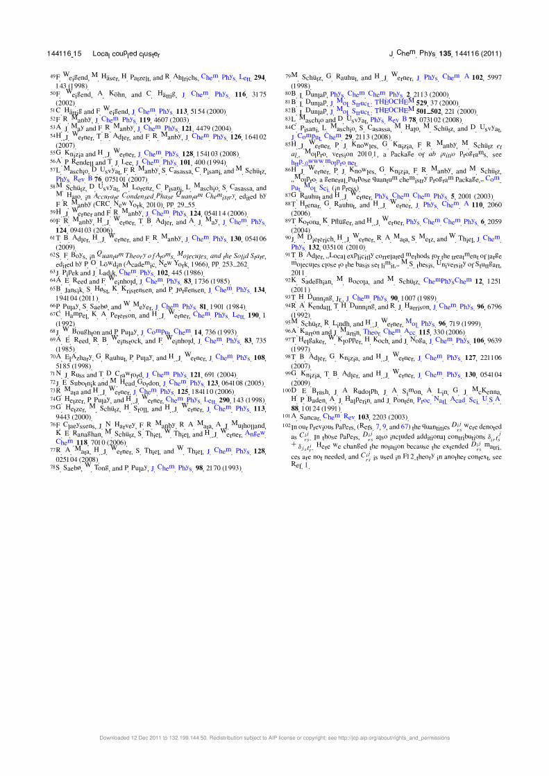
144116-15 Local coupled cluster J. Chem. Phys. 135, 144116 (2011)
49F. Weigend, M. Häser, H. Patzelt, and R. Ahlrichs, Chem. Phys. Lett. 294,
143 (1998).50F. Weigend, A. Köhn, and C. Hättig, J. Chem. Phys. 116, 3175
(2002).51C. Hättig and F. Weigend, J. Chem. Phys. 113, 5154 (2000).52F. R. Manby, J. Chem. Phys. 119, 4607 (2003).53A. J. May and F. R. Manby, J. Chem. Phys. 121, 4479 (2004).54H.-J. Werner, T. B. Adler, and F. R. Manby, J. Chem. Phys. 126, 164102
(2007).55G. Knizia and H.-J. Werner, J. Chem. Phys. 128, 154103 (2008).56A. P. Rendell and T. J. Lee, J. Chem. Phys. 101, 400 (1994).57L. Maschio, D. Usvyat, F. R. Manby, S. Casassa, C. Pisani, and M. Schütz,
Phys. Rev. B 76, 075101 (2007).58M. Schütz, D. Usvyat, M. Lorenz, C. Pisani, L. Maschio, S. Casassa, and
M. Halo, in Accurate Condensed-Phase Quantum Chemistry, edited by
F. R. Manby (CRC, New York, 2010), pp. 29–55.59H.-J. Werner and F. R. Manby, J. Chem. Phys. 124, 054114 (2006).60F. R. Manby, H.-J. Werner, T. B. Adler, and A. J. May, J. Chem. Phys.
124, 094103 (2006).61T. B. Adler, H.-J. Werner, and F. R. Manby, J. Chem. Phys. 130, 054106
(2009).62S. F. Boys, in Quantum Theory of Atoms, Molecules, and the Solid State,
edited by P. O. Löwdin (Academic, New York, 1966), pp. 253–262.63J. Pipek and J. Ladik, Chem. Phys. 102, 445 (1986).64A. E. Reed and F. Weinhold, J. Chem. Phys. 83, 1736 (1985).65B. Jansìk, S. Høst, K. Kristensen, and P. Jørgensen, J. Chem. Phys. 134,
194104 (2011).66P. Pulay, S. Saebø, and W. Meyer, J. Chem. Phys. 81, 1901 (1984).67C. Hampel, K. A. Peterson, and H.-J. Werner, Chem. Phys. Lett. 190, 1
(1992).68J. W. Boughton and P. Pulay, J. Comput. Chem. 14, 736 (1993).69A. E. Reed, R. B. Weinstock, and F. Weinhold, J. Chem. Phys. 83, 735
(1985).70A. ElAzhary, G. Rauhut, P. Pulay, and H.-J. Werner, J. Chem. Phys. 108,
5185 (1998).71N. J. Russ and T. D. Crawford, J. Chem. Phys. 121, 691 (2004).72J. E. Subotnik and M. Head-Gordon, J. Chem. Phys. 123, 064108 (2005).73R. Mata and H.-J. Werner, J. Chem. Phys. 125, 184110 (2006).74G. Hetzer, P. Pulay, and H.-J. Werner, Chem. Phys. Lett. 290, 143 (1998).75G. Hetzer, M. Schütz, H. Stoll, and H.-J. Werner, J. Chem. Phys. 113,
9443 (2000).76F. Claeyssens, J. N. Harvey, F. R. Manby, R. A. Mata, A. J. Mulholland,
K. E. Ranaghan, M. Schütz, S. Thiel, W. Thiel, and H.-J. Werner, Angew.
Chem. 118, 7010 (2006).77R. A. Mata, H.-J. Werner, S. Thiel, and W. Thiel, J. Chem. Phys. 128,
025104 (2008).78S. Saebø, W. Tong, and P. Pulay, J. Chem. Phys. 98, 2170 (1993).
79M. Schütz, G. Rauhut, and H.-J. Werner, J. Phys. Chem. A 102, 5997
(1998).80B. I. Dunlap, Phys. Chem. Chem. Phys. 2, 2113 (2000).81B. I. Dunlap, J. Mol. Struct.: THEOCHEM 529, 37 (2000).82B. I. Dunlap, J. Mol. Struct.: THEOCHEM 501–502, 221 (2000).83L. Maschio and D. Usvyat, Phys. Rev. B 78, 073102 (2008).84C. Pisani, L. Maschio, S. Casassa, M. Halo, M. Schütz, and D. Usvyat,
J. Comput. Chem. 29, 2113 (2008).85H.-J. Werner, P. J. Knowles, G. Knizia, F. R. Manby, M. Schütz et
al., Molpro, version 2010.1, a package of ab initio programs, see
http://www.molpro.net.86H.-J. Werner, P. J. Knowles, G. Knizia, F. R. Manby, and M. Schütz,
“Molpro: a general-purpose quantum chemistry program package,” Com-
put. Mol. Sci. (in press).87G. Rauhut and H.-J. Werner, Phys. Chem. Chem. Phys. 5, 2001 (2003).88T. Hrenar, G. Rauhut, and H.-J. Werner, J. Phys. Chem. A 110, 2060
(2006).89T. Korona, K. Pflüger, and H.-J. Werner, Phys. Chem. Chem. Phys. 6, 2059
(2004).90J. M. Dieterich, H.-J. Werner, R. A. Mata, S. Metz, and W. Thiel, J. Chem.
Phys. 132, 035101 (2010).91T. B. Adler, “Local explicitly correlated methods for the treatment of large
molecules close to the basis set limit,” M.S. thesis, University of Stuttgart,
2011.92K. Sadeghian, M. Bocola, and M. Schütz, ChemPhysChem 12, 1251
(2011).93T. H. Dunning, Jr., J. Chem. Phys. 90, 1007 (1989).94R. A. Kendall, T. H. Dunning, and R. J. Harrison, J. Chem. Phys. 96, 6796
(1992).95M. Schütz, R. Lindh, and H.-J. Werner, Mol. Phys. 96, 719 (1999).96A. Karton and J. Martin, Theor. Chem. Acc. 115, 330 (2006).97T. Helgaker, W. Klopper, H. Koch, and J. Noga, J. Chem. Phys. 106, 9639
(1997).98T. B. Adler, G. Knizia, and H.-J. Werner, J. Chem. Phys. 127, 221106
(2007).99G. Knizia, T. B. Adler, and H.-J. Werner, J. Chem. Phys. 130, 054104
(2009).100D. E. Brash, J. A. Rudolph, J. A. Simon, A. Lin, G. J. McKenna,
H. P. Baden, A. J. Halperin, and J. Pontén, Proc. Natl. Acad. Sci. U.S.A.
88, 10124 (1991).101A. Sancar, Chem. Rev. 103, 2203 (2003).102In our previous papers, (Refs. 7, 9, and 67) the quantities D
ijrs were denoted
as Cijrs . In those papers, D
ijrs also included additional contributions δir t
js
+ δjs tir . Here we changed the notation because the extended D
ijrs matri-
ces are not needed, and Cijrs is used in F12-theory in another context, see
Ref. 1.
Downloaded 12 Dec 2011 to 132.199.144.50. Redistribution subject to AIP license or copyright; see http://jcp.aip.org/about/rights_and_permissions