an efficient heuristic ordering algorithm for partial matrix refactorization

-.__ IEEE Transactions on Power Systems, Vol. 3, No. 3, August 1988 l a -

AN EFFICIENT HEURISTIC ORDERING ALGORITHM FOR PARTIAL MATRIX REFACTORIZATION

Ram& Betancourt San Diego State University

San Diego CA, 92182

ABSTRACT. An efficient algorithm for ordering a sparse matrix A for partiaI refactorization is given. simple graph manipulations. The method locally minimizes the length of the factorization paths while preserving the sparsity of the matrix. The ordering method is also useful in enhancing the sparsity of the inverse of the triangular factor L of A, and in other applications. Claims are substantiated by experiments using test data from several power systems networks and comparison with conventional ordering techniques.

The heuristic ordering method is based on

I INTRODUCTION

In order to analyze many practical problems of power systems it is necessary to use a sparse system of n equations in the form

The first step is factoring the A matrix as:

A x = b (1)

A = L U (2)

followed by forward and back substitution operations On the vector b. If A is symmetric it is decomposed as LDLt, where D is diagonal and Lt is the transpose of L.

Very often the conditions of the problem are such that some of the elements of the matrix require modification. A complete refactorization of the matrix is the sim- plest method but it is also most expensive. Chang and Brandwajn 111 recently presented efficient methods in which only certain elements of the matrix factors are updated. In their work, the solution process is modeled . by a graph, called the factorization path graph. This graph shows the row/columns of the matrix that only require modification when changes occur.

The matrices that represent power networks are very sparse and usually do not have a discernible structure. Different orderings of these matrices produce different numbers of fill-ins and factorization path graphs. To minimize the total execution time of the partial refactorization process, it is necessary to decrease the number of

87 SM 445-0 by the IEEE Power System Engineering Committee of the IEEE Power Engineering Society for presentation at the IEEEIPES 1987 Summer Meeting, San Francisco, California, July 12 - 17, 1987. Manuscript submitted January 28, 1987; made available for printing May 19, 1987.

A paper recommended and approved

row/columns that need to be modified. This is equivalent to decreasing the length of the factorization paths. Shorter paths might require more fill-ins, greater complexity and expense. Optimal use of computer time and resources can be obtained only by reordering these matrices to minimize both fill-ins and path lengths. To meet this objective, an heuristic procedure for ordering the matrix is proposed. This procedure will attempt to minimize the length of the paths while preserving the sparsity of the matrix. The method also has other applications such as improving the sparsity of the inverse of L, in parallel processing and in trfdiagonal matrices. This study is limited to symmetric, positive definitive matrices and the bus incidence matrix of a system is used here as an example.

I1 REVIEW OF ORDERING AND FACTORIZATION PATH GRAPHS.

a) Conventional Ordering of Matrices. Most of the extensive studies on the

sparse matrix reordering problem have been concerned with the minimization of the fill- ins [Zl. The only algorithms of practical interest are those which can produce good orderings in relative rapid execution time since true global optimal ordering of a matrix is conjectured to be an NP-problem [ 3 ? . The following algorithm, which emerged quite early in sparsity applications [ 4 1 , still seems to be the best for power system networks: Minimum Degree Algorithm (Tinney's Second Scheme). (1) Order the variables so that at each

step of the factorization the row of the variable to be eliminated has the fewest nonzero elements.

(2) When two or more variables satisfy this criterion, the choice is arbitrary.

Other methods like the Cuthill-Mckee Algorithm and the Nested Dissection Algo- rithm have also been applied to network matrices. Experience and investigation [5,61 have established the Minimum Degree Algo- rithm as the best compromise between speed and efficiency. Reference [21 explains de- tails of this algorithm.

Interpretation of the effects of ordering on sparsity by use of an undirected graph can be helpful in developing ordering schemes and implementing computer programs [71. A power system network may be thought of as being its own graph. For any other symmetric matrix with an arbitrary sparsity pattern the undirected graph is generated according to the following rule: For each pair of nonzero, nondiagonal elements a in

ij

0885-8950/88/08001181$01 .WO1988 IEEE

1182

A, there corresponds an undirected edge joining vertices i and j in the undirected graph. The elimination of a variable from the matrix corresponds to the elimination of a vertex from the graph. When a vertex is eliminated, the connectivity that existed prior to its elimination must be preserved. This may require the addition of new edges to the reduced graph. The new edges correspond to the fill-in terms in the matrix.

b) The Factorization Path Graph. The factorization paths of a matrix were

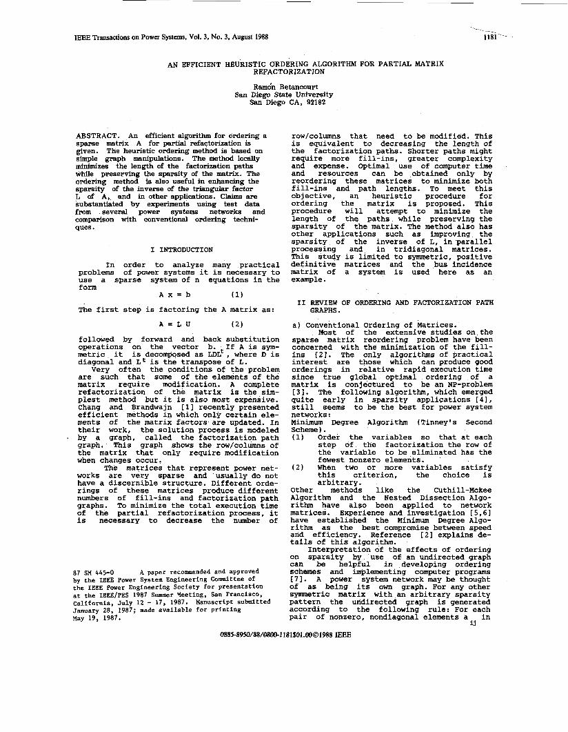
first introduced with respect to sparse vector operations to expose the precedence relations that exists among operations on row/columns of the matrix [81 . The factorization path for any specific column k of the matrix is an ordered list of columns of L starting at k. The list has the number of the row of the first nonzero element in column k. This new row is then taken as a column and the process is repeated until the last node is reached (node n). The factorization paths are modeled by a graph in which the nodes represent the row/columns of A. This graph is referred to as the factorization path graph. For example, the factored admittance matrix of the ten-node system of Figure 1.a has the sparsity structure given in Figure 1.b. The Minimum Degree Algorithm is used in this case and the factorization process produces one fill- in. The correspon-ding factorization path graph is shown in Figure 2. As indicated in 111 the modification of a

row/column of matrix A affects only a specific number of ascending row/columns in A and complete refactorization can be avoided. The affected row/columns are found from the factorization path graph of the matrix. For example, if the elements of row/column c are modified then, as shown in Figure 2, only row/columns d,e ..,j need to be refactored.

of node i in the factorization path is defined as the path length from node i to an initial node in the same path. The lengths for the nodes in Figure 2 are given to the right of the graph. The maximum length in this case is 1 = 9. The following section presents an ordering algorithm desig- ned to reduce the length of these paths so that a smaller number of row/columns need to be refactored while preserving the sparsity of the matrix.

The length li

111 ORDERING ALGORITHM FOR MINIMUM PATH LENGTHS

An important observation is that during the elimination process, the remaining diagonal elements in the reduced matrix determine the length of the path in the kth step of the factorization. Also, assume that a is chosen as the kth pivot and that aipayi # o in the reduced matrix. Then the length li corresponding to the diagonal aii at the kth step is given by

li = max{lp + 1, % I ( 3 )

x x c x x d x x x e f

x x x x x

? x x x x

X X F X X x x

6) X Original Element F Fill-in Element

Figure 1. (a) A ten-node exwple network. (b) Sparsity structure of matrix L.

Length

0 P 1 t 2

8

Figure 2. The factorization path graph using the Minimum Degree Algorithm.

where 1, is the length of the pivot at the time of its elimination. These observations suggest that the lengths of the paths can be determined using the undirected graph of the matrix. First, the vertices in the undirected graph start with a "length" set to zero. When a vertex is eliminated the lengths of its adjacent vertices are updated using Eqn. 3 . The process continues until all the vertices are eliminated. The length of the vertex at the time of its elimination is equal to the length of its path on the factorization path graph. This concept (length of the vertex) is similar to the "degree" concept used for sparsity presarva- tion.

1183

C 9

h d j f .

With this technique, a new ordering algorithm can be outlined. In this case, the general criteria are the lengths of the vertices in the undirected graph rather than the number of edges connected to the vertices (degree). This algorithm can be called the Minimum Length Algorithm as compared to its equivalent , the Minidm Degree Algorithm. Minimum Length Algorithm. (i) Order the vertices so that at each

step of the process the vertex to be eliminated has the lowest length.

(ii) When two or more vertices satisfy this criterion the choice is arbitrary.

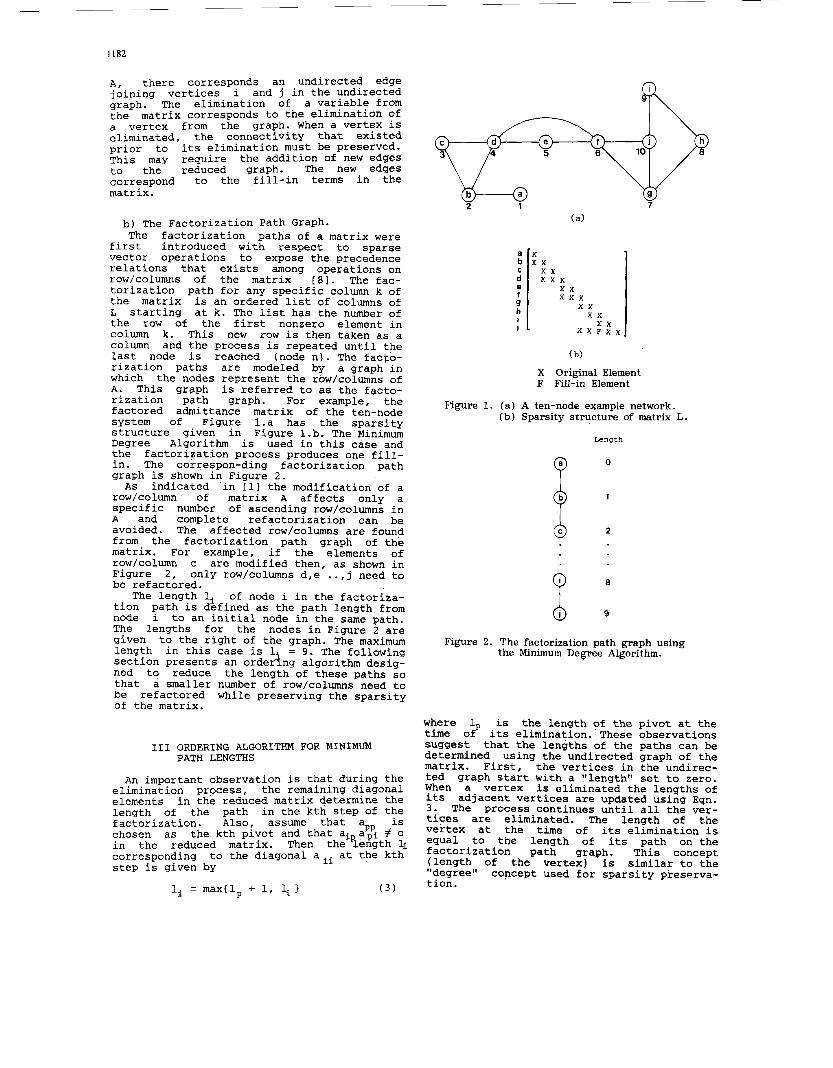
As all the vertices start with 1 0 the selection of the first node is arbitriry. As an illustration of the Minimum Length Algo- rithm, consider again the system in Figure 1. The way the algorithm is carried out for this example is shown in Figure 3. The results of this ordering are shown in the matrix of Figure 4.a and the corresponding factorization path graph is given in Figure 4.b. In this case, the modification of row/column c affects only row/columns b, d, and f instead of six row/columns with the ordering given by the Minimum Degree. On the other hand, row/column i in Figure 2 only needed to refactor one more element, but in Figure 4 , it required three. In most practical cases the row/columns that will be modified are randomly determined by the problem, otherwise a special ordering can be used. In the case Qf Figure 2 the mean length of the paths is 4.5 with a standard deviation of 3.02. In Figure 4 these quantities are 2.1 and 1.19 respectively. This shows a significant improvement in the length of the paths.

Minimizing the length alone does not lead to the greatest efficiency, as additional fill-ins may be generated. This would require performance of an increased number of arithmetical operations. Also, the lengths may increase due to the increased number of non-zero elements. Matrix reordering for the most economical partial refactorization thus requires minimizing both length and fill-in. Two general strategies are feasible:

Strategy A: Minimum Degree, Minimum Length

(i) Pick the next vertex using Minimum Degree.

(ii) Break a tie using Minimum Length. (iii) If more than one vertex qualifies,

break the tie arbitrarily.

Strategy B: Minimum Length, Minimum Degree (ML-MD)

(i) Pick the next vertex using Minimum

(ii) Break a tie using Minimum Degree. (iii) If more than one vertex qualifies,

For example, when strategy A is applied to the system in Figure 1! it produces the triangulation path graph in Figure 5 and one fill-in. Strategy B gives the same ordering in this case as the one in Figure 4.

(MD-ML ) 4

Length.

break a tie arbitrarily.

a x e x I X

X X

b X X X x x x

x x x x X X F X

X X F X X X

Figure 3. Ordering of A using the Minimum Length Algorithm. Bold lines indicate fill-ins. The number by the vertex indicates the length of the node.

Length

Figure 4. (a) Sparsity (b) structure of matrift L using the Minimum Length Algorithm.

(b) The factorization path graph.

1184

Length

0

2

y 1 3

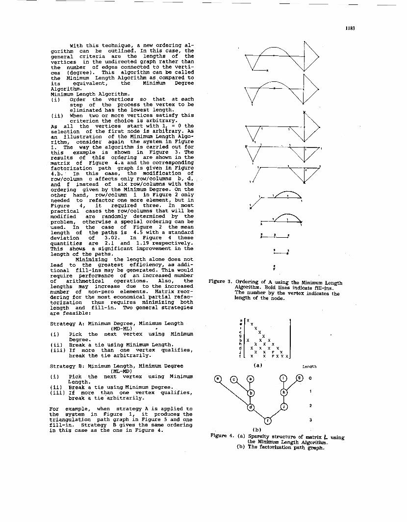
Figure 5. The factorization path graph using the MD-ML method.

IV EXPERIMENTAL RESULTS

The ordering strategies proposed need to be evaluated by experimentation as they are heuristic in nature. The aim is to achieve the "best compromise" between the statistics of the factorization paths and the number of fill-ins created. Three test networks have been chosen which are typical of the power industry. Test case one is a 118 node matrix which is a IEEE standard test case. Test cases two and three are a 1084 and a 1993 node matrices corresponding to systems within the Western System Coordinated Council (WSCC).

Table I shows the results of the ordering strategies on these matrices. For comparison, the results of applying the Minimum Degree and the Minimum Length Algorithms are also given in the Table. The Minimum Length Algorithm does not always give the best results, since the method does not consider the excessive fill-ins that are being generated in the matrix, eventually "slowing down" the process. The ML-MD Algorithm appears to cause the smallest standard deviation of the four but the number of fill-ins is comparatively high. The Table indicates that the MD-ML Method is the best option. The number of fill-ins is basically the same as with the Minimum Degree Algorithm but the average length and standard deviation of the factorization paths are significantly reduced. Application of the MD-ML method to the three test cases required about 1.5%, 2.0% and 3.1% more CPU time than application of the Minimum Degree algorithm. The method was easily implemented by slight modification of an existing Minimum Degree ordering routine.

The orderings given by the Minimum Degree and the MD-ML algorithms were tested in a partial refactorization program. A sin- gle line modification was simulated over 35% of two test cases at randomly chosen posi- tions. Since the number of fill-ins created by both methods is basically the same, the CPU time for a complete factorization is also the same. This time is taken as the base unit when comparing these methods and the results are summarized in Table 11. This Table clearly illustrates the performance attainable with the technique presented in this paper. Using the new ordering technique the mean number of operations required for partial refactorization has been reduced by more than 25%, and the standard deviation is reduced about 50%.

Mean Path Std. Dev. Longest Path Fill-ins



MD MD-ML ML ML-MD

size = 118

11.56 8.23 15.94 8.14 4.72 2.25 4.76 2.19

23 12 20 11 84 85 386 107

size = 1084

27.93 20.67 45.15 21.45 7.88 4.41 12.76 4.31

51 29 61 27 1041 1033 4121 1509

size = 1993

45.57 35.66 88.80 39.58 14.93 8.48 23.56 8.18

92 52 2725 45 2579 2590 12874 3487

MD = Minimum Degree ML = Minimum Length

TABLE I. Comparison of ordering schemes: length of factorization paths.

size = 118 = 1084

Mean CPU TIME % 32.27 23.90 18.98 14.01 Std. Dev. % l y 4 6 MDi:17 1 ::34 ""rl:l

TABLE 11. Comparison of ordering schemes: partial refactorization.

V FURTHER APPLICATIONS

a. Inversion of L. Given equation (l), we may write

x = A-lb (4)

x = ( LDLt ) -lb (5)

with

w = L-1 then

(7) x = Wt D-'W b

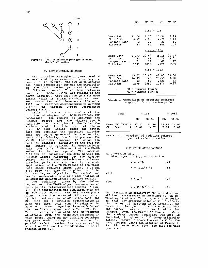
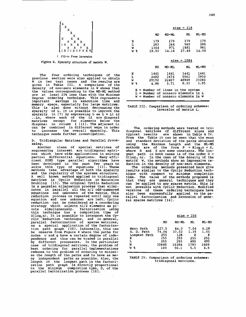
The matrix W is relatively sparse and it was utilized extensively in reference 191 in several applications. It is important to reali- ze that any ordering selected for L affects the number of fill-ins in W. Actually, the nodes in the path of node k coincide with the nonzero rows of column k of W. For example, when the matrix in Figure 1, where the Minimum Degree algorithm was used, is inverted, it gives a full lower triangular matrix. Figure 6 shows the matrix W for the same system using the ordering of Figure 3. In this case only five new fill-ins were generated.

1185

X X

X X

x x x I X x x x I X I I X I F X X X

X

x x x X X F X

I Fill-in From Inversion

Figure 6 . Sparsity structure of matrix W.

The four ordering techniques of the previous section were also applied to obtain W in two test cases and the results are given in Table 111. A comparison of the density of non-zero elements in W shows that the values corresponding to the MD-ML method are at least 25% less than with the Minimum Degree ordering technique. This represents important savings in execution time and memory space, especially for large matrices. This is also done without decreasing the sparsity of L. It is p'ossible to improve the sparsity in (7) by expressing L as L = L 1 L2 ..Ln, where each of the Li are diagonal matrices except for elements below the diagonal in column i [ll]. The adjacent Li can be combined in different ways in order to increase the overall sparsity. This technique needs further investigation.

b. Tridiangular Matrices and Parallel Proce- ssing.

Another class of special matrices of engineering interest are tridiagonal matrices which have wide applications in solving partial differential equations. Many efficient SIMD type parallel algorithms have been developed in the past few years to solve this type of equations [12]. These methods take advantage of both the sparsity and the regularity of the systems structure. A well known method applied to tridiagonal matrices is Cyclic Reduction or Recursive Doubling [131. The original Cyclic Reduction is a gaussian elimination process that elimi- nates in parallel all the n/2 odd-numbered equations and unknowns of the matrix. This reduction process is repeated until only one equation and one unknown are left. Cyclic reduction can be considered as a reordering strategy which selects ni/2 elements as pi- vots simultaneously. Factorization using this technique has a completion time of O(log2n). It is possible to interpret the Cy- clic Reduction technique, and in general, parallel factorization of sparse matrices, as a special application of the factorization path graph [lo]. Informally, this can be observe from Figure 4 where the paths for nodes c and g have a certain degree of inde- pendence and thus can be traced in parallel by different processors. In the particular case of tridiagonal matrices, the problem of best ordering for parallel implementations reduces to the problem of ordering to minimize the length of the paths and to have as many independent paths as possible. Also, the length of the longest path in the factorization path graph is directly proportional to the minimum completion time, D, of the parallel factorization process [lo].

MD

E 179 L 263 w 1364 W % 19.92

MD

E 1441 L 2482 W 29192 W % 4.98

size = 118

MD-ML ML

179 179 264 565 971 1881

14.18 27.49

size = 1084

MD-ML ML

1441 1441 2474 5562

22407 48949 3.71 8.33

ML-MD

179 286 961

14.04

ML-MD

1441 2950

23260 3.95

E = Number of lines in the system L = Number of nonzero elements in L W = Number of nonzero elements in W

TABLE 111. Comparison of ordering schemes: inversion of matrix L.

The ordering methods were tested on tridiagonal matrices of different sizes and typical results are shown in Table # IV. From the Table it can be seen that the mean and standard deviation of the paths obtained using the Minimum Length and the ML-MD methods ?re of the form P = Rlog n + S, where R and S are some constants. Tie longest path in both cases is of the order D = O(log2 n). In the case of the density of the matrix W, the methods show an impressive reduction in the density of non-zero elements.

The ordering methods presented here give results similar to the Cyclic Reduction technique with respect to minimum completion time. The value of the methods proposed is that they are general techniques and they can be applied to any sparse matrix. This is not possible with Cyclic Reduction. Modified versions of these ordering techniques have also been successfully applied to the parallel factorization and inversion of general sparse matrices 1141.

MD

Mean Path 127.5 S. D. Path 74.04 Longest Path 255 E 255 L 255 W 32640 W % 100

size = 256

MD-ML ML ML-MD

64.0 7.04 6.28 37.02 1.39 1.55 128 8 8 255 255 255 255 495 495

16384 1793 1609 50.1 5.5 4.9

TABLE IV. Comparison of ordering schemes: tridiagonal matrices.

1186

3c. Other ordering schemes. In most of problems associated with po-

wer system networks, the matrix A has the property that pivoting may be performed on diagonal elements in any order without ad- versely affecting numerical accuracy. This favorable property allows the establishment of the ordering without the row and column exchanges needed in general pivot selection techniques. Taking advantage of this, it is possible to outline a set of equivalent ordering schemes similar to the ones previous- ly proposed when considering only sparsity preservation [4]. For example, the equivalent to the ordering scheme 3 or Minimum Deficiency Algorithm would be: Scheme 3': Order the nodes so that at each

step of the factorization, the node to be eliminated introduces the lowest new length on its adjacent nodes. When two or more nodes satisfy this criterion, the choice is arbitrary.

The Minimum Deficiency algorithm is not wi- dely used to solve practical problems since its implementation is cumbersome and difficult compared to the Minimum Degree. Also, the overhead in terms of execution time appears to be large. It is conjectured here that the implementation of the equivalent scheme has similar characteristics but it may be effective for other systems of equations and new types of problems.

VI CONCLUSION

A locally optimal algorithm has been proposed for an efficient partial refactorization of a sparse matrix. It is described in terms of ordering the undirected graph associated with the matrix by use of graph transformations. At each step the vertex selected is the one that minimizes both the fill-ins and the length of the factorization path. The method has been shown to be very effective on the matrices considered in this study. A comparison of the results derived from the methods studied here, emphasizes the merits of the new technique. Applying this method to the inversion of matrlx L reduces the nonzero elements significantly. At first glance the new method may appear to be a valance tie breaker, but it is not. This can be seen from the application of the method to tridiagonal matrices. In this case, traditional cyclic reduction can be considered as a special application of Minimum Length algorithm. The method is competitive with and in some instances superior .CO the best methods currently in use 1151. Its value justifies the additional time required for its execution.

ACKNOWLEDGMENTS

The author would like to thank William Torre of the San Diego Gas and Electric Co. who provided the test cases used in the paper. Lauren Outland from Cal. State L. A. provided helpful discussions and editorial comments.

REFERENCES

[l] S. M. Chang and V. Brandwajn: "Partial Matrix Refactorization", IEEE Trans. on Power Systems, Vol. PWRS-1, No 1, February 1986, pp. 193-200.

[2] A. George and J. W. Liu: "Computer of Large Sparse Positive Defi-

[3] D. J. Rose and R. E. Tarjan: "Algorithmic Aspects of Vertex Elimination in Directed Graphs", SIAM J. Appl. Math. 1978, 34, (1) pp.176-197

[4] N. Sat0 and W. F. Tinney: 'Techniques for Exploiting the Sparsity of the Network Admittance Matrix', IEEE Trans. PAS, Vol. 82, December 1963, pp. 944-50

[5] J. G. Lewis and W. G. Poole: "Ordering Algorithms Applied to Sparse Matrices in Electrical Power Problems" in A. M. Erisman, K. W. Neves, and M. H. Dwarakanath: "Electric Power Problems: the Mathematical Challenge", SIAM, 1980, pp. 115-124.

[6] I. S. Duff and J. K. Reid: "A Comparison of Sparsity Orderings for Obtaining a Pivotal Sequence in Gaussian Elimination", J. Inst. Math. E, Appl. 1974, 14, pp. 281-291.

Solution nitive Systems", Prentice-Hall, 1981.

[7] W. R. Spillers and N. Hickerson: "Optimal Elimination for Sparse Symmetric Systems as Graph Problem". Quartely Journal of App 1 ied Mathematics, Vol. 26, No 3, 1968.

[81 W. F. Tinney, V. Brandwajn and S. M. Chang: "Sparse Vector Methods" , IEEE Trans. PAS-104, No. 2, February 1985,

[91 0. Alsac, B. Stott, and W. F. Tinney: "Sparsity-Oriented Compensation Methods for Modified Solutions," IEEE Trans. on PAS, May 1983, pp. 1050-1060

[lo] R. Betancourt and F. L. Alvarado: of Sparse "Parallel 1 nver s ion

Matrices", IEEE Trans. on Power Systems, Vol. PWRS-1, No. 1, Feb. 1986,

[ll] J. E. Van Ness and G. Molina: The Use of Multiple Factoring in the Parallel Sclution of Algebraic Equations", IEEE Trans. PAS, October 1983, pp 3433-3438.

[12] A. H. Sameh and D. J. Kuck: "Parallel Direct Linear System Solvers - a Survey", in: "Parallel Computers - Parallel Mathematics", M. Felmuer (Edit.), North Holland, 1977, pp.25-30.

pp. 295-301.

pp. 74-81.

[13] H. S. Stone: "Parallel Tridiagonal Equa- tions Solvers", ACM Trans. Math. Software, 1975, 1, pp. 289-307.

[14] R. Betancourt: "Efficient Parallel Processing Technique for Inverting Matrices with Random Sparsity", IEE Proc. Vol. 133, Pt. E, No 4, July 1986,

[151 R. Betancourt, discussion to: A. Gomez and L. Franquelo: "Node Ordering Algorithms for Sparse Vector Method ImPrOVement", IEEE Power Eng. SOC.

pp. 235-240.

Winter Meeting, New Orleans , Louisiana, Feb. 1987.

1187

Discussion

R. Mota-Palomino (hstituto Politknico Nacional, M6xico): The author is to be commended for a timely paper on heuristic orderings for efficient partial matrix refactorization.

Recently other researchers [A] have reported heuristic orderings to improve the efficiency of sparse vector methods and have claimed to improve the sparsity of the triangular factors of a sparse matrix by using very simple “tie-breaking” rules in Tinney’s Ordering (scheme 2). In this paper the author proposes different heuristic orderings that shorten the sparse matrix factorization paths but that affect the sparsity of its triangular factors, hence suggesting that some “tie-breaking” rule should also be applied in combination with Tinney’s Ordering (scheme 2). Would the author like to comment on the connection between the ordering he is proposing and those reported in [A]?

In section 3-c of the paper the author mentions other ordering schemes, particularly orderings combined with Tinney’s scheme 3 (or the minimum deficiency algorithm). Would the author care to clarify this idea? Does the author have any experience working with other ordering schemes that only take sparsity’into account? I would like to congratulate the author for his continuous effort in searching for efficient computational techniques to solve power system problems.

Reference

[A] A. Wmez and L. G. Franquelo, “Node ordering algorithms for sparse vector method improvement,” IEEE Trans. Power Sysf., Vol. 3, No. 1, February 1988, pp. 73-79.

Manuscript received August 11, 1987.

R. Betancourt: The author wishes to thank Dr. Mota-Palomino for his comments and questions.

The essential idea behind algorithm AI of [15] is the use of the past history of the node as the tie breaker for the MD algorithm. When a tie occurs, it selects the node with the fewest adjacent nodes already e l i t e d . A preliminary comparison is made of the A1 and the MD-ML methods in a discussion to [15]. Table V gives the results of applying A1 to the examples used in this paper. This table clearly shows that the method proposed in the paper is superior to A1 since it gives shorter path lengths and standard deviations. The computer time required by both methods is essentially the same.

TABLE V Comparison of Ordering Schemes: The A1 Method

size 118 1084 1993 Fill-ins 85 1275 2644 Mean Path 9.17 25.15 40.62 std. Dev. 2.98 5.55 9.49

In response to the second question, it is interesting to note the similarities in effort and results of these new methods with the three classical ordering schemes [4]. It is not difficult to imagine method A1 as equivalent to scheme 1 . Both use the number of lines connected to the node either on the original graph or on the filled graph [lq. Also, the complexity and the final comparative results are similar.

The analogy between scheme 2 and ML was mentioned in the paper. Other ordering algorithms “equivalent” to scheme 3 are possible, most of them based on the structure of matrix W. For example, the nonzero entries in column i of W give nodes that are included in the path of node i. This is essentially the basis of the ML algorithm. But the nonzero entries in row i of Wgive the nodes that are above node i in the path graph; that is, the nodes in which path node i is included. For instance, row d in the matrix of Fig. 6 has nonzero elements in columns a, e, c, and b. These are the nodes above node din Fig. 4.b. A different set of heuristics can then be based on this last observation.

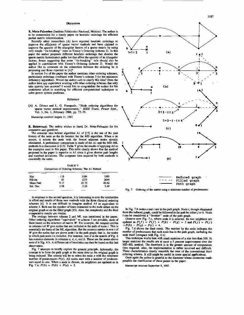
Fig. 7 attempts to briefly explain the general principle. Informally, the concept is to form the path graph at the same time as the original graph is being reduced. The criteria will be to select the node x with the minimm number of predecessors P(x). AU nodes start with a number of predecessors equal to one. When a node is chosen, its neighbors are updated as in Fig. 7.a: P(b) = P(b) + P(a) = 2.

l + l = 2 1 t! ‘ ‘\

u 3 I

I.,

I /- Reduced graph Filled graph Path graph

- - - - -

Fig. 7. Ordering of the matrix using a minimum number of predecessors.

In Fig. 7.b nodes U and c are in the path graph. Node i, though eliminated from the reduced graph, could be followed in the path be either j or h. Node i can be considered a “frontier” node of the path graph.

Observe now Fig. 7.c, where node h is selected. Its two qeighbors are

Fig. 7.d shows the final result. The number by the node indicates the number of predecessors that each node has in the path graph, including the node itself (compare with Fig. 4.b).

This technique works best with small matrices of a size less than 500. In larger matrices the results are at most a 5 percent improvement over the MD-ML method. The drawback is in the greater amount of computation time required. Also, the implemenWon is rather involved and difficult. These charac@ristics closely resemble the ones of the conventional third ordering scheme. It still might be useful in some special applications.

Once again the author is grateful to the discusser whose comments made possible the clarification of these points in the paper. Manuscript nceived September 8, 1987.

updated as P(f) = P!f) + P ( h ) - P(g) = 5 and P ( j ) = P ( j ) + P ( h ) - P(g) - P ( l ) = 4.

an efficient heuristic ordering algorithm for partial matrix refactorization

Documents