IEEE TRANSACTIONS ON COMPUTERS, OCTOBER 1975

Condition 2:

ai+n ai+n-1 * a,oao(llb)

&n bn1l * @ bo

i.e., the nonzero msd's are aligned.

Condition 3:

ai+n+i ai+n ai+n1 *... ai *ao(llc)

&n bn_1 ... bo

i.e., the nonzero msd of b is placed one digit right of a or the re-mainder.When Condition 3 exists, the polarized addition is always pos-

sible, while when Condition 2 exists, the polarized addition is neverpossible. When Condition 1 exists, the decision is slightly compli-cated. First obtain Pcri as

Pcri=b (1--+-2-- An) (12)

and take ai+n_l and msd of Pc, for comparison and follow thefollowing steps (for detailed proof, see [10]).

Step 1: Compare the digits under consideration. If the digit ofPcri is smaller, the polarized addition is possible; if larger, polarizedaddition is not possible; and if equal, go to Step 2.

Step 2: If all the digits have already been compared, go to Step 5;otherwise go to Step 3.

Step 3: Compare next digits. If the digit of P,,i is larger, thepolarized addition is possible; if smaller, polarized addition is notpossible; and if equal, go to Step 4.

Step 4: If the comparison of all the digits have already beencompleted, go to Step 5; otherwise take next significant digits forcomparison and go to Step 1.

Step 3: Take qi = 0, qi-l = 0 and onwards alternate digits as(3- 1) and 0. Final remainder will be zero.

The results of division thus obtained, will have a unique representa-tion in -# base and the possibilities of initial overflow and qi = +,8(as happens in nonstoring division algorithms proposed by Sankaret at. [1]) have been completely eliminated and Conditions 2, 3,and Step 5 behaves as a deterministic algorithm. It is worth men-tioning that, once P,,i has been evaluated for any specific "i," samevalue, with proper right shift, can be utilized for onwards computa-tion of lower significant digits. But value of qi-2 and onward digitsof Step 5, will no longer hold good.

VI. SQUARE-ROOT

The difference of this process from division lies in the fact thatthe subtrahend changes in successive step of square-rooting. Here,an algorithm which generates polarized addend (rather than subtra-hend) is given. The method starts with the selection of (1 ,B-1)as the two digits of the first polarized addend and allow its addition.Onward addend can be evaluated with the help of the followingsteps.

Step A: Add (1 8 -2) to the previous addend, with the lsd'saligned. Take the result as a new addend and go to Step B.

Step B: If possible, add the polarized addend and go to Step A;otherwise go to Step C.

Step C: Add (2 ,B-1) to the previous addend, with 2 alignedwith the lsd of the previous addend, shift the result one digit toright and take the result as a new addend and go to Step B. (In thecase of base -2, take the equivalent value 1 1 0 1.)

The square-rooting process is similar to the division operationand therefore details are not given here. For this operation Pcrt hasto be taken as present value of polarized addend plus (1 1), with

the msd of the second aligned with the lsd of first. Also, Step 5 hasto be taken as qi = 1, qi-l = (3 - 1) and onwards digits and re-mainder as zero. (For detailed proof, refer to [10].)The possibility of getting either positive or negative root, has

already been mentioned by Sankar et al. Square-rooting will givepositive root only when (m + 1)/2 is odd (m is the number ofdigits of a). If it is even and it is still desired to obtain the positiveroot directly, the position of the initial polarized addend has to beshifted through two digits, either to the left or to the right and thecondition for left shift is given below.

Condition for Left Shift: Take w = B3-1 0 63-1 0 ... withtotal number of digits equal to (m - 1)/2; obtain the square of wand use it as Peri and if comparison allows polarized addition inStep 1 or 3, allow the left shift; otherwise right shift. When m = 1,always do left-shift, while evaluating negative root.

VII. CONCLUSION

Faster and more general algorithms for arithmetic operations in anegative radix, have been described in this correspondence and anattempt has been made to solve the problems associated with divi-sion and square-rooting operation.

REFERENCES

[1] P. V. Sankar, S. Chakrabarti, and E. V. Krishnamurthy, "Arith-metic algorithms in a negative base," IEEE Trans. Comput., vol.C-22, pp. 120-125, Feb. 1973.

[2] S. Zohar, "New hardware realizations of nonrecursive digitalfilters," IEEE Trans. Comput., vol. 0-22, pp. 328-338, Apr. 1973.

[3] , "The counting recursive digital filter," IEEE Trans. Comput.,vol. C-22, pp. 338-347, Apr. 1973.

[4] , "Fast hardware Fourier transformation through counting,"IEEE Trans. Comput., vol. C-22, pp. 433-441, May 1973.

[51 - , "A/D conversion for radix (-2)," IEEE Trans. Comput.,vol. C-22, pp. 698-701, July 1973.

[6] D. V. Kanani and K. H. O'Keefe, "A note on conditional-sumaddition for base -2 systems," IEEE Trans. Comput. (Corresp.),vol. C-22, p. 626, June 1973.

[7] L. S. Houselander, "Cellular-array negabinary multiplier," Electron.Lett., vol. 10, pp. 168-169, May 1974.

[8] D. P. Agrawal, "Negabinary carry-look-ahead adder and fastmultiplier," Electron. Lett., vol. 10, pp. 312-313, July 1974.

[9] -, "Negabinary complex number multiplier," Electron. Lett.,vol. 10, pp. 502-503, Nov. 1974.

[10] , "Some aspects of fast arithmetic techniques," Ph.D. dis-sertation, Fed. Inst. Technol., Lausanne, Switzerland, 1975.

An Algorithm for Finding Nearest Neighbors

JEROME H. FRIEDMAN, FOREST BASKETT, ANDLEONARD J. SHUSTEK

Abstract-An algorithm that finds the k nearest neighbors of apoint, from a sample of size N in a d-dimensional space, with anexpected number of distance calculations

E[nd] $ 2r E2[kdr (d/2) ]iId(2N)1-(lId)is described, its properties examined, and the validity of the estimateverified with simulated data.

Manuscript received June 24, 1974; revised February 7, 1975. Thiswork was supported in part by the U. S. Atomic Energy Commissionunder Contract AT(043)515.

J. H. Friedman is with Stanford Linear Accelerator Center, Stanford,Calif. 94305.

F. Baskett and L. J. Shustek are with the Computer Science Depart-ment, Stanford University, Stanford, Calif.

1000

CORRESPONDENCE

Index Terms-Best match, nearest neighbors, nonparametricdiscrimination, searching, sorting.

INTRODUCTION

Nearest-neighbor techniques have been shown to be importantnonparametric procedures for multivariate density estimation andpattern classification [1]-[6]. For classification, a sample of proto-type feature vectors is drawn from each category, correctly labeledby an external source. For each test point to be classified, the set ofk closest prototype points (feature vectors) is found and the testpoint is assigned to that category having the largest representationin this set. For density estimation, the volume, V(k), containingthe closest k points to each of the N sample points, is used to esti-mate the local sparsity s (inverse density) by s = NV(k) Ik - 1.The application of these techniques has been severely limited by

the computational resources required for finding the nearest neigh-bors. The feature vectors for the complete set of samples must bestored, and the distances to them calculated for each classificationor density estimation. Several modifications to the k-nearest-neighborrule have been suggested that are computationally more tractablebut whose statistical properties are unknown [7], [8]. The con-densed nearest-neighbor rule [9] mitigates both the storage andprocessing requirements by choosing a subset of the prototypevectors such that the nearest-neighbor rule correctly classifies all ofthe original prototypes.

Fisher and Patrick [10] suggest a preprocessing scheme for reduc-ing the computational requirements of nearest-neighbor classifica-tions when the test sample is much larger than the prototype set.For this case, it is worthwhile to use considerable computationpreprocessing the prototypes so that processing can be reduced foreach test sample. Their technique orders the prototypes so thateach point tends to be far away from its predecessors in the orderedlist. By examining these prototype points in this order and havingprecalculated distances between prototypes, the triangle inequalitycan be applied to eliminate distance calculations from the testvector to many of the prototypes. (All of the prototypes must beexamined, however.) The algorithm is examined only for k = 1 intwo dimensions where for bivariate normal data a median numberof approximately 58 distance calculations is required for 1000 proto-types, after preprocessing.

This correspondence describes a straightforward preprocessingtechnique for reducing the computation required for finding the knearest neighbors to a point from a sample of size N in a d-dimen-sional space. This procedure can be profitably applied to both densityestimation and classification, even when the number of test pointsis considerably smaller than the number of prototypes. This pre-processing requires no distance calculations. (It can, however, re-quire up to dNlog2 N comparisons.) The distance function (dis-similarity measure) is not required to satisfy the triangle inequality.With a Eucidean distance measure' the average number of proto-types that need be examined is bounded by

(1)after preprocessing.For the case of bivariate normal data with d = 2, k = 1, and

N = 1000, (1) predicts an average of 36 distance calculations,whereas simulations have shown that 24 are actually required. Theperformance of the algorithm is compared to (1), with simulateddata for several values of k, d, N, and underlying density distribu-tions of the prototype sample points.

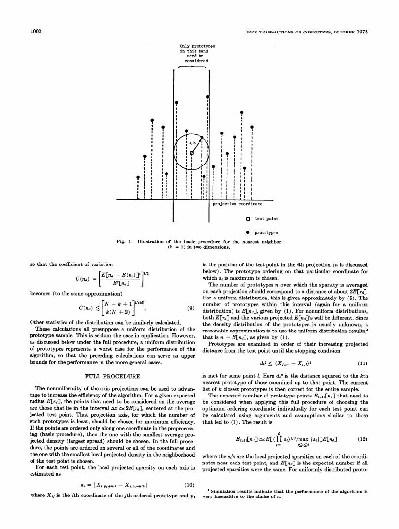
each test point, the prototypes are examined in the order of theirprojected distance from the test point on the sorted coordinate.When this projected distance becomes larger than the distance (inthe full dimensionality) to the k closest point of those prototypesalready examined, no more prototypes need be considered; the kclosest prototypes of the examined points are those for the completeset. Fig. 1 illustrates this procedure for the nearest neighbor (k = 1)in two dimensions.A simple calculation gives an approximation to the expected

number of prototypes that need be examined before the abovestopping criterion is met. For simplicity, consider N prototypesuniformly distributed in a d-dimensional unit hypercube and aEuclidean distance measure. Assume also that N is large enough sothat effects due to the boundaries are not important. For this case,the volume v of a d-dimensional sphere, centered at the test pointand containing exactly k-prototypes, is a random variable distrib-uted according to a beta distribution

()N!p(v) dv = (k - 1)!(N - k)!vkl(1- V)N-kdv, 0 < v < 1. (2)

The radius of this sphere, given by

rdr (d/2) ji/drd L ,27d/2 V (3)

is also a random variable. Let

rd=[2ird12/dr (d/2) ]Id.

Then v = (rdrd)d and the distribution for rd becomes

p (rd) drd = (k 1)!(N - k)! (¢drd)dk1[l1 - (¢drd)d]Nkdrd. (4)The stopping criterion is met when the projected distance from thetest point to a prototype along the sorted coordinate is greater thanrd. This projected distance is uniformly distributed. The expectedfraction of prototypes, then, that must be examined is just twicethe expected value of rd given by (4) . Various other statistics, suchas the variance, median, and percentiles, can also be calculated from(4). These calculations must be done numerically since the integralscannot be evaluated analytically.A close upper bound3 on E[rd] can be derived from (2) and (3) by

r[2(d/2) l[v d

E[rdI<Lrd =

2irdl2E Jv

where from (2),

E[v] =N + 1 (6)

The upper bound on the expected fraction of prototypes that mustbe examined is then 2rd, and the upper bound on the expected numberof prototypes E[nd] is 2;dN. Combining these results,

d <d/2*) k l]ldE[nd] n' =2 N.

[27rd/2 N +1J(7)

Simplifying this expression and approximating N + 1 by N, one hasthe result shown in (1). The variance of nd is similarly approxi-mated by

F/dr (d/2) 2 k(N-k+ 1) Id

E[nd- E(nd)]2<4 [\2wxd12 )(N+1)2(N +2)JN (8)

BASIC PROCEDURE

The preprocessing for this algorithm consists basically of orderingthe prototype points on the values of one of the coordinates. For

I Similar formulas for other distance measures are discussed below.

2 Prototypes must be examined for a projected distance rd both aboveand below the test point position.

3 Taking the dth root of the average rather than the average of thedth root will cause a slight overestimation that decreases with increasingd. For d = 2, this overestimation is around 10 percent, while for d = 8it is 6 percent.

1001

(5)

E[n4j< 7r-112P%l Ekd1P (d/2) ]l1d (2N) 1-(I/d),

IEEE TRANSACTIONS ON COMPUTERS, OCTOBER 1975

Only prototypesin this band

need beconsidered

0 test point

0 prototypes

Fig. 1. Illustration of the basic procedure for the nearest neighbor(k = 1) in two dimensions.

so that the coefficient of variation

C(nd) =[[nE[in2]I[ Pnd] ]

becomes (to the same approximation)

C[(nd) k([ + 2) ]

Other statistics of the distribution can be similarly calculated.These calculations all presuppose a uniform distribution of the

prototype sample. This is seldom the case in application. However,as discussed below under the full procedure, a uniform distributionof prototypes represents a worst case for the performance of thealgorithm, so that the preceding calculations can serve as upperbounds for the performance in the more general cases.

FULL PROCEDURE

The nonuniformity of the axis projections can be used to advan-tage to increase the efficiency of the algorithm. For a given expectedradius E[rd], the points that need to be considered on the averageare those that lie in the interval Ax - 2E[rd], centered at the pro-jected test point. That projection axis, for which the number ofsuch prototypes is least, should be chosen for maximum efficiency.If the points are ordered only along one coordinate in the preprocess-ing (basic procedure), then the one with the smallest average pro-jected density (largest spread) should be chosen. In the full proce-dure, the points are ordered on several or all of the coordinates andthe one with the smallest local projected density in the neighborhoodof the test point is chosen.For each test point, the local projected sparsity on each axis is

estimated as

Si =I Xi,pi+n/2 - Xipi-n/21 (10)

is the position of the test point in the ith projection (n is discussedbelow). The prototype ordering on that particular coordinate forwhich si is maximum is chosen.The number of prototypes n over which the sparsity is averaged

on each projection should correspond to a distance of about 2E[rd].For a uniform distribution, this is given approximately by (5). Thenumber of prototypes within this interval (again for a uniformdistribution) is E[nd], given by (1). For nonuniform distributions,both E[rd] and the various projected E[nd]'s will be different. Sincethe density distribution of the prototypes is usually unknown, areasonable approximation is to use the uniform distribution results,4that is n = E[nd], as given by (1).

Prototypes are examined in order of their increasing projecteddistance from the test point until the stopping condition

dk2< (Xi,pi -X,,1)2 (11)

is met for some point 1. Here de2 is the distance squared to the kthnearest prototype of those examined up to that point. The currentlist of k closest prototypes is then correct for the entire sample.The expected number of prototype points Efull[nd] that need to

be considered when applying this full procedure of choosing theoptimum ordering coordinate individually for each test point canbe calculated using arguments and assumptions similar to thosethat led to (1). The result is

d

EfiulEnd] E[(H si) "d/max {si 1 ]E[nd]i-1 I<i<d

(12)

where the si's are the local projected sparsities on each of the coordi-nates near each test point, and E[nd] is the expected number if allprojected sparsities were the same. For uniformly distributed proto-

4 Simulation results indicate that the performance of the algorithm isvery insensitivre to the choice of n1.where Xii is the ith coordinate of the jth ordered prototype and pi

1002

0

I II II

III II

t

IIII

IIII

CORRESPONDENCE

1.000

zw

u

LL 0.100LL z

> Z

I-

< 0.010

0.001100 1000

N10000

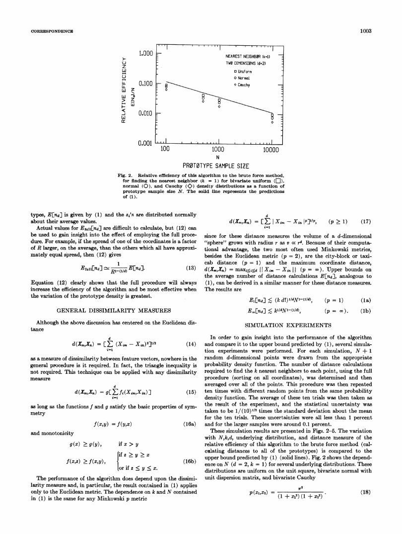
PR0T0TYPE SAMPLE SIZEFig. 2. Relative efficiency of this algorithm to the brute force method,

for flnding the nearest neighbor (k = 1) for bivariate uniform (f),normal (0), and Cauchy ($) density distributions as a function ofprototype sample size N. The solid line represents the predictionsof (1).

types, E[nd] is given by (1) and the si's are distributed normallyabout their average values.

Actual values for Efll[End] are difficult to calculate, but (12) can

be used to gain insight into the effect of employing the full proce-dure. For example, if the spread of one of the coordinates is a factorof R larger, on the average, than the others which all have approxi-mately equal spread, then (12) gives

1

Bf,,iind] - RX(ld EEnd]- (13)R1-(iId)

Equation (12) clearly shows that the full procedure will alwaysincrease the efficiency of the algorithm and be most effective whenthe variation of the prototype density is greatest.

d

d(Xm,Xn) = E Xim- Xin lP]J/P,i-I

(p > 1) (17)

since for these distance measures the volume of a d-dimensional"sphere" grows with radius r as v cc rd. Because of their computa-tional advantage, the two most often used Minkowski metrics,besides the Euclidean metric (p = 2), are the city-block or taxi-cab distance (p = 1) and the maximum coordinate distance,d(Xm,Xn) = maXlid I Xim- Xin (p = o). Upper bounds on

the average number of distance calculations E[nd], analogous to(1), can be derived in a similar manner for these distance measures.The results are

Ei[nd] < (kd!)1/dNl-(lId), (P = 1) (la)

GENERAL DISSIMILARITY MEASURES E n[nd] $< klIdNi-(ld), (p = on). (lb)

Although the above discussion has centered on the Euclidean dis-tance

d(Xm,Xn) (Xim -Xin)2]1/2 (14)i'-1

as a measure of dissimilarity between feature vectors, nowhere in thegeneral procedure is it required. In fact, the triangle inequality isnot required. This technique can be applied with any dissimilaritymeasure

d

d (Xm,Xn) = 9[ fi (Xim,Xin) ] (15)i=l

as long as the functions f and g satisfy the basic properties of sym-

metry

f(x,y) = f(y,x) (16a)and monotonicity

g(x) .g(y), if x > y

f(x,z) > f(x,y),if z > y > x

or if z < y < x.

The performance of the algorithm does depend upon the dissimi-larity measure and, in particular, the result contained in (1) appliesonly to the Euclidean metric. The dependence on k and N containedin (1) is the same for any Minkowski p metric

SIMULATION EXPERIMENTS

In order to gain insight into the performance of the algorithmand compare it to the upper bound predicted by (1), several simula-tion experiments were performed. For each simulation, N + 1random d-dimensional points were drawn from the appropriateprobability density function. The number of distance calculationsrequired to find the k nearest neighbors to each point, using the fullprocedure (sorting on all coordinates), was determined and thenaveraged over all of the points. This procedure was then repeatedten times with different random points from the same probabilitydensity function. The average of these ten trials was then taken as

the result of the experiment, and the statistical uncertainty was

taken to be 1/(10) 12 times the standard deviation about the mean

for the ten trials. These uncertainties were all less than 1 percentand for the larger samples were around 0.1 percent.These simulation results are presented in Figs. 2-5. The variation

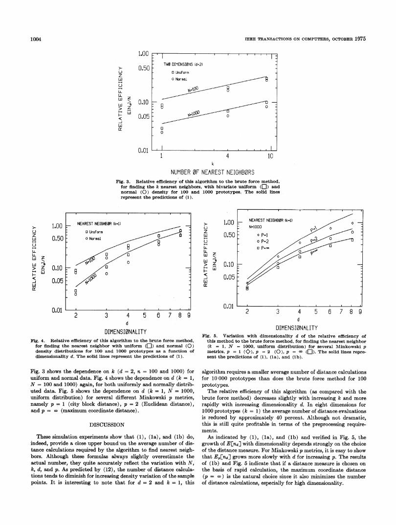
with N,k,d, underlying distribution, and distance measure of therelative efficiency of this algorithm to the brute force method (cal-calating distances to all of the prototypes) is compared to theupper bound predicted by (1) (solid lines). Fig. 2 shows the depend-ence on N (d = 2, k = 1) for several underlying distributions. Thesedistributions are uniform on the unit square, bivariate normal withunit dispersion matrix, and bivariate Cauchy

p(Xl,x2) = ( + X12) (1 + X2') (18)

NEAREST NEIGHB0R (k=i)TW0 DIMENSIONS (d=2)

O UniFormO Normal

- Cauchy _

I ~~~~ :

1003

IEEE TRANSACTIONS ON COMPUTERS, OCTOBER 1975

1.00

z

-I_LiLL

F---JlI

0.50

z

zLU

0.10

0.05

0.011 4 10

k

NUMBER 0F NEAREST NEIGHB0RSFig. 3. Relative efflciency of this algorithm to the brute force method,

for finding the k nearest neighbors, with bivariate uniform (]) andnormal (0) density for 100 and 1000 prototypes. The solid linesrepresent the predictions of (1).

1.00

0.50

z"I

"1zLU

0.10

0.05

0.012 3 4 5 6 7 8 9

d

DIMENSI0NALITYFig. 4. Relative efficiency of this algorithm to the brute force method,

for finding the nearest neighbor with uniform ([) and normal (0)density distributions for 100 and 1000 prototypes as a function ofdimensionality d. The solid lines represent the predictions of (1).

Fig. 3 shows the dependence on k (d = 2, n = 100 and 1000) foruniform and normal data. Fig. 4 shows the dependence on d (k = 1,N = 100 and 1000) again, for both uniformly and normally distrib-uted data. Fig. 5 shows the dependence on d (k = 1, N = 1000,uniform distribution) for several different Minkowski p metrics,namely p 1 (city block distance), p = 2 (Eucidean distance),and p = o (maximum coordinate distance).

DISCUSSION

These simulation experiments show that (1), (la), and (lb) do,indeed, provide a close upper bound Non the average number of dis-tance calculations required by the algorithm to find nearest neigh-bors. Although these formulas always slightly overestimate theactual number, they quite accurately reflect the variation with N,k, d, and p. As predicted by (12), the number of distance calcula-tions tends to diminish for increasing density variation of the samplepoints. It is interesting to note that for d = 2 and k = 1, this

z

LULLLL

r-J

1LU

1.00

0.50

z

zLL

0.10

0.05

0.01

d

DIMENSI0NALITYFig. 5. Variation with dimensionality d of the relative efficiency of

this method to the brute force method, for flnding the nearest neighbor(k = 1, N = 1000, uniform distribution) for several Minkowski pmetrics, p = 1 (0), p = 2 (0), p = co (E). The solid lines repre-

sent the predictions of (1), (la), and (lb).

algorithm requires a smaller average number of distance calculationsfor 10000 prototypes than does the brute force method for 100prototypes.The relative efficiency of this algorithm (as compared with the

brute force method) decreases slightly with increasing k and more

rapidly with increasing dimensionality d. In eight dimensions for1000 prototypes (k = 1) the average number of distance evaluationsis reduced by approximately 40 percent. Although not dramatic,this is still quite profitable in terms of the preprocessing require-ments.As indicated by (1), (la), and (ib) and verified in Fig. 5, the

growth of E[nd] with dimensionality depends strongly on the choiceof the distance measure. For Minkowski p metrics, it is easy to showthat E,[nd] grows more slowly with d for increasing p. The resultsof (lb) and Fig. 5 indicate that if a distance measure is chosen on

the basis of rapid calculation, the maximum coordinate distance(p = co) is the natural choice since it also minimizes the numberof distance calculations, especially for high dimensionality.

I :TW0 DIMENSIONS (d=2)

o UniFormo NormlHi °~~~~8 0-00 0~~0

0~~~~~~~

0

0

CzH

U-4HLULL

-JH

LU

NEAREST NEIGHBffR (k=l)

O UniformO Normal

0

0

- 0.0

1004

CORRESPONDENCE

A crude calculation gives a rough idea of how many test pointsNt are required (in terms of the number of prototypes Np, k, and d)for the preprocessing procedure to be profitable. The preprocessingrequires approximately dN, log2 N, compares, memory fetches, andstores. Each distance calculation requires around d multiplies, sub-tractions, additions, and memory fetches. Assuming all of theseoperations require equal computation, then the preprocessing re-quires about 3dN, log N, operations, while it saves approximately4 dNj (N, - EEndl) operations. Thus, for the procedure to be profit-able

4dNj (Nv - E[nd]) > 3dNp, log N,,

1.00

,_

Ir-

C)

LD-

0.50

0.10

0.05or crudely5

Nt > No N, log2N,Np, E[nd]

(19)

EEnd] is given approximately by (1) (Euclidean metric). For d = 2,k = 1, and 1000 prototypes, No is around 10, whereas for d = 8,k = 1, and 1000 prototypes, one has No - 25.

Although these results are quite crude, it is clear that the numberof test points need not be large, compared to the number of proto-types, before the algorithm can be profitably applied. For densityestimation, where Nt = N2, = N, the procedure is profitable so longas No/N is small compared to one.

The only adjustable parameter in this algorithm is the number ofprojection coordinates m on which the data are sorted. This param-eter can range in value from one (basic procedure) to d (full proce-dure). The value chosen for this parameter is governed principallyby the amount of memory available. This algorithm requires mNadditional memory locations, and for m = d, doubles the memoryover that required by the brute force method. If less than the fullprocedure is employed, then those axes with the largest spreadshould be chosen. Arguments similar to those that lead to (13) can

be used to estimate the efficiency for this case. For the case whereall coordinates have approximately equal spread, (12) can be usedto show that the increase in efficiency, as additional sorted coordi-nates are added, is proportional to 1/m. Results of simulations (notshown) verify this dependence.The tendency toward decreasing relative efficiency with increas-

ing dimensionality cannot be mitigated by requiring the distancemeasure to satisfy the triangle inequality

d(xm,Xn) > d(Xm,xi) - d(xi,x.) (20)

In this case distance calculations can be avoided for those proto-types x. for which

d(X(,Xk) < d(xt,xt) - d(xi,x,,) (21)

2 3 4 5 6 7 8 9d

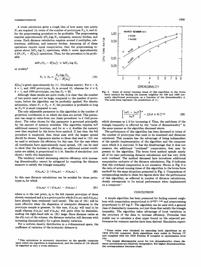
DIMENSI0NALITYFig. 6. Ratio of actual running times of this algorithm to the brute

force method for finding the nearest neighbor for 100 and 1000 nor-mally distributed prototypes, as a function of the dimensionality d.The solid lines represent the predictions of (1).

(rdl) (rd)2]1/2= [d(d ±+2)7j "(22)

which decreases as 1/d for increasing d. Thus, the usefulness of thetriangle inequality is affected by the "curse of dimensionality" inthe same manner as the algorithm discussed above.The performance of this algorithm has been discussed in terms of

the number of prototypes that need to be examined and distancescalculated. This measure has the advantage of being independentof the specific implementation of the algorithm and the computerupon which it is executed. It has the disadvantage that it does notmeasure the additional "overhead" computation that may bepresent in the algorithm. The brute force method spends nearlyall of its time performing distance calculations and has very littlesuch overhead. The method discussed here introduces additionalcomputation exclusive of the distance calculations. Fig. 6 indicatesthat this overhead computation is not excessive. Shown in Fig. 6 isthe ratio of actual running times of this algorithm to the brute forcemethods for the same situations presented in Fig. 4. Comparisons ofcorresponding results in these two figures show that the performanceof this algorithm, as reflected in number of distance calculations,closely corresponds to its actual performance when implementedon a computer.7

where x1 is the test point, Xk is the kth nearest prototype of thosealready examined and xi is a prototype for which d (xt,xj) and d (xj,xnlhave already been evaluated (and saved). The use of (21) will bemost effective when the dispersion of interpoint distances in theprototype sample is greatest. In this case, d(xt,xk) will tend to besmall whereas d(xt,xz) and d(xz,xn) will quite often be dissimilar,making the right-hand side on (21) large. Since distance varies as

the dth root of the volume, the distance variation will decrease withincreasing dimensionality for a given density variation.

For a uniform density distribution in a d-dimensional space, thecoefficient of variation of the interpoint distance is

This calculation is extremely dependent on the specific computerupon which the algorithm is implemented, and the results of (19) shouldbe regarded as only a crude estimate.

CONCLUSION

A simple algorithm has been presented for finding nearest neigh-bors with computation proportional to klldNl-(ld) and preprocessingproportional to dN log N. The algorithm can be used with a generalclass of dissimilarity measures, not just those that satisfy the triangleinequality. The algorithm takes advantage of local variations inthe structure of the data to increase efficiency. Formulas thatenable one to calculate a close upper bound on the expected per-

formance for common metrics have been derived. Simulation experi-

These ratios were obtained by executing both algorithms on anIBM 370/168 computer. Both algorithms were coded in Fortran IVand compiled with the IBM Fortran H compiler at optimization leveltwo.

7 The largest discrepancies occur for low dimensionality where dis-

tance calculations are relatively inexpensive. For higher dimensionalities,the correspondence becomes closer.

NEAREST NEIGHBOR (k-Dl

O N-lOOo N-lOOO

o

1005

0

IEEE TRANSACTIONS ON COMPUTERS, OCTOBER 1975

ments have been presented that illustrate the degree to which theseformulas bound the actual performance. g (x)

ACKNOWLEDGMENT

The authors would like to thank W. H. Rogers, S. Steppel, andJ. E. Zolnowsky for helpful discussions.

REFERENCES

[1] E. Fix and J. L. Hodges, Jr., "Discriminatory analysis; small sampleperformance," USAF School of Aviation Medicine, Randolf Field,Tex., Project 21-49-004, Rep. 11, Aug. 1952.

12] D. 0. Loftsgaarden and C. P. Quesenberry, "A nonparametricdensity function," Ann. Math Statist., vol. 36, pp. 1049-1051, 1965.

13] T. M. Cover and P. E. Hart, "Nearest neighbor pattern classifica-tion," IEEE Trans. Inform. Theory, vol. IT-13, pp. 21-27, Jan.1967.

[4] T. M. Cover, "Rates of convergence of nearest neighbor decisionprocedures," in Proc. 1st Annu. Hawaii Conf. Systems Theory, Jan.1968, pp. 413-415.

[5] T. J. Wagner, "Convergence of the neare3t neighbor rule," IEEETrans. Inform. Theory, vol. IT-17, pp. 566-571, Sept. 1971.

[6] K. Fukunaga and L. D. Hostetler, "Optimization of k-nearest-neighbor density estimates," IEEE Trans. Inform. Theory, vol.IT-19, pp. 320-326, May 1973.

[7] C. Barns, "An easily mechanized scheme for an adaptive patternrecognizer," IEEE Trans. Electron. Comput. (Corresp.), vol. EC-15,pp. 385-387, June 1966.

[8] E. A. Patrick and F. P. Fisher, "Generalized k-nearest neighbordecision rule," J. Inform. Contr., vol. 16, pp. 128-152, Apr. 1970.

[9] P. E. Hart, "The condensed nearest neighbor rule," IEEE Trans.Inform. Theory (Corresp.), vol. IT-14, pp. 515-516, May 1968.

[10] F. P. Fisher and E. A. Patrick, "A preprocessing algorithm fornearest neighbor decision rules," in Proc. Nat. Electronics Conf.,vol. 26, Dec. 1970, pp. 481-485.

II~~~~~~~~~~~~~~~~~~~~~~~~~~~~~~IL I

I I

I I

1 -x Ix -w0 x0 xo+vw-l

(a)

E (k, x)

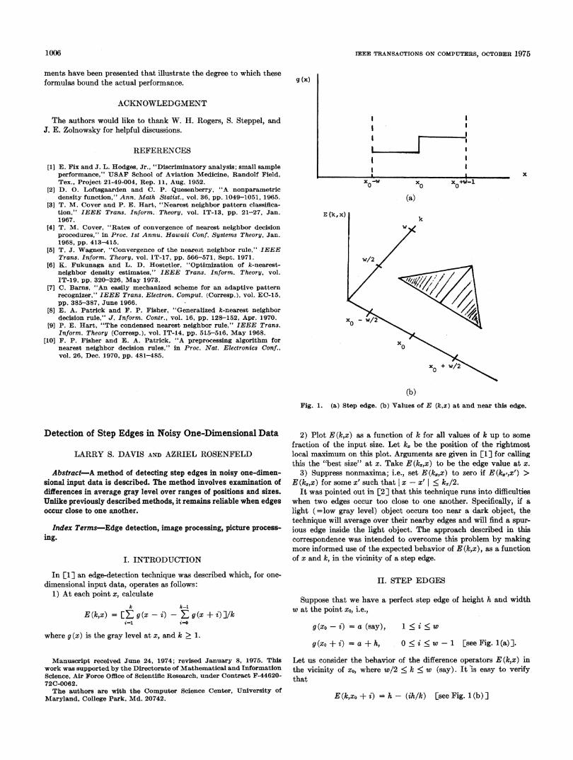
(b)Fig. 1. (a) Step edge. (b) Values of E (k,x) at and near this edge.

Detection of Step Edges in Noisy One-Dimensional Data

LARRY S. DAVIS AND AZRIEL ROSENFELD

Abstract-A method of detecting step edges in noisy one-dimen-sional input data is described. The method involves examination ofdifferences in average gray level over ranges of positions and sizes.Unlike previously described methods, it remains reliable when edgesoccur close to one another.

Index Terms-Edge detection, image processing, picture process-ing.

I. INTRODUCTION

In [1] an edge-detection technique was described which, for one-dimensional input data, operates as follows:

1) At each point x, calculatek k-1

E(k,x) = [E g(x-i) - Eg(x + i)]/ki=l i-S

where g(x) is the gray level at x, and k > 1.

2) Plot E (k,x) as a function of k for all values of k up to somefraction of the input size. Let kz be the position of -the rightmostlocal maximum on this plot. Arguments are given in [1] for callingthis the "best size" at x. Take E(kz,x) to be the edge value at x.

3) Suppress nonmaxima; i.e., set E (kz,x) to zero if E (k,',x') >E(kZ,x) for some x' such that x-x' < k,/2.

It was pointed out in [2] that this technique runs into difficultieswhen two edges occur too close to one another. Specifically, if alight (=low gray level) object occurs too near a dark object, the,technique will average over their nearby edges and will find a spur-ious edge inside the light object. The approach described in thiscorrespondence was intended to overcome this problem by makingmore informed use of the expected behavior of E(k,x), as a functionof x and k, in the vicinity of a step edge.

II. STEP EDGES

Suppose that we have a perfect step edge of height h and widthw at the point x0, i.e.,

g(xo-i) = a (say), 1 < i < w

g(xo+ i) = a + h, 0 < i < w-1 [see Fig. 1(a)].

Manuscript received June 24, 1974; revised January 8, 1975. Thiswork was supported by the Directorate of Mathematical and InformationScience, Air Force Office of Scientific Research, under Contract F-44620-72C-0062.The authors are with the Computer Science Center, University of

Maryland, College Park, Md. 20742.

Let us consider the behavior of the difference operators E (k,x) inthe vicinity of x0, where w/2 < k < w (say). It 'is easy to verifythat

E (k,xo + i) = h - (ihlk) [see Fig. 1 (b) ]

1006

I I