NASA/TM—2011–215974

AMT-200S Motor Glider Parameter and Performance Estimation

Brian R. Taylor

Dryden Flight Research Center, Edwards, California

Click here: Press F1 key (Windows) or Help key (Mac) for help

July 2011

https://ntrs.nasa.gov/search.jsp?R=20110015943 2018-07-17T17:16:29+00:00Z

NASA STI Program ... in Profile

Since its founding, NASA has been dedicated to the advancement of aeronautics and space science. The NASA scientific and technical information (STI) program plays a key part in helping NASA maintain this important role.

The NASA STI program operates under the auspices of the Agency Chief Information Officer. It collects, organizes, provides for archiving, and disseminates NASA’s STI. The NASA STI program provides access to the NASA Aeronautics and Space Database and its public interface, the NASA Technical Report Server, thus providing one of the largest collections of aeronautical and space science STI in the world. Results are published in both non-NASA channels and by NASA in the NASA STI Report Series, which includes the following report types:

• TECHNICAL PUBLICATION. Reports of

completed research or a major significant phase of research that present the results of NASA Programs and include extensive data or theoretical analysis. Includes compila- tions of significant scientific and technical data and information deemed to be of continuing reference value. NASA counter-part of peer-reviewed formal professional papers but has less stringent limitations on manuscript length and extent of graphic presentations.

• TECHNICAL MEMORANDUM. Scientific and technical findings that are preliminary or of specialized interest, e.g., quick release reports, working papers, and bibliographies that contain minimal annotation. Does not contain extensive analysis.

• CONTRACTOR REPORT. Scientific and technical findings by NASA-sponsored contractors and grantees.

• CONFERENCE PUBLICATION. Collected papers from scientific and technical conferences, symposia, seminars, or other meetings sponsored or co-sponsored by NASA.

• SPECIAL PUBLICATION. Scientific, technical, or historical information from NASA programs, projects, and missions, often concerned with subjects having substantial public interest.

• TECHNICAL TRANSLATION. English-language translations of foreign scientific and technical material pertinent to NASA’s mission.

Specialized services also include organizing and publishing research results, distributing specialized research announcements and feeds, providing help desk and personal search support, and enabling data exchange services.

For more information about the NASA STI program, see the following:

• Access the NASA STI program home page

at http://www.sti.nasa.gov

• E-mail your question via the Internet to help@sti.nasa.gov

• Fax your question to the NASA STI Help Desk at 443-757-5803

• Phone the NASA STI Help Desk at 443-757-5802

• Write to: NASA STI Help Desk NASA Center for AeroSpace Information 7115 Standard Drive Hanover, MD 21076-1320

This page is required and contains approved text that cannot be changed.

NASA/TM—2011–215974

AMT-200S Motor Glider Parameter and Performance Estimation

Brian R. Taylor

Dryden Flight Research Center, Edwards, California

Insert conference information, if applicable; otherwise delete

Click here: Press F1 key (Windows) or Help key (Mac) for help

National Aeronautics and Space Administration Dryden Flight Research Center Edwards, CA 93523-0273

July 2011

Enter acknowledgments here, if applicable.

NOTICE Use of trade names or names of manufacturers in this document does not constitute an official endorsement of such products or manufacturers, either expressed or implied, by the National Aeronautics and Space Administration.

Click here: Press F1 key (Windows) or Help key (Mac) for help

Available from:

Click here: Press F1 key (Windows) or Help key (Mac) for help

NASA Center for AeroSpace Information 7115 Standard Drive

Hanover, MD 21076-1320 443-757-5802

 

 

Abstract Parameter and performance estimation of an instrumented motor glider was conducted at the National Aeronautics and Space Administration Dryden Flight Research Center in order to provide the necessary information to create a simulation of the aircraft. An output-error technique was employed to generate estimates from doublet maneuvers, and performance estimates were compared with results from a well-known flight-test evaluation of the aircraft in order to provide a complete set of data. Aircraft specifications are given along with information concerning instrumentation, flight-test maneuvers flown, and the output-error technique. Discussion of Cramér-Rao bounds based on both white noise and colored noise assumptions is given. Results include aerodynamic parameter and performance estimates for a range of angles of attack.

Nomenclature an normal acceleration, g

anb normal acceleration bias, g ax axial acceleration, g

axb axial acceleration bias, g ay lateral acceleration, g

ayb lateral acceleration bias, g b reference span, ft C.G. center of gravity

CA total axial force coefficient

CAq axial force coefficient due to pitch rate

CA0 trim axial force coefficient

CAα axial force coefficient due to angle of attack

C

Aα2 axial force coefficient due to the square of the angle of attack

CAδe axial force coefficient due to elevator deflection

CD total coefficient of drag

CL total coefficient of lift

CL0 trim lift coefficient

CLα lift coefficient due to angle of attack (lift curve slope)

C

Lα2 lift coefficient due to the square of the angle of attack

Cl total rolling moment coefficient

Clp rolling moment coefficient due to roll rate

Clr rolling moment coefficient due to yaw rate

Cl0 trim rolling moment coefficient

Clβ rolling moment coefficient due to angle of sideslip

 

 

2

Clδa rolling moment coefficient due to aileron deflection

Clδ r rolling moment coefficient due to rudder deflection

Cm total pitching moment coefficient

Cmq pitching moment coefficient due to pitch rate

Cm0 trim pitching moment coefficient

Cmα pitching moment coefficient due to angle of attack

Cmδe pitching moment coefficient due to elevator deflection CN total normal force coefficient

CNq normal force coefficient due to pitch rate

CN0 trim normal force coefficient

CNα normal force coefficient due to angle of attack

C

Nα2 normal force coefficient due to the square of the angle of attack

CNδe normal force coefficient due to elevator deflection

Cn total yawing moment coefficient

Cnp yawing moment coefficient due to roll rate

Cnr yawing moment coefficient due to yaw rate

Cn0 trim yawing moment coefficient

Cnβ yawing moment coefficient due to angle of sideslip

Cnδa yawing moment coefficient due to aileron deflection

Cnδ r yawing moment coefficient due to rudder deflection CY total lateral force coefficient

CYdr lateral force coefficient due to rudder deflection

CYp lateral force coefficient due to roll rate

CYr lateral force coefficient due to yaw rate

CY0 trim lateral force coefficient

CYβ lateral force coefficient due to angle of sideslip

CYδa lateral force coefficient due to aileron deflection c reference chord, ft D axial displacement between main gear and tail wheel, ft FAA Federal Aviation Administration

FLM measured force at left main landing gear, lb

FRM measured force at right main landing gear, lb

FT measured force at tail, lb g acceleration due to gravity, ft/s2

 

 

3

H vertical displacement between scales, ft IMU inertial measurement unit

Ix roll moment of inertia, slug-ft2

Iy pitch moment of inertia, slug-ft2

Iz yaw moment of inertia, slug-ft2

Ixz roll-yaw moment of inertia, slug-ft2

KCAS knots calibrated airspeed

kα upwash coefficient

kβ sidewash coefficient

MSL mean sea level m mass, slug NASA National Aeronautics and Space Administration

p roll rate, deg/s

pZ measured roll rate, deg/s

pb roll rate bias, deg/s

p roll rate time derivative, deg/s/s q pitch rate, deg/s

qZ measured pitch rate, deg/s

qb pitch rate bias, deg/s

q dynamic pressure, lb/ft2

q pitch rate time derivative, deg/s/s r yaw rate, deg/s

rZ measured yaw rate, deg/s

rb yaw rate bias, deg/s

r yaw rate time derivative, deg/s/s S wing area, ft2 TPS Test Pilot School USAF United States Air Force v velocity, ft/s W total aircraft weight, lb

Xan longitudinal displacement of the normal accelerometer from the aircraft center of gravity, ft

Xax longitudinal displacement of the axial accelerometer from the aircraft center of gravity, ft

Xay longitudinal displacement of the lateral accelerometer from the aircraft center of gravity,

ft

Xb longitudinal position, body coordinate system, ft

Xα longitudinal displacement of the angle of attack vane from the aircraft center of gravity, ft

Xβ longitudinal displacement of the angle of sideslip vane from the aircraft center of gravity,

ft

 

 

4

Yan lateral displacement of the normal accelerometer from the aircraft center of gravity, ft

Yax lateral displacement of the axial accelerometer from the aircraft center of gravity, ft

Yay lateral displacement of the lateral accelerometer from the aircraft center of gravity, ft

Yb lateral position, body coordinate system, ft

Yα lateral displacement of the angle of attack vane from the aircraft center of gravity, ft

Zan vertical displacement of the normal accelerometer from the aircraft center of gravity, ft

Zax vertical displacement of the axial accelerometer from the aircraft center of gravity, ft

Zay vertical displacement of the lateral accelerometer from the aircraft center of gravity, ft

Zb vertical position, body coordinate system, ft

Zβ vertical displacement of the angle of sideslip vane from the aircraft center of gravity, ft

α angle of attack, deg

αZ measured angle of attack, deg

αb angle of attack bias, deg

α angle of attack time derivative, deg/s β angle of sideslip, deg

βZ measured angle of sideslip, deg

βb angle of sideslip bias, deg

β angle of sideslip time derivative, deg/s

δe elevator deflection, deg Θ pitch angle, deg θ aircraft inclination angle, deg Φ bank angle, deg

1. Introduction An output-error parameter estimation technique was implemented with flight-test data collected

during Project Have MOTO of the United States Air Force (USAF) Test Pilot School (TPS) in order to estimate aerodynamic parameters and performance for the Aeromot (Grupo Aeromot, Porto Alegre, Brazil) AMT-200S Ximango motor glider. The objective of Project Have MOTO was to investigate dynamic scaling by comparing parameter estimation results from the AMT-200S motor glider and a one-fifth scale model. Hand-flown pitch and yaw-roll doublets were used to gather the necessary flight-test data during a series of flights on aircraft #02-0149 (N149XS) from 14 March 2008 to 24 March 2008.

This report discusses the instrumentation, data collection, analysis, and results of this effort. Performance estimates are compared with material contained in Richard Johnson’s article titled “A Flight Test Evaluation of the Super Ximango Motorglider,” which was published in the December 1996 issue of Soaring magazine (ref. 1). The intent of this report is to provide the necessary information to create a simulation of the AMT-200S motor glider.

 

 

5

2. Background The AMT-200S motor glider, shown in figure 1, is a two-place composite aircraft with a side-by-side

seating configuration. Designed by Rene Fournier as a motor glider, the aircraft has a Federal Aviation Administration (FAA) -certified liquid-cooled 100-hp ROTAX (BRP-Rotax, Gunskirchen, Austria) 912S-F3 engine equipped with a manual fully-feathering Hoffman (Rosenheim, Germany) propeller. Flight controls consist of conventional aileron, elevator, rudder, and spoiler, as shown in figure 2. The aircraft is equipped with manually-operated retractable landing gear and removable wingtips. In order to facilitate improved ground handling, the wing has the capability of folding slightly outboard of the mid-span.

Photograph courtesy of Chuck Cheeseman, President, Ximango USA

Figure 1. The AMT-200S motor glider.

 

 

6

Figure 2. Three-view of the AMT-200S motor glider (ref. 3).

The AMT-200S motor glider was first used by the USAF Academy in 2002 to replace an earlier model that was being used for pilot training. Four AMT-200S motor gliders were later delivered to and used by the USAF TPS. One of these aircraft was instrumented with an inertial measurement unit (IMU), data recorder, and dual airdata booms to equip the aircraft to perform parameter estimation in March 2008 for Project Have MOTO. The data collected during the Project were later used by the National Aeronautics and Space Administration (NASA) Dryden Flight Research Center to generate the performance and parameter estimates presented in this report.

2.1. Richard Johnson’s AMT-200 Evaluation

Richard Johnson was a well-known glider pilot, aeronautical engineer, and writer who wrote more than 100 flight-test evaluation articles. In 1996, Johnson wrote a flight-test evaluation article for the AMT-200 (ref. 1). Performance estimates were conducted by measuring the aircraft sink rate at various airspeeds in order to create drag polars for the aircraft. Validation of the Project Have MOTO data was conducted by comparison of lift and trim curves with the Johnson data. Results of this comparison are presented in section 4.2, “Analysis of Richard Johnson’s AMT-200 Evaluation,” below. The inclusion of the Johnson data should also provide more accurate drag estimates than those provided by the doublet maneuvers performed by the Project Have MOTO team.

2.2. Coordinate System

Figure 3 shows the aircraft coordinate system used by the Project Have MOTO team. The positions

Xb , Yb , and Zb are positions from the center of gravity (C.G.) in the aircraft body centric coordinate

 

 

7

frame with the positive direction indicated by the arrows. Accelerations are ax, ay, and an, while p is roll rate, q is pitch rate, and r is yaw rate. CN is the normal force coefficient, CY is the lateral force coefficient, and CA is the axial force coefficient. Note that while the normal and lateral accelerations are positive in the same direction as their corresponding force, ax is the opposite sign of axial force. Figure 4 illustrates the wind axis force coefficients and their relationship to the body axis force coefficients as a rotation through angle of attack and sideslip.

Figure 3. The aircraft coordinate system.

Figure 4. Angle of attack and sideslip.

 

 

8

The velocity vector is v, CL is the lift coefficient, CD is the drag coefficient, α is the angle of

attack, and β is the angle of sideslip. Equation (1) presents the rotations to convert normal and axial forces to lift and drag (ref. 2). Surface deflection definitions are presented in table 1.

CL = CN cos α( )−CA sin α( )

CD = CA cos α( )cos β( ) +CN sin α( )cos β( )−CY sin β( ) (1)

Table 1. The aircraft coordinate system used for the AMT-200S motor glider.

Measurement Positive direction

Elevator Trailing edge deflected down

Aileron One-half left wing minus right wing trailing edge deflected down

Rudder Trailing edge deflected to the left

2.3. Mass Properties

Mass property testing of the AMT-200S motor glider was performed by the Project Have MOTO team. The data summarized in this section is from the Project report (ref. 3). Additional information to account for aircrew and fuel weight variations is unavailable.

Manufacturer-provided inertia data were adjusted for the installation of airdata booms; Ixz was estimated. The change in inertia due to fuel consumption was assumed to be small, thus, a constant set of inertia data was used for all flight-test points analyzed.

Three scales, one under each wheel, were used to determine the C.G. of the aircraft. The scales under the main wheels were level with respect to each other. The scale on the tail wheel was positioned above or below the main landing gear. The three-dimensional C.G. was located by setting the sum of forces and moments to zero at multiple inclination angles, as illustrated in figure 5.

 

 

9

Figure 5. Three-dimensional center of gravity determination (ref. 3).

As shown in figure 5, W is the total aircraft weight, H is the vertical displacement between the scales, D is the axial displacement between the main gear and the tail wheel, FLM and FRM are the measured

forces at the left and right main gear scales, FT is the force measured at the tail wheel scale, and θ is the aircraft inclination angle.

The C.G. was determined with an assumed 360 lb of aircrew weight in the aircraft. It was observed that aircrew weight varied less than 20 lb for all combinations, and the C.G. shifted less than one inch with fuel variations. The result of this uncertainty on the parameter estimates was determined by modifying the weight and C.G. location in the analysis tools. Typically, errors of 2 percent or less were observed for all estimated parameters other than axial force. Axial force parameter estimates are based primarily on the drag of the aircraft and are difficult to estimate accurately due to the minimal change in drag during a doublet maneuver; consequently, variations of up to 14 percent were observed for these estimates.

Table 2 presents the mass properties of the AMT-200S motor glider. The lateral C.G. was assumed to be at the centerline of the aircraft. The reference point for the C.G. was the tip of the spinner, with the longitudinal axis passing through the reference point and remaining parallel to the canopy frame rail as indicated in figure 5. The C.G. location is positive aft of the reference point and below the longitudinal axis.

 

 

10

Table 2. The mass properties of the AMT-200S motor glider (data: ref. 3).

Mass property Measurement

Ix 3039 slug-ft2

Iy 1158 slug-ft2

Iz 4197 slug-ft2

Ixz 285 slug-ft2

Weight, empty 1835 lb Longitudinal C.G., empty 98.57 in. Vertical C.G., empty 9.84 in. Weight, full 1976 lb Longitudinal C.G., full 97.87 in. Vertical C.G., full 8.61 in. Weight, as flown 1874 lb Longitudinal C.G., as flown 98.37 in. Vertical C.G., as flown 9.53 in.

Since a good measure of fuel consumption was not available, an average “as flown” C.G. location

was estimated using linear interpolation between the empty- and full-weight C.G. locations and the “as flown” weight as reported in the flight cards. All of the parameter estimation points were processed using the same “as flown” C.G. location. Errors due to actual changes in C.G. are assumed to be small, but do contribute to some of the scatter in the results.

2.4. Installed Sensors

A Piccolo II (ref. 4) (Cloud Cap Technology, Hood River, Oregon) autopilot unit was installed behind the aircrew seats while dual airdata booms were installed at the folding wing joints, as shown in figure 6. Although the AMT-200S motor glider has a production pitot-static system, it was not used to measure or record during flight-testing; it was used, however, as a pilot indication for setting up the aircraft at trim prior to each maneuver.

 

 

11

Figure 6. Airdata boom installation.

The Piccolo II was used as both an IMU and a data recording device, and measured three-axis acceleration, rotational rates, and Euler angles. Each airdata boom contained a pitot-static system for measuring airspeed and altitude, as well as angle-of-attack and sideslip vanes. Additional sensors included string potentiometers for measuring control surface positions, and an air temperature probe. The Piccolo II software was modified and a signal-conditioning board was added to enable the data from all of the sensors to be recorded.

A laser survey was performed by the Project Have MOTO team to determine the position and orientation of the Piccolo II and airdata booms. The moment reference point for parameter and performance estimation was defined to be the “as flown” C.G. included in table 2 above. The positions of all of the sensors relative to the “as flown” aircraft C.G. are given in table 3.

Table 3. The sensor locations used on the AMT-200S motor glider (data: ref. 3).

Location Feet aft of C.G. Feet starboard of C.G. Feet above C.G.

Port alpha vane -5.1372 -16.617 0.40831 Starboard alpha vane -5.1555 16.575 -0.0917 Port beta vane -4.8864 -16.6042 0.4 Starboard beta vane -4.8972 16.5725 -0.1 Piccolo II 1.9605 0.2675 0.7498

The airdata booms and Piccolo II were not aligned with the aircraft body axis. The laser survey and

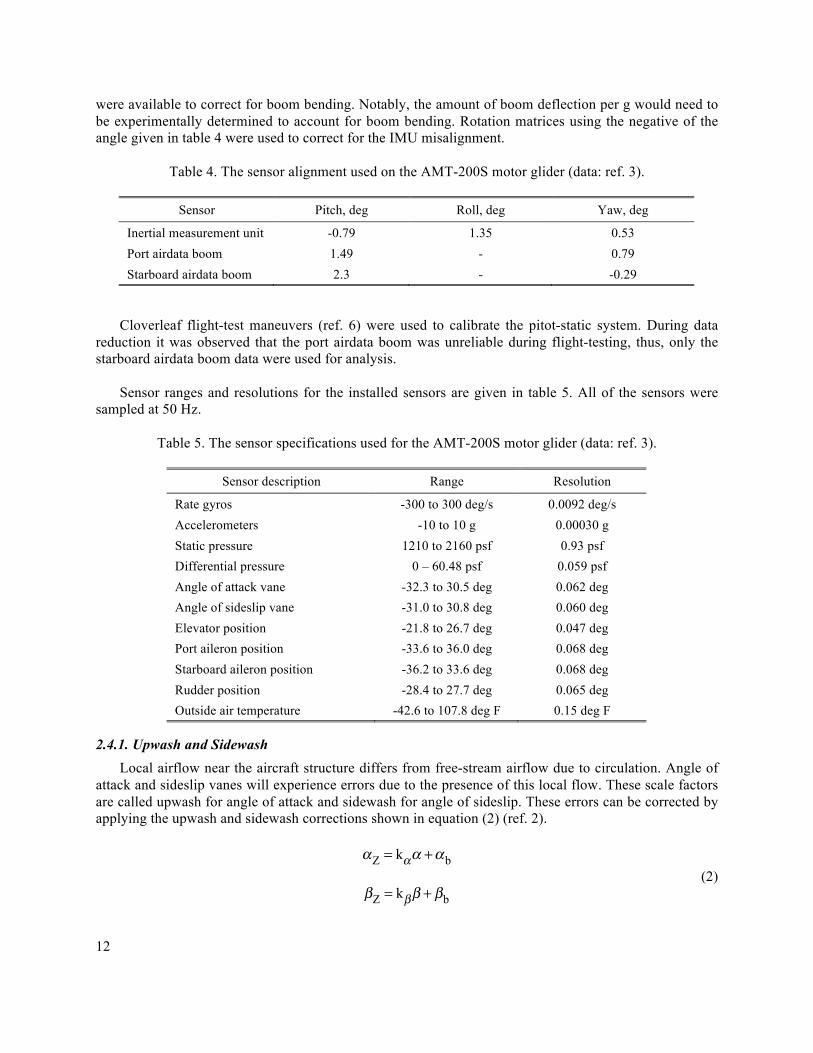
an inclinometer were used to generate alignment corrections; table 4 presents the sensor alignments. To apply the corrections, Haering’s method (ref. 5), was used for the airdata booms. Note that only alignment, flank angle, and installation location were corrected for; insufficient data for the airdata booms

 

 

12

were available to correct for boom bending. Notably, the amount of boom deflection per g would need to be experimentally determined to account for boom bending. Rotation matrices using the negative of the angle given in table 4 were used to correct for the IMU misalignment.

Table 4. The sensor alignment used on the AMT-200S motor glider (data: ref. 3).

Sensor Pitch, deg Roll, deg Yaw, deg

Inertial measurement unit -0.79 1.35 0.53 Port airdata boom 1.49 - 0.79 Starboard airdata boom 2.3 - -0.29

Cloverleaf flight-test maneuvers (ref. 6) were used to calibrate the pitot-static system. During data reduction it was observed that the port airdata boom was unreliable during flight-testing, thus, only the starboard airdata boom data were used for analysis.

Sensor ranges and resolutions for the installed sensors are given in table 5. All of the sensors were sampled at 50 Hz.

Table 5. The sensor specifications used for the AMT-200S motor glider (data: ref. 3).

Sensor description Range Resolution

Rate gyros -300 to 300 deg/s 0.0092 deg/s Accelerometers -10 to 10 g 0.00030 g Static pressure 1210 to 2160 psf 0.93 psf Differential pressure 0 – 60.48 psf 0.059 psf Angle of attack vane -32.3 to 30.5 deg 0.062 deg Angle of sideslip vane -31.0 to 30.8 deg 0.060 deg Elevator position -21.8 to 26.7 deg 0.047 deg Port aileron position -33.6 to 36.0 deg 0.068 deg Starboard aileron position -36.2 to 33.6 deg 0.068 deg Rudder position -28.4 to 27.7 deg 0.065 deg Outside air temperature -42.6 to 107.8 deg F 0.15 deg F

2.4.1. Upwash and Sidewash Local airflow near the aircraft structure differs from free-stream airflow due to circulation. Angle of

attack and sideslip vanes will experience errors due to the presence of this local flow. These scale factors are called upwash for angle of attack and sidewash for angle of sideslip. These errors can be corrected by applying the upwash and sidewash corrections shown in equation (2) (ref. 2).

αZ = kαα +αb

βZ = kββ + βb

(2)

 

 

13

Elements αz and βz are the measured angle of attack and sideslip, kα and

kβ are the upwash and

sidewash, αb and βb are angle of attack and sideslip biases, and α and β are the free-stream angle of attack and sideslip. The upwash and sidewash corrections were obtained during the parameter estimation process.

3. Parameter Estimation Parameter estimation was performed using a time-domain output-error method with non-linear

equations of motion as implemented in pEst (ref. 7). The pEst is a Fortran program for parameter estimation based on Modified Maximum Likelihood Estimator (MMLE) programs used from 1972 to 1990, which themselves were based on parameter estimation programs from as early as 1968 (ref. 8).

3.1. Background

Parameter estimation involves the creation of mathematical models for physical systems from knowledge of the input and response of the system, as depicted in figure 7.

Figure 7. The dynamic response of a system.

As they relate to aircraft, inputs are generally control effectors and responses are sensor measurements. In the case at hand, for longitudinal maneuvers the input is elevator deflection and the responses are angle of attack, pitch rate, normal acceleration, and axial acceleration. For lateral maneuvers the inputs are the ailerons and rudder and the responses are angle of sideslip, roll rate, yaw rate, bank angle, and lateral acceleration.

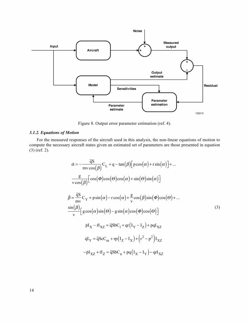
3.1.1. Output-Error Theory Output-error parameter estimation follows the basic flowchart shown in figure 8. Input to the system

produces a measured response from the flight data as well as a computed response from the aircraft model. The parameters of the aircraft model are updated to minimize the difference between measured and computed aircraft response, or residual. Parameter updates are made by determining the sensitivity of computed response to changes in parameter values.

 

 

14

Figure 8. Output error parameter estimation (ref. 4).

3.1.2. Equations of Motion For the measured responses of the aircraft used in this analysis, the non-linear equations of motion to

compute the necessary aircraft states given an estimated set of parameters are those presented in equation (3) (ref. 2).

α = −qS

mv cos β( )CL + q − tan β( ) pcos α( ) + r sin α( )⎡⎣ ⎤⎦ + ...

gv cos β( ) cos Φ( )cos Θ( )cos α( ) + sin Θ( )sin α( )⎡⎣ ⎤⎦

β =qSmv

CY + psin α( )− r cos α( ) + gv

cos β( )sin Φ( )cos Θ( ) + ...

sin β( )v

gcos α( )sin Θ( )− gsin α( )cos Φ( )cos Θ( )⎡⎣ ⎤⎦

pIX − rIXZ = qSbCl + qr IY − IZ( ) + pqIXZ

qIY = qScCm + rp IZ − IX( ) + r2 − p2( ) IXZ

− pIXZ + rIZ = qSbCn + pq IX − IY( )− qrIXZ

(3)

 

 

15

Note that the equations are given for an unpowered aircraft that is symmetric about the X-Z plane. Given arbitrary instrument offsets from the aircraft C.G., the equations to compute the output estimate are as given in equation (4) (ref. 2).

αZ = kα α −

Xαv

q +Yαv

p⎛

⎝⎜

⎞

⎠⎟ +αb

βZ = kβ β −

Zβv

p +Xβv

r⎛

⎝⎜⎜

⎞

⎠⎟⎟+ βb

pZ = p + pb

qZ = q + qb

rZ = r + rb

an =

qSmg

CN +Xan

gq +

Zang

q2 + p2( )− Yangp + anb

ax = −

qSmg

CA +Zaxgq −

Xaxg

q2 + r2( )− Yaxgr + axb

ay =

qSmg

CY −Zay

gp +

Xay

gr −

Yay

gp2 + r2( ) + ayb

(4)

Equation (1) provides a means to convert between normal/axial parameters and lift/drag parameters in

equation (3) and equation (4). Care should be taken when choosing units for the acceleration portion of equation (4). The estimated parameters in the above equations form a Taylor series expansion such as that shown in equation (5).

CN = CN0 +CNαα +C

Nα2α2 +CNq

qc2v

+CNδeδe (5)

The element CN is the total normal force coefficient, CN0 is the trim normal force coefficient, CNα

is the normal force coefficient due to angle of attack, CNq is the normal force coefficient due to pitch

rate, and CNδe is the normal force coefficient due to elevator deflection.

3.1.3. Cramér-Rao Bounds Confidence intervals of the estimated parameters are given by the Cramér-Rao bounds. These bounds

have classically been computed assuming that the variance in the parameter estimates have a normal distribution about the true value. In reality, un-modeled aircraft dynamics cause the variance in parameter

 

 

16

estimates to look like colored noise instead of the white noise generated by a normal distribution. Typically, the actual variance in parameter estimates exceeds the Cramér-Rao bounds by a factor of five to ten. For this analysis, Cramér-Rao bounds were computed using a method presented by Klein and Morelli in reference 9 that takes into account the colored noise in the variance. The Cramér-Rao bounds are indicated on the figures as error bars and the true variance can be seen by the scatter in the results.

3.2. Application

Pitch, roll, and yaw doublets were used to generate the excitations. Doublets were performed with wingtips on and off as well as power-on or power-off. Only power-off data were analyzed due to the unavailability of an accurate engine model. The data were not filtered because noise should not adversely affect parameter estimates and lag could introduce error in control effectiveness estimates. The use of integration with the output-error method tends to smooth out noise in the measured data.

3.2.1. Active Parameters Table 6 contains a list of parameters that were estimated for the AMT-200S motor glider using the

output-error method. Measurement bias for the accelerometers was estimated per the recommendation in section 3.6.2 of reference 2.

Table 6. The estimated parameters determined for use with the AMT-200S motor glider.

Longitudinal Lateral-directional Sensors

CN0 Cm0 CA0 CY0 Cl0 Cn0 kα

CNα Cmα CAα CYβ

Clβ

Cnβ

kβ

C

Nα2 Cmq

C

Aα2 CYp

Clp

Cnp

axb

CNq

Cmδe CAq

CYr Clr Cnr anb

CNδe - CAδe CYδa Clδa Cnδa ayb

- - - CYδ r Clδ r Cnδ r -

3.3. Flight-Test Point Summary

Flight tests were performed by the Project Have MOTO team from 14 March 2008 to 24 March 2008. Longitudinal and lateral-directional doublets were performed with engine power on or off and wingtips on or off. Maneuvers were performed at trimmed airspeeds between 60 kn and 90 kn and at altitudes between 5,000 ft and 10,000 ft MSL. Power-off maneuvers were performed with the engine off and the propeller fully feathered. Table 7 presents a summary of the parameter estimation flights.

 

 

17

Table 7. Data summarizing the AMT-200S motor glider parameter estimation flights.

Date Wingtips Maneuver type Airspeed Altitude, MSL

14 March 2008 Off Longitudinal and lateral 60 kn 5,000-10,000 ft

17 March 2008 On Longitudinal and lateral 60 kn 5,000-10,000 ft

18 March 2008 On Lateral 60 kn 5,000-10,000 ft

19 March 2008 On Longitudinal and lateral 60 kn 5,000-10,000 ft

21 March 2008 Off Longitudinal and lateral 60-80 kn 7,000-10,000 ft

24 March 2008 On Longitudinal and lateral 60-80 kn 5,000-10,000 ft

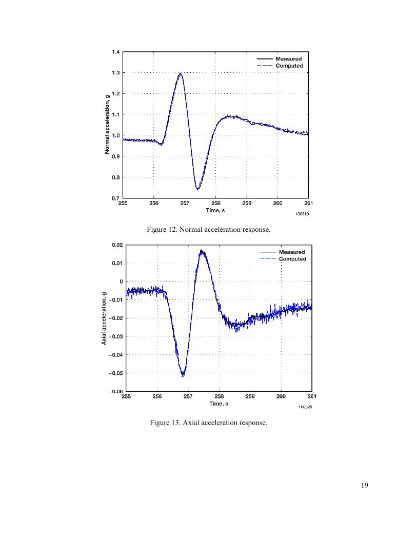
4. Results Parameter estimation quality can be qualitatively evaluated by comparing the measured time history

of the aircraft response with the computed time history of the aircraft response. A typical example of input and responses for a longitudinal maneuver is given in figure 9 through figure 13; a typical example of input and responses for a lateral maneuver is given in figure 14 through figure 18. Aileron and rudder doublets were performed and analyzed separately; only data from an aileron doublet are shown in figure 14 through figure 18.

Figure 9. Longitudinal control surface input.

 

 

18

Figure 10. Angle of attack response.

Figure 11. Pitch rate response.

 

 

19

Figure 12. Normal acceleration response.

Figure 13. Axial acceleration response.

 

 

20

Figure 14. Lateral control surface input.

Figure 15. Angle of sideslip response.

 

 

21

Figure 16. Roll rate response.

Figure 17. Yaw rate response.

 

 

22

Figure 18. Lateral acceleration response.

 

 

23

4.1. Performance

Lift performance and pitching moment of the aircraft were computed from the longitudinal parameters by using the lift and pitching moment equations, shown as equation (6),

CL = CL0 +CLαα +C

Lα2α2

Cm = Cm0 +Cmαα (6)

where α is the aircraft angle of attack. Lift and pitching moment as a function of angle of attack were computed for all doublets, as can be seen in figure 19 and figure 20. Drag was not computed from the longitudinal parameters since it could not be estimated accurately from the doublet maneuvers. The change in drag during a doublet maneuver is relatively small and difficult to measure accurately.

The trim elevator deflection as a function of angle of attack was also computed, as shown in figure 21.

Note that the slope of the pitching moment curves is the static stability of the aircraft. It is also interesting to note that as the pitching moment approaches zero, the elevator trim also approaches zero, as would be expected.

Figure 19. Coefficient of lift.

 

 

24

Figure 20. Pitching moment coefficient.

Figure 21. Trim elevator deflection.

 

 

25

4.2. Analysis of Richard Johnson’s AMT-200 Evaluation

More accurate performance data for the AMT-200 can be found in the Richard Johnson article (ref. 1). In order to provide a complete set of data, it was desirable to analyze and present Johnson’s AMT-200 flight-test data. One difficulty was the definition of angle of attack. Defining the zero angle of attack is completely arbitrary and was not specified for either the Johnson or the Project Have MOTO data sets.

Extrapolation was used to determine the zero lift angle of attack for both sets of data. The difference was found to be -4.25 deg. This correction was applied to all of the performance data derived from Johnson’s data set, presented in figure 23 through figure 26. Figure 22 shows how the lift curve slopes of the two data sets line up with the correction applied. Further validation of the correction can be seen in figure 23 by the good agreement shown in the trim data derived from Johnson’s data set and the Project Have MOTO data set. In addition, as can be seen in figure 25, the angle of attack for the best glide for the AMT-200S motor glider is approximately two and one-half degrees.

Figure 22. Coefficient of lift with Johnson’s data.

 

 

26

Figure 23. Trim speed.

Figure 24. Coefficient of drag, Johnson’s data.

 

 

27

Figure 25. Lift to drag ratio, Johnson’s data.

Figure 26. Sink rate, Johnson's data.

 

 

28

4.3. Longitudinal

Longitudinal parameter estimates and estimated upwash are given in figure 27 through figure 41. The output error parameter estimation was performed with pitch rate and angle of attack as computed states. Responses used were pitch rate, angle of attack, normal acceleration, and axial acceleration. Recommended fairings are included on each figure in this group, indicated by a dashed line to ease implementation of an aerodynamic model of the AMT-200S motor glider. The fairings were calculated by fitting a linear curve to the data. Appendix A contains the equations for each linear curve.

The estimated upwash, figure 27, is significant, ranging from 18 percent to 35 percent. Using angle of attack without taking this into account could lead to potentially significant errors even though the airdata booms extended approximately four feet beyond the leading edge of the wing. The upwash having been estimated, the angle of attack can be corrected using the method presented in equation (2).

Figure 27. Upwash estimate.

Figure 28 through figure 30 depict the trim values of normal and axial force coefficient as well as pitching moment coefficient. Note that trim pitching moment coefficient varies with angle of attack; this behavior indicates that the pitching moment coefficient varies quadratically with angle of attack, as opposed to conforming to the linear model that was assumed.

 

 

29

Figure 28. Trim normal force coefficient.

Figure 29. Trim pitching moment coefficient.

 

 

30

Figure 30. Trim axial force coefficient.

The change in normal force coefficient with angle of attack is related to the lift curve slope by a rotation through angle of attack; refer to equation (1). Note from figure 31 that the normal force coefficient variation with angle of attack agrees with the approximate theoretical value of 0.1097 deg-1 for an elliptical lift distribution. As can be seen in figure 32, Cmα , a measure of the longitudinal static stability of the aircraft, is estimated to be stable and constant with angle of attack.

 

 

31

Figure 31. Normal force coefficient due to angle of attack.

Figure 32. Pitching moment coefficient due to angle of attack.

 

 

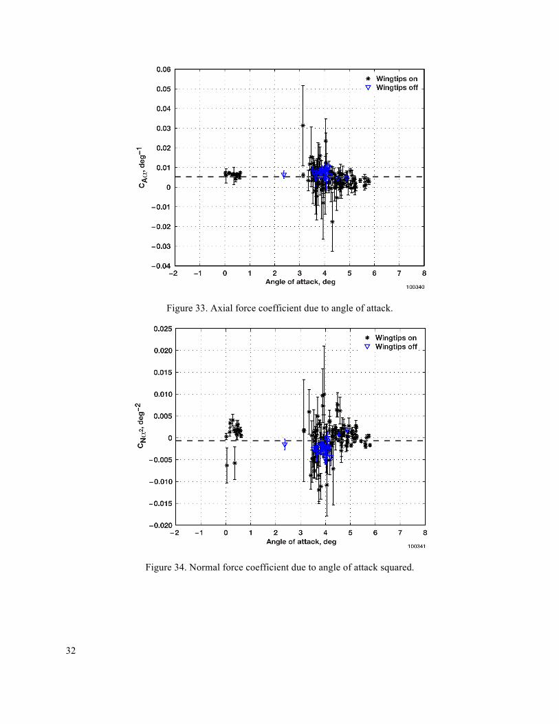
32

Figure 33. Axial force coefficient due to angle of attack.

Figure 34. Normal force coefficient due to angle of attack squared.

 

 

33

Figure 35. Axial force coefficient due to angle of attack squared.

Figure 36. Normal force coefficient due to pitch rate.

Dynamic longitudinal stability of the aircraft is given by the pitch rate damping; see figure 37. This parameter gives the aircraft response to a pitch disturbance. In this case, the aircraft would respond to a pitch-up disturbance by producing a pitch-down moment and the resulting aircraft motion would damp

 

 

34

out over time, which is a stable response. As angle of attack increases, the pitch rate damping becomes slightly less stable, as expected.

Figure 37. Pitching moment coefficient due to pitch rate.

Figure 38. Axial force coefficient due to pitch rate.

Aircraft heaving and elevator control effectiveness are shown in figure 39 and figure 40. Heaving is caused by the momentary increase in normal force as the elevator deflection increases the camber of the

 

 

35

horizontal tail. This effect leads to the aircraft heaving upward slightly before the pitching down. Elevator control effectiveness gives the amount of pitching moment that the elevator is able to produce per degree of control deflection. This result is the control authority of the aircraft.

Figure 39. Normal force coefficient due to elevator deflection.

Figure 40. Pitching moment coefficient due to elevator deflection.

 

 

36

Figure 41. Axial force coefficient due to elevator deflection.

 

 

37

4.4. Lateral-Directional

Lateral-directional parameter estimates and estimated sidewash are given in figure 42 through figure 59. The output error parameter estimation was performed with sideslip, roll rate, yaw rate, and bank angle as computed states. Responses used were sideslip, roll rate, yaw rate, bank angle, and lateral acceleration. Recommended fairings are included on the figures as indicated by the dashed line to ease implementation of an aerodynamic model of the AMT-200S motor glider.

Sidewash correction, shown in figure 42, is estimated to decrease from 7 percent to 4 percent over the angle-of-attack range tested. In this case, sidewash would be due to flow off the fuselage and any crossflow over the wing. Angle of sideslip can now be corrected using the method presented in equation (2).

Figure 42. Sidewash estimate.

 

 

38

Figure 43. Trim lateral force coefficient.

Figure 44. Trim rolling moment coefficient.

 

 

39

Figure 45. Trim yawing moment coefficient.

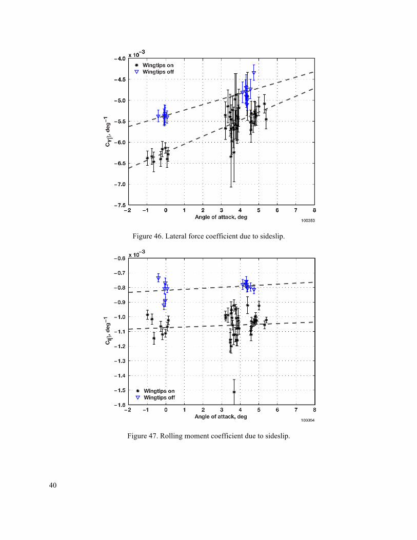
Lateral force coefficient and rolling moment coefficient due to sideslip was higher for the aircraft configuration with wingtips on than wingtips off, as seen in figure 46 and figure 47. This result is likely due to the increased vertical surface area above the C.G. from the wingtips. Yawing moment coefficient due to sideslip is the weathervaning tendency of the aircraft. In this case it is stable and decreases slightly with angle of attack.

 

 

40

Figure 46. Lateral force coefficient due to sideslip.

Figure 47. Rolling moment coefficient due to sideslip.

 

 

41

Figure 48. Yawing moment coefficient due to sideslip.

Rolling moment coefficient due to roll rate, shown in figure 49, gives the dynamic stability of the aircraft in the roll axis. In this case it is stable and approximately constant with angle of attack.

Figure 49. Rolling moment coefficient due to roll rate.

 

 

42

Figure 50. Yawing moment coefficient due to roll rate.

Figure 51. Lateral force coefficient due to roll rate.

Rolling moment coefficient due to yaw rate is generated by the difference in airspeed over the left and right wing halves, as shown in figure 52. As the aircraft experiences positive yaw rate the left wing will experience a slightly higher airspeed, and hence lift, than the right wing. This difference in lift will cause the aircraft to roll. Additionally, side force from the vertical tail due to yaw rate and sideslip will cause the aircraft to roll due to its position above the aircraft C.G..

 

 

43

Yawing moment coefficient due to yaw rate is the dynamic stability of the aircraft in the yaw axis,

shown in figure 53. In this case it is stable and approximately constant with angle of attack.

Figure 52. Rolling moment coefficient due to yaw rate.

Figure 53. Yawing moment coefficient due to yaw rate.

 

 

44

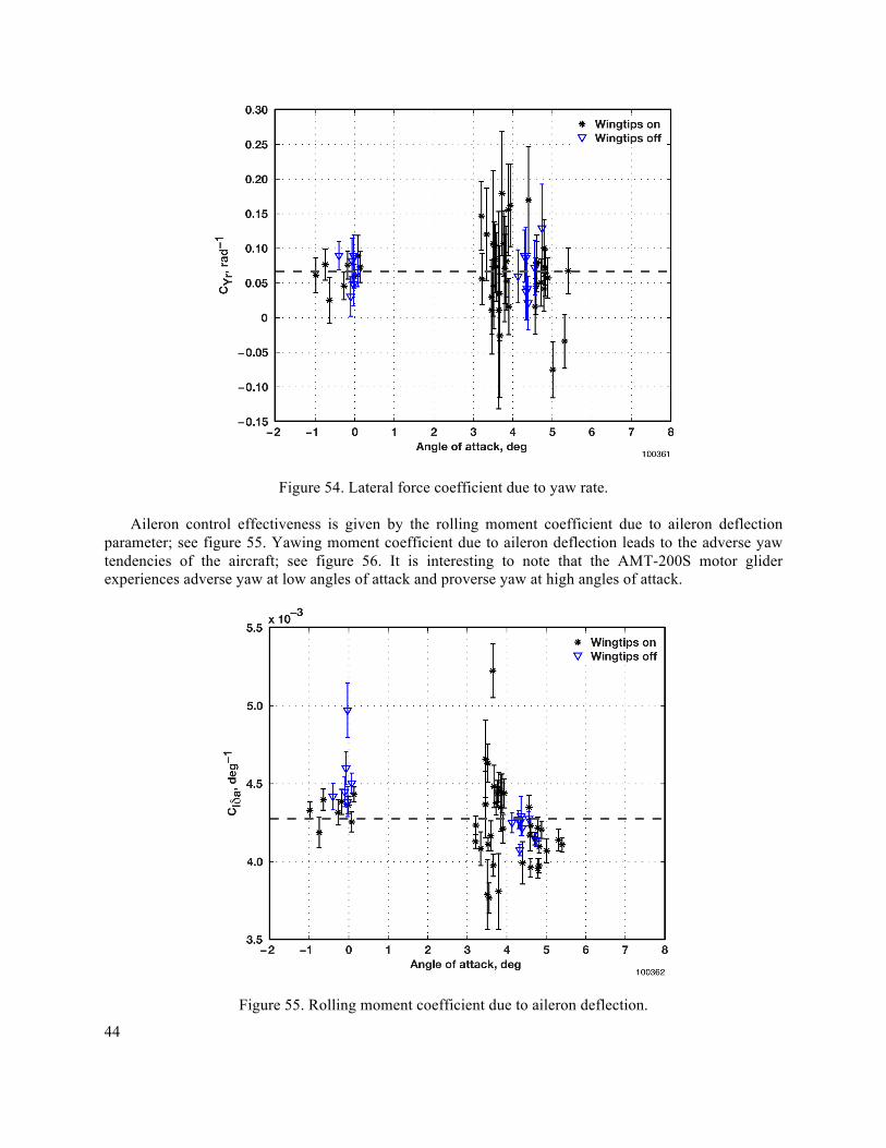
Figure 54. Lateral force coefficient due to yaw rate.

Aileron control effectiveness is given by the rolling moment coefficient due to aileron deflection parameter; see figure 55. Yawing moment coefficient due to aileron deflection leads to the adverse yaw tendencies of the aircraft; see figure 56. It is interesting to note that the AMT-200S motor glider experiences adverse yaw at low angles of attack and proverse yaw at high angles of attack.

Figure 55. Rolling moment coefficient due to aileron deflection.

 

 

45

Figure 56. Yawing moment coefficient due to aileron deflection.

Figure 57. Lateral force coefficient due to aileron deflection.

Rolling moment coefficient due to rudder deflection is caused by the side force of the rudder located above the aircraft C.G.; see figure 58.

 

 

46

Figure 58. Rolling moment coefficient due to rudder deflection.

Control effectiveness of the rudder is given in figure 59. In this case it is approximately constant over the angle-of-attack range tested. Lateral force due to rudder deflection is caused directly by the deflection of the control surface, as shown in figure 60.

 

 

47

Figure 59. Yawing moment coefficient due to rudder deflection.

Figure 60. Lateral force coefficient due to rudder deflection.

 

 

48

5. Conclusions and Future Research Output-error parameter estimation seemed to produce reasonable performance and parameter

estimates for the subject motor glider. A few interesting observations can be made from the results: first, upwash was significant and is a factor that should be accounted for in future flight-test or parameter estimation efforts; second, the only noticeable effect of the wingtip extensions was an increase in side force and rolling moment due to sideslip. The team concludes that the parameter and performance estimates presented, along with the data from previous well-known flight tests, should enable the creation of a motor glider simulation.

 

 

49

Appendix A Linear Curve Equations

Equations given in the table below are in the form Y = AX + B.

Parameter Figure A B

Trim elevator deflection 21 2.6137030208 -0.4533717581

CN0 28 0 0.4541620945

CNα 31 0 0.1007619850

C

Nα2 34 0 -0.0006171816

CNq 36 0 7.6107312451

CNδe 39 0 0.0052123049

Cm0 29 0.0620335317 -0.0018978809

Cmα 32 0 -0.0107407416

Cmq 37 -32.2942895315 1.2107406516

Cmδe 40 0 -0.0241452667

CA0 30 0 0.0589883048

CAα 33 0 0.0052287626

C

Aα2 35 0 0.0016590893

CAq 38 0 2.6838326559

CAδe 41 0 0.0034553188

kα 27 1.3122514321 -0.0163824724

CY0 43 0.0085890739 0.0022272756

CYβ wingtips on 46 -0.0062384300 0.0001910126

CYβ wingtips off 46 -0.0053630910 0.0001309538

CYp 51 0.3106500839 -0.0188294869

 

 

50

Parameter (cont.) Figure (cont.) A (cont.) B (cont.)

CYr 54 0 0.0668160855

CYδa 57 -0.0024421825 0.0001333706

CYδ r 60 0.0020231848 0.0000498082

Cl0 44 0 -0.0040903491

Clβ wingtips on 47 -0.0010739081 0.0000046861

Clβ wingtips off 47 -0.00081888534 0.0000069324

Clp 49 0 -0.5343131014

Clr 52 0.1050098235 0.0066916046

Clδa 55 0 0.0042754248

Clδ r 58 0.0001605999 -0.0000131488

Cn0 wingtips on 45 0 0.0011115962

Cn0 wingtips off 45 0 0.0015987246

Cnβ 48 0.0009312555 -0.0000301560

Cnp 50 -0.0215391697 -0.0144784563

Cnr 53 0 -0.0276735756

Cnδa 56 -0.00001716527 0.0000557239

Cndr 59 0 -0.0005558636

kβ 42 1.0694654047 -0.0060865973

 

 

51

References 1. Johnson, Richard H., “A Flight Test Evaluation of the Super Ximango Motorglider,” Soaring,

December 1996, pp. 35-40.

2. Maine, Richard E., and Kenneth W. Iliff, Application of Parameter Estimation to Aircraft Stability and Control, The Output-Error Approach, NASA Reference Publication 1168, 1986.

3. Leigh, Elliot J., Devin S. Traynor, Gyandeep Singh, Rotem Maril, and Michael J. Marlin,

“TG-14A Parameter Identification (Project Have MOTO),” AFFTC-TIM-08-06, 2008.

4. Cloud Cap Technology: http://www.cloudcaptech.com/default.shtm. Accessed January 28, 2011.

5. Haering, Edward A., Jr., Airdata Calibration of a High-Performance Aircraft for Measuring Atmospheric Wind Profiles, NASA TM-101714, 1990.

6. Olson, Wayne M. “Pitot-Static Calibrations Using a GPS Multi-Track Method,” presented at the

SFTE Symposium, Reno, Nevada, September 1998.

7. Maine, Richard E., “pEst – Parameter Estimation (Version 4.0 with modifications),” computer software.

8. Maine, Richard E., User’s Manual for pEst Version 3.0, 2003.

9. Klein, Vladislav, and Eugene A. Morelli, Aircraft System Identification Theory and Practice,

American Institute of Aeronautics and Astronautics, Inc., Reston, Virginia, 2006.