Ambipolar Drift Heating in Turbulent Molecular Clouds

Paolo Padoan

Harvard University Department of Astronomy, Cambridge, MA 02138,

padoan@cfa.harvard.edu

Ellen Zweibel

JILA, University of Colorado at Boulder, Boulder CO 80309-440,

zweibel@solarz.colorado.edu

Ake Nordlund

Astronomical Observatory and Theoretical Astrophysics Center, Juliane Maries Vej 30,

DK-2100 Copenhagen, Denmark, aake@astro.ku.dk

Received ; accepted

– 2 –

ABSTRACT

Although thermal pressure is unimportant dynamically in most molecular

gas, the temperature is an important diagnostic of dynamical processes and

physical conditions. This is the first of two papers on thermal equilibrium in

molecular clouds. We present calculations of frictional heating by ion-neutral

(or ambipolar) drift in three–dimensional simulations of turbulent, magnetized

molecular clouds.

We show that ambipolar drift heating is a strong function of position in

a turbulent cloud, and its average value can be significantly larger than the

average cosmic ray heating rate. The volume averaged heating rate per unit

volume due to ambipolar drift, HAD = |J×B|2/ρiνin ∼ B4/(16π2L2Bρiνin), is

found to depend on the rms Alfvenic Mach number, MA, and on the average

field strength, as HAD ∝ M2A〈|B|〉4. This implies that the typical scale of

variation of the magnetic field, LB, is inversely proportional to MA, which we

also demonstrate.

– 3 –

1. Introduction

Observations reveal that roughly 20% - 40% of the interstellar gas in the Galactic

disk is organized into Giant Molecular Clouds (GMCs). These clouds appear to be self

gravitating and roughly in virial equilibrium. The density distribution in the clouds is

highly inhomogeneous, and the velocity field is turbulent and highly supersonic. It is

thought that both magnetic and turbulent kinetic pressure contribute to cloud support, but

the relative degree of magnetic support is uncertain because of the observational difficulty

of measuring the magnetic field strength and topology.

Several lines of evidence suggest that GMCs survive for a few tens of millions of

years, but both analytical estimates, some dating back more than two decades (Goldreich

& Kwan 1974, Field 1978, Zweibel & Josafatsson 1983, Elmegreen 1985), and numerical

simulations (Scalo & Pumphrey 1982, Stone, Ostriker, & Gammie 1998, MacLow 1999,

Padoan & Nordlund 1999) suggest that molecular cloud turbulence dissipates in much

less than the cloud lifetime. Star formation is observed to take place in nearly all GMCs,

and it appears that the lifetimes of GMCs are determined by the rate at which they are

destroyed by energy and momentum input from the massive stars which form within them.

It also appears likely that energy input from stars, and possibly from other sources, drives

turbulence in GMCs as well.

Ambipolar drift, or ion-neutral friction, has long been thought to be an important

energy dissipation mechanism in molecular clouds, and therefore a significant heating

mechanism for molecular cloud gas (Scalo 1977, Goldsmith & Langer 1978, Zweibel &

Josafatsson 1983, Elmegreen 1985). In fact, as first suggested by Scalo (1977), the observed

low temperatures of molecular clouds places upper limits on the rate of energy dissipation

by ambipolar drift, and thus, with some additional assumptions, on the magnetic field

strength.

– 4 –

Nevertheless, it has been difficult to assess the rate of energy dissipation by ambipolar

drift. The frictional heating rate HAD depends on the local Lorentz force in the medium,

which is almost impossible to measure. Simple scaling arguments show that HAD is

proportional to B4n−1n−1i L−2

B , where B, n, ni, and LB are the magnetic field strength,

neutral density, ion density, and magnetic length scale, respectively. The extreme sensitivity

of this formula to magnetic field strength, only the line of sight average value of which

can be directly measured, and to the essentially unobservable LB, has made it difficult to

estimate HAD with confidence even to order of magnitude.

In this paper, we use numerical simulations of magnetized turbulence to study heating

by ambipolar drift in molecular clouds. We show that the ambipolar heating rate per unit

volume, HAD, depends on field strength as B4, for constant rms Mach number of the flow,

and on the Alfvenic Mach number as M2A. This implies that the magnetic length scale,

LB, depends on the Alfvenic Mach number as M−1A , which we demonstrate. We show

that the numerical value of the heating rate, computed by solving the three–dimensional

compressible magneto–hydrodynamic (MHD) equations, tends to converge with increasing

numerical resolution, and therefore we can fully quantify the value of HAD, to within an

uncertainty of less than a factor of two, in the numerical models.

These empirical formulae make it much easier to estimate ambipolar drift heating in

terms of observable properties of clouds. The average heating rate depends on B2, rather

than B4 as in the traditional expression, on the line width or rms velocity, and on the

neutral and ion densities. The magnetic length scale is eliminated through its dependence

on MA.

We find that ambipolar drift is probably a stronger heating mechanism than cosmic

ray heating, and that it is a strong damping mechanism for molecular cloud turbulence,

leading to significant decay within one dynamical crossing time.

– 5 –

In §2 of the paper we briefly summarize the physics of ambipolar drift heating, and in

§3 we describe the simulations. In §4 we present results of the computation of ambipolar

drift heating rate, and in §5 we discuss some implications of the results and summarize the

conclusions of this work.

2. Dynamics and Dissipation of Weakly Ionized Gas

Molecular cloud gas includes neutral atoms and molecules, atomic and molecular ions,

electrons, and dust grains, which may also be electrically charged. At the gas densities

considered in this paper (0.1 cm−3 < n < 105 cm−3, and 〈n〉 = 320 cm−3), electrons are

the primary current carriers, the number density of ions much exceeds the number density

of grains, and Ohmic dissipation is negligible (Nakano & Umebayashi 1986). Moreover,

significant charge separation cannot be sustained on the time scales and length scales of

interest, so the electrons and ions move together. The electric field is then given by

E = −vi

c×B, (1)

where vi is the velocity of the ion, or plasma component.

In principle, vi and the neutral velocity vn should be determined by solving separate

fluid equations for these species (Draine 1986), including their coupling by collisional

processes. In typical molecular cloud environments this leads to a great disparity of

length scales and time scales, because ions collide with neutrals at a very high frequency

compared to other rates in the problem. Past computations of two fluid systems (Toth

1994, Brandenburg & Zweibel 1995, Hawley & Stone 1998) have avoided this problem by

assuming ion to neutral density ratios that are far higher than the values found in typical

– 6 –

molecular clouds. An alternative, which we pursue here, is to consider only the length scales

and time scales over which the ions and neutrals are well coupled (Shu 1983).

We introduce the drift velocity vD

vD ≡ vi − vn (2)

and evaluate vD by assuming that the dominant forces on the charged component are the

Lorentz force and the frictional force arising from collisions with neutrals. We model the

latter in the standard way as

Fin = −ρiνinvD, (3)

where ρiνin = ρnνni = ρiρn〈σv〉/(mi + mn). In numerical work, we will take the collision

rate coefficient 〈σv〉 = 2× 10−9 cm3/s (Draine, Roberge, & Dalgarno 1983) and assume the

ions are HCO+ (cf. de Jong, Dalgarno, & Boland 1980) and the neutrals are H2 and He,

with n(He)/n(H2) = 2/9. On time scales longer than the neutral-ion collision time 1/νni,

the Lorentz and drag forces must balance. This leads to an expression for the drift velocity

vD =J×B

cρiνin

. (4)

Making the further assumption ρi/ρ � 1, so that vn is the same as the center of mass

velocity v, the magnetic induction equation is

∂B

∂t= ∇× (vi ×B) = ∇× (v ×B) +∇× (J×B)×B

cρiνin

. (5)

– 7 –

The frictional heating rate HAD is

HAD = ρiνin | vD |2 . (6)

Equations (4), (5), and (6) constitute the strong coupling approximation to ambipolar

drift. They are much easier to solve, and at less computational expense, than the full

two fluid equations that hold for even a single neutral species and a single charged fluid.

Nevertheless, we must consider where these equations break down. The validity of the

strong coupling approximation, even at low drift velocities, can be assessed by evaluating

the ambipolar Reynolds number RAD (Zweibel & Brandenburg 1997)

RAD ≡ LBvνni

v2A

∼ v

vD, (7)

where LB is the length scale on which the magnetic field varies, and in the second relation

we have used eqn. (4). The strong coupling approximation should be valid for RAD ∼> 1.

As examples, this criterion gives the wavenumber for critical damping of small amplitude

MHD waves of wavelength λ if we replace v by vA and LB by λ/π in eqn. (7) (McKee et

al. 1993). And, the criterion for significant ion-neutral separation in shocks (Mullan 1971,

Draine 1980) is equivalent to the condition RAD < 1 evaluated upstream.

We show in §4 that LB ∝ M−1A , where MA is an appropriately averaged Alfven Mach

number defined in eqn. (24). Therefore, RAD ∝ MA: we expect that, on average, the

strong coupling approximation is increasingly good as MA increases. For example, in our

N = 1283 simulations, the value of RAD spans a range from about 5 to about 300, for

0.5 ≤ MA ≤ 30. In practice, however, LB is bounded below by the resolution of the grid,

leading to a flattening of the LB vs MA relation as MA increases. This can be seen in

– 8 –

Figure 3 for MA ∼> 10. Thus, although we do not accurately model MHD shocks in which

two fluid effects are significant (see Draine & McKee 1993), we do resolve much of the

magnetic field structures outside of shocks, at least in simulations with MA < 10.

3. The Simulations

The code and basic equations it solves have been previously described in Nordlund,

Stein & Galsgaard (1996), Nordlund & Galsgaard (1997), Padoan et al. (1998), and Padoan

& Nordlund (1999). Here, we include ambipolar drift, in the strong coupling approximation

described in §2, for the first time, but this has not required changes in the numerical

method.

The code solves the compressible MHD equations on a 3–dimensional staggered mesh,

with volume centered mass density and thermal energy, face centered velocity and magnetic

field components, and edge centered electric currents and electric fields (Nordlund, Stein &

Galsgaard 1996):

∂ ln ρ

∂t+ v · ∇ ln ρ = −∇ · v, (8)

∂v

∂t+ v · ∇v = −P

ρ∇ lnP +

1

cρJ×B + f , (9)

P = ρT, (10)

∂B

∂t= ∇× (v ×B) +∇× (J×B)×B

cρiνin. (11)

– 9 –

4π

cJ = ∇×B, (12)

plus numerical diffusion terms, and with periodic boundary conditions. The system is forced

by f , an external random driver, and all the other symbols have their usual meanings.

In calculating the dynamics we use an isothermal equation of state, as in our previous

work, even though in this paper and the next we are concerned with the thermal equilibrium

of the gas, and preliminary results suggest a significant spread of temperatures. As long

as the motions remain highly supersonic, the dynamics should be almost insensitive to

the thermal pressure, although the equation of state certainly affects the density contrast

produced in shocks.

We use spatial derivatives accurate to 6th order, interpolation accurate to 5th order,

and Hyman’s 3rd order time stepping method (Hyman 1979). The code uses shock and

current sheet capturing techniques to ensure that magnetic and viscous dissipation at the

smallest resolved scales provide the necessary dissipation paths for magnetic and kinetic

energy. As shown by Galsgaard & Nordlund (1996, 1997), dissipation of magnetic energy

in highly turbulent, compressible MHD plasmas occurs at a rate that is independent

of the details of the small scale dissipation. In ordinary hydrodynamic turbulence the

corresponding property is one of the cornerstones of Kolmogorov (1941) scaling.

The initial random velocity field is generated in Fourier space, with a normal

distribution of amplitudes and random phases, and with power only in the Fourier

components in the shell of wave–number 1 ≤ kL/2π ≤ 2. In all but one of the experiments

the flow is driven by an external random force (f in the momentum equation (9)). The

random force is also generated in Fourier space with a normal distribution, with power only

in the range of wave–number 1 ≤ kL/2π ≤ 2. A Helmholtz decomposition is performed on

both the initial velocity and the random force, and only the solenoidal component is used.

– 10 –

In order to produce a force that varies continuously in time, we actually specify randomly

distributed Fourier components of the time derivative of the acceleration, and compute

the acceleration as a time integral. The time derivative of the Fourier components of the

acceleration are regenerated at time intervals of about one dynamical time.

All our models have periodic boundary conditions. This is an efficient way to study the

evolution of MHD turbulence under internal forces, but it precludes study of the coupling

between molecular clouds and the surrounding diffuse medium, such as, for example,

outward radiation of cloud energy in the form of MHD disturbances (Elmegreen 1985).

Since we do not have a physically motivated model for the initial conditions, we allow the

models to relax before studying their statistical properties, and report only results for the

steady state.

For the purpose of computing the ambipolar drift heating rate, we have run several

experiments with external random driving, at an approximately constant sonic rms Mach

number, M ≈ 10, with different values of the magnetic field strength, in a 1283 numerical

grid (named A1 to A7 in Table 1), and a decaying experiment (no external driving), with

approximately constant value of the rms Alfvenic Mach number, MA ≈ 1, and magnetic

field strength that decreases with time (named B1 in Table 1). In order to perform a

convergence study, we have repeated a 1283 experiment at lower resolutions: 643, 323,

and 163 (experiments A4 in Table 1). Finally, we have repeated a 1283 experiment with

different values of the ambipolar drift parameter a, introduced below (experiments A3 in

Table 1). The results of these experiments are presented in the next section, and some

of their parameters are listed in Table 1. When we rescale the experiments to physical

units (see below) we use an average gas density 〈n〉 = 320 cm−3, according to the Larson

relations (Larson 1981; Solomon et al. 1987) and to M ≈ 10. Although ionization by UV

photons is generally important at this relatively low density (and likely low extinction), we

– 11 –

assume in the following that the gas is ionized by cosmic rays. We do so because, while

the volume averaged gas density is relatively low, most of the gas is actually at densities

larger than ten times the mean density, due to the very intermittent density distribution

(Padoan et al. 1998; Padoan & Nordlund 1999). In numerical experiments with M ≈ 10

and numerical mesh size of 1283, the complex system of interacting shocks generates a

very large density contrast of almost six orders of magnitude (0.1 cm−3 ∼< n ∼< 105 cm−3).

However, the ambipolar drift heating rate computed in this work and expressed in eqn. (25)

can be rescaled to any value of the average gas density, and it is increasingly accurate for

increasing average density, because of the assumption of cosmic ray ionization.

Cosmic rays ionization results in the following expression for the fractional ionization

xi:

xi ≡ Ki

n1/2n

(13)

where nn is the number density of neutrals, and Ki is of order 10−5 cm−3/2 (see the

discussion of Ki in McKee et al. 1993). We have not included photoionization by the

ambient radiation field, although it is important at low extinction (McKee 1989). Equation

(13) underestimates the ionization, and hence overestimates the degree of ambipolar drift,

in the low density gas, but our main interest is in the high density regions, which contain

most of the mass.

In order to explain our parameterization of ambipolar drift, we must introduce our

natural units and nondimensionalized equations. We denote quantities defining a unit by a

subscript u and dimensionless quantities by tildes, that is B = B/Bu, v = v/vu, J = ∇× B,

∇ = Lu∇, and n = n/nu . The code is written so that the units are:

Bu = cS(4π〈ρ〉)1/2 (14)

– 12 –

vu = cS (15)

nu = 〈n〉 (16)

Lu = L/N (17)

where cS is the sound speed, L the physical size of the simulation box, and N the linear

resolution of the numerical box.

The ambipolar drift velocity is written as

vD = an−3/2J× B (18)

The ambipolar drift parameter a can be computed from the expression vD = vD/vu,

and using equation (4) and (18), together with (14), (15),(16) and (17). The result is:

a = 0.28(

T

10K

)1/2 ( N

128

)(L

10 pc

)−1 ( 〈n〉200 cm−3

)−1/2 (Ki

10−5 cm−3/2

)−1 ( < σv >

2× 10−9 cm3 s−1

)−1

.

(19)

The value of the parameter a that we use in most of the present experiments is a = 0.3

in 1283 runs, and appropriately rescaled for different resolutions. Using equation (19),

a = 0.3 corresponds to physical conditions in typical molecular clouds with temperature

T = 10 K, size L = 10 pc, and volume averaged number density 〈n〉 = 200 cm−3. Using

Larson’s relation between size and density (Larson 1981; Solomon et al 1987), 〈n〉 ∝ L−1,

the dependence of a on the cloud size would be a ∝ L−1/2. As an example, a cloud or

cloud core with L = 1 pc and 〈n〉 = 2000 cm−3, would require a value of a = 0.88, while a

– 13 –

giant molecular cloud complex with L = 50 pc should be modeled with a = 0.12. Physical

conditions in molecular clouds with sizes in the range 1–50 pc can therefore be reproduced

numerically with values of a within a factor of less than 3 from the value a = 0.3 (at

N = 1283 resolution) adopted in most of the numerical experiments used in this work.

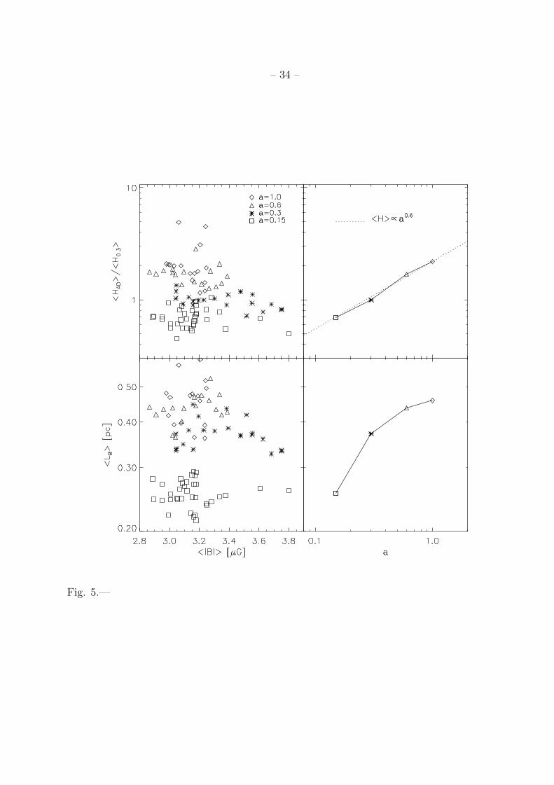
However, the dependence of the ambipolar drift heating rate on the parameter a has

been computed (see Figure 5), by varying the value of a in the simulations in the range

0.15 ≤ a ≤ 1.0, that corresponds to cloud size 0.5 pc∼< L ∼< 50 pc.

4. The Ambipolar Drift Heating Rate

Our results are based on a variety of both driven and decaying cloud models, over a

range of parameters and at different resolutions, as described in the previous section. The

heating rates that we report in the driven models all apply to the steady state, which is

reached after approximately 3-4 dynamical times. However, because all quantities fluctuate

slightly with time with respect to their steady state values, we typically enter values from

several adjacent time slices of each simulation on the figures which follow.

Although, as we show later in this section, the heating rate varies considerably from

point to point, the volume averaged heating rate 〈HAD〉 scales with the properties of the

system in a remarkably simple way. We define the mean of a quantity Q, 〈Q〉, by

〈Q〉 ≡ N−1∑ijk

Qijk, (20)

where ijk indexes a grid point. From eqn. (6),

〈HAD〉 = N−1∑ijk

(ρiνin | vD |2)ijk, (21)

where vD is computed from eqn. (4).

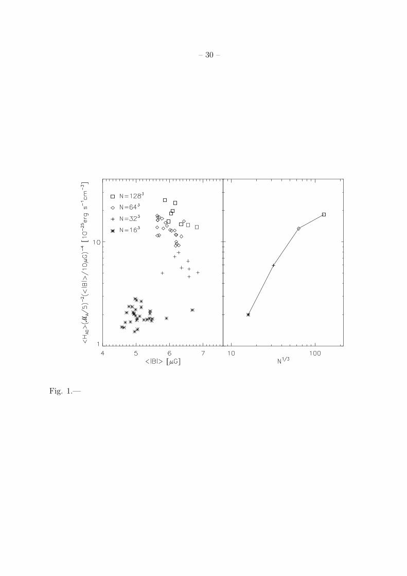
We have performed a convergence study of the dependence of 〈HAD〉 on numerical

resolution. Figure 1 shows 〈HAD〉 for four simulations with N = 163, 323, 643, and 1283,

– 14 –

and shows clear evidence for convergence, probably to better than a factor of 2, of the value

found for the highest resolution.

Studies at high spatial resolution have shown that ambipolar drift can steepen the

current density profile to the point that it virtually becomes singular (Brandenburg &

Zweibel 1994, 1995, Mac Low et al 1995, Zweibel & Brandenburg 1997, Mac Low & Smith

1997). However, the contribution of such structures to the total heating rate is small, as

shown by the following argument. The magnetic field varies with position x across a sheet

as B ∼ x1/3, so J varies as x−2/3. From eqns. (4) and (6), HAD ∝ x−2/3, which is singular,

but integrable: the integrated value of HAD depends on the width xs of the sheet as x1/3s .

Therefore, these very thin structures contribute little to the heating rate - even less if one

takes into account two fluid effects, which resolve the singularity.

Assuming that the heating rate is nearly converged, the scaling law we find for 〈HAD〉depends on the mean magnetic field magnitude 〈| B |〉

〈| B |〉 ≡ 〈(B2)1/2〉, (22)

the rms velocity vrms

vrms ≡ 〈v2〉1/2, (23)

and the Alfven Mach number in the evolved state

MA ≡ vrms(4π〈ρ〉)1/2

〈| B |〉 . (24)

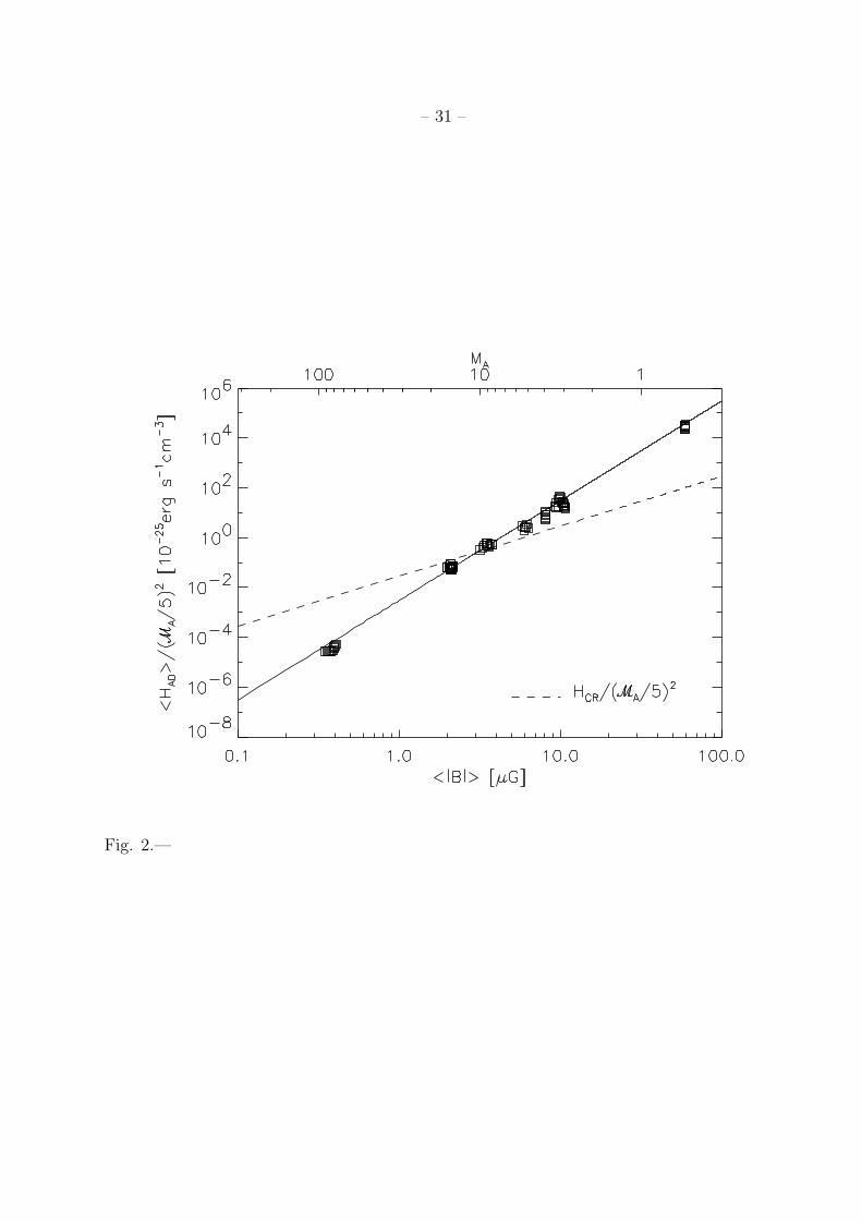
Figure 2 shows 〈HAD〉/M2A plotted versus 〈| B |〉 for a set of simulations with constant sonic

Mach number M = 10. Thus, MA ∝ 〈| B |〉−1 with a unique constant of proportionality, so

we plot MA on the top axis of the figure. In all of these runs, the ambipolar drift parameter

a defined in eqn. (19) is fixed at 0.3 for N = 1283. According to the Larson relations, this

model corresponds to a cloud with L ∼ 6 pc, 〈n〉 ∼ 320 cm−3.

– 15 –

Figure 2 shows a remarkably tight correlation between 〈| B |〉 and 〈HAD〉. The

simulations are fit by the relation

〈HAD〉 = 3.0× 10−24

(〈| B |〉10µG

)4(MA

5

)2( 〈n〉320cm−3

)−3/2

erg cm−3 s−1, (25)

which is shown as a solid line on Figure 2.

The cosmic ray heating rate Hcr corresponding to a primary cosmic ray ionization rate

ζ = 10−17 s−1 is also plotted in Figure 2. Ambipolar drift heating exceeds cosmic ray heating

unless the magnetic field is less than about 3 µ G. However, the value 〈n〉 = 320 cm−3

has been used in Figure 2; for increasing values of the average gas density, the cosmic ray

heating rate increases, since it is proportional to the gas density. The cosmic ray heating

rate is also found to vary considerably from cloud to cloud, and could span the range of

values 10−16 s−1 ∼< ζ ∼< 10−18 s−1 (Caselli et al. 1998; Williams et al. 1998).

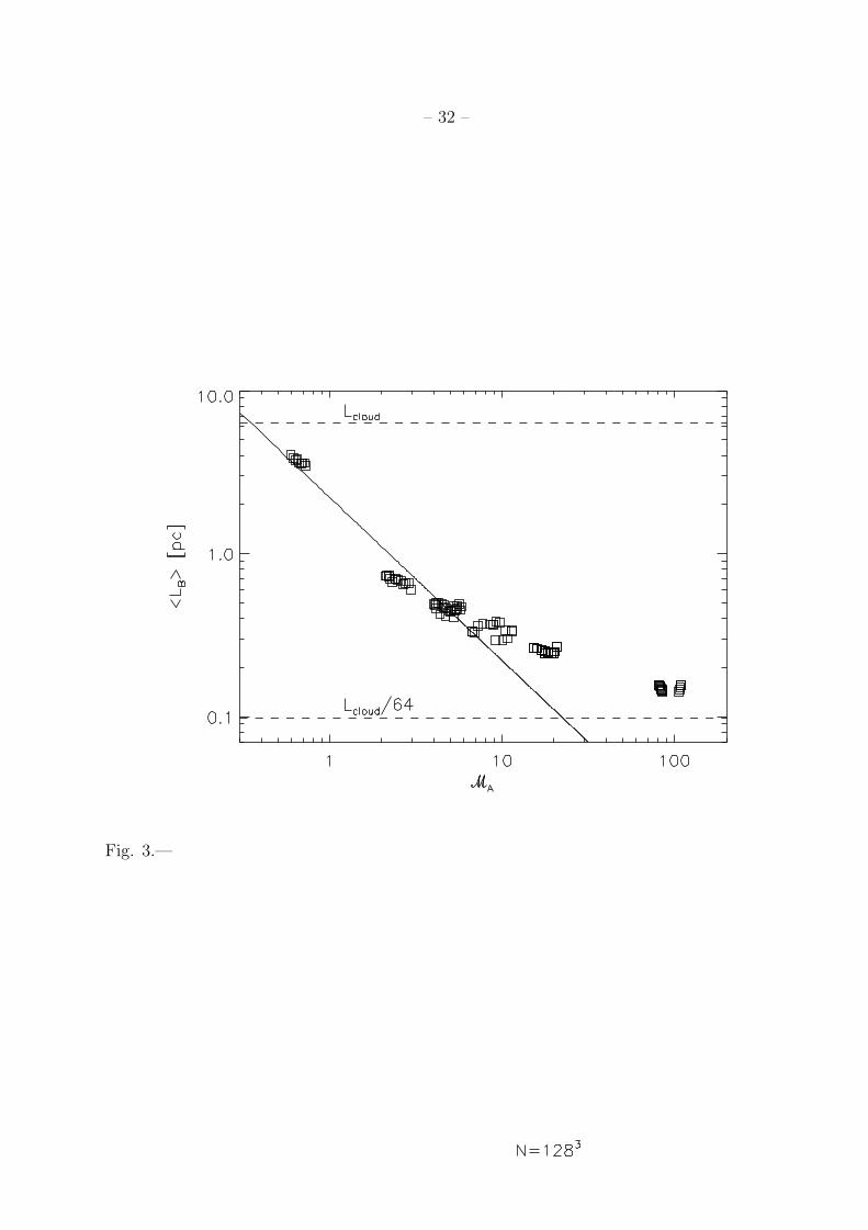
Equation (6) is only compatible with eqn. (25) if

〈LB〉 ≡ 〈(

c2B2

(4πJ)2

)1/2

〉 ∝ M−1A . (26)

Figure 3 shows that this is in fact the case, unless MA > 10. For MA > 10, although

the value of the volume averaged magnetic length scale, 〈LB〉, is still a bit larger than

the numerical grid scale, local values of LB are so small that in many locations LB is not

resolved by the 1283 numerical mesh. It is possible that 〈LB〉 ∝ M−1A also for MA > 10,

but this cannot be shown in numerical runs with the present resolution.

Qualitatively, it is not surprising that 〈LB〉 decreases with increasing MA, or

increasingly dominant kinetic energy. The larger MA is, the more the flow can bend the

field, leading to more tangling and smaller LB. What perhaps is surprising is that in cases

in which the field is initially weak, it is not amplified up to equipartition: if it were, there

would be no points in Figure 3 with MA > 1. A number of factors can lead to saturation of

the field below equipartition. The weaker the field is initially, the more it must be stretched

– 16 –

and tangled to amplify it up to equipartition. The more tangled the field becomes, the more

subject it is to numerical and ambipolar diffusion. It has also been shown (Brandenburg

& Zweibel 1994, Brandenburg et al 1995, Zweibel & Brandenburg 1997) that ambipolar

drift drives the magnetic field to a nearly force free state. Since the flow cannot do work

on a force free field, amplification ceases once the force free state is reached. And finally,

the magnetic field becomes quite spatially intermittent (see Figure 7), and locally strong

Lorentz forces might feed back on the flow and quench the growth of the field even before

ambipolar drift has had enough time to act.

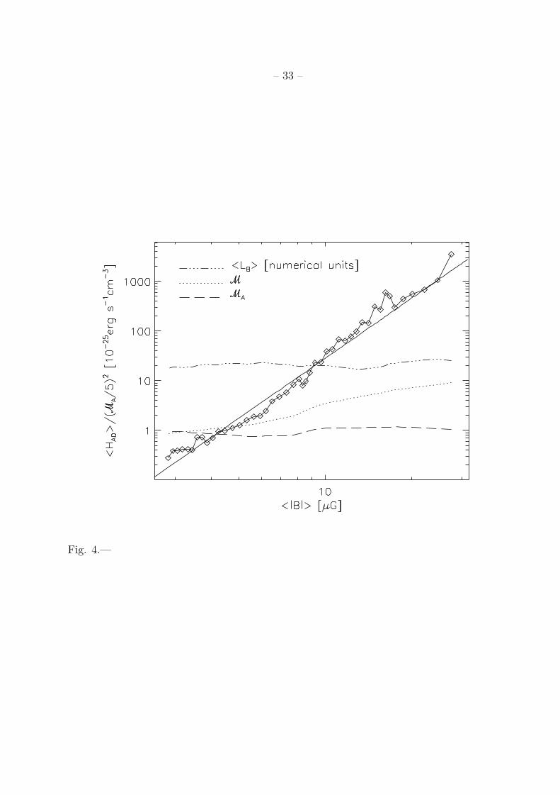
The foregoing results on 〈HAD〉 and the behavior of 〈LB〉 are shown in another form

in Figure 4, which is based on a decaying run with no driving and no mean magnetic field.

The magnetic and kinetic energies are initially in equipartition, and remain so as they

decrease with time. The magnetic field strength shown on the abscissa parameterizes time

from late to early. Figure 4 shows that the sonic Mach number M decays while 〈LB〉 and

MA remain roughly constant. Despite fluctuations, 〈HAD〉 is proportional to 〈| B |〉4 as the

magnetic field decays by an order of magnitude.

We have also studied the dependence of 〈HAD〉 on the ambipolar drift parameter a.

Taken at face value, eqn. (6) predicts 〈HAD〉 ∝ a. But this reasoning does not account

for the dependence of the magnetic field properties on a. As a increases, the increase in

magnetic diffusion decreases the efficiency with which the field is amplified, and increases

LB. The net result is that although 〈HAD〉 is positively correlated with a, the dependence

is weaker than linear over the range of a which we have examined. HAD and LB are plotted

versus a in Figure 5. The plot of 〈HAD〉 versus a is reasonably well fit by 〈HAD〉 ∝ a0.6

over the limited but physically reasonable range 0.15 ≤ a ≤ 1.0. The increase in 〈LB〉 by

roughly a factor of 2 over this range of a accounts for the increase of 〈HAD〉 by roughly a

factor of 4 instead of a factor of 7, as would occur for linear dependence.

– 17 –

Ambipolar drift makes a significant contribution to the rate at which the turbulence

decays. Writing the kinetic energy EK as

EK =1

2〈ρ〉v2

rms = M2A

〈| B |〉28π

(27)

and using eqn. (25) we find the decay time τAD

τAD ≡ EK

〈HAD〉 = 1.3× 106

(〈| B |〉10 µG

)−2( 〈n〉320 cm−3

)3/2

yr. (28)

For comparison, in these models the dynamical time scale L/vrms is about 2.4 × 106 yr.

Thus, as has been argued elsewhere, ambipolar drift is an efficient mechanism for the

dissipation of turbulent energy in molecular clouds (Zweibel & Josafatsson 1983, Elmegreen

1985).

Recently, it has been shown that supersonic hydrodynamic and hydromagnetic

turbulence both decay as EK ∝ t−η, with η ∼ 1 (Mac Low et al 1998, Mac Low 1999). This

decay law implies

dEK

dt∝ −E2

K . (29)

In these models, dissipation occurs primarily in shocks and through the generation and

numerical dissipation of short wavelength Alfven waves; there is no ambipolar drift.

Ambipolar drift actually leads to a similar decay law: 〈HAD〉 ∝ 〈| B |〉2v2rms, which can

be written as E2K since the ratio of magnetic to kinetic energy is fixed in these decaying

models, as shown in Figure 4. Does it matter whether energy is lost by ion-neutral

friction or in shocks? From an observational point of view it does matter, since the peak

temperatures and spatial distribution of the heating in the two cases can be quite different.

We will explore this issue further in a study of thermal equilibrium in molecular clouds

heated by ambipolar drift (Juvela et al. 2000).

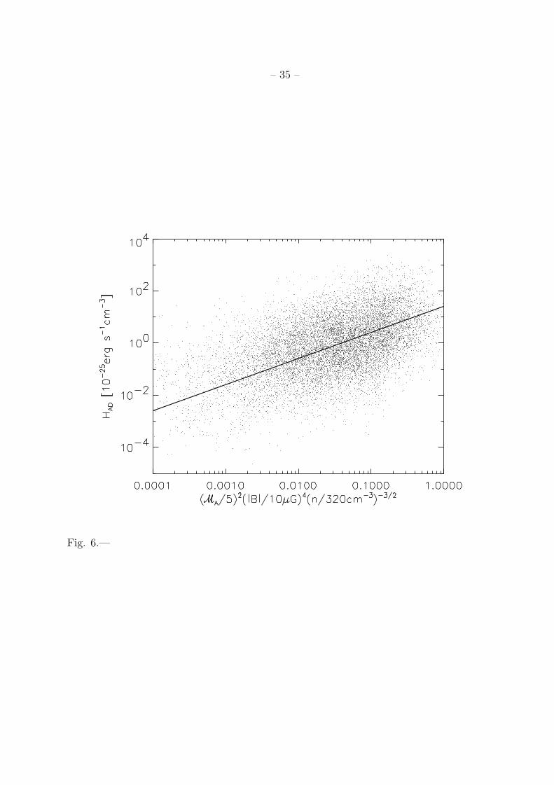
Having established the mean properties, we now describe the pointwise properties of

ambipolar drift heating. Figure 6 is a scatter plot, in dimensional units, of HAD versus

– 18 –

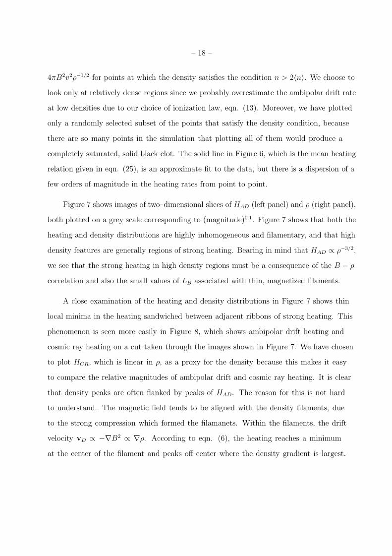
4πB2v2ρ−1/2 for points at which the density satisfies the condition n > 2〈n〉. We choose to

look only at relatively dense regions since we probably overestimate the ambipolar drift rate

at low densities due to our choice of ionization law, eqn. (13). Moreover, we have plotted

only a randomly selected subset of the points that satisfy the density condition, because

there are so many points in the simulation that plotting all of them would produce a

completely saturated, solid black clot. The solid line in Figure 6, which is the mean heating

relation given in eqn. (25), is an approximate fit to the data, but there is a dispersion of a

few orders of magnitude in the heating rates from point to point.

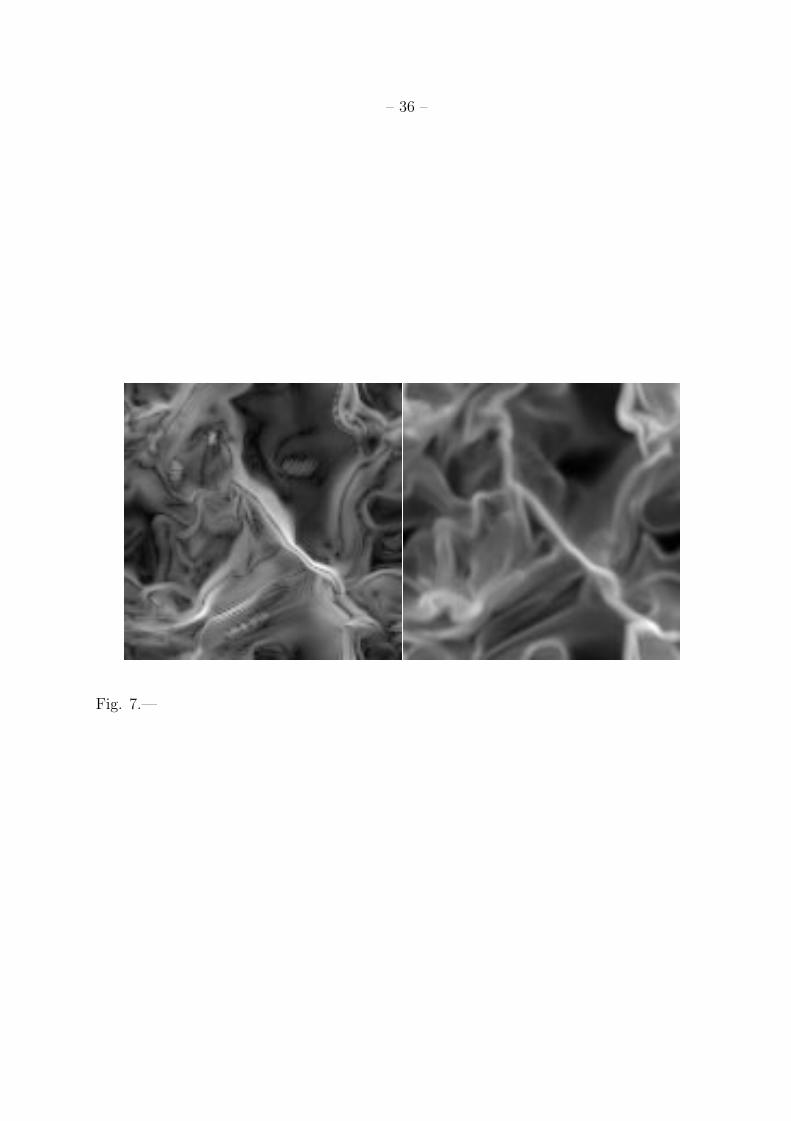
Figure 7 shows images of two–dimensional slices of HAD (left panel) and ρ (right panel),

both plotted on a grey scale corresponding to (magnitude)0.1. Figure 7 shows that both the

heating and density distributions are highly inhomogeneous and filamentary, and that high

density features are generally regions of strong heating. Bearing in mind that HAD ∝ ρ−3/2,

we see that the strong heating in high density regions must be a consequence of the B − ρ

correlation and also the small values of LB associated with thin, magnetized filaments.

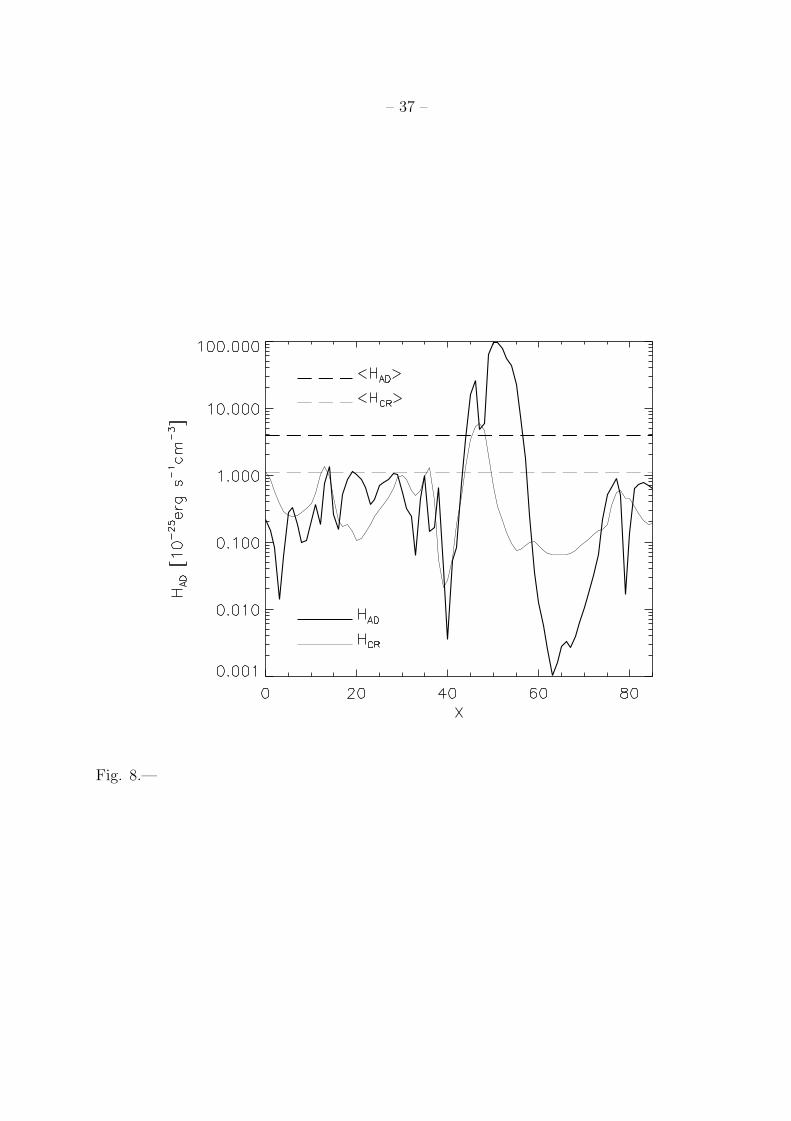
A close examination of the heating and density distributions in Figure 7 shows thin

local minima in the heating sandwiched between adjacent ribbons of strong heating. This

phenomenon is seen more easily in Figure 8, which shows ambipolar drift heating and

cosmic ray heating on a cut taken through the images shown in Figure 7. We have chosen

to plot HCR, which is linear in ρ, as a proxy for the density because this makes it easy

to compare the relative magnitudes of ambipolar drift and cosmic ray heating. It is clear

that density peaks are often flanked by peaks of HAD. The reason for this is not hard

to understand. The magnetic field tends to be aligned with the density filaments, due

to the strong compression which formed the filamanets. Within the filaments, the drift

velocity vD ∝ −∇B2 ∝ ∇ρ. According to eqn. (6), the heating reaches a minimum

at the center of the filament and peaks off center where the density gradient is largest.

– 19 –

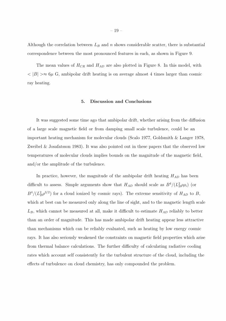
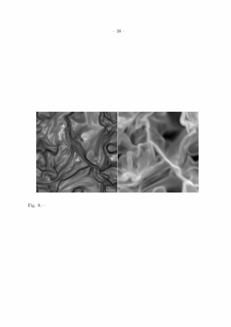
Although the correlation between LB and n shows considerable scatter, there is substantial

correspondence between the most pronounced features in each, as shown in Figure 9.

The mean values of HCR and HAD are also plotted in Figure 8. In this model, with

< |B| >≈ 6µ G, ambipolar drift heating is on average almost 4 times larger than cosmic

ray heating.

5. Discussion and Conclusions

It was suggested some time ago that ambipolar drift, whether arising from the diffusion

of a large scale magnetic field or from damping small scale turbulence, could be an

important heating mechanism for molecular clouds (Scalo 1977, Goldsmith & Langer 1978,

Zweibel & Josafatsson 1983). It was also pointed out in these papers that the observed low

temperatures of molecular clouds implies bounds on the magnitude of the magnetic field,

and/or the amplitude of the turbulence.

In practice, however, the magnitude of the ambipolar drift heating HAD has been

difficult to assess. Simple arguments show that HAD should scale as B4/(L2Bρρi) (or

B4/(L2Bρ3/2) for a cloud ionized by cosmic rays). The extreme sensitivity of HAD to B,

which at best can be measured only along the line of sight, and to the magnetic length scale

LB, which cannot be measured at all, make it difficult to estimate HAD reliably to better

than an order of magnitude. This has made ambipolar drift heating appear less attractive

than mechanisms which can be reliably evaluated, such as heating by low energy cosmic

rays. It has also seriously weakened the constraints on magnetic field properties which arise

from thermal balance calculations. The further difficulty of calculating radiative cooling

rates which account self consistently for the turbulent structure of the cloud, including the

effects of turbulence on cloud chemistry, has only compounded the problem.

– 20 –

For several reasons, the role of ambipolar drift heating in the thermal equilibrium

of clouds is becoming more open to assessment, and hence more interesting. Reliable

maps of temperature, density, magnetic field, and velocity structure are now available for

more clouds than ever before, permitting correlation studies of cloud temperature with

other properties. Detailed numerical models of turbulent molecular clouds, and improved

calculations of cooling rates and cloud chemistry, are now feasible. Thermal balance

calculations which include ambipolar drift heating, compared with observations, can now

lead to meaningful diagnostics of magnetic fields and dynamical properties of molecular

clouds.

In this paper we have used simulations of turbulent, magnetized molecular clouds to

study the properties of heating by ambipolar drift. The models are self consistent in the

sense that we include ambipolar drift in calculating the dynamics of the cloud and the

evolution of the magnetic field. We have found that a realistic amount of ambipolar drift

in a simulation with the highest numerical resolution practical for us (N = 1283 mesh

points) imparts a physical as opposed to numerical diffusivity to the cloud which makes

it just possible to capture all of the relevant length scales. The models can be scaled

to approximate the sizes, densities, velocity dispersions, and magnetic field strengths of

observed clouds. As our simulations do not include self gravity, we focus on ambipolar drift

heating due to turbulence rather than due to the systematic redistribution of a large scale

field in quiescent, gravitationally contracting structures.

The main result of our paper is an empirical formula for the volume averaged heating

rate, 〈HAD〉, given in eqn. (25) : 〈HAD〉 ∝ 〈| B |〉4M2A/ρρi, or 〈HAD〉 ∝ 〈| B |〉2v2

rms/ρi. As

shown in Figure 2, the fit is very good, and comes about because the magnetic length scale

LB is inversely proportional to MA (Figure 3). Our scaling law for 〈HAD〉 makes it possible

to estimate the ambipolar drift heating rate in individual clouds much more accurately than

– 21 –

before: the uncertainty in the value of B is only squared, not raised to the fourth power,

and LB is replaced by the more readily measurable rms velocity, or line width.

Furthermore, 〈HAD〉 turns out to be interestingly large, exceeding, for moderately

large field strength, the mean cosmic ray heating rates HCR. And, the turbulent dissipation

times associated with ambipolar drift heating are of order the dynamical crossing times in

our models, suggesting, as argued elsewhere, that the turbulence in molecular clouds must

be driven continuously.

In some respects, however, the conventional wisdom that HAD is difficult to estimate

is borne out by its large range in value from point to point within any particular model.

Despite the excellent correlation of the global heating rate with averaged quantities, a

scatter plot of HAD versus the pointwise values of the same quantities which go into the

mean relation eqn. (25) shows dispersion of a few orders of magnitude about the mean, as

shown in Figure 6, (although the relation based on global averages is an approximate fit to

the centroid of the distribution). In models with a fairly weak magnetic field and a tight

B − ρ relation, the correspondence between density and HAD is quite good, even down to

individual features (Figure 7).

We are presently studying the thermal equilibrium problem with a Monte Carlo

treatment of radiative transfer. For the present, however, we note that standard calculations

of radiative cooling rates in the temperature and density regimes of interest to us here

(T ∼ 10K − 40K, n ∼ 103 − 104) scale with temperature as T 2.2−2.7 (Goldsmith & Langer

1978, Neufeld, Lepp, & Melnick 1995). Therefore, if ambipolar drift is the dominant

heating mechanism, there should be a relation with temperature and line width of the form

T ∝ ∆v.74−.91. The exponent of this relation could be reduced, due to the dependence of

the cooling rate on the velocity gradient in the gas. In fact, a positive correlation, but with

a somewhat shallower slope, has recently been reported (Jijina, Myers, & Adams 1999). In

– 22 –

general, however, we would expect that any model in which the dissipation of turbulence

contributes to heating would produce a positive T −∆v correlation.

We thank Ted Bergin, Alyssa Goodman, Mika Juvela and Phil Myers for reading the

manuscript and providing useful comments. We are happy to acknowledge support by

NSF Grant AST 9800616 and NASA Grant NAG5-4063 to the University of Colorado,

and support by the Danish National Research Foundation through its establishment of the

Theoretical Astrophysics Center.

– 23 –

REFERENCES

Brandenburg, A., Nordlund, A., Stein, R.F., & Torkelsson, U. 1995, ApJ, 446, 741

Brandenburg, A. & Zweibel, E.G. 1994, ApJ, 427, L91

Brandenburg, A. & Zweibel, E.G. 1995, ApJ, 448, 734

Caselli, P., Walmsley, C.M., Terzieva, R., Herbst, E. 1998, ApJ, 499, 234

de Jong, T., Dalgarno, A., & Boland, W. 1980, A&A, 91, 68

Draine, B.T. 1980, ApJ, 241, 1021

Draine, B.T. 1986, MNRAS, 220, 133

Draine, B.T. & McKee, C.F. 1993, ARA&A

Draine, B.T., Roberge, W. G., & Dalgarno, A. 1983, ApJ, 264, 485

Elmegreen, B.G. 1985, ApJ, 299, 196

Galsgaard, K., Nordlund, A. 1996, Journal of Geophysical Research, 101(A6), 13445

Galsgaard, K., Nordlund, A. 1997, Journal of Geophysical Research, 102, 231

Goldreich, P. & Kwan, J. 1974, ApJ, 189, 441

Goldsmith, P.F. & Langer, W.D. 1978, ApJ, 222, 881

Hawley, J.F. & Stone, J.M. 1998, ApJ, 501, 758

Hyman, J. 1979, in R. Vichnevetsky, R. S. Stepleman (eds.), Adv. in Comp. Meth. for

PDE’s—III, 313

Jijina, J., Myers, P. C., & Adams, F. C. 1999, ApJS, in press

Juvela, M., Padoan, P., Nordlund, A., & Zweibel, E.G. 2000 to be submitted to ApJ

Kolmogorov, A. N. 1941, Dokl. Akad. Nauk. SSSR, 30, 301

– 24 –

Larson, R.B. 1981, MNRAS, 194, 809

Mac Low, M.-M., Norman, M.L., Konigl, A., & Wardle, M. 1995, ApJ, 442, 726

Mac Low, M.-M., & Smith, M.D. 1997, ApJ, 491, 596

Mac Low, M.-M., Klessen, R.S., Burkert, A., Smith, M.D, & Kessel, O. 1998, in J. Franco,

A. Carraminana (eds.), Interstellar Turbulence, Cambridge University Press

Mac Low, M.-M. 1999, ApJ, in press

McKee, C.F. 1989, ApJ, 345, 782

McKee, C.F., Zweibel, E.G., Heiles, C. & Goodman, A.A. 1993, in Protostars & Planets

III, ed. E.H. Levy & J.I. Lunine, U. of Arizona Press, Tucson, 327

Mullan, D.J. 1971, MNRAS, 153, 145

Nakano, T. & Umebayashi, T. 1986, MNRAS, 218, 663

Neufeld, D.A., Lepp, S., & Melnick, G.J. 1995, ApJ, 100, 132

Nordlund, A. & Galsgaard, K. 1997, A 3D MHD Code for Parallel Computers, Technical

report, Astronomical Observatory, Copenhagen University

Nordlund, A., Stein, R.F., & Galsgaard, K. 1996, in J. Wazniewski (ed.), Proceedings from

the PARA95 workshop, Vol. 1041 of Lecture Notes in Computer Science, Springer,

p. 450

Padoan, P., Juvela, M., Bally, J., & Nordlund, A. 1998, ApJ, 504, 300

Padoan, P. & Nordlund, A. 1999, ApJ, in press

Scalo, J.M. 1977, ApJ, 213, 705

Scalo, J.M. & Pumphrey, W.A. 1982, ApJ, 258, L29

Shu, F.H. 1983, ApJ, 273, 202

Solomon, P.M., Rivolo, A.R., Barrett, J., & Yahil, A. 1987, ApJ, 319, 730

– 25 –

Stone, J.M., Ostriker, E.C., & Gammie, C.F. 1998, ApJ, 508, L99

Toth, G. 1994, ApJ, 425, 171

Williams, J.P., Bergin, A.B., Caselli, P., Myers, P.C., & Plume, R. 1998, ApJ, 503, 689

Zweibel, E.G. & Brandenburg, A. 1997, ApJ, 478, 563

Zweibel, E.G. & Josafatsson, K. 1983, ApJ, 270, 511

This manuscript was prepared with the AAS LATEX macros v3.0.

– 26 –

FIGURE AND TABLE CAPTIONS

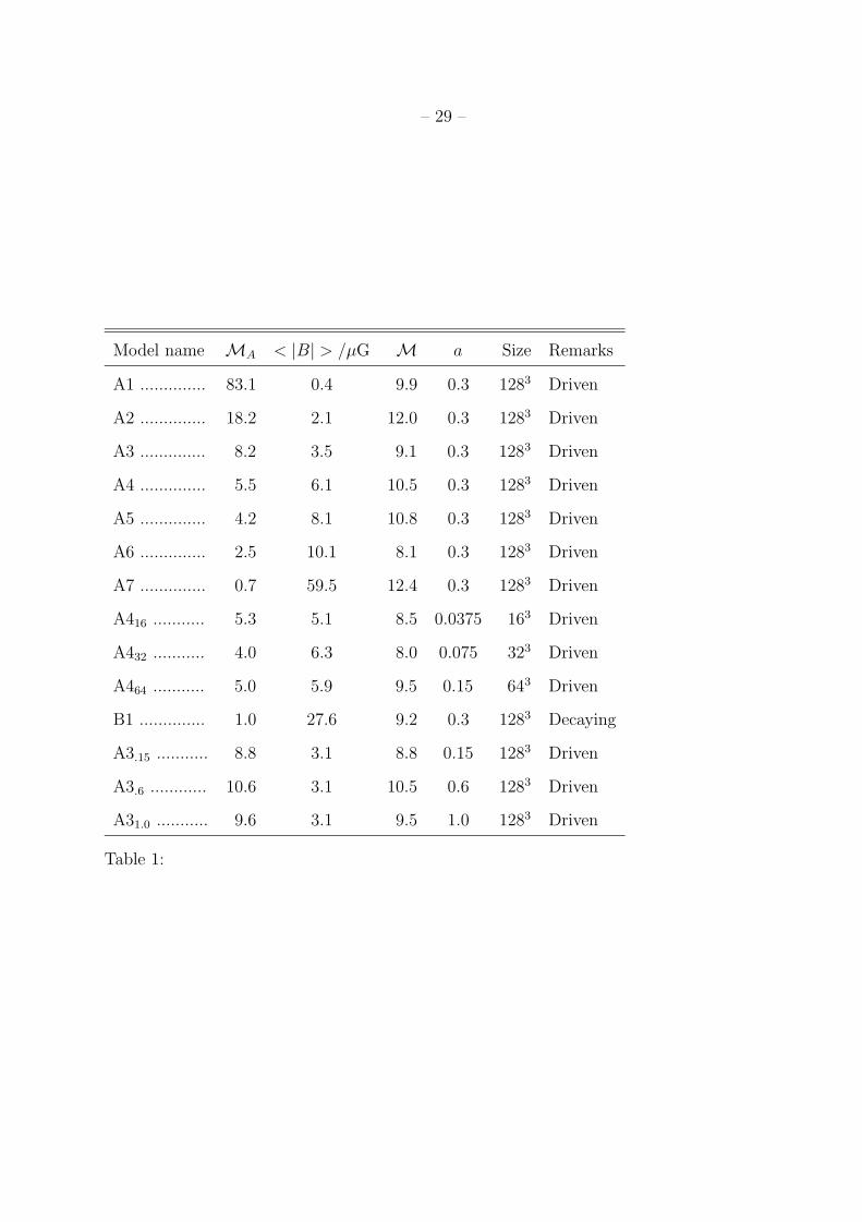
Table 1: Volume and time averaged parameters of the numerical experiments. In the

case of the decaying experiment B1, the initial values of 〈|B|〉 and M are given, instead of

their time averaged values.

Figure 1: Left panel: Volume averaged ambipolar heating rate per unit volume as a

function of the average magnetic field strength, in snapshots from simulations with different

size of the numerical mesh. The heating rate has been divided by its expected value (see

§4) in a model with MA = 5 and 〈|B|〉 = 10 µG. Right panel: Heating rate averaged over

the different snapshots used in the left panel, versus the linear size of the computational

mesh. The heating rate shows a clear trend to convergence.

Figure 2: Volume averaged ambipolar drift heating rate, divided by the square of

the rms Alfvenic Mach number, versus the averaged magnetic field strength, in randomly

driven 1283 simulations, with roughly constant ordinary rms Mach number, M ≈ 10, and

〈n〉 = 320 cm−3. The continuous line shows a 〈|B|〉4 dependence, while the dashed line is

the cosmic ray heating rate per unit volume, also divided by M2A.

Figure 3: Magnetic length scale (see text) versus the rms Alfvenic Mach number of the

flow, in 1283 simulations. The upper dashed line marks the physical size of the simulation

box, and the lower dashed line the physical size that corresponds to the numerical resolution

(taken as two grid cells). The continuous line shows a M−1A dependence. LB is roughly

proportional to M−1A , in a range of values of MA typical of conditions in molecular clouds,

while it departs from that dependence around MA ≈ 10, where LB approaches the limit of

the numerical resolution.

– 27 –

Figure 4: Volume averaged ambipolar drift heating rate per unit volume, divided by

the square of the rms Alfvenic Mach number, versus the averaged magnetic field strength,

in a decaying 1283 simulation. The continuous line shows a 〈|B|〉4 dependence. Kinetic and

magnetic energy decay at approximately the same rate, and so the flow is in approximate

equipartition at all times, MA ≈ 1. Also the magnetic length scale LB is approximately

constant, which proves that it depends only on MA.

Figure 5: Upper panels: Volume averaged ambipolar drift heating rate per unit

volume, divided by its expected value for a = 0.3, according to eqn. (25). Different symbols

represent different values of the ambipolar diffusion parameter, a. Lower panels: Magnetic

lengthscale for different values of the ambipolar diffusion parameter.

Figure 6: Local value of the ambipolar drift heating rate per unit volume, versus

its expected average value for the average parameters used in the simulation: MA = 5,

〈|B|〉 = 10 µG, and 〈n〉 = 320 cm−3. The local heating rate spans a range of values of

about 8 orders of magnitude, but it also follows the value expected for the volume averaged

heating rate, shown by the continuous line. Only points with n > 2〈n〉 have been used in

the scatter plot (see text).

Figure 7: Images of two–dimensional slices of ambipolar diffusion heating rate per

unit volume (left) and of gas density (right), from a snapshot of a 1283 simulation, with

MA ≈ 5, and 〈|B|〉 ≈ 6µ G. The intensity in the image is proportional to H0.1AD (left) and

n0.1 (right).

Figure 8: Local ambipolar drift heating rate (thick line) and cosmic ray heating rate

– 28 –

(thin line) per unit volume. It is a cut through the slice presented in Fig. 7. The dashed

lines show the values of the heating rates averaged over the whole computational box.

Figure 9: Images of two–dimensional slices of magnetic length scale (left) and gas

density (right). The slice is the same used in Fig. 7, and the intensity in the image is

proportional to L0.1B (left) and n0.1 (right).

– 29 –

Model name MA < |B| > /µG M a Size Remarks

A1 .............. 83.1 0.4 9.9 0.3 1283 Driven

A2 .............. 18.2 2.1 12.0 0.3 1283 Driven

A3 .............. 8.2 3.5 9.1 0.3 1283 Driven

A4 .............. 5.5 6.1 10.5 0.3 1283 Driven

A5 .............. 4.2 8.1 10.8 0.3 1283 Driven

A6 .............. 2.5 10.1 8.1 0.3 1283 Driven

A7 .............. 0.7 59.5 12.4 0.3 1283 Driven

A416 ........... 5.3 5.1 8.5 0.0375 163 Driven

A432 ........... 4.0 6.3 8.0 0.075 323 Driven

A464 ........... 5.0 5.9 9.5 0.15 643 Driven

B1 .............. 1.0 27.6 9.2 0.3 1283 Decaying

A3.15 ........... 8.8 3.1 8.8 0.15 1283 Driven

A3.6 ............ 10.6 3.1 10.5 0.6 1283 Driven

A31.0 ........... 9.6 3.1 9.5 1.0 1283 Driven

Table 1:

– 30 –

Fig. 1.—

– 31 –

Fig. 2.—

– 32 –

Fig. 3.—

– 33 –

Fig. 4.—

– 34 –

Fig. 5.—

– 35 –

Fig. 6.—

– 36 –

Fig. 7.—

– 37 –

Fig. 8.—

– 38 –

Fig. 9.—