Ambiguous Policy Announcements

Claudio MichelacciEIEF and CEPR

Luigi Paciello∗

EIEF and CEPR

October 31, 2016

Preliminary and Incomplete

Abstract

We study the effects of monetary policy announcements in a New Keynesianmodel, where ambiguity averse households with heterogenous net financial wealth usea worst-case criterion to evaluate the credibility of announcements. An announce-ment of a future loosening in monetary policy leads to rebalancing in financial assetpositions, can cause credit crunches, and might be contractionary in the interim pe-riod before implementation. This is because households with positive net financialwealth (creditors) are the most likely to believe the announcement, due to the wealthlosses that future monetary policy can cause to them. And when creditors believethe announcement more than debtors do, the wealth losses that creditors expect toincur are larger than the wealth gains that debtors expect to realize. So aggregatenet wealth is perceived to fall, and the economy can contract due to lack of aggregatedemand, which is more likely when wealth inequality is large. We evaluate the impor-tance of this mechanism by focusing on the start of the Forward Guidance practiceby the ECB in July 2013. We show that the inflation expectations of households haveresponded in accordance with the theory. After matching the entire distribution ofEuropean households’ net financial wealth, we find that the ECB announcement iscontractionary in our model. Generally, redistributing expected future wealth mighthave unintended perverse effects when agents are ambiguity averse.

∗We would like to thank Manuel Amador, Gene Ambrocio, Philippe Andrade, Francesco Caselli, MichaelElsby, Nicola Gennaioli, Luigi Guiso, Javier Suarez, Giovanni Violante, and Mirko Wiederholt for usefulcomments, as well as seminar participants at CUHK, HKUST, SciencesPo, and SED meetings. We ac-knowledge the financial support of the European Research Council (ERC Advanced Grant 293692, ERCStarting Grant 676846). E-mail: c.michelacci1968@gmail.com, gigipaciello@gmail.com. Postal address:EIEF, Via Sallustiana, 62, 00187 Roma, Italy.

1 Introduction

Policy makers often rely on announcements about future reforms of economic institutions

or future changes in fiscal or monetary policy to stimulate the economy in the short run.

Once implemented, these policies typically have important redistributive implications. For

example during the recent Great Recession and since short term nominal interest rates had

hit the zero lower bound, Central Banks have relied extensively on announcements about

future changes in monetary policy to raise today inflation and stimulate the economy, a

practice which is generally known as Forward Guidance. And it is well known that higher

inflation tends to redistribute wealth from creditors to debtors (Fisher 1933, Doepke and

Schneider 2006, and Adam and Zhu 2015). In this paper we show that, when agents are am-

biguity averse, policy announcements might have unintended perverse effects in the interim

period before the policy is actually implemented. Generally the effect of the announcement

depends on (i) the amount of redistribution induced by the policy if implemented, (ii) the

concentration of future hypothetical wealth losses, and (iii) the (endogenous) correlation

between agents’ wealth and their changes in expectations at the time of the announcement.

To show these points, we consider the effects of monetary policy announcements in a

New Keynesian model, where ambiguity averse households with heterogenous net financial

wealth use a worst-case criterion to evaluate the credibility of announcements, according to

the Maximin preferences specification proposed by Gilboa and Schmeidler (1989). Ambigu-

ity aversion is a natural paradigm when characterizing the behavior of households who do

not know the probability distribution of outcomes, which is likely to happen when house-

holds have to deal with news about unfamiliar contingencies, as for example in the case of

announcements about future unconventional policies in an unusual economic environment.

We focus on the effects of announcements of future changes in real rates due to changes

in inflation and/or nominal rates, in an economy which is initially in a steady state equi-

librium. If implemented, a reduction in real rates tends to stimulate the consumption of

agents with negative net financial wealth (debtors) through both a substitution and an

income effect. However, for agents with positive net financial wealth (creditors), a change

in real rates involves a substitution and an income effect on consumption which tends to

have opposite effects on consumption. This is because a fall in real returns reduces the cap-

ital income that pertains to creditors. As a result, creditors are more likely to believe the

announcement of a future loosening in monetary policy than debtors are, because the worst-

case scenario for creditors—at least for those with sufficiently large net financial wealth—

is that real rates and thereby their financial income will actually fall. However, if creditors

believe the announcement more than debtors do, the wealth losses that creditors expect

1

to incur are larger than the gains that debtors expect to realize and as a result aggregate

net wealth—equal to the sum of the expected wealth of creditors and debtors—is perceived

to fall. This is what we call the forward misguidance effect, which can be strong enough

to dominate the conventional substitution effect and thereby to lead to a contraction in

aggregate activity due to lack of aggregate demand. This fall in demand is more likely when

wealth inequality is large so that the capital losses induced by future monetary policy are

concentrated among a small group of relatively wealthy households. Generally, as a result

of the announcement of a future loosening in monetary policy, the real rate expected by

creditors is smaller than the real rate expected by debtors, which leads to a rebalancing in

the financial asset positions of agents and can even cause credit crunches, which happen

because agents stop trading in financial markets so as to get fully insured against future

changes in monetary policy.

An announcement of a future tightening in monetary policy with an associated future

increase in real rates is unambiguously contractionary in our model. In this case debtors

are the most likely to believe the announcement and for them the future increase in real

rates leads to a reduction in their consumption through a substitution and an income effect

which both work in the direction of reducing consumption. So aggregate consumption and

thereby output unambiguously fall. The fall in output is larger than the one that would

arise in an hypothetical equilibrium where the announcement is fully believed by all agents

in the economy. This again emphasizes that, under ambiguity aversion, redistributing

future expected wealth is a negative-sum game.

We evaluate the importance of this mechanism by focusing on the start of the Forward

Guidance practice by the ECB on 4 July 2013.1 After the announcement, long-term gov-

ernment bonds yields and EONIA swap rates have fallen by around 10-15 basis points at

maturities between 2 and 4 years, see Coeure (2013), ECB (2014), and Section 5. There

is evidence that the inflation expectations of households have responded to the announce-

ment as predicted by the misguidance effect. Figure 1 shows the evolution of households’

expected inflation, in panel (a), and realized inflation in panel (b) in the Euro 11 coun-

tries, separately for the group of creditor countries (as a blue dashed line) and of debtor

countries (as a green dotted line). Creditor countries are defined as those that at the

time of the ECB announcement had a positive Net Foreign Asset position, which include

Austria, Finland, Germany, Luxembourg, and Netherlands. Debtor countries are all the

others. The difference between the two lines corresponds to the red solid line in the figure.

1On that date the ECB Governing Council has started its Forward Guidance practice by announcingthat “it expected the key ECB interest rates to remain at present or lower levels for an extended period oftime.”

2

Figure 1: Forward Guidance in Euro 11: Expected and realized inflation

46

810

12D

iffer

ence

3020

105

Infla

tion

expe

ctat

ions

12q4 13q1 13q2 13q3 13q4 14q1 14q2 14q3Year:quarter

Creditors Debtors Difference

(a) Expected change in trend inflation

32

10

Diff

eren

ce

32

10

Cor

e In

flatio

n

12q4 13q1 13q2 13q3 13q4 14q1 14q2 14q3Year:quarter

Creditors Debtors Difference

(b) Actual Inflation

Notes: Core Inflation is yearly log differences in consumer prices excluding energy and seasonal foodmultiplied by 100. Expectations are calculated in terms of balances—differences between peopleproviding positive and negative answer. Price expectations come from the following question: “Bycomparison with the past 12 months, how do you expect that consumer prices will develop in thenext 12 months? They will (i) increase more rapidly; (ii) increase at the same rate; (iii) increase ata slower rate; (iv) stay about the same; (v) fall. Probabilities are calculated in terms of balances:differences between people saying that he answer is very likely versus people saying the answer it isunlikely. Price expectations are calculated as equal to (fi + 1/2fii − 1/2fiv − fv)× 10, where fj is thefraction of individuals who opted for option j = i, ii, iii, iv, v in the survey. Creditor countries areAustria, Finland, Germany, Luxembourg, and Netherlands. Others countries include all the remainingcountries in the group of Euro 11 countries. Source of data: ECB, Joint Harmonized Programme ofBusiness and Consumer Surveys by European Commission and External Wealth of Nation Mark II(EWN).

The area in grey identifies the quarter of the announcement. Inflation has kept falling

after the announcement, which is consistent with the relatively muted effects of Forward

Guidance estimated in the US (Del Negro, Giannoni, and Patterson 2015). Interestingly,

after the announcement, inflation has kept falling at a higher speed in creditor countries

than in debtor countries, see panel (b). Still, and relative to trend, inflation expectations

have been revised upwards only in creditor countries, whereas they have remained stable

in debtor countries, see panel (a). As a result the difference in inflation expectations be-

tween creditor and debtor countries has increased, which, together with the evidence for

actual inflation above, implies that the wedge between expected future inflation and future

realized inflation has widened in creditor countries relative to debtor countries.

To provide further evidence in favor of the misguidance effect, we rely on a Difference-

in-Differences identification strategy using Italian provinces, which differ substantially in

3

their net financial wealth and are subject to the same country specific shocks. We exploit a

unique quarterly-frequency dataset with information on both expected and realized inflation

at a very disaggregated level. In each province we construct a measure of the inflation

expectation bias of households by calculating the difference between today expected future

inflation and future realized inflation. We classify provinces according to the fraction of

households in the province who have positive net financial wealth (creditor households). We

show that, in response to the ECB announcement, provinces with a larger share of creditor

households experience a relative increase in their inflation expectation bias: roughly, a one

standard deviation increase in the share of creditor households in the province is associated

with an after-the-announcement relative increase in the expectation bias of 9 basis points.

To study the quantitative relevance of the effect, we calibrate our heterogenous agents

new Keynesian model to match data from the Household Finance and Consumption Sur-

vey (HFCS) on the entire distribution of European households’ net financial wealth. We

calibrate the ECB announcement to match the response on 4 July 2013 of the yield curve

of interest rates at all maturities between 2 and 10 years. We find that in our model

the output effect of the ECB announcement is substantially muted relative to the effect

that would arise in the alternative standard benchmark where all households fully believe

the announcement. Under our preferred parametrization, the announcement is actually

contractionary, with a cumulated output loss of 1.6% in the fifteen months before imple-

mentation, which should be compared with the cumulated output gain of almost 6% under

the alternative benchmark.

Relation to the Literature. Forward Guidance has become a central tool of monetary policy

during the current recession because conventional expansionary monetary policies were no

longer available as short term interest rates hit the zero lower bound. And there is a

growing literature studying optimal monetary policy in a liquidity trap (Eggertsson and

Woodford 2003) as well as the effects of Forward Guidance (Del Negro, Giannoni, and

Patterson 2015, Swanson 2016). From the point of view of conventional New Keynesian

sticky price models it is a puzzle why Forward Guidance announcements have been little

effective in stimulating the economy and moving it out of a liquidity a trap, and some

papers have proposed explanations for this puzzle, see Andrade, Gaballo, Mengus, and

Mojon (2015), Caballero and Farhi (2014), Kaplan, Moll, and Violante (2016b), McKay,

Nakamura, and Steinsson (2015) and Wiederholt (2014). In this paper we abstract away

from the reason why the monetary authority relies on announcements to stimulate the

economy. We just emphasize, that, under ambiguity aversion, announcements of a future

loosening in monetary policy are more likely to affect the expectations of agents with large

net financial wealth than those of agents with negative financial wealth, and because of

4

this the economy can even contract in the presence of large financial imbalances.

It has been known at least since Fisher (1933) that expansionary monetary policy redis-

tributes wealth from creditors to debtors. It has also been observed that this redistribution

could be expansionary on aggregate demand because agents differ either in their marginal

propensity to consume out of wealth, as first emphasized by Tobin (1982), or in the liq-

uidity and term structure of their portfolios, as in Kaplan, Moll, and Violante (2016a) and

Auclert (2015) respectively. However, see Doepke, Schneider, and Selezneva (2015) for an

overlapping generation model where this redistribution makes aggregate consumption fall.

Here we focus on redistributing future expected wealth, which under ambiguity aversion is

typically a negative-sum game, because net losers out of the redistribution tend to believe

any news about the future more than net winners do.

Other papers have emphasized that ambiguity aversion matters for business cycle anal-

ysis. Ilut and Schneider (2014) show that shocks to the amount of ambiguity can be an

important source of business cycle volatility. Ilut, Valchev, and Vincent (2016) study the

implication of ambiguity aversion for sticky prices. Backus, Ferriere, and Zin (2015) fo-

cus on asset pricing, while Ilut, Krivenko, and Schneider (2015) provide methods to study

dynamic economies where ambiguity averse agents differ in their perception of exogenous

shocks and study the implications for precautionary savings, asset premia and insurance

gains. Here we focus on the effects of announcements and more generally of news about

the future and how they interact with wealth inequality and redistribution.

Recent research has emphasized that there is substantial heterogeneity in the inflation

expectations of agents, see for example Coibion, Gorodnichenko, and Kumar (2015) for

evidence. Here we emphasize that, when agents are ambiguity averse, changes in inflation

expectations of agents are related to their wealth position.

Section 2 provides some evidence. Section 3 characterizes the economy. Section 4 studies

the effect of monetary policy announcements in a simple case. Section 5 evaluates quanti-

tatively the effect of the ECB announcement on July 2103. Section 6 studies robustness.

Section 7 concludes. The Appendix contains details on data and model computation.

2 Some more evidence on the misguidance effect

Figure 1 indicates that, in response to the Forward Guidance announcement by the ECB,

the inflation expectations of households have responded more in creditor than in debtor

countries, which is evidence consistent with a misguidance effect. However, aggregate

country-level data do not provide information on the within-country distribution of house-

holds’ net financial assets. Moreover, country-specific asymmetric shocks have played an

5

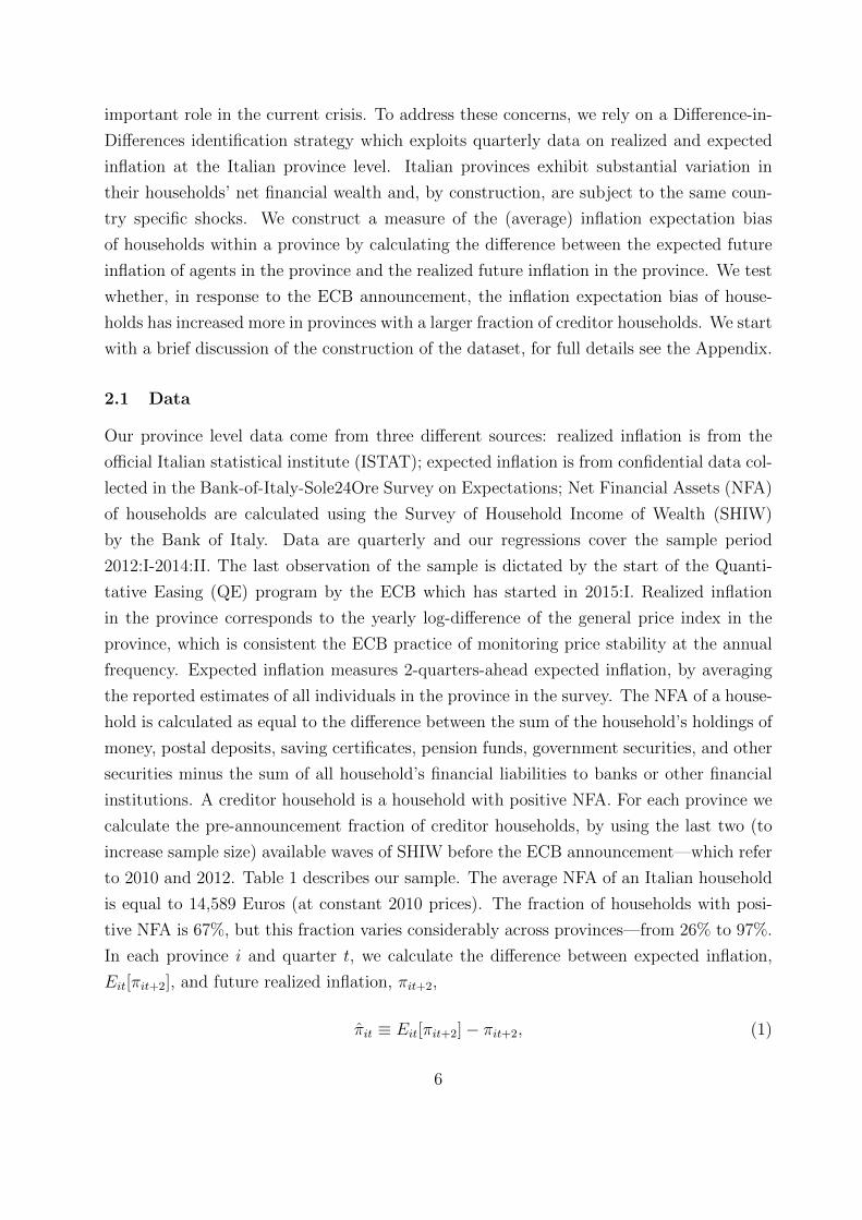
important role in the current crisis. To address these concerns, we rely on a Difference-in-

Differences identification strategy which exploits quarterly data on realized and expected

inflation at the Italian province level. Italian provinces exhibit substantial variation in

their households’ net financial wealth and, by construction, are subject to the same coun-

try specific shocks. We construct a measure of the (average) inflation expectation bias

of households within a province by calculating the difference between the expected future

inflation of agents in the province and the realized future inflation in the province. We test

whether, in response to the ECB announcement, the inflation expectation bias of house-

holds has increased more in provinces with a larger fraction of creditor households. We start

with a brief discussion of the construction of the dataset, for full details see the Appendix.

2.1 Data

Our province level data come from three different sources: realized inflation is from the

official Italian statistical institute (ISTAT); expected inflation is from confidential data col-

lected in the Bank-of-Italy-Sole24Ore Survey on Expectations; Net Financial Assets (NFA)

of households are calculated using the Survey of Household Income of Wealth (SHIW)

by the Bank of Italy. Data are quarterly and our regressions cover the sample period

2012:I-2014:II. The last observation of the sample is dictated by the start of the Quanti-

tative Easing (QE) program by the ECB which has started in 2015:I. Realized inflation

in the province corresponds to the yearly log-difference of the general price index in the

province, which is consistent the ECB practice of monitoring price stability at the annual

frequency. Expected inflation measures 2-quarters-ahead expected inflation, by averaging

the reported estimates of all individuals in the province in the survey. The NFA of a house-

hold is calculated as equal to the difference between the sum of the household’s holdings of

money, postal deposits, saving certificates, pension funds, government securities, and other

securities minus the sum of all household’s financial liabilities to banks or other financial

institutions. A creditor household is a household with positive NFA. For each province we

calculate the pre-announcement fraction of creditor households, by using the last two (to

increase sample size) available waves of SHIW before the ECB announcement—which refer

to 2010 and 2012. Table 1 describes our sample. The average NFA of an Italian household

is equal to 14,589 Euros (at constant 2010 prices). The fraction of households with posi-

tive NFA is 67%, but this fraction varies considerably across provinces—from 26% to 97%.

In each province i and quarter t, we calculate the difference between expected inflation,

Eit[πit+2], and future realized inflation, πit+2,

πit ≡ Eit[πit+2]− πit+2, (1)

6

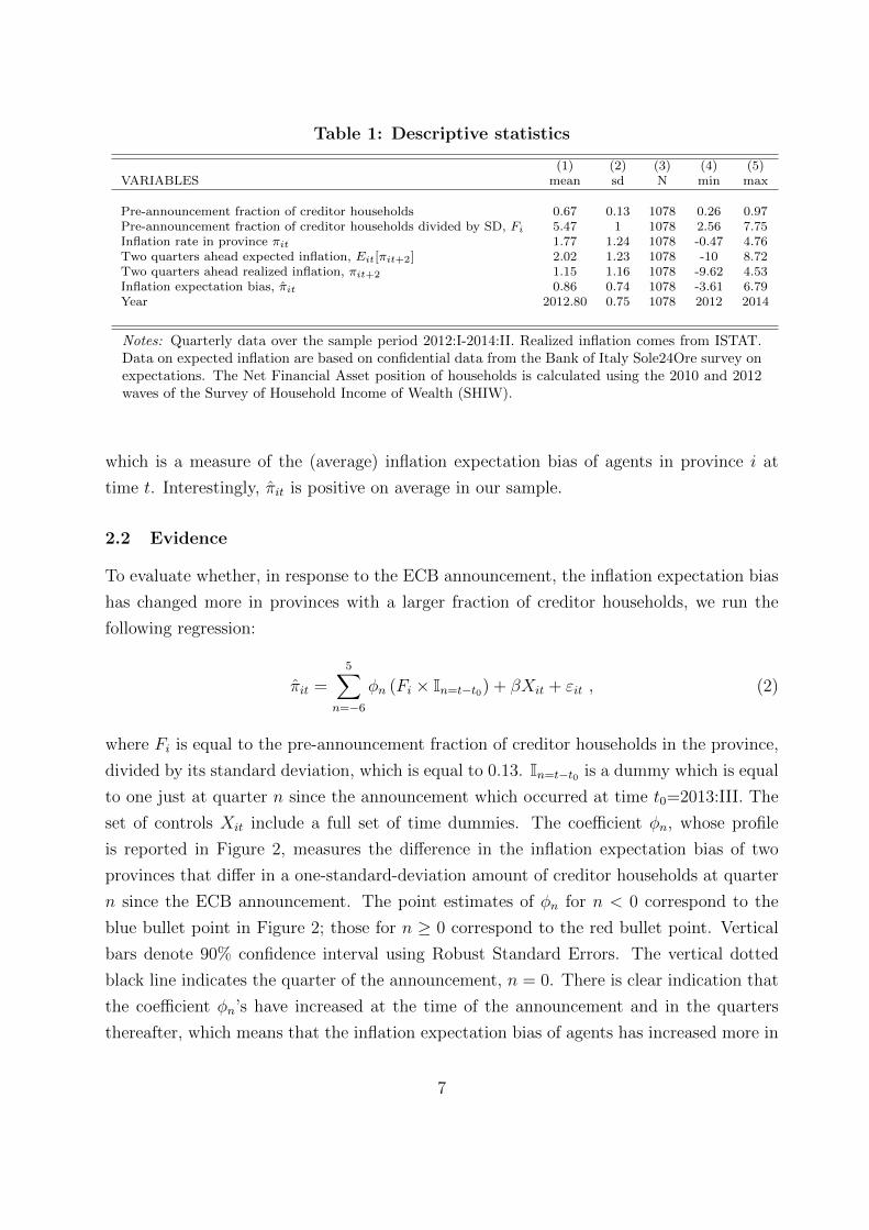
Table 1: Descriptive statistics

(1) (2) (3) (4) (5)VARIABLES mean sd N min max

Pre-announcement fraction of creditor households 0.67 0.13 1078 0.26 0.97Pre-announcement fraction of creditor households divided by SD, Fi 5.47 1 1078 2.56 7.75Inflation rate in province πit 1.77 1.24 1078 -0.47 4.76Two quarters ahead expected inflation, Eit[πit+2] 2.02 1.23 1078 -10 8.72Two quarters ahead realized inflation, πit+2 1.15 1.16 1078 -9.62 4.53Inflation expectation bias, πit 0.86 0.74 1078 -3.61 6.79Year 2012.80 0.75 1078 2012 2014

Notes: Quarterly data over the sample period 2012:I-2014:II. Realized inflation comes from ISTAT.Data on expected inflation are based on confidential data from the Bank of Italy Sole24Ore survey onexpectations. The Net Financial Asset position of households is calculated using the 2010 and 2012waves of the Survey of Household Income of Wealth (SHIW).

which is a measure of the (average) inflation expectation bias of agents in province i at

time t. Interestingly, πit is positive on average in our sample.

2.2 Evidence

To evaluate whether, in response to the ECB announcement, the inflation expectation bias

has changed more in provinces with a larger fraction of creditor households, we run the

following regression:

πit =5∑

n=−6

φn (Fi × In=t−t0) + βXit + εit , (2)

where Fi is equal to the pre-announcement fraction of creditor households in the province,

divided by its standard deviation, which is equal to 0.13. In=t−t0 is a dummy which is equal

to one just at quarter n since the announcement which occurred at time t0=2013:III. The

set of controls Xit include a full set of time dummies. The coefficient φn, whose profile

is reported in Figure 2, measures the difference in the inflation expectation bias of two

provinces that differ in a one-standard-deviation amount of creditor households at quarter

n since the ECB announcement. The point estimates of φn for n < 0 correspond to the

blue bullet point in Figure 2; those for n ≥ 0 correspond to the red bullet point. Vertical

bars denote 90% confidence interval using Robust Standard Errors. The vertical dotted

black line indicates the quarter of the announcement, n = 0. There is clear indication that

the coefficient φn’s have increased at the time of the announcement and in the quarters

thereafter, which means that the inflation expectation bias of agents has increased more in

7

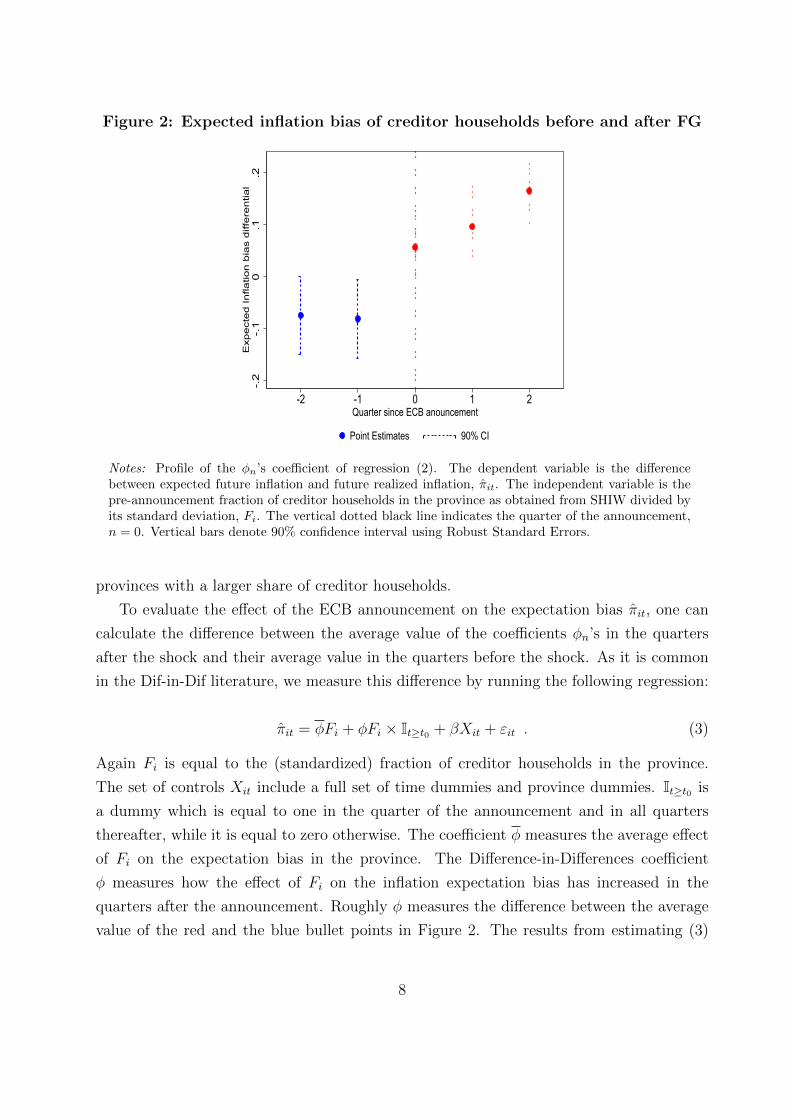
Figure 2: Expected inflation bias of creditor households before and after FG

-.2

-.1

0.1

.2E

xpe

cte

d I

nfla

tion

bia

s d

iffe

ren

tial

-2 -1 0 1 2Quarter since ECB anouncement

Point Estimates 90% CI

Notes: Profile of the φn’s coefficient of regression (2). The dependent variable is the differencebetween expected future inflation and future realized inflation, πit. The independent variable is thepre-announcement fraction of creditor households in the province as obtained from SHIW divided byits standard deviation, Fi. The vertical dotted black line indicates the quarter of the announcement,n = 0. Vertical bars denote 90% confidence interval using Robust Standard Errors.

provinces with a larger share of creditor households.

To evaluate the effect of the ECB announcement on the expectation bias πit, one can

calculate the difference between the average value of the coefficients φn’s in the quarters

after the shock and their average value in the quarters before the shock. As it is common

in the Dif-in-Dif literature, we measure this difference by running the following regression:

πit = φFi + φFi × It≥t0 + βXit + εit . (3)

Again Fi is equal to the (standardized) fraction of creditor households in the province.

The set of controls Xit include a full set of time dummies and province dummies. It≥t0 is

a dummy which is equal to one in the quarter of the announcement and in all quarters

thereafter, while it is equal to zero otherwise. The coefficient φ measures the average effect

of Fi on the expectation bias in the province. The Difference-in-Differences coefficient

φ measures how the effect of Fi on the inflation expectation bias has increased in the

quarters after the announcement. Roughly φ measures the difference between the average

value of the red and the blue bullet points in Figure 2. The results from estimating (3)

8

are reported in Table 2. Column 1 refers to the specification with no province fixed effects,

column 2 reports the results after controlling for a full set of province level dummies.

The estimates indicate that, after the ECB announcement, provinces with a one-standard-

deviation higher share of creditor households have experienced a relative increase in their

inflation expectation bias of around 9 basis points.

Table 2: Effects of FG on the expected inflation bias of creditor households

VARIABLES (1) (2)

Fraction of creditors, Fi, (coefficient φ) -0.02 -0.23(0.03) (0.15)

Announcement-dummy × Fi, (coefficient φ) 0.09∗∗∗ 0.09∗∗∗

(0.03) (0.03)

R2 0.35 0.49N. of observations 1078 1078N. of provinces 108 108

Year FE Y YProvince FE N Y

Notes: Results from running regression (3). All regressions include year fixed effect. The dependentvariable is πit as defined in (3). The sample period is 2012:I-2014:II. Fi is the (standardized) pre-announcement fraction of households with positive NFA in the province. Robust standard errorsin parentheses. *** p<0.01, ** p<0.05, * p<0.10.

3 The model

We start considering a simple economy in discrete time, which we extend in Section 5 for a

quantitative analysis. The economy is populated by a unit mass of households, indexed by

x ∈ [0, 1], who are ambiguity averse and just differ in their net financial wealth, axt ∈ [at, at],

invested in one-period bonds. There is a unit mass of firms that demand labor to produce

intermediate goods sold under a regime of monopolistic competition and prices are sticky.

The nominal interest rate is continuously adjusted to achieve the inflation target set by

a monetary authority with an unambiguous mandate of price stability. The monetary

authority has always complied with its mandate by fully stabilizing prices over the history

of the economy. We focus the analysis on the short run response of the economy, after the

monetary authority, suddenly and unexpectedly, announces a future change in the inflation

9

target, which makes households doubt whether the authority will actually deviate from its

historical mandate as announced. Hereafter we adopt the convention that, unless otherwise

specified, variables are real—measured in units of the final consumption good.

Households Household x ∈ [0, 1] is infinitely lived, with a subjective discount factor

β < 1 and per period preferences over consumption cxt and labor lxt given by

U(cxt, lxt) =

(cxt − ψ0

l1+ψxt

1+ψ

)1−σ

1− σ, (4)

with ψ0, ψ > 0 and σ ≥ 1. When all households share the same beliefs, these preferences

(Greenwood, Hercowitz, and Huffman 1988) guarantee that the economy features a rep-

resentative household, which is a canonical benchmark in the New Keynesian literature.

Financial markets are incomplete, in that households can invest just in a one-period bond,

which, at time t, pays (gross) return rt per unit invested.2 Households can freely borrow by

going short in the asset. The labor market is perfectly competitive, so households take the

wage wt as given. At each point in time t, household-x chooses the triple cxt, lxt, axt+1subject to the budget constraint

cxt + axt+1 ≤ wt lxt + rt axt + λt , (5)

where axt+1 measures the units invested in bonds at time t which will yield return rt+1 at

time t+ 1, while λt denotes (lump sum) government transfers (specified below).

Monetary policy rule The monetary authority sets the (gross) nominal interest rate

Rt+1 between time t and t+ 1 (paid in t+ 1) according to

Rt+1

R=

(Πt

Π∗t

)(1−ρr)φ (Rt

R

)ρr, (6)

where φ > 1 and ρr ∈ [0, 1), R is the steady state interest rate, Πt ≡ pt/pt−1 is gross

inflation, and Π∗t is the time-t inflation target, which is equal to one in steady state, Π∗ = 1.

Firms The final consumption good is produced by a (representative) competitive firm,

which uses a continuum of varieties i ∈ [0, 1] as inputs according to

Yt =

(∫ 1

0

yθ−1θ

it di

) θθ−1

, (7)

2In Appendix C.1, we consider an extension with long-term bonds.

10

where yit is the amount of variety i used in production. The variety i is produced only by a

firm i which uses a linear-in-labor production function, so that yit = `it, where `it denotes

firm-i labor demand, whose unitary cost is wt. Firm i ∈ [0, 1] sets the nominal price for

its variety pit to maximize the beginning of period expected profits, dit ≡ yit (pit/pt − wt),taking as given the demand schedule by the competitive firm, the aggregate nominal price,

pt, and the wage rate, wt. We assume firm i chooses its nominal price at time t, pit, after the

monetary authority has set the inflation target for that period Π∗t (but before any time-t

policy announcement). Finally, we start assuming that the government owns all firms in

the economy and rebates all profits back to households in a lump-sum fashion, so that

λt =∫ 1

0dit di. We relax this assumption in Section 5.

Markets clearing In equilibrium, output Yt is equal to aggregate consumption Ct ≡∫ 1

0cxt dx, so that Yt = Ct, and labor demand is equal to labor supply,

∫ 1

0`itdi =

∫ 1

0lxtdx.

Since bonds are in zero net supply, clearing of the financial market requires that∫ 1

0ax,t = 0

at the return rt = Rt/Πt, where the nominal interest rate Rt satisfies (6).

Steady state At t = 0, the economy is initially in a steady state, where a monetary

authority with an unambiguous mandate of price stability has always set Π∗t = 1, and

households expect Π∗t to remain equal to one also in the future ∀t, implying r = R = 1/β

and Π = 1, where an upper-bar denotes the steady state value of the corresponding quantity.

Policy announcement At t = 0, (and after firms have set their nominal price), the

monetary authority announces that in period T > 0, and only at T , the inflation target will

deviate from full price stability, implying that Π∗T = ε, and Π∗t = 1 for all t 6= T . If ε > 1,

the announcement is inflationary ; if ε < 1, it is deflationary. Given the announcement,

household x ∈ [0, 1] makes her consumption, labor supply and saving decisions, while firms

i ∈ [0, 1] supplies any amount demanded at their (previously) set price.

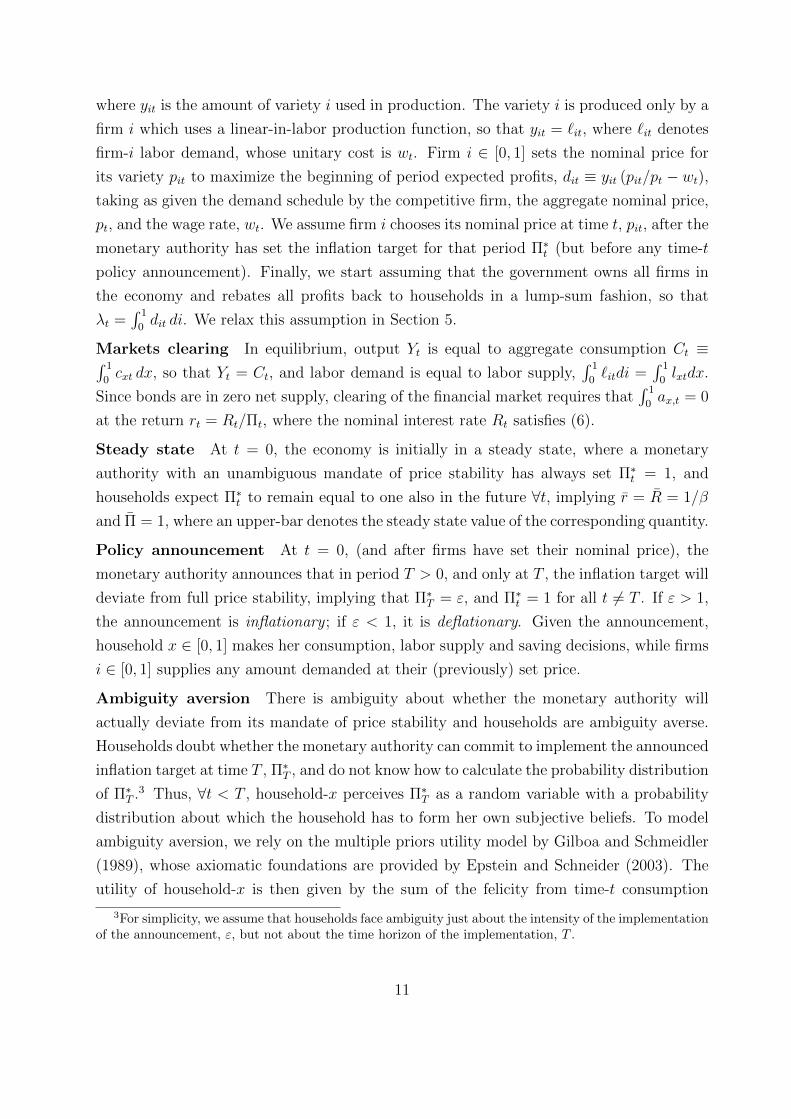
Ambiguity aversion There is ambiguity about whether the monetary authority will

actually deviate from its mandate of price stability and households are ambiguity averse.

Households doubt whether the monetary authority can commit to implement the announced

inflation target at time T , Π∗T , and do not know how to calculate the probability distribution

of Π∗T .3 Thus, ∀t < T , household-x perceives Π∗T as a random variable with a probability

distribution about which the household has to form her own subjective beliefs. To model

ambiguity aversion, we rely on the multiple priors utility model by Gilboa and Schmeidler

(1989), whose axiomatic foundations are provided by Epstein and Schneider (2003). The

utility of household-x is then given by the sum of the felicity from time-t consumption

3For simplicity, we assume that households face ambiguity just about the intensity of the implementationof the announcement, ε, but not about the time horizon of the implementation, T .

11

and labor plus the expected continuation utility, which is evaluated under the household-

x worst-case scenario about the future realizations of the inflation target. Formally, we

assume that preferences at time t order future streams of consumption, Ct = cs(hs)∞s=t,and labor supply, Lt = ls(hs)∞s=t, so that utility is defined recursively as follows:

Vt(Ct,Lt) = U(ct, lt) + β minΩ⊆St, G∈P(Ω)

∫Ω

Vt+1(Ct+1,Lt+1)G(dΠ∗t+1) , (8)

where ht = Π∗−∞, ...,Π∗t−1,Π∗t denotes the history up to time t, Ω is the support of the

probability distribution G that household x associates to the realizations of the inflation

target one period ahead, Π∗t+1. Expected utility arises when the household is forced to take

Ω and the associated probability distribution G as given. Under ambiguity aversion, to

rank the utility from future streams of consumption and labor, the household chooses a

support Ω and an associated probability distribution G so as to minimize the continuation

utility Vt+1 (worst case criterion). The support Ω is chosen among the possible realizations

of the inflation target in t + 1, which is denoted by St. A non-degenerate set of beliefs

captures the household’s lack of confidence in probability assessments, with a larger set

implying greater ambiguity about the future. The probability distribution G is chosen in

the set of all probability distributions P(Ω) that assign positive probability to all values in

the support Ω. We assume that, ∀t, household x ∈ [0, 1] can condition her choices to the

entire history up to time t, ht, which is fully characterized by the observed realizations of

Π∗t up to t. Household x chooses her consumption plans, ct(ht), her labor supply lt(h

t) and

her savings at+1(ht) so as to maximize (8). Notice that, if the realizations of the inflation

target affect the consumption and labor streams of different households differently, these

preferences will give rise to actions that are taken under heterogeneous beliefs.

In our experiment, the household faces ambiguity about the realization of Π∗T only,

so the set St is non-degenerate just at t = T − 1. In particular, we assume that ST−1 =

[minε, 1,maxε, 1]: when the announcement is inflationary, ε > 1, we have ST−1 = [1, ε];

when it is deflationary, ε < 1, we have ST−1 = [ε, 1]. The motivation for this specification

is that a monetary authority with a mandate of price stability, which has been maintained

successfully over a long past history, makes household-x doubt whether the central bank

will actually deviate from its mandate as announced and, if so, by how much.4 There is no

ambiguity about the inflation target pursued by the monetary authority at t < T − 1 or at

t ≥ T . So we have St = 1 ∀t 6= T − 1. Finally, notice that, since the set St is common to

4As it will become clear from the analysis below, this is a conservative assumption because any largersupport implies more heterogeneity in equilibrium households’ beliefs, which would generally strengthenour results.

12

all households x ∈ [0, 1], they all face the same amount of ambiguity.5 We can now define

an equilibrium as follows:

Equilibrium An equilibrium is a set of beliefs, quantities, and prices such that, ∀t,

1. Each household x ∈ [0, 1] chooses cxt, lxt, and axt+1 to maximize the utility in (8),

which also determines her beliefs about the support for the next period realizations of

the inflation target, Ωx ⊆ St, and the associated probability distribution Gx ∈ P(St);

2. The monetary authority sets the nominal interest rate Rt as in (6);

3. Each firm i ∈ [0, 1] sets the price pit = pt optimally, after the inflation target for the

period has been determined (but before any policy announcement);

4. The labor market, the goods markets, and the financial market all clear at the wage

wt, the inflation Πt, and the return rt.

4 Model solution

We start assuming that the policy announcement at t = 0 is about the next-period inflation

target Π∗1, so that T = 1. We also assume that there are only two types of households who

differ just in their initial financial wealth.6 A fraction one half of households is a creditor,

j = c, with wealth equal to ax0 = ac0 = B > 0 ∀x ∈ [0, 1/2], while the remaining fraction

is a debtor, j = d, with financial wealth ax0 = ad0 = −B < 0, ∀x ∈ [1/2, 1]. Here B

denotes the amount of initial financial imbalances in the economy. We start proving two

simple results that clarify the functioning of the model. Then we solve for the equilibrium

by proceeding in three steps: we first determine the allocation of the economy for given

households’ degenerate beliefs about Π∗1; we endogenize beliefs by using (8); and finally we

fully characterize the equilibrium.

5There is empirical evidence suggesting that more educated individuals and those with greater finan-cial literacy are characterized by smaller ambiguity when investing in financial markets and dealing withfinancial institutions, see Dimmock, Kouwenberg, Mitchell, and Peijnenburg (2016). Here we do not allowfor exogenous differences in ambiguity to better isolate the effects of wealth inequality on the formation ofhouseholds’ expectations, which endogenously generate heterogeneity in beliefs.

6Both assumptions are relaxed in the quantitative model of Section 5. To keep the notation consistentthroughout the paper, we have described the economy for general T and for an arbitrary distributionof households’ assets axt. In this simple model the assumption T = 1 is with minor loss of generality,because firms adjust prices in every period so output can respond just at t = 0. The time horizon of theannouncement will matter in the quantitative model because prices are slowly adjusted.

13

4.1 Two preliminary results

Figure 3 describes the time line of the experiment. At the time of the announcement, t = 0,

prices are predetermined at a value normalized to one, p0 = 1. The focus of the analysis is

in characterizing output at time zero, Y0 which, given sticky prices, is determined by the

saving decisions of creditors, ac1, and debtors, ad1. Clearing of the financial market implies

that ac1 = −ad1 = B′, where B′ denotes the amount of financial imbalances at the end of

period zero. In the following periods, t ≥ 1, firm i ∈ [0, 1] sets its price pit to maximize

expected profits at the beginning of period, dit ≡ yit (pit/pt−wt), after taking as given the

demand for the variety of the competitive firm, which has the conventional form:

yit = Yt

(pitpt

)−θ.

The resulting optimal nominal price is a markup over firm-i expected nominal wage:

pit =θ

θ − 1Eit[wt pt] ∀i ∈ [0, 1], (9)

which immediately implies pit = pt ∀i. Also, since firms set their price after observing Π∗t ,

firms choices are taken under perfect information ∀t ≥ 1, which allow us to conclude that

wt =θ − 1

θ, ∀t ≥ 1. (10)

The utility in (4) together with the preferences in (8) also imply that the labor supply of

a household of type j = c, d solves a simple static maximization problem, which yields the

familiar condition

ψ0 lψjt = wt. (11)

This implies that all households supply the same labor (independently of their wealth and

their beliefs): ljt = Yt, ∀j, which uses the fact that, in equilibrium, labor supply equals

output. The latter, together with (10) and (11), immediately implies that:

Lemma 1 Output Yt converges back to steady state at t = 1, so that Yt = Y for all t ≥ 1.

Moreover Lemma 1 together with the interest rate rule in (6) allows us to prove that

Lemma 2 At any point in time t ≥ 0, the inflation is equal to the inflation target, Πt = Π∗t ,

and the nominal interest remains unchanged at its steady state value, Rt = R.

Proof of Lemma 2. R0 = R because the economy is initially in a steady state. Given

the timing of the monetary announcement, prices do not respond at t = 0 so Π0 = Π∗0 = 1,

14

which after using (6) yields R1 = R. Lemma 1 implies that the economy is back to steady

state starting from t = 1 so it must be that rt = R ∀t ≥ 2 (which obviously follows from the

Euler equation of consumption below). By assumption we also have Πt = Π∗t = 1, ∀t ≥ 2

so we have Rt = rt = R ∀t ≥ 2, which immediately allows us to conclude that Rt = R ∀t.But this together with (6) also implies that Πt = Π∗t ∀t ≥ 0.

In Section 5 we consider an extension of the model where changes in the inflation target

also affect nominal interest rates.7

Figure 3: Timing

p0 = 1

Π∗0 = 1

R0 = R

t = 0−

AnnouncementHHs form beliefs

Y0 and B′

t = 0 t=1

Y1 = YR1 = RΠ1 = Π∗1r1 = R/Π∗1

t ≥ 2

Yt = YRt = RΠt = 1rt = R

4.2 Output and the financial market for given beliefs

We now assume that a household j = c, d has given degenerate beliefs about the realization

of Π∗1, which are represented by a point ετj ∈ S0 with τj ∈ [0, 1]. In practice it is useful

to define τ ≡ (τc + τd)/2 and ρ ≡ (τc − τd)/(2τ) ∈ [−1, 1], which are related to τc and

τd as follows: τc ≡ τ (1 + ρ) and τd ≡ τ (1 − ρ). τ measures the average credibility of

the announcement among all households in the economy; while ρ measures the correlation

between the financial asset position of households and their perceived credibility of the

announcement. When ρ > 0, creditors believe the announcement more than debtors do,

while the opposite is true when ρ < 0; ρ = 0 means that all households share the same

beliefs. The problem of a household of type j = c, d at t = 0 is then given by

maxcjs,ljs,ajs+1s≥0

Ej0

[∞∑s=0

βs U(cjs, ljs)

],

subject to the budget constraint in (5). The expectation operator is indexed by j, since

households of different types (might) have different beliefs. The first order condition for

7But the result that nominal interest rates do not move mimics a situation where nominal rates cannotmove (say because they have hit the zero lower bound) and the monetary authority tries to stimulate theeconomy in the short run through promises of higher future inflation, by announcing that current nominalrates will remain low for an extended period of time.

15

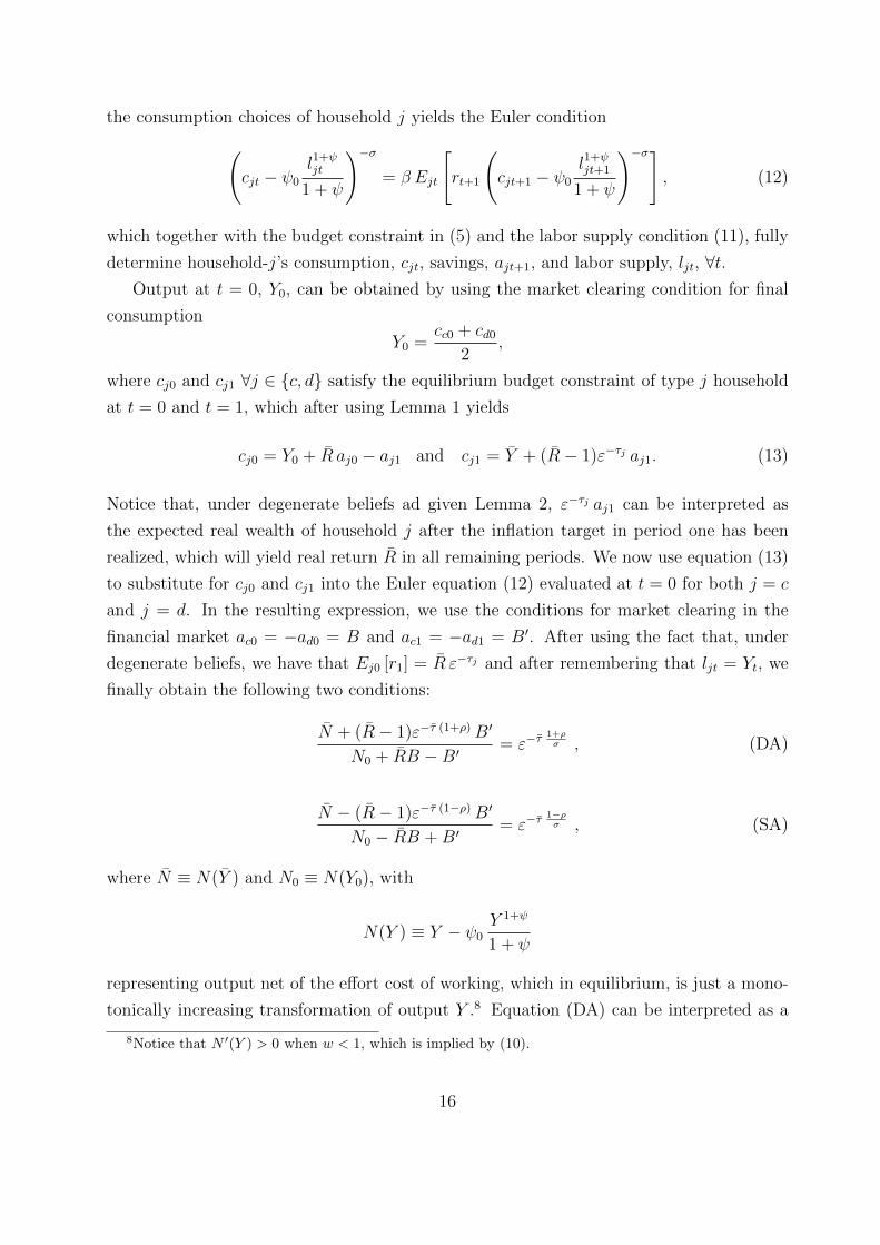
the consumption choices of household j yields the Euler condition(cjt − ψ0

l1+ψjt

1 + ψ

)−σ= β Ejt

[rt+1

(cjt+1 − ψ0

l1+ψjt+1

1 + ψ

)−σ], (12)

which together with the budget constraint in (5) and the labor supply condition (11), fully

determine household-j’s consumption, cjt, savings, ajt+1, and labor supply, ljt, ∀t.Output at t = 0, Y0, can be obtained by using the market clearing condition for final

consumption

Y0 =cc0 + cd0

2,

where cj0 and cj1 ∀j ∈ c, d satisfy the equilibrium budget constraint of type j household

at t = 0 and t = 1, which after using Lemma 1 yields

cj0 = Y0 + R aj0 − aj1 and cj1 = Y + (R− 1)ε−τj aj1. (13)

Notice that, under degenerate beliefs ad given Lemma 2, ε−τj aj1 can be interpreted as

the expected real wealth of household j after the inflation target in period one has been

realized, which will yield real return R in all remaining periods. We now use equation (13)

to substitute for cj0 and cj1 into the Euler equation (12) evaluated at t = 0 for both j = c

and j = d. In the resulting expression, we use the conditions for market clearing in the

financial market ac0 = −ad0 = B and ac1 = −ad1 = B′. After using the fact that, under

degenerate beliefs, we have that Ej0 [r1] = R ε−τj and after remembering that ljt = Yt, we

finally obtain the following two conditions:

N + (R− 1)ε−τ (1+ρ) B′

N0 + RB −B′= ε−τ

1+ρσ , (DA)

N − (R− 1)ε−τ (1−ρ) B′

N0 − RB +B′= ε−τ

1−ρσ , (SA)

where N ≡ N(Y ) and N0 ≡ N(Y0), with

N(Y ) ≡ Y − ψ0Y 1+ψ

1 + ψ

representing output net of the effort cost of working, which in equilibrium, is just a mono-

tonically increasing transformation of output Y .8 Equation (DA) can be interpreted as a

8Notice that N ′(Y ) > 0 when w < 1, which is implied by (10).

16

demand for assets by creditors: by the consumption smoothing motive, the demand for

assets of creditors is increasing in time-zero net output, N0, because households want to

save more when output temporarily increases. This corresponds to the positively sloped

straight blue line in Figure 4. By the same logic, equation (SA) can be interpreted as char-

acterizing the supply of assets by debtors: the supply of assets in the economy is decreasing

in the level of output at t = 0 as debtors want to borrow less (save more) when time-zero

output is higher. This corresponds to the negatively sloped straight red line in Figure 4.

The financial market clears at the point where the two schedules cross, which is unique and

corresponds to point A in the Figure. The associated value of time-zero net output N0, is

obtained by combining (DA) with (SA) to obtain

N0 = N0(ε, τ , ρ) ≡ N(ω ε

1+ρσ + (1− ω) ε

1−ρσ

)+B κ

(ε (1+ρ) ( 1

σ−1) − ε (1−ρ) ( 1

σ−1)), (14)

where ε ≡ ε τ measures the announcement rescaled by its average credibility while

ω ≡ 1 + (R− 1) ε (1−ρ) ( 1σ−1)

2 + R−12

(ε (1+ρ) ( 1

σ−1) + ε (1−ρ) ( 1

σ−1)) ∈ [0, 1] ,

κ ≡ R (R− 1)

2 + (R− 1)[ε (1+ρ) ( 1

σ−1) + ε (1−ρ) ( 1

σ−1)] > 0.

We can summarize this discussion by stating the following Lemma:

Lemma 3 When the beliefs of households are given and degenerate, as characterized by

τ ∈ [0, 1] and ρ ∈ [−1, 1], net output N0 and financial imbalances B′ are determined by

the point where the demand for assets (DA) and the supply of assets (SA) cross. The

intersection is unique and the resulting N0 is given by the function N0(ε, τ , ρ) in (14).

The first term in the right hand side of (14) is always positive and characterizes how

aggregate consumption is affected by the substitution effect, implied by temporary changes

in the expected real rate. The second term in the right hand side of (14) can be positive

or negative and characterizes the effects on consumption of redistributing future expected

wealth from one household type to the other. This term is zero, when B = 0 because

there is no wealth redistribution. It also zero when ρ = 0, because in this case the wealth

losses expected by the type of household who looses (creditors when ε > 1, debtors when

ε < 1) are identical to the wealth gains expected by the other type. And zero-sum transfers

of wealth from one household’s type to the other have no effects on consumption because

all households share the same marginal propensity to consume—due to both the utility

function in (4) and the absence of financial constraints. So when B = 0 or when ρ = 0, net

17

output is equal to N0 = ε1σ N , as in a standard New Keynesian model with a representative

household where the announcement is just scaled down by its average credibility ε = ε τ .

The canonical New Keynesian benchmark model, where all households in the economy fully

believe the announcement, arises when τ = 1 and ρ = 0. By substituting these values into

(14), we immediately obtain that N0 = ε1σ N , which can be substituted back into (DA) to

solve for B′ so as to obtain

B′ =R B

1 + (R− 1) ε1σ−1,

which also implies that the new steady state imbalances that result once the announcement

is implemented are equal toB′

ε=

R

Rε1σ + ε− ε 1

σ

B.

Under σ > 1 we immediately see that B′/ε− B < 0 if ε > 1, while B′/ε− B > 0 if ε < 1,

which leads to the following Proposition:

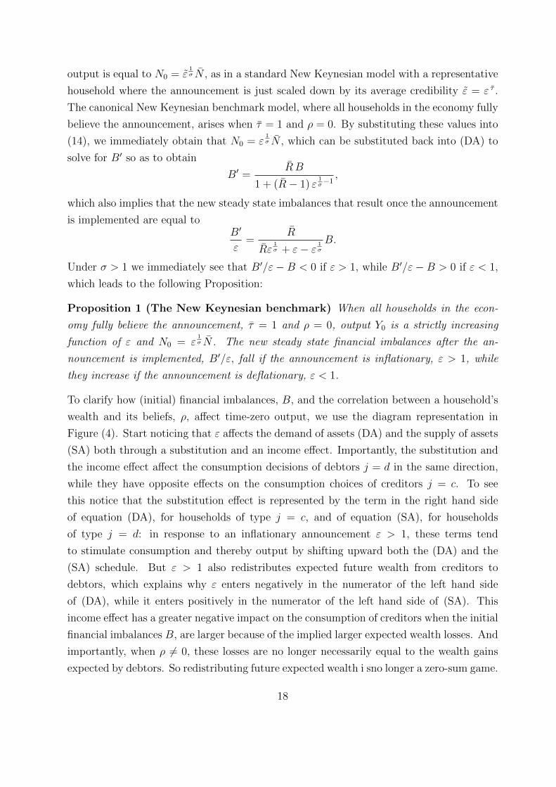
Proposition 1 (The New Keynesian benchmark) When all households in the econ-

omy fully believe the announcement, τ = 1 and ρ = 0, output Y0 is a strictly increasing

function of ε and N0 = ε1σ N . The new steady state financial imbalances after the an-

nouncement is implemented, B′/ε, fall if the announcement is inflationary, ε > 1, while

they increase if the announcement is deflationary, ε < 1.

To clarify how (initial) financial imbalances, B, and the correlation between a household’s

wealth and its beliefs, ρ, affect time-zero output, we use the diagram representation in

Figure (4). Start noticing that ε affects the demand of assets (DA) and the supply of assets

(SA) both through a substitution and an income effect. Importantly, the substitution and

the income effect affect the consumption decisions of debtors j = d in the same direction,

while they have opposite effects on the consumption choices of creditors j = c. To see

this notice that the substitution effect is represented by the term in the right hand side

of equation (DA), for households of type j = c, and of equation (SA), for households

of type j = d: in response to an inflationary announcement ε > 1, these terms tend

to stimulate consumption and thereby output by shifting upward both the (DA) and the

(SA) schedule. But ε > 1 also redistributes expected future wealth from creditors to

debtors, which explains why ε enters negatively in the numerator of the left hand side

of (DA), while it enters positively in the numerator of the left hand side of (SA). This

income effect has a greater negative impact on the consumption of creditors when the initial

financial imbalances B, are larger because of the implied larger expected wealth losses. And

importantly, when ρ 6= 0, these losses are no longer necessarily equal to the wealth gains

expected by debtors. So redistributing future expected wealth i sno longer a zero-sum game.

18

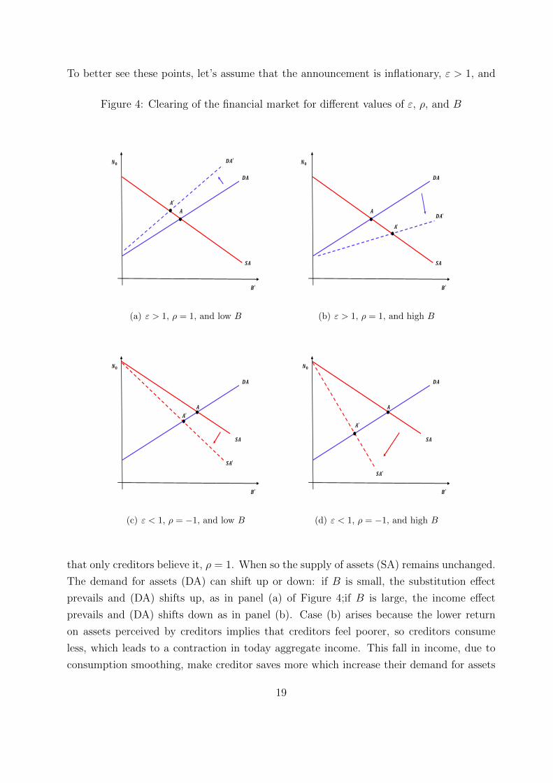
To better see these points, let’s assume that the announcement is inflationary, ε > 1, and

Figure 4: Clearing of the financial market for different values of ε, ρ, and B

(a) ε > 1, ρ = 1, and low B

(b) ε > 1, ρ = 1, and high B

(c) ε < 1, ρ = −1, and low B

(d) ε < 1, ρ = −1, and high B

that only creditors believe it, ρ = 1. When so the supply of assets (SA) remains unchanged.

The demand for assets (DA) can shift up or down: if B is small, the substitution effect

prevails and (DA) shifts up, as in panel (a) of Figure 4;if B is large, the income effect

prevails and (DA) shifts down as in panel (b). Case (b) arises because the lower return

on assets perceived by creditors implies that creditors feel poorer, so creditors consume

less, which leads to a contraction in today aggregate income. This fall in income, due to

consumption smoothing, make creditor saves more which increase their demand for assets

19

and allows the financial market to clear even if the real rate on assets expected by debtors

has remained unchanged.

Things are different when focusing on debtors, because for them the income and sub-

stitution effect work in the same direction. Panel (c) and (d) of Figure 4 illustrate this

point by focusing on a deflationary announcement ε < 1 that is believed just by debtors,

rho = −1. In this case, (DA) remains unchanged, while the supply of assets SA always

move down, the more so the larger is B. And as debtors borrow less, their consumption

and thereby aggregate output fall which allow to restore equilibrium in the financial market

by reducing the demand for assets of creditors, at their given expected return on assets.

The next proposition summarizes this discussion:

Proposition 2 (Output with heterogeneous beliefs) For given households beliefs, as

characterized by τ ∈ [0, 1] and ρ ∈ [−1, 1], net output N0 is given by the function N0(ε, τ , ρ)

in (14), which implies that

1. If ρ > 0, greater initial imbalances, B, reduce the response of time-zero output Y0 to

inflationary announcement, ε > 1. And if they are large enough, Y0 contracts;

2. When ρ < 0, Y0 always falls in response to a deflationary announcement, ε < 1. And

more so when initial imbalances, B, are larger.

Numerical illustration In Figure 5 we plot the response of output to a 1% inflationary

announcement for different parameter values. The blue solid line in each plot uses the

parameter values of Table 3 when ρ = 1 and τ = 1/2—which will turn out to be the

equilibrium beliefs. B is set equal to the standard deviation of the ratio of wealth to

yearly labor income in the Euro Area. We discuss the effects of changing ρ in panel (a); of

changing B, in panel (b); and of changing σ in panel (c). The lower the correlation between

the wealth of households and their perceived credibility of the inflationary announcement,

the larger is the output response: it increases from -0.3% of steady state under ρ = 1 to a

110% increase of steady state when ρ = −1. Panel (b) shows how smaller imbalances, leads

to larger increases in output: when B = 0 output increase by 0.4% of steady state output

as compared to the the fall of 0.3% under the baseline specification. Panel (c) shows how

a higher Elasticity of Intertemporal Substitution (smaller σ) leads to a a larger increase in

output.

4.3 Endogenous beliefs

We now characterize how households form their beliefs about the likelihood and magnitude

of the future change in the inflation target Π∗1. Since by Lemma 1 the economy is back to

20

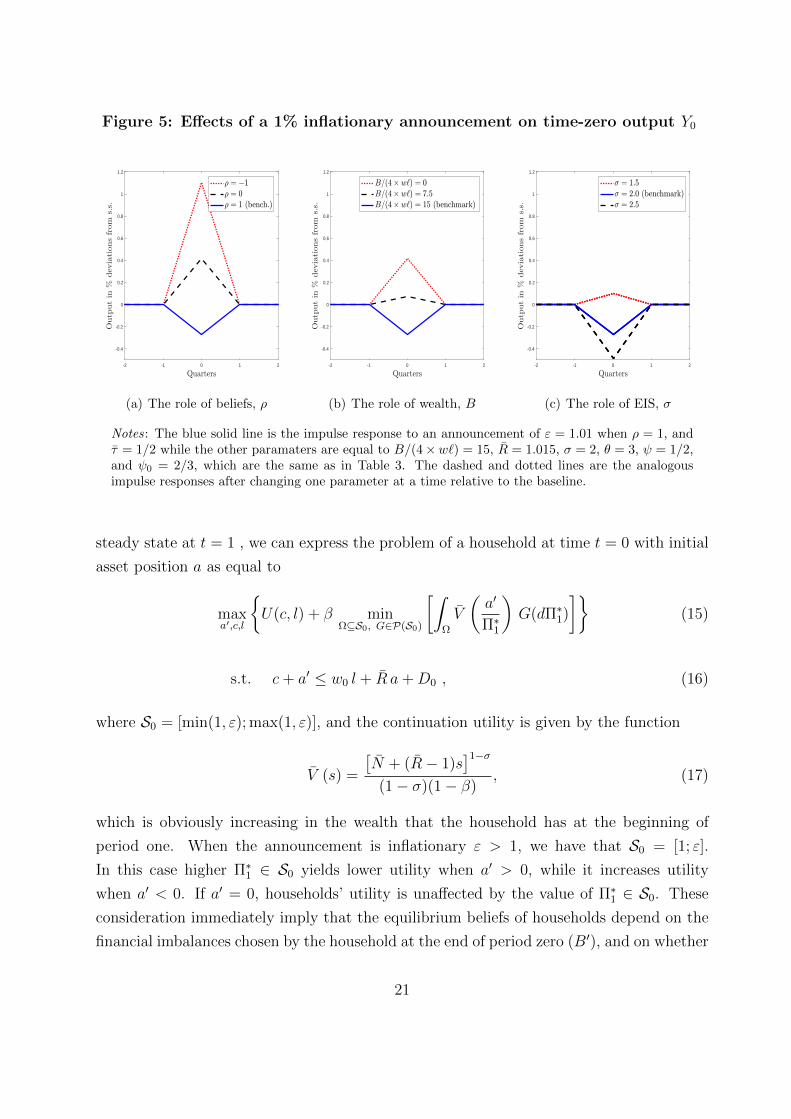
Figure 5: Effects of a 1% inflationary announcement on time-zero output Y0

-2 -1 0 1 2

Quarters

-0.4

-0.2

0

0.2

0.4

0.6

0.8

1

1.2

Outp

utin

%devia

tionsfrom

s.s.

; = !1; = 0; = 1 (bench.)

(a) The role of beliefs, ρ

-2 -1 0 1 2

Quarters

-0.4

-0.2

0

0.2

0.4

0.6

0.8

1

1.2

Outp

utin

%devia

tionsfrom

s.s.

B=(4# w`) = 0B=(4# w`) = 7:5B=(4# w`) = 15 (benchmark)

(b) The role of wealth, B

-2 -1 0 1 2

Quarters

-0.4

-0.2

0

0.2

0.4

0.6

0.8

1

1.2

Outp

utin

%devia

tionsfrom

s.s.

< = 1:5< = 2:0 (benchmark)< = 2:5

(c) The role of EIS, σ

Notes: The blue solid line is the impulse response to an announcement of ε = 1.01 when ρ = 1, andτ = 1/2 while the other paramaters are equal to B/(4×w`) = 15, R = 1.015, σ = 2, θ = 3, ψ = 1/2,and ψ0 = 2/3, which are the same as in Table 3. The dashed and dotted lines are the analogousimpulse responses after changing one parameter at a time relative to the baseline.

steady state at t = 1 , we can express the problem of a household at time t = 0 with initial

asset position a as equal to

maxa′,c,l

U(c, l) + β min

Ω⊆S0, G∈P(S0)

[∫Ω

V

(a′

Π∗1

)G(dΠ∗1)

](15)

s.t. c+ a′ ≤ w0 l + R a+D0 , (16)

where S0 = [min(1, ε); max(1, ε)], and the continuation utility is given by the function

V (s) =

[N + (R− 1)s

]1−σ(1− σ)(1− β)

, (17)

which is obviously increasing in the wealth that the household has at the beginning of

period one. When the announcement is inflationary ε > 1, we have that S0 = [1; ε].

In this case higher Π∗1 ∈ S0 yields lower utility when a′ > 0, while it increases utility

when a′ < 0. If a′ = 0, households’ utility is unaffected by the value of Π∗1 ∈ S0. These

consideration immediately imply that the equilibrium beliefs of households depend on the

financial imbalances chosen by the household at the end of period zero (B′), and on whether

21

the announcement is inflationary ε > 1 or deflationary ε < 1. In brief we have that:

Proposition 3 (Individual beliefs) A household’s beliefs depend of the announcement,

ε, and of the household’s end-of period savings, a′. When a′ = 0 beliefs are undeterminate.

If a′ 6= 0 they are always degenerate and equal to ετ(a′,ε) where

τ(a′, ε) = I(ε > 1)× I(a′ > 0) + I(ε < 1)× I(a′ < 0), (18)

where I denotes the indicator function.

If households have no savings at the end period t = 0, a′ = 0, the beliefs of the household are

undeterminate because the household is indifferent about any future choices of the monetary

authority. Figure 6 characterizes the beliefs of households as a function of the end-of-period

financial imbalances chosen by the household, a′ > 0, and of the nature of the announcement

ε. The function τ(a′, ε) measures the percentage amount of the announcement ε that the

household thinks the monetary authority will implement in period one. If the announcement

is inflationary, ε > 1, τ(a′, ε) = 1 if a′ > 0 and zero otherwise, which corresponds to panel

(a) of Figure 6. If the announcement is deflationary, ε < 1, τ(a′, ε) = 1 if a′ < 0 while it is

zero otherwise, which corresponds to panel (b).

Figure 6: Endogenous determination of beliefs for ε < 1 and ε > 1

τ(a’)

0

(a) Case ε > 1

=0

τ(a’)

(b) Case ε < 1

22

4.4 Equilibrium

We now characterize the equilibrium beliefs, time-zero output and the new steady state

financial imbalances that emerges at t ≥ 1 when the announcement is actually implemented.

The next proposition characterizes the mapping from financial imbalances at the beginning

of t = 0, B, with imbalances at the end of the period, B′.

Proposition 4 (No reversal in households’ NFA) In equilibrium, creditors and debtors

never switch their net financial asset position, i.e. if B > 0, then B′ ≥ 0.

Proof of Proposition 4. Assume that ε > 1 (similar logic applies when ε < 1) and

argue by contradiction. Suppose that B > 0 leads to B′ < 0. Then, (18) implies that

households of type j = c do not believe the announcement and think that the expected real

rate is unchanged at its steady state level R = 1/β. Then households of type j = c find

optimal to dissave (reduce wealth from B to B′ < 0) only if we have Y0 < Y . But in an

equilibrium with B′ < 0, it also follows from (18) that households of type j = d do believe

the announcement and thereby expect a low return. Then households of type j = d would

find optimal to save (move from a debtor position of B to a creditor position of −B′ > 0)

only if Y0 > Y , which immediately leads to a contradiction.

By combining Proposition 3 and 4 we immediately obtain a characterization of the

aggregate equilibrium beliefs in trems of τ and ρ:

Proposition 5 (Aggregate beliefs) In a credit crunch equilibrium, B′ = 0, households’

beliefs are undeterminate. Otherwise, B′ > 0, only one household’s type believes the an-

nouncement, τ = 1/2: if the announcement is inflationary, ε > 1, creditors believe it,

ρ = 1; if it is deflationary, ε < 1, debtors believe it, ρ = −1. So we generally have

ρ = ρ(ε) ≡ 1− 2I(ε < 1), (19)

where I denotes the indicator function.

If there is a credit crunch, B′ = 0, the beliefs of all households in the economy are unde-

terminate because all households have reached their “peace of mind” and are indifferent

about future choices of the monetary authority. If B′ > 0, instead, equilibrium beliefs are

determinate and degenerate.

We are now able to fully characterize equilibrium output. We calculate the intercept

on the y-axis of the supply of asset by debtors, j = d, and of the demand for assets by

creditors, j = c, both evaluated at the equilibrium beliefs of Proposition 5, so τ = 1/2 and

23

ρ = ρ(ε) as given in (19). The intercept of (SA) is given by

NA0 = min1, ε

1σ N + RB, (20)

while the intercept of (DA) is given by

NB0 = max1, ε

1σ N − RB. (21)

Clearly NB0 < NA

0 is equivalent to

B >|ε 1

σ − 1|N2R

, (22)

which is a necessary and sufficient condition to guarantee that (SA) and (DA) cross at

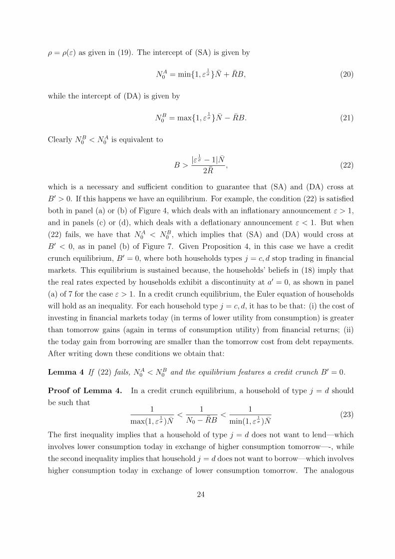
B′ > 0. If this happens we have an equilibrium. For example, the condition (22) is satisfied

both in panel (a) or (b) of Figure 4, which deals with an inflationary announcement ε > 1,

and in panels (c) or (d), which deals with a deflationary announcement ε < 1. But when

(22) fails, we have that NA0 < NB

0 , which implies that (SA) and (DA) would cross at

B′ < 0, as in panel (b) of Figure 7. Given Proposition 4, in this case we have a credit

crunch equilibrium, B′ = 0, where both households types j = c, d stop trading in financial

markets. This equilibrium is sustained because, the households’ beliefs in (18) imply that

the real rates expected by households exhibit a discontinuity at a′ = 0, as shown in panel

(a) of 7 for the case ε > 1. In a credit crunch equilibrium, the Euler equation of households

will hold as an inequality. For each household type j = c, d, it has to be that: (i) the cost of

investing in financial markets today (in terms of lower utility from consumption) is greater

than tomorrow gains (again in terms of consumption utility) from financial returns; (ii)

the today gain from borrowing are smaller than the tomorrow cost from debt repayments.

After writing down these conditions we obtain that:

Lemma 4 If (22) fails, NA0 < NB

0 and the equilibrium features a credit crunch B′ = 0.

Proof of Lemma 4. In a credit crunch equilibrium, a household of type j = d should

be such that1

max(1, ε1σ )N

<1

N0 − RB<

1

min(1, ε1σ )N

(23)

The first inequality implies that a household of type j = d does not want to lend—which

involves lower consumption today in exchange of higher consumption tomorrow—-, while

the second inequality implies that household j = d does not want to borrow—which involves

higher consumption today in exchange of lower consumption tomorrow. The analogous

24

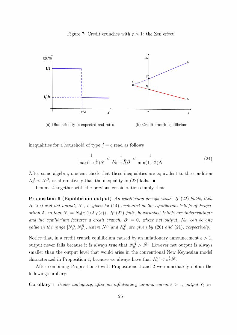
Figure 7: Credit crunches with ε > 1: the Zen effect

E(R/Π)

=0

1/(βε)

1/β

(a) Discontinuity in expected real rates

′

(b) Credit crunch equilibrium

inequalities for a household of type j = c read as follows

1

max(1, ε1σ )N

<1

N0 + RB<

1

min(1, ε1σ )N

(24)

After some algebra, one can check that these inequalities are equivalent to the condition

NA0 < NB

0 , or alternatively that the inequality in (22) fails.

Lemma 4 together with the previous considerations imply that

Proposition 6 (Equilibrium output) An equilibrium always exists. If (22) holds, then

B′ > 0 and net output, N0, is given by (14) evaluated at the equilibrium beliefs of Propo-

sition 5, so that N0 = N0(ε, 1/2, ρ(ε)). If (22) fails, households’ beliefs are indeterminate

and the equilibrium features a credit crunch, B′ = 0, where net output, N0, can be any

value in the range [NA0 , N

B0 ], where NA

0 and NB0 are given by (20) and (21), respectively.

Notice that, in a credit crunch equilibrium caused by an inflationary announcement ε > 1,

output never falls because it is always true that NA0 > N . However net output is always

smaller than the output level that would arise in the conventional New Keynesian model

characterized in Proposition 1, because we always have that NB0 < ε

1σ N .

After combining Proposition 6 with Propositions 1 and 2 we immediately obtain the

following corollary:

Corollary 1 Under ambiguity, after an inflationary announcement ε > 1, output Y0 in-

25

creases less than in the New Keynesian benchmark and it can even fall if B is large enough.

In response to a deflationary announcement, ε < 1, Y0 always falls and more so than in

the New Keynesian benchmark.

Finally we can compare the amount of rebalancing that emerge in our model whence the

announcement is implemented with the corresponding amount of rebalancing that would

emerge in the canonical New Keynesian model where the announcement is fully believed

by all households in the economy:

Proposition 7 (Rebalancing under ambiguity) After an inflationary announcement

ε > 1, the new steady state financial imbalances once the announcement is implemented,

B′/ε, always fall (B′/ε < B), and more so than in the New-Keynesian benchmark. After

a deflationary announcement ε < 1, B′/ε also falls if

B <(1− ε 1

σ )N

2R− (R− 1)(ε1σ − ε)

, (25)

while it always increases in the New-Keynesian benchmark (with ε < 1). Generally, after

any announcement, B′/ε is smaller than the corresponding value in the New-Keynesian

benchmark.

Announcements always generate more rebalancing than in the New Keynesian benchmark

In responses to an inflationary announcement ε > 1, debtors have strong incentives to

deleverage while creditors have little incentive to save because the real rate expected by

creditors is smaller than the real rate expected by debtors, see panel (a) in Figure 7.

This leads to a rebalancing in the financial asset positions of agents and can even cause

credit crunches, which happen because agents stop trading in financial markets so as to get

fully insured against future changes in monetary policy. As a result financial imbalances

naturally fall. Agents naturally reach a level of financial assets that makes them indifferent

about the future choices of monetary policy. This is different from precautionary savings.

Agents naturally tend to obtain a financial position where they reach the peace of mind,

in that their future welfare becomes independent of future monetary policy. This is what

we call the Zen effect. Due to this effect, credit crunches might arise where B′ = 0 even if

B = 0.

5 A quantitative analysis of the forward Guidance announcement by the ECB

In this section we use our framework to study the implications of the Forward Guidance

announcement by the European Central Bank in July 2013 for the Euro area economy.

26

The Euro area is a particularly interesting case to study both because, as we document

later, there was substantial heterogeneity in household wealth at the time of the Forward

Guidance announcement, and because of the evidence we provided in Section 2 about the

relationship between household financial wealth and inflation expectation responses to the

announcement. We model the Euro area as a closed economy populated by households

that differ in net wealth as in Section 3. For simplicity, our analysis abstracts from other

sources of household heterogeneity, such as heterogeneity in production and labor income,

and focuses only on heterogeneity arising from capital income. In order to match key

features of the Euro area economy at the time of the Forward Guidance announcement by

the ECB, we extend the model of Section 3 to allow for persistent responses of output and

inflation to the monetary policy announcement, and for a non zero net supply of financial

assets. We next discuss these extensions in detail.

Sticky prices We assume that firms can adjust prices after the monetary announcement

at t = 0 but face price adjustment costs as in Rotemberg (1982). In particular, we assume

that each intermediate producer chooses its price in each period to maximize profits subject

to price adjustment costs expressed in units of firm output. These adjustment costs are

quadratic in the rate of price change and scaled by aggregate output, Yt:

Θt (πit) =κ

2(πit)

2 Yt , (26)

where πit = (pit − pit−1)/pit−1 is the firm level inflation rate and κ > 0.

Monetary policy experiment As in Section 4, we assume the economy is in steady

state at t = 0, when an announcement is made that the inflation target will stay at its

steady state value, Π∗t = 1, for all t < T , will be equal to Π∗T = ε at t = T . Differently from

before, we allow here for persistence in the deviation of the inflation target from steady

state. In particular, we assume that the inflation target converges back to to its steady state

value according to an AR(1) process, log(Π∗t ) = ρ∗ log(Π∗t−1), for t > T . For simplicity, as in

in Section 4, we assume that household face ambiguity with respect to the implementation

of the policy, but not with respect to its horizon, T , or its persistence, ρ∗. We consider

two cases for the path of the nominal interest rate in the interim periods t ∈ [0, T ). In our

baseline case, we assume that the nominal interest rate will stay constant at its steady state

value, R, for all t ∈ [0, T ), and then be given by equation (6) afterwards. This assumption

mimics the inaction of the policy rate around the forward guidance announcement by the

ECB. In the other case we will instead assume that the nominal interest rate will be given

by equation (6) for all t ≥ 0.

27

Financial market We allow for the supply of financial assets in the economy to be

positive through a competitive mutual fund that owns the firms and is a net debtor with

respect to the households, to which it supplies bonds. The flow budget constraint of the

mutual fund is such that aggregate net payments, rt∫ 1

0axt dx, are balanced by dividends

Dt and new net issuance of bonds,∫ 1

0axt+1 dx, in each period:

rt

∫ 1

0

axt dx+ Υ = Dt +

∫ 1

0

axt+1 dx . (27)

We assume that a value Υ of the overall inflows to the mutual fund is not paid to households,

and interpret it as a payment to hypothetical foreign agents for debt held abroad. We will

use Υ to calibrate the net supply of financial assets in the economy.

5.1 Characterization of the equilibrium

In this section we derive the conditions that determine the equilibrium and discuss its key

properties. Each firm i sets the price pit in period t to solve the following problem

maxpis∞s=t

Eit

[∞∑s=t

qt,s

((pisps− ws

)Yt

(pisps

)−θ−Θs (πis)

)], (28)

where qt,t+j is the real discount factor between periods t and t+j. The expectation operator

is indexed by i to denote the beliefs of firm i about the path of future output, inflation

and real rate. In our baseline specification, we assume that firms fully trust the policy

announcement of the monetary authority and forms beliefs with rational expectations. We

will later consider the alternative assumption where firms don’t believe the announcement

and show that our quantitative results are even stronger. The solution to the firm problem

implies symmetric pricing, pit = pt and πit = πt for all i, and an equation determining the

dynamics of inflation,

1− κ (Πt − 1) Πt + κEit

[qt,t+1 (Πt+1 − 1) Πt+1

Yt+1

Yt

]= θ (1− wt) . (29)

The demand of each variety is equal to aggregate output, Yt. Hence, the aggregate dividend

of firms is given by

Dt =(

1− wt −κ

2π2t

)Yt . (30)

For given path of output Yt, the nominal interest rate Rt, the real wage wt and inflation

Πt are jointly determined by equations (6), (11) and (28), and the real rate is given by

rt = Rt/Πt. Aggregate output is given by the condition for equilibrium in the goods

28

market,

Yt =Ct + Υ

1− κ2π2t

, (31)

where Ct =∫ 1

0cxt dx. Thus, to close the model, we are left to determine aggregate consump-

tion Ct, which we obtain from the solution to the household problem which we next discuss.

We distinguish between the household problem after the resolution of the ambiguity, i.e.

for t ≥ T , and before it, i.e. for t < T .

Aggregate demand at t ≥ T The problem of the household at any t ≥ T is to maximize

the present discounted value of all future utility,∑∞

s=0 βs U(cxt+s, lxt+s), subject to the

intertemporal budget constraint,∑∞

s=0 qt,t+s (cxt+s − wt+s lxt+s) ≤ rt ax,t, under perfect

foresight. Given the perfect foresight, the optimal choice of cxt, lxt, axt+1t≥T is given by

the first order conditions in equations (11)-(12) together with the budget constraint.

Using these equations we next characterize the solution to the household problem for

a given path of ws, πs, rss≥T . Consider the economy at t ≥ T , after ambiguity is re-

solved. For a given sequence of real wages wss≥T , inflation πss≥T , and real interest

rates rss≥T , the aggregate consumption is independent of the distribution of assets and

is given by

Ct =wt

1 + ψ

(wtψ0

) 1ψ0

+ αt

∞∑j=0

qt,t+j

(ψwt+j1 + ψ

(wt+jψ0

) 1ψ0

+Dt+j −Υ

), (32)

where αt =[∑∞

j=0 qt,t+j

(∏js=1 (β rt+s)

1σ

)]−1

. The consumption of household x with wealth

axt is given by

cxt = Ct + αt [rt axt − St] , (33)

where St ≡ Dt + r−1t+1 St+1 is the value of the market portfolio.

Equation (32) shows that aggregate consumption is independent of the distribution of

assets a at t ≥ T . This is because, differently from t < T , there is no relationship between

the wealth and the beliefs, which are now homogeneous. Moreover, there is no wealth

effect on labor supply, so that the distribution of financial assets does not affect labor

supply. Thus, the aggregate economy behaves as a standard representative household new-

Keynesian economy at t ≥ T .

Equation (33) fully characterizes the optimal household behavior of each household.

At t ≥ T , ambiguity on the behavior of the monetary authority is resolved, the nominal

interest rate is determined by equation (6) together with the realized path of Π∗t , and all

agents have perfect foresight and identical beliefs about the path of economic variables.

The deviation of the consumption of a household from the average consumption in the

29

economy depends from the difference between the value of her financial assets, rt axt, and

the value of the market portfolio, St.

The next proposition describes some useful properties of the equilibrium at t ≥ T when

the nominal interest rate is not a state variable of the economy.

Proposition 8 Assume ρr = 0, or alternatively Rt = R for all t ≤ T . Then the equilibrium

dynamics at t < T do not affect the equilibrium dynamics of aggregate variables at t ≥ T ,

e.g. Ytt≥T is independent of Ytt<T . Moreover, if Π∗T = 1, the economy is in steady

state at t = T .

Proposition (8) characterizes the equilibrium of the economy at t ≥ T when there is no

inertia in the interest rate rule (ρr = 0), or when the interest rate has been at its steady

state value at t < T (as we will assume later). In these cases, past economic dynamics do

not affect the equilibrium of the economy at t ≥ T as the distribution of financial assets

is the only state of the economy, which is however is irrelevant for aggregate dynamics as

shown in Proposition 1. An implication of the corollary is that if the policy announcement

is not implemented, Π∗T = 1, then the economy is in steady state at any t ≥ T .

Aggregate demand at t < T We now characterize aggregate demand at t < T , when

households are ambiguous about the implementation of the policy announcement. Let’s

focus for simplicity on the case of an expansionary announcement, i.e. ε > 1. Given the

preferences defined in equation (8) the problem of a household with wealth ax,0 at the time

of the policy announcement is

maxcxt,lxtT−1

t=0

T−1∑t=0

βt U(cxt, lxt) + minΩ⊆[1,ε], G∈P(Ω)

βT−1

∫Ω

V (axT ,Π∗T )G(dΠ∗T ) , (34)

s.t.

T−1∑t=0

q0,t (cxt − wt lxt) + q0,T−1 axT ≤ r0 ax,0 ,

where V (axT ,Π∗T ) =

∑∞t=T β

t−T U(cxt, Yt) is the continuation value at T that depends both

on the value of assets accumulated and on the realization of the inflation target, determining

labor supply equal to output Yt, and household consumption as of equations (32)-(33).

We next discuss how households with different wealth at the time of the (eventual)

implementation of the announcement are affected by an increase in inflation. To help

our discussion, in Figure (8) we plot the difference in the continuation values V (axT ,Π∗T )

between the case when the policy is implemented, Π∗T = ε > 1, and is not, Π∗T = 1, as a

function of the asset position of the household at t = T , at our baseline calibration. At low

30

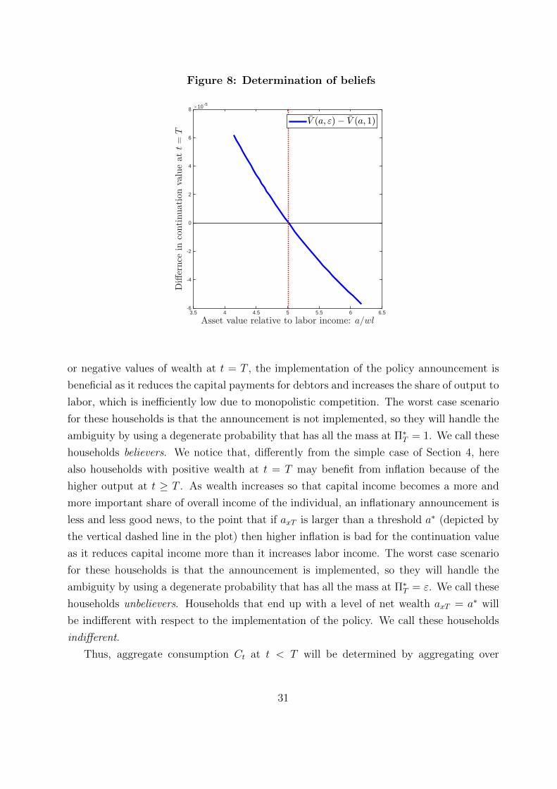
Figure 8: Determination of beliefs

Asset value relative to labor income: a=wl3.5 4 4.5 5 5.5 6 6.5

Di,

ernce

inco

ntinuation

valu

eatt=

T

#10 -5

-6

-4

-2

0

2

4

6

8

7V (a; ")! 7V (a; 1)

or negative values of wealth at t = T , the implementation of the policy announcement is

beneficial as it reduces the capital payments for debtors and increases the share of output to

labor, which is inefficiently low due to monopolistic competition. The worst case scenario

for these households is that the announcement is not implemented, so they will handle the

ambiguity by using a degenerate probability that has all the mass at Π∗T = 1. We call these

households believers. We notice that, differently from the simple case of Section 4, here

also households with positive wealth at t = T may benefit from inflation because of the

higher output at t ≥ T . As wealth increases so that capital income becomes a more and

more important share of overall income of the individual, an inflationary announcement is

less and less good news, to the point that if axT is larger than a threshold a∗ (depicted by

the vertical dashed line in the plot) then higher inflation is bad for the continuation value

as it reduces capital income more than it increases labor income. The worst case scenario

for these households is that the announcement is implemented, so they will handle the

ambiguity by using a degenerate probability that has all the mass at Π∗T = ε. We call these

households unbelievers. Households that end up with a level of net wealth axT = a∗ will

be indifferent with respect to the implementation of the policy. We call these households

indifferent.

Thus, aggregate consumption Ct at t < T will be determined by aggregating over

31

the demand of believers, unbelievers and indifferent households. As both believers and

unbelievers have degenerate beliefs about the equilibrium at t ≥ T , their demand at t < T

will be given by equations (32)-(33), where each type of household will have different

(degenerate) beliefs about the path of wt, rt and πt for t ≥ T . The demand of indifferent

households is instead given by the first order conditions in equation (12) together with the

inter-temporal budget constraint under the constraint that axT = a∗.

Numerical solution of the model We conjecture two paths of output Yt for t ≥ 0, one

for the case where the policy is implemented at t = T and one for the case where the policy

is not implemented at t = T . We notice that the two paths necessarily coincide at t < T .

We also notice that when Rt = R for t < T , Proposition 8 applies and the equilibrium

output in the case the policy is not implemented coincides with the steady state output.

Given the path of output, we can solve for the implied path of real wages, inflation and

interest rates from equations (6), (11) and (29). Given the path of prices ws, πs, rss≥0,

we can solve for the implied aggregate demand, Ct, using equation (32) for t ≥ T and the

solution to the household problem in equation (34) together with Ct =∫ 1

0ctx dx for t < T .

Finally, we obtain the implied value of output that satisfies the demand so obtained from

equation (31). We update our conjecture about Yt until convergence.

5.2 Calibration

The calibration exercise can be described as consisting of three different parts. The first part

deals with the choice of parameter values that govern household preferences and the firm

price adjustment technology. The second part deals with the calibration of the distribution

of households net financial assets. The third part deals with the calibration of the monetary

policy experiment.

Table 3 describes the choice of the parameters. We set the time period to be a quarter

and β = 0.985 so that the real interest rate is 6% in steady state (reference?).9 We set

σ = 2 so that the elasticity of interetempboral substitution (EIS) is 0.5, and ψ = 0.5 so that

the Frisch elasticity of labor supply is 2. They are both in the range of values commonly

used in the literature.10 The elasticity of substitution across different varieties is set to

θ = 3 to match a steady state labor share of output equal to 2/3. This value of θ is at the

lower end of the range of values typically used in macro models when estimating the price

9This choice of β implies that aggregate capital income is 12% as large as labor income in our model. Itis a conservative choice from the perspective of matching the capital income share of output. For instance,Elsby, Hobijn, and Sahin (2013) report estimates according to which the profit share is 20% of the payrollshare.

10See Guvenen (2006) for a review on the estimates of the EIS. See Keane and Rogerson (2012) for adiscussion of the Frisch elasticity.

32

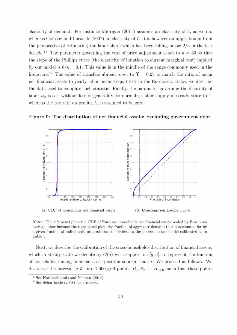
elasticity of demand. For instance Midrigan (2011) assumes an elasticity of 3, as we do,

whereas Golosov and Lucas Jr (2007) an elasticity of 7. It is however an upper bound from

the perspective of estimating the labor share which has been falling below 2/3 in the last

decade.11 The parameter governing the cost of price adjustment is set to κ = 30 so that

the slope of the Phillips curve (the elasticity of inflation to current marginal cost) implied

by our model is θ/κ = 0.1. This value is in the middle of the range commonly used in the

literature.12 The value of transfers abroad is set to Υ = 0.25 to match the ratio of mean

net financial assets to yearly labor income equal to 2 in the Euro area. Below we describe

the data used to compute such statistic. Finally, the parameter governing the disutility of

labor ψ0 is set, without loss of generality, to normalize labor supply in steady state to 1,

whereas the tax rate on profits, δ, is assumed to be zero.

Figure 9: The distribution of net financial assets: excluding government debt

Asset relative to labor income-50 0 50 100 150 200 250 300 350

Fra

ctio

n of

indi

vidu

als,

CD

F

0

0.1

0.2

0.3

0.4

0.5

0.6

0.7

0.8

0.9

1

(a) CDF of households net financial assets

Fraction of individuals0 0.1 0.2 0.3 0.4 0.5 0.6 0.7 0.8 0.9 1

Fra

ctio

n of

tota

l con

sum

ptio

n

0

0.1

0.2

0.3

0.4

0.5

0.6

0.7

0.8

0.9

1

(b) Consumption Lorenz Curve

Notes: The left panel plots the CDF of Euro are households net financial assets scaled by Euro areaaverage labor income; the right panel plots the fraction of aggregate demand that is accounted for bya given fraction of individuals, ordered from the richest to the poorest in our model calibrated as inTable 3.

Next, we describe the calibration of the cross-households distribution of financial assets,

which in steady state we denote by G(a) with support on [a, a], to represent the fraction

of households having financial asset position smaller than a. We proceed as follows. We

discretize the interval [a, a] into 1,000 grid points, B1, B2, . . . B1000, such that these points

11See Karabarbounis and Neiman (2014).12See Schorfheide (2008) for a review.

33

Table 3: Baseline Calibration

Model DataParameter Value Moment Value

β 0.985 Yearly real return 0.06

σ 2 Elasticity of intertemporal substitution 0.5

ψ 0.5 Frisch elasticity of labor supply 2

ψ0 0.66 Labor supply normalization 1

θ 3 Labor share 0.66

κ 30 Slope of the Phillips Curve 0.1

Υ 0.25 Mean net financial asset to yearly labor income 2

φ 1.5 Taylor rule response to inflation 1.5

ρr 0.8 Taylor rule inertia in nominal rate 0.8

T 6 Max fit to forward rates response at 2-10 years maturity -

ρ∗ 0.9 Max fit to forward rates response at 2-10 years maturity -

ε 1.0016 Max fit to forward rates response at 2-10 years maturity -

represent the permilles of the distribution, i.e. G(B1) = G(Bi+1) − G(Bi) = 0.001 for all

i < 1000. We then identify the grid points Bi, for i = 1, 2, ...1000 from the distribution of

net financial assets obtained from the Euro area Household Finance Consumption Survey

(HFCS). The data refers to 2010 except for Austria where the data refers to 2012. The

data cover all countries in the group of Euro 11 with the exclusion of Ireland, which is not

included in HFCS. Net Financial assets are calculated as the the difference between total

financial assets and total financial liabilities.13 In our benchmark calibration we do not in-

13Financial assets include Deposits (da2101); Mutual Funds (da2102); Bonds (da2103); non self-employment private business (da2104); value of self-employment business (da1140); shares of publiclytraded companies (ds2105); managed accounts (da2106 ); money owed to households (da2107); Other As-sets (da2108); Voluntary pensions plus whole life insurance (da2109). Financial liabilities is calculated asthe sum of outstanding balance of HMR mortgages (dl1110); outstanding balance of mortgages on other

34

clude government debt among the liabilities of the household. In an alternative calibration

we add government debt to the liabilities of the household.14 The left panel of Figure 9

plots the cumulated probability distribution of net financial assets, scaled by the average

yearly labor income of the Euro area, in the case where government debt is excluded by

household liabilities. The distribution displays substantial standard deviation and skew-

ness, about 23 and 116 respectively, and is characterized by a mean approximately equal

to 2. The distribution of net financial assets including government debt (not displayed)

is characterized by similar standard deviation and skewness, but lower mean which drops

to 0.35 of yearly labor income. The right panel of Figure 9 plots the Lorenz curve for the

distribution of consumption predicted by our model at the baseline calibration. It gives on

the vertical axis the fraction of total consumption accounted by the top x% of households

on the horizontal axis ordered by their financial wealth. As a result, the Lorenz curve is

always above the 45 degree line. The vertical dashed red line denotes the fraction of house-

holds that believe the inflationary announcement. These correspond to the top 10% of the

distribution of financial wealth and account for 20% of aggregate demand in our model.

Finally, we calibrate the monetary policy parameters. We set the parameters of the

interest rate rule in equation (6) to standard values, i.e. φ = 1.5 and ρr = 0.8. We choose

the horizon of the announcement T , its intensity ε, together with the persistence of the

inflation target ρ∗, to maximize the fit of the path of the nominal interest rate predicted by

our model with the path of nominal interest rates in the Euro area predicted at the time of

the announcement by Mario Draghi that started the Forwad Guidance Policy by the ECB

on July 4th 2013. In particular, we choose these parameters to match the difference in the

path of instantaneous forward rates associated to the yield curves of Triple A government

bonds in the Euro area between July 4th and July 2nd for maturities up to 10 years . We

plot such difference in the right panel of Figure 10 for maturities up to 10 years. In the

left panel of Figure 10 we plot instead the forward rates on July 2nd.15 We notice that

forward guidance announcement has had a substantial impact on the path of interest rates.

properties (dl1120 ); and outstanding balance of other non mortgage debt (dl1200). Statistics are weightedusing weights provided by HFCS (hw0010) and then aggregated by taking the simple mean of the valuesobtained using the five different implicates reported by HFCS (im0100).

14Government debt of the household is the product of the country specific level of net government debtper capita as reported in Table 1 of Adam and Zhu (2015) multiplied by the number of people in thehousehold who are older than 16 years of age as obtained by HFCS (dh0006).

15Effects are similar when focusing on the yield curve of the EOANIA Swap interest rate. The instanta-neous Forward rate is calculated using the methodology by Svensson (1995), “Estimating Forward InterestRates with the Extended Nelson and Siegel Method,” Sveriges Riksbank Quarterly Review 1995:3, pp13-26, as calculated by the ECB. We focus on government bonds rather than on the EONIA swap ratebecause the yield curve of government bonds is characterized also at maturity greater than 2 years, whilethe interest rate swap of the Eonia market is available only up to maturities of 2 years. The data areobtained at the datawarehouse of the ECB.

35

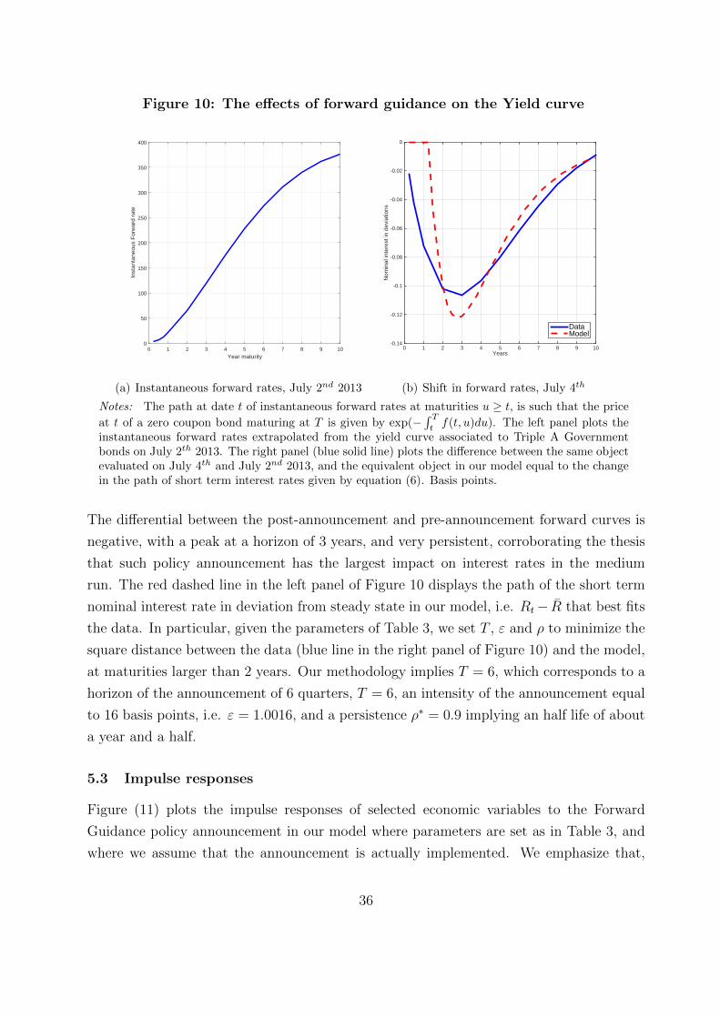
Figure 10: The effects of forward guidance on the Yield curve

0 1 2 3 4 5 6 7 8 9 10

Year maturity

0

50

100

150

200

250

300

350

400

Inst

anta

neou

s F

orw

ard

rate

(a) Instantaneous forward rates, July 2nd 2013

Years0 1 2 3 4 5 6 7 8 9 10

Nom

inal

inte

rest

in d

evia

tions

-0.14

-0.12

-0.1

-0.08

-0.06

-0.04

-0.02

0

DataModel

(b) Shift in forward rates, July 4th

Notes: The path at date t of instantaneous forward rates at maturities u ≥ t, is such that the price

at t of a zero coupon bond maturing at T is given by exp(−∫ T

tf(t, u)du). The left panel plots the

instantaneous forward rates extrapolated from the yield curve associated to Triple A Governmentbonds on July 2th 2013. The right panel (blue solid line) plots the difference between the same objectevaluated on July 4th and July 2nd 2013, and the equivalent object in our model equal to the changein the path of short term interest rates given by equation (6). Basis points.

The differential between the post-announcement and pre-announcement forward curves is

negative, with a peak at a horizon of 3 years, and very persistent, corroborating the thesis

that such policy announcement has the largest impact on interest rates in the medium

run. The red dashed line in the left panel of Figure 10 displays the path of the short term

nominal interest rate in deviation from steady state in our model, i.e. Rt− R that best fits

the data. In particular, given the parameters of Table 3, we set T , ε and ρ to minimize the

square distance between the data (blue line in the right panel of Figure 10) and the model,

at maturities larger than 2 years. Our methodology implies T = 6, which corresponds to a

horizon of the announcement of 6 quarters, T = 6, an intensity of the announcement equal

to 16 basis points, i.e. ε = 1.0016, and a persistence ρ∗ = 0.9 implying an half life of about

a year and a half.

5.3 Impulse responses

Figure (11) plots the impulse responses of selected economic variables to the Forward

Guidance policy announcement in our model where parameters are set as in Table 3, and

where we assume that the announcement is actually implemented. We emphasize that,

36

while the implementation of the monetary policy announcement will affect equilibrium

outcomes at t ≥ T , it has no effect on the equilibrium outcomes at t < T , as only beliefs

about the implementation matter for the equilibrium. The blue lines plot the responses

of our economy, the black dashed lines plot the responses that would be predicted in a

counterfactual economy where all households are assumed to believe the announcement.

The vertical red line denotes the time of the implementation of the announcement.

As a consequence of the application of Proposition 8, the economy behaves as a standard

representative agent new-keynesian economy after the implementation of the announcement

at t ≥ T , independently of the dynamics at t < T : output and inflation increase as

a consequence of the fall in nominal and real interest rates. Thus the monetary policy

is indeed expansionary once implemented. The economy behaves very differently from

the counterfactual (all believe) economy in the interim period between the announcement

and the implementation: output falls on impact of the announcement and keeps falling

until the implementation, whereas in the counterfatual economy the announcement would

have caused an output boom. The fall in output in our economy is driven by the fall

in demand of believers, who are households with larger financial asset position and are

hurt by the (eventual) implementation of the expansionary policy. Notice that also in the

counterfactual (all-believe) economy these households would reduce their demand. What

differentiates our economy from the counterfactual one is the behavior of households with

financial asset position low enough that they behave under the belief that the monetary

announcement will not be implemented at t = T . As these are the household that would

benefit the most from the fall in real rates, and would increase the most their demand if

they were to believe, their relative inaction matters substantially for the overall response

of aggregate demand. Intuitively, in the counterfactual (all believe) economy the higher

increase in demand of households with low financial asset positions exactly offsets the fall in

demand of households with high financial asset position, so that the distribution of wealth

is irrelevant. In our economy, the wealth distribution instead matters a lot.

We notice that household with low financial asset position (unbelievers) increase nev-

ertheless their demand at t < T . This is explained by the fall in the real interest rate that

takes place at t < T . Because of the substitution effect and the lower interest payment

on debt at t < T , these households will increase their consumption, but the increase in

consumption would have been much larger if these households were to believe that the real

rate will keep being low also at t ≥ T . As t approaches T , the positive impact on demand

of the substitution effect becomes smaller, so that household reduce their overall demand,

explaining the further fall in output. Finally, the fall in the real interest rate at t < T

is explained by the increase in inflation of forward-looking firms who we have assumed to

37

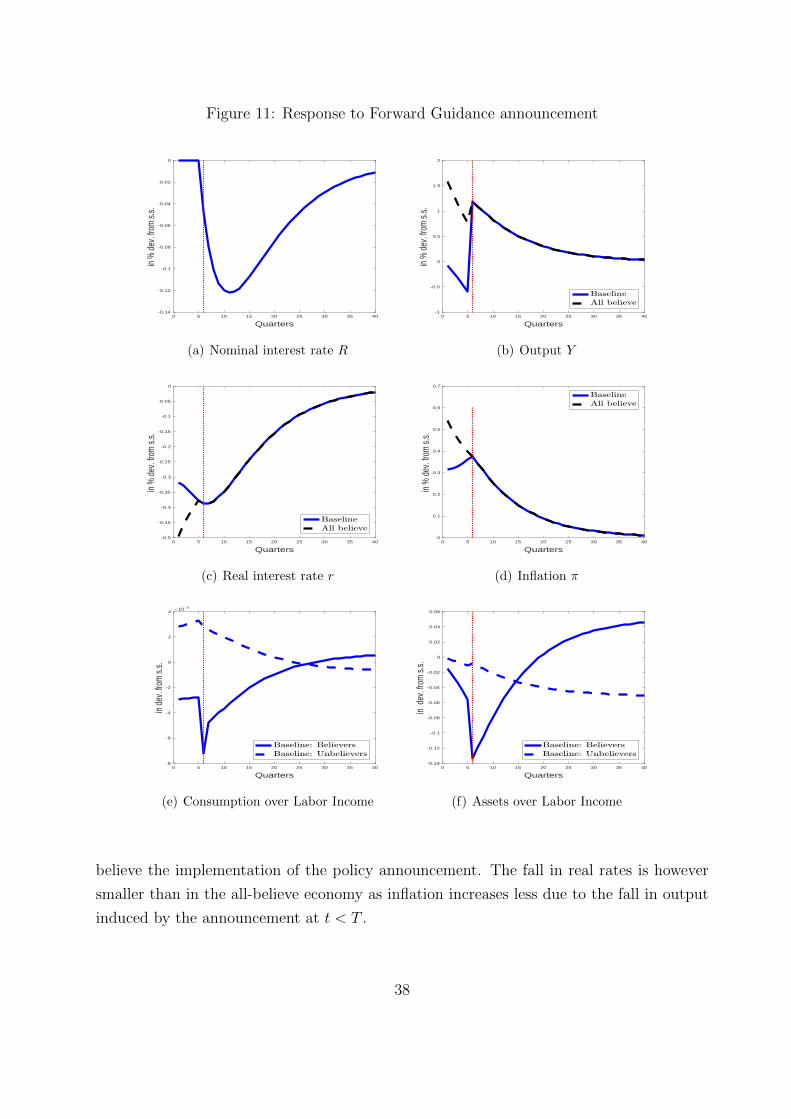
Figure 11: Response to Forward Guidance announcement

0 5 10 15 20 25 30 35 40

Quarters

-0.14

-0.12

-0.1

-0.08

-0.06

-0.04

-0.02

0

in %

dev

. fro

m s.

s.

(a) Nominal interest rate R

0 5 10 15 20 25 30 35 40

Quarters

-1

-0.5

0

0.5

1

1.5

2

in %

dev

. fro

m s.

s.

BaselineAll believe

(b) Output Y

0 5 10 15 20 25 30 35 40

Quarters

-0.5

-0.45

-0.4

-0.35

-0.3

-0.25

-0.2

-0.15

-0.1

-0.05

0

in %

dev

. fro

m s.

s.

BaselineAll believe

(c) Real interest rate r

0 5 10 15 20 25 30 35 40

Quarters

0

0.1

0.2

0.3

0.4

0.5

0.6

0.7

in %

dev

. fro

m s.

s.

BaselineAll believe

(d) Inflation π

0 5 10 15 20 25 30 35 40

Quarters

-8

-6

-4

-2

0

2

4

in de

v. fro

m s.

s.

#10 -3

Baseline: BelieversBaseline: Unbelievers

(e) Consumption over Labor Income

0 5 10 15 20 25 30 35 40

Quarters

-0.14

-0.12

-0.1

-0.08

-0.06

-0.04

-0.02

0

0.02

0.04

0.06

in d

ev. f

rom

s.s.

Baseline: BelieversBaseline: Unbelievers

(f) Assets over Labor Income

believe the implementation of the policy announcement. The fall in real rates is however

smaller than in the all-believe economy as inflation increases less due to the fall in output

induced by the announcement at t < T .

38

6 Robustness

In this section we perform a series of robustness exercises to assess the relevance of the as-

sumptions of our economic model. In each exercise, we change one assumption at the time.

When needed, we recalibrate the parameters governing the monetary policy experiment, T ,

ρ∗ and ε so that each economy we consider is consistent and observationally equivalent with

respect to the path of nominal interest rates described in Figure 10. The other parameters

are unchanged with respect to Table 3, unless a parameter is the object of the robustness

exercise.

Government debt into households liabilities. In this section we calibrate the distri-

bution of net financial assets including government debt, of which we plot the cumulative

distribution function in the left panel of Figure 12. As a result of the higher liabilities, the

mean value of net financial asset relative to labor income drops from 2 in the benchmark

case to 0.38 in this case. The right panel of Figure 12 plots the consumption Lorenz curve

in our model at new distribution of financial assets. Now, the fraction of individuals that

have enough financial assets drops from 10% in the benchmark case to 8% in this case,

accounting for 18% of aggregate consumption. The first row of Figure 13 plots the impulse

response of output (left panel) to the monetary policy announcement of a change in the

path of the inflation target (right panel), that is then actually implemented, in the base-

line model (blue solid line) and in the counterfactual with government debt (black dashed

line). As a result of the different parametrization of the distribution of financial assets,

the estimated path of the inflation target is different from the baseline, displaying a larger

drop at the time of implementation, T = 6. This explains the larger response of output at

T = 6. In the interim period, t < T , the output response with government debt is larger

than in the baseline model, but the economy nevertheless experiences a recession a year

after the announcement. Moreover, the cumulated output gain in the five quarters after the

announcement is 0.6%, much smaller than the 5.8% output gain in the counterfactual all

believe economy displayed in Figure 11. Thus we conclude that, even if households were to

incorporate government debt as part of their liabilities, the Forward Guidance announce-

ment would have been far less effective in our model than in the standard homogeneous

beliefs economy.

Firms do not believe the announcement. In this section we assume that firms don’t

believe that the announcement will be implemented and assign a probability zero to this

happening. We notice that this assumption does not affect the path of the nominal interest

rates which are constant by assumption at t < T and independent of past beliefs at t ≥ T .

39

Figure 12: The distribution of net financial assets: including government debt

Asset relative to labor income-50 0 50 100 150 200 250 300 350

Fra

ctio

n of

indi

vidu

als,

CD

F

0

0.1

0.2

0.3

0.4

0.5

0.6

0.7

0.8

0.9

1

(a) CDF of households NFA

Fraction of individuals0 0.1 0.2 0.3 0.4 0.5 0.6 0.7 0.8 0.9 1

Fra

ctio

n of

tota

l con

sum

ptio

n

0

0.1

0.2

0.3

0.4

0.5

0.6

0.7

0.8

0.9

1

(b) Consumption Lorenz Curve

Notes: The left panel plots the CDF of Euro are households net financial assets scaled by Euro areaaverage labor income, net of government debt; the right panel plots the fraction of aggregate demandthat is accounted for by a given fraction of individuals, ordered from the richest to the poorest themodel.

The output response is identical to our baseline case at ≥ T , but differs from it before at

t < T . In particular, the output drops more at the time of the announcement and then is

almost invariant until the implementation. The reason is that firms are not front-loading

the future inflation in the current prices as they don’t believe the announcement and, as a

result, the real rate is almost constant in the interim period, so that the drop in output is

all driven by the fall in demand of wealthier households.

Taylor rule at t < T . In this section we assume that the nominal interest rate is not

constant at t < T but is instead given by equation (6) at all t. We reestimate the path of

the inflation target, displayed in the third row of Figure 13, and plot the output response

in the left panel. We notice that the output drops on impact of the announcement, and

then changes little until the time of the implementation relatively to the dynamics of the

output in the baseline economy. This is due to the reaction of the nominal interest rate

to inflation in the interim period that reduces the dynamics of the real rate, which instead

falls much more when the nominal rate is constant as in the baseline model, and inflation

rises.

Announcement of monetary policy tightening. In this section we study the output

effect of an announcement of a deflationary in our baseline economy. All parameter are

as in Table 3, but for the inflation target at t = T which we instead assume equal to ε =

40

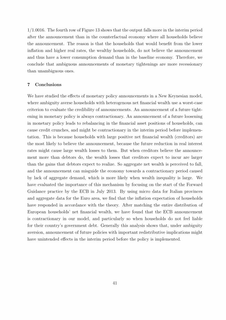
1/1.0016. The fourth row of Figure 13 shows that the output falls more in the interim period

after the announcement than in the counterfactual economy where all households believe

the announcement. The reason is that the households that would benefit from the lower

inflation and higher real rates, the wealthy households, do not believe the announcement

and thus have a lower consumption demand than in the baseline economy. Therefore, we

conclude that ambiguous announcements of monetary tightenings are more recessionary

than unambiguous ones.

7 Conclusions

We have studied the effects of monetary policy announcements in a New Keynesian model,

where ambiguity averse households with heterogenous net financial wealth use a worst-case

criterion to evaluate the credibility of announcements. An announcement of a future tight-

ening in monetary policy is always contractionary. An announcement of a future loosening

in monetary policy leads to rebalancing in the financial asset positions of households, can

cause credit crunches, and might be contractionary in the interim period before implemen-

tation. This is because households with large positive net financial wealth (creditors) are

the most likely to believe the announcement, because the future reduction in real interest

rates might cause large wealth losses to them. But when creditors believe the announce-

ment more than debtors do, the wealth losses that creditors expect to incur are larger

than the gains that debtors expect to realize. So aggregate net wealth is perceived to fall,

and the announcement can misguide the economy towards a contractionary period caused

by lack of aggregate demand, which is more likely when wealth inequality is large. We

have evaluated the importance of this mechanism by focusing on the start of the Forward

Guidance practice by the ECB in July 2013. By using micro data for Italian provinces

and aggregate data for the Euro area, we find that the inflation expectation of households

have responded in accordance with the theory. After matching the entire distribution of

European households’ net financial wealth, we have found that the ECB announcement

is contractionary in our model, and particularly so when households do not feel liable

for their country’s government debt. Generally this analysis shows that, under ambiguity

aversion, announcement of future policies with important redistributive implications might

have unintended effects in the interim period before the policy is implemented.

41

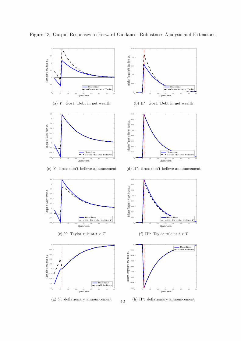
Figure 13: Output Responses to Forward Guidance: Robustness Analysis and Extensions

0 5 10 15 20 25 30 35 40

Quarters

-1

-0.5

0

0.5

1

1.5

2Ou

tput in

% de

v. fro

m s.s

.

BaselineGovernment Debt

(a) Y : Govt. Debt in net wealth

0 5 10 15 20 25 30 35 40

Quarters

0

0.05

0.1

0.15

0.2

0.25

Inflat

ion T

arge

t in %

dev.

from

s.s.

BaselineGovernment Debt

(b) Π∗: Govt. Debt in net wealth

0 5 10 15 20 25 30 35 40

Quarters

-0.6

-0.4

-0.2

0

0.2

0.4

0.6

0.8

1

1.2

Outpu

t in %

dev.

from

s.s.

BaselineFirms do not believe

(c) Y : firms don’t believe annoucement

0 5 10 15 20 25 30 35 40

Quarters

0

0.02

0.04

0.06

0.08

0.1

0.12

0.14

0.16

Inflat

ion T

arge

t in %

dev.

from

s.s.

BaselineFirms do not believe

(d) Π∗: firms don’t believe announcement

0 5 10 15 20 25 30 35 40

Quarters

-0.6

-0.4

-0.2

0

0.2

0.4

0.6

0.8

1

1.2

Outpu

t in %

dev.

from

s.s.

BaselineTaylor rule before T

(e) Y : Taylor rule at t < T

0 5 10 15 20 25 30 35 40

Quarters

0

0.02

0.04

0.06

0.08

0.1

0.12

0.14

0.16

Inflat

ion T

arge

t in %

dev.

from

s.s.

BaselineTaylor rule before T

(f) Π∗: Taylor rule at t < T

0 5 10 15 20 25 30 35 40

Quarters

-1.8

-1.6

-1.4

-1.2

-1

-0.8

-0.6

-0.4

-0.2

0

Outpu

t in %

dev.

from

s.s.

BaselineAll believe

(g) Y : deflationary announcement

0 5 10 15 20 25 30 35 40

Quarters

-0.16

-0.14

-0.12

-0.1

-0.08

-0.06

-0.04

-0.02

0

Inflat

ion T

arge

t in %

dev.

from

s.s.

BaselineAll believe

(h) Π∗: deflationary announcement42

References

Adam, K. and J. Zhu (2015). Price level changes and the redistribution of nominal wealth

across the Euro Area. Journal of the European Economic Association.

Andrade, P., G. Gaballo, E. Mengus, and B. Mojon (2015). Forward Guidance and

heterogeneous beliefs. Available at SSRN 2677644 .

Auclert, A. (2015). Monetary policy and the redistribution channel. Mimeo Princeton.

Backus, D., A. Ferriere, and S. Zin (2015, January). Risk and ambiguity in models of

business cycles. Journal of Monetary Economics 69, 42–63.

Caballero, R. J. and E. Farhi (2014). The safety trap. Technical report, National Bureau

of Economic Research.

Coeure, B. (2013). The usefulness of Forward Guidance.

https://www.ecb.europa.eu/press/key/date/2013/, Speech before the Money

Marketeers Club of New York, 26 September 2013.

Coibion, O., Y. Gorodnichenko, and S. Kumar (2015). How do firms form their expec-

tations? New survey evidence. American Economic Review .

Dimmock, S. G., R. Kouwenberg, O. S. Mitchell, and K. Peijnenburg (2016). Ambigu-

ity aversion and household portfolio choice puzzles: Empirical evidence. Journal of

Financial Economics 119 (3), 559–577.

Doepke, M. and M. Schneider (2006). Inflation and the redistribution of nominal wealth.

Journal of Political Economy 114 (6), 1069–1097.

Doepke, M., M. Schneider, and V. Selezneva (2015). Distributional effects of monetary

policy. Working Papers 14, Hutchins Center at Brookings.

Eggertsson, G. B. and M. Woodford (2003). Zero bound on interest rates and optimal

monetary policy. Brookings Papers on Economic Activity 2003 (1), 139–233.

Elsby, M. W., B. Hobijn, and A. Sahin (2013). The decline of the US labor share.

Brookings Papers on Economic Activity 2013 (2), 1–63.

Epstein, L. G. and M. Schneider (2003). Recursive multiple-priors. Journal of Economic

Theory 113 (1), 1–31.

Fisher, I. (1933). The debt-deflation theory of great depressions. Econometrica 1 (4),

337–357.

Gilboa, I. and D. Schmeidler (1989). Maxmin expected utility with non-unique prior.

Journal of Mathematical Economics 18 (2), 141–153.

43

Golosov, M. and R. E. Lucas Jr (2007). Menu costs and Phillips curves. Journal of

Political Economy 115 (2).

Greenwood, J., Z. Hercowitz, and G. W. Huffman (1988). Investment, capacity utiliza-

tion, and the real business cycle. American Economic Review 78 (3), 402–17.

Guvenen, F. (2006). Reconciling conflicting evidence on the elasticity of intertemporal

substitution: A macroeconomic perspective. Journal of Monetary Economics 53 (7),

1451–1472.

Ilut, C., P. Krivenko, and M. Schneider (2015). Uncertainty aversion and heterogeneous

beliefs in linear models. Mimeo Duke University .

Ilut, C. and M. Schneider (2014). Ambiguous business cycles. American Economic Re-

view 104 (2), 2368–2399.

Ilut, C., R. Valchev, and N. Vincent (2016). Paralyzed by fear: Rigid and discrete pricing

under demand uncertainty. Mimeo Duke University .

Kaplan, G., B. Moll, and G. Violante (2016a). Monetary policy according to HANK.

NBER Working Paper 21897.

Kaplan, G., B. Moll, and G. Violante (2016b). A note on unconventional monetary policy

in HANK. Mimeo, New York University and Princeton University.

Karabarbounis, L. and B. Neiman (2014). The global decline of the labor share. Quarterly

Journal of Economics 129 (1).

Keane, M. and R. Rogerson (2012). Micro and macro labor supply elasticities: A re-

assessment of conventional wisdom. Journal of Economic Literature 50 (2), 464–476.

Lane, P. R. and G. M. Milesi-Ferretti (2007). The External Wealth of Nations Mark II:

Revised and extended estimates of foreign assets and liabilities, 1970-2004. Journal

of International Economics 73 (2), 223–250.

McKay, A., E. Nakamura, and J. Steinsson (2015). The power of Forward Guidance

revisited. Mimeo, Columbia University.

Midrigan, V. (2011). Menu costs, multiproduct firms, and aggregate fluctuations. Econo-

metrica 79 (4), 1139–1180.

Rotemberg, J. (1982). Sticky prices in the United States. Journal of Political Econ-

omy 90, 1187–1211.

Schorfheide, F. (2008). DSGE model-based estimation of the New Keynesian Phillips

curve. FRB Richmond Economic Quarterly 94 (4), 397–433.

44

Svensson, L. (1995). Estimating forward interest rates with the extended Nelson and

Siegel method. Sveriges Riksbank Quarterly Review 3, 13–26.

Swanson, E. T. (2016). Measuring the effects of federal reserve forward guidance and asset

purchases on financial markets. Technical report, University of California, Irvine.

Del Negro, M., M. P. Giannoni, and C. Patterson (2015). The Forward Guidance puzzle.

Mimeo, New York Fed.

ECB (2014). The ECB’s Forward Guidance. Monthly Bulletin April, 65–73.

Tobin, J. (1982). Asset Accumulation and Economic Activity: Reflections on Contempo-

rary Macroeconomic Theory. University Of Chicago Press.

Wiederholt, M. (2014). Empirical properties of inflation expectations and the Zero Lower

Bound. Goethe University Frankfurt .

45

A Data appendix

We describe the source of data for (i) realized and expected inflation in the Euro Area, (ii)Italian provinces, and (iii) the Net Financial Assets of European households.

A.1 Euro Area Data on realized and expected inflation

We focus on the group of Euro 11 countries: Austria, Belgium, Finland, France, Germany,Ireland, Italy, Luxembourg, Portugal, Spain, and Netherlands.

Core Inflation is equal to the yearly log differences in the Harmonised Index of ConsumerPrices (HICP) energy and unprocessed food multiplied by 100, which comes from theEurostat data warehouse available at “http://ec.europa.eu/eurostat/”.

Price expectations data come from the Joint Harmonized Programme of Business and Con-sumer Surveys run by the European Commission. These surveys are administered at amonthly frequency. The key advantage of the Consumer Survey is that it directly asksEuropean households for their expectations about future inflation, which makes the sur-vey very different from the commonly used Survey of Professional Forecasters, which justfocuses on professionals. The sample size for each survey varies across countries. Priceexpectations are obtained from the following question: “By comparison with the past 12months, how do you expect that consumer prices will develop in the next 12 months? Theywill (i) increase more rapidly; (ii) increase at the same rate; (iii) increase at a slower rate;(iv) stay about the same; (v) fall. Probabilities are calculated in terms of balances (differ-ences between people saying that the answer is very likely versus people saying the answer itis unlikely) so that Price expectations are calculated as equal to (fi+1/2fii−1/2fiv−fv)×10,where fj = i, ii, iii, iv, v is the fraction of individuals who opted for option j in the survey.The series are seasonally adjusted by the Commission.

Creditor vs debtor countries Creditor countries are Austria, Finland, Germany, Luxembourg,and Netherlands. Others countries include all the remaining countries in the group of Euro11 countries. Countries are classified using their Net Foreign Asset Position as obtainedfrom the External Wealth of Nation Mark II (EWN), see Lane and Milesi-Ferretti (2007).The only exception is Austria that according to the last observation in the EWN dataset,which pertains to 2011, had a Net Foreign Asset position over GDP ratio of -4.5%. SinceAustria has accumulated large current account surpluses which average 2 percent of GDPin all the following years since 2011, we include it in the group of creditor countries. Resultsare robust to whether Austria is treated as a creditor or a debtor country.

A.2 Italian data

Our Italian data come from the Italian statistical institute (ISTAT), from the Survey ofInflation Expectations ran by the Bank of Italy and Sole24Ore (which is the main Italiannational daily business newspaper), and from the Survey of Households Income and Wealth,administered by the Bank of Italy.

Realized inflation at the province level is obtained directly from ISTAT, as extracted fromthe I.Stat online archive. We focus on the general price index, denoted as pgen in the

46

ISTAT database. Realized inflation in the province corresponds to the yearly log-differenceof the general price index in the province. We take yearly log-differences, because the ECBmonitors price stability on the basis of the annual rate of change of the Harmonised Indexof Consumer Prices (HICP) and because of the phrasing of the inflation expectations data,see below.

Expected inflation measures 2-quarters-ahead expected inflation, by averaging the reportedestimates of all observations in the province in the Survey of Inflation Expectations ran bythe Bank of Italy and Sole24Ore. The disaggregated province level data are confidentialdata kindly made available to us by the Bank of the Italy. The Survey of Inflation Ex-pectations is ran at a quarterly frequency since 1999. Data is gathered in March, June,September and December. The sample comprises about 800 companies, operating in allindustries including construction. Entrepreneurs in the company are asked to predict theConsumer price inflation in Italy 6 months ahead, by answering the following question:“[If the survey is ran in June 2013] What do you think consumer price inflation in Italy,measured by the 12-month change in the Harmonized Index of Consumer Prices (HICP),will be in December 2013?”. Notice that entrepreneurs are asked to predict the evolutionof the same index (HICP at the national level) . In practice, here we are assuming that thereplies of entrepreneurs in a province reflect the average beliefs of all agents in the province.

Net Financial Assets (NFA) Our data on the NFA of Italian households come from the Surveyof Household Income and Wealth (SHIW), which is administered by the Bank of Italy to arepresentative sample of Italian households. The survey, which is currently ran at a biannualfrequency, collects detailed data on households’ balance sheets. Each wave surveys about8,000 households, which, after using the weights provided by SHIW (mnemonic Pesofitin SHIW), are fully representative of the Italian resident population. To increase samplesize, we rely on both the 2010 and the 2012 waves of SHIW. NFA are calculated as thedifference between the sum of households’ holdings of postal deposits, saving certificatesand CDs (mnemonic shiwaf1 in SHIW), government securities (mnemonic shiwaf2 in SHIW)and other securities (mnemonic shiwaf3 in SHIW) minus the sum of households financialliabilities to banks and other financial companies (mnemonic shiwpf1 in SHIW) plus tradedebt (mnemonic shiwpf2 in SHIW) plus liabilities to other households (mnemonic shiwpf3in SHIW).

Creditor household is a household with positive NFA, see the construction of the variableNFA for details.

Fraction of creditor households For each province we calculate the pre-announcement fractionof creditor households, by using the 2010 and the 2012 waves of SHIW. To calculate thefraction, we weight each household according to the weights provided by SHIW (mnemonicPesofit).

Inflation expectation bias In each province i and quarter t, we calculate the difference betweenexpected inflation, and future realized inflation, which corresponds to equation (1) in the maintext.

47

A.3 European households’ Net Financial Assets in HFCS

The Eurosystem Household Finance and Consumption Survey (HFCS) collects fully har-monised information on the asset portfolio allocation of households and their consumptionexpenditures in all euro area 11 countries (other than Ireland). Wealthy individuals areover-sampled to characterize well the right tail of the income and wealth distribution ofEuropean households. Within each country, the sum of the estimation weights equalsthe total number of households in the country, so that the sum of weights in the wholedataset equals the total number of households in the 10 countries of Euro 11 we consider.The structure of HFCS resembles that of the Survey of Consumer Finances in the US. Toaccount for measurement error and missing observations, HFCS reports five separate im-putation replicates (implicates) for each record. All statistics are calculated following theprocedure suggested by HFCS: for each implicate we calculate the desired statistic usingHFCS weights (mnemonic hw0010) and then average across the five implicates (mnemonicim0100). The surveys in each country were carried out in 2010 except in Finland andNetherlands where it was carried out in 2009 and in Spain where it was carried out in 2008.All statistics are deflated at 2010 prices.

Net Financial Assets (NFA) are calculated as the the difference between total financial assetsand total financial liabilities. Financial assets include (i) deposits (mnemonic da2101); (ii)mutual funds (mnemonic da2102); (iii) bonds (mnemonic da2103); (iv) non self-employmentprivate business (mnemonic da2104); (v) value of self-employment business (mnemonicda1140); (vi) shares of publicly traded companies (mnemonic ds2105); (vii) managed ac-counts (mnemonic da2106 ); (viii) money owed to households (mnemonic da2107); (ix) otherassets (mnemonic da2108); and (x) voluntary pensions plus whole life insurance (mnemonicda2109). Financial liabilities are the sum of (i) outstanding balance of mortgages on house-hold main residence (mnemonic dl1110); (ii) outstanding balance of mortgages on otherproperties (mnemonic dl1120 ); and (iii) outstanding balance of other non mortgage debt(mnemonic dl1200).

Net Financial Assets (NFA) including government debt is obtained by subtracting to NFA, theper household government debt of the country where the household resides. The household’scountry of residence is obtained from mnemonic sa0100. Per household government debt isthe product of the country specific level of net government debt per capita as reported inTable 1 of Adam and Zhu (2015) multiplied by the country’s average number of people inthe household who are older than 16 years of age as obtained by HFCS (mnemonic dh0006).

Consumption expenditures are the sum of the consumption expenditures during the last 12months on food and beverages at home (mnemonic hi0100) and on food and beveragesoutside home (mnemonic hi0200).

Average labor income in the Euro Area is calculated by averaging the employee income ofall household members (mnemonic di1100) for all households whose household head hasbetween 20 and 65 years of age. The mnemonic for the age of the household head is ra0300.The resulting average labor income is 21631 Euros.

48

B Proofs

Proof of Proposition ?? We start by proving point 2). At t ≥ T uncertainty aboutthe path of nominal interest rates and inflation is resolved. From the first order conditionto the household problem in equation (12) and its budget constraint in (5) we obtain theoptimal path of consumption:

cxt+j = ψ0

l1+ψt+j

1 + ψ+

j∏s=1

(β rt+s)1σ

(cxt − ψ0

l1+ψxt

1 + ψ

),

cxt +∞∑j=1

j∏s=1

r−1t+s cxt+j = axt rt + wtlxt + st +

∞∑j=1

j∏s=1

r−1t+s (wt+jlt+j + st+j) .

Combining the two expressions and using ψ0 l1+ψxt = wtlxt we have:

cxt +

(cxt −

wtlxt1 + ψ

)αxt = axt rt + wtlxt + st +

∞∑j=1

(j∏s=1

r−1t+s

)ψ

1 + ψ(wt+jlt+j + st+j) ,

implying equation(33). The path of real assets is given by

axt+1 = axt rt + wt lxt + st − cxt . (35)

We next prove point 1). We notice that from the equilibrium conditions in the financialmarkets in (27) we have

∫axt rtdx =

∫axt+1dx + Dt − Υ. By iterating forward we have∫

axt rtdx =∑∞

j=0 qt,t+j (Dt −Υ). Using this result into equation (33) we obtain equation(32).

Proof of Proposition 7 Using ρ = 0 and τ = 1 in the AD and AS equations andassuming Π∗1 = ε we have

aj1 − aj0 =ε−

1σ N0 − N + aj0(R− 1)(ε−

1σ − ε−1)

(R− 1) ε−1 + ε−1σ

, (36)

aj2 − aj0 =ε−

1σ N0 − N + aj0(R− 1)

(ε−

1σR−εR−1− 1)

R− 1 + ε1− 1σ

, (37)

where j = c, d rand recall that ac2 = B′ε−1, ac1 = B′, ac0 = B, ad2 = −B′ε−1, ad1 = −B′and ad0 = −B. Using equation (14) we have N0 = N ε

1σ , which together with the last

equations implies ac1−ac0 > 0 and ac2−ac0 < 0 if ε > 1, and ac1−ac0 > 0 and ac2−ac0 > 0if ε < 1.Rebalancing with ambiguity: ε > 1. Using ρ = 1 and ε > 1 in the AD and AS equations,

49

we have that ac1−ac0 and ac2−ac0 are given by equations (36) and (37) respectively, while

ad1 − ad0 =N0 − NR

, and ad2 − ad0 = ε−1N0 − NR

+ (ε−1 − 1) ad0

When ε > 1 and ρ = 1, using equation (14) we have:

N0 = N (ω ε1σ + 1− ω)−B κ (1− ε

1σ−1) < N ε

1σ

Using the last equation and the definitions of ω and κ we have:

ad2 − ad0 = ε−1 N

Rω (ε

1σ − 1)− ad0

[1 − 2ε−1 R

R− 1 + (R + 1) ε1− 1σ

]> 0 .

Moreover, comparing equation (37) at j = c in the case with ambiguity to the case when allbelieve we have that ac2 − ac0 is smaller (and ad2 − ad0 is smaller) in the case of ambiguitythan when all believe because equilibrium output N0 is smaller.

Rebalancing with ambiguity: ε < 1.Using ρ = −1 and ε < 1 in the AD and AS equations, we have that ad1 − ad0 and

ad2 − ad0 are given by equations (36) and (37) respectively, while

ac1 − ac0 =N0 − NR

, and ac2 − ac0 = ε−1N0 − NR

+ (ε−1 − 1) ac0

When ε < 1 and ρ = −1, using equation (14) we have:

N0 = N (ω + (1− ω) ε1σ )−B κ (ε

1σ−1 − 1) < N ε

1σ

Using the last equation and the definitions of ω and κ we have:

ac2 − ac0 =κ

R− 1

[ε−1N (ε

1σ − 1)−B

((R− 1) ε

1σ−1 + R (−2ε−1 + 1) + 1

)],

implying ac2 − ac0 < 0 if and only if

B <N ε−1 (1− ε 1

σ )

R (2ε−1 − 1− ε 1σ−1) + ε

1σ−1 − 1

.

Moreover, comparing equation (37) at j = d in the case with ambiguity to the case whenall believe we have that ad2−ad0 is smaller (and ac2−ac0 is larger) in the case of ambiguitythan when all believe because equilibrium output N0 is smaller.

50

Derivations:

R(ad2 − ad0) = ε−1N ω (ε1σ − 1)− ε−1 ad0 κ (ε

1σ−1 − 1) + R ad0 (ε−1 − 1)

= −ε−1N ω (1− ε1σ )− ad0κ

[ε−1 (ε

1σ−1 − 1) +

2

R− 1(1− ε−1) + (ε

1σ−1 + 1)(1− ε−1)

]= −ε−1N ω (1− ε

1σ )− R ad0

R + 1 + (R− 1) ε1σ−1

[(R− 1) (−2ε−1 + 1 + ε

1σ−1) + 2 (1− ε−1)

]= −ε−1N ω (1− ε

1σ )− R ad0ε

1− 1σ

R− 1 + (R + 1) ε1− 1σ

[(R− 1) ε

1σ−1 − R (2ε−1 − 1) + 1

]= −ε−1N ω (1− ε

1σ )− R ad0

[1− 2ε−1 R

R− 1 + (R + 1) ε1− 1σ

]

R(ac2 − ac0) = ε−1N (1− ω) (ε1σ − 1)− ε−1 ac0 κ (ε

1σ−1 − 1) + R ac0 (ε−1 − 1)

=κ ε−1N (ε

1σ − 1)

R− 1−B κ

[ε−1 (ε

1σ−1 − 1) +

2

R− 1(1− ε−1) + (ε

1σ−1 + 1)(1− ε−1)

]=κ ε−1N (ε

1σ − 1)

R− 1− B κ

R− 1

[(R− 1) (−2ε−1 + 1 + ε

1σ−1) + 2 (1− ε−1)

]=

κ

R− 1

[ε−1N (ε

1σ − 1)−B

((R− 1) ε

1σ−1 + R (−2ε−1 + 1) + 1

)]so that ac2 − ac0 < 0 if and only if

B <N ε−1 (1− ε 1

σ )

R (2ε−1 − 1− ε 1σ−1) + ε

1σ−1 − 1

C Extensions of the simple model of Section 4

C.1 Long term nominal bonds

In this section we extend our model to allow for long term nominal bonds and show thatthe equilibrium of the economy is unaffected. In particular, we assume that households cannow trade two different assets a one period real bond as before (whose units are denotedby ax), that for each unit bought in period t pays rt+1 units at t+ 1, and a perpetual bond(whose units are denoted by zx) that pays a constant nominal return i each period, andhas a price µt in period t. Let Bt = act + µt zct be the value of financial assets held bycreditor households, so that −Bt = adt + µt zdt is the value owed by debtors. Assume, asbefore, that creditors are half of the population. Equilibrium in the financial market nowrequires zct + zdt = 0 and act + adt = 0.

For given beliefs, the first order conditions of the household x problem with respect to

51

axt+1 and zxt+1 are given by equation (12) and by

µt

(cxt − ψ0

l1+ψxt

1 + ψ

)−σ= β Ext

[(cxt+1 − ψ0

l1+ψxt+1

1 + ψ

)−σµt+1 + i

Πt+1

].

We now conjecture and verify that the equilibrium obtained in this economy with long-term nominal bonds is identical to the one obtained in Section 4, when only short termbonds are present. The proof is immediate once we show that the long-term nominalbond and the short term real assets are equivalent in our model, so that the household isindifferent between holding one or the other, and the portfolio choice is irrelevant. Underthe conjecture that the equilibrium is invariant, we have that Rt = R for all t, implying rt =R/Πt for all t. Moreover, under the conjectured equilibrium households have degenerate

beliefs so that the first order conditions to the household problem imply: µt+1+iµt

= R, sothat the evolution of the price of the nominal bond has to be such that the nominal returnper period is R. Therefore, the short term real bond and the long-term nominal bond areequivalent as their return only varies as a result of variation in the realization of inflation.

D Solution of the quantitative model

We set a date T large arbitrarily large at which the economy is back to steady state whereΠt = 1, Yt = Y and the real wage wt = ψ0Y

ψ for all t > T . We recall that δ = 0 so thatthere are no subsidies to the household. We then conjecture a path of real wages, wtTt=0.Given the path of real wages, we use the equilibrium condition in the labor market to obtain

the path of labor supply and output, Yt = lxt = (wt/ψ0)1ψ . Given the path of output and

real wages, we use the sequence of equations (29) for each t and equations (6) to jointlydetermine the path of inflation Πt, of nominal interest rates Rt and therefore of real rates,rt = Rt/Πt − 1. Given the path of inflation and the equilibrium condition in the goodsmarket we obtain aggregate consumption as cxt = Yt

(1− κ

2(Πt − 1)2) − φ. Furthermore,

from equation (6) we obtain the path of nominal interest rates Rt and therefore real rates,rt = Rt/Πt − 1. Given the dynamics of aggregate variables we are ready to solve forthe household problem. We do this in two steps. We first solve the household problemafter the implementation of the announcement, i.e. for t ≥ T , and conditional on a givenimplementation of the announcement; in the second step we obtain household consumptionand saving decisions for t < T for given beliefs of the household about the implementationof the announcement at t = T .

The solution to the household problem at t ≥ T is given by Proposition ??. In thecase of the announcement not being implemented we have w1

t = ψ0 Yψ for t ≥ T . In the

case of the announcement being implemented instead, we update the guess for w0t Tt=T

until Yt = (cxt + Υ)/(1− κ

2π2t

)is satisfied. Once we have determined the equilibrium path

of wmt ∞t=T , and associated equilibrium aggregate variables, we are able to determine thevalue function of an household j with real asset value axt at the beginning of period T ,as a function of the implementation of the monetary announcement, denoted by V m

T (axt).

Such value function is given by∑∞

j=0 βj

(cxt+j − ψ0

l1+ψt+j

1+ψ

)1−σ

/1− σ, where cxt+j and lt+j

52

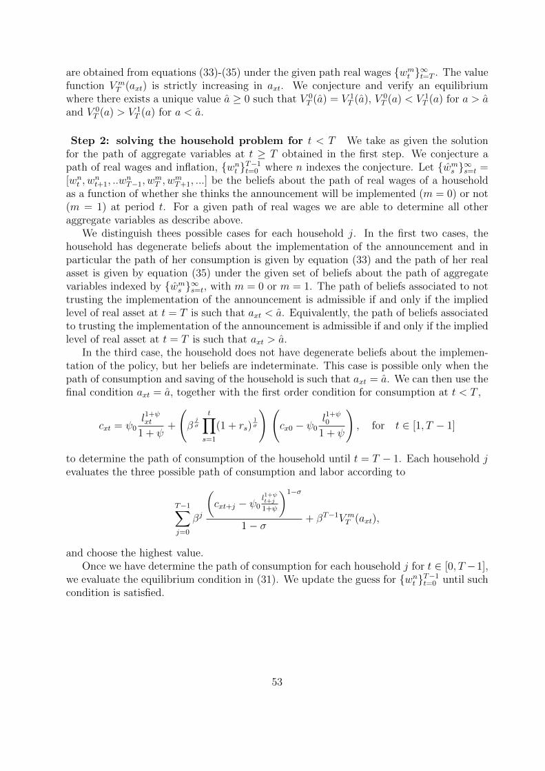
are obtained from equations (33)-(35) under the given path real wages wmt ∞t=T . The valuefunction V m

T (axt) is strictly increasing in axt. We conjecture and verify an equilibriumwhere there exists a unique value a ≥ 0 such that V 0

T (a) = V 1T (a), V 0

T (a) < V 1T (a) for a > a

and V 0T (a) > V 1

T (a) for a < a.

Step 2: solving the household problem for t < T We take as given the solutionfor the path of aggregate variables at t ≥ T obtained in the first step. We conjecture apath of real wages and inflation, wnt T−1

t=0 where n indexes the conjecture. Let wms ∞s=t =[wnt , w

nt+1, ..w

nT−1, w

mT , w

mT+1, ...] be the beliefs about the path of real wages of a household

as a function of whether she thinks the announcement will be implemented (m = 0) or not(m = 1) at period t. For a given path of real wages we are able to determine all otheraggregate variables as describe above.

We distinguish thees possible cases for each household j. In the first two cases, thehousehold has degenerate beliefs about the implementation of the announcement and inparticular the path of her consumption is given by equation (33) and the path of her realasset is given by equation (35) under the given set of beliefs about the path of aggregatevariables indexed by wms ∞s=t, with m = 0 or m = 1. The path of beliefs associated to nottrusting the implementation of the announcement is admissible if and only if the impliedlevel of real asset at t = T is such that axt < a. Equivalently, the path of beliefs associatedto trusting the implementation of the announcement is admissible if and only if the impliedlevel of real asset at t = T is such that axt > a.

In the third case, the household does not have degenerate beliefs about the implemen-tation of the policy, but her beliefs are indeterminate. This case is possible only when thepath of consumption and saving of the household is such that axt = a. We can then use thefinal condition axt = a, together with the first order condition for consumption at t < T ,

cxt = ψ0l1+ψxt

1 + ψ+

(βjσ

t∏s=1

(1 + rs)1σ

) (cx0 − ψ0

l1+ψ0

1 + ψ

), for t ∈ [1, T − 1]

to determine the path of consumption of the household until t = T − 1. Each household jevaluates the three possible path of consumption and labor according to

T−1∑j=0

βj

(cxt+j − ψ0

l1+ψt+j

1+ψ

)1−σ

1− σ+ βT−1V m

T (axt),

and choose the highest value.Once we have determine the path of consumption for each household j for t ∈ [0, T −1],

we evaluate the equilibrium condition in (31). We update the guess for wnt T−1t=0 until such

condition is satisfied.

53

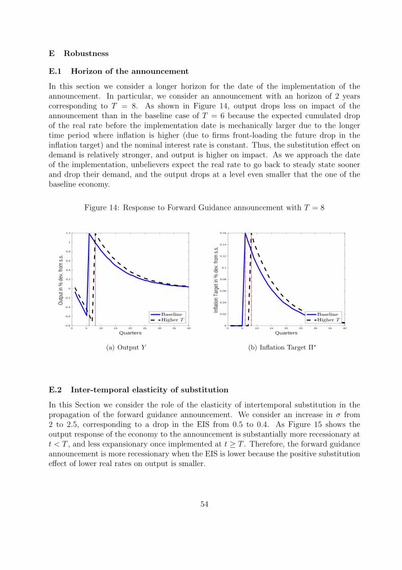
E Robustness

E.1 Horizon of the announcement

In this section we consider a longer horizon for the date of the implementation of theannouncement. In particular, we consider an announcement with an horizon of 2 yearscorresponding to T = 8. As shown in Figure 14, output drops less on impact of theannouncement than in the baseline case of T = 6 because the expected cumulated dropof the real rate before the implementation date is mechanically larger due to the longertime period where inflation is higher (due to firms front-loading the future drop in theinflation target) and the nominal interest rate is constant. Thus, the substitution effect ondemand is relatively stronger, and output is higher on impact. As we approach the dateof the implementation, unbelievers expect the real rate to go back to steady state soonerand drop their demand, and the output drops at a level even smaller that the one of thebaseline economy.

Figure 14: Response to Forward Guidance announcement with T = 8

0 5 10 15 20 25 30 35 40

Quarters

-0.8

-0.6

-0.4

-0.2

0

0.2

0.4

0.6

0.8

1

1.2

Out

put i

n %

dev

. fro

m s

.s.

BaselineHigher T

(a) Output Y

0 5 10 15 20 25 30 35 40

Quarters

0

0.02

0.04

0.06

0.08

0.1

0.12

0.14

0.16

Infla

tion

Targ

et in

% d

ev. f

rom

s.s

.

BaselineHigher T

(b) Inflation Target Π∗

E.2 Inter-temporal elasticity of substitution

In this Section we consider the role of the elasticity of intertemporal substitution in thepropagation of the forward guidance announcement. We consider an increase in σ from2 to 2.5, corresponding to a drop in the EIS from 0.5 to 0.4. As Figure 15 shows theoutput response of the economy to the announcement is substantially more recessionary att < T , and less expansionary once implemented at t ≥ T . Therefore, the forward guidanceannouncement is more recessionary when the EIS is lower because the positive substitutioneffect of lower real rates on output is smaller.

54

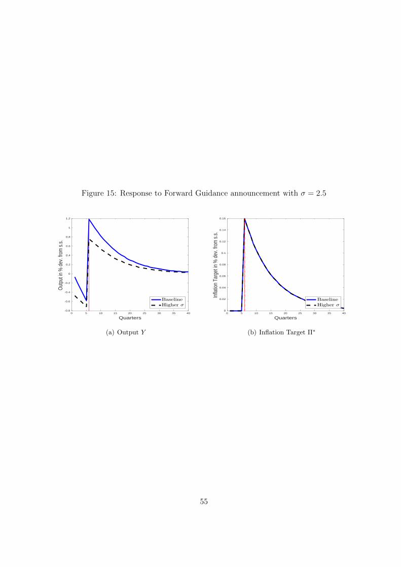
Figure 15: Response to Forward Guidance announcement with σ = 2.5

0 5 10 15 20 25 30 35 40

Quarters

-0.8

-0.6

-0.4

-0.2

0

0.2

0.4

0.6

0.8

1

1.2

Out

put i

n %

dev

. fro

m s

.s.

BaselineHigher <

(a) Output Y

0 5 10 15 20 25 30 35 40

Quarters

0

0.02

0.04

0.06

0.08

0.1

0.12

0.14

0.16In

flatio

n Ta

rget

in %

dev

. fro

m s

.s.

BaselineHigher <

(b) Inflation Target Π∗

55