ioapuoD

n

Altitude range resolutionof differential absorption lidar ozone profiles

Georg Beyerle and I. Stuart McDermid

A method is described for the empirical determination of altitude range resolutions of ozone profilesobtained by differential absorption lidar ~DIAL! analysis. The algorithm is independent of the imple-mentation of the DIAL analysis, in particular of the type and order of the vertical smoothing filter applied.An interpretation of three definitions of altitude range resolution is given on the basis of simulationscarried out with the Jet Propulsion Laboratory ozone DIAL analysis program, SO3ANL. These defini-tions yield altitude range resolutions that differ by as much as a factor of 2. It is shown that the altituderesolution calculated by SO3ANL, and reported with all Jet Propulsion Laboratory lidar ozone profiles,corresponds closely to the full width at half-maximum of a retrieved ozone profile if an impulse functionis used as the input ozone profile. © 1999 Optical Society of America

OCIS codes: 010.3640, 010.4950, 280.1910, 280.3640, 350.5730.

affi

r

1. Introduction

Differential absorption lidars ~DIAL’s! have been andcontinue to be widely used for the remote detectionand monitoring of atmospheric trace gases such asozone; see, e.g., Refs. 1–4. They now constitute anintegral part of the Network for the Detection ofStratospheric Change ~NDSC! for the long-term mon-toring of stratospheric ozone. To achieve the goalsf the NDSC, the ozone profiles supplied to the NDSCrchive have been extensively verified in intercom-arison campaigns; see, e.g., Refs. 5–7. However,ncertainty exists with respect to the interpretationf altitude resolutions reported by various ozoneIAL instruments.In routine DIAL analysis, ozone number densities

O3~z! are calculated by

nO3~z! 5

1sn 2 sf

H12F d

dzln

Pf~z!

Pn~z!G 2 @an~z! 2 af~z!#J ,

(1)

The authors are with the Table Mountain Facility, Jet Propul-sion Laboratory, California Institute of Technology, P. O. Box 367,Wrightwood, California 92397. G. Beyerle is also affiliated withthe Alfred Wegener Institute for Polar and Marine Research, Post-fach 600 149, D-14401 Potsdam, Germany. The authors’ emailaddresses are beyerle@tmf.jpl.nasa.gov and mcdermid@tmf.jpl.nasa.gov.

Received 4 May 1998; revised manuscript received 3 November1998.

0003-6935y99y060924-04$15.00y0© 1999 Optical Society of America

924 APPLIED OPTICS y Vol. 38, No. 6 y 20 February 1999

provided that the contribution from aerosol scatter-ing can be neglected.3,8,9 Here z is the geometricaltitude; for on and off wavelengths ln and lf, Pn~z!and Pf ~z! are the lidar signal counts at ln and lf, snand sf are the ozone absorption cross sections, and anand af are the extinction coefficients for molecularscattering at ln and lf, respectively.

The evaluation of the term dydz ln@Pf ~z!yPn~z!# isn essential element of the analysis. Generally, dif-erentiation has the effect of applying a high-passlter to a signal.10 In DIAL analysis this fact rep-

resents a problem, as the signal counts Pn,f ~z! atstratospheric altitudes contain high-wave-numbernoise contributions. A straightforward replacement

ddz

f ~z! 3fi11 2 fi21

zi11 2 zi21or

ddz

f ~z! 3fi 2 fi21

zi 2 zi21(2)

would therefore amplify detector and statistical noisecontributions more than the low-wave-number signalcomponents that are due to ozone absorption andrender the retrieved ozone profile useless.

Therefore stratospheric ozone DIAL algorithms, inmost cases, employ a derivative smoothing filter thatcuts off the high-frequency part of Pn,f ~z!:

ddz

lnPf~zi!

Pn~zi!3 (

j52N~i!

N~i!

cj~zi!lnPf~zi1j!

Pn~zi1j!, (3)

where cj denote the filter coefficients of the derivativefilter with order M 5 2N 1 1. As signal-to-noiseatios decrease for increasing altitude, the filter order

ES

b

Hn

ecwL

prk

and the filter coefficients are usually altitude depen-dent. A variety of different derivative filters havebeen described in the literature; see, e.g., Refs. 9 and11–13.

Typically, the altitude resolution dz~zi! of ozoneprofiles is defined in terms of the derivative filter.Because various filters are used, values of dz~zi! fromdifferent data analyses are generally not comparable.Here we propose an empirical approach to determin-ing dz~zi! that is independent of the particular filterused in the analysis program and can thus be appliedto any DIAL analysis. The method is illustratedwith simulations performed by SO3ANL, the Jet Pro-pulsion Laboratory’s stratospheric ozone DIAL anal-ysis program. SO3ANL analyzes two pairs ofsignals, Pn,f

L ~z! and Pn,fH ~z!. Superscript L refers to

the low-sensitivity channels ~L channels! for ozoneretrieval from 15 to 25 km, and superscript H tohigh-sensitivity channels ~H channels! for altitudesfrom 25 to 50 km.

In SO3ANL a polynomial derivative filter of degree1 is used; i.e., the filter coefficients are given by

cj 53j

N~N 1 1!~2N 1 1!, j 5 2N, . . . , N. (4)

On the basis of extensive simulations the altitudedependence of the filter order M 5 2N 1 1 is param-eterized as

ML 5 2(max$1.9396, 0.1871

3 exp@9.1 3 1025 m21~z 2 zs!#%1.046) 1 1,

MH 5 2(max$1.9396, 0.3741

3 exp@9.1 3 1025 m21~z 2 zs!#%1.046) 1 1

for the H ~subscript H! and the L ~subscript L! chan-nels, respectively, zs denotes the site altitude, and theboldface parentheses indicate rounding to the nearestinteger.

2. Altitude Resolution

We determined the altitude resolution by performinga DIAL analysis with a simulated raw-data profileconsisting of 1024 count values corresponding to the1024 multichannel–scaler bins of the Jet PropulsionLaboratory stratospheric ozone lidar data-acquisitionhardware. The detection channels operate in thephoton-counting mode. The dwell time for each binis 2 ms ~corresponding to a step height of Dz 5 300 m!.

ach simulated signal count profile was analyzed byO3ANL in the same manner as for real data.Two types of synthetic ozone profile, nin and nin,

were used. One, nin, is a sine wave with wave num-er k and phase 0 # w , 2p:

njin~zi! 5

A2

sin~2pkjzi 1 w! 1A2

, (5)

where A 5 1013 cm23. Adding the term Ay2 ensuresthat nj

in~zi! $ 0. The other, nin, is an impulse func-tion:

njin~zi! 5 HA zi 5 zj

0 else . (6)

In what follows njout~zi!@nj

out~zi!# denotes the resultobtained by SO3ANL for the synthetic input profilenj

in~zi!@njin~zi!#. As an illustration, Fig. 1 shows

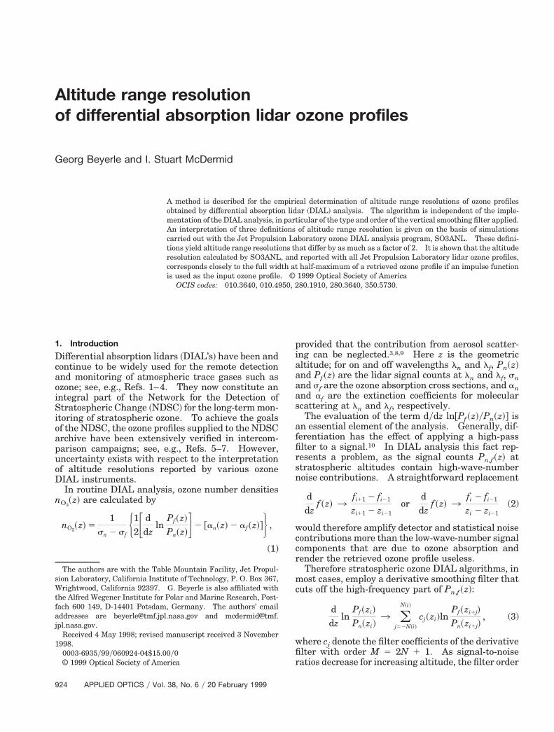
njout~zi! for three altitudes, zj 5 15 km, zj 5 25 km,

and zj 5 35 km, analyzed as L-channel data ~left! and-channel data ~right!. For clarity the figure doesot show the maximum of nj

in~zi! ~1013 cm23!. Ar-rows indicate the full width at half-maximum of theresults from the H- and L-channel analysis. Thevident asymmetry of the zj 5 35 km profiles isaused by the exponential increase of filter order Mith altitude. We note that in practice at 35 km the-channel analysis data are not used.Figure 2 shows nj

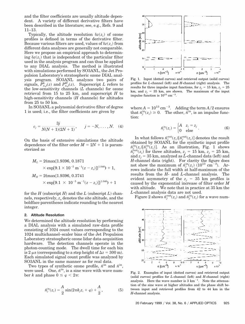
out~zi! and njin~zi! for a wave num-

Fig. 1. Input ~dotted curves! and retrieved output ~solid curves!rofiles for L-channel ~left! and H-channel ~right! analysis. Theesults for three impulse input functions, for zj 5 15 km, zj 5 25m, and zj 5 35 km, are shown. The maximum of the input

impulse function is 1013 cm23.

Fig. 2. Examples of input ~dotted curves! and retrieved output~solid curves! profiles for L-channel ~left! and H-channel ~right!analysis. Here the wave number is 3 km21. Note the attenua-tion of the sine wave at higher altitudes and the phase shift be-tween input and retrieved profiles from 42 to 44 km in theH-channel analysis.

20 February 1999 y Vol. 38, No. 6 y APPLIED OPTICS 925

m

Fi

ft

0

i

~otSs

9

ber of 3 km21. From 41- to 43-km altitude theH-channel data ~dashed curve, right! nj

out~zi! exhibita phase shift of p with respect to nj

in~zi!. The causefor this phase shift is discussed below.

In what follows, we investigate three ways to cal-culate the altitude resolution dz that are used inDIAL algorithms9,12,14,15:

~1! dz~1! 5 1yk1y2, where k1y2 is the wave number forwhich the response function drops to 50%; i.e., R~k1y2!5 1y2.

~2! dz~2! 5 M Dz, where Dz 5 zj11 2 zj is the stepheight.

~3! dz~3!, which is given by the full width at half-aximum of the retrieved profile nj

out~zi! if an im-pulse function nj

in~zi! is used as input.

As is shown below, these three definitions yield re-sults that differ by as much as a factor of 2.

3. Results and Discussion

A total of 1651 simulated count profiles were ana-lyzed by SO3ANL. For clarity no additional noisewas added to Pn,f ~z!. However, inasmuch asSO3ANL expects integer values for the signal counts,the simulated values Pn,f ~z! were rounded to thenearest integer, thereby producing quantizationnoise. One hundred fifty-one calculations weremade with an impulse function with zj, the location ofthe impulse, from 15 to 60 km and in steps of 300 m.One thousand five hundred simulations were per-formed with sine wave input profiles with wave num-bers of 1y300, 1y600, and 1y900 m21, etc., decreasingto 1y45,000 m21. For each wave number, ten pro-files with a random phase shift from 0 to 2p @relation~2!# were analyzed.

First we consider the sine input functions njin~zi!.

or njin~zi! we define a response function R by divid-

ng the derived and input ozone profiles:

R~kj, zi! 5nj

out~zi!

njin~zi!

. (7)

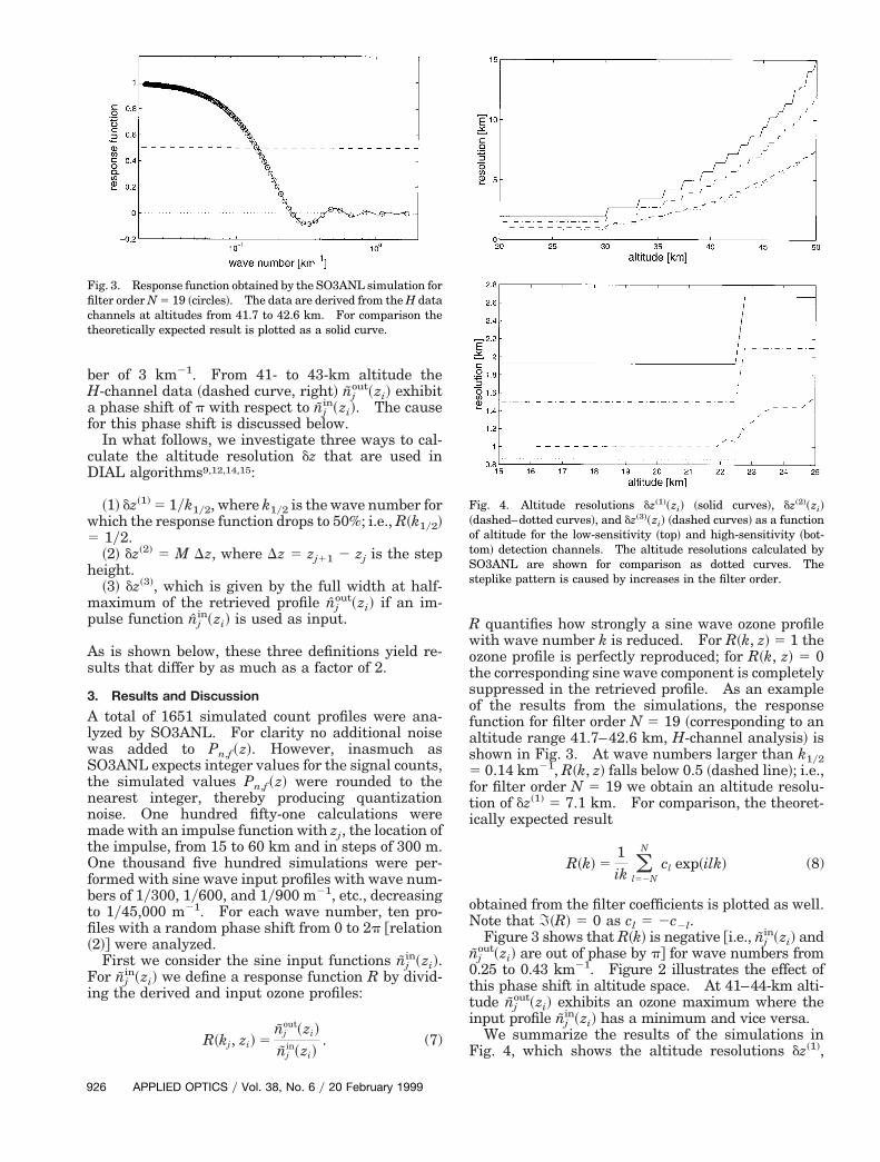
Fig. 3. Response function obtained by the SO3ANL simulation forfilter order N 5 19 ~circles!. The data are derived from the H datachannels at altitudes from 41.7 to 42.6 km. For comparison thetheoretically expected result is plotted as a solid curve.

26 APPLIED OPTICS y Vol. 38, No. 6 y 20 February 1999

R quantifies how strongly a sine wave ozone profilewith wave number k is reduced. For R~k, z! 5 1 theozone profile is perfectly reproduced; for R~k, z! 5 0the corresponding sine wave component is completelysuppressed in the retrieved profile. As an exampleof the results from the simulations, the responsefunction for filter order N 5 19 ~corresponding to analtitude range 41.7–42.6 km, H-channel analysis! isshown in Fig. 3. At wave numbers larger than k1y25 0.14 km21, R~k, z! falls below 0.5 ~dashed line!; i.e.,or filter order N 5 19 we obtain an altitude resolu-ion of dz~1! 5 7.1 km. For comparison, the theoret-

ically expected result

R~k! 51ik (

l52N

N

cl exp~ilk! (8)

obtained from the filter coefficients is plotted as well.Note that I~R! 5 0 as cl 5 2c2l.

Figure 3 shows that R~k! is negative @i.e., njin~zi! and

njout~zi! are out of phase by p# for wave numbers from.25 to 0.43 km21. Figure 2 illustrates the effect of

this phase shift in altitude space. At 41–44-km alti-tude nj

out~zi! exhibits an ozone maximum where thenput profile nj

in~zi! has a minimum and vice versa.We summarize the results of the simulations in

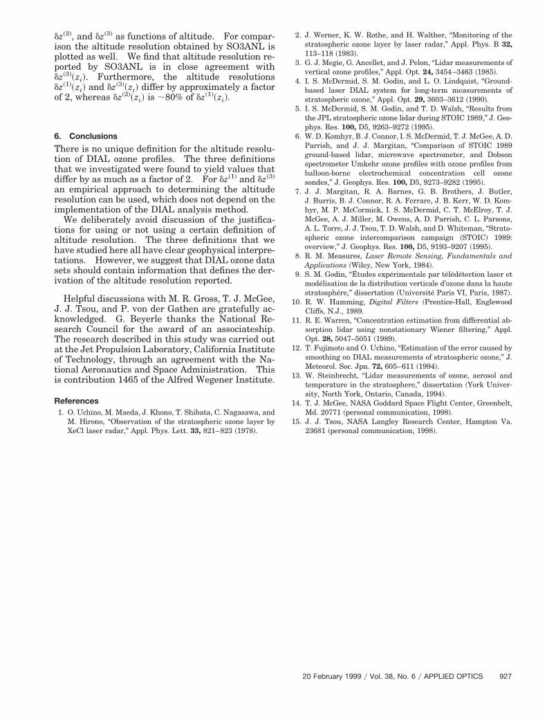
Fig. 4, which shows the altitude resolutions dz~1!,

Fig. 4. Altitude resolutions dz~1!~zi! ~solid curves!, dz~2!~zi!dashed–dotted curves!, and dz~3!~zi! ~dashed curves! as a functionf altitude for the low-sensitivity ~top! and high-sensitivity ~bot-om! detection channels. The altitude resolutions calculated byO3ANL are shown for comparison as dotted curves. Theteplike pattern is caused by increases in the filter order.

~2! ~3!

ippd

2. J. Werner, K. W. Rothe, and H. Walther, “Monitoring of the

dz , and dz as functions of altitude. For compar-son the altitude resolution obtained by SO3ANL islotted as well. We find that altitude resolution re-orted by SO3ANL is in close agreement withz~3!~zi!. Furthermore, the altitude resolutions

dz~1!~zi! and dz~3!~zi! differ by approximately a factorof 2, whereas dz~2!~zi! is ;80% of dz~1!~zi!.

6. Conclusions

There is no unique definition for the altitude resolu-tion of DIAL ozone profiles. The three definitionsthat we investigated were found to yield values thatdiffer by as much as a factor of 2. For dz~1! and dz~3!

an empirical approach to determining the altituderesolution can be used, which does not depend on theimplementation of the DIAL analysis method.

We deliberately avoid discussion of the justifica-tions for using or not using a certain definition ofaltitude resolution. The three definitions that wehave studied here all have clear geophysical interpre-tations. However, we suggest that DIAL ozone datasets should contain information that defines the der-ivation of the altitude resolution reported.

Helpful discussions with M. R. Gross, T. J. McGee,J. J. Tsou, and P. von der Gathen are gratefully ac-knowledged. G. Beyerle thanks the National Re-search Council for the award of an associateship.The research described in this study was carried outat the Jet Propulsion Laboratory, California Instituteof Technology, through an agreement with the Na-tional Aeronautics and Space Administration. Thisis contribution 1465 of the Alfred Wegener Institute.

References1. O. Uchino, M. Maeda, J. Khono, T. Shibata, C. Nagasawa, and

M. Hirono, “Observation of the stratospheric ozone layer byXeCl laser radar,” Appl. Phys. Lett. 33, 821–823 ~1978!.

stratospheric ozone layer by laser radar,” Appl. Phys. B 32,113–118 ~1983!.

3. G. J. Megie, G. Ancellet, and J. Pelon, “Lidar measurements ofvertical ozone profiles,” Appl. Opt. 24, 3454–3463 ~1985!.

4. I. S. McDermid, S. M. Godin, and L. O. Lindquist, “Ground-based laser DIAL system for long-term measurements ofstratospheric ozone,” Appl. Opt. 29, 3603–3612 ~1990!.

5. I. S. McDermid, S. M. Godin, and T. D. Walsh, “Results fromthe JPL stratospheric ozone lidar during STOIC 1989,” J. Geo-phys. Res. 100, D5, 9263–9272 ~1995!.

6. W. D. Komhyr, B. J. Connor, I. S. McDermid, T. J. McGee, A. D.Parrish, and J. J. Margitan, “Comparison of STOIC 1989ground-based lidar, microwave spectrometer, and Dobsonspectrometer Umkehr ozone profiles with ozone profiles fromballoon-borne electrochemical concentration cell ozonesondes,” J. Geophys. Res. 100, D5, 9273–9282 ~1995!.

7. J. J. Margitan, R. A. Barnes, G. B. Brothers, J. Butler,J. Burris, B. J. Connor, R. A. Ferrare, J. B. Kerr, W. D. Kom-hyr, M. P. McCormick, I. S. McDermid, C. T. McElroy, T. J.McGee, A. J. Miller, M. Owens, A. D. Parrish, C. L. Parsons,A. L. Torre, J. J. Tsou, T. D. Walsh, and D. Whiteman, “Strato-spheric ozone intercomparison campaign ~STOIC! 1989:overview,” J. Geophys. Res. 100, D5, 9193–9207 ~1995!.

8. R. M. Measures, Laser Remote Sensing, Fundamentals andApplications ~Wiley, New York, 1984!.

9. S. M. Godin, “Etudes experimentale par teledetection laser etmodelisation de la distribution verticale d’ozone dans la hautestratosphere,” dissertation ~Universite Paris VI, Paris, 1987!.

10. R. W. Hamming, Digital Filters ~Prentice-Hall, EnglewoodCliffs, N.J., 1989.

11. R. E. Warren, “Concentration estimation from differential ab-sorption lidar using nonstationary Wiener filtering,” Appl.Opt. 28, 5047–5051 ~1989!.

12. T. Fujimoto and O. Uchino, “Estimation of the error caused bysmoothing on DIAL measurements of stratospheric ozone,” J.Meteorol. Soc. Jpn. 72, 605–611 ~1994!.

13. W. Steinbrecht, “Lidar measurements of ozone, aerosol andtemperature in the stratosphere,” dissertation ~York Univer-sity, North York, Ontario, Canada, 1994!.

14. T. J. McGee, NASA Goddard Space Flight Center, Greenbelt,Md. 20771 ~personal communication, 1998!.

15. J. J. Tsou, NASA Langley Research Center, Hampton Va.23681 ~personal communication, 1998!.

20 February 1999 y Vol. 38, No. 6 y APPLIED OPTICS 927