Alternative DRM formulations

Wang, K.; Mattheij, R.M.M.; ter Morsche, H.G.

Published: 01/01/2002

Document VersionPublisher’s PDF, also known as Version of Record (includes final page, issue and volume numbers)

Please check the document version of this publication:

• A submitted manuscript is the author's version of the article upon submission and before peer-review. There can be important differencesbetween the submitted version and the official published version of record. People interested in the research are advised to contact theauthor for the final version of the publication, or visit the DOI to the publisher's website.• The final author version and the galley proof are versions of the publication after peer review.• The final published version features the final layout of the paper including the volume, issue and page numbers.

Link to publication

General rightsCopyright and moral rights for the publications made accessible in the public portal are retained by the authors and/or other copyright ownersand it is a condition of accessing publications that users recognise and abide by the legal requirements associated with these rights.

• Users may download and print one copy of any publication from the public portal for the purpose of private study or research. • You may not further distribute the material or use it for any profit-making activity or commercial gain • You may freely distribute the URL identifying the publication in the public portal ?

Take down policyIf you believe that this document breaches copyright please contact us providing details, and we will remove access to the work immediatelyand investigate your claim.

Download date: 17. Jul. 2018

EINDHOVEN UNIVERSITY OF TECHNOLOGYDepartment of Mathematics and Computing Science

RANA02-03January 2002

Alternative DRM formulations

by

K. Wang, R.M.M. Mattheij and H.G. ter Morsche

Reports on Applied and Numerical AnalysisDepartment of Mathematics and Computing ScienceEindhoven University of TechnologyP.O. Box 5135600 MB Eindhoven, The NetherlandsISSN: 0926-4507

Alternative DRM formulations

K. Wang, R.M.M. Mattheij & H.G.ter MorscheDepartment ofMathematics and Computing Science,Eindhoven University ofTechnology,Po. Box 513,5600 MB Eindhoven, The Netherlands

Abstract

In this paper, we present two DRM formulations. For a pseudo-Poisson equa­tion, if the right hand side is a linear operation on the dependent variable, we canderive a new DRM formulation. In comparison with the traditional DRM formu­lation for the same equation, the new one is much easier and more efficient. Forthe axisymmetric Poisson equation, we construct a DRM formalation by usingthe linear axisymmetric radial basis function. The particular solution involved iswritten in a closed form, and thus speeds up the evaluation of the particular solu­tion. A few numerical examples demonstrate the accuracy and efficiency of theseformulations.

1 Introduction

The boundary element method (BEM) is now a powerful alternative numericaltechnique for solving partial differential equations (PDEs). For homogeneousPDEs, only the boundary discretisation is necessary. For inhomogeneous PDEs,however, the integral equation involves domain integrals. To avoid domain inte­grals, the dual reciprocity method (DRM) was proposed [5]. This method actuallydivides the solution into two parts: a particular solution of the inhomogeneousPDE plus a solution of its homogeneous counterpart. Since particular solutions

I

to complex inhomogeneities are very difficult or even impossible to obtain, theinhomogeneity is normally represented by a series expansion in terms of simplerfunctions for which particular solutions can be (easily) determined [11]. Further­more, the DRM has been extended to deal with nonlinear problems, heterogeneousproblems, variable coefficient problems and time-dependent problems.

In this paper, we first consider the following equation

\72u = p(u), (1)

where p is a linear operator. This problem has been addressed in [5], but wewill present a new formulation which turns out to be easier and more efficient.We have to say something about the type of equation (1). Since p is a linearoperator with respect to u, one might hope to be able to find the fundamentalsolution to the (homogeneous) equation (1); however, this is normally difficult,even more when p(u) includes variable coefficients. To solve equation (1), wemay employ the fundamental solution for the Laplacian, and consider the problemas a Poisson-type equation. Therefore the right hand side p(u) may be regardedas an inhomogeneity or pseudo source.

Secondly we apply the dual reciprocity method to the following axisymmetricPoisson equation.

\7~u := Urr + ~Lr/r + Uzz = b, (2)

where b is a given function. Conceptually this is nothing special, but it is ex­tremely difficult to find a particular solution to the axisymmetric Laplacian for thetraditional radial basis functions (RBFs) being the right hand side. We turned tothe axisymmetric RBFs.

The paper is organised as follows: In Section 2, we recall the essentials ofthe DRM and show how equation (1) is solved by the DRM traditionally. A newformulation for equation (1) is derived in Section 3, which is better than the tra­ditionalone. In Section 4, an axisymmetric DRM formulation is established forequation (2). A few numerical examples are shown in Section 5. Comments andconclusions are given in Section 6.

2 The basic DRM

In this section we briefly recall the essentials of the DRM. We start with theLaplace equation. Consider a domain n with boundary r and let u satisfy

\72u = O. (3)

2

Then the integral equation corresponding to (3) is

c(x)u(x) + Ir q*udf = Ir qu*df, (4)

where c(x) is a function of position; u* and q* are the fundamental solution andits nonnal derivative; q is the nonnal derivative of u.

We subdivide the boundary f into boundary elements by N nodes {Xl, ... ,XN},and if we have L points {XN+l"" ,xN+d inside n for which the values of ushould be evaluated, then the BEM discretised version for (4) reads

Hu - Gq = 0, (5)

where u := (U(XI),'" ,u(xN+L)f, q := (q(XI),'" ,q(XN)f. The matrices Hand G have the following structure

(6)

where HI and G I are N x N matrices, H 2 and G 2 are L x N matrices, I is anL x L unit matrix.

we deliberately put two uncoupled equations in the fonn (5) to make the writ­ing simpler when we talk about the DRM late.

2.1 DRM for Poisson equations

Consider a simple source tenn for the Poisson equation

\72u = b, (7)

where b is some smooth function of x.To solve this equation, b is first approximated in tenns·ofa set of (radial) basis

functions {</>j}

N+Lb(x) == L ajC/Jj(x).

j

To detennine the coefficients aj, we use interpolation, i.e.

N+Lb(Xi) = L ajC/)j(xi), i = 1,'" ,N + L.

j

3

(8)

(9)

In matrix form, this reads

Fa=b, (10)

where b := (b(Xl),'" ,b(XN+L)f, a := (001,'" ,aN+Lf and the matrix F isdefined by its elements <Pj(Xi)'

We are interested in such <Pj that it is easy to find a particular solution Uj forwhich

This implies that

N+Lu(x) = L ajuj(x),

j

(11)

(12)

is an approximate particular solution to equation (7), i.e., u - {I approximatelysatisfies the Laplace equation

From the standard BEM (see (5)) we have

H(u - u) - G(q - q) = 0,

l.e.

Hu - Gq = Hu - Gq,

where u and q are defined similarly to u and q respectively.From (12), we can easily see that

u=Ua, q=Qa,

where the matrices Uand Q are (Uj(Xi)) and (t]j(Xi)) respectively.By plugging (16) into (15) and using (10) we finally arrive at

Hu - Gq = (HU - GQ)F-lb.

This is the pith and marrow of the DRM.

4

(13)

(14)

(15)

(16)

(17)

2.2 DRM for pseudo-Possion equations

It is possible to generalise the foregoing to right hand sides which depend on theunknown

(18)

where p is a linear operator. Before we give our alternative approach in section 3,we first show how this kind of problem has been solved in [5].

Define the vector p:= [P(U)(Xl), ... ,p(U) (XN+L)jT. Using equation (17),we obtain

(19)

Now, in order to solve equation (19), the unknown p should be represented by u(and/or q). To this end, U is expanded in terms of {q)j}

N+Lu(x) == L Ctjq)j(x).

j

Subsequently we get

N+Lp(u)(x) == L Ctjp(q)j)(x).

j

By using interpolation in (20) and (21), we obtain

(20)

(21)

N+L N+LU(Xi) = L Ctjq)j(Xi),p(U)(Xi) = L Ctjp(q)j)(Xi) , i =1,'" ,N + L. (22)

j j

Rewriting (22) in matrix form gives

(23)

where F1 denotes the matrix (P(q)j) (Xi))' From (23) we find that p is given by

p = F1F-1u. (24)

We now substitute this representation into (19) and obtain the system

Hu - Gq = (HU - GQ)F-1F1F-1u,

from which u and q can be found after applying the boundary condition(s).

5

(25)

3 An easier DRM formulation

The main idea of the DRM is to expand the right hand side to find an approximateparticular solution.

If we could find particular solutions Uj, such that

\72Uj (X) = p(cPj)(X) , j = 1,··· , N + L,

then we see from (20) and (21) that

N+L

u(x) := L ajuj(x),j

satisfies

i.e., u - U satisfies Laplace's equation. Consequently, by using (5) we obtain

Hu - Gq = Hfi. - Gq.

(26)

(27)

(28)

(29)

Define matrices V ij = (uj(xd) and Qij = (ijj(xd). Performing the samemanipulations as in Section 2.1, we get a more elegant computational scheme

Hu - Qq = (HV - GQ)F-1u. (30)

Comparing (30) with (25), we can see (30) is easier and more efficient than(25). Scheme (30) looks more like (17), the difference is that U and Q are re­placed by V and Q respectively. While scheme (25) looks a bit more complicated.

Remark 1. We can see that, the essential difference between this new approachand the traditional DRM is that the new approach uses the particular solutions Uj

while the traditional DRM uses the particular solutions Uj

\72Uj = cPj'

(31)

(32)

For radial basis functions (RBFs) [7], Uj are always available for the Laplacian,but the availability of Uj depends on the operator p. If it is really difficult to findUj, then we can choose {cPj} such that p(cPj) are REFs. In this way, Uj is alsonearly always available.

6

Remark 2. For the case p(u) = cu (c is a constant), it is obvious that scheme(30) and (25) result in the same set of linear equations since F1 = cF and Uj =CUj'

4 An axisymmetric DRM formulation

The major problem here is to find a particular solution Uj for a given basis functioncPj (e.g. a radial basis function), satisfying

(33)

This is not a trivial task. To circumvent this problem, one may start with a givenUj and then compute cPj by differentiation. For example, in [10] the particularsolution is chosen to be Uj = dJ/12; therefore the basis function is then cPj =dj (l - rj/4r). In [4], Uj = rj(Cd] + r 3a;) and cPj = rj(C(12 - 3rj/r)dj ­14rjT2 + 9rdJ + 18r3 ). We can see that the choice of Uj is rather arbitrary andlacks mathematical foundation. Another weak point of these two methods is thatcPj is not defined at r = O.

Here we develop a simple and logical method which enables us to find theanalytical expression for both Uj and cPj satisfying (33). The idea is to use athree-dimensional particular solution and integrate it with respect to () from 0 to21r. This method has been explored in [6] for the Helmholtz equation. in that case,Uj is expressed by an integral. Fortunately, for the Laplacian we are able to deriveUj in a closed form, at least for the linear RBF.

In the three-dimensional case we know that uj = ~ satisfies

Rewriting this equation in the cylindrical coordinates (r, 0, z) gives

1 02-1 l:l2-1 1l:l-1 l:l2-1Uj U Uj UUj U Uj _ dr 2 oOZ + or2 +;: or + 0Z2 - j'

Integrating the above equation, we obtain

l:l2- 1l:l- l:l2-~+_UUj +~ = cP',or2 r or oz2 J

7

(34)

(35)

(36)

where

(37)

and

Uj =127r

~~df) = ~(a + b)va+b((k2 - l)K(k) + (4 - 2k2)E(k)) 0 (38)

Here a := rJ + r2+ (Zj - z)2, b := 2rjr, k := J2b/(a + b); K and E are thecomplete elliptic function of the first kind and second kind, respectively. The firstorder derivatives of Uj are

00- ~- ( )a: = (r + rj)vla + bE(k) + 3k~ via + b (k2 - l)K(k) + (1 - 2k2)E(k) ,

(39)

and

au-a: = (z - zj)vla + bE(k). (40)

It is easy to verify that ¢>j, Uj, ~ and ~ are all continuous in the whole domain{(r,z) I r ~ 0,-00 < Z < oo}.

In [6], the author has numerically shown the local property of ¢>jo This isimportant when the function to be interpolated varies steeply over the domain.

5 Numerical examples

In this section, we demonstrate some numerical examples.

5.1 A convection-diffusion problem

As a first application, let us investigate a steady 2D convection-diffusion problemin Cartesian coordinates

(41)

8

where u is the quantity being convected, Vl and V2 are the velocity components,and K is the diffusivity. Combining Vl, V2 and K into parameters a and b respec­tively, we obtain

2 au au\7 u = aax + bay .

We assume here that a and b are both constant.In this case, p = a tx + btv 0 Our task is to find Uj such that

~2-. _ acPi ba¢jv uJ - a ax + ay'

(42)

(43)

for each ¢joIt is easy to verify (although maybe less easy to find) that, for the linear radial

basis function

¢j := dj ,

with dj = J(x - Xj)2 + (y - Yj)2, the particular solution is given by

Uj = (ax + by)dj /3.

For the thin plate spline

¢j:= d;ln(dj ),

the particular solution is

Uj = (ax + by)d;(41n(dj ) -1)/16.

(44)

(45)

(46)

(47)

For variable a and b, we can't expect that we can always find the particularsolutions Uj for commonly used RBFs. If this is the case, then remark 1 in theprevious section applies.

we consider a model problem in an oval domain (x2/4 + y2 < 1)

~u=-~ ~~ax

i.e. a = -1, b = O. the boundary condition is chosen such that the problem hasan exact solution u = exp(-x).

The boundary is subdivided into elements by 16 boundary points; moreoverwe also use 17 internal points as in [5] (see Figure 1). The values ofu at numberedpoints are shown in Table 1. The advantages of the new approach are obvious.

9

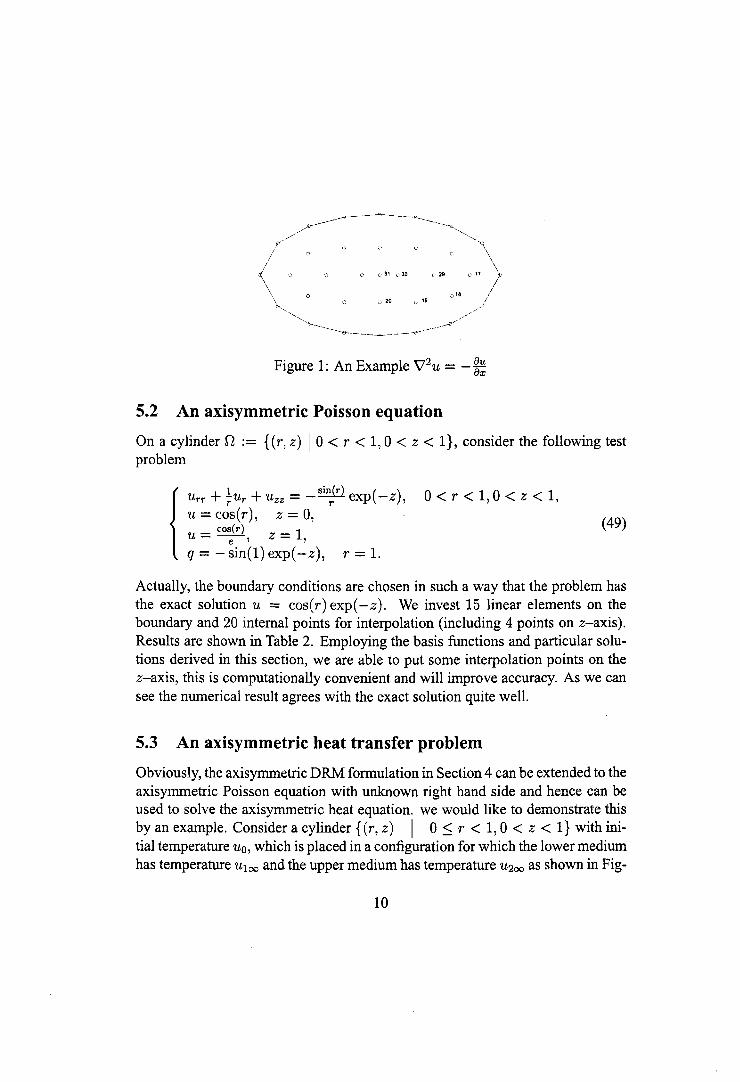
Figure 1: An Example V'2u = - ~~

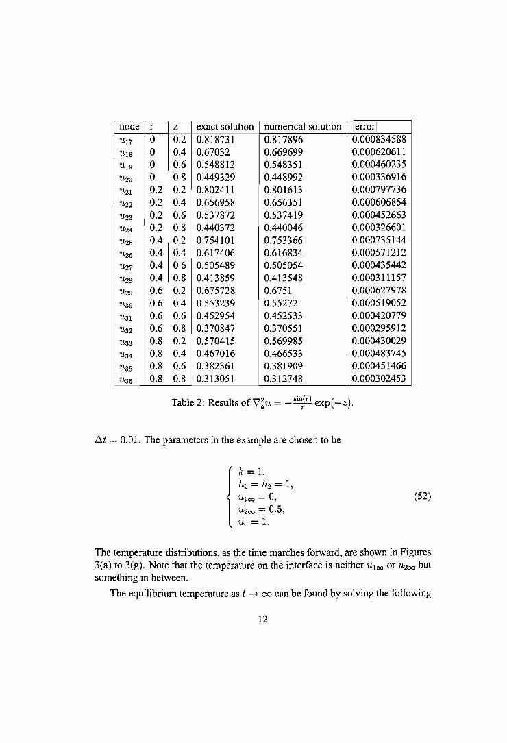
5.2 An axisymmetric Poisson equation

On a cylinder n := {(r, z) I 0 < r < 1, 0 < z < I}, consider the following testproblem

{

Urr + :ur + U zz = _sin;r) exp(-z),U = cos(r), z = 0,U = cos(r) Z = 1

e ' ,q = - sin(l) exp(-z), r = 1.

0< r < 1,0 < z < 1,

(49)

Actually, the boundary conditions are chosen in such a way that the problem hasthe exact solution U = cos(r)exp(-z). We invest 15 linear elements on theboundary and 20 internal points for interpolation (including 4 points on z-axis).Results are shown in Table 2. Employing the basis functions and particular solu·tions derived in this section, we are able to put some interpolation points on thez-axis, this is computationally convenient and will improve accuracy. As we cansee the numerical result agrees with the exact solution quite well.

5.3 An axisymmetric heat transfer problem

Obviously, the axisymmetric DRM formulation in Section 4 can be extended to theaxisymmetric Poisson equation with unknown right hand side and hence can beused to solve the axisymmetric heat equation. we would like to demonstrate thisby an example. Consider a cylinder {(r, z) I 0 ~ r < 1,0 < z < I} with ini­tial temperature un, which is placed in a configuration for which the lower mediumhas temperature Uloo and the upper medium has temperature U200 as shown in Fig-

10

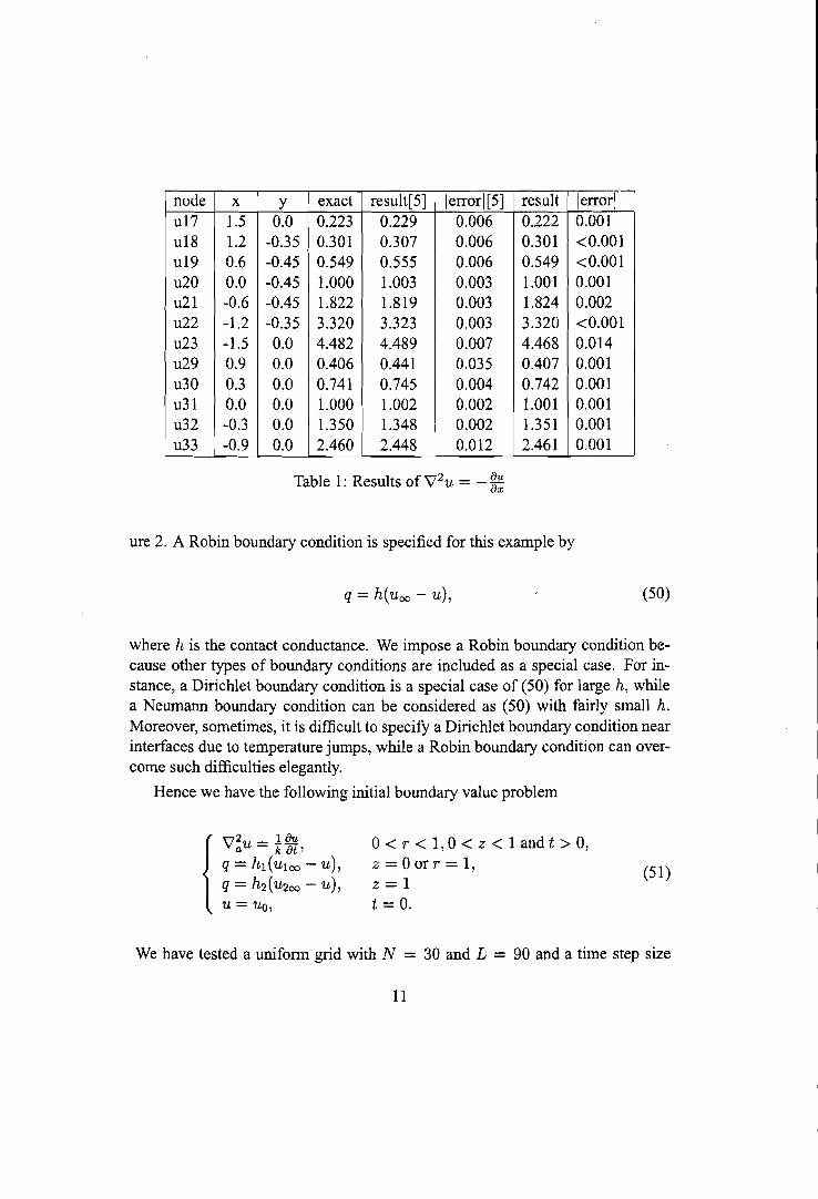
node x y exact result[5] [errorI[5] result Ierror Iu17 1.5 0.0 0.223 0.229 0.006 0.222 0.001ulS 1.2 -0.35 0.301 0.307 0.006 0.301. <0.001u19 0.6 -0.45 0.549 0.555 0.006 0.549 <0.001u20 0.0 -0.45 1.000 1.003 0.003 1.001 0.001u21 -0.6 -0.45 1.822 1.819 0.003 1.824 0.002u22 -1.2 -0.35 3.320 3.323 0.003 3.320 <0.001u23 -1.5 0.0 4.482 4.489 0.007 4.468 0.014u29 0.9 0.0 0.406 0.441 0.035 0.407 0.001u30 OJ 0.0 0.741 0.745 0.004 0.742 0.001u31 0.0 0.0 1.000 1.002 0.002 1.001 0.001u32 -OJ 0.0 1.350 1.348 0.002 1.351 0.001u33 -0.9 0.0 2.460 2.448 0.012 2.461 0.001

Table 1: Results of yr2u = - ~~

ure 2. A Robin boundary condition is specified for this example by

q = h(uoo - u), (50)

where h is the contact conductance. We impose a Robin boundary condition be­cause other types of boundary conditions are included as a special case. For in­stance, a Dirichlet boundary condition is a special case of (50) for large h, whilea Neumann boundary condition can be considered as (50) with fairly small h.Moreover, sometimes, it is difficult to specify a Dirichlet boundary condition nearinterfaces due to temperature jumps, while a Robin boundary condition can over­come such difficulties elegantly.

Hence we have the following initial boundary value problem

o< r < 1,°< z < 1 and t > 0,z = 0 or r = 1,z=lt = O.

(51)

We have tested a uniform grid with N = 30 and L = 90 and a time step size

11

node r z exact solution numerical solution Ierror I

Ul7 0 0.2 0.818731 0.817896 0.000834588

UI8 0 0.4 0.67032 0.669699 0.000620611

UI9 0 0.6 0.548812 0.548351 0.000460235

U20 0 0.8 0.449329 0.448992 0.000336916

U2I 0.2 0.2 0.802411 0.801613 0.000797736

U22 0.2 0.4 0.656958 0.656351 0.000606854

U23 0.2 0.6 0.537872 0.537419 0.000452663U24 0.2 0.8 0.440372 0.440046 0.000326601

U25 0.4 0.2 0.754101 0.753366 0.000735144

U26 0.4 0.4 0.617406 0.616834 0.000571212

U27 0.4 0.6 0.505489 0.505054 0.000435442

U28 0.4 0.8 0.413859 0.413548 0.000311157

U29 0.6 0.2 0.675728 0.6751 0.000627978

U30 0.6 0.4 0.553239 0.55272 0.000519052

U3I 0.6 0.6 0.452954 0.452533 0.000420779

U32 0.6 0.8 0.370847 0.370551 0.000295912

U33 0.8 0.2 0.570415 0.569985 0.000430029

U34 0.8 0.4 0.467016 0.466533 0.000483745

U35 0.8 0.6 0.382361 0.381909 0.000451466

U36 0.8 0.8 0.313051 0.312748 0.000302453

Table 2: Results of \7~,u = - sin;T) exp(-z).

l:i.t = 0.01. The parameters in the example are chosen to be

k = 1,hI = h2 = 1,Ul oo = 0,U200 = 0.5,Uo = 1.

(52)

The temperature distributions, as the time marches forward, are shown in Figures3(a) to 3(g). Note that the temperature on the interface is neither Uloo or U200 butsomething in between.

The equilibrium temperature as t -t 00 can be found by solving the following

12

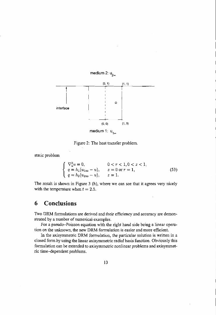
medium 2: u200

(0.1) (1, 1)

1

I

I

I

I

I nI

interface I

I

I

I

(0,0) (1, 0)

medium 1: u100

Figure 2: The heat transfer problem.

static problem

o< r < 1,0 < z < 1,z = 0 orr = 1,z=l.

(53)

The result is shown in Figure 3 (h), where we can see that it agrees very nicelywith the temperature when t = 2.5.

6 Conclusions

Two DRM formulations are derived and their efficiency and accuracy are demon­strated by a number of numerical examples.

For a pseudo-Poisson equation with the right hand side being a linear opera­tion on the unknown, the new DRM formulation is easier and more efficient.

In the axisymmetric DRM formulation, the particular solution is written in aclosed form by using the linear axisymmetric radial basis function. Obviously thisformulation can be extended to axisymmetric nonlinear problems and axisymmet­ric time-dependent problems.

13

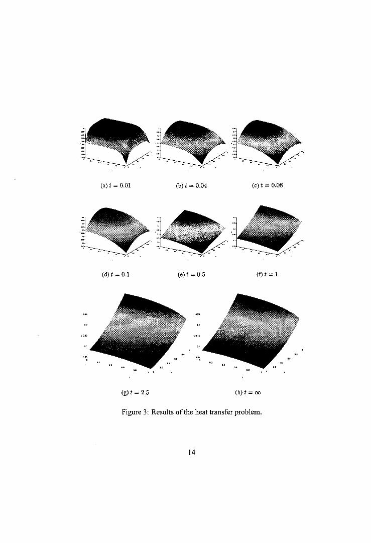
(a) t = 0.01

(d) t =0.1

(b) t =0.04

(e)t=0.5

(c) t = 0.08

(f) t = 1

'",

, ,

(g) t = 2.5

,.",

, '

(h) t = 00

Figure 3: Results of the heat transfer problem.

14

References

[1] Bakr A.A. The boundary integral equation method in axisymmetric stressanalysis problems. Springer-Verlag. 1986.

[2] Carslaw H.S. & Jaeger J.C. Conduction ofheat in solids. Oxford UniversityPress. 1959.

[3] Golberg M.A., Chen C.S., Bowman H. & Power H. Some comments on theuse ofradial basis functions in the dual reciprocity method. ComputationalMechanics 1998; 22: 61-69.

[4] Masse B. & Marcouiller L. Axisymmetricflow problems using the dual reci­procity boundary element method. Boundary Elements 14, 1992, pp.639­650.

[5] Partridge P.W., Brebbia C.A. & Wrobel L.c. The dual reciprocity boundaryelement method. Computational Mechanics Publications. 1992.

[6] Perrey-Debain, E. Analysis ofconvergence and accuracy ofthe DRBEMforaxisymmetric Helmholtz-type equation. Engineering analysis with bound­ary element methods 1999,23: 703-711.

[7] Powell M.J. The theory ofradial basis function approximation in 1990. In:Advances in numerical analysis. Vol. 2. Oxford University Press. 1992.

[8] Sarler Bozidar Axisymmetric augmented thin plate splines. EngineeringAnalysis with Boundary Elements 1998,21: 81-85.

[9] Surdo C.L. Generalized axisymmetric Poisson equation (GASPE): separa­ble cases and Green-Dirichlet problem in a circle. 1. Math. Anal. Appl.1976; 56: 477-491.

[10] Wrobel L.c. & Telles 1.c. & Brebbia C.A. A dual reciprocity boundary el­ementfomulation for axisymmetric diffusion problems. Boundary Elements8, 1986, pp.59-69.

[IIJ Yamada T. & Wrobel L.c. Properties ofGaussian radial basis functions inthe dual reciprocity boundary element method. Z angew Math. Phys. 1993;44: 1054-1067.

15