algorithmsforsaferobotnavigation brian maxim axelrod · algorithmsforsaferobotnavigation by...
TRANSCRIPT

Algorithms for Safe Robot Navigation
by Brian Maxim Axelrod
Submitted to theDepartment of Electrical Engineering and Computer Sciencein Partial Fulfillment of the Requirements for the Degree of
Master of Engineering in Electrical Engineering and Computer Scienceat the
Massachusetts Institute of TechnologySeptember 2017
c○ 2017 Brian Maxim Axelrod. All rights reserved.
The author hereby grants to MIT permission to reproduce and todistribute publicly paper and electronic copies of this thesis documentin whole or in part in any medium now known or hereafter created.
Author . . . . . . . . . . . . . . . . . . . . . . . . . . . . . . . . . . . . . . . . . . . . . . . . . . . . . . . . . . . . . . . .Department of Electrical Engineering and Computer Science
August 18, 2017Certified by. . . . . . . . . . . . . . . . . . . . . . . . . . . . . . . . . . . . . . . . . . . . . . . . . . . . . . . . . . . .
Leslie Pack KaelblingPanasonic Professor of Computer Science and Engineering
Thesis SupervisorCertified by. . . . . . . . . . . . . . . . . . . . . . . . . . . . . . . . . . . . . . . . . . . . . . . . . . . . . . . . . . . .
Tomás Lozano-PérezSchool of Engineering Professor in Teaching Excellence
Thesis SupervisorAccepted by . . . . . . . . . . . . . . . . . . . . . . . . . . . . . . . . . . . . . . . . . . . . . . . . . . . . . . . . . . .
Christopher J. TermanChairman, Department Committee on Graduate Theses

2

Algorithms for Safe Robot Navigation
by
Brian Maxim Axelrod
Submitted to the Department of Electrical Engineering and Computer Scienceon August 18, 2017, in partial fulfillment of the
requirements for the Degree ofMaster of Engineering in Electrical Engineering and Computer Science
Abstract
As drones and autonomous cars become more widespread it is becoming increasinglyimportant that robots can operate safely under realistic conditions. The noisy infor-mation fed into real systems means that robots must use estimates of the environmentto plan navigation. Efficiently guaranteeing that the resulting motion plans are safeunder these circumstances has proved difficult.
We build a mathematical framework for analyzing the quality of estimated geom-etry, rigorously developing the notion of shadows. We then examine how to use thesetools guarantee that a trajectory or policy is safe with only imperfect observationsof the environment. We present efficient algorithms that can prove that trajectoriesor policies are safe with much tighter bounds than in previous work. Notably, thecomplexity of the environment does not affect our method’s ability to evaluate if atrajectory or policy is safe.
We also examine the implications of various mathematical formalisms of safetyand arrive at a mathematical notion of safety of a long-term execution, even whenconditioned on observational information.
Thesis Supervisor: Leslie Pack KaelblingTitle: Panasonic Professor of Computer Science and Engineering
Thesis Supervisor: Tomás Lozano-PérezTitle: School of Engineering Professor in Teaching Excellence
3

4

Acknowledgments
First I must thank Leslie Pack Kaelbling and Tomás Lozano-Pérez. Ever since I joined
the Learning and Intelligent Systems group (LIS) four years ago they have dedicated
countless hours to mentoring me. They have advised me in research, academics, grad
school applications and life in general. They demonstrated incredible patience while
listening to explanations of my work, and asked questions that defined future work.
They always advocated on their students’ behalf to administration and fellowships
and always had our futures in mind. They welcomed us into their homes, expressed
concern over our well being, and made LIS feel like a family.
I also have to thank the rest of LIS. The graduate students were always open-
minded, curious and willing to talk with me about research, classes and life. They
were invaluable collaborators in many projects and classes. I would especially like
to thank Arial Anders, Rohan Chitnis, Caelan Garret, Patrick Barragan, Clement
Gehring and Gustavo Goretkin for sharing their offices with me. Those were good
times. Teresa Cataldo also deserves much credit for ensuring that we were always
well fed and travel and purchases went smoothly.
I would also like to thank my fellow residents of East Campus and 4E in partic-
ular. It wasn’t just a place of long nights helping each other, fun outings, awesome
construction projects, winning Green building challenges and looking out for each
other; it was the place that reminded me that all these geniuses around me have a
human side too.
I owe a lot of my mathematical development to Michael Artin and his incredible
dedication to teaching. He believed that we could become mathematicians regardless
of our background and spent countless hours helping us not only fill gaps in our
knowledge, but truly understand and think about the material like mathematicians.
Equally important are those who influenced me before I came to MIT. David Gi-
andomenico, Jon Penner, Steve Cousins and Kaijen Hsiao. The opportunities they
provided helped me develop intellectually and as an individual. My experiences work-
ing with them still color the way I view the world today.
5

Finally I would like to thank my parents for raising me in such a way that en-
couraged independence and challenging myself intellectually. They set an example of
determination and hard work that has, and continues to, inspire me every day.
6

Contents
1 Introduction 13
1.1 Motivation . . . . . . . . . . . . . . . . . . . . . . . . . . . . . . . . . 14
1.2 Related Work . . . . . . . . . . . . . . . . . . . . . . . . . . . . . . . 15
1.3 Contributions and Outline . . . . . . . . . . . . . . . . . . . . . . . . 16
2 Shadows 19
2.1 Mathematics of Shadows . . . . . . . . . . . . . . . . . . . . . . . . . 20
2.1.1 Definitions . . . . . . . . . . . . . . . . . . . . . . . . . . . . . 20
2.1.2 A characterization of half-space Shadows . . . . . . . . . . . . 23
2.2 Computing Shadows for PGDFs . . . . . . . . . . . . . . . . . . . . . 27
2.2.1 Gaussian Elliptical Shadows . . . . . . . . . . . . . . . . . . . 28
2.2.2 Conic Shadows . . . . . . . . . . . . . . . . . . . . . . . . . . 32
2.2.3 From Halfspaces to Polytopes . . . . . . . . . . . . . . . . . . 32
3 Algorithm for Bounding Probability of Collision 35
3.1 Motivation . . . . . . . . . . . . . . . . . . . . . . . . . . . . . . . . . 35
3.2 The Single Obstacle Case . . . . . . . . . . . . . . . . . . . . . . . . . 37
3.3 Generalization to Multiple Obstacles . . . . . . . . . . . . . . . . . . 38
3.4 Verification of Safety Certificates . . . . . . . . . . . . . . . . . . . . 41
4 Algorithms for Finding Safe Plans 43
4.1 Motivation . . . . . . . . . . . . . . . . . . . . . . . . . . . . . . . . . 43
4.2 A Probabilistically Complete Planner for Safe Motion Planning . . . 46
7

4.3 Hardness . . . . . . . . . . . . . . . . . . . . . . . . . . . . . . . . . . 48
5 Safety in the Online Setting 51
5.1 Motivation . . . . . . . . . . . . . . . . . . . . . . . . . . . . . . . . . 51
5.2 Absolute Safety . . . . . . . . . . . . . . . . . . . . . . . . . . . . . . 54
5.2.1 Absolute Safety vs traditional . . . . . . . . . . . . . . . . . . 56
5.2.2 Absolute Safety using Shadows . . . . . . . . . . . . . . . . . 58
5.3 Conclusion . . . . . . . . . . . . . . . . . . . . . . . . . . . . . . . . . 59
6 Conclusion 61
6.1 Future Work Related to Safe Navigation . . . . . . . . . . . . . . . . 61
6.2 General Future work . . . . . . . . . . . . . . . . . . . . . . . . . . . 62
A Geometry and Vector Space Primer 65
A.1 Cones . . . . . . . . . . . . . . . . . . . . . . . . . . . . . . . . . . . 66
A.2 Useful Theorems about dual and polar Cones . . . . . . . . . . . . . 69
A.3 Dual Norms . . . . . . . . . . . . . . . . . . . . . . . . . . . . . . . . 69
8
List of Figures
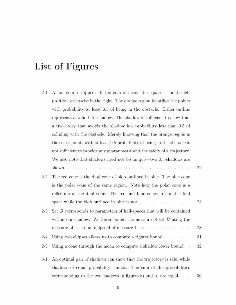
2-1 A fair coin is flipped. If the coin is heads the square is in the left
position, otherwise in the right. The orange region identifies the points
with probability at least 0.5 of being in the obstacle. Either outline
represents a valid 0.5−shadow. The shadow is sufficient to show that
a trajectory that avoids the shadow has probability less than 0.5 of
colliding with the obstacle. Merely knowing that the orange region is
the set of points with at least 0.5 probability of being in the obstacle is
not sufficient to provide any guarantees about the safety of a trajectory.
We also note that shadows need not be unique—two 0.5-shadows are
shown. . . . . . . . . . . . . . . . . . . . . . . . . . . . . . . . . . . . 22
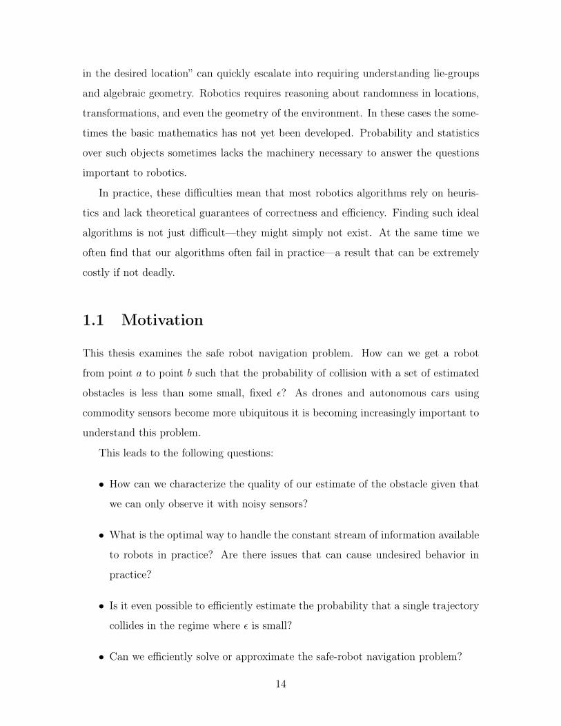
2-2 The red cone is the dual cone of blob outlined in blue. The blue cone
is the polar cone of the same region. Note how the polar cone is a
reflection of the dual cone. The red and blue cones are in the dual
space while the blob outlined in blue is not. . . . . . . . . . . . . . . 24
2-3 Set 𝐵 corresponds to parameters of half-spaces that will be contained
within our shadow. We lower bound the measure of set 𝐵 using the
measure of set 𝐴, an ellipsoid of measure 1− 𝜖. . . . . . . . . . . . . 28
2-4 Using two ellipses allows us to compute a tighter bound . . . . . . . . 31
2-5 Using a cone through the mean to compute a shadow lower bound. . 32
3-1 An optimal pair of shadows can show that the trajectory is safe, while
shadows of equal probability cannot. The sum of the probabilities
corresponding to the two shadows in figures a) and b) are equal. . . . 36
9

3-2 An visualization of the execution of algorithm 1 . . . . . . . . . . . . 39
4-1 Safe RRT . . . . . . . . . . . . . . . . . . . . . . . . . . . . . . . . . 45
4-2 An example of a variable gadget . . . . . . . . . . . . . . . . . . . . . 49
5-1 An illustration about how a robot can be always taking an action that
is safe, but still be guaranteed to eventually collide. . . . . . . . . . . 53
5-2 A flow chart for a policy that can cheat a natural definition of safety
using internal randomness . . . . . . . . . . . . . . . . . . . . . . . . 55
A-1 The dual cone of the blue blob . . . . . . . . . . . . . . . . . . . . . . 67
A-2 The polar cone of the blue blob. Note it’s relation with the dual cone. 68
10

List of definitions
1 Definition (𝜖−shadow) . . . . . . . . . . . . . . . . . . . . . . . . . . 21
2 Definition (Maximal 𝜖-shadow) . . . . . . . . . . . . . . . . . . . . . . 25
3 Definition (policy) . . . . . . . . . . . . . . . . . . . . . . . . . . . . 54
4 Definition (Policy Safety) . . . . . . . . . . . . . . . . . . . . . . . . . 54
5 Definition (Absolute Safety) . . . . . . . . . . . . . . . . . . . . . . . 55
6 Definition (Information Adversary) . . . . . . . . . . . . . . . . . . . 56
7 Definition (Convex Cone) . . . . . . . . . . . . . . . . . . . . . . . . 66
8 Definition (Dual Cone (𝐶⋆)) . . . . . . . . . . . . . . . . . . . . . . . 66
9 Definition (Polar Cone (𝐶0)) . . . . . . . . . . . . . . . . . . . . . . . 66
10 Definition (Norm Cone) . . . . . . . . . . . . . . . . . . . . . . . . . 66
11 Definition (Dual Norm (|| · ||⋆)) . . . . . . . . . . . . . . . . . . . . . 69
11

12

Chapter 1
Introduction
The writing of this thesis coincides with the rapid deployment of robots outside of
factories. Drones are inexpensive and widely available, basic autonomy is present in
mass-produced cars such as the Tesla Model S and robots are autonomously delivering
room service in high-end hotels.
Deploying a robot that operates robustly in unstructured environments remains
incredibly difficult. Rarely is it sufficient open a textbook, implement an algorithm
and release your robot into the wild. One contributing factor is the lack of efficient,
provably-correct algorithms that work on realistic models. For much of the state of
the art work, we expect it to fail in certain circumstances.
Many problems in robotics are provably hard to compute efficiently. Figuring
out how to move a robot between two configurations and several other variants of
planning problems are PSpace and NP-hard [23, 5, 28]. Figuring out where a robot
is in a map and other variants of the localization problem have also been shown to
be NP-Hard [6, 33]. Common variants of decision making under uncertainty are also
provably hard [17, 20]. While the dream of provably correct, efficient algorithms for
robotics would make life much easier for engineers, it’s not clear that it is achievable.
If all problems in robotics are robustly, provably hard, it doesn’t make sense to search
for such algorithms.
Robotics is also very difficult from a mathematical perspective. Even reasoning
about seemingly simple questions such as "what joint angles place the robot hand
13
in the desired location” can quickly escalate into requiring understanding lie-groups
and algebraic geometry. Robotics requires reasoning about randomness in locations,
transformations, and even the geometry of the environment. In these cases the some-
times the basic mathematics has not yet been developed. Probability and statistics
over such objects sometimes lacks the machinery necessary to answer the questions
important to robotics.
In practice, these difficulties mean that most robotics algorithms rely on heuris-
tics and lack theoretical guarantees of correctness and efficiency. Finding such ideal
algorithms is not just difficult—they might simply not exist. At the same time we
often find that our algorithms often fail in practice—a result that can be extremely
costly if not deadly.
1.1 Motivation
This thesis examines the safe robot navigation problem. How can we get a robot
from point 𝑎 to point 𝑏 such that the probability of collision with a set of estimated
obstacles is less than some small, fixed 𝜖? As drones and autonomous cars using
commodity sensors become more ubiquitous it is becoming increasingly important to
understand this problem.
This leads to the following questions:
∙ How can we characterize the quality of our estimate of the obstacle given that
we can only observe it with noisy sensors?
∙ What is the optimal way to handle the constant stream of information available
to robots in practice? Are there issues that can cause undesired behavior in
practice?
∙ Is it even possible to efficiently estimate the probability that a single trajectory
collides in the regime where 𝜖 is small?
∙ Can we efficiently solve or approximate the safe-robot navigation problem?
14

This thesis aims to address these questions through the development of both ef-
ficient algorithms and the mathematics necessary to understand the problem. While
this thesis is primarily focused on theoretical developments, it aims to understand is-
sues that the author encountered during more applied work in industry and academia.
1.2 Related Work
Robot navigation with uncertainty is a problem that has been studied in several
different contexts. The work can be divided into several categories: methods that
reason about planning under uncertainty in general fashion and are able to handle
safe robot navigation; methods that reasons about uncertainty in the state of the
robot; and methods that reason about uncertainty of the environment. There are
also two general classes of approaches to reasoning about uncertainty. The first class
of methods rely on Monte-Carlo based sampling techniques while others reason about
uncertainty in a more symbolic fashion.
One general model of reasoning about uncertainty is the Partially Observable
Markov Decision Process (POMDP) model—a markov decision process where the
state cannot always be directly observed [13]. POMDPs can model many robotics
problems with uncertainty including navigation, grasping and exploration [13, 9, 27].
Solving POMDPs is provably hard, and in some cases even undecidable [20, 17].
Though solving POMDPs is also often hard in practice, there is a large body of work
aiming to solve sufficiently small, structured POMDPs [15, 26, 21, 1, 31].
In practice it is often desirable to trade generality for performance and use an al-
gorithm tailored towards reasoning about uncertainty in robot navigation. The first
class of specialized methods focuses on uncertainty in the robot’s position and orien-
tation (pose) and how well the system tracks the desired trajectory. Some methods
attempt to quantify the uncertainty to identify how far the robot might stray from
the ideal trajectory. They then proceed to use that information to know how far away
to stay from obstacles [16, 4]. When the robot of interest has complicated, nonlin-
ear dynamics, robust motion plans can by computed using sum-of-square funnels for
15

characterizing how well a robot can recover from deviations from the ideal trajectory
[32, 18, 29, 30].
Other branches of work focus more on uncertainty in the shape and location of the
obstacles themselves. Some works attempt to identify shadows, or regions where the
obstacle could be and avoid those during planning [12, 24]. However, since models of
random geometry were not widely available and understood, these works often failed
to provide theoretical guarantees and sometimes make errors in their derivations
resulting in trajectories that are consistently unsafe [24]. Given a generative model
for obstacles, it becomes possible to develop a sampling-based method that is provably
safe [25, 11]. However, these methods have a runtime that depends on 1𝜖
where 𝜖 is
the allowable probability of collision. In the regime where the acceptable probability
of collision, 𝜖, is very small, these methods can become very slow.
1.3 Contributions and Outline
This thesis builds machinery to help understand and solve the safe navigation prob-
lem. Chapter 2 builds the mathematical foundations necessary to both understand
and solve the safe planning problem. It starts by addressing the question of how to
define a probability of collision. It defines a distribution over shapes which we use as
a model for the remainder of the work. Such obstacles are referred to as polytopes
with Gaussian distributed faces (PGDF). It then discusses how to compute the in-
tersection of probability of an arbitrary shape a random half-space drawn from any
distribution. It introduces the notion of a shadow—the generalization of a confidence
interval to shapes. The notion of shadows will be crucial in the development of ef-
ficient algorithms later in the work. Finally we show how to construct shadows for
the distribution defined earlier in the chapter. We believe this work has applications
beyond the safe navigation problem.
Chapter 3 discusses an efficient algorithm for bounding the probability of collision
of a trajectory. It develops an algorithm that can be used to bound the probability
of intersection of any collision checkable set with a set of PGDF obstacles. This
16

algorithm can be used to efficiently bound the probability that a robot trajectory will
collide with a set of estimated obstacles. While the probabilities produced by the
algorithm are not tight we briefly discuss tightness in the low-probability regime.
Chapter 4 discusses algorithms for the safe planning problem. It defines the safe
planning problem as the search for a robot trajectory with probability of collision
less than a fixed 𝜖. Then we examine the approximate safe planning problem where
the true probabilities of collision are replaced with the bounds computed using the
algorithm in chapter 3. We examine the computational complexity of the problem.
First we show a trivial, exponential time algorithm that shows the problem is in 𝑁𝑃 .
We then discuss the submodularity of the cost function which we hope can be used to
find a polynomial time algorithm to solve this approximate safe planning problem. We
briefly discuss some hardness results of the problem with high dimensional obstacles.
Chapter 5 examines the issues with generalizing the above methods to the online
setting where the robot has a constant stream of information and can change its
desired trajectory. This is the "safe” analog of transitioning from motion planning
to policy search. Unlike the setting where we are presented a single information set
before execution, safety is not guaranteed by always following a trajectory with a low
probability of collision. We present a toy example that illustrates this phenomenon.
Even though the robot is always following a safe trajectory, its probability of colliding
approaches 1. We suggest a different criterion for safety—guaranteeing that the
lifetime probability of collision does not exceed a particular value. We then present a
simple way of ensuring that such a criterion is met. We analyze when the presented
criterion is necessary in addition to sufficient. In order to better understand the
criterion we compare it to safety under an information oracle—an oracle which can cut
off the flow of information at any point in time. This helps us develop an equivalent,
more intuitive way to guarantee safety without relying on a mathematically technical
formulation. Finally we show how the algorithm introduced in chapter 3 can be
modified to ensure that a policy is safe.
Finally chapter 6 discusses future directions based on the presented work. We
discuss other potential applications of bounding random geometry, like manipulation
17

under uncertainty. We also discuss the development of better models and how they
can be understood using the machinery developed in chapter 2. We discuss directions
for future work on safe planning that are guided by the included complexity results
and known structure. Finally we take a step back and analyze the potential impact
of the presented ideas to the deployment of safe, efficient and reliable robots in the
real world.
18
Chapter 2
Shadows
In order to be able to provide safety guarantees for robot operation in domains with
uncertainty about obstacles, we must develop a formal understanding of the relation-
ship between randomness in the observations and resulting estimate. Consider the
following scenario: the robot must avoid an obstacle but gets only a noisy observation
of said obstacle. Given this noisy observation, it computes an estimate of the space
occupied by the obstacle and avoids this region. Given the observation, however, the
true space occupied by the obstacle is random and not guaranteed to be inside the
estimated region. It is not sufficient for the robot to avoid the estimated region to
ensure non-collision.
In order to provide theoretical guarantees about a robot’s operation in such a
domain we must develop mathematics regarding the random shapes that come from
estimating geometry with noisy observations. The ultimate aim of this chapter is to
develop shadows, a geometric equivalent of confidence intervals for uncertain obsta-
cles. The concept of shadows will prove useful in the development of provably correct
algorithms for safe robot navigation problem later in the thesis.
Understanding the mathematics behind shadows turns out to be rather involved.
Section 2.1 begins by formally defining the notion of an 𝜖-shadow. A significant
portion of the section is spent motivating our definition of shadows and seeing how it
avoids issues with previous methods of bounding random geometry. We then provide
an example of a distribution from which these random shapes can be drawn. We
19

introduce polytopes with Gaussian distributed faces (PGDF) which will be used to
develop examples and algorithms throughout this thesis.
It turns out that shadows can have surprising and non-intuitive behavior. In order
to build an intuition for shadows we provide some theorems that characterize half-
space shadows of any distributions. First we show how to find collision probabilities
between a random half-space and an any set. This helps introduce some of the basic
geometric notions that will be used to understand and construct shadows. We then
develop a theorem that helps us understand the existence and uniqueness of an 𝜖-
shadow for any distribution and a fixed 𝜖. The answers here are can be surprising
and suggest that random geometry can behave quite differently than random vectors.
Section 2.2 addresses the algorithmic question of how to compute shadows for
PGDF obstacles. It provides several algorithms for computing shadow lower bounds
for PGDF obstacles. Unlike the shadows of section 2.1, these bounds are often loose:
there are situations in which the computed 𝜖−shadow is also a 𝜖′−shadow for 𝜖′ < 𝜖.
We compare the tightness of these different shadow bounds in different scenarios.
We also present a general method of building 𝜖-shadows for polytopes given only a
mechanism for generating shadows of half-spaces, and we comment on the tightness
of the bounds generated with the method.
2.1 Mathematics of Shadows
In this section we develop the mathematical machinery necessary to build and char-
acterize shadows. Computational and algorithmic developments will be presented in
a later section.
2.1.1 Definitions
In this section we define the notion of a shadow as well as give an example distribution
of obstacles for which we can compute shadows for concrete obstacle estimates.
In order to be able to distinguish the space that the robot operates in from the
space of half-space parameters we introduce the following notation: bold, nonscript
20

capital letters refer to subsets of R𝑛 corresponding to the robot’s workspace. Our
robots usually operate in 𝑋 = R𝑛. 𝑋 refers to this vector space throughout the
document. Capital script letters refer to subsets of the dual of the robot’s workspace’
i.e., sets of half-space parameters over the robot’s workspace. Half-space obstacles can
be represented as points in 𝒳 = R𝑛. 𝒳 refers to this space of half-space parameters
throughout the document. We also note that the goal of the chapter is to bound
random obstacles. A random obstacle is defined as a random convex polytope which
the robot is not allowed to collide with. This analysis can be made applicable
Shadows
Definition 1 (𝜖−shadow). A set 𝑆 ⊆𝑋 is an 𝜖−shadow of a random obstacle 𝑂 if
𝑃 (𝑂 ⊆ 𝑆) ≥ 1− 𝜖.
It is important to note that an 𝜖−shadow may be quite different than the set of
points with probability more than 𝜖 of being inside the random obstacle as used by
Sadigh and Kapoor [24].
Guaranteeing non-intersection of the robot trajectory with the obstacle given only
the set of points of low probability of colliding, requires either understanding the
correlation between the event that nearby points collide or using a union bound over
all points in the trajectory.
Since robot trajectories necessarily pass through an infinite number of points, a
union-bound alone cannot be used to guarantee safety. While in this case, a guarantee
can be found using smoothness of the Gaussian PDF and constructing simplices that
enclose the trajectory, doing so introduces additional restrictions on the resulting
trajectories. In practice this usually causes the the computed probability bound to
be greater than 1, rendering the theoretical guarantees of the algorithm useless.
An example of the difference between a shadow and the set of points likely in the
obstacle can be see in figure 2-1. The shadow is a subset of the likely points, but can
used to verify the trajectory of the safety. The set of likely points is not sufficient
information to verify the safety of the trajectory.
21

Figure 2-1: A fair coin is flipped. If the coin is heads the square is in the left position,otherwise in the right. The orange region identifies the points with probability atleast 0.5 of being in the obstacle. Either outline represents a valid 0.5−shadow. Theshadow is sufficient to show that a trajectory that avoids the shadow has probabilityless than 0.5 of colliding with the obstacle. Merely knowing that the orange region isthe set of points with at least 0.5 probability of being in the obstacle is not sufficientto provide any guarantees about the safety of a trajectory. We also note that shadowsneed not be unique—two 0.5-shadows are shown.
Polytopes with Gaussian Distributed Faces
Computing shadows requires having some sort of characterization of the uncertainty
with respect to obstacles in the environment. We formalize this notion as assumptions
about the distribution from which obstacles are drawn.
We use homogeneous coordinates throughout for simplicity. We recall that a
polytope 𝑃 ⊆𝑋 is the intersection of half-spaces:
𝑃 =⋂︁𝑖
𝛼𝑇𝑖 𝑥 ≤ 0.
We consider the case where the parameters 𝛼1...𝑘 are drawn from Gaussian distri-
butions with known parameters. From here on, a polytope with parameters drawn
from Gaussian distributions is referred to as a polytope with Gaussian distributed
faces (PGDF). Note that for any 𝜆 ≥ 0, 𝜆𝛼 and 𝛼 correspond to the same half-space.
We will show that this model can be derived under reasonable conditions and discuss
the fundamental limitations and drawbacks of the model.
This model is relevant because it can be derived from segmented point-cloud data.
If we are given a point cloud representation of the obstacle with points grouped by face
and the points are observed with Gaussian noise then the true faces can be estimated
with a linear regression. If this regression is performed in a Bayesian setting, the
22

posterior distribution over the face parameters is a Gaussian distribution, suggesting
that assuming 𝛼 is Gaussian distributed is reasonable [2, 22].
The model, however, does discard information often available to robotic systems.
Robot sensors such as Kinects and LIDARs often provide point clouds in conjunction
with free space information. In addition to identifying the first time each “ray" hits
an obstacle in the environment, these sensors also provide the information that the
space in between the sensors and the point is likely collision free.
Later in this chapter we show how to efficiently compute 𝜖−shadows for the PGDF
model in practice.
2.1.2 A characterization of half-space Shadows
Before we discuss how to compute shadows efficiently in practice, we develop a math-
ematical theory of shadows to help get intuition for their behavior. For random
half-spaces of any distribution we will answer the following questions: When does
there exist an 𝜖-shadow? Are shadows unique?
We connect the notion of a shadow with the classic notions of dual and polar cones
in convex analysis. The analysis in this section is done with complete generality and
does not assume that obstacles are PGDF. The only restriction, which we take to make
analysis cleaner, is that sets with an empty interior under the standard topology have
zero measure. More intuitively, we assume the probability that we select parameters
from a zero volume set is zero.
Exact Probabilities of Intersection
First we compute the exact probability that a random half-space 𝛼𝑇𝑥 ≤ 0, parametrized
by 𝛼, will intersect an arbitrary set 𝐴 ⊆𝑋. We relate this value to the measure of a
dual cone, a notion from convex geometry. More formally, we examine how to find:
𝑃 (∃𝑥 ∈ 𝐴 such that 𝛼𝑇𝑥 ≤ 0).
Theorem 1. 𝑃 (∃ 𝑥 ∈ 𝐴 : 𝛼𝑇𝑥 ≤ 0) = 1− 𝜇(𝒞⋆) where 𝒞⋆ is the dual cone of 𝐴.
23
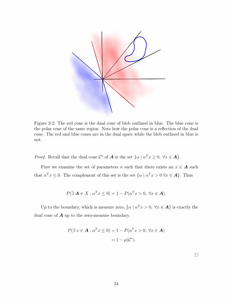
Figure 2-2: The red cone is the dual cone of blob outlined in blue. The blue cone isthe polar cone of the same region. Note how the polar cone is a reflection of the dualcone. The red and blue cones are in the dual space while the blob outlined in blue isnot.
Proof. Recall that the dual cone 𝒞⋆ of 𝐴 is the set {𝛼 | 𝛼𝑇𝑥 ≥ 0, ∀𝑥 ∈ 𝐴}.
First we examine the set of parameters 𝛼 such that there exists an 𝑥 ∈ 𝐴 such
that 𝛼𝑇𝑥 ≤ 0. The complement of this set is the set {𝛼 | 𝛼𝑇𝑥 > 0 ∀𝑥 ∈ 𝐴}. Thus
𝑃 (∃ 𝐴 ∈ 𝑋 : 𝛼𝑇𝑥 ≤ 0) = 1− 𝑃 (𝛼𝑇𝑥 > 0, ∀𝑥 ∈ 𝐴).
Up to the boundary, which is measure zero, {𝛼 | 𝛼𝑇𝑥 > 0, ∀𝑥 ∈ 𝐴} is exactly the
dual cone of 𝐴 up to the zero-measure boundary.
𝑃 (∃ 𝑥 ∈ 𝐴 : 𝛼𝑇𝑥 ≤ 0) = 1− 𝑃 (𝛼𝑇𝑥 > 0, ∀𝑥 ∈ 𝐴)
= 1− 𝜇(𝒞*).
24
Shadows and Polar Cones
A related notion in convex geometry, the polar cone, allows us to relate the con-
struction of shadows with a distribution in the halfspace parameter space. Please see
appendix A for the related definitions. A correspondence theorem defines a bijection
between a set we understand (polar cones) and a set we are trying to characterize
(shadows). This will allow use to use our knowledge of the existence and uniqueness
of polar cones to understand the existence and uniqueness of shadows.
The proof of the correspondence theorem (theorem 3) will highlight a problem
with our current definitions. Since a 0.25−shadow is also a 0.5−shadow, it will prove
difficult to construct a one-to-one map between all shadows and another object which
we understand. Thus we consider only maximal shadows.
Definition 2 (Maximal 𝜖-shadow). An 𝜖−shadow 𝐴 ⊆ 𝑋 of a random shape 𝑂 is
maximal if 𝑃 (𝑂 ⊆ 𝐴) = 1− 𝜖.
This leads to our first, and most general, method of constructing shadows.
Theorem 2. For every set 𝒴 ⊆ 𝒳 of measure 1 − 𝜖, the polar cone 𝒞0 of 𝒴 is a
𝜖−shadow for the random shape defined by the measure.
Proof. Recall that a point 𝑥 is in collision with the halfspace defined by 𝛼 if 𝛼𝑇𝑥 ≤ 0.
Consider a set 𝒴 of measure 1 − 𝜖. Since sets with empty interiors have zero
measure, we can assume without loss of generality that 𝒴 is open.
First we identify the set of points 𝐴 = {𝑥 | 𝛼𝑇𝑥 > 0, ∀𝛼 ∈ 𝒴} ⊆ 𝑋, that is the
set of points not inside any halfspace defined by a point in 𝒴 . Up to the boundary,
which is a set of measure zero, this is exactly the polar cone, 𝐶0 of 𝒴 .
With probability 1 − 𝜖, a draw of 𝛼 will be in 𝒴 and thus not correspond to a
halfspace that intersects 𝐶0. This implies that 𝐶0 is an 𝜖−shadow.
Theorems 1 and 2 can be combined to give a correspondence theorem that will
allow us to better understand shadows.
Theorem 3. There is a one-to-one correspondence between convex cones in parameter
space of measures 1− 𝜖 and maximal 𝜖-shadows.
25

Proof. Our proof will show that applying the construction in theorems 1 and 2 and
reversed yields the identity.
First we start with a convex cone in the space of half-space parameters, 𝒴 , of
measure 1 − 𝜖. Theorem 2 tells us that the polar cone of 𝒴 is an 𝜖−shadow. The
construction in theorem 1 tells us that the probability of the shadow not containing
the random halfspace is the measure of the negative of it’s dual cone.
Since 𝒴 is a convex cone, the negative of the dual cone of the polar cone the
original set 𝒴 itself.
The same procedure works for the reverse direction.
Theorem 3 gives us guidelines about how to construct shadows. It shows that the
sets used to compute the probabilities of shadows should be convex cones if we wish
for our shadows to be tight.
It also gives insight to when to when 𝜖−shadows are not unique. Any set of
measure 1− 𝜖 with a distinct polar cone can be used to create a distinct shadow.
The non-uniqueness gives insight into why not all shadows are equivalent when
bounding the probability of intersection. One 𝜖−shadow may be sufficient to certify
non-collision, but another might not. This suggests that we will have to search
through a continuous set of shadows for the one that gives the strongest bound.
Finally it helps us answer the question of whether nontrivial shadows always exist.
In 𝒳 = R𝑛, if the distribution over parameters is such that any halfspace through
the origin has measure greater than 𝜖 then the only shadow is the entire space (the
trivial shadow). This comes from the fact that the minimal convex cone with suf-
ficient measure then becomes the entire space. For example, consider constructing
an 𝜖 = 0.25-shadow with 𝛼 ∼ 𝒩 (0, 𝐼). The distribution is symmetric and all halfs-
paces through the origin have measure 0.5. Thus we cannot construct any non-trivial
0.25−shadows for this distribution.
This suggests a procedure by which we can find the maximal 𝜖 such that no 𝜖-
shadow smaller than the full space cannot exist.
26

Theorem 4. Let
𝜖⋆ = inf𝛼∈𝒳
𝜇(𝛼𝑇𝑥 ≤ 0)
Then for all 𝜖′ < 𝜖, there do not exist any 𝜖′−shadows.
Since any convex cone that strictly contains a halfspace through the origin must be
the entire vector space, and no halfspace has measure more than 𝜖, for any 𝛿 < 𝜖 there
cannot exist an 𝛿−shadow. In other words there is no shadow that contains the set
with probability more than 1−𝜖. We note that for PGDF obstacles there always exists
an 𝜖 ∈ (0, 1) such that a non-trivial shadow does not exist. This fact is surprising,
does not match our intuition and suggests that care must be taken in ensuring that
planning methods are truly safe. Future work also includes understanding whether
other important models of random geometry also undergo this phase transition.
2.2 Computing Shadows for PGDFs
In the previous section we constructed shadows for halfspace obstacles in full gen-
erality. Unfortunately, even the integrals required to determine the probability that
a shadow contains an obstacle can be difficult to compute. In this section we will
suggest three different ways to compute shadow lower bounds. Instead of trying to
compute a shadow that is tight with respect to its probability, we will construct shad-
ows for which it is easy to compute a lower bound on the probability that a shadow
contains a random shape. At first we will restrict our attention to halfspaces from
a PGDF faces. In section 2.2.3 we will use the developments in the previous section
to construct a shadow for a PGDF with an arbitrary number of faces. Sections 2.2.1
and 2.2.1 present bounds that are more effective when the parameters of the half-
space are relatively well known (when the mean of the distribution is far from the
origin with respect to the norm induced by the precision matrix) and section 2.2.2
presents a bound that works better when there is relatively little information about
the parameters.
27

2.2.1 Gaussian Elliptical Shadows
Figure 2-3: Set 𝐵 corresponds to parameters of half-spaces that will be containedwithin our shadow. We lower bound the measure of set 𝐵 using the measure of set𝐴, an ellipsoid of measure 1− 𝜖.
In this section we construct a shadow for a given distribution of random shapes
as follows. We identify a sufficiently large scaled covariance ellipse around the mean
parameter vector such that its measure is 1− 𝜖. We then take the polar cone of this
ellipse and use it as our shadow. A pictorial outline of the derivation is presented in
figure 2-3.
We begin by identifying required size of the covariance ellipse.
Lemma 1. Let 𝛼 ∼ 𝒩 (𝜇,Σ), 𝜑 be cdf of the Chi-Squared distribution with 𝑛 degrees
of freedom and:
𝒳 = {𝛽 | (𝛽 − 𝜇)𝑇Σ−1(𝛽 − 𝜇) ≤ 𝜑−1(1− 𝜖))}.
Then 𝑃 (𝛼 ∈ 𝑋) = 1− 𝜖.
Proof. First we note that 𝛼 is equal in distribution to Σ𝛼′+𝜇 with 𝛼′ ∼ 𝒩 (0, 𝐼). 𝛼′𝑇𝛼′
is then a Chi-Squared random variable with 𝑛 degrees of freedom. Thus 𝑃 (𝛼′𝑇𝛼′ ≤
𝜑−1(1− 𝜖)) = 1− 𝜖. If we let 𝑍 = {𝛼 | 𝛼𝑇𝛼 ≤ 𝜑−1/2(1− 𝜖)} then 𝑃 (𝛼′ ∈ 𝑍) = 1− 𝜖.
Let 𝑌 be the image of 𝑍 under the map we used to generate a random variable
28

identical in distribution to 𝛼. Then 𝑌 = {𝛽 | (𝛽 − 𝜇)𝑇Σ−1(𝛽 − 𝜇) ≤ 𝜑−1(1− 𝜖)} and
the measure of 𝑌 under the distribution over 𝛼 must be the same as the measure of
𝑍 under the distribution over 𝛼′. Thus 𝑃 (𝛼 ∈ 𝑌 ) = 1− 𝜖.
Now, given this ellipse of sufficient measure, we can compute its polar cone and
resulting 𝜖−shadow. We note that if the ellipse given in lemma 1 contains the origin
in its interior, the resulting polar cone will be empty. We compute the polar cone by
first computing the minimal cone 𝒞 which contains the ellipse, and then computing
the polar cone of 𝒞.
For the remainder of the section we assume that the space has been rotated and
scaled such that 𝜇 = (0..., 0, 1).
Theorem 5. For nondegenerate PGDF halfspaces, there exists Σ′ such that
𝑋 = {< 𝑥1....𝑥𝑛−1, 𝑧 >| 𝑥𝑇Σ𝑥 ≥ 𝑧}
is an 𝜖−shadow.
Our proof is constructive and tells us how to compute Σ.
Proof. Let 𝒳 = {𝛽 | (𝛽 − 𝜇)𝑇Σ(𝛽 − 𝜇) ≤ 𝑟2} be the ellipse identified in lemma 1.
We expand the equation of the above surface for convenience:
𝑟2 = (𝛽 − 𝜇)𝑇Σ(𝛽 − 𝜇)
= 𝛽𝑇Σ𝛽 − 2𝛽𝑇Σ𝜇 + 𝜇𝑇Σ𝜇.
Now we compute the equation for the normals to the surface at point 𝑥
2Σ𝑥− 2Σ𝜇.
Then we identify the set where the normal vectors are orthogonal to the vector to the
29
point 𝑥:
𝑥𝑇 (Σ𝑥− Σ𝜇) = 0
𝑥𝑇Σ𝑥− 𝑥𝑇Σ𝜇 = 0
𝑥𝑇Σ𝑥 = 𝑥𝑇Σ𝜇.
Plugging this into the equation of the original ellipse gives us the equation for the
plane that contains the set where the ellipse is tangent to the minimal containing
cone:
𝛽𝑇Σ𝜇− 2𝛽𝑇Σ𝜇 + 𝜇𝑇Σ𝜇 = 𝑟2
−𝛽𝑇Σ𝜇 + 𝜇𝑇Σ𝜇 = 𝑟2
𝜇𝑇Σ𝛽 = 𝜇𝑇Σ𝜇− 𝑟2.
This is a linear equation in 𝛽 which we can use this to solve for 𝛽𝑛 in terms of the
remaining indices of 𝛽. Substituting it plugged into the original equation yields the
equation of a new ellipse. Let Σ𝐸, 𝑥0, 𝑟′ be the parameters of this new ellipse in the
form (𝛽𝑇1...𝑛−1 − 𝑥0)
𝑇Σ𝐸(𝛽1...𝑛−1 − 𝑥0) ≤ 𝑟′2.
Now we can directly identify the equation of the cone as:
𝛽𝑇
⎛⎝Σ𝐸 0
0 −𝑟2
⎞⎠ 𝛽 ≤ 0; 𝛼𝑛 ≥ 0.
Alternatively we can describe the set as {𝛽 |√︁𝛽𝑇1..𝑛−1Σ
′𝛽1..𝑛−1 ≤ 𝛽𝑛}, where Σ′ = Σ𝐸
𝑟2.
This identifies our cone as a standard-norm cone with the norm induced by Σ′, and
makes finding the dual cone a standard problem. The dual cone is just ||𝛽1...𝑛||⋆ ≤ 𝛽𝑛
where || · ||⋆ denotes the dual norm [see 3, example 2.25, page 52]. The dual norm is
the natural one induced by Σ′−1. Thus the dual cone is
𝛽𝑇
⎛⎝Σ′−1 0
0 1
⎞⎠ 𝛽 ≤ 0; 𝛽𝑛 ≥ 0.
30
Finally since 𝐶0 = −𝐶⋆ we can write down the equation of the polar cone which
defines the shadow.
𝛽𝑇
⎛⎝Σ′−1 0
0 1
⎞⎠ 𝛽 ≤ 0; 𝛽𝑛 ≤ 0
When we dehomogenize the coordinate system we get a conic section as a shadow.
We refer to Handlin’s Conic Sections Beyond R2 for a classification of different sections
and a discussion of conic sections in high dimensions [8], but we note that this step
implies that the procedure does not always produce non-degenerate shadows.
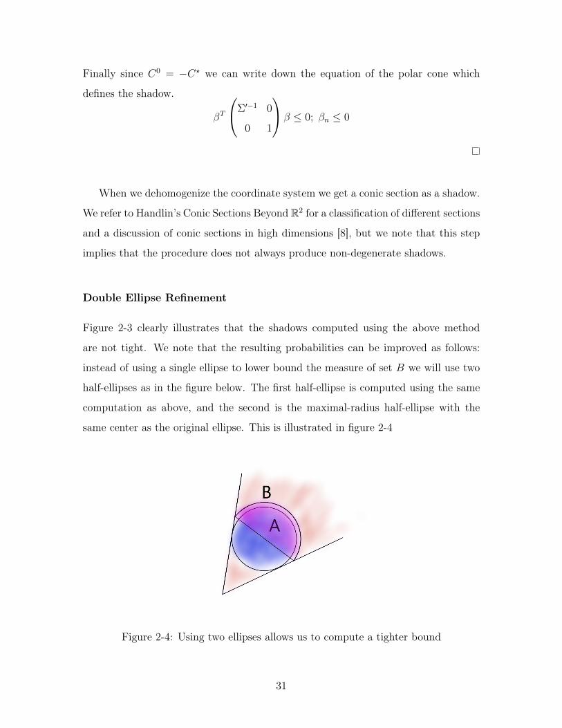
Double Ellipse Refinement
Figure 2-3 clearly illustrates that the shadows computed using the above method
are not tight. We note that the resulting probabilities can be improved as follows:
instead of using a single ellipse to lower bound the measure of set 𝐵 we will use two
half-ellipses as in the figure below. The first half-ellipse is computed using the same
computation as above, and the second is the maximal-radius half-ellipse with the
same center as the original ellipse. This is illustrated in figure 2-4
Figure 2-4: Using two ellipses allows us to compute a tighter bound
31

2.2.2 Conic Shadows
We note that the shadow bounds derived in section 2.2.1 fail to provide a non-trivial
shadow when the covariance is too “small” relative to the distance of the mean from
the origin. As this becomes the case another class of shadow lower bound approaches
being tight. We suggest how such a bound can be computed below. We can compute
the measure of a cone going through the mean of the distribution by transforming
our space to one where the Gaussian distribution is Isotropic and then computing the
portion of the full space taken up by cone. This process is illustrated in figure 2-5.
Figure 2-5: Using a cone through the mean to compute a shadow lower bound.
2.2.3 From Halfspaces to Polytopes
The previous sections focused on half-spaces because duality is very intimately re-
lated to the construction of shadows. This relationship is not as powerful for general
polytopes, and makes computing the exact probabilities corresponding to shadows
difficult without a large enumeration.
Recall that a polytope is defined as the intersection of half-spaces⋂︀𝑖
𝛼𝑇𝑖 𝑥 ≤ 0.
Constructing tight shadows for polytopes in practice depends critically on understand
the correlation between 𝛼1...𝑛. In this section we make no assumptions regarding the
correlation between the 𝛼’s. In practice, we may have strong prior shape information
but a poor estimate of the location of the object. In this case our shadows would not
32
be maximal. In other words, there may exist a strictly smaller set that is also a valid
𝜖-shadow. We demonstrate an example where our shadows are tight, and provide
some analysis suggesting cases the shadows we construct are close to tight. Exploring
how knowledge of correlation may be used to produce tighter shadows for polytopes
remains an interesting direction for future work.
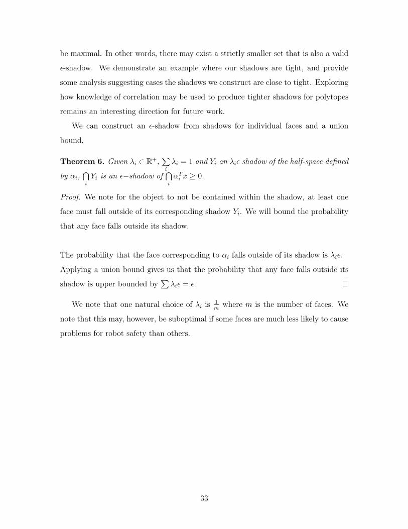
We can construct an 𝜖-shadow from shadows for individual faces and a union
bound.
Theorem 6. Given 𝜆𝑖 ∈ R+,∑︀𝑖
𝜆𝑖 = 1 and 𝑌𝑖 an 𝜆𝑖𝜖 shadow of the half-space defined
by 𝛼𝑖,⋂︀𝑖
𝑌𝑖 is an 𝜖−shadow of⋂︀𝑖
𝛼𝑇𝑖 𝑥 ≥ 0.
Proof. We note for the object to not be contained within the shadow, at least one
face must fall outside of its corresponding shadow 𝑌𝑖. We will bound the probability
that any face falls outside its shadow.
The probability that the face corresponding to 𝛼𝑖 falls outside of its shadow is 𝜆𝑖𝜖.
Applying a union bound gives us that the probability that any face falls outside its
shadow is upper bounded by∑︀
𝜆𝑖𝜖 = 𝜖.
We note that one natural choice of 𝜆𝑖 is 1𝑚
where 𝑚 is the number of faces. We
note that this may, however, be suboptimal if some faces are much less likely to cause
problems for robot safety than others.
33

34

Chapter 3
Algorithm for Bounding Probability
of Collision
In this section we focus on bounding the probability that a given robot trajectory
collides with a set of obstacles drawn from the posterior distribution of a Bayesian
estimation process. One of the most important consequences of the developments of
chapter 2 is a fast algorithm for bounding the probability that a fixed set intersects
a PGDF obstacle. We develop a generic algorithm that can bound the probability of
intersection between a set of PGDF obstacles with any collision-checkable set.
3.1 Motivation
One way to estimate the probability of collision is to use a Monte Carlo technique
based on sampling the location of obstacles and collision checking the trajectory. Take
for example the following naïve algorithm. Sample 𝑛 sets of obstacle geometries and
let 𝑝 be the portion of these geometries for which there is a collision. This algorithm
is very simple and does not introduce any slackness (𝐸[𝑝] is the exact probability
of collision). However, if you want to guarantee the probability of collision is less
than 𝜖, 𝑛 must be at least 𝑂(︀1𝜖
)︀samples for this method to be useful. In essence
the algorithm has to see at least a couple of failures in expectation to be useful.
This a fundamental limitation of sampling based algorithms that do not sample in a
35
transformed space.
In the context of robot safety, where we want robot collisions to be extremely rare
events (ex. 𝑝 = 10−7), this implies that Monte Carlo methods tend to perform poorly.
While variance reduction techniques have been shown to improve performance, it is
not sufficient in the regime where collisions happen rarely [10].
In this chapter we show how the 𝑂(︀1𝜖
)︀dependence can be avoided by searching
for shadows instead of sampling. We will search for a certificate, or proof, that the
probability is less than 𝜖. This will enable our method to have a complexity 𝑂(︀log 1
𝜖
)︀,
linear in the number of required digits of precision. Searching for a shadow also results
in tighter bounds than previous work without sacrificing correctness. Another benefit
of searching for shadows is that it avoids the slackness that would be introduced by
taking shadows of the same probability and using a union bound to compute the
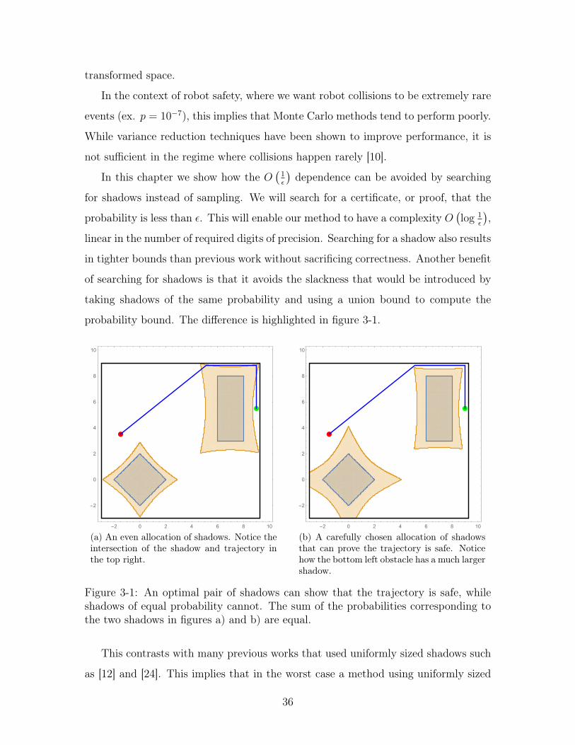
probability bound. The difference is highlighted in figure 3-1.
-2 0 2 4 6 8 10
-2
0
2
4
6
8
10
(a) An even allocation of shadows. Notice theintersection of the shadow and trajectory inthe top right.
-2 0 2 4 6 8 10
-2
0
2
4
6
8
10
(b) A carefully chosen allocation of shadowsthat can prove the trajectory is safe. Noticehow the bottom left obstacle has a much largershadow.
Figure 3-1: An optimal pair of shadows can show that the trajectory is safe, whileshadows of equal probability cannot. The sum of the probabilities corresponding tothe two shadows in figures a) and b) are equal.
This contrasts with many previous works that used uniformly sized shadows such
as [12] and [24]. This implies that in the worst case a method using uniformly sized
36
shadows can only find a plan if an 𝜖𝑛
safe plan exists. Not only can this lead to un-
necessarily conservative behavior, it also has a dependence on the environment that
does not necessarily affect the true probabilities of collision in a way that matches
our intuition. For safety what matters is the number of obstacles “close” (measured
by a combination of distance and uncertainty) to the trajectory, not just the number
of obstacles present in the environment. Searching for shadows instead of choosing
their size uniformly allows us to close the quality gap between geometric/symbolic
algorithms and Monte-Carlo algorithms by a factor of 𝑛, without sacrificing correct-
ness.
An interesting byproduct of our algorithm is a safety certificate. Our method finds
a set of shadows that show the trajectory in question is safe with probability at least
1− 𝜖. These shadows provide easy to verify, interpretable, proof that the trajectory is
safe. These certificates can be used to understand which obstacles are likely to collide
with the robot and which are not. Formally the problem we address is follows: given
a set 𝑋 and PGDF obstacles drawn from distributions with parameters 𝜇𝑖𝑗,Σ𝑖𝑗, find
the minimal 𝜖 such that the probability that an obstacle intersects 𝑋 is less than 𝜖.
We explain our algorithm in two parts. First, in section 3.2 we present an algorithm
that bounds the probability that a single obstacle intersects the fixed set. This allows
us to focus on the search of a single shadow and understand the restrictions of our
algorithm. In section 3.3 we present serial and parallel versions of the algorithm for
many obstacles and discuss computational complexity in further detail.
3.2 The Single Obstacle Case
In the case of a single obstacle, we can frame finding a probability bound as the search
for the maximal shadow. In other words we wish to find a solution to the following
optimization problem where 𝑋 is the set of states visited by the robot trajectory (the
37

swept volume):
minimize𝜖∈(0,1)
𝜖
subject to shadow(𝜖) ∩𝑋 = ∅(3.1)
It is not immediately clear that this optimization is convex, or otherwise solvable
in polynomial time. In order to make the optimization easily solvable we restrict
ourselves to a class of easily computable shadow lower bounds obtained in chapter
2. In particular, we restrict ourselves to shadows coming from the single and double
ellipse bounds for PGDF obstacles presented in sections 2.2.1 and 2.2.1 combined with
theorem 6. When this mapping is non-degenerate, it is a one-to-one from probabilities
to shadows. Let 𝑆(𝜖) be one of these two maps. We restrict ourselves to the following
optimization:
minimize𝜖∈(0,1)
𝜖
subject to S(𝜖) ∩𝑋 = ∅(3.2)
An important property of the map is that it is monotone. If 𝜖1 ≥ 𝜖2 then 𝑆(𝜖1) ⊂
𝑆(𝜖2). This implies that the set of probabilities that map to shadows that do not
intersect 𝑋 is an interval subset of (0, 1). This means that we can find the minimal
𝜖 for this class of shadows with a simple bisection search on the interval (0, 1). The
pseudocode for this search is presented in algorithm 1 and a figure illustrating the
execution is shown in figure 3-2.
To achieve precision 𝜖, algorithm 1 requires 𝑂(︀log 1
𝜖
)︀iterations due to the bisection
search. In every iteration there is a single call to a collision checker.
3.3 Generalization to Multiple Obstacles
In this section we generalize algorithm 1 to handle multiple obstacles, analyze the
resulting computational complexity, and show that it provides a tighter bound on the
probability of collision than previous work. We refer to the collision probability as
38

(a) First iteration of the bisection search (b) Second iteration of the bisectionsearch
(c) Third iteration of the bisectionsearch. Since it overshot in this iter-ation (detected as a collision betweenthe shadow and robot by the collisionchecker) it will try a smaller shadow inthe next iteration
(d) Fourth and final iteration of the bi-section search as it has found a shadowthat does not collide within the desirednumerical precision of the optimal one.
Figure 3-2: An visualization of the execution of algorithm 1
39

Algorithm 1 Finding an Optimal Shadow
1: function FindOptimalShadow(𝑋,𝜇,Σ, 𝜀)2: 𝜖𝑚𝑖𝑛 ← 03: 𝜖𝑚𝑎𝑥 ← 14: while 𝜖𝑚𝑎𝑥 − 𝜖𝑚𝑖𝑛 ≤ 𝜀 do5: 𝜖 ← 𝜖𝑚𝑎𝑥−𝜖𝑚𝑖𝑛
2
6: S ← GenerateShadow(𝜇,Σ, 𝜖)7: if Intersects(S,X) then8: 𝜖𝑚𝑖𝑛 ← 𝜖9: else
10: 𝜖𝑚𝑎𝑥 ← 𝜖11: end if12: end while13: return 𝜖𝑚𝑎𝑥
14: end function
risk throughout this section.
In order to generalize algorithm 1 we search for a separate shadow for each obstacle
and then sum up the probabilities for each shadow (justified by a union bound). The
search can be done for each obstacle in parallel.
Algorithm 2 Finds a bound on the risk of the set 𝑋 intersecting a set of randomobstacles.
1: function AggregateRiskBound(𝑋,𝜇1...𝑛,Σ1...𝑛, 𝜀)2: for 𝑖← 1...𝑛 do3: 𝜖𝑖 ← FindOptimalShadow(𝑋,𝜇𝑖,Σ𝑖,
𝜀𝑛)
4: end for5: return
∑︀𝑖
𝜖𝑖
6: end function
After compensating for the increased numerical precision necessary for multiple
obstacles, we get the computational complexities presented in table 3.1.
Table 3.1: Computational complexity of shadow finding in algorithm 2 for numericalprecision 𝜀, minimum probability 𝜖 and 𝑛 obstacles
serial parralelcollision checker calls 𝑂(𝑛 log 𝑛 log 1/𝜖) 𝑂(log 𝑛 log 1/𝜖)number of threads 1 𝑂(𝑛)
We note that the parallel algorithm is work-efficient—it does not do any more
40

work than the serial algorithm.
It is important to compare the complexity of the given algorithm compared to that
of a collision check with 𝑛 objects. Our algorithm is able to bound the probability
of collision with only a 𝑂(log 𝑛 log 1/𝜖) slowdown compared to a collision check with
obstacles of a known location. This suggests that robots can be made behave safely
and reason about uncertainty without greatly increasing the required computation.
3.4 Verification of Safety Certificates
We note that the low computational complexity of algorithm 2 implies that it can be
run on an embedded system with limited computational resources. This allows an
low power system to verify that actions suggested by another system, perhaps with
significantly more computational resources, is safe. It also allows us to verify that
the trajectories found by an algorithm dependent on heuristics or machine learning
is truly safe.
For systems that are even more computationally constrained we note that verifi-
cation is possible with a single collision check. If we stores the probabilities for the
individual shadows in algorithm 2, we can verify that a trajectory is safe with very
little communication and computational overhead. This would only require a single
collision check by the low-power system. In terms of communication, it requires only
the transmission of these probabilities, the states visited by the trajectory, and the
parameters of the obstacle distribution.
41

42

Chapter 4
Algorithms for Finding Safe Plans
In chapter 3 we demonstrated that the computational complexity of bounding the
probability of collision for a trajectory is asymptotically not not much more expensive
than a traditional deterministic collision check. It does not seem that a similar result
is possible for either minimum risk or risk constrained planning with the shadows
used in 3. In this chapter we present a NP-hardness result for the risk constrained
planning. In a sense our hard our NP-hardness result is unsatisfying as it requires
that the obstacles live in a space of dimension 𝑂(log 𝑛). In practice robots operate
in a space of dimension 3 which means this proof does not preclude the existence of
an efficient algorithm for safe planning. It does suggest that if an efficient algorithm
were to exist, it would have to use the properties of a space of fixed dimension. For
completeness, a naïve, exponential time algorithm is described in this chapter as well.
4.1 Motivation
While finding trajectories that can avoid obstacles with high probability has become
increasingly important, the safe motion planning problem lacks certain structures that
make the deterministic motion planning problem comparably easy to solve. This ends
up making it difficult to efficiently provide the same theoretical guarantees to safe
motion planning that are available in the deterministic setting.
One way of evaluating a deterministic motion planner is asking whether it is prob-
43
abilistically complete—does the probability of finding a plan, if one exists, approach 1
as the amount of allowed computation approaches infinity? While sampling based mo-
tion planning algorithms are often probabilistically complete under mild conditions,
they cannot be applied directly to the safe motion planning case without paying a
high computational cost.
Safe motion planning does not satisfy the Bellman principle of optimality. In other
words it lacks the important Markov-like Dynamic Programming structure that al-
lows sampling-based methods like the Rapidly-exploring Random Tree (RRT) family
of motion planning algorithms to be probabilistically complete. When evaluating
completeness for deterministic motion planning the trajectory used to reach a par-
ticular state, only that it is reachable. In the safe motion planning problem the
trajectory taken to reach a particular configuration is critical—it is exactly what de-
termines the probability of collision. Furthermore, since the probability of collision
at different points along a trajectory is not independent, the reachability of future
configurations under a risk constraint is dependent on the previous trajectory. Since
the RRT family of planners generally maintain only one path to every configuration
(thus the term random tree), they may not find the safe path if multiple feasible
paths exist. This suggests that simply adding a risk constraint to the standard RRT
algorithm is not probabilistically complete. An execution of an RRT to only generate
safe plans is shown in figure 4-1 to illustrate the issue.
This suggests that a different approach is necessary for approaching the safe mo-
tion planning problem. In approaching the safe motion planning problem, we propose
a naïve algorithm based on a Rapidly-exploring Random Graph (RRG) developed for
optimal deterministic motion planning [14]. This naïve algorithm will require expo-
nentially more computation than the original RRG algorithm. This algorithm will be
probabilistically complete under the standard assumptions for deterministic motion
planning. While the algorithm requires a lot of computation to find a safe plan once
that plan is present in the graph found by the RRG, it suggests that the method of
approximating paths in the robot’s configuration space can remain unchanged.
We will then show that finding a modification to the above algorithm that makes
44

(a) An execution of an RRT modified to only find safeplans. Uniformly sized shadows are shown for reference.
(b) The trajectory found by the RRT between thestart and destination configuration with optimal shad-ows found by algorithm 2. Note that the RRT tendsto choose suboptimal trajectories (this can be shown tohappen with probability 1). While this suboptimalitydoes not affect it’s ability to find trajectories in a deter-ministic setting, it does affect its ability to find trajecto-ries in a risk constrained setting since it cannot reducetotal risk “taken” to get to a particular configuration.
Figure 4-1: Safe RRT
45

it polynomial time is difficult. We provide several proof outlines for variants of the
hardness result. First we construct a reduction from 3SAT to the safe planning
problem where the obstacles are in a space of dimension 𝑂(𝑛). We then describe how
the result can be strengthened in several ways. We discuss how an Application of the
Johnson-Lindenstrauss lemma can allow us to use a space of dimension 𝑂(log 𝑛). We
also show how in the reduced space we can strengthen our result to prove hardness
of multiplicative approximation to a 1±Θ(︀1𝜖
)︀factor.
4.2 A Probabilistically Complete Planner for Safe
Motion Planning
In this section we propose a probabilistically complete safe planner. In other words, if
there exists a safe trajectory 𝜏 and a 𝛿 > 0 such that the 𝛿-inflation of the trajectory
{(𝑥, 𝑡) | 𝑑(𝑥, 𝜏(𝑡)) ≤ 𝛿} is safe, the probability that the planner finds a safe trajectory
approaches 1 as the number of iterations the algorithm is allowed to run goes to
infinity. We note that this notion of 𝛿-inflation is equivalent to saying that if the robot
was slightly inflated and took the same trajectory, the resulting trajectory would still
be safe. This is a slightly stronger condition than allowing small deviations from the
original trajectory at any point.
Our algorithm relies on a probability of collision oracle, a function
ProbCollision : 𝑋 → [0, 1]
that computes the probability of collision. We note that the algorithms presented
in chapter 3 can be used in this algorithm, as can a monte-carlo method with 𝑂(︀1𝜖
)︀complexity. We note that the naïve algorithm will be exact if the ProbCollision oracle
is exact, and approximate if it is approximate. We also note that if a randomized
algorithm not guaranteed to be correct with probability 1 is used to implement this
oracle, slight modifications may be necessary to use it in the naïve algorithm and
ensure that the result is correct with high probability.
46
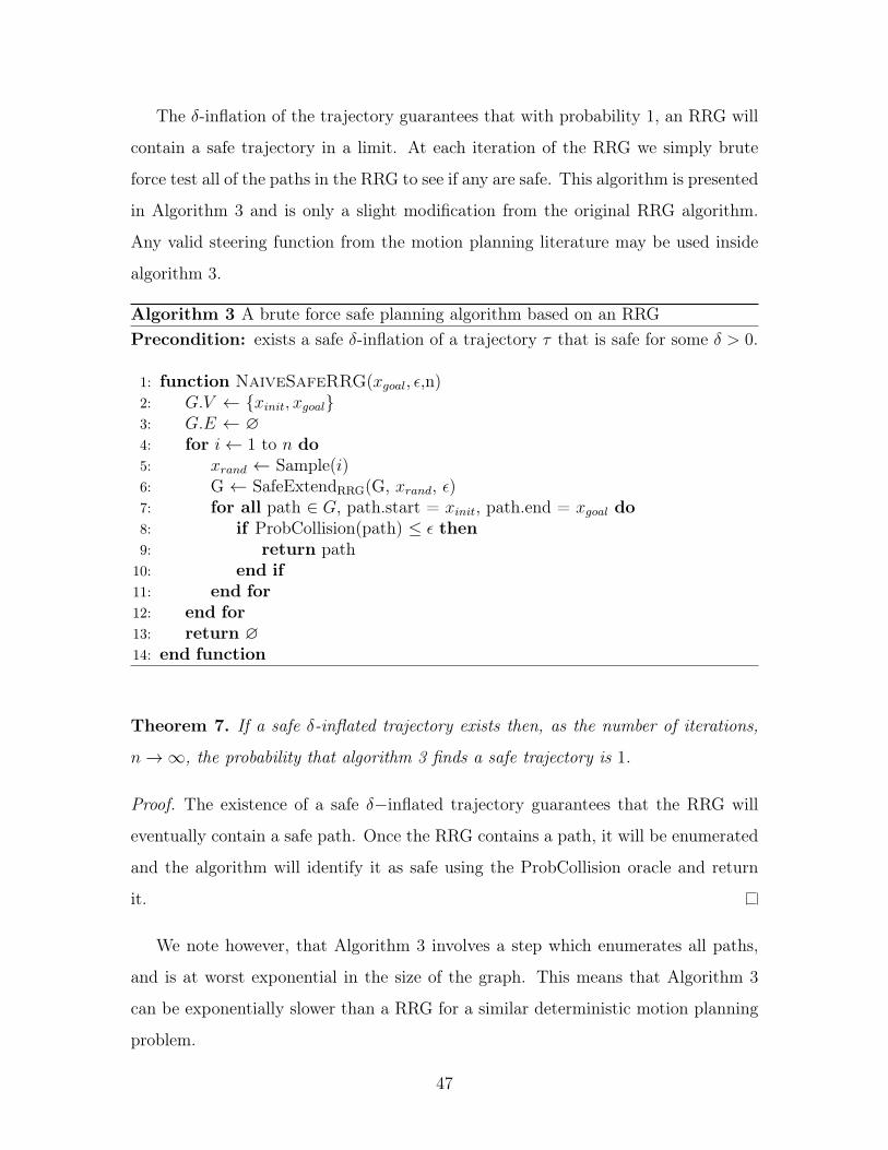
The 𝛿-inflation of the trajectory guarantees that with probability 1, an RRG will
contain a safe trajectory in a limit. At each iteration of the RRG we simply brute
force test all of the paths in the RRG to see if any are safe. This algorithm is presented
in Algorithm 3 and is only a slight modification from the original RRG algorithm.
Any valid steering function from the motion planning literature may be used inside
algorithm 3.
Algorithm 3 A brute force safe planning algorithm based on an RRGPrecondition: exists a safe 𝛿-inflation of a trajectory 𝜏 that is safe for some 𝛿 > 0.
1: function NaiveSafeRRG(𝑥𝑔𝑜𝑎𝑙, 𝜖,n)2: 𝐺.𝑉 ← {𝑥𝑖𝑛𝑖𝑡, 𝑥𝑔𝑜𝑎𝑙}3: 𝐺.𝐸 ← ∅4: for 𝑖← 1 to 𝑛 do5: 𝑥𝑟𝑎𝑛𝑑 ← Sample(𝑖)6: G ← SafeExtendRRG(G, 𝑥𝑟𝑎𝑛𝑑, 𝜖)7: for all path ∈ 𝐺, path.start = 𝑥𝑖𝑛𝑖𝑡, path.end = 𝑥𝑔𝑜𝑎𝑙 do8: if ProbCollision(path) ≤ 𝜖 then9: return path
10: end if11: end for12: end for13: return ∅14: end function
Theorem 7. If a safe 𝛿-inflated trajectory exists then, as the number of iterations,
𝑛→∞, the probability that algorithm 3 finds a safe trajectory is 1.
Proof. The existence of a safe 𝛿−inflated trajectory guarantees that the RRG will
eventually contain a safe path. Once the RRG contains a path, it will be enumerated
and the algorithm will identify it as safe using the ProbCollision oracle and return
it.
We note however, that Algorithm 3 involves a step which enumerates all paths,
and is at worst exponential in the size of the graph. This means that Algorithm 3
can be exponentially slower than a RRG for a similar deterministic motion planning
problem.
47
4.3 Hardness
We characterize the hardness of the approximate safe planning problem with PGDF
planning problem via a reduction to 3-SAT. The reduction is relatively robust–it does
not matter if we use the shadows used in chapter 3 or exact shadows. This section
contains only a proof outline.
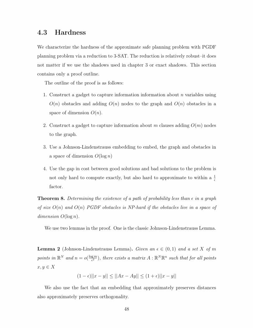
The outline of the proof is as follows:
1. Construct a gadget to capture information information about 𝑛 variables using
𝑂(𝑛) obstacles and adding 𝑂(𝑛) nodes to the graph and 𝑂(𝑛) obstacles in a
space of dimension 𝑂(𝑛).
2. Construct a gadget to capture information about 𝑚 clauses adding 𝑂(𝑚) nodes
to the graph.
3. Use a Johnson-Lindenstrauss embedding to embed, the graph and obstacles in
a space of dimension 𝑂(log 𝑛)
4. Use the gap in cost between good solutions and bad solutions to the problem is
not only hard to compute exactly, but also hard to approximate to within a 1𝜖
factor.
Theorem 8. Determining the existence of a path of probability less than 𝜖 in a graph
of size 𝑂(𝑛) and 𝑂(𝑛) PGDF obstacles is NP-hard if the obstacles live in a space of
dimension 𝑂(log 𝑛).
We use two lemmas in the proof. One is the classic Johnson-Lindenstrauss Lemma.
Lemma 2 (Johnson-Lindenstrauss Lemma). Given an 𝜖 ∈ (0, 1) and a set 𝑋 of 𝑚
points in R𝑁 and 𝑛 = 𝑜( log𝑚𝜖2
), there exists a matrix 𝐴 : R𝑁R𝑛 such that for all points
𝑥, 𝑦 ∈ 𝑋
(1− 𝜖)||𝑥− 𝑦|| ≤ ||𝐴𝑥− 𝐴𝑦|| ≤ (1 + 𝜖)||𝑥− 𝑦||
We also use the fact that an embedding that approximately preserves distances
also approximately preserves orthogonality.
48

Lemma 3. Given two orthogonal vectors 𝑥, 𝑦, and a corresponding Johnson-Lindenstrauss
embedding matrix 𝐴 for parameter 𝜖, and 𝜃 the angle between 𝐴𝑥,𝐴𝑦 then | cos 𝜃| =
𝑂(𝜖)
We will construct a graph and a set of obstacles that will capture a specific 3-SAT
problem. We have one axis that corresponds to the gadget number.
First we construct a gadget for capturing information about variables in the 3-SAT
formula. For convenience we place the "start“ node of the graph at the origin.
For each variable we assign a dimension and a variable node centered along this
new axis. We add one obstacle at the +1 coordinate on that dimension and one the
−1 coordinate. We add a node close to each obstacle. We connect these two nodes to
the previous and next variable nodes. This construction is illustrated in figure 4-2.
Figure 4-2: An example of a variable gadget
Now we add a gadget for every clause. We add a clause node at the next gadget
index. For every variable that appears unnegated we set the corresponding index
closer to +1. For each variable that appears negated we set the corresponding index
to −1.
Since the risk is paid for each obstacle only once, choosing a path through the
graph is equivalent to choosing an assignment of variables. If the risk is only paid
for as many obstacles as there are variables the 3SAT is satisfiable. Otherwise one
variable must be both true in some clauses and false in others.
49

50

Chapter 5
Safety in the Online Setting
So far in this thesis we have focused on guaranteeing safety in the following paradigm:
1. The episode begins
2. The robot gets information about its environment
3. The robot decides what action/trajectory to execute
4. The robot executes the action/trajectory
5. The episode ends
However, this paradigm rarely matches reality exactly. Instead of planning once,
robots often replan as they either deviate from the original trajectory or receive
additional sensor information.
This chapter examines how to guarantee safety in this more complicated setting.
5.1 Motivation
The safety guarantees developed earlier in this thesis, and in many other works, only
guarantees that during a single episode, the probability of collision between steps 1
and 5 is less an some fixed 𝜖 ∈ (0, 1). While these assumptions make it easier to
develop mathematical formalisms guaranteeing safety, they do not necessarily match
51

robot operation in practice. Ideally, we would guarantee that the lifetime probability
of collision of the robot is less than 𝜖 while giving the robot the flexibility to change
its desired trajectory upon receiving additional information. In fact we can show that
a system that obeys a safety guarantee in the simple paradigm can be made to collide
with probability arbitrarily close to 1 when used in a situation where it is allowed
to re-plan. Simply always following paths that are currently 𝜖-safe is not sufficient
to guarantee that the lifetime probability of collision remains low. This example is
illustrated in figure 5-1 and explained below.
First the robot finds a trajectory with collision probability 𝜖 and starts executing
it. As it travels by the first obstacle, it gets more informative observations regarding
the location of the obstacle. It now knows for sure it will not collide. Once it passes the
first obstacle it searches for a new trajectory with probability of collision 𝜖 of collision
and starts executing this. It repeats this process until it has reached its destination
or collides. It is important to note that this example is not convoluted and is not
far from how practical robot systems behave. It is quite common that robots obtain
better estimates of obstacles as they get closer and then re-plan less conservative
trajectories. It is also common for systems to merely require that any action they
take be safe instead of explicitly proving that the lifetime sequence of actions they will
take will be safe (especially when this sequence of actions is unknown when execution
begins). In doing so, these systems repeatedly take small risks without keeping track
of them, allowing the systems to collide more frequently than the safety guarantee
indicates.
Computation of the real probability of collision (approaching 1) in the scenario
presented in figure 5-1 follows quite directly. Say that during each step the probability
that the robot will collide with the first obstacle is 𝛼𝜖 and with the remaining obstacles
1− 𝛼𝜖. Let 𝐶𝑖 denote the event that the robot collides in the execution of step 𝑖.
52

0 5 10 15
-3
-2
-1
0
1
2
3
(a) The robot finds a trajectory with probability 𝜖 of collision and begins execution.
0 5 10 15
-3
-2
-1
0
1
2
3
(b) After having passed the first obstacle the robot uses all the new information it obtained tofind a new trajectory with probability of collision 𝜖. Since the robot now knows that the firstsegment of the trajectory was collision free, the fast and future portion of the trajectory have acombined collision probability of 𝜖.
Figure 5-1: An illustration about how a robot can be always taking an action that issafe, but still be guaranteed to eventually collide.
53

𝑃 (𝑐𝑜𝑙𝑙𝑖𝑠𝑖𝑜𝑛) = 𝑃 (𝐶1) + 𝑃 (𝐶𝐶1 )𝑃 (𝐶2|𝐶𝐶
1 ) + ...
= 𝛼𝜖 + (1− 𝛼𝜖)𝛼𝜖 + ... + (1− 𝛼𝜖)𝑛𝛼𝜖
In the limit of number of episodes this becomes
=𝛼𝜖
1− (1− 𝛼𝜖)
= 1
Since we clearly do not want our robots to collide with the environment with
probability one we need to understand what constitutes safe behavior in this “online”
setting where the robot is receiving a constant stream of information and is constantly
making decisions.
In this chapter of the thesis we develop a notions of policy safety and absolute
safety—a way of guaranteeing that the lifetime collision probability is less than a
fixed 𝜖, even when the robot has access to a constant stream of information and is
allowed to react to the new information.
5.2 Absolute Safety
First we formalize how our robotic system makes decisions. Let 𝑂𝑡 be the set of
observations by the robot (eg. sensor data) up to, but not including time 𝑡. Let 𝐴𝑡 be
the action that the robot commits to at 𝑡. If there is a processing delay, this action
might only be executed at a time 𝑡′ > 𝑡.
Definition 3 (policy). A policy 𝜋 : 𝑂𝑡 → 𝐴𝑡 is a function from observations to
actions.
This allows us to define a natural notion of safety for policies. Let 𝑈 be the event
that something unsafe (ex. a collision with an obstacle) occurs.
Definition 4 (Policy Safety). A policy 𝜋 is 𝜖-policy safe with respect to an event 𝑈
54
if the probability of 𝑈 under the policy is less than 𝜖.
𝑃 (𝑈 |𝜋) ≤ 𝜖
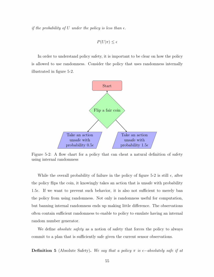
In order to understand policy safety, it is important to be clear on how the policy
is allowed to use randomness. Consider the policy that uses randomness internally
illustrated in figure 5-2.
Start
Flip a fair coin
Take an actionunsafe with
probability 0.5𝜖
Take an actionunsafe with
probability 1.5𝜖
Figure 5-2: A flow chart for a policy that can cheat a natural definition of safetyusing internal randomness
While the overall probability of failure in the policy of figure 5-2 is still 𝜖, after
the policy flips the coin, it knowingly takes an action that is unsafe with probability
1.5𝜖. If we want to prevent such behavior, it is also not sufficient to merely ban
the policy from using randomness. Not only is randomness useful for computation,
but banning internal randomness ends up making little difference. The observations
often contain sufficient randomness to enable to policy to emulate having an internal
random number generator.
We define absolute safety as a notion of safety that forces the policy to always
commit to a plan that is sufficiently safe given the current sensor observations.
Definition 5 (Absolute Safety). We say that a policy 𝜋 is 𝜖−absolutely safe if at
55
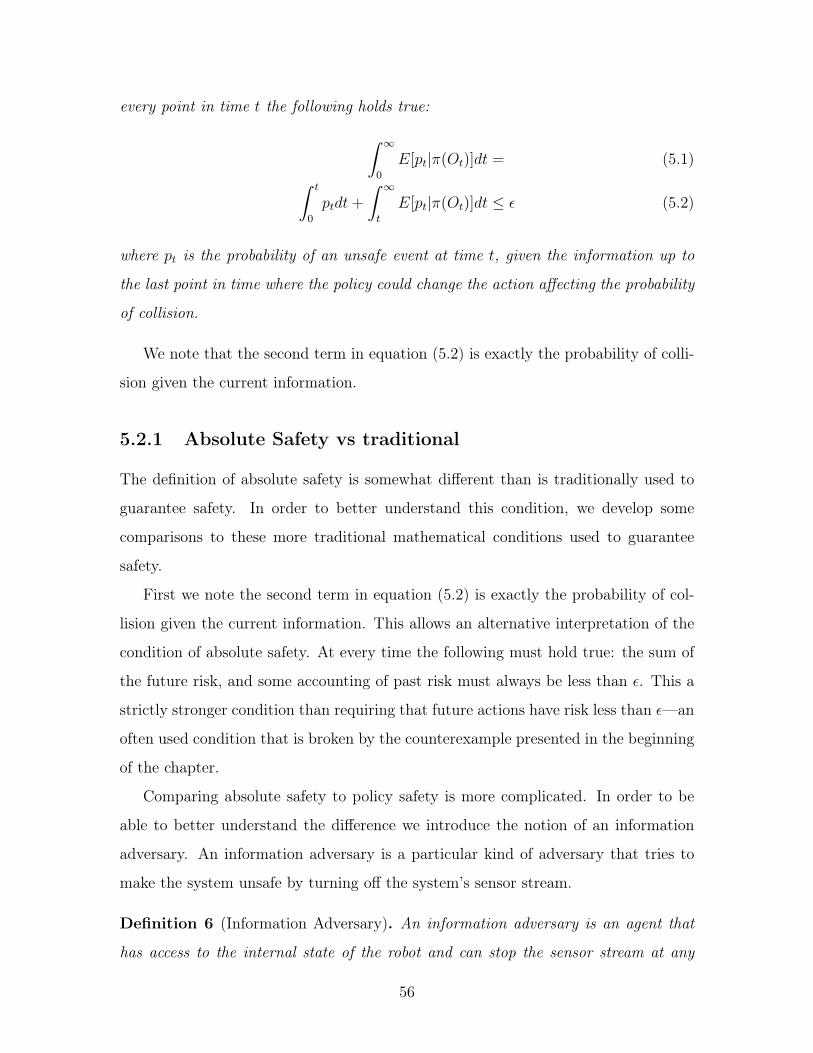
every point in time 𝑡 the following holds true:
∫︁ ∞
0
𝐸[𝑝𝑡|𝜋(𝑂𝑡)]𝑑𝑡 = (5.1)∫︁ 𝑡
0
𝑝𝑡𝑑𝑡 +
∫︁ ∞
𝑡
𝐸[𝑝𝑡|𝜋(𝑂𝑡)]𝑑𝑡 ≤ 𝜖 (5.2)
where 𝑝𝑡 is the probability of an unsafe event at time 𝑡, given the information up to
the last point in time where the policy could change the action affecting the probability
of collision.
We note that the second term in equation (5.2) is exactly the probability of colli-
sion given the current information.
5.2.1 Absolute Safety vs traditional
The definition of absolute safety is somewhat different than is traditionally used to
guarantee safety. In order to better understand this condition, we develop some
comparisons to these more traditional mathematical conditions used to guarantee
safety.
First we note the second term in equation (5.2) is exactly the probability of col-
lision given the current information. This allows an alternative interpretation of the
condition of absolute safety. At every time the following must hold true: the sum of
the future risk, and some accounting of past risk must always be less than 𝜖. This a
strictly stronger condition than requiring that future actions have risk less than 𝜖—an
often used condition that is broken by the counterexample presented in the beginning
of the chapter.
Comparing absolute safety to policy safety is more complicated. In order to be
able to better understand the difference we introduce the notion of an information
adversary. An information adversary is a particular kind of adversary that tries to
make the system unsafe by turning off the system’s sensor stream.
Definition 6 (Information Adversary). An information adversary is an agent that
has access to the internal state of the robot and can stop the sensor stream at any
56

point. The information adversary attempts to maximize the probability of an unsafe
event such as collision. In the notation used earlier in the chapter, an information
adversary can at any time 𝑡 ensure that 𝑂𝑡′ = 𝑂𝑡 for all 𝑡′ ≥ 𝑡.
The notion of an information adversary is what allows us to compare absolute
safety to policy safety. We use two theorems to compare the two notions of safety.
Theorem 9. 𝜖-absolute safety guarantees 𝜖-policy safety.
Theorem 10. A system that is 𝜖-policy safe at all times guarantees 𝜖-absolute safety.
More informally, absolute safety is a stronger condition than policy safety that
requires the system’s actions always be safe under the current information set.
The proof of the theorem 9 follows almost by definition.
Proof. Recall that we use 𝑈 to denote the unsafe event. We simply consider time 0,
the beginning of the episode. Absolute safety gives us the following conditions:
∞∫︁0
𝐸[𝑝𝑡|𝑂𝑡]𝑑𝑡 = 𝑃 (𝑈 | 𝜋) ≤ 𝜖
The proof of theorem 10 is by contradiction. If the theorem did not hold true, we
could explicitly construct a set of actions by the information adversary that would
make the policy unsafe. Absolute safety is stronger than policy safety in two ways:
1. No hedging bets. Absolute safety does not allow the robot to choose a risky
path half the time and a safe path half the time, even if the expected risk is
acceptable.
2. Relying on future information to make decisions. Absolute safety does not allow
a system to rely on receiving future observations.
Proof. Assume for the sake of contradiction that there exists a set of observations 𝑂
and a time 𝑡 for which absolute safety does not hold. That is to say that conditioned
57

on these observations
𝑡∫︁0
𝑝𝑡𝑑𝑡 +
∞∫︁𝑡
𝐸[𝑝𝑡 | 𝜋]𝑑𝑡 > 𝜖
Let the information adversary stop the flow of information to the robot at time 𝑡.
Let 𝐴1 de note the event that the system fails during times (0, 𝑡] and 𝐴2 denote the
event that the sy stems fails during times (𝑡,∞). We note that a system can fail at
most once, so 𝐴1, 𝐴2 are exclusive.
Utilizing the fact that∞∫︀𝑡
𝐸[𝑝𝑡|𝑂]𝑑𝑡 = 𝑃 (𝐴2|𝑂) and𝑡∫︀0
𝑝𝑡 | 𝑂𝑑𝑡 = 𝑃 (𝐴1 | 𝑂), we
get that the probability of failure 𝑃 (𝐴1 ∪ 𝐴2) = 𝑃 (𝐴1) + 𝑃 (𝐴2) ≥ 𝜖 violating our
assumption that the system is policy safe under the set of observations 𝑂.
5.2.2 Absolute Safety using Shadows
In this section we examine how to augment the algorithm in chapter 3 to guarantee
absolute safety. Recall that absolute safety is the following condition:
𝑡∫︁0
𝑝𝑡𝑑𝑡 +
∞∫︁𝑡
𝐸[𝑝𝑡 | 𝜋]𝑑𝑡 ≤ 𝜖
Alternatively using the fact that the second term is simply the future probability
of collision given the current information we get the following condition: (Note that
𝑈 is the collision event)
𝑡∫︁0
𝑝𝑡𝑑𝑡 + 𝑃 (𝑈) ≤ 𝜖
𝑃 (𝑈) is exactly the probability of collision computed in algorithm 2. The integral
in the first part can be computed using information available at the current time.
This leads to a modification that can allow us to certify that a system is safe under
replanning. This leads to the following modification to algorithm 2 that guarantees
58

𝜖-absolute safety:
1. Compute 𝜖1 =𝑡∫︀0
𝑝𝑡𝑑𝑡
2. Verify that any new proposed trajectory has probability of collision less than
𝜖− 𝜖1
If the trajectory chosen always passes the above safety check, the policy is guaranteed
to be 𝜖-absolutely safe.
5.3 Conclusion
Guaranteeing safety in the online setting can be rather nuanced and identifying de-
sired behavior can be difficult. For example, policy safety allows the system to take
actions that are known to be risky. Absolute safety and the information adversary
model on the other hand, can be too restrictive. We hope that future work will take
care to define safe behavior in a manner appropriate for the application.
59

60

Chapter 6
Conclusion
The contributions of this thesis can be split into two halves. The first half consists
of contributions of a mathematical nature. The thesis presents a way of quantifying
the quality of estimated shapes through models of random geometry and shadows.
It presents the PGDF model of random polytopes and describes how to compute
shadows of PGDF polytopes. For arbitrary distributions over half-spaces we show
how to find probability of intersection. We characterize the existence and uniqueness
of 𝜖-shadows for arbitrary distributions as well.
The second half presents algorithms that utilize the mathematics developed in the
first half. We present an efficient algorithm that an be used to bound the probability
of collision for a trajectory. We also discuss issues with generalizing our algorithm
to guarantee safe operation in a setting with a continuous flow of sensor data. We
present a general method that can be used to guarantee safety in such settings.
6.1 Future Work Related to Safe Navigation
While the algorithm we presented for bounding probability of collision is exponentially
faster than the state of the art Monte-Carlo based methods, much work remains to
be done. The bounds computed by the algorithm are not tight, and there is hope
that they can be improved.
The algorithm presented in chapter 3 does not compute actual motion plans. We
61

hope that a practical algorithm for finding safe plans can be obtained. Finally, the
PGDF has some surprising behavior that was highlighted in chapter 2. We hope that
future work will develop better estimation methods and statistical models in order to
avoid the degenerate behavior shown in chapter 2.
6.2 General Future work
The main contribution of the work is towards developing and applying a theory of
random geometry. Many systems, robotic and otherwise, must interact with geometry
in the environment. While we have many methods that estimate geometry based on
noisy observations, we often lack a rigorous understanding of how these methods
perform as statistical estimators [7, 19]. Understanding the mathematics behind
random geometry will not only help us understand how our current methods perform,
but also how to design better methods.
As demonstrated in this thesis, a better understanding of random geometry allows
us to efficiently reason about uncertainty in our estimates of geometry. In this thesis
we used this information to compute the probability that a particular robot trajectory
would collide with a set of estimated obstacles. This information could be used for
other applications as well. If we desired to improve our estimates of obstacles, this
information could inform us as to which observations would yield the most valuable
information. Perhaps this information can be used to devise grasping strategies that
are robust to the uncertainty in the estimates of the geometry.
Finally this thesis demonstrated that reasoning about uncertainty in this frame-
work can be done efficiently. Many problems in robotics that require reasoning about
uncertainty are provably hard. Restricting the problem in question to a specific distri-
bution of obstacles, and examining the underlying mathematics led to a very simple,
efficient approximation algorithm. In fact, the proposed algorithm is barely slower
than its equivalent for the deterministic setting. Hopefully understanding the math-
ematics behind random geometry will give us insight to what actually makes these
problems computationally hard, and suggest ways to get around the fundamental
62

computational restrictions at little practical cost.
63

64

Appendix A
Geometry and Vector Space Primer
The methods of bounding random geometry presented in this thesis require under-
standing the relationship between geometry in the space that robots operate in (usu-
ally R3) and the space of half-space parameters of geometry over R𝑛 (the dual space).
Duality in convex geometry studies precisely this when examining half-spaces (sets
of the form 𝛼𝑇𝑥 ≤ 0). The dual of the vector space R𝑛 is defined by the map that
sends the half-space 𝛼𝑇𝑥 ≤ 0 to 𝛼. The space of parameters 𝛼 of half-spaces over R𝑛
is called the dual space.
Throughout this thesis we use homogeneous coordinates, embedding the point
< 𝑥1, ...𝑥𝑛 >∈ R𝑛 as < 𝑥1, ...𝑥𝑛, 1 >∈ R𝑛+1. We can undo this mapping by sending
any point < 𝑥1....𝑥𝑛, 𝑥𝑛+1 > to 1𝑥𝑛+1
< 𝑥1, ..., 𝑥𝑛 >. This proves convenient as it allows
us write an equation such as 𝛼𝑇𝑥 ≤ 𝑏 compactly as < 𝛼1, ..., 𝛼𝑛,−𝑏 >𝑇 𝑥 ≤ 0 and
describe affine transformations on the original coordinates as linear transformations
(as matrices) on homogeneous coordinates.
While an in depth discussion we refer to Boyd et al. [3], we introduce the minimal
set of dual geometry concepts necessary to understand the developments in this thesis.
We discuss polar cones, dual cones, norm cones and dual norms.
65
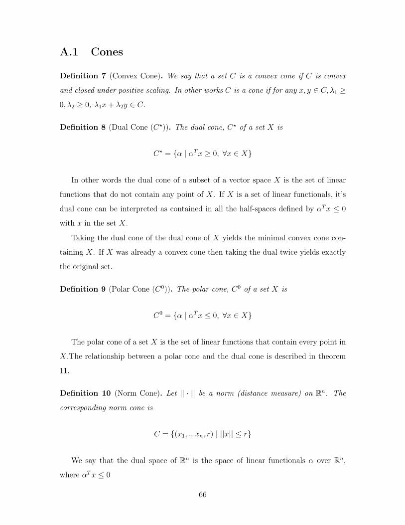
A.1 Cones
Definition 7 (Convex Cone). We say that a set 𝐶 is a convex cone if 𝐶 is convex
and closed under positive scaling. In other works 𝐶 is a cone if for any 𝑥, 𝑦 ∈ 𝐶, 𝜆1 ≥
0, 𝜆2 ≥ 0, 𝜆1𝑥 + 𝜆2𝑦 ∈ 𝐶.
Definition 8 (Dual Cone (𝐶⋆)). The dual cone, 𝐶⋆ of a set 𝑋 is
𝐶⋆ = {𝛼 | 𝛼𝑇𝑥 ≥ 0, ∀𝑥 ∈ 𝑋}
In other words the dual cone of a subset of a vector space 𝑋 is the set of linear
functions that do not contain any point of 𝑋. If 𝑋 is a set of linear functionals, it’s
dual cone can be interpreted as contained in all the half-spaces defined by 𝛼𝑇𝑥 ≤ 0
with 𝑥 in the set 𝑋.
Taking the dual cone of the dual cone of 𝑋 yields the minimal convex cone con-
taining 𝑋. If 𝑋 was already a convex cone then taking the dual twice yields exactly
the original set.
Definition 9 (Polar Cone (𝐶0)). The polar cone, 𝐶0 of a set 𝑋 is
𝐶0 = {𝛼 | 𝛼𝑇𝑥 ≤ 0, ∀𝑥 ∈ 𝑋}
The polar cone of a set 𝑋 is the set of linear functions that contain every point in
𝑋.The relationship between a polar cone and the dual cone is described in theorem
11.
Definition 10 (Norm Cone). Let || · || be a norm (distance measure) on R𝑛. The
corresponding norm cone is
𝐶 = {(𝑥1, ...𝑥𝑛, 𝑟) | ||𝑥|| ≤ 𝑟}
We say that the dual space of R𝑛 is the space of linear functionals 𝛼 over R𝑛,
where 𝛼𝑇𝑥 ≤ 0
66

*C0
C
Figure A-1: The dual cone of the blue blob
67
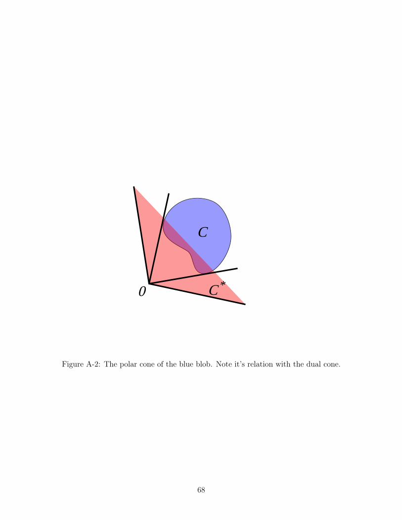
*C0
C
Figure A-2: The polar cone of the blue blob. Note it’s relation with the dual cone.
68
A.2 Useful Theorems about dual and polar Cones
Theorem 11. Let 𝐶⋆ be the dual cone of 𝑋, and 𝐶0 the polar cone of 𝑋. Then
𝐶⋆ = −𝐶0
Theorem 12. Let 𝐶 be the norm cone corresponding to || · ||. Then the dual cone,
𝐶⋆ is the norm cone with norm || · ||⋆, the dual norm of || · ||
A.3 Dual Norms
Definition 11 (Dual Norm (|| · ||⋆)). The dual norm of || · || is ||𝑥||⋆ = sup𝑦{𝑦𝑇𝑥 |
||𝑦|| ≤ 1}
Theorem 13. Let ||𝑥|| =√𝑥𝑇Σ𝑥 for Σ ≻ 0. Then ||𝑦||⋆ =
√︀𝑦𝑇Σ−1𝑦
Proof. We simply apply the KKT conditions to the definition of a dual norm.
||𝑦||⋆ = sup(𝑥𝑇𝑦 | ||𝑥|| ≤ 1)
Now we apply the KKT conditions
0 = ∇(𝑥𝑇𝑦 − 𝜆(√𝑥𝑇Σ𝑥− 1))
0 = 𝑦 − 2𝜆Σ𝑥
2√𝑥𝑇Σ𝑥
Since our problem is of a linear function over a convex domain our solution will lie on
the boundary of the domain. This implies that ||𝑥|| = 1 and allows us to solve for 𝑥.
𝑥⋆ = 𝜆Σ−1𝑦
=Σ−1𝑦√︀
𝑦𝑇Σ−1ΣΣ−1𝑦
=Σ−1𝑦√︀𝑦𝑇Σ−1𝑦
69

Now we can evaluate the supremum
sup(𝑥𝑇𝑦 | ||𝑥|| ≤ 1) = 𝑥⋆𝑇𝑦
=𝑦𝑇Σ−1𝑦√︀𝑦𝑇Σ−1𝑦
=√︀
𝑦𝑇Σ−1𝑦
70

Bibliography
[1] Haoyu Bai, David Hsu, Wee Sun Lee, and Vien A Ngo. Monte carlo valueiteration for continuous-state pomdps. In Algorithmic foundations of roboticsIX, pages 175–191. Springer, 2010.
[2] Christopher M Bishop. Pattern recognition. Machine Learning, 128:1–58, 2006.
[3] Stephen Boyd and Lieven Vandenberghe. Convex optimization. Cambridge uni-versity press, 2004.
[4] Adam Bry and Nicholas Roy. Rapidly-exploring random belief trees for motionplanning under uncertainty. In Robotics and Automation (ICRA), 2011 IEEEInternational Conference on, pages 723–730. IEEE, 2011.
[5] John Canny and John Reif. Lower bounds for shortest path and related problems.In Proc. 28th Ann. IEEE Symp. Found. Comp. Sci, volume 49, page 60, 1987.
[6] Gregory Dudek, Kathleen Romanik, and Sue Whitesides. Localizing a robot withminimum travel. SIAM Journal on Computing, 27(2):583–604, 1998.
[7] Olivier Faugeras, Quang-Tuan Luong, and Theo Papadopoulo. The geometry ofmultiple images: the laws that govern the formation of multiple images of a sceneand some of their applications. MIT press, 2004.
[8] Mzuri Handlin. Conic sections beyond R2.https://www.whitman.edu/Documents/Academics/Mathematics/Handlin.pdf.Accessed: 2017-2-16.
[9] Kaijen Hsiao, Leslie Pack Kaelbling, and Tomas Lozano-Perez. Graspingpomdps. In Robotics and Automation, 2007 IEEE International Conference on,pages 4685–4692. IEEE, 2007.
[10] Lucas Janson, Edward Schmerling, and Marco Pavone. Monte carlo motionplanning for robot trajectory optimization under uncertainty. In InternationalSymposium on Robotics Research, Sestri Levante, Italy, September 2015. ToAppear.
[11] Lucas Janson, Edward Schmerling, and Marco Pavone. Monte carlo motionplanning for robot trajectory optimization under uncertainty. arXiv preprintarXiv:1504.08053, 2015.
71

[12] Leslie Pack Kaelbling and Tomás Lozano-Pérez. Integrated task and motionplanning in belief space. The International Journal of Robotics Research, 32(9-10):1194–1227, 2013.
[13] Leslie Pack Kaelbling, Michael L Littman, and Anthony R Cassandra. Planningand acting in partially observable stochastic domains. Artificial intelligence, 101(1):99–134, 1998.
[14] Sertac Karaman and Emilio Frazzoli. Incremental sampling-based algorithms foroptimal motion planning. Robotics Science and Systems VI, 104, 2010.
[15] Hanna Kurniawati, David Hsu, and Wee Sun Lee. Sarsop: Efficient point-basedpomdp planning by approximating optimally reachable belief spaces. In Robotics:Science and systems, volume 2008. Zurich, Switzerland., 2008.
[16] Alex Lee, Yan Duan, Sachin Patil, John Schulman, Zoe McCarthy, Jur van denBerg, Ken Goldberg, and Pieter Abbeel. Sigma hulls for gaussian belief spaceplanning for imprecise articulated robots amid obstacles. In Intelligent Robotsand Systems (IROS), 2013 IEEE/RSJ International Conference on, pages 5660–5667. IEEE, 2013.
[17] Omid Madani, Steve Hanks, and Anne Condon. On the undecidability of proba-bilistic planning and infinite-horizon partially observable markov decision prob-lems. In AAAI/IAAI, pages 541–548, 1999.
[18] Anirudha Majumdar and Russ Tedrake. Funnel libraries for real-time robustfeedback motion planning. arXiv preprint arXiv:1601.04037, 2016.
[19] Richard A Newcombe, Shahram Izadi, Otmar Hilliges, David Molyneaux, DavidKim, Andrew J Davison, Pushmeet Kohi, Jamie Shotton, Steve Hodges, andAndrew Fitzgibbon. Kinectfusion: Real-time dense surface mapping and track-ing. In Mixed and augmented reality (ISMAR), 2011 10th IEEE internationalsymposium on, pages 127–136. IEEE, 2011.
[20] Christos H Papadimitriou and John N Tsitsiklis. The complexity of markovdecision processes. Mathematics of operations research, 12(3):441–450, 1987.
[21] Joelle Pineau, Geoff Gordon, Sebastian Thrun, et al. Point-based value iteration:An anytime algorithm for pomdps. In IJCAI, volume 3, pages 1025–1032, 2003.
[22] Carl Edward Rasmussen. Gaussian processes for machine learning. 2006.
[23] John H Reif. Complexity of the mover’s problem and generalizations. In Foun-dations of Computer Science, 1979., 20th Annual Symposium on, pages 421–427.IEEE, 1979.
[24] Dorsa Sadigh and Ashish Kapoor. Safe control under uncertainty with prob-abilistic signal temporal logic. In Proceedings of Robotics: Science and Sys-tems, Ann Arbor, Michigan, June 2016. doi: 10.15607/RSS.2016.XII.017. URLhttp://www.roboticsproceedings.org/rss12/p17.html.
72

[25] Edward Schmerling and Marco Pavone. Evaluating trajectory collision probabil-ity through adaptive importance sampling for safe motion planning. In Proceed-ings of Robotics: Science and Systems, Cambridge, Massachusetts, July 2017.doi: 10.15607/RSS.2017.XIII.068.
[26] David Silver and Joel Veness. Monte-carlo planning in large pomdps. In Advancesin neural information processing systems, pages 2164–2172, 2010.
[27] Trey Smith. Probabilistic planning for robotic exploration. Carnegie MellonUniversity, 2007.
[28] Kiril Solovey and Dan Halperin. On the hardness of unlabeled multi-robot motionplanning. The International Journal of Robotics Research, 35(14):1750–1759,2016.
[29] Jacob Steinhardt and Russ Tedrake. Finite-time regional verification of stochasticnon-linear systems. The International Journal of Robotics Research, 31(7):901–923, 2012.
[30] Russ Tedrake. Lqr-trees: Feedback motion planning on sparse randomized trees.2009.
[31] Georgios Theocharous and Leslie P Kaelbling. Approximate planning in pomdpswith macro-actions. In Advances in Neural Information Processing Systems,pages 775–782, 2004.
[32] Mark M Tobenkin, Ian R Manchester, and Russ Tedrake. Invariant funnelsaround trajectories using sum-of-squares programming. IFAC Proceedings Vol-umes, 44(1):9218–9223, 2011.
[33] Craig Tovey and Sven Koenig. Gridworlds as testbeds for planning with incom-plete information. In AAAI/IAAI, pages 819–824, 2000.
73