algorithms and techniques for managing...
TRANSCRIPT

ALGORITHMS AND TECHNIQUES FOR MANAGING EXTENSIBILITY IN
CYBER-PHYSICAL SYSTEMS
By
Subhav Pradhan
Dissertation
Submitted to the Faculty of the
Graduate School of Vanderbilt University
in partial fulfillment of the requirements
for the degree of
DOCTOR OF PHILOSOPHY
in
Computer Science
December, 2016
Nashville, Tennessee
Approved:
Aniruddha S. Gokhale, Ph.D.
Abhishek Dubey, Ph.D.
Gabor Karsai, Ph.D.
Janos Sztipanovits, Ph.D.
Akram Hakiri, Ph.D.

To my beloved late grandparents,Jitendra Lal Maskey, Hiranneshwor Man Pradhan, and Badan Pradhan
and
To my beloved grandmother, Sushila Maskey
ii

ACKNOWLEDGMENTS
This dissertation would not have been possible without the tremendous amount of guid-
ance and support I received from my advisors, colleagues, friends, and family.
First of all, I would like to express my sincere gratitude to my advisors Dr. Aniruddha
Gokhale and Dr. Abhishek Dubey; I am eternally grateful for their unwavering support,
guidance, and patience throughout my years as a graduate student at Vanderbilt University.
After a challenging first year, Dr. Gokhale provided me the moral support and intellectual
guidance I desperately needed to pursue and realize my dream. I also owe all of my success
to Dr. Dubey for being an ever-present mentor who guided me through numerous research
ideas, projects, and papers.
I would like to thank Dr. Gabor Karsai, Dr. Janos Sztipanovits, and Dr. Akram Hakiri
for serving as members of my dissertation committee and providing me with valuable in-
sights and feedback. I am especially grateful for the guidance and mentorship provided
by Dr. Karsai over the years. I would also like to thank Dr. William Otte, Dr. Tihamer
Levendovszky, and Dr. Douglas Schmidt for supporting various aspects of my research.
My graduate school experience would not have been successful without the support
of my friends. The countless feedback and support I received from DOC group friends –
Kyoungho, Prithviraj, Faruk, Shashank, Shweta, Yogesh, Anirban, and Shunxing – helped
me shape my research. The weekly soccer games and pool outings with friends outside
the DOC group – Dhiraj, Piyush, Pranita, Sagar, Bhumika, Krishen, Brandon, Dima, and
David – helped me weather the frustrations that comes with the chaos of graduate school.
A special mention to a very special friend, Manisha Thapa; the smartest and the wittiest
person that I have ever known who was always there for me, never failing to provide moral
support whenever I needed. I would not have been able to achieve this feat without her.
Although oceans apart, my parents, Dr. Rajendra Man Pradhan and Ameeta Pradhan,
have been a constant source of comfort and encouragement. It is their support and endless
iii

effort that has helped me stay on track and rise regardless of the number of falls. I would
also like to thank my aunt Smreeti Maskey for always providing sound advice. Although
I cannot celebrate this achievement with my late grandfather Jitendra Lal Maskey, I know
he must be extremely proud of me. He has and always will be my eternal inspiration.
Finally, I would like to thank the Defense Advanced Projects Agency (DARPA), Air
Force Research Lab (AFRL), National Science Foundation (NSF), and Siemens Corporate
Technology for financially supporting various research projects that I have been part of
over the years at Vanderbilt University.
iv

TABLE OF CONTENTS
Page
DEDICATION . . . . . . . . . . . . . . . . . . . . . . . . . . . . . . . . . . . . . ii
ACKNOWLEDGMENTS . . . . . . . . . . . . . . . . . . . . . . . . . . . . . . . . iii
LIST OF TABLES . . . . . . . . . . . . . . . . . . . . . . . . . . . . . . . . . . . viii
LIST OF FIGURES . . . . . . . . . . . . . . . . . . . . . . . . . . . . . . . . . . . ix
Chapter
I. Introduction . . . . . . . . . . . . . . . . . . . . . . . . . . . . . . . . . . 1
I.1. History, Evolution and Emerging Trends in Distributed Computing 1I.2. Extensible CPS . . . . . . . . . . . . . . . . . . . . . . . . . . . 3
I.2.1. Extensible Systems . . . . . . . . . . . . . . . . . . . 4I.2.2. Evolution of Extensible Systems . . . . . . . . . . . . 5I.2.3. Extensibility in CPS . . . . . . . . . . . . . . . . . . . 6
I.3. Challenges for Extensible CPS . . . . . . . . . . . . . . . . . . 7I.4. Overview of Proposed Doctoral Research . . . . . . . . . . . . . 11
II. Background and Motivating Scenario . . . . . . . . . . . . . . . . . . . . 14
II.1. Target System Model . . . . . . . . . . . . . . . . . . . . . . . . 14II.2. Application Model . . . . . . . . . . . . . . . . . . . . . . . . . 15II.3. Failure Model . . . . . . . . . . . . . . . . . . . . . . . . . . . 16II.4. Motivating Scenario: Smart Emergency Response System . . . . 19
III. A Resilient Deployment and Reconfiguration Infrastructure to ManageDistributed Applications . . . . . . . . . . . . . . . . . . . . . . . . . . . 20
III.1. Motivation . . . . . . . . . . . . . . . . . . . . . . . . . . . . . 20III.2. Background and Problem Description . . . . . . . . . . . . . . . 21III.3. Key Considerations and Challenges . . . . . . . . . . . . . . . . 22III.4. A Resilient Deployment and Reconfiguration Infrastructure . . . 24
III.4.1. Solution Architecture . . . . . . . . . . . . . . . . . . 25III.4.2. Addressing Resilient D&C Challenges . . . . . . . . . 28
III.5. Experimental Results . . . . . . . . . . . . . . . . . . . . . . . . 29III.5.1. Testbed . . . . . . . . . . . . . . . . . . . . . . . . . . 30III.5.2. Node Failure During Deployment-time . . . . . . . . . 30III.5.3. Node Failure During Application Run-time . . . . . . . 30
III.6. Related Work . . . . . . . . . . . . . . . . . . . . . . . . . . . . 33III.7. Concluding Remarks . . . . . . . . . . . . . . . . . . . . . . . . 34
v

III.8. Related Publications . . . . . . . . . . . . . . . . . . . . . . . . 35
IV. Establishing Secure Interaction Across Distributed Applications . . . . . . 36
IV.1. Motivation . . . . . . . . . . . . . . . . . . . . . . . . . . . . . 36IV.2. Background and Problem Description . . . . . . . . . . . . . . . 37
IV.2.1. System Model . . . . . . . . . . . . . . . . . . . . . . 37IV.2.2. OMG DDS Overview . . . . . . . . . . . . . . . . . . 37IV.2.3. Problem Statement . . . . . . . . . . . . . . . . . . . . 38
IV.3. Solution Approach . . . . . . . . . . . . . . . . . . . . . . . . . 39IV.3.1. Secure Transport . . . . . . . . . . . . . . . . . . . . . 40IV.3.2. A Secure Discovery Mechanism . . . . . . . . . . . . . 43
IV.4. Experimental Evaluation . . . . . . . . . . . . . . . . . . . . . . 47IV.4.1. Experimental Setup . . . . . . . . . . . . . . . . . . . 47IV.4.2. Secure Transport Network Utilization . . . . . . . . . . 48
IV.5. Related Work . . . . . . . . . . . . . . . . . . . . . . . . . . . . 49IV.6. Concluding Remarks . . . . . . . . . . . . . . . . . . . . . . . . 51IV.7. Related Publication . . . . . . . . . . . . . . . . . . . . . . . . 52
V. Achieving Resilience in Extensible CPS via Self-Reconfiguration . . . . . 53
V.1. Motivation . . . . . . . . . . . . . . . . . . . . . . . . . . . . . 53V.2. Background and Problem Description . . . . . . . . . . . . . . . 56
V.2.1. Goal-based System Description . . . . . . . . . . . . . 56V.2.2. Resource Model . . . . . . . . . . . . . . . . . . . . . 58V.2.3. Deployment Model . . . . . . . . . . . . . . . . . . . . 59V.2.4. Problem Statement . . . . . . . . . . . . . . . . . . . . 61
V.3. Solution Approach . . . . . . . . . . . . . . . . . . . . . . . . . 63V.3.1. Overview of the Solution Approach . . . . . . . . . . . 63V.3.2. Design-time Resilience Analysis Tool . . . . . . . . . . 64V.3.3. Runtime Infrastructure for Self-Reconfiguration . . . . 69
V.4. Case Study: Fractionated Satellite Cluster . . . . . . . . . . . . . 77V.4.1. Scenario . . . . . . . . . . . . . . . . . . . . . . . . . 77V.4.2. Resilience Metrics Calculation . . . . . . . . . . . . . 79V.4.3. Runtime Self-Reconfiguration Mechanism Demonstra-
tion . . . . . . . . . . . . . . . . . . . . . . . . . . . . 84V.4.4. Runtime Self-Reconfiguration Mechanism Evaluation . 84
V.5. Related Work . . . . . . . . . . . . . . . . . . . . . . . . . . . . 86V.6. Concluding Remarks . . . . . . . . . . . . . . . . . . . . . . . . 88V.7. Related Publications . . . . . . . . . . . . . . . . . . . . . . . . 89
VI. A Holistic Solution for Managing Extensible CPS . . . . . . . . . . . . . 90
VI.1. Motivation . . . . . . . . . . . . . . . . . . . . . . . . . . . . . 90VI.2. Problem Description . . . . . . . . . . . . . . . . . . . . . . . . 92VI.3. Solution Approach . . . . . . . . . . . . . . . . . . . . . . . . . 93
VI.3.1. Overview of the Solution Approach . . . . . . . . . . . 93
vi

VI.3.2. The CHARIOT Design Layer . . . . . . . . . . . . . . 97VI.3.3. The CHARIOT Data Layer . . . . . . . . . . . . . . . 105VI.3.4. The CHARIOT Management Layer . . . . . . . . . . . 110
VI.4. Implementation and Evaluation . . . . . . . . . . . . . . . . . . 126VI.4.1. CHARIOT Runtime Implementation . . . . . . . . . . 127VI.4.2. Experimental Evaluation . . . . . . . . . . . . . . . . . 130
VI.5. Related Work . . . . . . . . . . . . . . . . . . . . . . . . . . . . 140VI.5.1. Redundancy-based Strategies . . . . . . . . . . . . . . 140VI.5.2. Reconfiguration-based Strategies . . . . . . . . . . . . 141
VI.6. Concluding Remarks . . . . . . . . . . . . . . . . . . . . . . . . 142VI.7. Related Publications . . . . . . . . . . . . . . . . . . . . . . . . 144
VII. Concluding Remarks and Future Work . . . . . . . . . . . . . . . . . . . . 145
VII.1.Summary of Research Contributions . . . . . . . . . . . . . . . 146VII.2.Future Work: Towards a Generic Computation Model . . . . . . 147
VII.2.1.Background and Problem Description . . . . . . . . . . 148VII.2.2.Proposed Solution: A Generic Computation Model . . . 153
VII.3.Summary of Publications . . . . . . . . . . . . . . . . . . . . . 157
REFERENCES . . . . . . . . . . . . . . . . . . . . . . . . . . . . . . . . . . . . . 161
vii

LIST OF TABLES
Table Page
1. Differences between CPS and Extensible CPS. . . . . . . . . . . . . . . 7
2. Properties of Extensible CPS. . . . . . . . . . . . . . . . . . . . . . . . 8
3. Deployment and Configuration Stages . . . . . . . . . . . . . . . . . . . 27
4. Entities involved in the Secure Discovery Mechanism. . . . . . . . . . . 45
5. Network Utilization Calculations for IPv6 and for Secure Transport tun-neled through an IPv4 network. . . . . . . . . . . . . . . . . . . . . . . 49
6. Constraint Primitives implemented using Z3 Solver [26] Python APIs. . . 66
7. Sequence of Events used for evaluation of CPC algorithm. . . . . . . . . 131
8. Different Categories of Resources in a Smart City Platform. . . . . . . . 150
9. Different Computing Patterns for a Smart City Platform. . . . . . . . . . 152
viii

LIST OF FIGURES
Figure Page
1. Evolution of Distributed Computing Paradigm. . . . . . . . . . . . . . . 2
2. CPS Feedback Control Loop. . . . . . . . . . . . . . . . . . . . . . . . 3
3. Target System Model comprising Component-based Application Modelfor Extensible CPS. . . . . . . . . . . . . . . . . . . . . . . . . . . . . . 15
4. Smart Emergency Response System with Different Physical Domains. . . 19
5. Orchestrated Deployment Approach in LE-DAnCE [82]. . . . . . . . . . 21
6. Overview of a Resilient D&C Infrastructure. . . . . . . . . . . . . . . . 24
7. Architecture of a Resilience D&C Infrastructure. . . . . . . . . . . . . . 25
8. Three-node Deployment and Configuration Setup. . . . . . . . . . . . . 26
9. Deployment Time Node Failure. . . . . . . . . . . . . . . . . . . . . . . 31
10. Runtime Node Failure. . . . . . . . . . . . . . . . . . . . . . . . . . . . 32
11. OpenDDS Centralized Discovery Mechanism . . . . . . . . . . . . . . . 38
12. Topic based application interaction in OMG DDS . . . . . . . . . . . . . 39
13. Discovery Architecture. Table 4 describes the entities shown in this figure. 46
14. Sequence Diagram illustrating the process of (1) Data Writer Creation,and (2) Data Reader Association. . . . . . . . . . . . . . . . . . . . . . 46
15. Use case scenario: Two DDS Applications with Different Security Labels. 47
16. App-1 Log Snippet which shows that App-1 only receives messages pub-lished by itself and not from App-2 since the latter has higher SecurityLabel. . . . . . . . . . . . . . . . . . . . . . . . . . . . . . . . . . . . . 48
17. App-2 Log Snippet which shows that App-2 receives messages pub-lished by both itself and App-1 since it has higher Security Label thanApp-1. . . . . . . . . . . . . . . . . . . . . . . . . . . . . . . . . . . . 48
ix

18. Distributed Deployment of Applications with mixed-criticality on a Frac-tionated Satellite Cluster. . . . . . . . . . . . . . . . . . . . . . . . . . . 54
19. Tasks performed by components of the Cluster Flight Application. Forthese tasks, the subscript represents the ID of the node onto which a taskis deployed. The total latency of the interaction C1
1 →M2N represents the
total latency between receiving the scatter command and activating thethrusters. This interaction pathway is in bold. . . . . . . . . . . . . . . . 55
20. Functional Decomposition Graph for a simple two-application System. . 57
21. Overview of the Solution Approach. . . . . . . . . . . . . . . . . . . . . 63
22. Overview of the distributed self-reconfiguration infrastructure with De-ployment and Reconfiguration action sequences. Initial deployment istriggered when a user/system integrator generates and stores the config-uration space and the initial configuration point for a system using thedesign-time modeling tool. Once this is done, a Resilience Engine (RE)is invoked to instigate initial deployment. The RE then computes the re-quired deployment actions and stores them in the database. At this point,the Deployment Managers (DMs) that are responsible for taking theseactions are notified after which they execute those commands locally tocomplete initial deployment. Reconfiguration is similar, however, unlikea user/system integrator instigating the process, it is a monitor that in-stigates the process by logging information about any detected failure tothe database and invoking the RE. This should only be done by a sin-gle monitor, as such we dedicate this task to the leader monitor, i.e., themonitor running on the leader node. . . . . . . . . . . . . . . . . . . . . 70
23. Software Model Design using GME [55] based Modeling Language. . . 78
24. System Configuration after Initial Deployment of Model in Figure 23. . . 80
25. Resilience Metrics (left) and corresponding computation time (right) fordifferent variation of system model presented in Figure 23. A representsthe default model (shown in Figure 23), B represents a model in which aGPU device is removed from SatAlpha, C represents a model in whicha HR_Camera is added to SatBeta, D represents a model in which a newnode similar to SatGamma is added to the system, and E represents amodel in which a new node similar to SatAlpha is added to the system. . 82
26. System configuration after recovering from ImageProcessor componentfailure in node SatBeta. Compare it to the initial configuration shown inFigure 24. . . . . . . . . . . . . . . . . . . . . . . . . . . . . . . . . . . 83
x

27. Configuration computation time for failures in a simple model (left) andaverage configuration computation time for four failures in different sys-tem models (right). The different system models have increasing com-plexity; A has 3 nodes and 13 components, B has 5 nodes and 19 com-ponents, C has 8 nodes and 28 components, D has 10 nodes and 34components, E has 12 nodes and 40 components, F has 15 nodes and 49components, and G has 18 nodes and 58 components. . . . . . . . . . . 85
28. An Overview of the Parking Management System Case Study. . . . . . . 91
29. The Layered Architecture of CHARIOT. . . . . . . . . . . . . . . . . . 94
30. Reconfiguration Triggers associated with Failure Management and Op-erations Management. . . . . . . . . . . . . . . . . . . . . . . . . . . . 96
31. CHARIOT-ML Modeling Concepts and their Dependencies. . . . . . . . 98
32. Parking System Description for the example shown in figure 28. . . . . . 99
33. Snippet of Node Categories and Node Templates Declarations. . . . . . . 100
34. Snippet of Smart Parking Goal Description Comprising Objectives andReplication Constraints. . . . . . . . . . . . . . . . . . . . . . . . . . . 101
35. Example Redundancy Patterns for Functionality F1. The CSn_m entitiesrepresent consensus service providers. . . . . . . . . . . . . . . . . . . . 102
36. Snippet of Functionalities and Corresponding Composition Declaration. . 104
37. Snippet of Component Type Declaration. . . . . . . . . . . . . . . . . . 104
38. UML Class Diagrams for Schemas Used to Store System Information. . . 106
39. The Implementation Design of the CHARIOT Runtime. . . . . . . . . . 127
40. Default CPC Algorithm Performance. (Please refer to Table 7 for detailsabout each event shown in this graph.) . . . . . . . . . . . . . . . . . . . 132
41. Solution Pre-computation Time for CPC with LaRC. (The solution forfailure event i+1 is computed when the reconfiguration action for thefailure event i is being applied.) . . . . . . . . . . . . . . . . . . . . . . 134
42. Average Memory Consumption. . . . . . . . . . . . . . . . . . . . . . . 135
43. Average Network Bandwidth Consumption. . . . . . . . . . . . . . . . . 135
xi

44. Default CPC Algorithm Performance in Simulated Environment. (Pleaserefer to Table 7 for details about each event shown in this graph.) . . . . 136
45. Default CPC Algorithm Performance Comparison between Non-simulatedand Simulated Environments. (Please refer to Table 7 for details abouteach event shown in this graph.) . . . . . . . . . . . . . . . . . . . . . . 137
46. The Z3 Solver Time Jitter versus the corresponding Problem Complex-ity. (Please refer to Table 7 for details about each event shown in thisgraph.) . . . . . . . . . . . . . . . . . . . . . . . . . . . . . . . . . . . 138
47. Solution Computation Time for different Initial Deployment Scenarios. . 139
48. Breakdown of Total Constraint Encoding Time into Different Constraints. 139
49. A Smart City Platform comprising a single Computing Group Collectioncomposed of four different Computing Groups of three different categories.149
50. Different Types of Applications based on Resource requirement, Timingrequirement, Criticality, and Scale. . . . . . . . . . . . . . . . . . . . . . 151
51. A Computation Graph comprising Computation Tasks, Dataflows be-tween Tasks, an Event Source and a Data Source. . . . . . . . . . . . . . 154
52. Overview of the CHARIOT Component Model. . . . . . . . . . . . . . . 155
53. An Example Demonstrating interaction between a Component Assemblythat maps to a Storm Topology and a CHARIOT component. . . . . . . . 157
xii

CHAPTER I
INTRODUCTION
I.1 History, Evolution and Emerging Trends in Distributed Computing
Over the past decades, distributed computing paradigm has evolved from smaller and
mostly homogeneous clusters to the current notion of ubiquitous computing, which consists
of dynamic and heterogeneous resources in large scale; an outline of this evolution is pre-
sented in Figure 1. Although the history of distributed computing can be traced back to the
late 1960s and the early 1970s when ARPANET and ARPANET e-mail were invented, it
was only during the 1990s when early distributed systems came into prominence with the
introduction of client/server architecture. However, these early distributed systems were
small scale homogeneous clusters.
Starting the mid 2000s, distributed computing paradigm shifted towards utility comput-
ing. This transition was instigated by the introduction of grid computing [37], which is a
form of utility computing that provides scalability to achieve different kinds of high per-
formance computing. The main goal of grid computing was to enable coordinated resource
sharing between multi-institutional organizations resulting in distributed ownership of het-
erogenous resources. Towards the late 2000s, cloud computing [10] was introduced as a
different form of utility computing. Cloud computing is used to provide software, platform,
and infrastructure services to consumers without them having to worry about infrastructure
or maintenance cost. As such, unlike grid computing, scaling in cloud computing is geared
towards achieving high scalability computing that facilitates dynamic service elasticity.
Ubiquitous computing [59] represents the present and future of distributed computing
paradigm. It refers to a paradigm where computing resources are made available every-
where and anywhere. Although the term ubiquitous computing was coined by Mark Weiser
in 1991 [109], realization of these systems happened recently due to wider adaption and
1

Figure 1: Evolution of Distributed Computing Paradigm.
availability of wireless networking technologies and edge computing devices such as sin-
gle board computers, smart phones and tablets. Applications of ubiquitous computing has
evolved from mobile computing [36], which focuses on mobile devices connecting users to
networks (including the Internet) via wireless networking technologies, to the Internet of
Things (IoT) [13], which consists of “things" (devices) connected via the Internet.
Recent advancement of edge computing devices has resulted in sophisticated and re-
sourceful devices that are equipped with variety of sensors and actuators (for example, Intel
Edison module mounted on Arduino board1 compatible with various sensors available as
part of the Grove Starter Kit2). These devices can be used to connect physical world with
the cyber world [17, 25]. As such, the future of ubiquitous computing is cyber-physical in
nature, and therefore, Cyber-Physical Systems (CPS) will play a crucial role in the future
of ubiquitous computing. CPS are engineered systems that integrate cyber and physical
components, where cyber components include computation and communication resources
and physical components represent physical systems [56, 91]. CPS can be considered a
special type of ubiquitous system that combines control theory, communications, and real-
time computing with embedded applications that interact with the physical world [68]. As
shown in Figure 2, CPS can be considered feedback control loops in which the controllers
are cyber components that, based on desired behavior, use actuators to make changes to the
physical systems and sensors to monitor/observe those systems.
1https://www.arduino.cc/en/ArduinoCertified/IntelEdison2http://wiki.seeedstudio.com/wiki/Grove_-_Starter_Kit_v3
2

Figure 2: CPS Feedback Control Loop.
As shown in Figure 1, smart cities [31, 104] are a great exemplar of the future of ubiqui-
tous computing. A smart city will comprise heterogeneous resources for domains varying
from transportation, emergency response, power grid, etc. Furthermore, resources for each
domain can vary from resource-constrained edge devices (such as Road Side Units (RSU),
smoke detecting sensors, wireless cameras) that are cyber-physical devices equipped with
sensors and/or actuators to resourceful private and public cloud instances. However, in or-
der to realize this future of ubiquitous computing comprising CPS, we need to investigate
and understand limitations of traditional CPS that were not meant for large-scale dynamic
environment comprising resources with distributed ownership and requirement to support
continuous evolution. Hence, the goal is to transition from traditional CPS to the next-
generation CPS [48] that supports extensibility by allowing us to view CPS as a collection
of heterogeneous subsystems with distributed ownership and capability to dynamically and
continuously evolve throughout their lifetime, as well as, support continuous operation.
I.2 Extensible CPS
Now that we have established the relevance and need of extensibility in CPS, we need
to clearly describe (1) what extensible systems are, (2) how have they evolved, (3) what
it means for a CPS to be extensible and how extensible CPS differ from traditional CPS,
and (4) what are the challenges for realizing extensible CPS, that is, how can we transition
from traditional CPS to this notion of next-generation, extensible CPS.
3

I.2.1 Extensible Systems
Extensibility of a system is its ability to support dynamic and continuous evolution by
allowing addition of new entities or modification of existing entities. Removal of existing
entities, whether or not it is part of a modification process, can also be considered an as-
pect of extensible system. In general, a system can evolve across three different planes of
extensibility – (1) hardware resources comprising the system, (2) functionalities/services
provided by different applications hosted on the system, or (3) languages, frameworks, mid-
dleware supported by the system. In addition to supporting evolution, extensible systems
also require continuous operation and integration with legacy systems [76].
Extensibility property allows a system to be more than a point solution by allowing
the system to dynamically evolve throughout its lifetime. As a result, same system can
evolve to provide solutions for different problems. However, not all changes that a system
undergoes are pre-meditated, which is why the state of a system after it undergoes any
change cannot be guaranteed. Therefore, a key requirement of extensible systems is to be
able to guarantee minimal impact on existing system when it undergoes any change; any
failure or anomaly should be appropriately handled to preserve system state. In short, it is
of utmost importance to ensure any extension does not affect what already exists.
A system’s extensibility is not the same as its scalability or elasticity. Scalability relates
to a systems’ ability to grow or shrink in order to meet varying load; a scalable system is
elastic if it can dynamically fit the resources needed to cope with varying load. A scalable
system can add or remove hardware resources and/or functionalities. However, an impor-
tant point to note here is that the increase or decrease in functionalities refers to addition or
removal of different instances of existing functionalities; it does not mean addition of new
functionalities. As such, a system that is scalable or elastic cannot evolve, and therefore
cannot be considered extensible. However, all extensible systems should be able to scale
gracefully, while some extensible systems might support elasticity.
4

Similarly, extensibility also differs from reconfigurability. Saying that a system is re-
configurable means that the system can adapt itself by moving from one configuration to
another while preserving all of its existing functionalities, it does not mean that the sys-
tem can evolve. Optimization, load balancing and fault tolerance are some of the common
scenarios where reconfiguration is used.
I.2.2 Evolution of Extensible Systems
To understand the need for extensibility in CPS, it is important to reflect on how exten-
sible systems have evolved. Survey of existing literature suggests that system extensibility
has evolved in tandem with evolution of distributed computing paradigm presented earlier
in Section I.1. Around mid 90s, initial work on extensible distributed systems were pre-
sented in [76, 98]. In [76], authors present the Information Bus as extensible distributed
system architecture that allowed self-describing objects, dynamically defined types, and
anonymous communication with dynamic discovery. The concept of adapters was used to
support integration of legacy systems. In [98], authors present the ADAPTIVE Service eX-
ecutive (ASX) framework as an object-oriented framework that provides basic components
to construct distributed applications while remaining agnostic to the underlying system.
Furthermore, ASX facilitates dynamic update and extension of applications.
In the case of grid computing, heterogeneous resources are managed by grid Resource
Management Systems (RMS) and extensibility is supported via resource models that de-
termine how applications and RMS describe resources. In general, these resource models
are schema based, or object model based [49]. Schema based extensible resource model
allows addition of new schema types that describes the new resource. Object model based
extensible resource model facilitates extensibility via extension of object model definitions.
In the case of cloud computing, extensibility is managed differently depending on
whether resources are managed by a single Cloud Service Provider (CSP) or multiple CSPs.
For single Cloud Service Provider (CSP), extensibility is fairly straightforward in all layers
5

(infrastructure, platform, software) of services. However, extensibility across multiple CSP
is much more complex and requires mechanisms to facilitate interoperability; cloud federa-
tion [84] is one approach to solving this issue. In general, cloud federation approaches can
be classified into provider-centric approach, which requires some form of cloud computing
standard [1], and client-centric approach [102].
In the case of ubiquitous computing applications, like mobile computing, IoT, and IIoT,
facilitating extensibility is challenging because of two primary reasons: (1) possibility of
mobile/dynamic hardware resources, and (2) high degree of hardware and software het-
erogeneity resulting in complex interoperability scenario. When we consider ubiquitous
computing comprising CPS, extensibility becomes even more challenging as traditional
CPS are not designed to be extensible; this is discussed in detail below.
I.2.3 Extensibility in CPS
So, what are extensible CPS? And how exactly are extensible CPS different than today’s
CPS. Extensible CPS are next generation CPS [48] comprising loosely connected, multi-
domain cyber-physical subsystems that “virtualize" their heterogeneous physical resources
to provide an open platform capable of hosting different cyber-physical applications. Be-
havior of resulting heterogeneous cyber-physical platform is not encoded a priori, but it
evolves throughout the lifetime of the platform depending on applications hosted on the
platform. This approach yields a dynamic cyber-physical platform capable of extending
along different planes of evolution as (1) resources with distributed ownership can be dy-
namically added to or removed from existing subsystems, (2) completely new subsystems
pertaining to different domains could be added, and (3) applications can be added or re-
moved dynamically at runtime to add new or remove existing functionalities.
Table 1 summarizes the differences between traditional CPS and extensible CPS. Tradi-
tional CPS are designed and built as domain-specific vertical silos of isolated capabilities.
In essence, they are black boxes that are verified, validated, and certified at design-time
6

Table 1: Differences between CPS and Extensible CPS.
CPS Extensible CPSSystems are domain-specific vertical silos of iso-lated capabilities.
Platform of loosely connected CPS pertaining topossibly different physical domains.
Static applications that are composed, verified,validated and sometimes certified at design-time.Lifecycle of such applications are strictly tied tothat of the underlying system.
Open platform that can host multiple applicationswhose lifecycle are not tied to that of the under-lying system, so applications (therefore function-alities) can be dynamically added, modified or re-moved at runtime.
Systems can evolve but not during operation. Allows continuous evolution and operation result-ing in systems with evolving behavior.
A CPS can consist of heterogeneous resource butmostly no distributed ownership even if resourcescan come from different OEMs.
Each subsystem can consists heterogeneous re-sources with distributed ownership resulting inhigh degree of heterogeneity.
before deployment. This implies that applications hosted on these systems are static, i.e.,
applications are also verified, validated, and certified as part of the system at design-time
after which their lifecycle is strictly tied to that of the system. Once deployed, these sys-
tems can evolve but not during operation; any change requires the system to go through
a stop-change-start cycle. Furthermore, although traditional CPS can comprise heteroge-
neous resources since resource can come from different Original Equipment Manufacturer
(OEM), those resources are not subject to distributed ownership. Therefore, it is easy to
manage heterogeneity.
I.3 Challenges for Extensible CPS
In order to identify challenges for extensible CPS, we first need to understand the prop-
erties of extensible CPS. As presented in Table 2, there are four key properties: (1) these
systems are dynamic with respect to their resources, (2) these systems comprises highly
heterogeneous resources, (3) these system host multiple applications simultaneously, and
(4) these systems can be remotely deployed. Now that we understand the properties of ex-
tensible CPS, we must identify the challenges that arise due to these properties. In order to
7

do so, it is important to consider different CPS constraints, such as safety, timing, security,
resource, and resilience constraints.
Table 2: Properties of Extensible CPS.
Property Description and Requirements (R)Dynamic Hardware and software resources can be added, removed, or updated at any
time during the lifetime of an extensible CPS.
Heterogeneous Each subsystem of a large-scale extensible CPS can belong to different do-main and resources of a subsystem itself can have high degree of hardware andsoftware heterogeneity due to distributed ownership.
Multi-tenant Ability to simultaneously host multiple applications belonging to different or-ganization/client.
Remotely deployed Hardware resources that comprises extensible CPS can be remotely deployed(for example, UAVs, satellites). Therefore, opportunity for human interventioncan be very limited to sometimes non-existent.
Challenge 1: Managing lifecycle of distributed applications
The dynamic and multi-tenant properties of extensible CPS necessitate a management in-
frastructure capable of managing lifecycle of distributed applications hosted on a cluster.
In oder to do so, the management infrastructure must be able to (1) deploy applications,
(2) alter states of previously deployed applications, for example from active to passive or
inactive, and (3) reconfigure previously deployed applications, for example moving an ap-
plication component from one node to another.
Challenge 2: Achieving autonomous resilience
More often than not CPS are mission critical, as such, resilience is an important desired
property. In the case of traditional CPS, resilience can be hard-coded as these systems are
usually static. As such, existing solutions for resilience in traditional CPS rely on offline
(design-time) computation of resilience scenarios. However, offline computation is only
feasible for static systems. For extensible CPS, offline computation is infeasible as these
systems comprise dynamic resources, and therefore, all possible resilience scenarios cannot
be forecasted at design-time.
8

To further elaborate on what resilience exactly means, we must consider entities that
comprises an extensible CPS. In general, there are two kinds of entities: (1) user applica-
tions, and (2) system services, which includes firmware, OS, platform services such as the
management infrastructure mentioned in previous section. Given these entities, a resilient
system has to ensure that these entities provide their functionalities for as long as possible.
In order to do so, the system must (1) avoid failures if possible, (2) mitigate failures and
anomalies that occur, and (3) handle system evolution in a way such that continuous oper-
ation is not affected. Furthermore, any resilience mechanism used should be autonomous;
this is important as extensible CPS can be remotely deployed.
Challenge 3: Ensuring secure interaction between applications
Security constraint necessitates extensible CPS to provide secure execution environment
for different applications they host. If multiple interacting applications are running simul-
taneously and these applications can belong to different organizations/clients (multi-tenant
property), we require some mechanism to ensure that these interactions follow some over-
arching security policies such that there are no data breaches. It is important to ensure
that applications interact with each other if and only if they are allowed to. Therefore, in
addition to devising such security policies, some runtime mechanism is required to ensure
those policies are followed.
Challenge 4: Allowing heterogeneous applications to be middleware agnostic
As presented in Table 2, extensible CPS comprises heterogeneous hardware and software.
Hardware heterogeneities are usually resolved by communication middleware solutions.
However, there are multiple middleware solutions currently available; each with their own
advantages and disadvantages, each suitable for certain domains. Furthermore, software
applications are themselves heterogeneous. For example, a cyber-physical application run-
ning one or more edge resources represents a real-time control applications; whereas, a long
9

running pattern recognition application running on a network of resource-intensive cloud
resources represents a non real-time application. Therefore we require a mechanism that
allows (1) allows interaction between heterogenous applications while remaining agnostic
to the underlying middleware, and (2) applications to be written once and ran anywhere.
Challenge 5: Runtime verification and validation
CPS have strong safety constraint because of which they are usually verified, validated,
and certified at design-time. However, due to the dynamic nature and resilience require-
ment of extensible CPS, these system can evolve dynamically at runtime. Combination of
this and safety constraint yields a very significant challenge of runtime verification and val-
idation. There exist composition and integration theories for CPS that are only applicable
for design-time verification and validation. However, a significant challenge is to come up
with something similar for runtime changes such that a system can be dynamically verified
and validated at runtime, when undergoing any changes.
Challenge 6: Runtime resource isolation and utilization
CPS are real-time systems that can have strong timing constraint since these systems inter-
act with the physical world. This results in applications with execution deadlines. Gener-
ally, CPS are resource-constrained as well. The combination of timing constraint, resource
constraint and multi-tenant property of extensible CPS means these system must support
some runtime mechanism to ensure (1) the limited resources available are used efficiently,
while (2) all applications get enough resources to meet their deadlines. The latter challenge
is one of the most fundamental challenge researchers and developers face when trying to
move CPS into cloud settings.
10

I.4 Overview of Proposed Doctoral Research
This dissertation presents algorithms and techniques to resolve first three (Challenges
1, 2, and 3) of the six challenges previously identified in Section I.3. The reason for ini-
tially focusing heavily on these challenges that are related to the management infrastructure
is because having a management infrastructure that can manage applications is crucial to
solve other challenges. For example, any runtime verification and validation mechanism
would need to be part of the runtime management loop. In addition, this dissertation also
presents some initial work towards a solution for Challenge 4. Below is the list of contri-
butions and proposed future work presented in this dissertation:
Contribution 1: A resilient deployment and reconfiguration infrastructure to manage
distributed applications
The first contribution of this dissertation is a resilient deployment and reconfiguration in-
frastructure capable of managing lifecycle of remotely hosted distributed applications; this
addresses Challenge 1. Furthermore, the deployment and reconfiguration infrastructure is
itself resilient; this partly addresses Challenge 2. The details of this contribution is pre-
sented in Chapter III. Although the solution presented in this dissertation relies on applica-
tions based on Light-weight Corba Component Model (LwCCM) [71] component model,
the core idea is applicable to other component models as well.
Most of the exiting component models have a well-defined deployment model, and
therefore, solutions (i.e., management infrastructure) to perform initial deployment. How-
ever, not all of these solutions are capable of performing runtime reconfiguration. Further-
more, even though previous efforts have resulted in some management infrastructures that
support runtime reconfiguration, those efforts do not consider resilience of the management
infrastructure itself, which is important for extensible CPS, as explained in Challenge 2.
11
Contribution 2: Establishing secure interaction across distributed applications
The second contribution of this dissertation is a mechanism to establish secure interac-
tion across distributed applications with varying security requirements. Main focus of this
contribution is on a novel participant discovery mechanism that takes into account secu-
rity requirements of applications during the participant discovery process. This discovery
mechanism is designed and implemented as an extension of the Data Distribution Service
(DDS) specification [72] provided by the Object Management Group (OMG), resulting in
a publish/subscribe middleware capable of ensuring secure interactions. Since this solution
is non-invasive, it can work with other implementations of the OMG DDS specification.
The aforementioned discovery mechanism is based on a novel transport mechanism (not
a contribution of this dissertation) called Secure Transport [80] that uses a lattice of labels
to represent security requirements as security classification levels and enforces Multi-Level
Security (MLS) [6, 16, 38] policies to ensure strict information partitioning. Chapter IV
describes this contribution in detail in the context of a satellite cluster. This contribution
addresses Challenge 3.
Contribution 3: Achieving autonomous resilience via self-reconfiguration
The first contribution of this dissertation (described above and presented in Chapter III) is
a resilient management infrastructure, which addresses Challenge 1 and partly addresses
Challenge 2. In order to completely address Challenge 2, we not only require the man-
agement infrastructure to be resilient, we also require the applications hosted on extensible
CPS to be resilient. However, for applications to be resilient, we need some mechanism
that can dynamically adapt applications at runtime when affected by failures or anoma-
lies. Systems with these kind of capabilities are commonly referred to as self-adaptive or
self-reconfiguring systems.
Although the management infrastructure presented in Chapter III is capable of self-
reconfiguring a system by detecting failures and dynamically reconfiguring (i.e., adapting)
12
applications by migrating them, it does so without any smartness by randomly deciding
where to migrate a component. This is not a viable solution as extensible CPS are dynamic
and multi-tenant, which means the management infrastructure should take into considera-
tion the entire system configuration state (i.e., existing application components, available
resources, required resources, and other constraints) when making adaptation decision to
reconfigure a system.
To address above described shortcoming, as the third contribution, this dissertation
presents a management infrastructure that implements a novel self-reconfiguration mech-
anism based on (1) dynamic constraints formed at runtime using system information, and
(2) a Satisfiability Modulo Theories (SMT) [15] solver used to solve aforementioned con-
straints. At the very core, the problem addressed by this contribution is that of dynamic
space exploration of the runtime system information. Since extensible CPS are dynamic
and multi-tenant, any mechanism used to facilitate reconfiguration cannot be based on
design-time computation and should use most up-to-date runtime system state information.
This contribution is broken down into two chapters and it is described in detail in Chap-
ter V and Chapter VI. While Chapter V presents a design-time resilience analysis tool and
focuses more on the concept of using SMT solvers for self-reconfiguration, Chapter VI
extends it by presenting a holistic solution for managing extensible CPS.
13

CHAPTER II
BACKGROUND AND MOTIVATING SCENARIO
This chapter presents a target system model, application model, and failure model as
background information relevant for contributions presented in the remaining chapters of
this dissertation. In addition, this chapter presents a motivational scenario using a Smart
Emergency Response System (SERS) as an example of an extensible CPS.
II.1 Target System Model
The target system model for extensible CPS comprises one or more clusters of hetero-
geneous nodes that provide computation and communication resources. These nodes are
also equipped with variety of sensors and actuators. As discussed earlier in Section I.3,
dynamic nature of extensible CPS means cluster membership can change over time due to
failures or addition and removal of resources. For example, consider a distributed system
of fractionated spacecraft [29] that hosts mission-critical applications. Figure 3 shows a
typical node of the distributed platform created by these nodes. Each node contains a lay-
ered software stack consisting of an operating system (OS), communication middleware,
and platform services.
A communication middleware provides mechanism for applications to easily use well-
known communication patterns without having to worry about the underlying OS and hard-
ware details. As such, applications do not need to care about OS and communication re-
lated hardware heterogeneity. However, as mentioned before in Section I.3, applications do
need to care about middleware heterogeneity as there exists different middleware solutions,
such as different OMG (Object Management Group) DDS (Data Distribution Service) [72]
implementations [47, 69, 89], AllJoyn [5], AMQP (Advanced Message Queuing Proto-
col) [108], etc.
14

Figure 3: Target System Model comprising Component-based Application Modelfor Extensible CPS.
The platform services are, in essence, long running services that serve as an extension of
the OS by providing generic services for the system to use. These services are what allows
us to use this network of heterogeneous nodes as a cyber-physical platform capable of
hosting multiple applications. Example of platform services includes monitoring services,
resource management services, and application management services.
II.2 Application Model
Since extensible CPS are platform comprising heterogeneous and distributed resources,
applications need to be distributed as well. Not all resources required by an application
can always be available in same physical node; some nodes may have sensors, some may
have actuators and others might have processing and storage capabilities. Therefore, as
shown in Figure 3, applications need to be distributed and loosely connected to perform
required interactions. Concept of software components, which is based on Component-
Based Software Engineering (CBSE) [41] approach, fits very well in this scenario as it
allows applications to be composed of re-usable software components that expose well-
defined interfaces for interactions.
Assuming component-based applications, a distributed application becomes a graph of
15

software components that are partitioned into processes; each component runs on its own
process, as shown in Figure 3. Edges in this component graph represents component inter-
action, and therefore, inter-component dependencies. The interaction relationship between
the components are defined using established interaction patterns such as synchronous or
asynchronous remote method invocation, and anonymous publish-subscribe communica-
tion. Process and component creation, deployment, configuration, and re-configuration
tasks are considered management tasks, therefore, these tasks are responsibility of a man-
agement infrastructure. In order to instantiate an application, the corresponding application
graph needs to be mapped to available computing nodes.
II.3 Failure Model
A fault is defined as a defect or problem within a system entity that can manifest itself
in observable discrepancies: deviations from expected behavior; or it can remain unobserv-
able. A fault may cause a failure. The failure of a system or a component is the breakdown
of its capability to provide required services or functions. Note the distinction between
faults and failures: faults cause the loss of function(s), i.e., failure(s). The interconnections
between system entities imply that a failure of one entity can also lead to a secondary fail-
ure in a connected entity. If the failure propagates to the global level, i.e. the top-level
system, it is called a global failure. In a “system of systems”, fault-tolerance algorithms
are required to detect faults, mask fault effects, and mask lower-level component failures
so that they do not lead to a global failure. To be considered fault tolerant, a system must
be able to detect occurrences of discrepancies that signify faults, to diagnose and isolate
the probable fault sources, to take actions to either contain the faults (and thus stop them
from propagating outwards), and/or mitigate their effects on system functions.
State of the art techniques for safety critical systems involve the application of software
fault tolerance principles, methods and tools to ensure that a system can survive software
defects that manifest themselves at runtime [21, 57, 58, 90, 106]. Alternative approaches
16

based on system health management techniques exist that are based on runtime fault de-
tection, isolation, and mitigation activities to remove fault effects [103]. In the past we
have shown how system-wide mitigation can be performed based on reactive timed state
machines specified by the designer at system integration time [62] using the results of a
two-level fault-diagnoser [30]. Thereafter, we presented a Boolean encoding for reconfig-
uring the system using a search based strategy in [60]. Note that in this chapter, we consider
system resource constraints and dynamic mission objectives along with the infrastructure
required to make this system practical.
One of the problems with these kinds of fault mitigation approaches is the complexity
of the specifications required to cover all possible combinations of failure scenarios. Often,
it is easier to encode a default behavior to shutdown the faulty entity. This leads to the
assumption of a fail-stop failure model which means that any failure results in stopping the
failed entity, which allows others to detect this failure. In general, these fail-stop failures
can be classified into two categories: (1) infrastructure failures, and (2) application failures.
II.3.0.1 Infrastructure failures
Infrastructure failures are failures that arise due to faults affecting a system’s (1) net-
work, (2) participating nodes, (3) devices hosted on different nodes, or (4) processes run-
ning on different nodes. There exist causality between these four different kinds of in-
frastructure failures. A network can fail due to various reasons such as increased physical
distance between the nodes of a cluster, or due to failure of network related devices. A net-
work failure causes all nodes that are part of the network to fail since those nodes become
unreachable after their network failure. A node failure causes all the devices and processes
running on that node to fail. A device failure might cause processes using that device to
fail, it might even cause the entire node that hosts the device to fail, or if the device is a
networking device then it might cause network failure.
However, a process can fail without its host node failing or one of the devices it uses
17

failing. Similarly, a device can fail without its host node failing, and a node can fail due to
reasons other than network separation or device failure. We consider infrastructure failures
to be primary failures that can result in application failures, ultimately causing the system
to lose existing functions.
II.3.0.2 Application failures
Application failures are failures pertaining to the application components. We assume
that application components have been thoroughly tested before deployment and therefore
classify application failures as secondary failures that are caused by to infrastructure fail-
ures. However, there can be scenarios where an application component failure becomes a
primary source of failure and results in its hosting process, i.e., infrastructure to fail. In this
case, application failure becomes a primary failure. Some environmental changes could
also lead to application failures, where the changes in the environment can cause an appli-
cation to receive unexpected input or the environment might not react, as expected, to an
application’s output.
Failures can be temporary, intermittent or permanent. Temporary failures are failures
that have a short duration, while intermittent failures are temporary failures that occur at
irregular intervals. The work presented in this dissertation focuses on permanent failures.
In case of temporary failures, we can treat them like permanent failures since we follow a
fail-stop model. For example, when a node fails temporarily due to network partition, all
of its hosted entities are considered failed and appropriate reconfiguration actions will be
taken. However, because the failure is temporary, the node comes back online after some
time, at which point any existing applications present in the node must be removed after
which the node can be treated as a new node joining an existing cluster. A similar approach
can be taken to implement a naive solution for intermittent failures.
18

II.4 Motivating Scenario: Smart Emergency Response System
This sections briefly describes a Smart Emergency Response System (SERS) [110] as
a motivating scenario. A SERS is a common smart city application and it is an exemplar
of an extensible CPS. A SERS comprises resources of different physical domains. The
example presented in Figure 4 comprises of resources of five different physical domains.
Domain A represents buildings and infrastructures (for example, parking lots) with smart
devices such as smart smoke detectors, thermostats, cameras, etc. Domain B represents
application servers for smart building and infrastructure applications. These application
servers are responsible for receiving incident reports from applications in Domain A and
forwarding associated address to application in Domain C. Domain C represents a cluster
of small satellites that hosts application responsible for receiving incident information from
application in Domain B, calculating corresponding GPS location, and sending it to smart
Road Side Units (RSUs) in Domain D. Finally, Domain D represents collection of smart
RSUs that receive GPS notification from application in Domain C and forwards it to nearby
emergency response vehicles represented as part of Domain E.
Figure 4: Smart Emergency Response System with Different Physical Domains.
19

CHAPTER III
A RESILIENT DEPLOYMENT AND RECONFIGURATION INFRASTRUCTURETO MANAGE DISTRIBUTED APPLICATIONS
III.1 Motivation
In essence, extensible CPS are open cyber-physical platforms that can host multiple
applications simultaneously. These applications as well as the resources on which they
are deployed are dynamic. Therefore, we require a management infrastructure that can
manage lifecycle of remotely hosted distributed applications. Furthermore, since CPS have
strong resilience requirement, the management infrastructure itself must be resilient. These
requirements have been identified in [86].
To realize a management infrastructure capable of managing applications, we must first
understand how these applications are architected. As previously explained in Section II.2,
Component-Based Software Engineering (CBSE) [42] approach fits well as an applica-
tion model for extensible CPS. In this approach applications are realized by composing,
deploying and configuring software components using well-defined component models. A
component model provides the interaction (components have well-defined ports for interac-
tion) and execution semantics. A number of different component models exist: Fractal [19],
CORBA Component Model (CCM) [74], LwCCM [71] etc. Similarly, there exists differ-
ent Deployment and Configuration (D&C) infrastructures that are compatible with these
component models. However, these D&C infrastructures either do not handle dynamic re-
configuration or even if they do, the D&C infrastructure itself is not resilient. Here, it is
important to note that the D&C infrastructure is synonymous to a management infrastruc-
ture.
Therefore, this chapter presents a novel D&C infrastructure that is not only capable
20

of initial deployment and configuration, but also capable of runtime reconfiguration of
previously deployed applications, and is itself resilient.
III.2 Background and Problem Description
To deploy distributed component-based applications1 onto a target environment, the
system needs to provide a software deployment service. A Deployment and Configura-
tion (D&C) infrastructure serves this purpose; it is responsible for instantiating application
components on individual nodes, configuring their interactions, and then managing their
lifecycle. Therefore, as mentioned before in Section III.1, a D&C infrastructure is syn-
onymous to a management infrastructure. A D&C infrastructure should be viewed as a
distributed infrastructure composed of multiple deployment entities, with one entity resid-
ing on each node.
Cluster Deployment
Manager
Node Deployment
Manager
Node Deployment
Manager
Node Deployment
Manager….........
Component Server(LocalityManager)
LE-D
An
CE
OM
G D
&C
Spec / D
An
CE
Component Server(LocalityManager)
Component Server(LocalityManager)
Figure 5: Orchestrated Deployment Approach in LE-DAnCE [82].
The D&C [77] specification provided by the Object Management Group (OMG) is a
1Although we use the component model described in [71], our work is not constrained by this choice andcan be applied to other component models as well.
21

standard for deployment and configuration of component-based applications. The Locality-
Enabled Deployment And Configuration Engine (LE-DAnCE) [82] is an open-source im-
plementation of this specification. As shown in Figure 5, LE-DAnCE implements a strict
two-layered approach comprising different kinds of Deployment Managers (DM). A DM
is a deployment entity. The Cluster Deployment Manager (CDM) is the single orches-
trator that controls cluster-wide deployment process by co-ordinating deployment among
different Node Deployment Managers (NDM). Similarly, a NDM controls node-specific
deployment process by instantiating component servers that create and manage application
components.
LE-DAnCE, however, is not resilient and it does not support run-time application adap-
tation as well. Therefore, the contribution presented in this chapter extends LE-DAnCE to
achieve a D&C infrastructure that not only performs initial application deployment, it is
itself resilient and is also capable of dynamic reconfiguration of existing applications.
III.3 Key Considerations and Challenges
To correctly provide resilient D&C services to an extensible CPS cluster, the D&C
infrastructure must resolve the challenges described below:
Challenge 1 (Distributed group membership): Recall that the extensible CPS domain
illustrates a highly dynamic environment in terms of resources that are available for ap-
plication deployment: nodes may leave unexpectedly as a result of a failure or as part of
a planned or unplanned partitioning of the cluster, and nodes may also join the cluster as
they recover from faults or are brought online. To provide resilient behavior, the DMs
in the cluster must be aware of changes in group membership, i.e., they must be able to
detect when one of their peers has left the group (either as a result of a fault or planned
partitioning) and when new peers join the cluster.
Challenge 2 (Leader election): As faults occur, a resilient system must make definitive
22

decisions about the nature of that fault and the best course of action necessary to miti-
gate and recover from that fault. Since extensible CPS clusters often operate in mission-
or safety-critical environments where delayed reaction to faults can severely compromise
the safety of the cluster, such decisions must be made in a timely manner. In order to ac-
commodate this requirement, the system should always have a cluster leader that will be
responsible for making decisions and performing other tasks that impact the entire cluster.2
However, a node that hosts the DM acting as the cluster leader can fail at any time; in this
scenario, the remaining DMs in the system should decide among themselves regarding the
identity of the new cluster leader. This process needs to be facilitated by a leader election
algorithm.
Challenge 3 (Deployment sequencing): Applications in extensible CPS may be com-
posed of several cooperating components with complex internal dependencies that are dis-
tributed across several nodes. Deployment of such an application requires that deployment
activities across several nodes proceed in a synchronized manner. For example, connec-
tions between two dependent components cannot be established until both components
have been successfully instantiated. Depending on the application, some might require
stronger sequencing semantics whereby all components of the application need to be acti-
vated simultaneously.
Challenge 4 (D&C State Preservation): Nodes in extensible CPS may fail at any time
and for any reason; a D&C infrastructure capable of supporting such a cluster must be able
to reconstitute those portions of the distributed application that were deployed on the failed
node. Supporting resilience requires the D&C infrastructure to keep track of the global
2Achieving a consensus-based agreement for each adaptation decision would likely be inefficient andviolate the real-time constraints of the cluster.
23

system state, which consists of (1) component-to-application mapping, (2) component-to-
implementation mapping3, (3) component-to-node mapping, (4) inter-component connec-
tion information, (5) component state information, and (6) the current group membership
information. Such state preservation is particularly important for a new leader.
Network Failure
Node Failure
Process Failure
Component Failure
GroupMembership Monitor
Adaptation Engine(Deployment
Manager)
Infrastructure Failure(Primary Failure)
Application Failure
Managed System
Failure Propagation
Failure Detection
Detection Forwarding
Failure Mitigation
Figure 6: Overview of a Resilient D&C Infrastructure.
III.4 A Resilient Deployment and Reconfiguration Infrastructure
Figure 6 presents an overview of the solution. Infrastructure failures are detected us-
ing the Group Membership Monitor (GMM). Application failure detection is outside the
scope, however, we refer interested readers to a related publication [63] in this area. The
controller is in fact a collection of DMs working together to deploy and configure as well as
reconfigure application components. The specific actuation commands are redeployment
actions taken by the DMs.
3A component can have multiple implementations.
24

III.4.1 Solution Architecture
Figure 7 presents the architecture of the resilient D&C infrastructure. Each node con-
sists of a single Deployment Manager (DM). A collection of these DMs forms the overall
D&C infrastructure. This approach supports distributed, peer-to-peer application deploy-
ment, where each node controls its local deployment process. Each DM spawns one or
more Component Servers (CSs), which are processes responsible for managing the life-
cycle of application components. Note that this approach does not follow a centralized
coordinator for deployment actions; rather the DMs are independent and use a publish/sub-
scribe middleware to communicate with each other.
DM
CS
DM
CS
spawns spawns
Distributed Data Space(Pub/Sub m/w)
Application
……
Sender(Client)
Receiver(Server)
GMM GMM
Deployment Manager
Component Server
Group Membership Monitor
Node 1 Node n
Figure 7: Architecture of a Resilience D&C Infrastructure.
In this architecture, the GMM is used to maintain up-to-date group membership infor-
mation, and to detect failures via a periodic heartbeat monitoring mechanism. The failure
detection aspect of GMM relies on two important parameters – heartbeat period and fail-
ure monitoring period. These configurable parameters allows us to control how often each
DM asserts its liveliness and how often each DM monitors failure. For a given failure
25

monitoring period, a lower heartbeat period results in higher network traffic but lower fail-
ure detection latency, whereas a higher heartbeat period results in lower network traffic
but higher failure detection latency. Tuning these parameters appropriately can also enable
the architecture to tolerate intermittent failures where a few heartbeats are only missed for
a few cycles and are established later. This can be done by making the fault monitoring
window much larger compared to the heartbeat period.
DM3
DM2CREATE
COMPONENTS
CREATE COMPONENTS
CREATE COMPONENTS
DM1
CONNECT COMPONENTS
CONNECT COMPONENTS
CONNECT COMPONENTS
Publish_Provided_Service
Deployment Plan
Load_Plan
Publish_Plan (2, P2)
Publish_Plan (3, P3)
Deployment ManagerComponent Actions
Starting State
Finishing State
Activating State
Global Deployment Plan Worst Case Deployment Time
Actual Deployment Time
Component(s) deployed by DM1 requires service(s) provided by component(s) deployed in DM2
Barrier Synchronization
Figure 8: Three-node Deployment and Configuration Setup.
Figure 8 shows an event diagram demonstrating a three node deployment process of
the new D&C infrastructure. An application deployment is initiated by submitting a global
deployment plan to one of the three DMs. This global deployment plan contains informa-
tion about different components (and their implementation) that make up an application. It
also contains information about how different components should be connected. Once this
global deployment plan is received by a DM, that particular DM becomes the deployment
leader for that particular deployment plan. A deployment leader is only responsible for
initiating the deployment process for a given deployment plan by analyzing the plan and
allocating deployment actions to other DMs in the system. The deployment leader is not
26
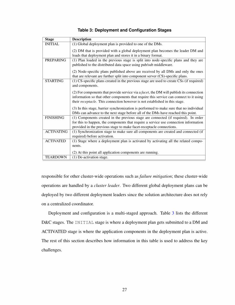
Table 3: Deployment and Configuration Stages
Stage DescriptionINITIAL (1) Global deployment plan is provided to one of the DMs.
(2) DM that is provided with a global deployment plan becomes the leader DM andloads that deployment plan and stores it in a binary format.
PREPARING (1) Plan loaded in the previous stage is split into node-specific plans and they arepublished to the distributed data space using pub/sub middleware.
(2) Node-specific plans published above are received by all DMs and only the onesthat are relevant are further split into component server (CS)-specific plans.
STARTING (1) CS-specific plans created in the previous stage are used to create CSs (if required)and components.
(2) For components that provide service via a facet, the DM will publish its connectioninformation so that other components that require this service can connect to it usingtheir receptacle. This connection however is not established in this stage.
(3) In this stage, barrier synchronization is performed to make sure that no individualDMs can advance to the next stage before all of the DMs have reached this point.
FINISHING (1) Components created in the previous stage are connected (if required). In orderfor this to happen, the components that require a service use connection informationprovided in the previous stage to make facet-receptacle connections.
ACTIVATING (1) Synchronization stage to make sure all components are created and connected (ifrequired) before activation.
ACTIVATED (1) Stage where a deployment plan is activated by activating all the related compo-nents.
(2) At this point all application components are running.TEARDOWN (1) De-activation stage.
responsible for other cluster-wide operations such as failure mitigation; these cluster-wide
operations are handled by a cluster leader. Two different global deployment plans can be
deployed by two different deployment leaders since the solution architecture does not rely
on a centralized coordinator.
Deployment and configuration is a multi-staged approach. Table 3 lists the different
D&C stages. The INITIAL stage is where a deployment plan gets submitted to a DM and
ACTIVATED stage is where the application components in the deployment plan is active.
The rest of this section describes how information in this table is used to address the key
challenges.
27

III.4.2 Addressing Resilient D&C Challenges
Resolving Challenge 1 (Distributed Group Membership): To support distributed group
membership, we require a mechanism that allows detection of joining members and leaving
members. To that end the solution presented uses a discovery mechanism to detect the
former and a failure detection mechanism to detect the latter as described below.
Discovery Mechanism: Since the solution approach relies on an underlying pub-
/sub middleware, the discovery of nodes joining the cluster leverages existing discov-
ery services provided by the pub/sub middleware. To that end we have used OpenDDS
(http://www.opendds.org) – an open source pub/sub middleware that implements OMG’s
Data Distribution Service (DDS) specification [70]. To be more specific, we use the Real-
Time Publish Subscribe (RTPS) peer-to-peer discovery mechanism specified by DDS.
Failure Detection Mechanism: To detect the loss of existing members, a failure de-
tection mechanism is required. In the solution architecture this functionality is provided
by the GMM. The GMM residing on each node uses a simple heartbeat-based protocol to
detect DM (process) failure. Recall that any node failure, including the ones caused due to
network failure, results in the failure of its DM. This means that the failure detection service
uses the same mechanism to detect all three different kinds of infrastructure failures.
Resolving Challenge 2 (Leader Election): Leader election is required in order to toler-
ate cluster leader failure. This is implemented using a rank-based leader election algorithm.
Each DM is assigned a unique numeric rank value and this information is published by each
DM as part of its heartbeat. Initially the DM with the least rank will be picked as the cluster
leader. If the cluster leader fails, each of the other DMs in the cluster will check their group
membership table and determine if it is the new leader. Since, a unique rank is associated
with each DM, only one DM will be elected as the new leader.
Resolving Challenge 3 (Proper Sequencing of Deployment): The solution D&C infras-
tructure implements deployment synchronization using a distributed barrier synchroniza-
tion algorithm. This mechanism is specifically used during the STARTING stage of the
28

D&C process to make sure that all DMs are in the STARTING stage before any of them
can advance to the FINISHING stage. This synchronization is performed to ensure that all
connection information of all the components that provide a service is published to the dis-
tributed data space before components that require a service try to establish a connection.
We realize that this might be too strong of a requirement and therefore we intend to further
relax this requirement by making sure that only components that require a service wait for
synchronization. In addition, the current solution also uses barrier synchronization in the
ACTIVATING stage to make sure all DMs advance to the ACTIVATED stage simultane-
ously. This particular synchronization ensures the simultaneous activation of a distributed
application.
Resolving Challenge 4 (D&C State Preservation): In the current implementation, once
a deployment plan is split into node-specific deployment plans, all of the DMs receive
the node-specific deployment plans. Although any further action on a node-specific de-
ployment plan is only taken by a DM if that plan belongs to the node in which the DM
is deployed, all DMs store each and every node-specific deployment plans in its memory.
This ensures that deployment-related information is replicated throughout a cluster thereby
preventing single point of failure. However, this approach is vulnerable to DM process
failures since deployment information is stored in memory. To resolve this issue, the solu-
tion presented in this section can be extended to use a persistent backend database to store
deployment information.
III.5 Experimental Results
This section demonstrates the autonomous resilience capabilities of the D&C infras-
tructure by showing how it adapts applications as well as itself after encountering a node
failure during deployment-time, and runtime.
29

III.5.1 Testbed
For all experiments, a cluster of three nodes was used. Each node had a 1.6 GHz Atom
N270 processor and 1GB of RAM. Each node ran vanilla Ubuntu 13.04 server image which
uses Linux kernel version 3.8.0-19.
The application that was used for the experiments presented in Sections III.5.2 and III.5.3
is a simple two-component client-server experiment presented earlier in Figure 7. The
Sender component (client) is initially deployed in node-1, the Receiver component (server)
is initially deployed in node-2, and node-3 has nothing deployed on it. For both exper-
iments, node-2 is the node that fails. Furthermore, the infrastructure is configured with
heartbeat period set to 2 seconds and failure monitoring period set to 5 seconds.
III.5.2 Node Failure During Deployment-time
Figure 9 presents a time sequence graph of how the D&C infrastructure adapts itself
to tolerate failures during deployment-time. As can be seen, node 2 and therefore DM-2
fails at Event 5. Once the failure is detected by both DM-1 in node-1 and DM-3 in node-3,
DM-1 being the leader initiates the recovery process (Event 6 - Event 7). During this time,
DM-1 determines the part of the application that was supposed to be deployed by DM-2
in node-2, which is the Receiver component. Once DM-1 determines this information,
it completes the recovery process by republishing information about the failure affected
part of application (Receiver component) to DM-3. Finally, DM-3 deploys the Receiver
component in node-3 and after this point, the deployment process resumes normally.
III.5.3 Node Failure During Application Run-time
Figure 10 presents a time sequence graph that demonstrates how the D&C infrastruc-
ture adapts applications at run-time to tolerate run-time node failures. Unlike the scenario
presented before where the initial deployment of the application has to be adapted to tol-
erate deployment-time failure, here the initial deployment completes successfully at Event
30

Figu
re9:
Dep
loym
entT
ime
Nod
eFa
ilure
.
31

Figu
re10
:R
untim
eN
ode
Failu
re.
32

19 after which the application is active. However, node-2 and therefore DM-2 fails at Event
20 and the notification of this failure is received by DM-1 at Event 21 after which DM-1
performs the recovery process similar to the way it did for deployment-time failure.
The one significant difference between the deployment-time failure mitigation and run-
time failure mitigation is that dynamic reconfiguration of application components is re-
quired to mitigate application run-time failure. To elaborate, once DM-3 deploys the Re-
ceiver component in node-3 it needs to publish new connection information for the Receiver
component allowing DM-1 to update Sender the component’s connection.
III.6 Related Work
Deployment and configuration of component-based software is a well-researched field
with existing works primarily focusing on D&C infrastructure for grid computing and Dis-
tributed Real-time Embedded (DRE) systems. Both DeployWare [35] and GoDIET [23] are
general-purpose deployment frameworks targeted towards deploying large-scale, hierarchi-
cally composed, Fractal [19] component model-based applications in a grid environment.
However, both of these deployment frameworks lack support for application reconfigura-
tion.
The Object Management Group (OMG) has standardized the Deployment and Configu-
ration (D&C) specification [77]. The Deployment And Configuration Engine (DAnCE)[82]
describes a concrete realization of the OMG D&C specification for the Lightweight CORBA
Component Model (LwCCM) [71]. LE-DAnCE [82] and F6 DeploymentManager [29]
are some of our other previous works that extend the OMG’s D&C specification. LE-
DAnCE deploys and configures components based on the Lightweight CORBA Component
Model [71] whereas the F6 Deployment Manager does the same for components based on
F6-COM component model [81]. The F6 Deployment Manager, in particular, focused on
the deployment of real-time component-based applications in highly dynamic DRE sys-
tems, such as fractionated spacecraft. However, similar to the work mentioned above,
33

these infrastructures also lack support for application adaptation and D&C infrastructure
resilience.
A significant amount of research exists in the field of dynamic reconfiguration of compo-
nent-based applications. In [11], the authors present a tool called Planit for deployment and
reconfiguration of component-based applications. Planit uses AI-based planner to come up
with application deployment plan for both - initial deployment, and subsequent dynamic re-
configurations. Planit is based on a sense-plan-act model for fault detection, diagnosis and
reconfiguration to recover from failures. Another work presented in [4], supports dynamic
reconfiguration of applications based on J2EE components. Although these solutions sup-
port application reconfiguration, none of them are themselves resilient.
The authors in [20] present the DEECo (Distributed Emergent Ensembles of Compo-
nents) component model, which is based on the concept of Ensemble-Based Component
System (EBCS). In general, this approach replaces traditional explicit component archi-
tecture by the composition of components into ensembles. An ensemble is an implicit,
inherently dynamic group of components where each component is an autonomic entity
facilitating self-adaptive and resilient operation. In [43], authors present a formal founda-
tion for ensemble modeling. However, they do not focus on the management infrastructure
required to deploy and reconfigure these components.
III.7 Concluding Remarks
This chapter presented a resilient Deployment and Configuration (D&C) infrastructure
(synonymous to a management infrastructure) for extensible CPS. Since extensible CPS
are dynamic and multi-tenant, a management infrastructure is required to manage lifecycle
of distributed applications (see Challenge 1 in Section I.3). Furthermore, since resilience is
of utmost importance for CPS in general, it is important for the management infrastructure
to be resilient. In addition, since extensible CPS are remotely deployed, resilience should
34

be autonomous. Although CPS are generally built using Component-Based Software Engi-
neering (CBSE) approach and there exists multiple component models with corresponding
D&C infrastructure, none of these existing D&C infrastructures can be considered resilient.
The work presented in this chapter incurs a few limitations: (1) As mentioned in Sec-
tion III.4.2, the current implementation for D&C state preservation is sufficient but not ideal
as deployment information should ideally be stored persistently to avoid DM process fail-
ure, (2) The D&C infrastructure presented in this chapter performs reconfiguration without
any smartness,i.e., we randomly decide where a component should be migrated. However,
this is not sufficient for systems that are dynamic and that can host multiple applications.
We require the D&C infrastructure to utilize available system information to make a more
educated decision on how a system should be reconfigured. This issue is addressed in the
solution presented in the next chapter (see Chapter V and Chapter VI).
III.8 Related Publications
1. Subhav Pradhan, Abhishek Dubey, and Aniruddha Gokhale. Designing a Resilient
Deployment and Reconfiguration Infrastructure for Remotely Managed Cyber-Physical
Systems. Lecture Notes in Computer Science (LNCS 2016), volume 9823. (To be
published)
2. Subhav Pradhan, Aniruddha Gokhale, William R. Otte, Gabor Karsai. Real-time
Fault Tolerant Deployment and Configuration Framework for Cyber Physical Sys-
tems. Proc. of the RTSS - WiP Session (RTSS-WiP 2012), pages 32 - 32, San Juan,
Puerto Rico.
3. Subhav Pradhan, William Otte, Abhishek Dubey, Csanad Szabo, Aniruddha Gokhale,
and Gabor Karsai. Towards a Self-adaptive Deployment and Configuration Infras-
tructure for Cyber-Physical Systems. Institute for Software Integrated Systems (ISIS)
Technical Report, ISIS-14-102, 2014, Nashville, TN, USA.
35

CHAPTER IV
ESTABLISHING SECURE INTERACTION ACROSS DISTRIBUTEDAPPLICATIONS
IV.1 Motivation
Consider the fractionated satellites cluster scenario presented as an example of exten-
sible CPS in Section V.1. One notable example for the use of the publish/subscribe pat-
tern in spacecraft software is NASA’s Core Flight Executive (CFE), which is a portable
platform-independent framework used as the basis for flight software for satellite data sys-
tems. The CFE uses publish/subscribe to facilitate communication between multiple ap-
plications. A review of the CFE revealed that the publish/subscribe style architecture not
only allowed distributed development and easy integration of applications but also allowed
applications to be encapsulated, which improved abstraction, flexibility, reuse and division
of concerns [34]. Thus, supporting this pattern in space systems is highly desirable.
Unfortunately, not all technologies that support publish/subscribe communication have
a comprehensive security model capable of partitioning information flows based on the
security classifications of applications. However, security is a key requirement for open
and distributed satellite clusters platforms since (1) space systems are extremely expensive
and therefore cannot afford security compromises with long term effects on the system, (2)
shared space systems are used by companies that are extremely sensitive about their data
and therefore require a strict security model.
In order to address this issue, this chapter presents a novel discovery mechanism that
ensures strict information partitioning by only allowing applications with compatible secu-
rity classification levels to discovery, and therefore, interact with each other. This ensures
strict information partitioning.
36

IV.2 Background and Problem Description
In order to better describe the problem at hand, this section first presents the system
model. Second, it presents an overview of OMG DDS including its discovery mechanism.
This is important since the middleware of choice for this work is OpenDDS [69], which is
an open source implementation of the OMG DDS specification. Third, this section presents
the problem statement in context of OpenDDS middleware.
IV.2.1 System Model
We consider each node of a satellite cluster to run a copy of the DistributedREaltime
Managed System (DREMS) platform [29, 33]. The only difference between DREMS ar-
chitecture and that presented in Section II.1, is that DREMS considers application compo-
nents to be hosted inside actors. Actors are the building blocks of this information system
and are similar to processes in traditional operating systems except that the Actor iden-
tifiers are unique across nodes and are not lost even after the death of the Actor. Actors
can be of two types: (1) Application Actors, and (2) Platform Actors. Application Actors
make up the mission-specific application functionality and can be dynamically installed
or removed. Platform Actors are actors related to platform services and they are part of
the Trusted Computing Base (TCB) [94, 95]. Applications hosted in our platform cannot
bypass the TCB and access resources, such as the network.
IV.2.2 OMG DDS Overview
The OMG Data Distribution Service (DDS) specification [72] defines a data-centric
communication standard for communication between DDS entities (data producers and
consumers) in a wide variety of environments. A DDS application consists of publishers
and subscribers, where publishers use data writers to produce data while subscribers use
data readers to consume data. The DDS specification also supports Quality of Service
37
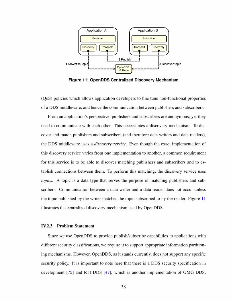
Figure 11: OpenDDS Centralized Discovery Mechanism
(QoS) policies which allows application developers to fine tune non-functional properties
of a DDS middleware, and hence the communication between publishers and subscribers.
From an application’s perspective, publishers and subscribers are anonymous; yet they
need to communicate with each other. This necessitates a discovery mechanism. To dis-
cover and match publishers and subscribers (and therefore data writers and data readers),
the DDS middleware uses a discovery service. Even though the exact implementation of
this discovery service varies from one implementation to another, a common requirement
for this service is to be able to discover matching publishers and subscribers and to es-
tablish connections between them. To perform this matching, the discovery service uses
topics. A topic is a data type that serves the purpose of matching publishers and sub-
scribers. Communication between a data writer and a data reader does not occur unless
the topic published by the writer matches the topic subscribed to by the reader. Figure 11
illustrates the centralized discovery mechanism used by OpenDDS.
IV.2.3 Problem Statement
Since we use OpenDDS to provide publish/subscribe capabilities to applications with
different security classifications, we require it to support appropriate information partition-
ing mechanisms. However, OpenDDS, as it stands currently, does not support any specific
security policy. It is important to note here that there is a DDS security specification in
development [75] and RTI DDS [47], which is another implementation of OMG DDS,
38

has recently implemented this specification. However this specification relies on the cor-
rect operation of the application and middleware to configure and enforce these policies.
Furthermore, relying on security model supported by the middleware itself requires us to
consider the entire middleware as part of the TCB [94, 95].
Figure 12: Topic based application interaction in OMG DDS
Existing DDS entities, such as topics and partitions cannot be used as mechanisms
to enforce information partitioning based on security labels since applications associated
with the same topic can have different security classifications. A naive solution would be to
create a topic for each security label, as shown in Figure 12. However, this approach has a
number of problems. First, it makes the applications responsible to subscribe to topics that
are appropriate to their security level. Second, this approach also relies on higher security
level applications to correctly refrain from publishing samples to topics to which lower
security level applications are subscribed to. Both these shortcomings are unworkable, as
we cannot trust applications to behave correctly.
IV.3 Solution Approach
This section presents the solution. To do so, this section first presents the target system
model as variance of the system model presented in Section II.1. Second, this section
39

presents brief description of the underlying Secure Transport (ST) mechanism1, since our
solution leverages capabilities of the ST. Finally, this section presents detailed description
of the novel discovery mechanism.
IV.3.1 Secure Transport
Secure Transport (ST) is a novel transport mechanism implemented in the OS kernel
that (1) restricts the communication pathways that can exist between any two processes
on the same computing node or on different computing nodes, (2) supports both unicast
as well as multicast transfers, (3) supports message authentication before transmission and
reception according to rules of a Multi-Level Security (MLS) policy [16, 29, 101], and (4)
provides packet level encryption for messages using IPSec 2.
MLS defines a policy based on partially ordered security labels that assign classifica-
tions and need-to-know categories to all information that may pass across process bound-
aries. This policy ensures that information is allowed to flow from a producer to a con-
sumer in DDS if and only if the label of the consumer is greater than or equal to that of
the producer. Both the allowed communication topology and the MLS policy labels must
be configured for each task by the secure discovery mechanism, which uses processes with
elevated system privileges to do so. By designing a solution that resides at the level of a
transport mechanism, we shield higher-level middleware, such as OMG DDS, from inva-
sive changes while at the same time providing them an opportunity to leverage these new
mechanisms.
Secure Transport (ST) comprises two key concepts: (1) endpoints, and (2) flows and
message transfer rules. These concepts are described below.
1Detailed description of ST mechanism is not part of this dissertation and can be found in [80].2The IPSec implementation in ST is the subject of ongoing work
40

IV.3.1.1 Endpoints
Endpoints are the basic communication resources used by applications to transmit and
receive messages; they are analogous to socket handles in the traditional BSD socket APIs.
Like traditional sockets, user space programs pass an endpoint identifier to the send and
receive system calls. Unlike traditional sockets, however, unprivileged tasks may not
arbitrarily construct endpoints that allow for inter-process communication with other tasks;
such endpoints must be explicitly configured by a privileged Actor that is part of a trusted
system configuration infrastructure. All endpoints are configured with a set of security
labels that can be used for sending messages through that endpoint.
Endpoints are separated into four different categories with different restrictions on their
creation and use; for the purposes of this discussion, we will describe only two endpoint
classes that are used for Inter-Process Communication (IPC):
• Local Message Endpoints (LME): Local message endpoints are the basic method
for IPC and may be used to send messages to other actors. These endpoints must
be configured by the trusted system configuration infrastructure and are subject to
restrictions placed by flows and security rules.
• Remote Message Endpoints (RME): Similar to LMEs, RMEs are a mechanism for
network IPC between Actors, but may be used to communicate with Actors hosted
by different operating system instances.
IV.3.1.2 Flows and Message Transfer Rules
Communication in ST is allowed between two LMEs or RMEs if and only if there
exist mutually compatible flows on each endpoint. A flow can be thought of as a logical
pipe between two endpoints and determines the direction in which messages can travel.
It provides system integrators the ability to specify the actors that are allowed to share
41

messages. The actual transfer of the message is further restricted by the MLS rules (see
below).
More concretely, a flow that is assigned to an endpoint is a connectionless association
with an endpoint owned by a designated Actor. This association determines if the local
endpoint is allowed to send or receive messages with the remote endpoint. Unicast flows
connect a source endpoint to a destination endpoint; multicast flows connect a source end-
point to multiple destination endpoints.
In all cases, the flow assignment between two endpoints must be mutual in order for
communication to succeed. Additionally, each message must be marked with the specific
label that indicates the security classification of that message. Message transmission is
allowed if and only if the following rules are satisfied. We refer the readers to [33] for a
full list of formal MLS rules.
• The label of the message must be within the label set of the sender endpoint.
• The sender must have an outbound flow to the recipient, and the recipient must have
a inbound flow from the sender.
• The receiver’s endpoints label must be either at the same classification level or at
a higher classification level of the received message. Thus, a lower classification
application cannot extract information from a higher classification application on the
reply path for a two-way communication because the labels on the return path do not
satisfy the MLS rules.
Performing message exchange via endpoints and flows enables decoupling between
senders and receivers, which operate only on their local endpoints without explicit knowl-
edge of the flows attached to those endpoints. For example, the flow connecting a client to
a failed server can be switched over to an alternative server transparently to the client.
42

IV.3.2 A Secure Discovery Mechanism
In order to describe the discovery mechanism in detail, we first need to understand
how the Deployment and Configuration (D&C) infrastructure in DREMS works because
it is responsible for assigning the security labels, setting up endpoints and the flows be-
tween communicating actors and ultimately playing a key role in the secure discovery. The
DREMS D&C is almost identical to the D&C infrastructure described in Chapter III. The
only difference is that the former extends the latter by adding aforementioned capabilities
related to the secure discovery mechanism.
IV.3.2.1 Overview of the D&C Infrastructure
The D&C infrastructure is responsible for the deployment and configuration of component-
based applications. Once an application is deployed, the D&C infrastructure is also respon-
sible for managing the application’s lifecycle throughout its lifetime. The D&C infrastruc-
ture is an implementation of the OMG D&C specification [78]3.
In a cluster there is exactly one Cluster Deployment Manager (CDM), which is respon-
sible for orchestrating the deployment and configuration (D&C) of applications across mul-
tiple nodes in the cluster. Each node has a single Node Deployment Manager (NDM) that
is responsible for taking node-specific actions. The CDM and NDM are Platform Actors
and are therefore considered to be part of the TCB. Finally, each node can have multiple
Component Servers (CS), which are spawned by NDMs as per requirement. All parts of
an application, i.e., component servers, components, and secure transport endpoints are
created by the D&C infrastructure according to a deployment plan, which is created by a
trusted system integrator. The trusted system integrator is also responsible for assigning
MLS labels to different applications.
3This is not the same as the D&C infrastructure presented previously in Chapter III
43

IV.3.2.2 An Architecture for Secure Discovery Mechanism
The discovery mechanism discussed in this section leverages existing discovery capa-
bilities provided by OpenDDS. OpenDDS supports two forms of discovery mechanisms:
(1) using a centralized information repository called the InfoRepo, and (2) using a peer-to-
peer approach where participating DDS applications discover each other in a collaborative
way rather than using a centralized information repository.
The peer-to-peer discovery approach requires all applications in a network be able to
communicate each other’s existence in order to perform discovery. This is not a workable
solution for our purpose as the communication restrictions enforced by ST mechanism
preclude any two unprivileged application processes spontaneously connecting with each
other. In addition, an application with lower security label must not be able to discover
the existence of other applications with a higher security label. Since we cannot use the
peer-to-peer discovery mechanism, our solution extends the centralized discovery service
provided by OpenDDS. Our extended capabilities require the following functionalities:
• The discovery mechanism should be able to establish Secure Transport information
flows between data writers and data readers of applications with matching security
labels. Since ST is a transport mechanism implemented in the kernel itself, it requires
the discovery mechanism to have elevated system privileges to create ST endpoints
and establish ST information flows.
• In addition to the discovery mechanism itself having system privileges, it should only
interact with other processes with system privileges. This prevents the centralized
repository from being a target of “data-at-rest” attacks.
• Normally, a discovery mechanism only checks for topic and relevant Quality of Ser-
vice (QoS) parameters when matching data writers and data readers. However, since
we are using the concept of security classification represented by security labels,
we require that the discovery mechanism also check these security labels during the
discovery process.
44

Table 4: Entities involved in the Secure Discovery Mechanism.
Entity FunctionalityDDS Entity This represents the various DDS related entities such as domain participants, data
writers and data readers. These entities are part of a user’s component-based ap-plications and therefore hosted inside their respective Component Servers (CSs).
DCPSInfo A singleton used to keep track of various DDS entities created by different appli-cations and inform the DDS middleware.
CS ORB This is the default CORBA Object Request Broker (ORB) [73] that is created whena CS is instantiated by a Node Deployment Manager (NDM). This ORB is usedby the CS to communicate with its parent NDM.
Discovery Callback All new data readers and data writers register a callback object, which is used bythe discovery mechanism to provide information regarding data reader/data writermatches.
DictM Proxy Since NDMs do not have access to the Dictionary Manager (DictM), this proxy isused for communicating with the DictM, which is collocated with the CDM.
Callback Proxy The Callback proxy is created by the DictM proxy. Upon creation of the Callbackproxy, the DictM proxy provides this information to the DictM. This is impor-tant because the DictM provides the data reader/data writers match information tothe Callback proxy, which in turn uses this information to establish the ST flowsbetween endpoints used by matching data readers and writers.The Callback proxy uses the ST interfaces to create these flows. Note that the STflows must be established before the DDS middleware can establish connectionbetween data readers and data writers by using their respective callback objects.
DM ORB This is the ORB used by the NDM and CDM to communicate with each other.DictM The Dictionary Manager (DictM) is a Platform Actor collocated with the CDM.
It acts as a central information repository, which is notified every time a new datareader or data writer is created. Upon creation of a new data writer, the DictMupdates information content and upon creation of a new data reader, the DictMfinds a matching writer (if any) and propagates this information to the callbackobjects of the created data readers.
To address these challenges and since we build on top of OpenDDS’ centralized ap-
proach, a centralized discovery mechanism called the Dictionary Manager (DictM) is used.
The DictM is a Platform Actor and therefore has system privileges to establish Secure
Transport information flows and it only interacts with other Platform Actors.
Figure 13 presents the architecture for the secure discovery mechanism showing how it
leverages the D&C infrastructure (and hence the TCB). Table 4 enlists the functionalities
of these entities. Figure 14 presents sequence diagrams illustrating (1) creation of a data
writer, and (2) association of a data reader with an existing data writer.
As shown in Figure 14, to create a data writer, first the Component Server creates a
DDS domain participant which in turn is used to create the data writer. Both the domain
45

Cluster Deployment Manager
DM ORB
DictM
Node Deployment Manager
DM ORB
DictM Proxy
Callback Proxy
Component Server
DCPSInfo
CS ORB
DDS Entity
Discovery Callback
Figure 13: Discovery Architecture. Table 4 describes the entities shown in thisfigure.
CreateDW_Proxy
DCPSInfoCSDomain
Participant
DataWriterCallback
DictMProxy
CallbackProxy
DictM
CreateDW_Callback
AddDW_Callback
Create DW
AddDW_Callback
AddDW_Proxy
Create Data Writer
DictMCallback
ProxyDataWriter
Callback
AddAssociation
AddAssociation
AssociationComplete
AssociationComplete
ConfigureSecureTransport
Data Reader Association
Figure 14: Sequence Diagram illustrating the process of (1) Data Writer Creation,and (2) Data Reader Association.
participant and data writer are DDS Entities. The domain participant also creates a data
writer callback, which is the Discovery Callback that will later be used to inform the data
writer about matching data readers. Once the data writer callback object is created, this
information is propagated to the DCPSInfo and DictM Proxy, which in turn creates a Call-
back Proxy and sends this information to be stored in the DictM.
Data reader creation follows the same pattern as that of a data writer. Once the data
reader is created and this information is propagated to the DictM, it finds the matching
data writer and adds the association. This process is also shown in Figure 14. Adding an
association consists of configuring a ST flow between endpoints of the matched data reader
46

and data writer. Once the ST flow is established, the association is complete and now the
DDS middleware can establish a connection between the data writer and the data reader.
IV.4 Experimental Evaluation
This section evaluates our solution in the context of a use case scenario. Since the
Secure Transport (ST) leverages IPv6, we also compare the effective performance of ST
against native IPv6; both transmitted over the same physical medium. This evaluation is
important since ST will be used for all the secure communication by our system and hence
the cost of using such a mechanism must be understood prior to its use.
IV.4.1 Experimental Setup
Figure 15 presents the setup of our experiment comprising two applications. These
applications use DDS for communication. Each application consists of a publisher and
subscriber. App-1 is hosted on node-1 and has security label unclassified, whereas, App-2
is hosted on node-2 and has the security label secret. App-2’s security label thus dominates
the label of App-1, and hence only App-1 is allowed to send information to App-2.
Publisher-1
Subscriber-1
Publisher-2
Subscriber-2
Node 1 Node 2
Topic-T
App-1 App-2 SecretUnclassified
Security label relation: Secret > Unclassified
Figure 15: Use case scenario: Two DDS Applications with Different Security Labels.
Based on the setup mentioned above, the subscriber in App-2 should be able to receive
messages published by publishers in both App-2 and App-1. However, the subscriber in
47

CONSUMER EVENT: Consumer_Message_data_listener_exec_i::on_one_data: received message <App1> Hello World. Test message from Provider <0>[LM_DEBUG] - 23:45:17.824504 - MessageDispatcher::execute_message - Message executed[LM_DEBUG] - 23:45:18.707008 - MessageDispatcher::execute_message - Deadline_type = DLT_NONE. Execute CMObject.CONSUMER EVENT: Consumer_Message_data_listener_exec_i::on_one_data: received message <App1> Hello World. Test message from Provider <1>[LM_DEBUG] - 23:45:18.708406 - MessageDispatcher::execute_message - Message executed[LM_DEBUG] - 23:45:19.707905 - MessageDispatcher::execute_message - Deadline_type = DLT_NONE. Execute CMObject.CONSUMER EVENT: Consumer_Message_data_listener_exec_i::on_one_data: received message <App1> Hello World. Test message from Provider <2>
Figure 16: App-1 Log Snippet which shows that App-1 only receives messagespublished by itself and not from App-2 since the latter has higher Security Label.
CONSUMER EVENT: Consumer_Message_data_listener_exec_i::on_one_data: received message <App2> Hello World. Test message from Provider <12>[LM_DEBUG] - 23:45:17.183886 - MessageDispatcher::execute_message - Message executed[LM_DEBUG] - 23:45:17.738411 - MessageDispatcher::execute_message - Deadline_type = DLT_NONE. Execute CMObject.CONSUMER EVENT: Consumer_Message_data_listener_exec_i::on_one_data: received message <App1> Hello World. Test message from Provider <0>[LM_DEBUG] - 23:45:17.739916 - MessageDispatcher::execute_message - Message executed[LM_DEBUG] - 23:45:18.180700 - MessageDispatcher::execute_message - Deadline_type = DLT_NONE. Execute CMObject.CONSUMER EVENT: Consumer_Message_data_listener_exec_i::on_one_data: received message <App2> Hello World. Test message from Provider <13>[LM_DEBUG] - 23:45:18.182083 - MessageDispatcher::execute_message - Message executed[LM_DEBUG] - 23:45:18.706913 - MessageDispatcher::execute_message - Deadline_type = DLT_NONE. Execute CMObject.CONSUMER EVENT: Consumer_Message_data_listener_exec_i::on_one_data: received message <App1> Hello World. Test message from Provider <1>[LM_DEBUG] - 23:45:18.708378 - MessageDispatcher::execute_message - Message executed[LM_DEBUG] - 23:45:19.180884 - MessageDispatcher::execute_message - Deadline_type = DLT_NONE. Execute CMObject.CONSUMER EVENT: Consumer_Message_data_listener_exec_i::on_one_data: received message <App2> Hello World. Test message from Provider <14>[LM_DEBUG] - 23:45:19.183357 - MessageDispatcher::execute_message - Message executed[LM_DEBUG] - 23:45:19.706862 - MessageDispatcher::execute_message - Deadline_type = DLT_NONE. Execute CMObject.CONSUMER EVENT: Consumer_Message_data_listener_exec_i::on_one_data: received message <App1> Hello World. Test message from Provider <2>
Figure 17: App-2 Log Snippet which shows that App-2 receives messages pub-lished by both itself and App-1 since it has higher Security Label than App-1.
App-1 should only be able to receive messages published by a publisher in App-1 since
App-2 is publishing messages with higher security label. To demonstrate this behavior,
Figures 16 and 17 present log message snippets4 captured during the execution of the
above-described use case with the appropriate App shown circled.
IV.4.2 Secure Transport Network Utilization
The Secure Transport (ST) mechanism presented previously in Section IV.3.1 is built
on top of IPv6. With any communication protocol, performance is a key concern, so the
effective performance (i.e., network utilization) of ST versus native IPv6 transmitted over
Ethernet was evaluated. First the overhead of the protocol and its average and maximum
4These log message snippets have been slightly modified in order to exclude irrelevant log messages.
48

throughput were calculated and compared to native IPv6. Since ST is built on top of IPV6,
each ST packet on the network incurs the same header overhead as an IPv6 packet.
Table 5: Network Utilization Calculations for IPv6 and for Secure Transport tunneledthrough an IPv4 network.
Message Utilization (8192B)IPV6 0.927956502
Minimum ST Header 0.924396299Average ST Header 0.921692169
Maximum ST Header 0.820348488
Additionally, each message includes a ST-specific header containing information about
the sending actor, the flow, the security labels, etc. This ST header is a minimum of 34 bytes
for the smallest security label, averages around 60 bytes for most security label lengths, and
has a maximum of 1,052 bytes for the longest security labels. Since a ST message can be
up to 8 Kilobytes and an Ethernet packet is at most 1500 bytes, only one transmitted packet
of each message will have the ST header. Since our test network on which we run IPv6 and
ST is a tunneled 6-to-4 network, we must add the IPv4 header length to our total packet
header. Finally, we choose UDP as our transport protocol for both IPv6 and the underlying
ST protocol, so UDP’s 8 byte header must be taken into account. The network utilization
calculations are presented in Table 5. These calculations are based on experiments executed
on a private testbed of nodes connected to each other through a gigabit Ethernet switch.
IV.5 Related Work
The OMG DDS specification, as currently specified, lacks an extensive security spec-
ification and therefore all DDS implementations lack a well-established security model.
However, RTI [47] and PrismTech [89] have combined their efforts to put forward a DDS
security proposal [75]. This proposal focuses on providing fine-grained, data-centric secu-
rity by providing (1) access control per DDS topic, (2) read/write permissions for related
49
DDS entities, and (3) field-specific permissions, which allow different fields of a particular
topic to have different permissions.
Even though this proposal is critical to the advancement of the state of the art in DDS,
however, a key issue that we have identified is that it relies on applications to correctly
configure the security policies required, and the middleware to correctly enforce them. This
requirement is fundamentally incompatible with a threat model where applications cannot
be trusted. Furthermore, unlike our approach, this proposal is directed towards a solution
that involves the entire DDS middleware to be part of the security model and therefore the
TCB. Since the TCB is assumed to be trusted, care should be taken to keep its size small.
Thus, maintaining the entire DDS middleware in the TCB is infeasible.
Similarly, prior efforts [14, 93] also require the entire DDS middleware to be part of the
TCB. In [93], the authors present an approach in which Authentication and Authorization
(AA) is embedded in the discovery mechanism which is implemented as a special network
application located within the DDS Real-time Pub/Sub (RTPS) layer. This approach differs
from ours since we place the centralized repository, used for discovery, outside of the DDS
middleware. The work presented in [14], focuses on integrating Role-based Access Control
(RBAC) with pub/sub communications. RBAC is similar to MLS in that the different roles
(security labels) provide principals (actors) with different services (access restrictions).
However, RBAC allows for the roles, in our case security labels, of a principal to change
during the lifetime of the application, something that we do not support as we consider
such flexibility as a potential source of attack.
[83] presents the notion of microguards for data access restrictions. Microguards are
distinct from the pub/sub middleware and are placed on domain boundaries to facilitate
information sanitization via transitioning policies between any two domains. The authors
argue that these microguards can be configured to perform checks that realize MLS poli-
cies. A limitation with guards is that they tend to be very specific to a data type and do not
support generic data communications. Also, in their network configuration, the guards sit
50

between networks or systems and connects them. They are not part of an actual system so
it is possible to use a different communication path to bypass the security enforced by these
guards. Such bypassing is not feasible in our solution. Furthermore, in our approach, all of
the MLS-related label checks are done by a single entity that provides the discovery service
rather than by distributing the task among multiple guards which introduces unnecessary
complications and leads to an increase in the number of possible points of attack.
The Component Information Flow (CIF) framework presented in [3] provides a way of
achieving data integrity and confidentiality during both intra- and inter-component commu-
nication. Labels are assigned to component ports at design-time via a policy file. However,
that work has some limitations with the type of systems considered here because it supports
label checking only at design and compile time.
IV.6 Concluding Remarks
This chapter presented a novel discovery mechanism that helps establish secure inter-
action between applications with varying security levels. This contribution is important
for extensible CPS, such as a satellite cluster, because of the open nature of these systems
in which applications from different vendors are likely to be simultaneously hosted on the
shared resource. As such, it is of utmost importance to devise a mechanism that facilitates
strict information partitioning between different applications to prevent data breaches by
ensuring only compatible applications entities can communicate with each other.
To that end this chapter presented (1) Secure Transport (ST), which is a transport mech-
anism that supports Multi-Label Security (MLS) labels and policies to represent and vali-
date security classifications, and (2) a secure discovery mechanism that is capable of estab-
lishing Secure Transport flows between DDS publish/subscribe applications with matching
security classifications. The use of a transport-level security mechanism ensures that no
invasive changes need to be made to the middleware. The results show that our system pro-
vides the necessary information partitioning and that the overhead of the ST is negligible.
51

IV.7 Related Publication
1. Subhav Pradhan, William Emfinger, Abhishek Dubey, William Otte, Daniel Balasub-
ramanian, Aniruddha Gokhale, Gabor Karsai, and Alessandro Coglio. Establishing
Secure Interactions Across Distributed Applications in Satellite Clusters. Proc. of
the 5th IEEE International Conference on Space Mission Challenges for Informa-
tion Technology (SMC-IT 2014), pages 67 - 74, Laurel, Maryland, USA.
52

CHAPTER V
ACHIEVING RESILIENCE IN EXTENSIBLE CPS VIASELF-RECONFIGURATION
V.1 Motivation
This chapter focuses on resilience of extensible CPS. Consider a mobile cyber-physical
platform of fractionated satellite, which is a cluster of independent satellite modules fly-
ing in formation and communicating with each other via ad-hoc wireless networks. Each
independent satellite that is part of a fractionated satellite cluster, can come from differ-
ent organization. This architecture can realize the functions of monolithic satellites at a
reduced cost and with improved adaptability and robustness [18]. Several existing and
future missions use this type of architecture, including NASA’s Edison Demonstration of
SmallSat Networks, TANDEM-X, PROBA-3, and PRISMA from Europe. In each of these
missions, the cooperating fractionated satellites are expected to provide the foundation for
applications running simultaneously using shared resources.
Each satellite modules of a fractionated satellite cluster are present in the Low Earth
Orbit (LEO), where one of the basic requirements is to be able to maintain orbital flight
so that they can overcome the atmospheric drag and orbit the Earth while remaining in the
LEO. Each individual satellite achieves this objective by periodically using their thrusters
to adjust their position. In addition to this critical objective, other objectives can be added
by hosting different applications. Figure 18 presents an overview of a fractionated satellite
cluster hosting two different component-based applications with mixed criticality. The
first application is a high-priority Cluster Flight Application (CFA), which is responsible
for maintaining flight control. The second application is lower priority Image Processing
Application (IPA), which is responsible for capturing and processing real-time images.
53

Figure 18: Distributed Deployment of Applications with mixed-criticality on a Frac-tionated Satellite Cluster.
As shown in Figure 18, the high-priority CFA application comprises four different com-
ponents. Next, we briefly describe the different functions provided by these components.
A schematic overview of the associated tasks performed by these components is presented
in Figure 19.
• ModuleProxy: This component behaves as an interface between different satellite
sensors and the OrbitMaintenance component, allowing the OrbitMaintenance com-
ponent to access available sensors.
• OrbitMaintenance: This component is responsible for tracking the state of a cluster
satellite. To perform this task, it uses the ModuleProxy component to acquire the
latest information, such as location co-ordinates. Once appropriate information is
collected, this component is also responsible for disseminating this information as
a packaged structure to all other satellites in the cluster. As every satellite runs an
instance of CFA, each node periodically receives updates from the other nodes.
• CommandProxy: This component performs the task of receiving commands from
a ground station. When a command is received, it sends the command to its local
54

M11 O1
1 O21
M12 O1
2 O22
M13 O1
3 O23
C11 T 1
1 T 21 M2
1
C12 T 1
2 T 22 M2
2
C13 T 1
3 T 23 M2
3
Task Component ActivityM1
ModuleProxyInform O1 of new state
M2 Activate engineO1
OrbitalMaintenancePublish new state
O2 Subscribe to new stateT 1
Tra jectoryPlanningPublish new command
T 2 Subscribe to new commandC1 CommandProxy Inform T 1 of command
Figure 19: Tasks performed by components of the Cluster Flight Application. Forthese tasks, the subscript represents the ID of the node onto which a task is de-ployed. The total latency of the interaction C1
1 → M2N represents the total latency
between receiving the scatter command and activating the thrusters. This interac-tion pathway is in bold.
TrajectoryPlanning component. Furthermore, commands received from a ground
station are also forwarded to other satellite nodes in a cluster.
• TrajectoryPlanning: This component is responsible for performing the task of re-
ceiving commands from the local CommandProxy component and responding to
those commands using satellite thrusters, if required, to perform highly critical, hard
real-time tasks.
The lower priority IPA is a comparatively simpler application. It comprises a compo-
nent that uses the camera to capture real-time images (sensing) and another component that
processes the captured images. These are periodic CPU-intensive tasks that are temporally
isolated [88] from each other. As mentioned before, the IPA is a lower priority application
when compared to the CFA. As such, the IPA tasks are executed by application threads that
have lower priority than that of the CFA.
Extensible CPS like the fractionated satellites host mission critical applications that
55

necessitate support for resilience mechanisms. In addition to hosting mission critical appli-
cations, platforms like fractionated satellites are remotely deployed and therefore require
autonomous resilience. Self-reconfiguration is one way to achieve autonomous resilience.
In addition to runtime self-reconfiguration mechanisms, design-time analysis and verifica-
tion are also important since they can be used to perform admittance checks on applica-
tions at design-time before they are deployed on the target system. It is important to find
errors and anomalies as quickly as possible since a small error at design-time, such as a
Quality-of-Service (QoS) requirement mismatch, can propagate and quickly affect other
applications, sub-systems, or an entire system.
V.2 Background and Problem Description
In order to describe the problem at hand, this section first presents a mechanism used to
describe extensible CPS. Then the resource and deployment models are presented. Finally,
this sections presents the problem statement.
V.2.1 Goal-based System Description
Extensible CPS are dynamic in nature and therefore require a generic way to represent
system goals expected to be satisfied by a system during a given time interval. A time
interval sequence consisting of high-level system objectives that must be available during
those intervals is called a mission goal. Different systems associated with a cyber-physical
platform are mission oriented and therefore have specific mission goals. Since objectives
are essentially functions, system objectives can be defined using the concept of functional
decomposition, which is the process of decomposing high-level functions into a set of sub-
functions, until a set of leaf-level functions is reached. Leaf-level functions are functions
that cannot be decomposed, and they are mapped to components [52, 61] that provide
these functions as services. Services are provided or required by components through their
56

Figure 20: Functional Decomposition Graph for a simple two-application System.
ports. This approach of goal-based system description is not novel as it has been previ-
ously presented in [24, 92]. However, the work presented in this chapter, as well as, the
next (see Chapter VI) uses the goal-based system description approach for management of
distributed applications.
Components are the basic unit of system composition. As shown in Figure 20, a com-
ponent can provide one or more functions (leaf-level or non leaf-level) via its ports. Fur-
thermore, different components can provide the same functionality. If a functionality is
provided by multiple components, then any of those component can be deployed; this al-
lows more flexibility. Similarly, a component can also require one or more functions via
its ports. This provided and required relations between components and functions allow us
to establish dependencies between components. In addition to functions, a component can
also require resources in order to be considered available. As such, we classify a compo-
nent’s requirement into functional requirements and resource requirements.
Figure 20 presents the functional decomposition graph of a simple two-application sys-
tem. As shown in the figure, function f is a high-level function that represents a system’s
objective. Function f can be decomposed into sub-functions f1 and f2. Sub-function f1
can be further decomposed into leaf-level functions f3 provided by component C3 and f4
57

provided by component C1. Similarly, sub-function f2 can be decomposed into leaf-level
function f5 provided by component C2.
Definition 1. A functional decomposition is a directed acyclic graph (DAG), FD=(F,DE),
where F is the set of functions, and DE = F × F is the set of dependency edges. The
functions with zero indegree are called functions while the others are called sub-functions.
Definition 2. A software component is a collection, C = (P,S,R), where P is a set of ports
associated with a component, S is a set of functions provided by a component, and R is a
set of requirements.
Definition 3. An application is a graph of components, G = (C,E), where E ⊆ C×C
represent the control/data flow dependencies between components. These dependencies
impose operational requirements on components. That is, unless specified otherwise, a
component requires all other components to which it is connected to be available.
V.2.2 Resource Model
The physical computing infrastructure provides computation and communication re-
sources. Computation resources correspond to hardware facilities required to execute com-
putation tasks at a given computation node. These include processing speed (number of
instructions per second), memory size (amount of memory required), and specific hardware
required for certain tasks such as sensing or signal processing. Communication resources
on the other hand correspond to facilities required for interaction between tasks execut-
ing on different computation nodes. This includes communication bandwidth, available
security measures such as encryption, etc.
The resource model represents the capabilities and evolution of resources that are used
to carry out a mission, as a function of control inputs (actions) applied to the resources. For
example, the resource specification for a network link would include capability specifica-
tions like the maximum data flow capacity of the link. It would also include the possible
discrete states of the link, such as whether it is in service or broken.
58

V.2.3 Deployment Model
Deployment means instantiating a set of components and mapping them to available
physical resources. Given a set of currently deployed and active applications and a set of
components included in the application, we can deduce the set of system functions that can
be supported.
Definition 4. A deployment D = (dV ) is a function that maps software structure SC, which
is a set of component instances and their inter-dependencies, to a hardware network HC =
(N,L), which is a DAG, where N is the set of nodes, and L = N → N is the set of links
between these nodes. A communication link resource function is a function N×L⇒N that
represents the capacity of a specific communication link on a node. dV : C→ N, where C
is a set of components.
V.2.3.1 Alternate Deployment Configurations
Two deployment configurations are considered to be alternatives if they deploy the
same set of applications on the same physical architecture within the same resource con-
straints while satisfying the same set of goals. Alternate deployment configurations could
be compared against each other on the basis of resource cost and performance.
V.2.3.2 Configuration Space and Configuration Points
The configuration space of a platform represents the state space of the platform. This
includes (1) goal-based system description of different systems hosted on the platform,
(2) resource requirements of different components that are part of the system description,
(3) nodes that comprises the platform and their corresponding resources, such as memory,
storage, and devices, and (4) deployment constraints that determine whether components
should be collocated on the same node, distributed across different nodes, or always de-
ployed on a specific node. A configuration space can expand or shrink depending upon
addition or removal of related entities.
59

A configuration space can contain multiple configuration points. A configuration point
represents valid configurations of all systems that are part of the associated configuration
space. A valid configuration of a system represents component to node mappings (de-
ployment) for all components that are required to satisfy the system’s goal. We always
begin with a valid configuration point, which we call the initial configuration point. Ini-
tial configuration point represents the initial deployment of different systems. Similarly,
current configuration point represents the current deployment. A configuration point, since
it is a component-to-node mapping, can be represented using a component-to-node matrix
defined below.
Definition 5 (C2N matrix). A C2N matrix comprises rows that represent component in-
stances and columns that represent nodes; the size of this matrix is α×β , where α is the
number of component instances and β is the number of available nodes (Equation V.1).
Each element of the matrix is encoded as a Z3 integer variable whose value can either be 0
or 1 (Equation V.2). A value of 0 for an element means that the corresponding component
instance (row) is not deployed on the corresponding node (column). Conversely, a value
of 1 for an element indicates deployment of the corresponding component instance on the
corresponding node. For a valid C2N matrix, a component instance must not be deployed
more than once (Equation V.3).
C2N =
c2n00 c2n01 c2n02 . . . c2n0β
c2n10 c2n11 c2n12 . . . c2n1β
c2n20 c2n21 c2n22 . . . c2n2β
. . . . . . . . . . . . . . . .
c2nα0 c2nα1 c2nα2 . . . c2nαβ
=
c2ncn : c ∈ {0 . . .α},n ∈ {0 . . .β},(α,β ) ∈ Z+ (V.1)
60

∀c2ncn ∈C2N : c2ncn ∈ {0,1} (V.2)
∀c :β
∑n=0
c2ncn <= 1 (V.3)
At any given point in time only one of the configuration point reflects the reality of
the deployed system; this is the current configuration point. All other configuration points
are implicitly present in the configuration space, but have to be computed dynamically at
runtime. This is precisely what happens when a failure is detected. When a failure occurs,
current configuration point is marked as faulty, specifically some component(s) or node(s)
are marked as faulty, rendering corresponding row (s) or column (s) of the the C2N ma-
trix with 0 markings and a constraint that it cannot be used in future unless the fault has
been removed. For example, consider a scenario where multiple configuration points maps
one or more components to a node. If this node fails, then all aforementioned configura-
tion points are rendered faulty. Given these concepts of configuration space and points,
recovering from failure essentially involves self-reconfiguration of the system by finding a
new valid configuration point and determining actions required to transition from current
(faulty) configuration point to the new (desired) configuration point. As such, configuration
points and their transitions form the very core of our self-reconfiguration mechanism.
For a more detailed description of a configuration space and its configuration points,
please refer to our previous work [85], which presents a feature model that we use to
represent a configuration space.
V.2.4 Problem Statement
Extensible CPS can host numerous mission critical cyber-physical applications. Each
application consists of components providing different functions to meet various objectives
and therefore the mission goal. As such, it is of utmost importance to make sure that all
61

functions and their corresponding components required to maintain a system’s goal are
preserved in the face of failures and anomalies. Therefore, for cyber-physical platforms,
such as the fractionated satellite cluster described as a motivating scenario in Section II.4,
resilience is a key requirement. We adopt the definition of resilience from [54]: “The
persistence of the avoidance of failures that are unacceptably frequent or severe, when
facing changes.” Although a truly resilient system needs to be resilient against failures,
changes (intended or unintended), and updates, this dissertation focus only on resilience
against failures.
We identify the following as requirements that need to be satisfied to achieve cyber-
physical platforms that are capable of supporting autonomous resilience:
Requirement 1 - Design-time analysis tools for admittance checking: Application re-
quirements, such as timing and network QoS requirements, and properties like resilience
should be analyzed and validated at design-time.
Requirement 2 - Runtime mechanism to facilitate autonomous resilience: We require
a distributed runtime mechanism capable of providing autonomous resilience. Any such
mechanism should be able to monitor, detect, diagnose, and mitigate failures.
There exists multiple solutions to satisfy Requirement 1 [32, 51]. As a minor contribu-
tion associated with Requirement 1, this chapter presents a novel design-time tool capable
of performing resilience analysis. Most of the work presented in this chapter focuses on
Requirement 2. There exists significant amount of research literature related to failure mon-
itoring, detection, diagnosis, and mitigation. Most of this can be leveraged for extensible
CPS, however, existing solutions for failure mitigation cannot be used as they do not take
into account the scale and the dynamic nature of these platforms. As such, the contribu-
tion of this chapter is a novel self-reconfiguration mechanism that facilitates autonomous
resilience.
62

V.3 Solution Approach
This section presents the solution in detail. First, an overview of the solution approach is
presented. Second, the design-time resilience analysis tool is presented. Third, the runtime
infrastructure for self-reconfiguration mechanism is presented.
V.3.1 Overview of the Solution Approach
An overview of our solution approach is shown in Figure 21; it comprises design-
time and runtime aspects. The design-time aspect of the solution includes a graphical
modeling tool developed using the Generic Modeling Environment (GME) [55], associated
model interpreters, a design-time resilience analysis tools (described in Section V.3.2), and
a database to store artifacts generated and analyzed by aforementioned interpreters and
analysis tools. The database is also part of the runtime aspect. We can view this database
as a medium through which relevant information is shared between entities of the design-
time and runtime entities. In addition to the database, the runtime aspect also includes a
management infrastructure, a managed system, a monitoring infrastructure, and a resilience
infrastructure. These runtime entities form an autonomous resilience loop akin to a sense-
plan-act loop, which is the basis of our approach to realizing a self-reconfiguring system.
Figure 21: Overview of the Solution Approach.
63

The monitoring infrastructure performs the task of sensing; it is responsible for mon-
itoring a managed system to detect and diagnose failures. The resilience infrastructure
performs the task of planning; it is responsible for covering the self-reconfiguration mech-
anism. Finally, the management infrastructure performs the task of acting; it is responsible
for undertaking actions computed (planned) by the resilience infrastructure. In our im-
plementation, which is described in detail in Section V.3.3, the monitoring infrastructure
comprises distributed monitors for failure detection, the resilience infrastructure comprises
a Satisfiability Modulo Theories (SMT) [15] based solver, and the management infrastruc-
ture comprises distributed Deployment Managers (DMs), where a single DM is deployed
on every node.
A typical workflow is as follows. The user begins by creating a model and defining
components, which provide the basic units of functionality. The definition of a component
includes its communication ports and timing requirements. Next, one or more applications
are created by assembling components together and configuring their communication. For
instance, the output port of one component may be connected to the input port of another
component. Based on applications that need to be deployed on the target platform, mission
goals (see Section V.2.1) are defined. At this point design-time analysis tools and model
interpreters are used to analyze the design-time model and generate appropriate artifacts
that represent a configuration space and initial configuration point (see Section V.2.3.2)
for the modeled system. These are stored in the database and is later used at runtime; the
initial configuration point is used for initial deployment and the configuration space is used
to compute new configuration points at runtime in order to reconfigure the system. We
describe this process in detail in Section V.3.3.2.
V.3.2 Design-time Resilience Analysis Tool
The section describes in detail a novel design-time resilience analysis tool. This tool
is useful in the context of extensible CPS for which resilience is of utmost importance. In
64
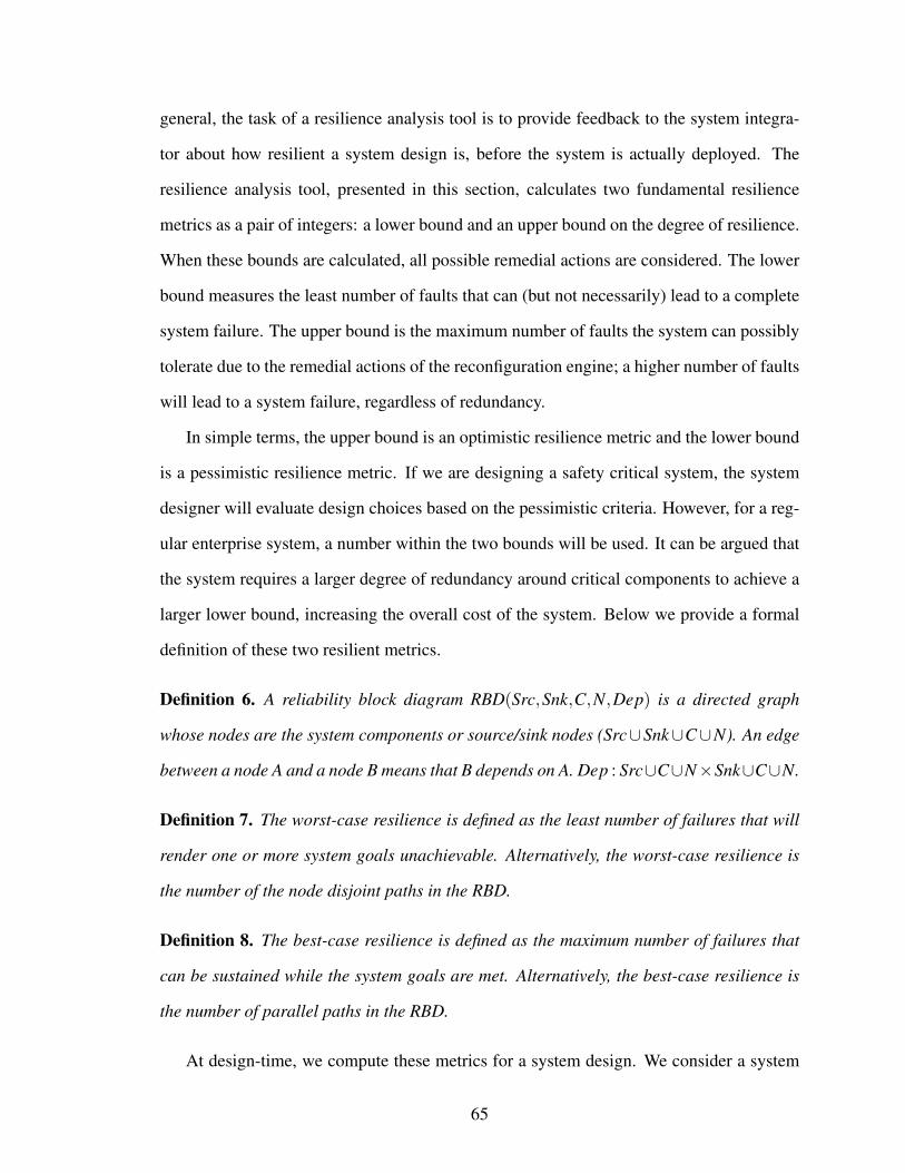
general, the task of a resilience analysis tool is to provide feedback to the system integra-
tor about how resilient a system design is, before the system is actually deployed. The
resilience analysis tool, presented in this section, calculates two fundamental resilience
metrics as a pair of integers: a lower bound and an upper bound on the degree of resilience.
When these bounds are calculated, all possible remedial actions are considered. The lower
bound measures the least number of faults that can (but not necessarily) lead to a complete
system failure. The upper bound is the maximum number of faults the system can possibly
tolerate due to the remedial actions of the reconfiguration engine; a higher number of faults
will lead to a system failure, regardless of redundancy.
In simple terms, the upper bound is an optimistic resilience metric and the lower bound
is a pessimistic resilience metric. If we are designing a safety critical system, the system
designer will evaluate design choices based on the pessimistic criteria. However, for a reg-
ular enterprise system, a number within the two bounds will be used. It can be argued that
the system requires a larger degree of redundancy around critical components to achieve a
larger lower bound, increasing the overall cost of the system. Below we provide a formal
definition of these two resilient metrics.
Definition 6. A reliability block diagram RBD(Src,Snk,C,N,Dep) is a directed graph
whose nodes are the system components or source/sink nodes (Src∪Snk∪C∪N). An edge
between a node A and a node B means that B depends on A. Dep : Src∪C∪N×Snk∪C∪N.
Definition 7. The worst-case resilience is defined as the least number of failures that will
render one or more system goals unachievable. Alternatively, the worst-case resilience is
the number of the node disjoint paths in the RBD.
Definition 8. The best-case resilience is defined as the maximum number of failures that
can be sustained while the system goals are met. Alternatively, the best-case resilience is
the number of parallel paths in the RBD.
At design-time, we compute these metrics for a system design. We consider a system
65

design as a pair: (1) an initial design i.e. the initial configuration point, and (2) the con-
figuration space. While the initial design describes the initial state of the system without
any failure, the configuration space implicitly describes all the feasible designs. If a pri-
mary fault causes secondary faults of other system entities, it is captured by the logical
constraints. For example, to enforce that the failure of a component brings down its host
process, we can add a constraint that enforces that. However, our current implementation
only considers node and component failures.
Primitive DescriptionAssign(i, j) Input: A component instance and a node.
Effect: A constraint that assigns component i to node jTurnToBinaryResource(c, n, c_list) Input: a component instance, a node, and a set of components that
are using the resource.Effect: a constraint that assigns component c to node n, and collo-cates all the client components present in c_list with c.
Enabled(i) Input: a component instance.Effect: a Boolean expression that is true if the component is as-signed to a node; false otherwise. The constraint sums the row ofthe component instance and checks if it is greater than zero.
CollocateComponents(c1, c2) Input: two component instances.Effect: a constraint that ensures that the component instances mustbe assigned to the same node.
DistributeComponents(c_list) Input: a list of component instances.Effect: a constraint that ensures that the component instances mustbe assigned to different nodes.
Communicates(i,j) Input: two component instances.Effect: a constraint that makes sure that there is a link between thenodes,the components are deployed on. If the,two components areon the same node, the constraint is still satisfied.
ForceExactly(f, c_list, n) Input: a function and a list of components; a positive integer n.Effect: a constraints that makes sure that exactly n of the compo-nents in the list must be enabled, to provide the function.
ForceAtleast(f, c_list, n) Input: a function and a list of components; a positive integer n.Effect: a constraints that makes sure that at least n of the compo-nents in the list must be enabled to provide the function.
ForceAtmost(f, c_list, n) Input: a function and a list of components; a positive integer n.Effect: a constraints that makes sure that at most n of the compo-nents in the list must be enabled to provide the function.
Table 6: Constraint Primitives implemented using Z3 Solver [26] Python APIs.
In order to perform resilience metrics computation, we formulate the problem as a SMT
problem, and use the Z3 solver [26] to solve the SMT problem. We describe the deployment
66

as an adjacency matrix (see Definition 5). The constraints are defined in Table 6. These
primitives are translated to equations over the adjacency matrix. For example, the primitive
Enabled and Assign are mapped as shown in Listing V.1. The Enabled function returns
true if a component with index i is assigned to any node. To do this it checks if the sum of
the row corresponding to that component is greater than 0. The Assign function ensures a
component is assigned to a particular node. The assignment is valid only if the component
is not in faulty state. Thus, the component being enabled implies the assignment, which
means that the element in the component’s row and the node’s column must be one. The
variable c2n represents the adjacency matrix in Z3, and Implies is the Python wrapper
around the implication in the Z3 library.
Listing V.1: Sample implementation of primitive constraints Enabled and Assign.# num_comp : Number o f components .# num_nodes : Number o f nodes .# c2n : A num_comp X num_nodes a d j a c e n c y mat r i x , where v a l u e s# are 0 or 1 . 0 meaning n o t e n a b l e d and 1 meaning e n a b l e d .# i : I n d e x o f a component t o e n a b l e .def Enabled ( s e l f , i ) :
re turn Sum ( [ s e l f . c2n [ i ] [ j ] f o r j in range ( s e l f . num_nodes ) ] ) > 0
# i : I n d e x o f a component t o e n a b l e .# j : I n d e x o f a node on which t h e component s h o u l d be e n a b l e ddef Ass ign ( s e l f , i , j ) :
re turn I m p l i e s ( s e l f . Enab led ( i ) , s e l f . c2n [ i ] [ j ] ==1)
Algorithm 1 Worst Case Metric Computation | Phase 1: Calling BFSINPUT: Adjacency Matrix and ConstraintsOUTPUT: Worst case metric
1: min = 02: for e 0 to |nodes
⋃components|−1 do
3: res = get_min_ f aults_b f s_r(0, [],e)4: if res == true then5: return
Once the components and the constraints have been generated, the solver is able to
compute solutions. As shown in Algorithm 1 and Algorithm 2, we find the worst case
resilience metric by performing a breadth-first search in the search space of injected faults.
67

We inject faults in the solver by specifying constraints, typically disabling one or more
components or nodes. The second phase of the algorithm is the recursive Breadth-First
Search (BFS). Essentially, we increase the number of faults each round in which we call
the BFS. The BFS combines together all the variations of faults, and when the level counter
reaches zero, the current state is evaluated by making all the components/nodes in the list
fail and checking if there is a solution. We save the solver state before this computation
(push) and restore it afterward on each control path (pop). Since the order is provided by a
BFS, whenever we cannot find a solution, we have found a minimal number of faults. This
is our worst case faults.
Algorithm 2 Worst Case Metric Computation | Phase 2: BFS Traversal |get_min_ f aults_b f s_rINPUT: start, list, levelOUTPUT: Worst case metric
1: if level == 0 then2: solver.push()3: for each element e in list do4: fail e5: solver.check()6: if no solution then7: save min as metric8: solver.pop()9: return true
10: solver.pop()11: return false12: for e in range of start and |nodes
⋃components|−1 do
13: res = get_min_ f aults_b f s_r(n+1, list +[e], level−1)14: if res == true then15: return true16: return false
The computation of the best-case metric is rather indirect. Instead of finding the max-
imum number of faults, we find a minimal configuration, and then subtract its number of
elements from the maximum number of elements in the initial model. This makes our com-
putation much more efficient because we can phrase this problem as a set of constraints for
Z3. We express the number of nodes and components as an integer variable n for the solver,
68
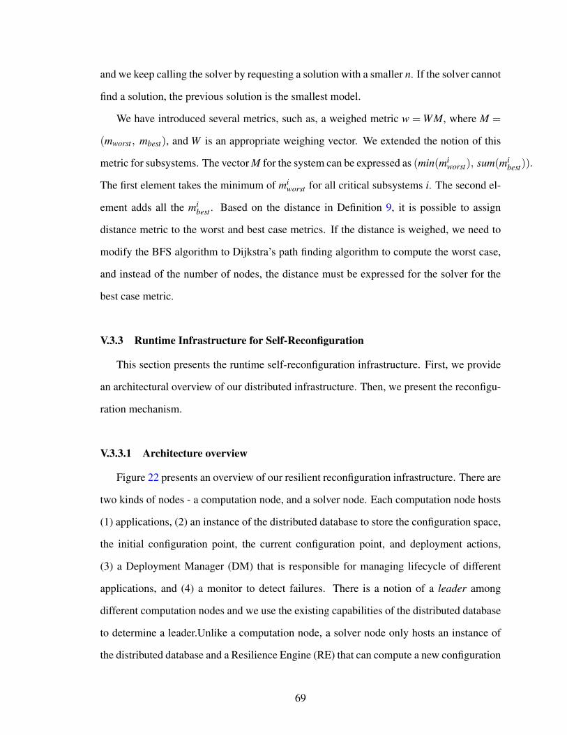
and we keep calling the solver by requesting a solution with a smaller n. If the solver cannot
find a solution, the previous solution is the smallest model.
We have introduced several metrics, such as, a weighed metric w = WM, where M =
(mworst , mbest), and W is an appropriate weighing vector. We extended the notion of this
metric for subsystems. The vector M for the system can be expressed as (min(miworst), sum(mi
best)).
The first element takes the minimum of miworst for all critical subsystems i. The second el-
ement adds all the mibest . Based on the distance in Definition 9, it is possible to assign
distance metric to the worst and best case metrics. If the distance is weighed, we need to
modify the BFS algorithm to Dijkstra’s path finding algorithm to compute the worst case,
and instead of the number of nodes, the distance must be expressed for the solver for the
best case metric.
V.3.3 Runtime Infrastructure for Self-Reconfiguration
This section presents the runtime self-reconfiguration infrastructure. First, we provide
an architectural overview of our distributed infrastructure. Then, we present the reconfigu-
ration mechanism.
V.3.3.1 Architecture overview
Figure 22 presents an overview of our resilient reconfiguration infrastructure. There are
two kinds of nodes - a computation node, and a solver node. Each computation node hosts
(1) applications, (2) an instance of the distributed database to store the configuration space,
the initial configuration point, the current configuration point, and deployment actions,
(3) a Deployment Manager (DM) that is responsible for managing lifecycle of different
applications, and (4) a monitor to detect failures. There is a notion of a leader among
different computation nodes and we use the existing capabilities of the distributed database
to determine a leader.Unlike a computation node, a solver node only hosts an instance of
the distributed database and a Resilience Engine (RE) that can compute a new configuration
69

Figure 22: Overview of the distributed self-reconfiguration infrastructure with De-ployment and Reconfiguration action sequences. Initial deployment is triggeredwhen a user/system integrator generates and stores the configuration space andthe initial configuration point for a system using the design-time modeling tool.Once this is done, a Resilience Engine (RE) is invoked to instigate initial deploy-ment. The RE then computes the required deployment actions and stores them inthe database. At this point, the Deployment Managers (DMs) that are responsiblefor taking these actions are notified after which they execute those commands lo-cally to complete initial deployment. Reconfiguration is similar, however, unlike auser/system integrator instigating the process, it is a monitor that instigates theprocess by logging information about any detected failure to the database and in-voking the RE. This should only be done by a single monitor, as such we dedicatethis task to the leader monitor, i.e., the monitor running on the leader node.
point when a system needs to migrate from one configuration point to another to mitigate
failures. Further descriptions of these are provided below.
Applications: As mentioned in section II.1, we assume component-based applications.
Therefore, each application is a set of components that interact with each other or with
components of different applications. All information required to deploy and configure
these applications on the target system is stored in a distributed persistent backend.
Distributed Database: A distributed database is required to store relevant information
such as (1) the configuration space, (2) the current configuration point, and (3) the initial
70

configuration point. The initial configuration point is provided by a system architect and is
used as the baseline for further reconfiguration when required. Well known faults are also
stored in the database as part of the configuration space. We use MongoDB [66] as our
choice of database and deploy multiple instances of this in a replica set.
Monitor: A monitor is responsible for monitoring, detecting and diagnosing failures.
This is an important aspect of a resilient system. However, there exists significant amount
of existing work in this particular research area, including works published by my collab-
orators in [30, 62]. As such, the work presented in this chapter does not focus on failure
monitoring, detection and diagnosis. For our experiments presented in Section VI.4, we
simply inject failures by updating system configuration stored in the database. In essence,
monitors in our architecture, as shown in Figure 22, are responsible for reporting diagnosed
failures to the database and invoking the Resilience Engine (RE) in order to initiate system
reconfiguration.
Resilience Engine: A Resilience Engine (RE) is primarily responsible for computing a
new configuration point at runtime when faults occur in the current state. This is important
because once a new configuration point is computed, reconfiguring the system involves
moving the system from the current configuration point, which is considered faulty, to the
new configuration point. The mechanism used to calculate a new configuration point is
described in Section V.3.3.2. In general, a RE first determines different entities affected by
the failure, and then it uses the Z3 solver to compute a new configuration point, considering
various constraints and available resources. If a new configuration point is successfully
computed, the local database instance is updated accordingly. This updated information is
later used by appropriate DMs to reconfigure the system.
Deployment Manager: In our architecture, Deployment Managers (DMs) running on
each node are used as local adaptation engines that are responsible for managing the life-
cycle of application components deployed on its node. Therefore, collectively, these DMs
71

form a distributed deployment and configuration infrastructure that manages various dis-
tributed applications by performing (1) initial deployment and configuration, (2) runtime
adaptation via reconfiguration, and (3) termination. In previous chapter (see Chapter III),
we identified key requirements for resilient deployment and configuration infrastructure
and implemented a prototype. Here we address the same requirements but our implemen-
tation is different and relies heavily on capabilities already provided by the distributed
database. For example, dynamic group membership is one of the key requirements identi-
fied and implemented in Chapter III (see Section III.4.1). However, for the work presented
in this chapter, we simply make use of group membership capability (i.e., replica set) sup-
ported by MongoDB.
As shown in Figure 22, DMs in our architecture simply listen for notification from their
local database instance. Although MongoDB does not include notification service, we
implement a simple notification mechanism based on MongoDB replica set Oplog, which
is a database collection that stores every database event. Once a DM is notified of an event
of its interest, it queries the database to obtain a set of application management actions
that it should perform. These actions will be related to application components hosted
on locally on the same node; a DM in one node cannot manage application components
deployed on a different node. Once a DM takes required actions, it updates the database
accordingly.
V.3.3.2 Reconfiguration
Once a failure is detected, our two-phase resilient recovery mechanism outlined in algo-
rithms 3 and 4 ensures that the system undergoes the required reconfiguration. The different
actions involved in this mechanism are also illustrated in Figure 22.
Phase 1 | Computing a new configuration point: The first phase of the reconfiguration
mechanism is instigated once a RE is invoked after detection of a failure. In this phase,
the RE computes a new configuration point by using information about the failure, the
72
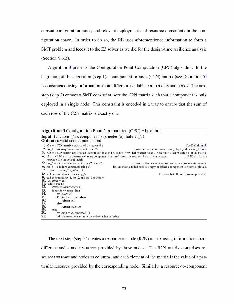
current configuration point, and relevant deployment and resource constraints in the con-
figuration space. In order to do so, the RE uses aforementioned information to form a
SMT problem and feeds it to the Z3 solver as we did for the design-time resilience analysis
(Section V.3.2).
Algorithm 3 presents the Configuration Point Computation (CPC) algorithm. In the
beginning of this algorithm (step 1), a component-to-node (C2N) matrix (see Definition 5)
is constructed using information about different available components and nodes. The next
step (step 2) creates a SMT constraint over the C2N matrix such that a component is only
deployed in a single node. This constraint is encoded in a way to ensure that the sum of
each row of the C2N matrix is exactly one.
Algorithm 3 Configuration Point Computation (CPC) Algorithm.Input: functions ( f n), components (c), nodes (n), failure ( f l)Output: a valid configuration point1: c2n = a C2N matrix constructed using c and n . See Definition 5.2: cst_1 = an assignment constraint over c2n . Ensures that a component is only deployed in a single node3: r2n = a R2N matrix constructed using nodes in n and resources provided by each node . R2N matrix is a resource-to-node matrix.4: r2c = a R2C matrix constructed using components in c and resources required by each component . R2C matrix is a
resource-to-component matrix.5: cst_2 = a resource constraint over r2n and r2c . Ensures that resource requirements of components are met.6: cst_3 = a failure constraint using f l . Ensures that a failed node is empty or failed a component is not re-deployed.7: solver = create_Z3_solver ()8: add constraint to solver using f n . Ensures that all functions are provided.9: add constraint cst_1, cst_2, and cst_3 to solver10: solution = null11: while true do12: result = solver.check ()13: if result == unsat then14: solver.pop()15: if solution == null then16: return null17: else18: return solution19: else20: solution = solver.model ()21: add distance constraint to the solver using solution
The next step (step 3) creates a resource-to-node (R2N) matrix using information about
different nodes and resources provided by those nodes. The R2N matrix comprises re-
sources as rows and nodes as columns, and each element of the matrix is the value of a par-
ticular resource provided by the corresponding node. Similarly, a resource-to-component
73

(R2C) matrix is created in the next step (step 4) using information about different compo-
nents and resources required by those components. The R2C matrix comprises resources
as rows and components as columns, and each element of the matrix is the value of a par-
ticular resource required by the corresponding component. The next step (step 5) of this
algorithm is to create a resource constraint using the aforementioned R2N and R2C matri-
ces. This constraint ensures that the resources required by components deployed on a node
is satisfiable.
Once the assignment and resource constraints are encoded, the next step (step 6) in Al-
gorithm 3 is to encode a failure constraint related to the failure that was initially detected.
If the failure was a node failure, we encode the constraint such that no components are de-
ployed on the failed node. Whereas, if the failure was a component failure, then we encode
the constraint such that the component is not re-deployed. The failure constraint related to
component failure could be relaxed by ensuring that a component gets re-deployed but not
on nodes where it has previously failed. At this point, all constraints are encoded and the
next few steps (steps 7 - 9) involves creating a Z3 solver and adding different constraints to
the solver.
Definition 9 (Least Distance Constraint). The “least distance” constraint is used to ensure
that we find a valid configuration point that is closest to the current configuration point.
The distance between two configuration points is the distance between their corresponding
C2N matrices. This distance is computed as shown in Equation V.4; the distance between
two valid configuration points A and B is the sum of the absolute difference between each
element of the C2N matrices corresponding to the two configuration points.
con f ig_distance =β
∑n=0|c2n_Acn− c2n_Bcn| (V.4)
After adding constraints to the solver, the next set of steps (steps 10 - 21) is responsible
for computing a configuration point that is the least distance (see Definition 9) away from
74

the current configuration point. In order to do so, we use a recursive logic, which upon
every successful solution computation (step 20) adds a distance constraint (step 21) and
invokes the solver again. The distance constraint is encoded using distance between com-
puted solution and the current configuration point. It is encoded to ensure a new solution
(one that will be computed in the next round of iteration) is lesser distance away from the
current configuration point in comparison to the solution computed in this iteration. As
such, by adding this constraint, we are asking the solver to find a better solution in ev-
ery iteration of successful solution computation. There will come a point when the solver
will not be able to find a better solution (step 13), in which case we check if the solution
from previous step is valid (step 15) and return that as the closest configuration point (step
18). This is an important heuristic as we do not want the system to deviate too much from
its current configuration. It also guarantees minimal reconfiguration time as the number of
changes required will be minimal due to the fact that the distance between the configuration
points is the least possible.
Once a new configuration point is computed, it is stored in the database as a desired
state. The next phase of our self-reconfiguration mechanism is responsible for using this
configuration point to compute reconfiguration commands required to transition from the
current configuration point to the new configuration point; we discuss this is detail be-
low. Here, it is important to note that our current implementation of the runtime self-
reconfiguration mechanism does not analyze or verify different properties (timing, network
QoS) of the configuration points computed at runtime. As mentioned before, this is an
important processes, specially for extensible CPS that host mission critical applications.
However, our work presented in chapter demonstrates our initial effort towards achieving
autonomous resilience; integrating analysis and verification of different properties with the
runtime reconfiguration loop is part of our future work.
Phase 2 | Computing reconfiguration commands and reconfiguring the system using
75

those commands: The second phase of our reconfiguration mechanism, shown in algo-
rithm 4, is responsible for computing reconfiguration commands and performing the recon-
figuration itself. In order to compute the reconfiguration commands required to transition
from one configuration point to another, the compute reconfiguration commands procedure
of Algorithm 4 is used. As shown, this procedure takes C2N matrices of newly computed
configuration point (step 3) and current configuration point (line 4) to determine different
reconfiguration commands (steps 5 - 13). To determine reconfiguration commands, we
check how each element of the aforementioned matrices are different when compared to
each other (steps 7 and 10). Depending on the difference we either create a start command
or a stop command. The former results in creation of a new process, whereas, the latter
results in termination of an existing process.
Algorithm 4 Reconfiguration Commands Computation and Reconfiguration Execution Al-gorithm.1: procedure COMPUTE RECONFIGURATION COMMANDS . Executed by the RE that computes a new configuration point.2: commands = null3: c2n_new = C2N matrix of the new configuration point . This is computed using Algorithm 34: c2n_cur = C2N matrix of the current configuration point5: for component c in c2n_new do6: for node n in c2n_new do7: if c2n_currcn < c2n_newcn then . Component missing in current8: create start command for component c in node n9: add command to commands list10: if c2n_currcn > c2n_newcn then . Component missing in new11: create stop command for component c in node n12: add command to commands list13: store commands in the database14:15: procedure RECONFIGURATION EXECUTION . Runs infinitely in each DM.16: if reconfiguration notification received then . One per command.17: retrieve the recon f iguration_command from the database18: if recon f iguration_command is for this node then19: if recon f iguration_command == START then20: create a new process and save pid in the database21: if recon f iguration_command == STOP then22: use component name to retrieve pid from the database23: kill the process using pid24: mark recon f iguration_command as executed in the database
Once all reconfiguration commands are computed and stored in the database, the recon-
figuration execution procedure of Algorithm 4 is used to ensure all reconfiguration com-
mands are executed. This procedure is executed infinitely by each DM.
76
When a DM is notified about a reconfiguration command (step 16), it checks if it should
execute that command (step 17). A DM should only execute commands that are targeted
for its host node. Once a DM determines a command that it should execute, it will check
whether the command is a start or stop command and execute the command accordingly
(steps 19 - 23). Finally, after executing a command, the DM updates the database to ac-
knowledge that the command has been executed. Once this happens for all reconfiguration
commands pertaining to a configuration point transition, we can claim that the system has
successfully self-reconfigured.
V.4 Case Study: Fractionated Satellite Cluster
In this section, we first present our use case scenario comprising three applications
deployed on a cluster of fractionated satellite. Second, we demonstrate the design-time
resilience metrics computation. Finally, we demonstrate the runtime self-reconfiguration
mechanism using a small scale system, and evaluate it using a larger system.
V.4.1 Scenario
In order to perform different demonstrations and evaluation, we use a fractionated satel-
lite scenario where we have a simple system with the following objectives: (1) satellite
flight applications to control the position of each satellite, (2) an imaging application to
capture images, and (3) a cluster flight planning application to coordinate the flight paths
and positions of the different satellites. The software (application) model for this system
is shown in Figure 23. We use a GME [55] based modeling front-end that allows a user to
model complex systems using a graphical modeling language.
As shown in Figure 23, this system is comprised of three different kinds of applica-
tions: (1) a single instance ofClusterFlightApplication, which is responsible for satisfying
the objective of coordinated flight planning, (2) three different instances of a flight control
77

Figure 23: Software Model Design using GME [55] based Modeling Language.
application called SatelliteFlightApplication, one for each node for a three-node initial de-
ployment scenario, and (3) a single instance of WAMApplication, which is responsible for
satisfying the imaging objective. The HardwareConfigurations for this application suggest
the requirements for the three nodes, which are named SatAlpha, SatBeta, and SatGamma
in the model. The initial deployment maps the ClusterFlightApplication to node SatAlpha,
the SatelliteFlightApplication instances to all three nodes, and three different components
of the WAMApplication to the three different nodes.
Each instance of the SatelliteFlightApplication is composed of three components (1)
an OrbitController component, which is responsible for manipulating thrusters to control
satellite movement and position, (2) a GroundInterface component, which is responsible
for communicating with a ground station, and (3) a SatelliteBusInterface component, which
is responsible for interacting with the satellite bus. The ClusterFlightApplication contains a
single component, a TrajectoryPlanner component, which is responsible for planning and
co-ordinating flights paths of the different satellites. The WAMApplication is composed
a HighResolutionImageGrabber component, a LowResolutionImageGrabber component,
78

and a ImageProcessor component; the first two components are responsible for captur-
ing images of varying resolution while the third component is responsible for processing
different images.
Not shown in Figure 23 are the different devices present on each node. For our scenario,
all three nodes host a BusController device to control the satellite bus and a GroundInter-
face device to communicate with a ground station. In addition, node SatAlpha also hosts
an HR_Camera device to capture high resolution images, an LR_Camera device to capture
low resolution images, and a GPU device to process captured images. Similarly, node Sat-
Beta also hosts a GPU device, and node SatGamma also hosts an HR_CAMERA device.
In addition to representing the system configuration after the initial deployment, Figure 24
also shows all these different devices with respect to their hosting nodes.
V.4.2 Resilience Metrics Calculation
Our current implementation of the design-time resilience analysis tool only considers
software component (application) failures and node failures. As such, the resulting re-
silience metrics are true only for component failures and node failures. In other words,
the minimum and maximum number of failures tolerable are strictly component failures or
node failures. Resilience analysis of system configuration presented in Figure 24 results
in resilience metrics of (1,12), where 1 is the worst-case metric and 12 is the best-case
metric. This means that the system is capable of tolerating at least one failure, regardless of
what the failure is, and at most twelve failures. Again, these failures are either component
or node failures. The thirteenth failure, regardless of which node or component it is, will
definitely cause the system to fail.
To further explain the computed resilience metrics, let us examine the worst-case met-
ric. Since the worst-case metric of 1 tells us that the system is always capable of tolerating
a single failure, let us come up with a scenario where two failures result in the system to be
non recoverable. If node SatGamma fails followed by the failure of node SatAlpha, we lose
79

Figu
re24
:S
yste
mC
onfig
urat
ion
afte
rIn
itial
Dep
loym
ento
fMod
elin
Figu
re23
.
80

both image capturing components of which at least one is required by the ImageProcessor
component on node SatBeta. Therefore, in this scenario, the two node failures was enough
to render the system non recoverable.
Similarly, we can evaluate the best-case metric by coming up with one or more sce-
narios that shows how the system can tolerate twelve failures. One such scenario is as
follows - (1) failure of the GroundInterface component on node SatGamma, which has no
effect as there are two other GroundInterface components, (2) failure of the GroundInter-
face component on node SatAlpha, which doesn’t require instantiation of the component
on another node but it does result in the TrajectoryPlanner component being restarted on
node SatBeta since this node has a functioning GroundInterface component to receive im-
portant commands from ground station, (3) failure of the HighResolutionImageGrabber
component on node SatGamma, which results in this component being restarted on node
SatAlpha, (4) failure of the SatelliteBusInterface on node SatGamma, (5) failure of the
OrbitController component on node SatGamma, (6) failure of node SatGamma itself, (7)
failure of the TrajectoryPlanning component on node SatBeta resulting in it being restarted
on node SatAlpha, (8) failure of the ImageProcessor component on node SatBeta resulting
in it being restarted on node SatAlpha, (9) failure of the LowResolutionImageGrabber on
node SatAlpha, which has no affect as the ImageProcessing component only requires one
out of two image capturing components, (10) failure of the GroundInterface on node Sat-
Beta, which results in system still being functional but not able to receive any new ground
commands, (11) failure of the SatelliteBusInterface component on node SatBeta, and fi-
nally (12) failure of the entire node SatBeta, which results in all remaining components
being hosted on node SatAlpha.
The purpose of computing these resilient metrics is to quantify the resilience of a sys-
tem. Using these metrics we can compare between different deployments or versions (for
example, with different resources) of the same system and determine the most resilient.
81

(a) Resilience metrics for different system models. (b) Resilience metrics computation time for differentsystem models.
Figure 25: Resilience Metrics (left) and corresponding computation time (right) fordifferent variation of system model presented in Figure 23. A represents the defaultmodel (shown in Figure 23), B represents a model in which a GPU device is removedfrom SatAlpha, C represents a model in which a HR_Camera is added to SatBeta,D represents a model in which a new node similar to SatGamma is added to thesystem, and E represents a model in which a new node similar to SatAlpha is addedto the system.
Based on this analysis, we can judge the tradeoffs between resilience and the different
system designs, and make a well-informed decision before deploying a system.
Figure 25 presents resilience metrics (Figure 25a) and corresponding computation time
(Figure 25b) for different variations of system model presented in Figure 23. As shown in
the figure, maximum failure computation time ranges between 20 - 30 seconds. Similarly,
minimum failure computation time ranges between 0 - 20 seconds for system models A
- D. However, minimum computation time for system model E is considerably higher at
126.63 seconds. This is because when a new node with five different devices is added to the
default model, the search space expands considerably for each failure scenario considered.
However, this is acceptable as this analysis is done during design-time.
82
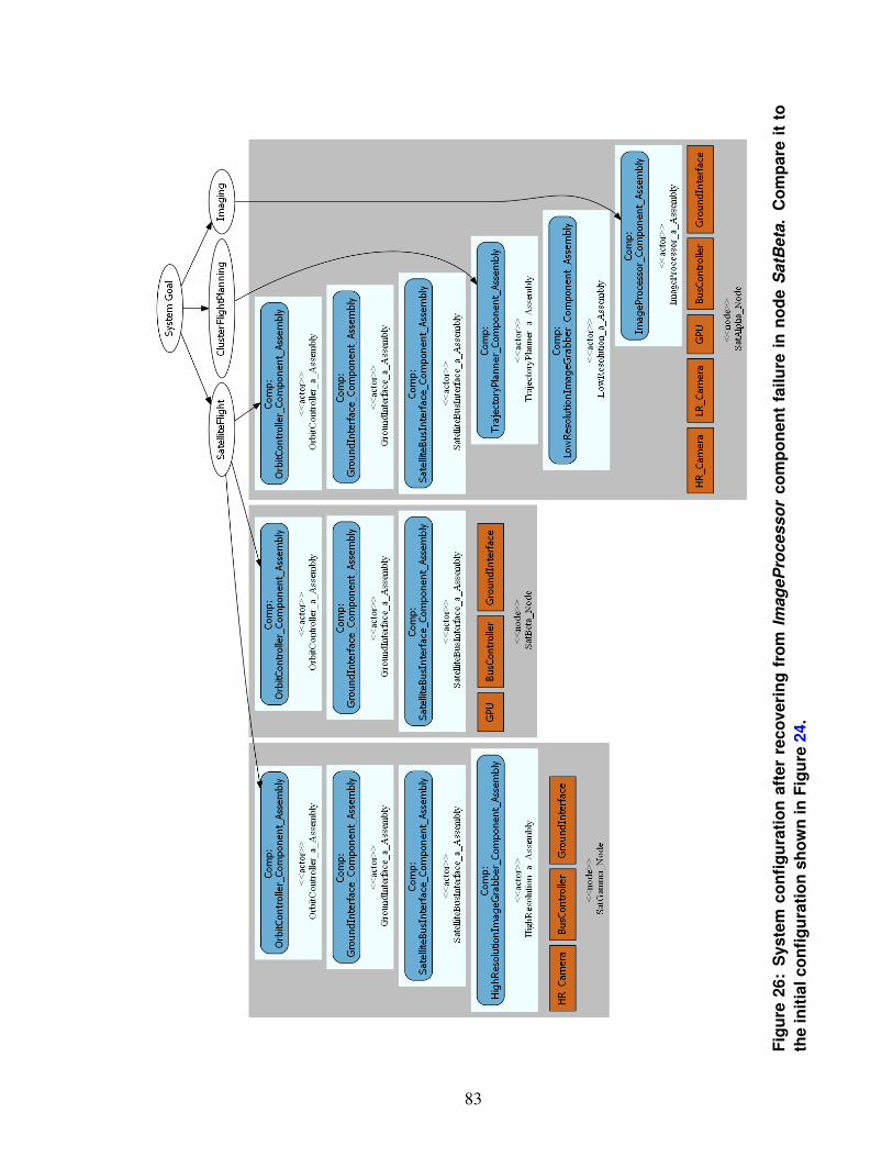
Figu
re26
:S
yste
mco
nfigu
ratio
naf
ter
reco
veri
ngfr
omIm
ageP
roce
ssor
com
pone
ntfa
ilure
inno
deS
atB
eta.
Com
pare
itto
the
initi
alco
nfigu
ratio
nsh
own
inFi
gure
24.
83

V.4.3 Runtime Self-Reconfiguration Mechanism Demonstration
In this section, we demonstrate the self-reconfiguration capability provided by our run-
time infrastructure. Figure 24 shows the system configuration after the initial deployment.
From this figure, it is clear that the system requires three different objectives – Satellite-
Flight, Imaging, and ClusterFlightPlanning – to satisfy its high-level goal. To test re-
silience, we first inject a component failure 1 by failing the ImageProcessor component in
node SatBeta. Once a Resilience Engine receives this failure report, it computes a new con-
figuration point and a list of reconfiguration commands to transition the system from its cur-
rent configuration point (faulty) to the new configuration point. In this particular scenario,
the Resilience Engine computes a solution that requires the ImageProcessor component
to be moved from node SatBeta to SatAlpha; this makes sense because the ImageProces-
sor component requires GPU device and the only other node with a GPU device is node
SatAlpha. The resulting configuration is presented in Figure 26.
V.4.4 Runtime Self-Reconfiguration Mechanism Evaluation
Figure 27 presents result of two experiments we performed to evaluate our self-reconfig-
uration mechanism. First, we compare the time taken to compute new configuration points
after failures in the system model presented in Figure 23. As shown in the Figure 27a,
we consider four failures; first two failures are component failures (ImageProcessor and
LowResolutionImageGrabber), third failure is a node failure (SatBeta), and fourth failure
is another component failure (TrajectoryPlanner). The time taken to compute a new con-
figuration point for all four failure cases is 0.34 seconds on average, with minimum 0.31
seconds and maximum 0.36 seconds. The range here is 50 milliseconds. This is because
all four failures are invoked in the same system, which means the size of the C2N matrix
will be the same.
Second, we compare the time taken to compute new configuration points for different
1Failure injection is as simple as changing the status of the device to mark it as failed.
84

(a) Configuration computation time forfailures in the simple system modelpresented in Figure 23.
(b) Average configuration computation time for four failures in dif-ferent system models. Both y-axis are in logarithmic scale.
Figure 27: Configuration computation time for failures in a simple model (left) andaverage configuration computation time for four failures in different system models(right). The different system models have increasing complexity; A has 3 nodes and13 components, B has 5 nodes and 19 components, C has 8 nodes and 28 compo-nents, D has 10 nodes and 34 components, E has 12 nodes and 40 components, Fhas 15 nodes and 49 components, and G has 18 nodes and 58 components.
system models. As shown in Figure 27b, we use seven different system models and for
each system model we compute the average configuration computation time with regards
to the same four failures that we used for our first evaluation experiment (Figure 27a).
Although all seven system models comprise similar nodes and components, the number of
nodes and components in each system model is different. System model A is the simplest
and resembles the basic system model shown in Figure 23; it comprises of 3 nodes and
13 components. System model B comprises 5 nodes and 19 components. System model
C comprises 8 nodes and 28 components. System model D comprises 10 nodes and 34
components. System model E comprises 12 nodes and 40 components. System model
F comprises 15 nodes and 49 components. System model G comprises 18 nodes and 58
85
components. So we can see that these system models have increasing complexity. As
we can clearly see in Figure 27b, systems with higher complexity have higher average
configuration computation time. This is because of the size of the C2N matrix over which
all constraints are encoded. Furthermore, the size of the C2N matrix also tells us about
the size of the resource matrices (R2C and R2N). Since, we are considering increasing
scale of the same system model, we can argue that the size of the R2C and R2N matrices
will also increase as the system complexity increases. So, the more complex a system, the
larger its configuration space (all three different matrices and corresponding constraints)
and therefore the increase in time taken by the underlying Z3 solver to find a solution.
Here, we would like to state that, although Figure 27b presents result based on single
iteration of the experiment, we were able to reproduce similar results for multiple iterations
of the same experiment.
From these results we can see that configuration computation time increases with in-
crease in system complexity. As such, we have to be careful when choosing what classes
of systems this solution is applied to. For example, it might not be feasible to use this
solution as it is to large-scale hard real-time systems. A variation of this approach, which
relies on solution pre-computation, can used to resolve this issue. Details of this solution
pre-computation approach is presented in Chapter VI.
V.5 Related Work
Significant amount of prior work has been done in order to achieve dynamically re-
configuring systems. [7, 12, 97] presents different policy-based approaches to achieving
dynamic reconfiguration. In [12], the authors present a policy-based framework that re-
quires mission specification, which describes how specific roles are assigned to different
nodes based on their credentials and capabilities, and how these roles should be re-assigned
in response to changes or failures. As such, this mission specification explicitly encodes
86

reconfiguration actions, i.e., role re-assignments, during design-time. [97] also follows sim-
ilar approach where declarative policies are used to specify adaptation. In [7], the authors
present a policy-based approach where each adaptation policy comprises rules, actions, and
the rate at which each rule should be evaluated. These approaches are different from ours,
as we do not explicitly encode reconfiguration actions at design-time; it is impossible to
cover all possible combinations of failure scenarios at design-time.
Alternative approaches to achieving dynamic reconfiguration include use of system
health management techniques [103]. Existing work that follows this approach includes [64],
which shows how system-wide mitigation can be performed based on reactive timed state
machines specified at design-time, using the results of a two-level fault-diagnoser [28].
A boolean encoding for reconfiguration using a search based strategy is presented in [61].
These approaches have similar limitations to aforementioned policy-based approaches since
the runtime reconfiguration mechanism depends on design-time specifications.
In [39, 107], the authors present a middleware that supports timely reconfiguration in
distributed real-time systems. Application Graph, which contains information about what
services are required and how they depend on each other, and Expanded Graph, which con-
tains information about different service implementations, are studied a priori at design-
time. As such, these solutions also have similar limitations to aforementioned solution
since runtime reconfiguration mechanism relies on artifacts computed at design-time.
In [11], the authors present a tool called Planit for deployment and reconfiguration of
component-based applications. Planit uses a temporal planner and is based on a sense-
plan-act model for fault detection, diagnosis, and reconfiguration to recover from runtime
application failures. As such, it is similar to our work presented in this chapter. In order to
facilitate the runtime planning, Planit allows modeling of both, implicit and explicit config-
urations at design-time. Although our reconfiguration mechanism is also based on implic-
itly encoded configuration (we call this configuration space), we capture this encoding in
a very generic manner. To be precise, we use a goal-based system description approach to
87

ensure loose coupling between requirements and actual software entities that fulfill those
requirement. However, in Planit, implicit encoding is defined in terms of low-level soft-
ware artifacts such as components and their connections. We believe that a solution for
extensible CPS needs to provide better flexibility to account for dynamism.
V.6 Concluding Remarks
This chapter presented a self-reconfiguration mechanism that can be used to facilitate
autonomous resilience, which is important for extensible CPS. The self-reconfiguration
mechanism, presented in this chapter, is based on dynamic constraints that represent a sys-
tem and a Satisfiability Modulo Theories (SMT) solver that makes use of those constraints
to compute valid system state in order to reconfigure a system.
The work presented in this chapter has couple of shortcomings. First, the self-reconfigu-
ration mechanism is non-deterministic since it uses a SMT solver, which essentially searches
a dynamic search space (i.e., collection of constraints that represents a system) at runtime.
On one hand, this technique is important as extensible CPS are dynamic and any recon-
figuration mechanism used should execute at runtime rather than at design-time when all
possible failures cannot be forecasted. While, on the other hand, this technique results
in long reconfiguration time when used for large-scale systems; this becomes problem-
atic for real-time systems as they have to be highly available, and therefore, cannot incur
long reconfiguration times. To address this issue, next chapter (Chapter VI) presents a
pre-computation-based variation of the mechanism presented in this chapter.
Second shortcoming of this work is that the design-time resilience analysis tool is not
part of the runtime self-reconfiguration mechanism. In an ideal solution, it is essential to
incorporate design-time analysis and validation tools to the runtime self-reconfiguration
mechanism because it is important to ensure that any reconfiguration solution computed at
runtime, by the self-reconfiguration mechanism, is valid. This is a complex problem and
will be part of the future work.
88

Note of Acknowledgement: The initial part of this work, which includes the underlying
idea of using various Satisfiability Modulo Theories (SMT) constraints and computing re-
silience metrics, was performed by Dr. Tihamer Levendovszky when he was a Research
Assistant Professor at Vanderbilt University. This work presents extension of his initial
contribution, as well as, a complete implementation and experiments for validation. His
contribution and guidance have been instrumental in completing this work.
V.7 Related Publications
1. Subhav Pradhan, Abhishek Dubey, Tihamer Levendovszky, Pranav Kumar, William
Emfinger, Daniel Balasubramanian, William Otte, and Gabor Karsai. Achieving Re-
silience in Distributed Software Systems via Self-Reconfiguration. Journal of Sys-
tems and Software (JSS 2016).
2. Subhav Pradhan, William Otte, Abhishek Dubey, Aniruddha Gokhale, and Gabor
Karsai. Towards a Resilient Deployment and Configuration Infrastructure for Frac-
tionated Spacecraft. Proc. of the 5th Workshop on Adaptive and Reconfigurable
Embedded Systems (APRES 2013), pages 29 - 32, Philadelphia, PA, USA.
3. Subhav Pradhan, Abhishek Dubey, Aniruddha Gokhale, and Martin Lehofer. WiP
Abstract: Platform for Designing and Managing Resilient and Extensible CPS. Proc.
of the 7th International Conference on Cyber-Physical Systems (ICCPS 2016), pages
1 - 1, Vienna, Austria.
89

CHAPTER VI
A HOLISTIC SOLUTION FOR MANAGING EXTENSIBLE CPS
VI.1 Motivation
This chapter presents a holistic solution, called CHARIOT (Cyber-pHysical Applica-
tion aRchItecture with Objective-based reconfiguraTion), for managing extensible CPS.
The motivation for the work presented in this chapter is the same as that of the previous
chapter (see Section V.1). This is because the work presented in this chapter extends the
work presented in the previous chapter by (1) using the concept of generic component types
during design-time and adding the capability to compute exact component instances from
available component types at runtime, (2) encoding redundancy patterns using Satisfiabil-
ity Modulo Theory (SMT) constraints, and (3) adding the capability to use a finite horizon
look-ahead strategy that pre-computes solution to significantly improve the performance of
the Configuration Point Computation (CPC) algorithm presented in previous chapter (see
Section V.3.3.2).
Furthermore, instead of using the same motivating scenario of a fractionated satellite
cluster, this chapter uses a different motivating scenario. Consider an indoor parking man-
agement system installed in a garage. This case study focuses on the vacancy detection
and notification functionality. This system is designed to make it easier for clients to use
parking facilities by tracking the availability of spaces in a parking lot and servicing client
parking requests by determining available parking spaces and assigning a specific parking
space to a client. We use this system as a running example throughout the rest of this
chapter to explain various aspects of CHARIOT. Figure 28 visually depicts this system;
it consists of a number of pairs of camera nodes (wireless camera) and processing nodes
90

(Intel Edison module mounted on Arduino board)1 placed on the ceiling to provide cover-
age for multiple parking spaces. Each pair of a camera and a processing node is connected
via a wired connection. In addition, the parking lot has an entry terminal node that drivers
interact with to as they enter the parking lot.
Figure 28: An Overview of the Parking Management System Case Study.
In addition to the hardware devices that comprises the system, Figure 28 also shows
a distributed application consisting of five different types of components deployed on the
hardware outlined above. An ImageCapture component runs on a camera node and pe-
riodically captures an image and sends it to an OccupancyDetector component that runs
on a processing node. An OccupancyDetector component detects vehicles in an image
and determines occupancy status of parking spaces captured in the image. For an Im-
ageCapture component to send images to an OccupancyDetector component, it must first
find the OccupancyDetector by using the LoadBalancer component, which also runs on
1https://www.arduino.cc/en/ArduinoCertified/IntelEdison
91

a processing node. The LoadBalancer component keeps track of the different Occupan-
cyDetector components available. After an OccupancyDetector component analyses an
image for occupancy status of different parking spaces, it sends the result to the Parking-
Manager component, which keeps track of occupancy status of the entire parking lot. The
ParkingManager component also runs on a processing node. The fifth and final component
comprising the smart parking application is the Client component, which runs on the entry
terminal and interacts with users to allow them to query, reserve, and use the parking lot.
VI.2 Problem Description
Similar to the previous chapter, the work presented in this chapter also focuses on
the problem of autonomous resilience for extensible CPS. The case study shown in Sec-
tion VI.1 motivates the need for orchestration middleware like CHARIOT to manage de-
ployment, execution, and update phases. For example, middleware capable of deploying
distributed applications is quite useful in a large multi-level parking garage. Likewise,
managing the life-cycle of previously deployed applications during the execution phase is
also important. Factors that could trigger execution phase management actions vary from
optimization to resilience. For example, it is essential to ensure that the ParkingManager
component is not a single point of failure, i.e., the smart parking system should not fail
if the ParkingManager component fails. We therefore require middleware that can de-
tect failures, determine if a failure affects the ParkingManager component, and if it does,
then autonomously reconfigure the system so that a ParkingManager component is always
available. Reconfiguration of an extensible CPS requires a certain amount of time, which
might not be acceptable for safety-critical, real-time systems. In such scenarios, the only
viable solution is to have redundant copies of applications.
Addressing the problems described above requires a solution that holistically addresses
92

both (1) the design-time challenges of capturing the system description, and (2) the run-
time challenges of implementing the dynamic reconfiguration strategies. In particular, the
following key factors must be considered by such a solution:
1. Failure avoidance, which is necessary since failures can cause downtime. Extensible
CPS consist of hardware components that degrade over time and hence eventually
fail. Likewise, software applications can also fail due to various defects. Since these
types of failures cannot be avoided altogether in an extensible CPS, one approach to
handling failure is to minimize its impact.
2. Failure management, which is needed to minimize downtime due to failures that
cannot be avoided, including failures caused by unanticipated changes. The desired
solution should ensure all application goals are satisfied for as long as possible, even
after failures.
3. Operations management, which is needed to minimize the challenges faced when
intentionally changing or evolving an existing extensible CPS, i.e., these are antic-
ipated changes. A solution for this should consider changes in hardware resources
and software applications.
VI.3 Solution Approach
This section presents detailed description of CHARIOT. First, an overview of the solu-
tion approach is presented, after which detailed description of the three different layers of
CHARIOT is presented.
VI.3.1 Overview of the Solution Approach
CHARIOT implements a three-layered architecture stack consisting of a design layer,
a data layer, and a management layer, as shown in Figure 29. The design layer is im-
plemented via a generic system description language that captures system specifications
in terms of different kinds of available hardware resources, software applications, and
93

the resource provided/required relationship between them. As described later in Sec-
tion VI.3.2, CHARIOT implements this layer using a domain-specific modeling language
(DSML) called CHARIOT-ML whose goal-based system description approach yields a
generic means of describing complex extensible CPS.
Figure 29: The Layered Architecture of CHARIOT.
In the middle of CHARIOT’s stack is a data layer implemented using a persistent data
storage and the corresponding well-defined schema to store system information, which
includes a design-time system description and a runtime representation of the system. This
layer canonicalizes the format in which information about extensible CPS is represented.
We present the details of this contribution in Section VI.3.3.
The bottom of CHARIOT’s stack is a management layer that comprises monitoring and
deployment infrastructures, as well as a novel management engine that facilitates applica-
tion (re)configuration as a mechanism to support autonomous resilience. As described later
in Section VI.3.4, this management engine uses system information stored in the persistent
storage to formulate Satisfiability Modulo Theories (SMT) constraints that encode system
94

properties and requirements, enabling the use of SMT solvers (such as Z3 [26]) to dynami-
cally compute optimal system (re)configuration at runtime. Here it is important to note that
the underlying technology and concept used for reconfiguration is similar to that presented
in the previous chapter (Chapter V). However, as previously mentioned in Section VI.1, the
work presented in this chapter is an extension of the previous chapter and has distinct novel
contributions.
CHARIOT handles failure avoidance via functionality redundancy and optimal distri-
bution of redundant functionalities. The general idea here is to be able to tolerate more
failures by strategically deploying redundant copies of components that provide critical
functionalities, such that more failures are avoided/tolerated without having to reconfigure
the system; further description of functionality redundancy is presented in Section VI.3.2.2.
Failure management is handled using the above-described sense-plan-act loop. The
Monitoring Infrastructure is responsible for detecting failures; this is the sensing phase.
After failure detection, it is the responsibility of the Management Engine to determine the
actions needed to reconfigure the system such that failures are mitigated; this is the plan-
ning phase and is based on Z3 [26], which is an open source Satisfiability Modulo Theories
(SMT) solver. Once reconfiguration actions are computed, the Deployment Infrastructure
is responsible for taking those actions to reconfigure the system; this is the acting phase.
Since failure detection and diagnosis have been extensively studied in existing literature,
the focus of this chapter is strictly on the second (planning) and third (acting) phases of
the self-reconfiguration loop; this is presented in Section VI.3.4. We use capabilities sup-
ported out-of-the-box by ZooKeeper [46] to implement a monitoring infrastructure based
on a group membership mechanism (see Setion VI.4.1.2).
Operations management is required to handle anticipated changes (i.e., planned update
or evolution). These changes include both hardware and software changes carried out at
runtime. Addition of new nodes and removal of existing nodes are example of hardware
changes. Similarly, addition of new applications, removal of existing applications, and
95

modification of existing applications are example of software changes. While failure man-
agement is triggered by detection of failures, operations management can be triggered for
various reason. A software related change is always instigated from changes made to the
appropriate design-time system model. So, for a software related change there is no detec-
tion mechanism; the trigger has to be human/manual invocation of the management engine.
However, in the case of a hardware related change, since hardware nodes are not modeled
explicitly as part of a design-time system model, some external entity is required to detect
these changes and invoke the management engine. This detection is also done by the group
membership mechanism presented in Section VI.4.1.2.
Figure 30: Reconfiguration Triggers associated with Failure Management and Op-erations Management.
To summarize detection and reconfiguration trigger mechanisms associated with fail-
ure management and operations management, we present Figure 30 as an overview. As
shown in the figure, reconfiguration for failure management and hardware update (opera-
tions management) is triggered by the monitoring infrastructure. Whereas, reconfiguration
for software update (operations management) is manually triggered once the system model
is updated.
96

VI.3.2 The CHARIOT Design Layer
This section describes the CHARIOT design layer, which addresses the requirement of
a design-time entity to capture system descriptions. CHARIOT’s design layer allows im-
plicit and flexible system description prior to runtime. In general, an extensible CPS can be
described in terms of required components or it could be described in terms of functionali-
ties provided by components. The former approach is inflexible since it tightly couples spe-
cific components with the system. CHARIOT therefore supports the latter approach, which
is more generic and flexible since it describes the system in terms of required functional-
ities, so that different components can be used to satisfy system requirements, depending
on their availability.
A key challenge we faced when creating CHARIOT was to devise a design-time en-
vironment whose system description mechanism could capture system information (e.g.,
properties, provisions, requirements, and constraints) without explicit management direc-
tives (e.g., if node A fails, move all components to node B). The purpose of this mechanism
is to enable CHARIOT to manage failures by efficiently searching for alternative solutions
at runtime. Another challenge we faced was how to devise abstractions that ensure both
correctness and flexibility so CHARIOT can easily support operations management.
To meet the challenges described above, CHARIOT’s design layer allows application
developers to model extensible CPS using a generic system description mechanism sup-
ported by CHARIOT-ML, which is our design-time modeling environment. We implement
this mechanism leveraging the goal-based system description approach described in previ-
ous chapter (see Section V.2.1). As shown in Figure 31, the key entities modeled as part
of a system’s description using CHARIOT-ML are: (1) hardware resource categories and
templates, (2) different types of components that provide various functionalities, and (3)
goal descriptions corresponding to different applications that must be hosted on available
resources. Since extensible CPS applications are generally mission-specific, their goals
97

should be satisfied during a specified amount of time. CHARIOT defines a goal as a col-
lection of objectives, where each objective is a collection of functionalities that can have
inter-dependencies.
Figure 31: CHARIOT-ML Modeling Concepts and their Dependencies.
CHARIOT’s design layer concretizes the functionality tree described in Section V.2.1.
It currently enforces a two-layer functionality hierarchy, where objectives are high-level
functionalities that satisfy goals and functionalities are leaf nodes associated with compo-
nent types. When these component types are instantiated, each component instance pro-
vides associated functionalities. To maximize composability and reusability, a component
type can only be associated with a single functionality, though multiple component types
can provide the same functionality.
To further elaborate CHARIOT’s design layer the remainder of this section presents
the system description of the smart parking system initially presented in Section VI.1.
Figure 32 shows the corresponding functionality tree, which is used below to describe the
different entities comprising the system’s description using snippets of models built using
CHARIOT-ML.
98

Figure 32: Parking System Description for the example shown in figure 28.
VI.3.2.1 Node Categories and Templates
Since physical nodes are part of an extensible CPS, CHARIOT-ML models them using
categories and templates. The nodes are not explicitly modeled since the group of nodes
comprising a system can change dynamically at runtime. The degree of dynamicity varies
from one system to another; for example, a smart parking system is far less dynamic when
compared to a fractionated satellite cluster. As such, in CHARIOT we only model node
categories and node templates. A node category can be defined as a logical concept used to
establish groups of nodes; every node that is part of a extensible CPS belongs to a certain
node category.
Since we do not explicitly model nodes at design-time, we use the concept of node
templates to represent the kinds of nodes that can belong to a category. Therefore, a node
category is a collection of node templates and a node template is a collection of generic
information (such as memory, CPU, devices, etc) that can be associated with any node
that is an instance of the node template. When a node joins a cluster at runtime the only
information it needs to provide (beyond node-specific network information) is which node
99

Figure 33: Snippet of Node Categories and Node Templates Declarations.
template it is an instance of. The concept of node categories becomes important when
assigning a per-node replication constraint (discussed in Section VI.3.2.2), which requires
that a functionality be deployed on each node of the given category.
Figure 33 presents the node categories and templates for the smart parking system. As
shown in this figure, there are three categories of nodes: CameraNode (line 3-10), Process-
ingNode (line 12-18), and TerminalNode (line 20-26). Each category contains one template
each. The CameraNode category contains a wifi_cam template that represents a Wi-Fi en-
abled wireless IP camera. The ProcessingNode category contains an Edison template that
represents an Edison board. The TerminalNode category contains an entry_terminal tem-
plate that represents a parking control station placed at an entrance of a parking space. This
scenario is consistent with the smart parking system described in Section VI.1.
VI.3.2.2 Goal Description
The goal description for the smart parking application is shown in Figure 34 . The
goal itself is declared as SmartParking (line 3). Following the goal declaration is a list
100

of the objectives required to satisfy the goal (line 5-6). Two objectives are defined in this
example: the ClientInteraction objective and the OccupancyChecking objective. The Cli-
entInteraction objective is related to the task of handling client parking requests, whereas
the OccupancyChecking objective is related to the task of determining the occupancy status
of different parking spaces.
Figure 34: Snippet of Smart Parking Goal Description Comprising Objectives andReplication Constraints.
In CHARIOT-ML, objectives are instantiations of compositions (see Section VI.3.2.3).
The ClientInteraction objective instantiates the client_interaction composition (line 5) and
the OccupancyChecking objective instantiates the occupancy_checking composition (line
6). A description of how we model these compositions in CHARIOT-ML is presented in
Section VI.3.2.3. After the objectives are modeled as part of a system, CHARIOT-ML al-
lows the association of those objectives’s functionalities with replication constraints. For
example, Figure 34 shows the association of the image_capture functionality with a per-
node replication constraint (line 9-10), which means this functionality should be present on
each node that is an instantiation of any node template belonging to CameraNode category.
Similarly, the parking_client functionality is also associated with a per-node replication
101
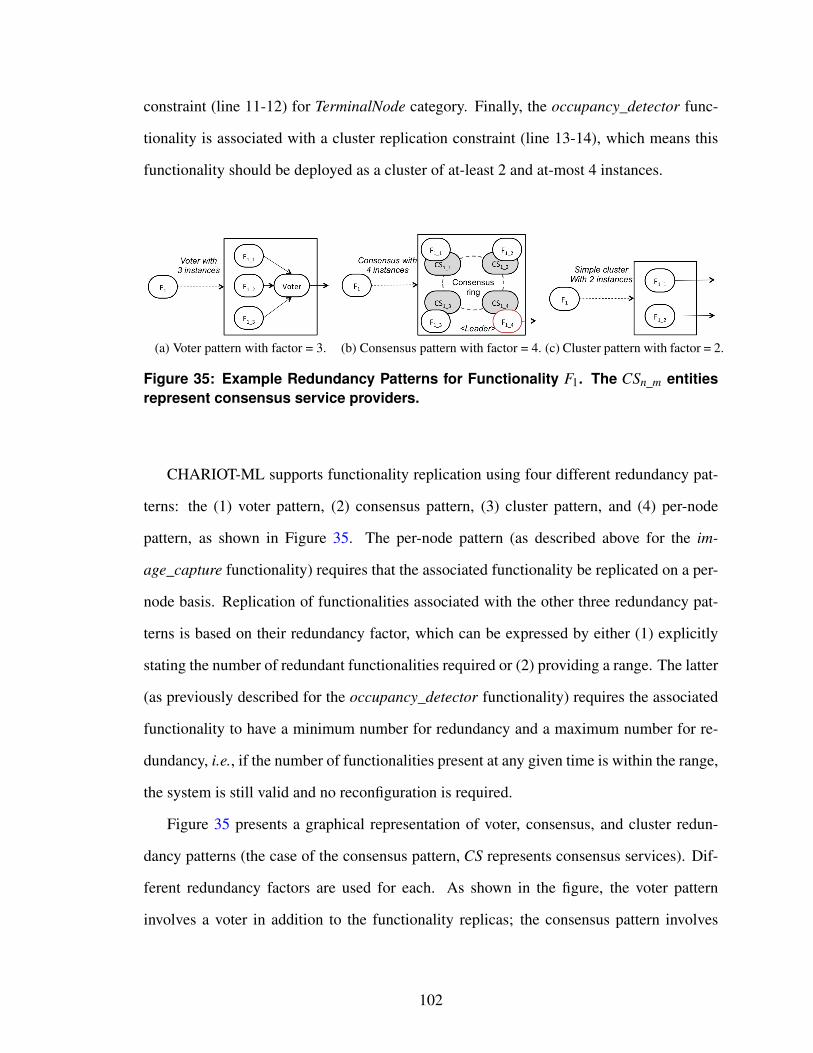
constraint (line 11-12) for TerminalNode category. Finally, the occupancy_detector func-
tionality is associated with a cluster replication constraint (line 13-14), which means this
functionality should be deployed as a cluster of at-least 2 and at-most 4 instances.
(a) Voter pattern with factor = 3. (b) Consensus pattern with factor = 4. (c) Cluster pattern with factor = 2.
Figure 35: Example Redundancy Patterns for Functionality F1. The CSn_m entitiesrepresent consensus service providers.
CHARIOT-ML supports functionality replication using four different redundancy pat-
terns: the (1) voter pattern, (2) consensus pattern, (3) cluster pattern, and (4) per-node
pattern, as shown in Figure 35. The per-node pattern (as described above for the im-
age_capture functionality) requires that the associated functionality be replicated on a per-
node basis. Replication of functionalities associated with the other three redundancy pat-
terns is based on their redundancy factor, which can be expressed by either (1) explicitly
stating the number of redundant functionalities required or (2) providing a range. The latter
(as previously described for the occupancy_detector functionality) requires the associated
functionality to have a minimum number for redundancy and a maximum number for re-
dundancy, i.e., if the number of functionalities present at any given time is within the range,
the system is still valid and no reconfiguration is required.
Figure 35 presents a graphical representation of voter, consensus, and cluster redun-
dancy patterns (the case of the consensus pattern, CS represents consensus services). Dif-
ferent redundancy factors are used for each. As shown in the figure, the voter pattern
involves a voter in addition to the functionality replicas; the consensus pattern involves
102
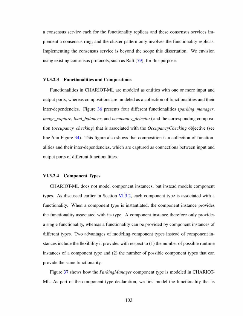
a consensus service each for the functionality replicas and these consensus services im-
plement a consensus ring; and the cluster pattern only involves the functionality replicas.
Implementing the consensus service is beyond the scope this dissertation. We envision
using existing consensus protocols, such as Raft [79], for this purpose.
VI.3.2.3 Functionalities and Compositions
Functionalities in CHARIOT-ML are modeled as entities with one or more input and
output ports, whereas compositions are modeled as a collection of functionalities and their
inter-dependencies. Figure 36 presents four different functionalities (parking_manager,
image_capture, load_balancer, and occupancy_detector) and the corresponding composi-
tion (occupancy_checking) that is associated with the OccupancyChecking objective (see
line 6 in Figure 34). This figure also shows that composition is a collection of function-
alities and their inter-dependencies, which are captured as connections between input and
output ports of different functionalities.
VI.3.2.4 Component Types
CHARIOT-ML does not model component instances, but instead models component
types. As discussed earlier in Section VI.3.2, each component type is associated with a
functionality. When a component type is instantiated, the component instance provides
the functionality associated with its type. A component instance therefore only provides
a single functionality, whereas a functionality can be provided by component instances of
different types. Two advantages of modeling component types instead of component in-
stances include the flexibility it provides with respect to (1) the number of possible runtime
instances of a component type and (2) the number of possible component types that can
provide the same functionality.
Figure 37 shows how the ParkingManager component type is modeled in CHARIOT-
ML. As part of the component type declaration, we first model the functionality that is
103

Figure 36: Snippet of Functionalities and Corresponding Composition Declaration.
Figure 37: Snippet of Component Type Declaration.
104

provided by the component (line 4). After the functionality of a component type is modeled,
we model various resource requirements (Figure 37 only shows memory requirements in
line 6) and the launch script (line 8), which can be used to instantiate an instance of the
component by spawning an application process.
CHARIOT supports two different types of component types: hardware components
and software components. The component type presented in Figure 37 is an example of a
software component. Hardware components are modeled in a similar fashion, though we
just model the functionality provided by a hardware component and nothing else since a
hardware component is a specific type of component whose lifecycle is tightly coupled to
the node with which it is associated. A hardware component is therefore never actively
managed (reconfigured) by the CHARIOT orchestration middleware. The only thing that
affects the state of a hardware node is the state of its hosting node, i.e., if the node is on and
functioning well, the component is active and if it is not, then the component is inactive.
In context of the smart parking system case study presented in this chapter, the Image-
Capture component is a hardware component that is associated with camera nodes. As
a result, an instance of the ImageCapture component runs on each active camera node.
We model this requirement using the per-node redundancy pattern (see line 32-33 in Fig-
ure 34). Likewise, the failure of a camera node implies failure of the hosted ImageCapture
component instance, so this failure cannot be mitigated.
VI.3.3 The CHARIOT Data Layer
This section presents the CHARIOT data layer, which defines a schema that forms the
basis for persistently storing system information, such as design-time system description
and runtime system information. This layer codifies the format in which system infor-
mation should be represented. A key advantage of this codification is its decoupling of
CHARIOT’s design layer (top layer) from its management layer (bottom layer), which
yields a flexible architecture that can accommodate varying implementations of the design
105

layer, as long as those implementations adhere to the data layer schema described in this
section.
(a) Schema to Store Design-time System Descriptions.
(b) Schema to Store Runtime System Representations.
Figure 38: UML Class Diagrams for Schemas Used to Store System Information.
Figure 38 presents UML class diagrams as schemas used to store design-time system
description and runtime system information. These schemas are designed for document-
oriented databases. An instance of a class that is not a child in a composition relationship
106
therefore represents a root document. Below we describe CHARIOT’s design-time and
runtime schemas in detail.
VI.3.3.1 Design-time System Description Schema
The schema for design-time system description comprises entities to store node cate-
gories, component types, and goal descriptions, as shown in Figure 38a. As discussed in
Section VI.3.2.1, a node category is a concept used to establish logical groups of nodes that
form part of an extensible CPS. It contains a collection of node templates, which provide
a generic specification of a type of node. The NodeCategory class therefore consists of
a unique name and a list of node templates. Likewise, the NodeTemplate class consists
of a unique name and a set of specification attributes, such as available operating system,
middleware, memory, storage, software artifacts, and devices.
In addition to node categories, a design-time system description schema also captures
component types available for extensible CPS applications. Neither node categories nor
component types are application-specific since multiple applications can be simultaneously
hosted on nodes of an extensible CPS and a component type can be used by multiple ap-
plications.The ComponentType class consists of a unique name and a set of other attributes
such as (1) name of the functionality provided, (2) required operating system, middleware,
memory, storage, software artifacts, and required devices, and (3) scripts that can be used
to start and stop an instance of the component type, as shown in Figure 38a.
A design-time system description schema also consists of goal descriptions. As dis-
cussed in Section VI.3.2, a goal description is application-specific and it describes the goal
of an application in terms of objectives and functionalities required to satisfy the goal. The
GoalDescription class consists of a unique name and a set of objectives and constraints, as
shown in Figure 38a. Moreover, objectives are represented by the Objective class,w hich
consists of a unique name and a set of functionalities.
107

In addition to objectives and functionalities, a goal description can also contain repli-
cation constraints. The ReplicationConstraint class represents replication constraints, as
shown in Figure 38a. As described in Section VI.3.2.2, a replication constraint has a kind,
which can either be a voter, consensus, cluster, or per-node. A replication constraint should
always be associated with a functionality. The maxInstances, minInstance, and numIn-
stances attributes are related to the degree of replication. The latter attribute is used if a
specific number of replica is required, whereas the former two attributes are used to de-
scribe a range-based replication. The nodeCategories attribute is used for per-node repli-
cation constraints. The serviceComponentType attribute is related to specific component
types that provide special replication services, such as a component type that provides a
voter service or a consensus service.
VI.3.3.2 Runtime System Information Schema
The schema for runtime system information comprises entities to store functionality
instances, nodes, deployment actions, reconfiguration events, and look-ahead information,
as shown in Figure 38b. The FunctionalityInstance class consists of a unique name, name
of the associated functionality and objective, boolean flags to indicate whether a func-
tionality instance corresponds to the voter of a voter replication group (isVoter attribute)
or a consensus service provider of a consensus replication group (isConsensusProvider).
The FunctionalityInstance class also consists of a ComponentType attribute to store exact
component type of a functionality instance; this attribute is only relevant for voter and con-
sensus service providing functionality instances as they are not associated with a separate
functionality that is part of a goal description. Furthermore, the FunctionalityInstance class
also consists of an alwaysDeployOnNode attribute, which ties a functionality instance to a
specific node and is only relevant for functionality instances related to per-node replication
groups. Finally, a mustDeploy boolean attribute of the FunctionalityInstance class indicates
whether a functionality instance should always be deployed.
108

The Node class consists of a unique name, associated node template, node status, and
a list of hosted processes. For the latter, the Process class is used and it consists of a
unique name, process ID, status, and a list of hosted component instances. Similarly, the
ComponentInstance class represents component instances and it consists of a unique name,
name of the component type it implements, status, name of the corresponding functionality
instance as a component instance is always associated with a functionality instance (see
Section VI.3.4.2), node name (alwaysDeployOnNode) if a component instance needs to be
always deployed on that node as part of a per-node replication constraint, and a mustDeploy
boolean attribute to determine if a component instance must always be deployed.
The DeploymentAction class represents runtime deployment actions that are computed
by the CHARIOT management engine to (re)configure a system. The DeploymentAction
class consists of an action, a completed boolean flag to indicate if an action has been taken
or not, process affected by the action, node on which the action should be performed, and
scripts to perform the action. CHARIOT supports two kinds of actions: start actions and
stop actions. The LookAhead class represents pre-computed solutions related to CHAR-
IOT’s finite-horizon look-ahead strategy described in Section VI.3.4.3. It consists of at-
tributes that represents a failed entity, and a set of recovery actions (deployment actions)
that must be performed to recover from the failure.
Finally, the ReconfigurationEvent class represents runtime reconfiguration events. It is
used to keep track of different failure and update events that triggers system reconfigura-
tion. It consists of detectionTime, solutionFoundTime, and reconfiguredTime to keep track
of when a failure or update was detection, when a solution was computed, and when the
computed solution was deployed. It also consists of a completed boolean attribute to in-
dicate whether a reconfiguration event is complete or not and an actionCount attribute to
keep track of number of actions required to complete a reconfiguration event.
109

VI.3.4 The CHARIOT Management Layer
The CHARIOT management layer comprises a monitoring infrastructure, deployment
infrastructure, and a management engine, as shown in Figure 29. The monitoring, deploy-
ment, and configuration of distributed applications are well studied, so CHARIOT imple-
ments these capabilities using existing technologies, as described in Section VI.4.1. This
section therefore focuses on CHARIOT’s management engine, which is a novel contribu-
tion that facilitates self-reconfiguration of extensible CPS managed via CHARIOT.
VI.3.4.1 Configuration Space and Points
The general idea behind CHARIOT’s self-reconfiguration approach is similar to that
presented in the previous chapter (see Section V.2.3.2). As such the self-reconfiguration
approach relies on the concepts of configuration space and configuration points. If a sys-
tem’s state is represented by a configuration point in a configuration space, then reconfig-
uration of that system entails moving from one configuration point to another in the same
configuration space. The remainder of this section describes these concepts and presents
CHARIOT’s core reconfiguration mechanism and configurable look-ahead strategy.
For the work presented in this chapter we consider a configuration space to include (1)
goal descriptions of different application, (2) replication constraints corresponding to re-
dundancy patterns associated with different applications, (3) component types that can be
used to instantiate different component instances and therefore applications, and (4) avail-
able resources, which includes different nodes and their corresponding resources, such as
memory, storage, and computing elements. At any given time a configuration space of
an extensible CPS can represent multiple applications associated with the system. A con-
figuration space can therefore contain multiple configuration points, which represent valid
configurations of all applications that are part of the system represented by the configura-
tion space.
110

A configuration point is a valid configuration of a system which represents component-
instance-to-node mappings (i.e., a deployment) for all component instances needed to re-
alize different functionalities essential for the objectives required to satisfy goals of one or
more applications. The initial configuration point represents the initial (baseline) deploy-
ment, whereas, current configuration point represents the current deployment.
VI.3.4.2 Computing the Configuration Points
Given the description of configuration space and points, a valid reconfiguration mecha-
nism should be based on transitions between configuration points. The Configuration Point
Computation (CPC) algorithm serves this purpose and thus defines the core of CHARIOT’s
self-reconfiguration mechanism. Although a version of the CPC algorithm is presented in
the previous chapter (see Section V.3.3.2), the version of the CPC algorithm presented in
this section (1) extends the prior version by accounting for the concept of abstract compo-
nent types and generating concrete component instances out of them, and (2) describes the
SMT constraint encodings in much more detail. As such, the CPC algorithm presented in
this section can be decomposed into three phases: the (1) instance computation phase, (2)
constraint encoding phase, and (3) solution computation phase, as described below.
Phase 1, Instance Computation Phase:
The first phase of a CPC computes required instances of different functionalities and sub-
sequently components, based on the system description provided at design-time. Each
functionality can have multiple instances if it is associated with a replication constraint.
Each functionality instance should have a corresponding component instance that provides
the functionality associated with the functionality instance. Depending upon the number of
component types that provide a given functionality, a functionality instance can have multi-
ple component instances. Only one of the component instances will be deployed at runtime,
however, so there is always be a one-to-one mapping between a functionality instance and
a deployed component instance.
111

The CPC algorithm first computes different functionality instances using Algorithm 5,
which is invoked for each objective. Every functionality is initially checked for replica-
tion constraints (line 3). If a functionality does not have a replication constraint, a single
functionality instance is created (line 32). For every functionality that has one or more
replication constraints associated with it, we handle each constraint depending on the type
of the constraint. A per-node replication constraint is handled by generating a functional-
ity instance and an assign constraint each for applicable nodes (line 6-11). An application
node is a node that is alive and belongs to the node category associated with the per-node
replication constraint.
Algorithm 5 Functionality Instances Computation.Input: objective (ob j), nodes (nodes_list), computed functionalities(computed_ f unctionalities)Output: functionality instances for ob j (ret_list)1: for f unc in ob j. f unctionalities do2: if f unc not in computed_ f unctionalities then . Make sure a functionality is processed only once.3: if f unc has associated replication constraints then4: constraints = all replication constraints associated with f unc5: for c in constraints do6: if c.kind == PER_NODE then . Handle per node replication.7: for node_category in c.nodeCategories do8: nodes = nodes in nodes_list that are alive and belong to category node_category9: for n in nodes do10: create functionality instance and add it to ret_list11: add assign (functionality instance, n) constraint12: else13: replica_num = 0 . Initial number of replicas, which will be set to max value if range given.14: range_based = False . Flag to indicate if a replication constraints is range based.15: if c.numInstances ! = 0 then16: replica_num = c.numInstances17: else18: range_based = True19: replica_num = c.maxInstances20: for i = 0 to replica_num do . Create replica functionality instances.21: create replica functionality instance and add it to ret_list22: if c.kind ==CONSENSUS then . Handle consensus replication.23: create consensus service functionality instance and add it to ret_list24: add implies (replica functionality instance, consensus service functionality instance) constraint25: add collocate (replica functionality instance, consensus service functionality instance) constraint26: if c.kind ==VOT ER then . Handle voter replication.27: create voter functionality instance and add it to ret_list28: if range_based == True then . If replication range is given, add atleast constraints.29: add atleast (c.rangeMinValue, replica functionality instances) constraint30: add distribute (replica functionality instances) constraint31: else32: create functionality instance and add it to ret_list33: add f unc to computed_ f unctionalities
Unlike a per-node replication constraint, the voter, consensus, and cluster replication
112
constraints depend on exact replication value or replication range to determine the number
of replicas (line 13-19). In the case of a range-based replication, CHARIOT tries to maxi-
mize the number of replicas by using maximum of the range, which ensures that maximum
number of failures are tolerated without having to reconfigure the system. After the num-
ber of replicas is determined, CHARIOT computes the replica functionality instances (line
21), as well as special functionality instances that support different kinds of replication
constraint. For example, for each replica functionality instance in a consensus replication
constraint, CHARIOT generates a consensus service functionality instance (line 23) (a con-
sensus service functionality is provided by a component that implements consensus logic
using existing algorithms, such as Paxos [53], Raft [79]). For a voter replication constraint,
in contrast, CHARIOT generates a single voter functionality instance for the entire replica-
tion group (line 27). In the case of a cluster replication constraint, no special functionality
instance is generated as a cluster replication comprises independent functionality instances
that do not require any synchronization (see Section VI.3.2.2).
To ensure proper management of instances related to functionalities with voter, consen-
sus, or cluster replication constraints, CHARIOT uses four different constraints: (1) im-
plies, (2) collocate, (3) atleast, and (4) distribute. The implies constraint ensures all replica
functionality instances associated with a consensus pattern require their corresponding con-
sensus service functionality instances (line 24). Similarly, the collocate constraint ensures
each replica functionality instance and its corresponding consensus service functionality in-
stance are always collocated on the same node (line 25). The atleast constraint ensures the
minimum number of replicas are always present in scenarios where a replication range is
provided (line 28-29). Finally, the distribute constraint ensures that the replica functionali-
ties are distributed across different nodes (line 30). CHARIOT’s ability to support multiple
instances of functionalities and distribute them across nodes enables failure avoidance.
After functionality instances are created, CHARIOT next creates the component in-
stances corresponding to each functionality instance. In general, it identifies a component
113

type that provides the functionality associated with each functionality instance and instanti-
ates that component type. As explained in Section VI.3.2.4, component types are modeled
as part of the system description. Different component types can provide the same func-
tionality, in which case multiple component types are instantiated, but a constraint is added
to ensure only one of those instances is deployed and running at any given time. In ad-
dition, all constraints previously created in terms of functionality instances are ultimately
applied in terms of corresponding component instances. Detailed description of how these
constraints are encoded is provided below.
Phase 2, Constraint Encoding Phase:
The second phase of the CPC algorithm is responsible for constraint encoding and opti-
mization. The goal is to represent the configuration space and current configuration point
using a set of constraints, which allows CHARIOT to use solvers to compute a new con-
figuration point by solving these constraints. The CHARIOT management engine uses
Satisfiability Modulo Theories (SMT) [15] for constraint encoding and optimization; its
underlying solver is Z3 [26]. To present a generic solution, we first identify a set of con-
straints and optimization that are required:
1. Since reconfiguration involves transitioning from one configuration point to another,
constraints that represent a configuration point are of utmost importance.
2. Constraints to ensure component instances that must be deployed are always de-
ployed.
3. Constraints to ensure component instances that communicate with each other are
either deployed on the same node or on nodes that have network links between them.
4. Constraints to ensure resources provided-required relationships are valid.
5. Constraints encoded in the first phase of the CPC algorithm for proper management
of component instances associated with replication constraints.
6. Constraints to represent failures, such as node failure or device failures.
The remainder of this section describes how CHARIOT implements the constraints
114

listed above as SMT constraints. These constraints are generic constraints (also presented
briefly in previous chapter, see Table 6) that apply to extensible CPS in different domains,
though more constraints can be added for special needs of specific domains. For example,
given the availability of period and deadline of all component instances, an extensible CPS
with stringent real-time deadlines might require a specific resource constraint that ensures
periodic scheduling of applications, e.g., using Rate Monotonic Scheduling or another real-
time scheduling algorithm.
As mentioned in Section VI.3.4.1, a configuration point represents a valid deployed
of all component instances. A configuration point in CHARIOT is therefore presented
using a component-instance-to-node (C2N) matrix, as shown in the previous chapter (see
Section V.2.3.2).
Now we need a constraint to ensure component instances that should be deployed are
always deployed. At this point it is important to recall range-based replication described
in Section VI.3.2.2, which results in a set of instances where a certain number (at least the
minimum) should always be deployed, but the remaining (difference between maximum
and minimum) are not always required, even though all of them are deployed initially. At
any given time, therefore, a configuration point can comprise of some component instances
that must be deployed and others that are not always required be deployed. In CHARIOT
we encode the must deploy constraint as follows:
Definition 10 (Must deploy assignment). The “must deploy assignment” constraint is used
to ensure all component instances that should be deployed are in fact deployed. This con-
straint therefore uses the C2N matrix (Equation V.1) and a set of component instances that
must be deployed, as shown in Equation VI.1.
Let M be a set of all component instances that must be deployed.
∀m ∈M :β
∑n=0
c2nmn == 1 (VI.1)
115

The third set of constraints we need ensure that component instances with inter-dependencies
(i.e., that communicate with each other) are either deployed on the same node or on nodes
that have network links between them. CHARIOT encodes this constraint as follows:
Definition 11 (Dependency Constraint). This constraint ensures that interacting compo-
nent instances are always deployed on resources with appropriate network links to support
communication. This constraint is encoded in terms of two matrices: a node-to-node (N2N)
matrix and a component-instance-to-component-instance (C2C) matrix. The N2N matrix
represents network links between nodes and therefore comprises rows and columns that
represent different nodes (Equation VI.2). Each element of the N2N matrix is either 0 or
1, where 0 means there exists no link and 1 means there a link exists between the corre-
sponding nodes. The C2C matrix is the same except it comprises rows and columns that
both represent component instances (Equation VI.3). The constraint itself is presented in
Equation VI.4.
N2N =
n2n00 n2n01 n2n02 . . . n2n0β
n2n10 n2n11 n2n12 . . . n2n1β
. . . . . . . . . . . . . . . .
n2nβ0 n2nβ1 n2nβ2 . . . n2nββ
=
n2nn1n2 : (n1,n2) ∈ {0 . . .β},β ∈ Z+ (VI.2)
C2C =
c2c00 c2c01 c2c02 . . . c2c0α
c2c10 c2c11 c2c12 . . . c2c1α
. . . . . . . . . . . . . . . .
c2cα0 n2nα1 n2nα2 . . . n2nαα
=
c2cc1c2 : (c1,c2) ∈ {0 . . .α},α ∈ Z+ (VI.3)
116

Let cs and cd be two component instances that are dependent on each other.
∀n1,∀n2 : ((c2ncsn1× c2ncdn2)∧ (n1 6= n2)) =⇒
(n2nn1n2 == c2ccscd)
(VI.4)
The fourth set of constraints CHARIOT needs ensure the validity of resources provided-
required relationships, such that essential component instances of one or more applications
can be provisioned. CHARIOT encodes these constraints in terms of resources provided
by nodes and required by component instances. Moreover, resources are classified into two
categories: (1) cumulative resources and (2) comparative resources. Cumulative resources
have a numerical value that increases or decreases depending on whether a resource is
used or freed. Examples of cumulative resources include primary memory and secondary
storage. Comparative resources have a boolean value, i.e., they are either available or
not available and their value does not change depending on whether a resource is used or
freed. Examples of comparative resources include devices and software artifacts. These
two constraints can be encoded as follows:
Definition 12 (Cumulative resource constraint). The “cumulative resource” constraint is
encoded using a provided resource-to-node (CuR2N) matrix and a required resource-to-
component-instance (CuR2C) matrix. The CuR2N matrix comprises rows that represent
different cumulative resources and columns that represent nodes; the size of this matrix is
γ × β , where γ is the number of cumulative resources and β is the number of available
nodes (Equation VI.5). The CuR2C matrix comprises rows that represent different cumu-
lative resources and columns that represent component instances; the size of this matrix is
γ ×α , where γ is the number of cumulative resources and α is number of component in-
stances (Equation VI.6). Each element of these matrices are integers. The constraint itself
(Equation VI.7) ensures that for each available cumulative resource and node, the sum of
117

the amount of the resource required by the component instances deployed on the node is
less than or equal to the amount of the resource available on the node.
CuR2N =
r2n00 r2n01 r2n02 . . . r2n0β
r2n10 r2n11 r2n12 . . . r2n1β
. . . . . . . . . . . . . . .
r2nγ0 r2nγ1 r2nγ2 . . . r2nγβ
=
r2nrn : r ∈ {0 . . .γ},n ∈ {0 . . .β},(γ,β ) ∈ Z+ (VI.5)
CuR2C =
r2c00 r2c01 r2c02 . . . r2c0α
r2c10 r2c11 r2c12 . . . r2c1α
. . . . . . . . . . . . . .
r2cγ0 r2cγ1 r2cγ2 . . . r2cγα
=
r2crc : r ∈ {0 . . .γ},c ∈ {0 . . .α},(γ,α) ∈ Z+ (VI.6)
∀r,∀n :
(α
∑c=0
c2ncn× r2crc
)≤ r2nrn (VI.7)
Definition 13 (Comparative resource constraint). The “comparative resource” constraint
is encoded using a provided resource-to-node (CoR2N) matrix and a required resource-to-
component-instance (CoR2C) matrix. The CoR2N matrix comprises rows that represent
different comparative resources and columns that represents nodes; the size of this matrix
is φ ×β , where φ is the number of comparative resources and β is the number of available
nodes (Equation VI.8). Similarly, the CoR2C matrix comprises rows that represent different
comparative resources and columns that represent component instances; the size of this
matrix is φ ×α , where φ is the number of comparative resources and α is number of
component instances (Equation VI.9). Each element of these matrices are either 0 or 1; 0
118

means the corresponding resource is not provided by the corresponding node (for CoR2N
matrix) or not required by the corresponding component instance (for CoR2C matrix),
whereas, 1 means the opposite. The constraint itself (Equation VI.10) ensures that for each
available comparative resource, node, and component instance, if the component instance
is deployed on the node and requires the resource, then the resource must also be provided
by the node.
CoR2N =
r2n00 r2n01 r2n02 . . . r2n0β
r2n10 r2n11 r2n12 . . . r2n1β
. . . . . . . . . . . . . . .
r2nφ0 r2nφ1 r2nφ2 . . . r2nφβ
=
r2nrn : r ∈ {0 . . .φ},n ∈ {0 . . .β},(φ ,β ) ∈ Z+ (VI.8)
CoR2C =
r2c00 r2c01 r2c02 . . . r2c0α
r2c10 r2c11 r2c12 . . . r2c1α
. . . . . . . . . . . . . . .
r2cφ0 r2cφ1 r2cφ2 . . . r2cφα
=
r2crc : r ∈ {0 . . .φ},c ∈ {0 . . .α},(φ ,α) ∈ Z+ (VI.9)
∀r,∀n,∀c : Assigned(c,n) =⇒ (r2nrn == r2crc) (VI.10)
Assigned (c, n) function returns true if component c is deployed on node n, i.e., it returns
true if c2ncn == 1.
The fifth set of constraints are needed for management of component instances asso-
ciated with replication constraints. As mentioned previously, assign, implies, collocate,
119
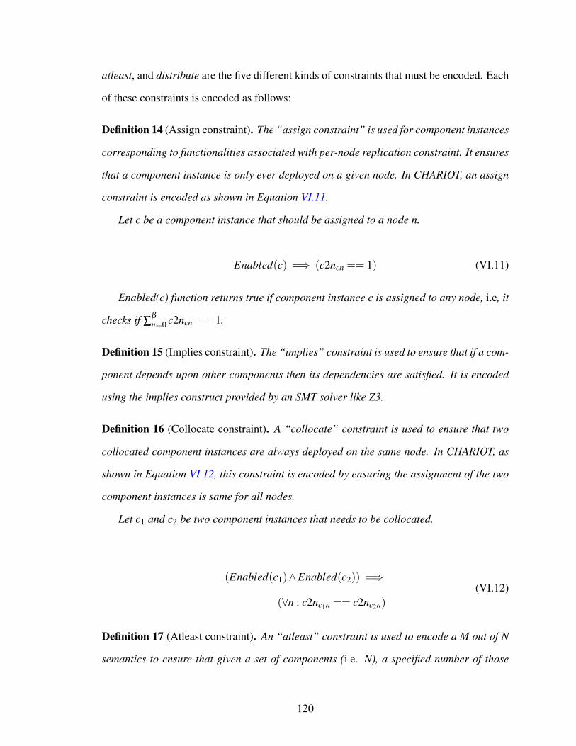
atleast, and distribute are the five different kinds of constraints that must be encoded. Each
of these constraints is encoded as follows:
Definition 14 (Assign constraint). The “assign constraint” is used for component instances
corresponding to functionalities associated with per-node replication constraint. It ensures
that a component instance is only ever deployed on a given node. In CHARIOT, an assign
constraint is encoded as shown in Equation VI.11.
Let c be a component instance that should be assigned to a node n.
Enabled(c) =⇒ (c2ncn == 1) (VI.11)
Enabled(c) function returns true if component instance c is assigned to any node, i.e, it
checks if ∑β
n=0 c2ncn == 1.
Definition 15 (Implies constraint). The “implies” constraint is used to ensure that if a com-
ponent depends upon other components then its dependencies are satisfied. It is encoded
using the implies construct provided by an SMT solver like Z3.
Definition 16 (Collocate constraint). A “collocate” constraint is used to ensure that two
collocated component instances are always deployed on the same node. In CHARIOT, as
shown in Equation VI.12, this constraint is encoded by ensuring the assignment of the two
component instances is same for all nodes.
Let c1 and c2 be two component instances that needs to be collocated.
(Enabled(c1)∧Enabled(c2)) =⇒
(∀n : c2nc1n == c2nc2n)
(VI.12)
Definition 17 (Atleast constraint). An “atleast” constraint is used to encode a M out of N
semantics to ensure that given a set of components (i.e. N), a specified number of those
120

components (i.e. M) is always deployed. CHARIOT only uses this constraint for range-
based replication constraints and its implementation is two fold. First, during the initial
deployment CHARIOT tries to maximize M and deploy as many component instances as
possible. Current implementation of CHARIOT uses the maximum value associated with a
range and initially deploys N component instances, as shown in Equation VI.13. This of
course assumes availability of enough resources. A better solution to this would be to use
the maximize optimization, as shown in EquationVI.14. However, in Z3 solver, which is the
SMT solver used by CHARIOT, this optimization is experimental and does not scale well.
Second, for subsequent non-initial deployment CHARIOT relies on the fact that maximum
possible deployment was achieved during initial deployment, so it ensures the minimum
number required is always met, as shown in Equation VI.15.
Let S= {c1,c2 . . .cα ′} be a set of replica component instances associated with an atleast
constraint; N is the size of this set. Also, let min_value be the minimum number of compo-
nent instances required; this is synonymous to M.
∑c∈S
β
∑n=0
c2ncn == max_value (VI.13)
maximize(∑c∈S
β
∑n=0
c2ncn) (VI.14)
∑c∈S
β
∑n=0
c2ncn >= min_value (VI.15)
Definition 18 (Distribute constraint). A “distribute” constraint is used to ensure that a set
of components are deployed on different nodes. In CHARIOT this constraint is encoded by
ensuring at most only one component instance out of the set is deployed on a single node,
as shown in Equation VI.16.
Let S = {c1,c2 . . .cα ′} be a set of components that needs to be distributed.
121

∀n : ∑c∈S
c2ncn ≤ 1 (VI.16)
The final step (step 8) of the second phase of the CPC algorithm encodes and adds
failure constraints. Depending on the kind of failure, there can be different types of failure
constraints. We describe how CHARIOT encodes node failures and component failures
below.
Finally, the sixth set of constraints handles failure representation. Constraints related to
different failures are encoded in CHARIOT as shown below:
Definition 19 (Node failure constraint). A “node failure” constraint is used to ensure that
no components are deployed on a failed node. CHARIOT encodes this constraint as shown
in Equation VI.17.
Let n f be a failed node.
α
∑c=0
c2ncn f == 0 (VI.17)
Definition 20 (Component failure constraint). A component can fail for various reasons,
so there can be different ways to resolve a component failure. One approach is to ensure
that a component is redeployed on any node other than the node in which it failed (Equa-
tion VI.18). If a component keeps failing in multiple different nodes, however, then CHAR-
IOT may need to consider another constraint that ensures the component is not redeployed
on any node (Equation VI.19).
Let us assume component c1 failed on node n1.
c2nc1n1==0 (VI.18)
β
∑n=0
c2nc1n == 0 (VI.19)
122
Phase 3, Solution Computation Phase:
The third and final phase of the CPC algorithm involves computing a “least distance” con-
figuration point, i.e., a configuration point that is the least distance away from current con-
figuration point. To achieve this, we leverage the least distance constraint (see Definition 9)
and associated recursion presented as part of the CPC algorithm in the previous chapter (see
Section V.3.3.2).
At this point in the CPC algorithm, CHARIOT invokes the Z3 solver to check for a
solution. If all constraints are satisfied and a solution is found, the CPC algorithm com-
putes a set of deployment actions. CHARIOT computes deployment actions by comparing
each element of the C2N matrix that represents the current configuration point with the cor-
responding element of the C2N matrix associated with computed solution, i.e., the target
configuration point. If the value of an element in the former is 0 and later is 1, CHARIOT
adds a START action for the corresponding component instance on the corresponding node.
Conversely, if the value of an element in the former is 1 and the later is 0, CHARIOT adds
a STOP action. Applying this operation to each element of the matrix results in a complete
set of deployment actions required for successful system transition.
VI.3.4.3 The Look-ahead Reconfiguration Approach
By default, the CPC algorithm yields a reactive self-reconfiguration approach since
the algorithm executes once a failure is detected. Runtime reconfiguration will therefore
incur the time taken to compute a new configuration point and determine deployment ac-
tions required to transition to a new configuration. This approach might be acceptable for
extensible CPS consisting of non-real-time applications that can incur considerable down-
time. For systems that host real-time, mission-critical applications, however, predictable
and timely reconfiguration is essential. Since all dynamic reconfiguration mechanisms rely
123
on runtime computation to calculate a reconfiguration solution, the time to compute a so-
lution increases with the scale of the system. The CPC algorithm is no different, as shown
by experimental results presented in previous chapter (see Section VI.4.).
To address this issue, therefore, we extend the CPC algorithm by adding a configurable
capability to use a finite horizon look-ahead strategy that pre-computes solution and thus
significantly improves the performance of the management engine. We call this capability
the Look-ahead Re-Configuration (LaRC). The general goal of the LaRC approach is to
pre-compute and store solutions, so it just finds the appropriate solution and applies it
when required. When the CPC algorithm is configured to execute in the “look-ahead"
mode, solutions are pre-computed every time the system state (i.e., the current configuration
point) changes.
The first pre-computation happens once the system is initially deployed using the de-
fault CPC algorithm. Once a system is initially deployed, we pre-compute solutions to
handle failure events. It is important to note that pre-computed solutions cannot be used
for update events as update events change the system is such a way that the previously
pre-computed solutions are rendered invalid. So, once we have a set of pre-computed solu-
tions, failures are handled by finding the appropriate pre-computed solution, applying the
found solution, and pre-computing solutions to handle future failure events. Whereas, for
update events, the default CPC algorithm is invoked again (same as during initial deploy-
ment) to compute a solution. Once a solution for an update event is computed, we again
pre-compute solutions to handle failure events.
In order to pre-compute solutions, CHARIOT currently uses Algorithm 6. Since our
work presented in this chapter focuses on node failures, this algorithm pre-computes solu-
tions for node failures only. Assuming that a system is in a stable state, this algorithm first
removes any existing look-ahead solutions (line 1) since it is either invalid (update event)
or already used (failure event). After this the algorithm iterates through each available
124

Algorithm 6 Solution Pre-computation.Input: nodes (nodes_list)
1: remove existing look-ahead information from the configuration space2: for node in node_list do3: if node is alive then4: tmp_con f ig_space = get configuration space5: mark node as failed in tmp_con f ig_space6: actions = CPC algorithm on tmp_con f ig_space7: if actions ! = null then8: l_ahead = new LookAhead instance9: l_ahead. f ailedEntity = node.name
10: l_ahead. f ailureKind = NODE11: l_ahead.deploymentActions = actions12: store l_ahead in the configuration space
node (line 2-3) and for each node, the algorithm creates a temporary copy of the configura-
tion space (line 4), which includes the current (stable) configuration point. All subsequent
actions are taken with respect to the temporary configuration space copy, so the original
copy is not corrupted during the pre-computation computation process. After a copy of
the configuration space is made, the particular node is marked as failed (line 5) and the
CPC algorithm is invoked (line 6). In essence, this pre-computation algorithm injects a
failure and asks the CPC algorithm for a solution. If a solution is found, the injected failure
information and the solution is stored as an instance of the LookAhead class presented in
Section VI.3.3.2 (line 7-12).
Design Discussion and Rationale:
Above description of the LaRC approach yields interesting observations with regards to
the solution pre-computation algorithm. First, the current version of the solution pre-
computation algorithm only considers node failures. We will alleviate this limitation in
future work by adding system-wide capabilities to monitor, detect, and handle failures in-
volving application processes, components, and network elements.
Second, and the more interesting observation is related to the fact that the solution pre-
computation algorithm specifically pre-computes solution only for the next step,i.e., the
algorithm only looks one step ahead. We believe that the number of steps to look-ahead
125

should be a configurable parameter as different classes of system might benefit from dif-
ferent setting of this parameter. For example, consider systems that are highly dynamic
and therefore subject to frequent failures resulting in bursts of failure events. For such sys-
tems, it would be important to look-ahead more than one step at a time otherwise we won’t
be able to handle multiple failures happening in short timespan. However, if we consider
systems that are comparatively more static, like the smart parking system presented ear-
lier in this chapter (Section VI.1), we expect a higher Mean Time To Failure (MTTF) and
therefore do not require to pre-compute solutions by looking ahead more than one step at a
time.
Overall, there is clearly a trade-off between time, space, and number of failures toler-
ated when considering the number of pre-computation steps. Multi-step pre-computation
takes more time as well as space to store large number of solutions based on various per-
mutation and combination of possible failures, but can handle bursts of failures. Whereas,
a single-step pre-computation will be much faster and occupy less space but it will be non-
trivial to handle bursts of failures.
We believe that an ideal solution would be to achieve a dynamic solution pre-computation
algorithm. The dynamism is with respect to the configuration of the pre-computation steps
parameter. For any given system, we assume that there is an initial value, however, during
runtime, this value can change depending on the system behavior. Further investigating and
implementing such a solution is part of our future work.
VI.4 Implementation and Evaluation
This section presents a detailed description of CHARIOT’s implementation and em-
pirically evaluates its implementation using the smart parking system use-case scenario
previously described in Section VI.1.
126

VI.4.1 CHARIOT Runtime Implementation
This section presents an overview of the CHARIOT runtime implementation and eval-
uates its performance. Figure 39 depicts CHARIOT’s implementation architecture, which
consists of compute nodes comprising the layered stack described in figure 3.
Figure 39: The Implementation Design of the CHARIOT Runtime.
Each CHARIOT-enabled compute node hosts two platform services: a Node Monitor
and a Deployment Manager. The Node Monitor assesses the liveliness of its specific node,
whereas the Deployment Manager manages the lifecycle of applications deployed on a
node. In addition to compute nodes, CHARIOT’s runtime also comprises one or more
instances of three different types of server nodes: (1) Database Servers that store system
information, (2) Management Engines that facilitate failure avoidance, failure management,
and operation management, and (3) Monitoring Servers that monitor for failures.2
CHARIOT’s Node Monitor is implemented as a ZooKeeper [46] client that registers
itself with a Monitoring Server, which is in turn implemented as a ZooKeeper server and
uses ZooKeeper’s group membership functionality to detect member (node) additions and
removals (i.e., failure detection). This design supports dynamic resources, i.e., nodes that
2Since failure detection and diagnosis is not the primary focus of this chapter, our current implementationfocuses on resolving node failures, though CHARIOT can be easily extended to support mechanism to detectcomponent, process, and network failures.
127

can join or leave a cluster at any time. A group of Node Monitors (each residing on a
node of a cluster) and one or more instances of Monitoring Servers define the monitoring
infrastructure described in Section VI.3.1.
The Deployment Manager is implemented as a ZeroMQ [45] subscriber that receives
management commands from a Management Engine, which is in turn implemented as a
ZeroMQ publisher. The Management Engine computes the initial configuration point for
application deployment, as well as subsequent configuration points for the system to re-
cover from failures. After a Deployment Manager receives management commands from
the Management Engine, it executes those commands locally to control the lifecycle of
application components. Application components managed by CHARIOT can be in one of
two states: active or inactive. A group of Deployment Managers—each residing on a node
of a cluster—represents the deployment infrastructure described in Section VI.3.1.
A Database Server is an instance of a MongoDB server. For the experiments presented
in Section VI.4.2, we only consider compute node failures, so deploying single instances
of Monitoring Servers, Database Servers, and Management Engines fulfills our need. To
avoid single points of failure, however, CHARIOT can deploy each of these servers in a
replicated scenario. In the case of Monitoring Servers and Database Servers, replication
is supported by existing ZooKeeper and MongoDB mechanisms. Likewise, replication
is trivial for Management Engines since they are stateless. A Management Engine exe-
cutes the CPC algorithm (see Section VI.3.4.2), with or without the LaRC configuration
(see Section VI.3.4.3), using relevant information from a Database Server. CHARIOT can
therefore have multiple replicas of Management Engines running, but only one performs re-
configuration algorithms. This constraint is achieved by implementing a rank-based leader
election among different Management Engines. Since a Management Engine implements
a ZeroMQ server—and since ZeroMQ does not provide a service discovery capability by
128

default—CHARIOT needs some mechanism to handle publisher discovery when a Man-
agement Engine fails. This capability is achieved by using ZooKeeper as a coordination
service for ZeroMQ publishers and subscribers.
VI.4.1.1 Application Deployment Mechanism
For initial application deployment, CHARIOT ML (see Section VI.3.2) is used to model
the corresponding system that comprises the application, as well as resources on which the
application will be deployed. This design-time model is then interpreted to generate a
configuration space (see Section VI.3.4.1) and store it in the Database Server, after which
point a Managment Engine is invoked to initiate the deployment. When the Management
Engine is requested to perform initial deployment, it retrieves the configuration space from
the Database Server and compute a set of deployment commands. These commands are
then stored in the Database Server and sent to relevant Deployment Managers, which take
local actions to achieve a distributed application deployment. After a Deployment Manager
executes an action, it updates the configuration space accordingly.
VI.4.1.2 Group Membership Mechanism for Failure and Update Detection
CHARIOT leverages capabilities provided by ZooKeeper to implement a node failure
detection mechanism, which performs the following steps: (1) each computing node runs
a Node Monitor after it boots up to ensure that each node registers itself with a Monitoring
Server, (2) when a node registers with a Monitoring Server, the latter creates a correspond-
ing ephemeral node.3, and (3) since node membership information is stored as ephemeral
nodes in the Monitoring Server, it can detect failures of these nodes.
3ZooKeeper stores information in a tree like structure comprising simple nodes, sequential nodes, orephemeral nodes.
129

VI.4.1.3 Reconfiguration Mechanism
After a failure is detected a Monitoring Server notifies the Management Engine, as
shown in Figure 39. This figure also shows that the Management Engine then queries the
Database Server to obtain the configuration space and reconfigure the system using relevant
information from the configuration space and the detected failure.
VI.4.2 Experimental Evaluation
Although we have previously used CHARIOT to deploy and manage applications on
an embedded system comprising Intel Edison nodes (see http://chariot.isis.
vanderbilt.edu/tutorial.html), this chapter uses a cloud-based setup to eval-
uate CHARIOT at a larger scale. Below we first describe our experiment test-bed. We
then describe the application and the set of events used for our evaluation. We next present
evaluation of the default CPC algorithm and evaluate the CPC algorithm with the LaRC
algorithm. Finally, we present CHARIOT resource consumption metrics.
VI.4.2.1 Test-bed
Our test-bed comprises 44 virtual machines (VMs) each with 1GB RAM, 1VCPU and
10GB disk in our private OpenStack cloud. We treat these 44 VMs as embedded compute
nodes. In addition to these 44 VMs, three additional VMs with 2 VCPUs, 4 GB memory,
and 40GB disk is used as server nodes to host Monitoring Server, Database Server, and
Management Engine (see Figure 39). All these VMs ran Ubuntu 14.04 and were placed in
the same virtual LAN.
VI.4.2.2 Application and Event Sequence
To evaluate CHARIOT, we use the smart parking system described in Section VI.1. We
divide the 44 compute nodes into 20 processing nodes (corresponding to the edison node
template in Figure 33), 21 camera nodes (corresponding to the wifi_cam node template
130

Table 7: Sequence of Events used for evaluation of CPC algorithm.
Event Description1 Initial deployment over 21 nodes (10 processing nodes, 10 camera nodes, and 1 terminal node) resulting in 23 compo-
nent instances; 10 different component instances related to the occupancy_detector functionality due to its correspond-ing cluster replication constraint, 10 different component instances related to the image_capture functionality due to itscorresponding per-node replication constraint associated with camera nodes (we have 10 camera nodes), a componentinstance related to the client functionality due to its corresponding per-node replication constraint associated with termi-nal nodes (we have 1 terminal node), and a component instance each related to the load_balancer, and parking_managerfunctionalities.
2 Failure of a camera node. No reconfiguration is required for this failure as a camera node hosts only a node-specificcomponent that provides the image_capture functionality.
3 Failure of the processing node that hosts a component instance each related to the load_balancer and parking_managerfunctionalities. This results in reconfiguration of the aforementioned two component instances. Furthermore, since theprocessing node hosts an instance of the occupancy_detection functionality, the number of component instances relatedto this funcitonality decreases from 10 to 9. However since 9 is still within the provided redundancy range (min = 7, max= 10), this component instance does not get reconfigured.
4 Failure of the processing node on which the component instance related to the parking_manager functionality wasreconfigured to as the result of the previous event. This event results in the parking_manager functionality relatedcomponent instance to again be reconfigured to a different node. Furthermore, the number of component instancesrelated to the occupancy_detector functionality decreases to 8, which is still within the provided redundancy range; assuch, reconfiguration of that component instance is not required.
5 Failure of the processing node on which the component instance related to the load_balancer functionality was recon-figured to as result of event 3. This event results in the component instance being reconfigured again to a different node.Also, the number of component instances related to the occupancy_detector functionality decreases to 7, which is stillwithin the provided redundancy range so no reconfiguration is required.
6 Failure of another processing node. This node only hosts a component instance related to the occupancy_detectorfunctionality. Therefore, as a result of this failure event, the provided redundancy range associated with the occu-pancy_detector functionality is violated as the number of corresponding component instances decreases to 6. So, thiscomponent instance is reconfigured to a different node in order to maintain at least 7 instances of the occupancy_detectorfunctionality.
7 Failure of the single available terminal node on which the component instance related to the client functionality wasdeployed as part of the initial deployment (event 1). This event results in an invalid system state as there are no otherterminal nodes and therefore instances of client functionality available.
8-31 Hardware updates associated with addition of 2 terminal nodes, 11 processing nodes, and 11 camera nodes. Thesenodes are added one at a time. Due to associated per-node replication constraints, addition of a terminal node resultsin deployment of a component instance associated with the client functionality. Similarly, addition of a camera noderesults in deployment of a component instance associated with the image_capture functionality. However, addition of aprocessing node does not result in any new deployment as it is not associated with a per-node replication constraint.
32 Failure of a processing node that hosts a component instance related to the occupancy_detector functionality. This resultsin reconfiguration of the component instance to a different node.
33 Failure of another processing node, which hosts no applications. Therefore, no reconfiguration is required.34 Failure of a camera node. Again, no reconfiguration is required (see event 2 above).
in Figure 33), and 3 terminal nodes (corresponding to the entry_terminal node template
in Figure 33). The goal description we used is the same shown in Figure 34, except we
increase the replication range of the occupancy_detector functionality to minimum 7 and
maximum 10.
To evaluate the default CPC algorithm we use 33 different events presented in Table 7.
As shown in the table, the first event is the initial deployment of the smart parking system
over 21 nodes (10 processing nodes, 10 camera nodes, and 1 terminal node). This initial
deployment results in a total of 23 component instances. After initial deployment, we
131

introduce 6 different node failure events, one at a time. We then update the system by
adding 2 terminal nodes, 10 processing nodes, and 11 camera nodes. These nodes are
added one at a time, resulting in a total of 44 nodes (including the 6 failed nodes). These
updates are examples of intended updates and show CHARIOT’s operations management
capabilities. After updating the system, we introduce three more node failures.
VI.4.2.3 Evaluation of the Default CPC Algorithm
Figure 40 presents evaluation of the default CPC algorithm using application and event
sequence described above. To evaluate the default CPC algorithm we use the total solution
computation time, which is measured in seconds. The total solution computation time can
be decomposed into two parts: (1) problem setup time and (2) Z3 solver time. The problem
setup time corresponds to the first two phases of the CPC algorithm (see Section VI.3.4.2),
whereas the Z3 solver time corresponds to the third phase of the CPC algorithm.
Figure 40: Default CPC Algorithm Performance. (Please refer to Table 7 for detailsabout each event shown in this graph.)
Figure 40 shows that for initial deployment and the first 5 failure events, the total solu-
tion computation time is similar (average = 48 seconds) because the size of the C2N matrix
132

and associated constraints created during the problem setup time are roughly the same. The
6th failure (7th event in Figure 40), is associated with the one and only terminal node in the
system. The Z3 solver therefore quickly determines there is no solution, so the Z3 solver
time for the 7th event is the minimal 1.74 seconds.
Events 8 through 31 are associated with a system update via the addition of a single
node per event. These events show that for most cases the total solution computation time
increases with each addition of node. The problem setup time increases consistently with
increase in the number of nodes because the size of the C2N matrix, as well as the number
of constraints, increases with an increase in the number of nodes. The Z3 solver time also
increases with increase in number of nodes in the system, however, it does not increase as
consistently as the problem setup time due to the least distance configuration computation
presented in Section VI.3.4.2. The amount of iterations (and therefore time) it takes the Z3
solver to find a solution with least distance is non-deterministic. If a good solution (with
respect to distance) is found in the first iteration, it takes less number of iterations to find
the optimal solution. This is verified by analysis results in Section VI.4.2.6.
Finally, events 33 through 34 are associated with more node failures. The total solution
computation time therefore decreases due to the decrease in number of nodes and compo-
nent instances, which results in a smaller C2N matrix and a fewer number of constraints.
VI.4.2.4 Evaluation of the CPC algorithm with LaRC
For the purpose of this evaluation we use the first 5 events since this is enough to show-
case the tradeoff between the default CPC algorithm and the CPC algorithm with LaRC.
In this approach, the total solution computation time (apart from the initial deployment) is
the time taken to query the database for pre-computed solution. This time is significantly
lower (average = 0.0085 seconds) than that for the default CPC algorithm (average = 48
seconds).
To demonstrate the tradeoff between the two versions of the CPC algorithm, we present
133

Figure 41: Solution Pre-computation Time for CPC with LaRC. (The solution forfailure event i+1 is computed when the reconfiguration action for the failure event iis being applied.)
the time taken for solution pre-computation and space required to store pre-computed so-
lution in Figure 41. As shown in the figure, the time taken to pre-compute solution after
initial deployment is 1,400 seconds, which is the time needed to pre-compute solution for
21 node failures (initial configuration). To store this pre-computed solution 1,715 bytes of
storage space is used. Events 2 through 5 represent node failures and as we can clearly
see, the solution pre-computation time and storage used to store the pre-computed solution
decreases with each failure because failures result in less number of scenarios for which
we need to pre-compute a solution.
VI.4.2.5 Resource Consumption
To demonstrate the usability of CHARIOT in extensible CPS, we present various re-
source consumption of CHARIOT entities (Deployment Manager and Node Monitor, see
Figure 39) that run on each compute node. The resource consumption number only con-
sider the chariot management entities and not the actual application being managed. More-
over, for the purpose of this evaluation we categorize the compute nodes based on their
134

Figure 42: Average Memory Consumption.
lifetime (short, medium, long) and randomly pick 4-5 nodes form each category. Nodes A,
B, C, D, and E are nodes with short lifetime (less than 15 minutes); nodes F, G, H, and I
are nodes with medium lifetime (between 110 and 154 minutes); nodes J, K, L, and M are
nodes with long lifetime (between 200 and 235 minutes).
Figure 43: Average Network Bandwidth Consumption.
Figure 42 presents the average memory consumed by CHARIOT entities running on
13 nodes above mentioned throughout their lifetime. This figure shows that the average
135

memory consumption is close to slightly above or below 25 MB in each node. Similarly,
Figure 43 presents the average network bandwidth consumed by CHARIOT entities run-
ning on the aforementioned 13 nodes throughout their lifetime. This figure shows that the
network bandwidth used to send and receive information is minimal and predictable. We do
not show the CPU utilization since it was mostly 0%, sometimes rising to less than 0.5%.
From above results presented above we conclude that the CHARIOT infrastructure is
not resource intensive and therefore can be used for resource-constrained extensible CPS
devices. CHARIOT is currently written using Python4, though we intend to convert most
of our code to C++ to further improve CHARIOT’s performance.
Figure 44: Default CPC Algorithm Performance in Simulated Environment. (Pleaserefer to Table 7 for details about each event shown in this graph.)
VI.4.2.6 Analyzing Performance of the CPC algorithm
To further analyze the CPC algorithm’s performance in detail, the experiment presented
in Section VI.4.2.3 was replicated in a single machine simulation environment. This was
done in a Windows 7 based 64 bit machine with 8 GB memory and 8 cores resulting in 4
GB of additional memory and 6 additional cores compared to the distributed testbed used
4https://github.com/visor-vu/chariot
136

for experiment presented in Section VI.4.2.3. Figure 44 presents the overall performance
of the CPC algorithm using application and event sequence described in Section VI.4.2.2.
Figure 45 compares the performance of CPC algorithms in simulated and non-simulated
environment; from this figure we can clearly see the performance improvement facilitated
by the more resourceful hardware used in the simulated environment.
Figure 45: Default CPC Algorithm Performance Comparison between Non-simulated and Simulated Environments. (Please refer to Table 7 for details abouteach event shown in this graph.)
Figure 46 analyzes the Z3 solver time jitter by comparing the Z3 solver time portion
of the graph shown in Figure 44 with the corresponding Z3 problem complexity. Here,
the Z3 problem complexity is a metric defined as the product of (1) total number of solver
assertions, which indicates the size of the problem being solved by the Z3 solver, and (2)
total number of least-distance iterations, which indicates the number of times a problem is
solved by the Z3 solver. As shown in the figure, barring few anomalies, the Z3 solver time
depends on the Z3 problem complexity.
Finally, in order to determine any possible performance bottleneck, the default CPC al-
gorithm was further analyzed using different initial deployment scenarios (based on varying
137

Figure 46: The Z3 Solver Time Jitter versus the corresponding Problem Complexity.(Please refer to Table 7 for details about each event shown in this graph.)
scale) of the application presented in Section VI.4.2.2. Figure 47 presents the total solution
computation time, divided into three different phases of the CPC algorithm, for six differ-
ent initial deployment scenarios. The first deployment scenario comprises 11 nodes and 10
components; the second deployment scenario comprises 22 nodes and 18 components; the
third deployment scenario comprises 33 nodes and 26 components; the fourth deployment
scenario comprises 44 nodes and 34 components; the fifth deployment scenario comprises
55 nodes and 42 components; and the sixth deployment scenario comprises 66 nodes and
50 components.
Figure 47 clearly shows that the second phase of the CPC algorithm, which corresponds
to the constraint encoding phase, contributes to majority of the total solution computation
time. Further analysis of the constraint encoding phase of the CPC algorithm (shown in
Figure 48) clearly shows that the dependency constraint encoding (see Definition 11) is
the main bottleneck as it accounts for more than 90% of the constraint encoding time.
This is because for every dependency, the current encoding mechanism incurs O(n2) time
138

complexity. Any improvement to the way in which this constraint is encoded will result in
significant reduction of the total solution computation time.
Figure 47: Solution Computation Time for different Initial Deployment Scenarios.
Figure 48: Breakdown of Total Constraint Encoding Time into Different Constraints.
139

VI.5 Related Work
This section describes related research to distinguish it from our work on CHARIOT
presented in the remainder of this chapter.
VI.5.1 Redundancy-based Strategies
Fault tolerance in computing has a long history, but resilience [54]5 is beyond the
capabilities of conventional fault-tolerant approaches since resilience means “adapting to
change.” Conventional fault tolerance techniques are based on redundancy together with
comparison or acceptance-based testing, especially for mission-critical systems with ex-
tremely high availability requirements. Redundancy-based techniques mask certain classes
of persistent and transient faults that may develop in one or more (but not in all) redundant
components at the same time, thereby ensuring that faults do not lead to eventual system or
subsystem failures. These techniques rely on the assumption that failure of a component is
an independent event. Hence, the failure probability of the overall system or subsystem is
lower since it is a product of the failure probabilities of the individual components.
Redundancy-based resilience techniques use comparison (e.g., a voter) or acceptance
check (e.g., an acceptance test) schemes to decide if a component is working correctly
or not, as well as pass on the ’correct’ output to the downstream subsystem. Other well-
known redundancy techniques include recovery blocks and self-check programming [105].
None of these methods are sufficient, however, for extensible CPS where both software and
hardware topologies can change dynamically.
5Resilience [54] is a system level property—by definition any part of the system can fail, yet the systemshould be able to keep providing the services it supports.
140

VI.5.2 Reconfiguration-based Strategies
Reconfiguration-based resilience techniques provide an alternative to the redundancy-
based strategies described above. The goal of reconfiguration is to detect anomalous behav-
ior, perform diagnosis to identify the fault cause(s) responsible for the detected anomalies,
and apply remedies to restore the functionalities affected by anomalies. These techniques
can be configured to account for anomalous behavior and their cascading effects due to
faults identified at design time, as well as latent bugs, common mode failures, or other un-
foreseen events or attacks that disrupt the nominal operation. Moreover, these approaches
can be applied to augment system resilience when redundancy-based fault tolerance strate-
gies are already in place.
There are two types of reconfiguration-based techniques: offline strategies using pre-
specified reconfiguration rules and dynamic online reconfiguration. Statically-specified re-
configuration techniques require explicit and declarative modeling of how a system should
be reconfigured before it is deployed. Conversely, dynamic reconfiguration techniques re-
quire implicit and symbolic capturing of system behavior as a mathematical model that is
dynamically searched at runtime to find solutions used to repair and restore a system.
VI.5.2.1 Offline Strategies
In [40, 65] the authors present two solutions for synthesizing an optimal assembly for
component-based systems, given a set of constraints. Both solutions perform automatic
static assembly at design-time. The key difference between these solutions is that [65]
does not consider timing constraints, whereas the solution in [40] targets scheduling con-
straints in cyber-physical systems. Neither of these solutions meet the needs of extensible
CPS, however, since they do not consider dynamic reconfiguration and focus solely on
automatically synthesizing optimal system assemblies at design-time. Similarly, there are
significant amount of other related work that use different kinds of offline strategies; details
of some of these existing work is presented in the previous chapter (see Section V.5).
141

VI.5.2.2 Online Strategies
The CHARIOT solution described in this chapter uses online dynamically computed
strategy for reconfiguration. It requires runtime computation to search for a solution. Re-
ducing this search time and ensuring its predictability is of utmost importance for exten-
sible CPS that host mission-critical, cyber-physical applications. In [61] the authors fo-
cused on dynamic reconfiguration using boolean encoding of systems. This work has some
limitations, however, since it was (1) based on a SAT solver and therefore could not ac-
commodate complex constraints over integer variables, (2) not flexible enough to consider
runtime modification of a system’s encoding, and (3) unable to take timing requirements
into account.
Dynamic Software Product Lines (DSPLs) have also been suggested for dynamic recon-
figuration. In [22], the authors present a survey of state-of-the-art techniques that attempt
to address many challenges of runtime variability mechanisms in the context of DSPLs.
The authors also provide a potential solution for runtime checking of feature models for
variability management, which motivates the concept of configuration models. A config-
uration model acts as a database that stores a feature model along with all possible valid
states of the feature model. Although this work is conceptually similar to ours, it does not
take timing requirements into account.
Ontology-based reconfiguration work has been presented in [44, 100], where the an-
alytical redundancy of computational components is made explicit. On the basis of this
ontology, the system can be reconfigured by identifying suitable substitutes for the failed
services. Significant amount of other related work has also been discussed in the previous
chapter (see Section V.5).
VI.6 Concluding Remarks
This chapter described the structure and functionality of CHARIOT, which is an or-
chestration middleware designed to meet the resilience requirements of extensible CPS.
142

The following is a summary of our lessons learned from developing CHARIOT and apply-
ing it in the context of a smart parking system case study:
• Lesson 1: Design-time system description should be generic. If the objectives
of an application and the different functionality that it requires can be specified
in a generic manner, CHARIOT can create an online mechanism that maps the
system objectives to required resources based on functionality decomposition and
functionality-component association. It is important, however, to extend this concept
to support the idea of graceful degradation. As part of future work, we are modeling
quality of service functions that provide mechanisms for evaluating the performance
of a component’s functionality based on available resources. This mechanism can
help in cases where we need to arbitrate between different system objectives.
• Lesson 2: Design-time and runtime system information can be used to encode
constraints at runtime. Using design-time system description and runtime system
representation, constraints can be dynamically encoded to represent various system
requirements. These constraints can aid online reconfiguration via the use of state-of-
the-art solvers such as Z3, which is a SMT solver. To minimize downtime, however,
efficient pre-computation of reconfiguration steps is necessary. CHARIOT’s look-
ahead approach described in this chapter is a step in this direction.
• Lesson 3: Dynamic online reconfiguration is time consuming. Online reconfigu-
ration is time consuming and is thus not suitable for low latency real-time extensible
CPS. For those types of systems, it is important to include redundancy in the deploy-
ment logic. The CHARIOT modeling language and reconfiguration logic provides
support for such redundancy concepts.
• Lesson 4: Failure reconfiguration approach can be extended to support system
updates as well. CHARIOT’s reconfiguration framework can be extended to address
system evolution, which corresponds to the addition of computational capabilities or
143

new software applications. By generalizing and automating reconfiguration steps
CHARIOT can be adopted to application in many domains.
VI.7 Related Publications
1. Subhav Pradhan, Abhishek Dubey, Shweta Khare, Saideep Nannapaneni, Aniruddha
Gokhale, Sankaran Mahadevan, Douglas C Schmidt, and Martin Lehofer. CHAR-
IOT: A Holistic, Goal Driven Orchestration Solution for Resilient IoT Applications.
Transactions on Cyber-Physical Systems. (Under review)
2. Subhav Pradhan, Abhishek Dubey, Aniruddha Gokhale, and Martin Lehofer. CHAR-
IOT: A Domain Specific Language for Extensible Cyber-Physical Systems. The 15th
Workshop on Domain-Specific Modeling (DSM 2015), pages 9 - 16, Pittsburgh, Penn-
sylvania, USA.
144

CHAPTER VII
CONCLUDING REMARKS AND FUTURE WORK
Over the past decades, distributed computing paradigm has evolved from smaller and
mostly homogeneous clusters to the current notion of ubiquitous computing, which con-
sists of dynamic and heterogeneous resources in large scale. Recent advancement of edge
computing devices has resulted in sophisticated and resourceful devices that are equipped
with variety of sensors and actuators. These devices can be used to connect physical world
with the cyber world. As such, the future of ubiquitous computing is cyber-physical in
nature, and therefore, Cyber-Physical Systems (CPS) will play a crucial role in the future
of ubiquitous computing.
CPS are engineered systems that integrate cyber and physical components, where cyber
components include computation and communication resources and physical components
represent physical systems. However, in order to realize this future of ubiquitous com-
puting, we need to investigate and understand limitations of traditional CPS that were not
meant for large-scale dynamic environment comprising resources with distributed owner-
ship and requirement to support continuous evolution and operation. Hence, the goal is
to transition from traditional CPS to the next-generation CPS that supports extensibility
by allowing us to view CPS as a collection of heterogeneous subsystems with distributed
ownership and capability to dynamically and continuously evolve throughout their lifetime
while supporting continuous operation.
This dissertation first identified the four key properties of next generation, extensible
CPS: (1) resource dynamism, (2) resource heterogeneity, (3) multi-tenancy with respect to
hosted applications, and (4) possible remote deployment of resources. These properties
result in various challenges; this dissertation primarily focused on challenges arising from
145

dynamic, multi-tenant, and remotely deployed nature of extensible CPS. Summary of the
contributions made in this dissertation to resolve these challenges are listed below.
VII.1 Summary of Research Contributions
• Contribution 1: A resilient management infrastructure for distributed component-based
applications
1. Identified key considerations and challenges for realizing a resilient Deployment
and Configuration (D&C) infrastructure (management infrastructure).
2. Designed and implemented a resilient management infrastructure using an open
source Data Distributed Service (DDS) middleware implementation.
3. Provided empirical evidence to demonstrate the autonomous resilience capabilities
of the management infrastructure under node failures.
• Contribution 2: A mechanism to establish secure interaction between distributed component-
based applications
1. Designed a mechanism to establish secure interactions between applications with
varying security requirements. The core of this contribution was a novel discovery
mechanism that took into account application security requirements.
2. Implemented the secure discovery mechanism as an extension of the DDS specifi-
cation provided by the Objected Management Group (OMG).
3. Provided empirical evidence to demonstrate secure interactions between distributed
component-based applications.
• Contribution 3: A self-reconfiguration mechanism to achieve autonomous resilience
1. Helped prototype a design-time modeling language and corresponding resilience
analysis tool to compute best and worst case resilience metrics.
2. Designed and implemented CHARIOT, a holistic solution for managing extensi-
ble CPS. CHARIOT comprises of design-time modeling language, a distributed
146

database to store system information, and a runtime self-reconfiguration mecha-
nism that implements a sense-plan-act closed loop.
3. Provided empirical evidence to demonstrate overall autonomous management capa-
bilities of CHARIOT. Thorough analysis was also performed to isolate and identify
characteristics and performance bottlenecks.
VII.2 Future Work: Towards a Generic Computation Model
Smart cities are example of extensible CPS that promise to enrich the lives of residents
by providing better services while also empowering them to make efficient and informed
decisions. Implementing smart cities requires large-scale platforms that facilitate collabo-
ration between multi-domain systems, such as Electric Grid, Water Supply, Transportation
Networks, Emergency Services, etc. In general, smart city systems are designed to collect
data, process collected data, transmit data, and analyze data. In the context of smart city
systems, data collection usually happens at the edge because that is where edge devices
with sensors are deployed to monitor surrounding environments.
Unlike data collection, processing and analyzing data are resource intensive tasks that
usually cannot be executed on resource-constrained edge nodes. In traditional large-scale
CPS, this problem was solved using backend resources owned and maintained in-house [99].
This results in isolated islands of domain-specific platforms that incur significant construc-
tion and maintenance costs. Furthermore, integration across platforms becomes a very
challenging task. Another approach to solving this issue is to take advantage of cloud
computing technology resulting in a complex computing paradigm that involves deploying
different kinds of applications on different kinds of resources. Resources can be provided
by edge nodes, cloudlets and mobile clouds, private clouds, or public clouds. Applications
deployed on edge nodes incur minimal, if any, network latency since they are close to the
source of data. Whereas, applications deployed on public cloud resources incur significant
network latency as they use remote computational resources that can be located far from
147

their corresponding sources (e.g.,edge nodes with related sensors) and they require sensor
data to be transmitted from different sources.
The possibility of different application types is a source of software heterogeneity in
smart city platforms. Applications can be of different types due to varying (1) timing re-
quirements, as they might need real-time, near real-time, or non real-time responsiveness,
(2) rate and volume of data they interact with, and (3) behavior, as they can be stateful or
stateless (i.e., functional). Different application types can result in different computation
patterns. For example, a cyber-physical application that interacts with a physical environ-
ment via sensors and actuators requires as close to real-time responsiveness. This kind of
application is usually implemented as a closed loop control application and deployed as
close as possible to the target environment. In comparison, a long running, computation
heavy, big-data application is usually implemented using some notion of a computation
graph supported by existing dataflow engines such as Storm [9], Spark [8], or Tensor-
Flow [2]. Above described software heterogeneity is further exacerbated by the availability
of various middleware solutions targeted for different domains and therefore applications.
Given that there can be applications that rely on varying computation patterns and com-
munication middleware, realizing smart city platforms requires us to devise solutions that
facilitate integration of and interaction between these heterogeneous application. This sec-
tion proposes a generic computation model to address this problem by facilitating (1) in-
teraction between heterogeneous applications while remaining agnostic to the underlying
middleware, and (2) write once, run anywhere model for heterogeneous applications. This
section also describes how the aforementioned generic computation model fits within the
holistic management infrastructure previously presented in Chapter VI.
VII.2.1 Background and Problem Description
To describe the problem at hand, this section first presents a resource model. Second,
different types of applications and corresponding computation patterns are identified.
148

VII.2.1.1 Resource Model
The physical computing infrastructure available to smart parking systems comprises
computation and communication resources. Computation resources include hardware fa-
cilities required to execute computation tasks, wheres, communication resources represent
facilitates required for interaction between tasks executing on different computation nodes.
This includes communication bandwidth, latency, network topology, and available security
measures.
Figure 49: A Smart City Platform comprising a single Computing Group Collectioncomposed of four different Computing Groups of three different categories.
In order to represent collection of above described resources, the concepts of computing
groups (CG) and computing group collections (CGC) is used. A CG is a collection of phys-
ical computing nodes that share a common communication network that can be thought of
as a subnet. Similarly, a CGC is a collection of one or more computing groups. Any two
CGs of a CGC can have a virtual link between them. Presence of a virtual link indicates
that entities of the associated CGs can communicate with each other via their correspond-
ing gateway nodes. Different CGs of a CGC can be classified into categories, such that
each CG belongs to a category and multiple CGs can belong to the same category.
Given these abstract notions of resource collection, we can easily represent resources
149

Table 8: Different Categories of Resources in a Smart City Platform.
Category DescriptionEdge In this category nodes are resource-constraint and they are usually deployed in or close to
the target physical environment. Further, edge nodes are generally equipped with sensors andactuators to monitor and control their physical environment. As such, edge nodes are ideal fordeploying cyber-physical applications that need to interact with the physical environment inreal-time using available sensors and/or actuators. Smart home and smart grid are examplesof this category.
Cloudlets This category comprises nodes with more computing and storage resources than edge nodes.Unlike public clouds with data centers located in different geographic regions, cloudlets com-prise of resources located in specific regions of interest resulting in less communication la-tency between these resources and edge nodes [96]. Connectivity between edge nodes andcloudlets can span from best-effort, internet-type connectivity over low-latency Local AreaNetworks (LANs) to real-time industrial Ethernet or field busses. As such, these resourcescan be used to host (soft) real-time applications.
Cloud In this category nodes are highly resourceful and resources can be scaled up or down asmodern cloud infrastructures support on-demand elasticity. Data centers that provide theseresources are usually located far from edge nodes, as such, the communication latency be-tween these resources and edge nodes are comparatively higher than that between cloudletsand edge nodes. Therefore, this category is well-suited to host long-running computationintensive tasks that do not require real-time responsiveness. Example of this category arevarious public cloud service providers.
provided by a smart city platform as CGCs. To better describe these concepts, Figure 49
presents a smart city platform that consists of a single CGC comprising four different CGs
(1) smart home, (2) smart grid, (3) micro data center and cloudlets, and (4) public cloud.
These CGs are divided into three categories described in Table 8.
VII.2.1.2 Application Types and Existing Computation Patterns
Smart city platforms can hosts different applications. In some cases, these applications
are deployed on resources of same computing group, while in other cases, applications are
deployed on resources of different computing groups. For the former, consider a smart
home application that uses temperature monitors to check indoor temperature and control
available thermostats accordingly. For the latter, consider a smart grid application, where
different sensor applications are deployed on resources of edge category and short-term
analysis and planning applications are deployed on resources of cloudlet category. Finally,
150

a long running evaluation and design application can also be part of the smart grid appli-
cation; this application will be resource intensive, and therefore, is well-suited to run on
resources of cloud category.
Figure 50: Different Types of Applications based on Resource requirement, Timingrequirement, Criticality, and Scale.
Applications can be of different kinds. One way of differentiating applications is by
determining their properties using key characteristics such as resource requirement, timing
requirement, criticality, and scale. As shown in Figure 50, these characteristics are used
to introduce two different application types (1) control applications, and (2) data-driven
applications. Control applications are those applications that are cyber-physical in nature
and by default are critical and require real-time responsiveness. These are low latency
applications. Fire detection application in smart homes, and traffic control application in
smart transportation are some examples of control applications.
Data-driven applications are soft or non real-time applications that rely on best-effort
responsiveness. Short-term traffic, parking, home energy consumption analysis and predic-
tion applications are some example of soft real-time applications. Whereas, a long running
transit network design application is an example of a non real-time application. Since
data-driven applications are computation heavy, they are usually deployed as large-scale
151

Table 9: Different Computing Patterns for a Smart City Platform.
Computing Patterns DescriptionTime-driven compo-nent assembly
This pattern involves designing applications as composition of interacting com-ponents [41] based on an underlying component model that focuses on assuringdomain requirements, which includes non-functional properties such as time-liness. Examples of such component models have been presented in [81]. Inthis pattern, the computation logic itself is executed either periodically, de-pending on available timers, or reactively depending on external events, suchas message arrival at a component’s port. This pattern can be used by controlapplications.
Stream processing This pattern involves processing data in near real-time. Real-time stream ofdata is continually fed as input, which is then processed to generate output.What this means is that computations always happen on real-time data as itflows through a system. Storm [9] is an example of a popular stream processingframework. The Spark framework [8] can also be used for stream processing.S4 [67] is another solution that can be used for stream processing. This patterncan be used by soft real-time, as well as non real-time, data-driven applications.
Batch processing In this pattern, computations are performed in batches, i.e., a collection of non-interactive jobs are executed all at once. This pattern becomes useful in scenar-ios where high volume data acquisition happens over a period of time. Oncedata is acquired and stored, it can be processed in batches to obtain computationresults. MapReduce [27] is a popular batch processing paradigm. Spark [8]framework, at its core, also supports batch processing. This pattern can beused by non real-time applications as it is not designed to support real-timedata processing.
applications. Depending on these application types, corresponding applications can have
varying computation patterns; Table 9 identifies relevant exiting computation patterns for
smart city platforms.
VII.2.1.3 Problem Statement
An extensible CPS such as a smart city platform requires some mechanism that facil-
itates collaboration between applications of different types. In order to devise any such
mechanism, we need to be able to design and develop applications without having to worry
about differences in their type. To resolve this challenge we need an abstraction that al-
lows us to view all applications as the same so that we can model their compositions and
152

interactions. This also allows us to better reason about a system as a whole. This chap-
ter proposes a solution for this challenge by presenting a generic computation model that
facilitates middleware heterogeneity.
VII.2.2 Proposed Solution: A Generic Computation Model
To generalize the different computation patterns, this section proposes a generic com-
putation model that represents distributed computations as a computation graph resulting
in a dataflow network. This approach aligns well with existing data processing engines –
such as Storm, Spark, S4, and TensorFlow – as these technologies also rely on some form
of computation graph. For example, in the case of Storm, topologies are used to define
computation graphs that comprise spouts, which represent streams of data sources, and
bolts, which represents data processing. Edges between nodes of a topology represent data
flow. Similarly, in the case of Spark, an application is first divided into jobs, which are then
broken down to computation graphs composed of task stages. Edges between task stages
represents a data flow. S4’s computation graphs are composed of nodes called Processing
Elements and edges called Streams. Finally, TensorFlow’s computation graphs are com-
posed of nodes, which can be ops (operational) or source ops, and edges between these
nodes are represented by the concept of tensors, which are typed multi-dimensional arrays.
For the above described computation pattern to work, we must ensure that it can be used
for component-based control applications as well. Traditionally, these applications have
been designed using time-driven component assembly VII.2.1.2, but they can be designed
using a dataflow graph approach as well; nodes can represent computations, whereas, edges
can represent events or dataflow. An added advantage of this approach is that the compu-
tation model can easily support a generic reactive model whereby events can be separated
from related computations. This is not necessarily the case with existing component mod-
els that have tight coupling between events (specially external message related event) and
153

corresponding computation logic. This is mainly because existing computation models are
designed to work with a specific communication middleware.
Figure 51: A Computation Graph comprising Computation Tasks, Dataflows be-tween Tasks, an Event Source and a Data Source.
Figure 51 presents the proposed computation model represented as a computation graph
comprising multiple computation tasks, edges between these tasks to denote dataflow de-
pendencies, and event and data sources. Each task is a unit of computation which can
consume data and/or produce data. Each task can also be connected to one or more event
sources and data sources. An example of an event source is a timer, which periodically fires
a timer event, or an application lifecycle manager, which fires lifecycle events (application
start, pause, etc.). Sensors are an example of data source. Data files stored in a filesystem
can be another data source.
The proposed computation model comprises of components; they are the unit of com-
putation. As such, a component is equivalent to a task in Figure 51. The concept of com-
ponent assemblies is also introduced; a component assembly is nothing but a collection of
components. The components themselves can be of different kinds: (1) external compo-
nents, and (2) CHARIOT components. A component that represents a Storm bolt, a Storm
spout, or a Spark job is considered external component because these dataflow engines
have their own computation model. However, for component-based control applications, a
new computation model is required. This computation model should be part of a solution
154

that facilitates a clean separation-of-concerns between computation and communication
aspects. The section below proposes one such solution – the CHARIOT component model.
VII.2.2.1 The CHARIOT Component Model
Figure 52 presents an overview of the CHARIOT component model. A CHARIOT
component is hosted in a container, which represents the process boundary. Furthermore, a
CHARIOT component comprises (1) state variables, (2) input ports, each with a message
queue and a trigger, (3) output ports, each with a message queue, (4) timers with triggers,
and (5) an execution logic with trigger callbacks and a business logic.
Figure 52: Overview of the CHARIOT Component Model.
A component can have multiple input and output ports which can follow pull or push
semantics. Each port also has its own message queue. The size of this queue is 1 for
ports with pull semantics, i.e., these ports are sampling ports. Whereas the ports with push
semantics can have size greater than or equal to 1; if the size is 1, it is a sampling port and
if the size is greater than 1 then it is a buffered port. Furthermore, input ports, regardless
of type, can contain a trigger. These port-associated sporadic triggers are registered by
155

the execution logic; during this registration process, appropriate trigger callback is also
created in the execution logic. It is important to note that a component can have multiple
input ports and therefore can define sporadic triggers that depends on messages arriving
at different ports. In this scenario, each sporadic trigger will be associated with a unique
trigger callback in the execution logic.
Similar to sporadic triggers, an execution logic can also be associated with periodic
triggers. These periodic triggers are registered with timers and each periodic trigger has
a corresponding trigger callback in the execution logic. As the name suggests, a periodic
trigger gets fired periodically resulting in invocation of the corresponding trigger callback.
The ports and the timers run on their own thread, whereas the execution logic runs on
the component’s main thread of execution. By default, when a trigger callback is invoked,
the execution logic executes the associated business logic in the same thread. This implies
that there should exist a queue to keep track of trigger callback invocation. However,
another approach could be a multi-threaded approach, where we use a thread pool and
every invocation of the trigger callback will result in creation of a new thread in which the
business logic will be executed.
A component uses middleware transport object(s) to communicate with other compo-
nent(s). Each transport object is associated with a middleware and helps expose standard
APIs that can be used by component ports to send and receive messages. This approach is
middleware agnostic and at its core relies on generic data types [87].
VII.2.2.2 Component Assembly
A component assembly is a collection of components that have inter-dependencies (i.e.,
connections). In addition to components and connections, a component assembly can also
have one or more ports and associated transport objects to communicate with a different
156

component assembly or a component. To better describe the concept of component assem-
blies, Figure 53 presents a component assembly, called StormAssembly, which interacts
with a CHARIOT component, called SensorComponent.
Figure 53: An Example Demonstrating interaction between a Component Assemblythat maps to a Storm Topology and a CHARIOT component.
The aforementioned component assembly (StormAssembly) consists of five different
external components; these components and their inter-dependencies can be mapped to a
Storm topology where four of the components are mapped to bolts and the remaining com-
ponent is mapped to a spout. The spout component (Comp2) is the data source for the
topology, and therefore, consists of a collocated (same process) port and a transport object1
to receive messages from the SensorComponent. This example assumes the SensorCompo-
nent to periodically send some sensor data to the StormAssembly for analysis.
Above proposed solution of a generic computation model, that comprises of a novel
component model for component-based control applications and component assemblies
that represent computation dataflow graph for data-driven applications, can facilitate inter-
action and collaboration between heterogeneous applications.
VII.3 Summary of Publications
Journal and Book Chapter Publications:
1. Subhav Pradhan, Abhishek Dubey, Shweta Khare, Saideep Nannapaneni, Aniruddha1A transport object for a Storm topology can be based on Kafka [50]
157

Gokhale, Sankaran Mahadevan, Douglas C Schmidt, and Martin Lehofer. “CHARIOT:
A Holistic, Goal Driven Orchestration Solution for Resilient IoT Applications”. ACM
Transactions on Cyber-Physical Systems. (Under review)
2. Subhav Pradhan, Abhishek Dubey, Tihamer Levendovszky, Pranav Kumar, William
Emfinger, Daniel Balasubramanian, William Otte, and Gabor Karsai. “Achieving Re-
silience in Distributed Software Systems via Self-Reconfiguration”. The Elsevier Jour-
nal of Systems and Software (JSS 2016), vol. 122, pp. 344-363.
3. Subhav Pradhan, Abhishek Dubey, and Aniruddha Gokhale. “Designing a Resilient
Deployment and Reconfiguration Infrastructure for Remotely Managed Cyber-Physical
Systems”. Book chapter in Software Engineering for Resilient Systems (SERENE
2016), vol. LNCS 9823, pp. 88-104.
Conference and Symposium Publications:
1. Subhav Pradhan, William Emfinger, Abhishek Dubey, William Otte, Daniel Balasub-
ramanian, Aniruddha Gokhale, Gabor Karsai, and Alessandro Coglio. “Establishing
Secure Interactions Across Distributed Applications in Satellite Clusters”. Proc. of the
5th IEEE International Conference on Space Mission Challenges for Information Tech-
nology (SMC-IT 2014), pp. 67 - 74, Laurel, Maryland, USA.
2. William Otte, Abhishek Dubey, Subhav Pradhan, Prithviraj Patil, Aniruddha Gokhale,
and Gabor Karsai. “F6COM: A Component Model for Resource-Constrained and Dy-
namic Space-Based Computing Environment”. Proc. of the 16th IEEE Computer So-
ciety symposium on object/component/service-oriented realtime distributed computing
(ISORC 2013), pp. 1-8, Paderborn, Germany.
Workshop Publications:
1. Abhishek Dubey, Subhav Pradhan, Douglas C. Schmidt, Sebnem Rusitschka, and Monika
Sturm. “The Role of Context and Resilient Middleware in Next Generation Smart
158

Grids”. The 3rd Workshop on Middleware for Context-Aware Applications in the IoT
(M4IOT 2016). (To be published)
2. Saideep Nannapaneni, Sankaran Mahadevan, Subhav Pradhan, Abhishek Dubey. “To-
wards Reliability-based Decision Making in Cyber-Physical Systems”. Presented at the
1st IEEE Workshop on Smart Service Systems (SmartSys 2016), St. Louis, Missouri,
USA.
3. Subhav Pradhan, Abhishek Dubey, Sandeep Neema, and Aniruddha Gokhale. “Towards
a Generic Computation Model for Smart City Platforms”. Proc. of the 1st International
Workshop on Science of Smart City Operations and Platforms Engineering (SCOPE
2016), pp. 1- 6, Vienna, Austria.
4. Subhav Pradhan, Abhishek Dubey, Aniruddha Gokhale, and Martin Lehofer. “CHAR-
IOT: A Domain Specific Language for Extensible Cyber-Physical Systems”. Proc. of
the 15th Workshop on Domain-Specific Modeling (DSM 2015), pp. 9 - 16, Pittsburgh,
Pennsylvania, USA.
5. Subhav Pradhan, William Otte, Abhishek Dubey, Aniruddha Gokhale, and Gabor Kar-
sai. “Towards a Resilient Deployment and Configuration Infrastructure for Fractionated
Spacecraft”. Proc. of the 5th Workshop on Adaptive and Reconfigurable Embedded
Systems (APRES 2013), pp. 29 - 32, Philadelphia, PA, USA.
6. Kyoungho An, Subhav Pradhan, Faruk Caglar, and Aniruddha Gokhale. “A Publish/-
Subscribe Middleware for Dependable and Real-time Resource Monitoring in the Cloud”.
Proc. of the MIDDLEWARE 2012 workshop on Secure and Dependable Middleware
for Cloud Monitoring and Management (SDMCMM 2012), article no. 3, Montreal, QC,
Canada.
Poster and Work-in-Progress Publications:
159

1. Subhav Pradhan, Abhishek Dubey, Shweta Khare, Fangzhou Sun, Janos Sallai, Anirud-
dha Gokhale, Douglas Schmidt, Martin Lehofer, and Monika Sturm. “Poster Abstract:
A Distributed and Resilient Platform for City-scale Smart Systems”. The 1st IEEE/ACM
Symposium on Edge Computing (SEC 2016), Washington DC, USA. (To be published)
2. Subhav Pradhan, Abhishek Dubey, Aniruddha Gokhale, and Martin Lehofer. “WiP Ab-
stract: Platform for Designing and Managing Resilient and Extensible CPS”. Proc. of
the 7th International Conference on Cyber-Physical Systems (ICCPS 2016), article no.
39, pp. 1 - 1, Vienna, Austria.
3. Subhav Pradhan, Aniruddha Gokhale, William R. Otte, and Gabor Karsai. “Real-time
Fault Tolerant Deployment and Configuration Framework for Cyber Physical Systems”.
Proc. of the RTSS-WiP Session (RTSS-WiP 2012), pp. 32 - 32, San Juan, Puerto Rico.
Technical Reports:
1. Subhav Pradhan, William Otte, Abhishek Dubey, Csanad Szabo, Aniruddha Gokhale,
and Gabor Karsai. “Towards a Self-adaptive Deployment and Configuration Infras-
tructure for Cyber-Physical Systems”. Institute for Software Integrated Systems (ISIS)
Technical Report, ISIS-14-102, 2014, Nashville, TN, USA.
2. Subhav Pradhan, Abhishek Dubey, William Otte, Gabor Karsai, and Aniruddha Gokhale.
“Towards a Product Line of Heterogeneous Distributed Applications”. Institute for Soft-
ware Integrated Systems (ISIS) Technical Report, ISIS-15-117, 2015, Nashville, TN,
USA.
160

REFERENCES
[1] Cloudstandards, 2011. http://www.cloud-standards.org/.
[2] Martın Abadi, Ashish Agarwal, Paul Barham, Eugene Brevdo, Zhifeng Chen, CraigCitro, Greg S Corrado, Andy Davis, Jeffrey Dean, Matthieu Devin, et al. Tensorflow:Large-scale machine learning on heterogeneous systems, 2015. Software availablefrom tensorflow. org.
[3] Takoua Abdellatif, Lilia Sfaxi, Riadh Robbana, and Yassine Lakhnech. Automatinginformation flow control in component-based distributed systems. In Proceedingsof the 14th international ACM Sigsoft symposium on Component based softwareengineering, pages 73–82. ACM, 2011.
[4] Anatoly Akkerman, Alexander Totok, and Vijay Karamcheti. Infrastructure forautomatic dynamic deployment of J2EE applications in distributed environments.Springer, 2005.
[5] AllSeen Alliance. Alljoyn. https://allseenalliance.org/.
[6] J. Alves-Foss, C. Taylor, and P. Oman. A Multi-layered Approach to Security inHigh Assurance Systems. In Proceedings of the 37th Annual Hawaii InternationalConference on System Sciences (HICSS ’04), pages 10–, 2004.
[7] Sandro Santos Andrade and Raimundo José de Araújo Macêdo. A non-intrusivecomponent-based approach for deploying unanticipated self-management behaviour.In Software Engineering for Adaptive and Self-Managing Systems, 2009. SEAMS’09.ICSE Workshop on, pages 152–161. IEEE, 2009.
[8] Apache Software Foundation. Apache Spark. http://spark.apache.org/.
[9] Apache Software Foundation. Apache Storm. http://storm.apache.org/.
[10] Michael Armbrust, Armando Fox, Rean Griffith, Anthony D Joseph, Randy Katz,Andy Konwinski, Gunho Lee, David Patterson, Ariel Rabkin, Ion Stoica, et al. Aview of cloud computing. Communications of the ACM, 53(4):50–58, 2010.
[11] Naveed Arshad, Dennis Heimbigner, and Alexander L Wolf. Deployment and dy-namic reconfiguration planning for distributed software systems. Software QualityJournal, 15(3):265–281, 2007.
[12] Eskindir Asmare, Anandha Gopalan, Morris Sloman, Naranker Dulay, and EmilLupu. Self-management framework for mobile autonomous systems. Journal ofNetwork and Systems Management, 20(2):244–275, 2012.
[13] Luigi Atzori, Antonio Iera, and Giacomo Morabito. The Internet of Things: A
161

Survey. Computer Networks, 54(15):2787–2805, 2010.
[14] Jean Bacon, David M Eyers, Jatinder Singh, and Peter R Pietzuch. Access controlin publish/subscribe systems. In Proceedings of the second international conferenceon Distributed event-based systems, pages 23–34. ACM, 2008.
[15] Clark W Barrett, Roberto Sebastiani, Sanjit A Seshia, and Cesare Tinelli. Satisfia-bility modulo theories. Handbook of satisfiability, 185:825–885, 2009.
[16] D. Elliott Bell and Leonard J. LaPadula. Secure computer systems: Mathematicalfoundations. Technical Report 2547, Volume I, MITRE, 1973.
[17] Eleonora Borgia. The internet of things vision: Key features, applications and openissues. Computer Communications, 54:1–31, 2014.
[18] O. Brown and P. Eremenko. The Value Proposition for Fractionated Space Architec-tures. AIAA Paper 2006-7506, 2006.
[19] Eric Bruneton, Thierry Coupaye, Matthieu Leclercq, Vivien Quéma, and Jean-Bernard Stefani. The fractal component model and its support in java. Software:Practice and Experience, 36(11-12):1257–1284, 2006.
[20] Tomas Bures, Ilias Gerostathopoulos, Petr Hnetynka, Jaroslav Keznikl, Michal Kit,and Frantisek Plasil. Deeco: an ensemble-based component system. In Proceedingsof the 16th International ACM Sigsoft symposium on Component-based softwareengineering, pages 81–90. ACM, 2013.
[21] R.W. Butler. A primer on architectural level fault tolerance. Technical report, NASAScientific and Technical Information (STI) Program Office, Report No. NASA/TM-2008-215108, 2008. Available at http://shemesh.larc.nasa.gov/fm/papers/Butler-TM-2008-215108-Primer-FT.pdf.
[22] Rafael Capilla, Jan Bosch, Pablo Trinidad, Antonio Ruiz-Cortés, and Mike Hinchey.An overview of dynamic software product line architectures and techniques: Ob-servations from research and industry. Journal of Systems and Software, 91:3–23,2014.
[23] Eddy Caron, Pushpinder Kaur Chouhan, Holly Dail, et al. Godiet: a deploymenttool for distributed middleware on grid’5000. 2006.
[24] Betty HC Cheng, Pete Sawyer, Nelly Bencomo, and Jon Whittle. A goal-based mod-eling approach to develop requirements of an adaptive system with environmentaluncertainty. In International Conference on Model Driven Engineering Languagesand Systems, pages 468–483. Springer, 2009.
162

[25] Marco Conti, Sajal K Das, Chatschik Bisdikian, Mohan Kumar, Lionel M Ni, An-drea Passarella, George Roussos, Gerhard Tröster, Gene Tsudik, and Franco Zam-bonelli. Looking ahead in pervasive computing: Challenges and opportunities in theera of cyber–physical convergence. Pervasive and Mobile Computing, 8(1):2–21,2012.
[26] Leonardo Mendonça de Moura and Nikolaj Bjørner. Z3: An efficient smt solver. InTACAS, pages 337–340, 2008.
[27] Jeffrey Dean and Sanjay Ghemawat. Mapreduce: simplified data processing on largeclusters. Communications of the ACM, 51(1):107–113, 2008.
[28] A. Dubey, G. Karsai, and N. Mahadevan. Model-based software health managementfor real-time systems. In Aerospace Conference, 2011 IEEE, pages 1–18. IEEE,2011.
[29] Abhishek Dubey, William Emfinger, Aniruddha Gokhale, Gabor Karsai, WilliamOtte, Jeff Parsons, Csanad Szabo, Alessandro Coglio, Eric Smith, and PrasantaBose. A Software Platform for Fractionated Spacecraft. In Proceedings of the IEEEAerospace Conference, 2012, pages 1–20, Big Sky, MT, USA, March 2012. IEEE.
[30] Abhishek Dubey, Gabor Karsai, and Nagabhushan Mahadevan. Model-based Soft-ware Health Management for Real-Time Systems. In Aerospace Conference, 2011IEEE, pages 1–18. IEEE, 2011.
[31] Abhishek Dubey, Monika Sturm, Martin Lehofer, and Janos Sztipanovits. Smartcity hubs: Opportunities for integrating and studying human cps at scale. Workshopon Big Data Analytics in CPS: Enabling the Move from IoT to Real-Time Control,2015.
[32] William Emfinger, Gabor Karsai, Abhishek Dubey, and Aniruddha Gokhale. Analy-sis, verification, and management toolsuite for cyber-physical applications on time-varying networks. In Proceedings of the 4th ACM SIGBED International Workshopon Design, Modeling, and Evaluation of Cyber-Physical Systems, CyPhy ’14, pages44–47, New York, NY, USA, 2014. ACM.
[33] Tihamer Levendovszky et al. Distributed real-time managed systems: A model-driven distributed secure information architecture platform for managed embeddedsystems. IEEE Software, 31(2):62–69, 2014.
[34] Lorraine Fesq and Dan Dvorak. Nasa’s software architecture review board’s (sarb)findings from the review of gsfc’s "core flight executive/core flight software". InWorkshop on Spacecraft Flight Software (FSW), 2012.
[35] Areski Flissi, Jérémy Dubus, Nicolas Dolet, and Philippe Merle. Deploying on thegrid with deployware. In Cluster Computing and the Grid, 2008. CCGRID’08. 8th
163

IEEE International Symposium on, pages 177–184. IEEE, 2008.
[36] George H. Forman and John Zahorjan. The challenges of mobile computing. Com-puter, 27(4):38–47, 1994.
[37] Ian Foster and Carl Kesselman. The Grid 2: Blueprint for a new computing infras-tructure. Elsevier, 2003.
[38] J.N. Froscher, M. Kang, J. McDermott, O. Costich, and C.E. Landwehr. A PracticalApproach to High Assurance Multilevel Secure Computing Service. In 10th AnnualComputer Security Applications Conference, 1994., pages 2–11, 1994.
[39] Marisol García-Valls, Patricia Uriol-Resuela, Felipe Ibáñez-Vázquez, and PabloBasanta-Val. Low complexity reconfiguration for real-time data-intensive service-oriented applications. Future Generation Computer Systems, 37:191–200, 2014.
[40] Christine Hang, Panagiotis Manolios, and Vasilis Papavasileiou. Synthesizing cyber-physical architectural models with real-time constraints. In Computer Aided Verifi-cation, pages 441–456. Springer, 2011.
[41] George T. Heineman and Bill T. Councill. Component-Based Software Engineering:Putting the Pieces Together. Addison-Wesley, Reading, Massachusetts, 2001.
[42] George T. Heineman and William T. Councill, editors. Component-based SoftwareEngineering: Putting the Pieces Together. Addison-Wesley Longman PublishingCo., Inc., Boston, MA, USA, 2001.
[43] Rolf Hennicker and Annabelle Klarl. Foundations for ensemble modeling–the he-lena approach. In Specification, Algebra, and Software, pages 359–381. Springer,2014.
[44] O. H??ftberger and R. Obermaisser. Runtime evaluation of ontology-based reconfig-uration of distributed embedded real-time systems. In 2014 12th IEEE InternationalConference on Industrial Informatics (INDIN), 2014.
[45] Pieter Hintjens. ZeroMQ: Messaging for Many Applications. " O’Reilly Media,Inc.", 2013.
[46] Patrick Hunt, Mahadev Konar, Flavio Paiva Junqueira, and Benjamin Reed.Zookeeper: Wait-free coordination for internet-scale systems. In USENIX AnnualTechnical Conference, volume 8, page 9, 2010.
[47] Real-Time Innovations. RTI Data Distribution Service.http://www.rti.com/products/dds/index.html.
[48] Gabor Karsai, Daniel Balasubramanian, Abhishek Dubey, and William Otte.Distributed and managed: Research challenges and opportunities of the next
164

generation cyber-physical systems. In 17th IEEE International Symposiumon Object/Component/Service-Oriented Real-Time Distributed Computing, ISORC2014, Reno, NV, USA, June 10-12, 2014, pages 1–8, 2014.
[49] Klaus Krauter, Rajkumar Buyya, and Muthucumaru Maheswaran. A taxonomy andsurvey of grid resource management systems for distributed computing. Software-Practice and Experience, 32(2):135–64, 2002.
[50] Jay Kreps, Neha Narkhede, Jun Rao, et al. Kafka: A distributed messaging systemfor log processing. NetDB, 2011.
[51] Pranav Srinivas Kumar, Abhishek Dubey, and Gabor Karsai. Colored petri net-basedmodeling and formal analysis of component-based applications. In 11th Workshopon Model Driven Engineering, Verification and Validation MoDeVVa 2014, page 79,2014.
[52] Tolga Kurtoglu, Irem Y Tumer, and David C Jensen. A functional failure reasoningmethodology for evaluation of conceptual system architectures. Research in Engi-neering Design, 21(4):209–234, 2010.
[53] Leslie Lamport. Paxos made simple. ACM Sigact News, 32(4):18–25, 2001.
[54] Jean-claude Laprie. From dependability to resilience. In In 38th IEEE/IFIP Int.Conf. On Dependable Systems and Networks. Citeseer, 2008.
[55] Akos Ledeczi, Miklos Maroti, Arpad Bakay, Gabor Karsai, Jason Garrett, CharlesThomason, Greg Nordstrom, Jonathan Sprinkle, and Peter Volgyesi. The genericmodeling environment. In Workshop on Intelligent Signal Processing, 2001.
[56] Edward Lee et al. Cyber physical systems: Design challenges. In Object OrientedReal-Time Distributed Computing (ISORC), 2008 11th IEEE International Sympo-sium on, pages 363–369. IEEE, 2008.
[57] Michael R. Lyu. Software Fault Tolerance, volume New York, NY, USA. John Wiley& Sons, Inc, 1995.
[58] Michael R. Lyu. Software reliability engineering: A roadmap. In 2007 Future ofSoftware Engineering, FOSE ’07, pages 153–170, Washington, DC, USA, 2007.IEEE Computer Society.
[59] Kalle Lyytinen and Youngjin Yoo. Ubiquitous computing. Communications of theACM, 45(12):63–96, 2002.
[60] Nagabhushan Mahadevan, Abhishek Dubey, Daniel Balasubramanian, and GaborKarsai. Deliberative, search-based mitigation strategies for model-based softwarehealth management. ISSE, 9(4):293–318, 2013.
165

[61] Nagabhushan Mahadevan, Abhishek Dubey, Daniel Balasubramanian, and GaborKarsai. Deliberative, search-based mitigation strategies for model-based softwarehealth management. Innovations in Systems and Software Engineering, 9(4):293–318, 2013.
[62] Nagabhushan Mahadevan, Abhishek Dubey, and Gabor Karsai. Application of soft-ware health management techniques. In Proceedings of the 6th International Sym-posium on Software Engineering for Adaptive and Self-Managing Systems, SEAMS’11, pages 1–10, New York, NY, USA, 2011. ACM.
[63] Nagabhushan Mahadevan, Abhishek Dubey, and Gabor Karsai. Application of soft-ware health management techniques. In Proceedings of the 6th International Sym-posium on Software Engineering for Adaptive and Self-Managing Systems, pages1–10. ACM, 2011.
[64] Nagabhushan Mahadevan, Abhishek Dubey, and Gabor Karsai. Application of soft-ware health management techniques. In SEAMS, pages 1–10, 2011.
[65] Panagiotis Manolios, Daron Vroon, and Gayatri Subramanian. Automatingcomponent-based system assembly. In Proceedings of the 2007 international sym-posium on Software testing and analysis, pages 61–72. ACM, 2007.
[66] MongoDB Incorporated. MongoDB. http://www.mongodb.org, 2009.
[67] Leonardo Neumeyer, Bruce Robbins, Anish Nair, and Anand Kesari. S4: Distributedstream computing platform. In Data Mining Workshops (ICDMW), 2010 IEEE In-ternational Conference on, pages 170–177. IEEE, 2010.
[68] Adrian Noguero, Isidro Calvo, and Luis Almeida. A time-triggered middlewarearchitecture for ubiquitous cyber physical system applications. In Ubiquitous Com-puting and Ambient Intelligence, pages 73–80. Springer, 2012.
[69] Object Computing Incorporated. OpenDDS. http://www.opendds.org,2007.
[70] Object Management Group. Data Distribution Service for Real-time Systems Spec-ification, 1.0 edition, March 2003.
[71] Object Management Group. Light Weight CORBA Component Model Revised Sub-mission, OMG Document realtime/03-05-05 edition, May 2003.
[72] Object Management Group. Data Distribution Service for Real-time Systems Spec-ification, 1.2 edition, January 2007.
[73] Object Management Group. The Common Object Request Broker: Architecture andSpecification Version 3.1, Part 1: CORBA Interfaces, OMG Document formal/2008-01-04 edition, January 2008.
166

[74] Object Management Group. The Common Object Request Broker: Architectureand Specification Version 3.1, Part 3: CORBA Component Model, OMG Documentformal/2008-01-08 edition, January 2008.
[75] Object Management Group. DDS Security Joint Revised Submission. Object Man-agement Group, OMG Document dds/2013-02-15 edition, March 2013.
[76] Brian Oki, Manfred Pfluegl, Alex Siegel, and Dale Skeen. The information bus: anarchitecture for extensible distributed systems. In ACM SIGOPS Operating SystemsReview, volume 27, pages 58–68. ACM, 1994.
[77] OMG. Deployment and Configuration Final Adopted Specification.
[78] OMG. Deployment and Configuration of Component-based Distributed Applica-tions, v4.0, Document formal/2006-04-02 edition, April 2006.
[79] Diego Ongaro and John Ousterhout. In search of an understandable consensus algo-rithm. In Proc. USENIX Annual Technical Conference, pages 305–320, 2014.
[80] William R Otte, Abhishek Dubey, and Gabor Karsai. A resilient and secure softwareplatform and architecture for distributed spacecraft. In SPIE Defense+ Security,pages 90850J–90850J. International Society for Optics and Photonics, 2014.
[81] William R. Otte, Abhishek Dubey, Subhav Pradhan, Prithviraj Patil, AniruddhaGokhale, Gabor Karsai, and Johnny Willemsen. F6COM: A Component Model forResource-Constrained and Dynamic Space-Based Computing Environment. In Pro-ceedings of the 16th IEEE International Symposium on Object-oriented Real-timeDistributed Computing (ISORC ’13), Paderborn, Germany, June 2013.
[82] W.R. Otte, A. Gokhale, and D.C. Schmidt. Predictable deployment in component-based enterprise distributed real-time and embedded systems. In Proceedings of the14th international ACM Sigsoft symposium on Component based software engineer-ing, pages 21–30. ACM, 2011.
[83] Craig Partridge, Robert Walsh, Matthew Gillen, Gregory Lauer, John Lowry,W Timothy Strayer, Derrick Kong, David Levin, Joseph Loyall, and MichaelPaulitsch. A secure content network in space. In Proceedings of the seventh ACMinternational workshop on Challenged networks, pages 43–50. ACM, 2012.
[84] Dana Petcu. Portability and interoperability between clouds: challenges and casestudy. In Towards a Service-Based Internet, pages 62–74. Springer, 2011.
[85] Subhav Pradhan, Abhishek Dubey, William R Otte, Gabor Karsai, and AniruddhaGokhale. Towards a product line of heterogeneous distributed applications. ISIS,15:117, 2015.
[86] Subhav Pradhan, Aniruddha Gokhale, William Otte, and Gabor Karsai. Real-time
167

Fault-tolerant Deployment and Configuration Framework for Cyber Physical Sys-tems. In Proceedings of the Work-in-Progress Session at the 33rd IEEE Real-timeSystems Symposium (RTSS ’12), San Juan, Puerto Rico, USA, December 2012.IEEE.
[87] Subhav M Pradhan, Abhishek Dubey, Aniruddha Gokhale, and Martin Lehofer.Chariot: A domain specific language for extensible cyber-physical systems. InProceedings of the 15th Workshop on Domain-Specific Modeling (To be published),pages 9–16. ACM, 2015.
[88] Paul J Prisaznuk. Arinc 653 role in integrated modular avionics (ima). In 2008IEEE/AIAA 27th Digital Avionics Systems Conference, pages 1–E. IEEE, 2008.
[89] PrismTech. OpenSplice Data Distribution Service from PrismTech.http://www.prismtech.com/opensplice.
[90] Laura L. Pullum. Software fault tolerance techniques and implementation. ArtechHouse, Inc., Norwood, MA, USA, 2001.
[91] Ragunathan Raj Rajkumar, Insup Lee, Lui Sha, and John Stankovic. Cyber-physicalsystems: the next computing revolution. In Proceedings of the 47th Design Automa-tion Conference, pages 731–736. ACM, 2010.
[92] Robert D Rasmussen. Goal-based fault tolerance for space systems using the missiondata system. In Aerospace Conference, 2001, IEEE Proceedings., volume 5, pages2401–2410. IEEE, 2001.
[93] Fabrizio Ronci and Marco Listanti. Embedding authentication & authorization indiscovery protocols for standard based publish/subscribe middleware: A perfor-mance evaluation. Communications and Network, 3(1):39–49, 2011.
[94] John Rushby. The design and verification of secure systems. In Eighth ACM Sympo-sium on Operating System Principles (SOSP), pages 12–21, Asilomar, CA, Decem-ber 1981. (ACM Operating Systems Review, Vol. 15, No. 5).
[95] John Rushby. A trusted computing base for embedded systems. In Proceedings ofthe 7th Department of Defense/NBS Computer Security Conference, pages 294–311,1984.
[96] Mahadev Satyanarayanan, Paramvir Bahl, Ramón Caceres, and Nigel Davies. Thecase for vm-based cloudlets in mobile computing. Pervasive Computing, IEEE,8(4):14–23, 2009.
[97] Alberto Schaeffer-Filho, Emil Lupu, and Morris Sloman. Federating policy-drivenautonomous systems: Interaction specification and management patterns. Journal ofNetwork and Systems Management, pages 1–41, 2014.
168

[98] Douglas C Schmidt and Tatsuya Suda. An object-oriented framework for dynami-cally configuring extensible distributed systems. Distributed Systems Engineering,1(5):280, 1994.
[99] Douglas C Schmidt, Jonathan White, and Christopher D Gill. Elastic infras-tructure to support computing clouds for large-scale cyber-physical systems. InObject/Component/Service-Oriented Real-Time Distributed Computing (ISORC),2014 IEEE 17th International Symposium on, pages 56–63. IEEE, 2014.
[100] A. Shaukat, G. Burroughes, and Y. Gao. Self-reconfigurable robotics architectureutilising fuzzy and deliberative reasoning. In SAI Intelligent Systems Conference(IntelliSys), 2015, 2015.
[101] Olin Sibert. Multiple-domain labels. Presented at the F6 Security Kickoff, 2011.
[102] Mukesh Singhal, Santosh Chandrasekhar, Tingjian Ge, Ravi Sandhu, Ram Krishnan,Gail-Joon Ahn, and Elisa Bertino. Collaboration in multicloud computing environ-ments: Framework and security issues. Computer, (2):76–84, 2013.
[103] Ashok Srivastava and Johann Schumann. The Case for Software Health Manage-ment. In Fourth IEEE International Conference on Space Mission Challenges forInformation Technology, 2011. SMC-IT 2011., pages 3–9, August 2011.
[104] Kehua Su, Jie Li, and Hongbo Fu. Smart city and the applications. In Electronics,Communications and Control (ICECC), 2011 International Conference on, pages1028–1031. IEEE, 2011.
[105] Wilfredo Torres-Pomales. Software fault tolerance: A tutorial. 2000.
[106] Wilfredo Torres-Pomales. Software fault tolerance: A tutorial. Technical report,NASA, 2000. Available at http://citeseerx.ist.psu.edu/viewdoc/summary?doi=10.1.1.32.8307.
[107] Marisol García Valls, Iago Rodríguez López, and Laura Fernández Villar. iland: Anenhanced middleware for real-time reconfiguration of service oriented distributedreal-time systems. Industrial Informatics, IEEE Transactions on, 9(1):228–236,2013.
[108] Steve Vinoski. Advanced message queuing protocol. IEEE Internet Computing,(6):87–89, 2006.
[109] Mark Weiser. The computer for the 21st century. Scientific american, 265(3):94–104, 1991.
[110] Justyna Zander, Pieter J Mosterman, Taskin Padir, Yan Wan, and Shengli Fu. Cyber-physical systems can make emergency response smart. Procedia Engineering,107:312–318, 2015.
169