Airline Code-share Alliances and theirCompetitive Effects

Philip G. Gayle∗

Kansas State University

September 8, 2006

Forthcoming in Journal of Law and Economics

AbstractCode-share alliances have become a prominent feature in the competitive land-scape of the airline industry. However, policy makers are extremely hesitant toapprove proposed code-share alliances when the potential partners’ route net-works have significant overlap. The main concern is that the alliance may facil-itate price collusion on partners’ overlapping routes. The main contribution ofthis paper is to show how policy makers can use a structural econometric frame-work developed by Nevo (2000b) to quantify the competitive effects of proposedcode-share alliances, where potential alliance partners compete on overlappingroutes in the pre-alliance industry. As an example, I apply the econometricmodel to the recently implemented Delta/Continental/Northwest alliance. Thisproposed alliance was initially greeted with skepticism by the U.S. Departmentof Transportation due to the potential partners’ unprecedented level of route net-work overlap. For the markets considered in my analyses, it appears as thoughthe ultimate approval of the alliance by policy makers was justified.

JEL Classification: L13, L93, C1, C25Keywords: Discrete Choice, Mixed Logit, Airline Alliance, Code-sharing

Acknowledgement: I thank Editor, Dennis Carlton and an anonymous ref-eree for extremely helpful comments. I also benefited from invaluable commentsprovided by Sofia Berto Villas-Boas, Dennis Weisman, Alfred Kahn, Steve Cas-sou, William Blankenau, Jim Ragan, Yongmin Chen, and Suelen Gayle. Anyremaining errors are my own.

∗Department of Economics, 320 Waters Hall, Kansas State University, Manhattan, KS, 66506,(785) 532-4581, Fax:(785) 532-6919, email: gaylep@ksu.edu.

1 Introduction

One of the most significant developments in the airline industry in recent years is

the formation of alliances among airlines. Alliances vary from a limited marketing

arrangement, such as reciprocal frequent flyer programs,1 to more complex agree-

ments such as code-sharing.2 A code-sharing agreement allows an airline to sell

seats on its partner’s plane as if they were its own. In many cases, code-sharing

effectively expands the route network of each partner airline without the need to

add planes. Some code-share alliances may benefit consumers more than others,

depending on the extent to which alliance partners’ existing route networks are com-

plementary rather than overlapping. In fact, policy makers are often concerned that

code-share alliances may facilitate price collusion among partners on their overlap-

ping routes. Using a structural econometric framework developed by Nevo (2000b),

the main objective of this paper is to show how policy makers can quantify the ex-

tent to which collusive prices may depart from their pre-alliance competitive levels

on partners’ overlapping routes.

Together, the following hypothetical examples describe and distinguish between

complementary versus overlapping route networks. Suppose prior to code-sharing

neither Delta nor American Airlines offered service (direct or indirect) from Atlanta

to Kansas City, but Delta offered service from Atlanta to Dallas (and American does

not), while American offered service from Dallas to Kansas City (and Delta does

not). The routes in the example above are complementary because together, they

allow travel between two cities (Atlanta to Kansas City) that is not possible on any

one of the airlines in the example. A code-sharing agreement between the two airlines

allows each to sell tickets on each other’s airline in the Atlanta to Kansas City market

1An airline’s frequent flyer program normally allows passengers to accumulate miles flown overmultiple trips on the airline. A passenger that accumulates miles beyond some threshold level canredeem the miles for a free or discounted trip. When alliance partners make their frequent flyerprograms reciprocal, passengers are allowed to accumulate and redeem miles across airlines withinthe alliance. See Suzuki (2003) for a detailed discussion of various types of frequent flyer programsand their attractiveness to passengers.

2See “Aviation Competition: Effects on Consumers From Domestic Airline Alliances Vary,” UnitedStates General Accounting Office Report, GAO/RCED-99-37, January 1999.

1

as if each were offering "online" service3 in this market.

The current literature generally agrees that complementarity in route networks

among alliance partners ought to benefit consumers both through reduced fares and

expanded networks.4 However, suppose prior to the code-share alliance both air-

lines in the example above offered competing online service in the Atlanta to Los

Angeles market, then this portion of the airlines’ route networks are overlapping, and

the alliance could facilitate price collusion. To the extent that collusion occurs on

overlapping routes, fares on these routes may increase, causing consumers’ welfare

to fall. This paper’s main focus is on the potential collusive effect on products that

traditionally competed prior to the alliance, rather than code-sharing per se.

In August 2002, Delta, Continental, and Northwest submitted code-sharing and

frequent-flyer program reciprocity agreements to the U.S. Department of Transporta-

tion (DOT) for review.5 The DOT expressed concerns about the potential competi-

tive effects of the proposed Delta/Continental/Northwest code-sharing alliance. The

DOT’s main concern lies in the significant extent to which the three airlines’ route net-

works overlapped, which is unlike any other existing domestic alliance. The DOT’s

analysis revealed that the three airlines offered overlapping services in 3,214 markets

accounting for approximately 58 million annual passengers.6 Given the broad na-

ture of discussions that is required to implement the alliance, the DOT is concerned

that such communications among the carriers may result in collusion, either tacit or

explicit, on fares and service levels.7

3Online service refers to the case where a connecting passenger does not change airline throughouttheir round-trip travel.

4See Brueckner (2003), Brueckner (2001), Brueckner and Whalen (2000), Park, Zhang, and Zhang(2001).

5 In 1998, Congress granted the Department of Transportation the authority to delay alliancesthat the Department believes may have an anticompetitive impact on consumers [see Bamberger,Carlton, and Neumann (2001)].

6See “Termination of review under 49U.S.C. § 41720 of Delta/Northwest/Continental Agree-ments,” published by Office of the Secretary, Department of Transportation, January 2003.

7 In addition to the significant route network overlap, the DOT was also concerned that thecombined size of the three airlines is significantly greater than any other existing domestic alliance.According to the DOT, “Northwest and Continental together have a national market share of 18percent as measured by domestic revenue passenger miles, and Delta has 17 percent of the nationalmarket. The proposed three-airline alliance would therefore have a national market share of 35percent. In contrast, the largest of previous alliances, United/US Airways, resulted in a combined

2

While the existing literature has largely employed reduced-form econometric es-

timation to quantify the price effects of existing airline code-share agreements,8 such

an approach may not be sufficient for policy makers who must make decisions on

whether to approve proposed code-share alliances. Before approving a code-share

alliance, policy makers would like to have a reasonable answer to the following ques-

tion: Given the existing level of competition between the potential alliance partners

in a particular market, what is the maximum amount by which prices will increase

if they collude on prices? Note that the question is posed in the context of a worst

case scenario, since a code-share alliance does not automatically imply that partners

will collude on prices for overlapping routes. An answer to this question effectively

provides an estimate of the potential cost to consumers of the alliance. To the extent

that policy makers can estimate the potential cost, then they can compare them to

the potential benefits that the alliance partners will no doubt emphasize. As such, we

need a structural econometric model designed to quantify the potential competitive

effects of a proposed alliance on potential partners’ overlapping routes.

A structural econometric model of the demand and supply for air travel is pre-

sented in section 2. Since the airline industry is a differentiated products industry, air

travel demand is derived from a discrete choice model where each consumer chooses

the product with the bundle of characteristics that maximizes her utility. The dis-

crete choice approach to modeling consumer demand has been used extensively in

differentiated products industries.9 This approach has the advantage of allowing the

researcher to explicitly model consumers’ heterogeneity, which is crucial in differen-

tiated products industries.10

market share of 23 percent.”8See Bamberger, Carlton, and Neumann (2001) for an example of using reduced-form econometric

models to evaluate competitive effects of domestic airline alliances. In the case of international airlinealliances, see Brueckner (2003), and Brueckner and Whalen (2000) for a reduced-form econometricapproach.

9See Gayle(2006a and 2006b), Armantier and Richard (2003), Berry, Carnal, and Spiller(1997),Berry(1990) for examples in the airline industry. For examples in other industries, see Berry,Levinsohn, and Pakes (1995), Berry(1994), Nevo(2000a), and Villas-Boas (2003).10For example, the mixed logit (or random coefficients logit) model has recently become a popular

discrete choice model of demand [see McFadden and Train (2000)]. In the mixed logit model,consumers are allowed to have different tastes for each product characteristic. In addition, the

3

For the supply side of the model, I assume that Nash equilibrium in a simultaneous-

move price setting game can approximate price setting in the airline industry. Fol-

lowing Nevo (2000b), this assumption is used along with demand parameter estimates

to recover marginal costs non-parametrically. With the marginal cost estimates in

hand, the post-alliance collusive equilibrium can be simulated. The pre-alliance and

predicted post-alliance prices can then be compared to quantify the extent to which

prices may increase in the post-alliance industry. To the best of my knowledge, no

one has used this structural approach to analyze the potential collusive effect of air-

line alliances.11 , 12 The proposed Delta/ Continental/ Northwest alliance provides

an ideal setting in which to apply the econometric model since the partner airlines

had significant overlap in their route networks in the pre-alliance industry.

The rest of the paper is organized as follows. The empirical model is presented

in section 2. Section 3 discusses the estimation strategy. I discuss characteristics

of the data in section 4, and results are presented and discussed in section 5. Even

though the analysis in this paper focuses on a sample of U.S. domestic air travel

markets, the research methodology can easily be extended to international air travel.

Concluding remarks are made in section 6.

mixed logit model is flexible enough to allow the researcher to use demographic information topartly explain taste heterogeneity [see Nevo(2000a)].11To the best of my knowledge, Oum, Park, and Zhang (1996) are among the first set of researchers

to use a structural econometric model to estimate the price effect of code-share alliances. However,in contrast to my model, their model only focused on the effect of an alliance among non-leaderairlines on the price of the market leader.12Armantier and Richard (2003) present an interesting consumer welfare analysis of domestic

airline alliances using a discrete choice model. One crucial difference between their model and themodel I present in the next section of this paper, is that their model did not have a supply side. Assuch, they did not explicitly model pre- and post-alliance firm conduct. Gayle (2006b) presents astructural econometric model of airline codesharing within a discrete choice framework but uses themodel to evaluate the pricing efficiency of codeshare partners on complementary routes rather thaninvestigating potential collusive behavior on overlapping routes. Park and Zhang (2000) also presentan interesting econometric model of international airline alliances. The main difference between mymodel and the model in Park and Zhang, is that I allow products to be differentiated and explicitlymodel consumers’ heterogeneity and choice behavior.

4

2 The Model

A model of demand and supply for air travel is presented in this section. This

model is then used in subsequent sections to analyze the competitive effects of air-

lines jointly pricing their products in markets where they have traditionally competed.

As pointed out by the U.S. Department of Transportation, such collusive behavior

may be facilitated by code-share agreements between airlines. Following a technique

developed by Nevo (2000b), I first use pre-alliance data to estimate demand parame-

ters and use these parameter estimates together with a Bertrand-Nash assumption

to recover marginal costs non-parametrically and simulate the collusive code-sharing

equilibrium. In what follows, I first outline the demand side of the model, after

which I outline the supply side.

2.1 Demand

A market is defined as a directional round-trip air travel between an origin and a

destination city. The assumption that markets are directional implies that a round-

trip air travel from Atlanta to Dallas is a distinct market than round-trip air travel

from Dallas to Atlanta. This allows characteristics of origin city to affect demand

[see Berry, Carnal, and Spiller(1997), Gayle (2006a and 2006b)]. In what follows,

markets are indexed by t.

A flight itinerary is defined as a specific sequence of airport stops in traveling

from the origin to destination city. Products are defined as a unique combination

of airline and flight itinerary.13 The products explicitly included in the model are

"online" products. An online product means that passengers use the same airline

throughout the trip even if they change planes at connecting airports. For example,

three separate online products are (1) a non-stop round-trip from Atlanta to Dallas on

Delta Airlines, (2) a round-trip from Atlanta to Dallas with one stop in Albuquerque

13Even though it is possible to further distinguish products by using a unique combination of price,airline, and flight itinerary as in Berry, Carnal, and Spiller(1997), I chose to use only airline andflight itinerary. The reason is that observed product market shares, which I define subsequently,will be extremely small if products are defined too narrowly. The empirical model becomes difficultto fit when product market shares are extremely small.

5

on Delta Airlines, and (3) a non-stop round-trip from Atlanta to Dallas on American

Airlines. Note that all three products are in the same market.

Following the discrete choice random utility maximization framework [McFadden

(1984)], let passenger i choose among Jt different products offered in market t by

competing airlines. The passenger also has the option (j = 0) not to choose one of

the products explicitly included in the model. This is popularly referred to as the

outside good/option. Since the model focuses on online products, the outside good

includes air travel products that involve multiple airlines, and other means of getting

from the origin to destination city and back besides air travel. Formally, a passenger

chooses the alternative that gives them the highest utility, that is

Maxj∈0,...,Jt

©Uijt = xjtβi − αipjt + aj + ξjt + εijt

ª, (1)

where Uijt is the value of product j to passenger i, xjt is a vector of observed product

characteristics (a measure of itinerary convenience, whether or not the origin is a hub

for the carrier, the number of intermediate stops used by an itinerary), βi is a vector of

individual-specific consumer taste parameters (assumed random) for different product

characteristics, pjt is the price of product j, αi represents individual-specific marginal

utility of price, aj are product fixed effects (airline dummies) capturing character-

istics of the products that are the same across markets, ξjt are unobserved (by the

econometrician) product characteristics, and εijt represents the random component

of utility that is assumed independent and identically distributed across consumers,

products, and markets.

I follow the mixed logit model specification outlined in Nevo (2000a) which results

in the following predicted share function,14

14See McFadden and Train (2000) for a discussion of how the mixed logit model can approximatechoice probabilities of any discrete choice model derived from random utility maximization. Thisfeature makes the mixed logit model highly desirable for demand estimation, especially in the case ofthis paper where the demand parameter estimates are subsequently used to analyze supply behavior.I thank Sofia Villas-Boas for pointing this out.

6

sjt(xjt, pjt; α, β, θ) =

Zeδjt+µijt

1 +JPl=1

eδlt+µilt

d bF (D)dF (ν), (2)

where sjt is the predicted market share of product j, δjt = xjtβ−αpjt+aj+ξjt is the

mean utility obtained from product j, µijt is an individual-specific deviation from the

mean utility level which depends on individuals’ taste for each product characteristic,

θ is a vector of taste parameters that enters the share function nonlinearly through

µijt, bF (D) is the empirical distribution of demographic variables (income and age),and F (ν) is the standard normal distribution function which is the assumed para-

metric distribution for random taste parameters. As is well known in the empirical

industrial organization literature, there is no closed form solution for equation (2)

and thus it must be approximated numerically using random draws from bF (D) andF (ν) [see Nevo (2000a) for details].

Note that sjt(xjt, pjt; α, β, θ) in equation (2) is the predicted market share of

product j and therefore is not observed. Given a market size of measure M, which

I assume to be the size of the population in the origin city, observed market share of

product j in market t is Sjt=qjM , where qj is the actual number of travel tickets sold

for a particular itinerary-airline combination called product j. The observed market

share for each product is computed analogously.

2.2 Supply

The supply side of the model draws heavily from the exposition in Nevo (2000b).

Based on the demand side of the model presented above, the market demand for

product j in market t is given by

djt =M · sjt(xjt, pjt; α, β, θ).

To avoid a clutter of subscripts, I subsequently drop the market index t. However,

all equations that follow are to be treated as if they were indexed by t. For example,

when I specify an airline’s profit function, it represents the airline’s profit only in

market t.

7

Let f = 1, ..., F index airlines that compete in a particular market, and Ff be a

subset of the J products that are produced by airline f . The profit of airline f is

given by

Πf =Xj∈Ff

(pj − cj)dj −Kf (3)

=Xj∈Ff

(pj − cj)M · sj(p)−Kf ,

where sj(p) is predicted market share of product j, p represents a vector of prices,

cj is the constant marginal cost of product j, and Kf is the fixed cost of production.

Note that sj(·) is a function of all the product prices in the market [see equation (2)].Following many papers in the empirical industrial organization literature, I as-

sume that the Nash equilibrium in a simultaneous-move price setting game can ap-

proximate price setting in the airline industry. It is not inconceivable, however, that

airlines’ actual price setting mechanisms may be considerably more complicated than

my simplifying static Nash assumption, but I leave such supply side modelling for

future research. A pure strategy Nash equilibrium in prices implies that,

s(p) + (Ω ∗∆) (p− c) = 0, (4)

where s(·), p, and c are J × 1 vectors of market shares, prices, and marginal costsrespectively, while Ω ∗ ∆ is an element by element multiplication of two matrices.

Ω is a J × J product ownership matrix which has elements equal to 1 if products j

and r are offered by the same airline and zero otherwise. ∆ is a J × J matrix of

first-order derivatives of product market shares with respect to prices.

As shown in Nevo (2000b), equation (4) can be used to measure the impact of

collusion or joint pricing simply by appropriately changing Ω and solving for the new

set of prices that satisfy equation (4). For example, using pre-alliance data and

product ownership structure Ωpre, product marginal costs, c, can be recovered using

equation (4). With these marginal costs in hand, but changing the product own-

ership structure matrix to Ωpost which reflects the extreme case of alliance partners

jointly pricing their products, equation (4) can then be used to solve for the new

8

set of equilibrium prices. The actual prices in the pre-alliance industry can then

be compared to the predicted post-alliance equilibrium prices to see how the alliance

could affect equilibrium prices. An alternative, but equally interesting experiment

that quantifies the potential effect of the alliance is to compute the extent to which

marginal cost must fall in order for prices to remain at their pre-alliance level in a

collusive post-alliance equilibrium. In this case we are simply using Ωpost in equation

(4) to solve for c, given that p is unchanged.

3 Estimation

The estimation technique used is Generalized Methods of Moments (GMM). The

estimation strategy follows Berry (1994), Berry, Levinsohn, and Pakes (1995), and

Nevo(2000a). Basically the GMM estimates of the demand parameters are obtained

by solving the following optimization problem,

Minα,β,θ

ξ0ZΦ−1Z 0ξ, (5)

where the structural demand error term is given by ξjt = δjt − (xjtβ − αpjt + aj), Z

is the matrix of instruments assumed orthogonal to the error vector ξ, and Φ−1 is the

weight matrix.15 Note however that we first need to obtain δjt before ξjt is computed.

δjt is the mean level of utility that makes the observed product shares, Sjt, equal to

the predicted product shares, sjt. That is, δjt must be such that Sjt = sjt(δjt; θ).16

The system, Sjt = sjt(δjt; θ), is non-linear and has to be solved numerically for δjt.17

15Fortunately, as detailed in Nevo(2000a), the computational burden of the optimization problemin (5) can be reduced substantially since α and β enter the objective function linearly. By taking the

first order condition of the objective function with respect to α and β we can show that,µ

βα

¶=

(X0ZΦ−1Z0X)−1X0ZΦ−1Z0δ(θ) where X is the matrix of regressors containing xjt and pjt. We can

then substitute the expression forµ

βα

¶in the objective function. This offers the advantage of

performing the minimization in (5) just over θ.16The predicted shares are numerically approximated using ns = 1000 random draws from bF (D)

and F (ν), where bF (D) is the empirical distribution of demographic variables (income and age) inthe origin city, and F (ν) is the multivariate standard normal distribution. As such, the simulated

product shares are given by sjt(δjt; θ) = 1ns

nsPi=1

eδjt+[−pjt, xjt](ΓDi+Σνi)

1+JPl=1

eδlt+[−plt, xlt](ΓDi+Σνi), where θ = (Γ,Σ).

17See Berry, Levinsohn, and Pakes (1995) and Nevo(2000a) for details on numerical methods usedto solve Sjt = sjt(δjt; θ) for δjt in the case of the random coefficients logit model. I used their

9

3.1 Instruments

If we assume that airlines take into account all the non-price characteristics (xjt and

ξjt) of their products before setting prices, then prices will depend on ξjt. In other

words, components of ξjt, such as various marketing and promotional activities, all of

which are market-specific and unobservable to me (but observable to consumers and

airlines), are likely to influence prices. As such, the estimated coefficient on price

will be inconsistent if appropriate instruments are not found for prices.

As is well known in econometrics, valid instruments must satisfy two requirements.

First, instruments must be uncorrelated with the residual, and second, they must be

correlated with the endogenous variable. In other words, valid instruments must be

uncorrelated with ξjt but correlated with pjt. I employ three sets of instruments in

estimation, (1) average prices charged by an airline in other markets to instrument

for its prices in each market; (2) measures of the level of competition in a market; (3)

the number of other products offered by an airline in a market. In the case of the first

set of instruments, the idea is that the prices charged by an airline across different

markets may contain a common cost component.18 The second set of instruments

include, the number of competitor products in the market, the number of competing

products offered by other airlines with equivalent number of intermediate stops, and

the squared deviation of a product’s itinerary distance from the average itinerary

distance of competing products offered by other airlines. These instruments are

motivated by supply theory which predicts that a product’s price is affected by the

number and closeness of competing products in the market. Finally, the third set

of instruments recognizes the fact that an airline that offers multiple products in a

market will jointly set the prices for these products. For example, if the airline

increases the price on its direct flight in a market, consumers may substitute towards

the said airline’s connecting flights, rather than to a rivals product [see Lederman

(2003)].

contraction mapping method in this paper.18See Nevo(2000a) for more on the justification of instruments of this nature.

10

4 Data

Data on the airline industry are drawn from the U.S. Bureau of Transportation

Statistics Origin and Destination Survey (DB1B), which is a 10% sample of airline

tickets from reporting carriers. The DB1B database includes such items as number

of passengers that chose a given flight itinerary, fares of these itineraries, the specific

sequence of airport stops each itinerary uses in getting passengers from the origin to

destination city, and distance flown on each itinerary in a directional market. The

distance associated with each itinerary in a market may differ since each itinerary

may use different connecting airports in transporting passengers from the origin to

destination city. The data I use link each product to a directional market rather

than a mere non-stop route or segment of a market. For this research, I focus on

the U.S. domestic market in the first quarter of 2002, which is before the proposed

code-share alliance of Continental, Delta, and Northwest (pre-alliance).

Variables that I gathered and constructed from the database are, "Price", "Stops",

"Hub", and "Convenient". These variables are the observable product characteristics

used in estimation. Recall that I define a product as a unique itinerary-airline

combination. As such, "Price" is the average price paid by passengers who chose the

specific itinerary-airline combination.19 Vector xjt in equation (1) contains "Stops",

"Hub", "Hub×Stops", and "Convenient". "Stops" is a variable that counts the

number of intermediate stops associated with each product. For example, in the

case of products that use non-stop flight itineraries, "Stops" takes the value zero.

"Hub" is a dummy variable taking the value one if the origin airport is a hub for

the airline offering the product and zero otherwise. "Hub×Stops" is the interactionbetween "Hub" and "Stops", while "Convenient" is the ratio of itinerary distance to

the non-stop distance between the origin and destination airports. An itinerary is

presumed to be less convenient the further its "Convenient" measure is from 1. I

19Based on how products are defined in this paper, the demand model is only intended to explainchoices between itinerary-airline combinations rather than more narrowly defined products that maydiffer within a given itinerary-airline combination.

11

leave discussing the rationale for using each of these variables until the results section,

since the main task now is to provide descriptive information on the data.

One of the fifteen round-trip markets considered is the Minneapolis to Atlanta

market.20 Three products in this market are, (1) a non-stop flight on Northwest

Airlines, (2) a non-stop flight on Delta Airlines, and (3) an itinerary with one stop

in Chicago on American Airlines. Over the review period, 2,375 passengers bought

product (1) at an average price of $188.87. However, for the said review period, 24

passengers bought product (2) at an average price of $162.10. For product (3), 12

passengers bought this product over the review period at an average price of $144.

Minneapolis is a hub for Northwest but not for Delta or American. There are two

points worthy of mention here, (1) the hub product (product 1) seems to be the most

popular among passengers even though it is relatively more expensive than the other

two products; (2) the product with one stop is significantly cheaper than the non-stop

products.

Table 1 provides a list of the airlines in the sample, while summary statistics for

the entire sample of air travel data are presented in table 2. The sample contains

209 online products spread across fifteen markets. The first column in table 2 lists

the fifteen markets considered, while the second column gives the number of products

in each market. Columns three to six gives the number of products in each market

that have zero, one, two, or three intermediate stops. These data suggest that there

are more products with one intermediate stop compared to number of products in

any other intermediate stops category. Products with three intermediate stops are

the least common.

20The fifteen markets were chosen based on the hub airports for Delta, Continental, and Northwest.Specifically, the origin or destination airport in each market is a hub for at least one of the threeairlines.

12

Table 1 List of Airlines

Name of Airline Airline Code

American Airlines AA Continental Airlines CO Delta Airlines DL Frontier Airlines F9 AirTran Airways FL American West HP Vanguard Airlines NJ Northwest Airlines NW ATA Airlines TZ United Airlines UA US Airways US Midwest Airlines YX

13

Table 2 Summary Statistics

Number of online products with

intermediate stops

Itinerary Distance (Miles)

Markets Sample of online

Products a N=209

0 1 2 3 Hub b

(%)

Mean

Min

Max

Atlanta – Dallas

11 4 7 0 0 45.45 1014.18 732 1581

Atlanta - Newark

9 3 5 1 0 33.33 1085.56 745 1651

Atlanta - Los Angeles

31 5 19 5 2 6.45 2297.45 1946 3199

Atlanta - Salt Lake City

10 2 8 0 0 20 1741.90 1589 2094

Cincinnati - Atlanta

7 1 5 1 0 85.71 705.71 373 977

Cincinnati - Los Angeles

4 1 2 1 0 25 1992.5 1900 2047

Cincinnati - Salt Lake City

5 2 3 0 0 20 1645.4 1449 2066

Dallas - Atlanta

18 3 7 7 1 55.55 1210.5 732 2190

Dallas - Cincinnati

4 2 2 0 0 75 948.75 812 1105

Dallas - Newark

25 5 14 6 0 48 1641.72 1372 2956

Houston - Cleveland

12 1 9 2 0 50 1401.33 1091 2062

Houston - Newark

21 3 16 2 0 33.33 1598.86 1400 2466

Minneapolis - Atlanta

32 4 8 19 1 43.75 1365.13 906 2111

Salt Lake City - Atlanta

16 2 10 3 1 25 1874.31 1589 2510

Salt Lake City - Cincinnati

4 1 3 0 0 75 1813 1449 2490

a Number of distinct itinerary-airline combinations in the particular market, where passengers do not change airlines when the itinerary involves connecting flights. b The percentage of the sample of products for which the origin airport is a hub.

In the seventh column of table 2, I report the percentage of products in each

market for which the origin airport is a hub. For example, the table shows that of

the 32 products in our sample for the Minneapolis to Atlanta market, Minneapolis is

a hub for 43.75% of them (hub products).21 Hub products may offer more convenient

flight schedules since airlines normally fly to a wider range of destinations from their

hub airport. As such, the empirical model should capture this non-price component

21Products offered by Northwest Airlines would be part of this 43.75% since Minneapolis is a majorhub for Northwest. However, products offered by Delta or American Airlines in this market wouldnot be included in the 43.75% since Minneapolis is not a hub for them.

14

of products as this is likely to influence passengers’ choice behavior among alternative

products. The last three columns in the table summarizes data on distances flown

in each market.

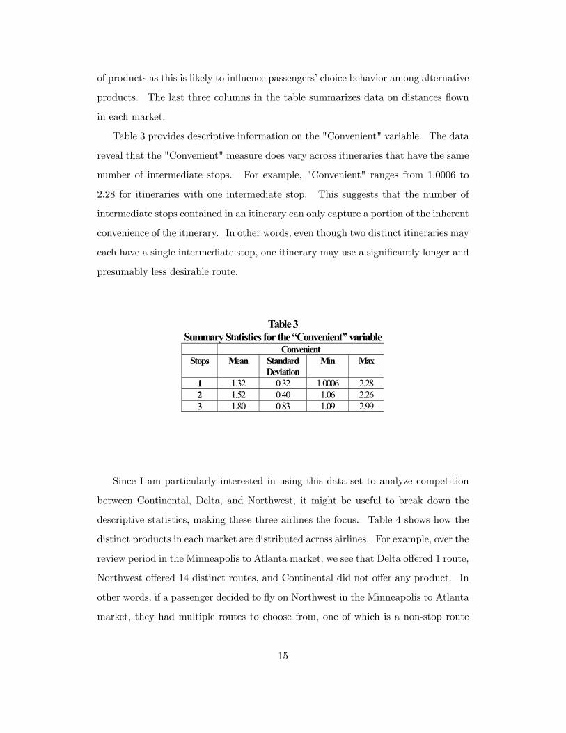
Table 3 provides descriptive information on the "Convenient" variable. The data

reveal that the "Convenient" measure does vary across itineraries that have the same

number of intermediate stops. For example, "Convenient" ranges from 1.0006 to

2.28 for itineraries with one intermediate stop. This suggests that the number of

intermediate stops contained in an itinerary can only capture a portion of the inherent

convenience of the itinerary. In other words, even though two distinct itineraries may

each have a single intermediate stop, one itinerary may use a significantly longer and

presumably less desirable route.

Table 3 Summary Statistics for the “Convenient” variable

Convenient Stops Mean Standard

Deviation Min Max

1 1.32 0.32 1.0006 2.28 2 1.52 0.40 1.06 2.26 3 1.80 0.83 1.09 2.99

Since I am particularly interested in using this data set to analyze competition

between Continental, Delta, and Northwest, it might be useful to break down the

descriptive statistics, making these three airlines the focus. Table 4 shows how the

distinct products in each market are distributed across airlines. For example, over the

review period in the Minneapolis to Atlanta market, we see that Delta offered 1 route,

Northwest offered 14 distinct routes, and Continental did not offer any product. In

other words, if a passenger decided to fly on Northwest in the Minneapolis to Atlanta

market, they had multiple routes to choose from, one of which is a non-stop route

15

also offered by Delta. There are 17 other distinct products in this market, which are

distinguished by either airlines, routing, or both.

Table 4 Disaggregated Sample of Products

Sample of online products distributed by Airlines

Market Total Sample of Online Products

Continental Delta Northwest Others

Atlanta – Dallas 11 0 4 1 6 Atlanta – Newark 9 1 2 2 4 Atlanta - Los Angeles 31 0 2 3 26 Atlanta - Salt Lake City 10 1 2 2 5 Cincinnati - Atlanta 7 0 6 1 0 Cincinnati - Los Angeles 4 0 1 0 3 Cincinnati - Salt Lake City 5 1 1 0 3 Dallas – Atlanta 18 0 3 0 15 Dallas – Cincinnati 4 0 2 0 2 Dallas – Newark 25 1 0 4 20 Houston - Cleveland 12 6 0 2 4 Houston – Newark 21 7 1 4 9 Minneapolis – Atlanta 32 0 1 14 17 Salt Lake City – Atlanta 16 1 4 1 10 Salt Lake City - Cincinnati 4 0 3 0 1

Even if we observe the three airlines offering a disproportionate number of prod-

ucts in a particular market, this information is not sufficient to draw inferences about

the degree of competition that exists between them. For example, even though we

observe Northwest offering 14 distinct products in the Minneapolis to Atlanta market,

the information in table 4 does not allow us to say whether a significant number of

passengers would rather choose Delta’s single product or one of the other 17 products

if Northwest increases its prices by 10%. The empirical model is design to explore

such competition issues. In fact, we ultimately want to use the empirical model

to predict the extent to which their prices will increase if the three airlines were to

jointly, rather than competitively, price their products.

Continental, Delta, and Northwest’s mean prices when they are independently

pricing their products are reported in table 5. For comparative purposes, market

means are also reported in the table. Interestingly, for the markets where at least two

16

of the three airlines offer products, their mean prices are rarely uniformly above the

market mean. For example, in the Atlanta to Los Angeles market where both Delta

and Northwest offer products, Delta’s mean fare is substantially above the market

mean, while Northwest’s mean fare is substantially below the market mean. This

general pattern suggests that the three airlines may not have been colluding in the

pre-alliance industry.

Table 5 Mean Prices

Mean Price of Partner Airlines before alliance

Market Mean Price (Market)

Continental Delta Northwest

Atlanta – Dallas 183.77 - 232.54 239.00 Atlanta – Newark 215.67 191.68 360.18 109.75 Atlanta - Los Angeles 240.87 - 547.92 181.88 Atlanta - Salt Lake City 160.16 124.50 170.33 123.39 Cincinnati - Atlanta 327.05 - 363.06 111.00 Cincinnati - Los Angeles 315.27 - 604.50 - Cincinnati - Salt Lake City 197.09 150.00 400.20 - Dallas – Atlanta 280.17 - 222.59 - Dallas – Cincinnati 271.26 - 307.17 - Dallas – Newark 294.97 689.58 - 347.77 Houston - Cleveland 208.29 280.70 - 106.38 Houston – Newark 224.27 321.07 517.00 119.55 Minneapolis – Atlanta 287.46 - 162.10 293.95 Salt Lake City – Atlanta 178.14 157.67 238.94 115.78 Salt Lake City - Cincinnati 121.53 - 126.35 -

Given that the ticket purchase data discussed above do not have passenger-specific

information, such as income or age, I use information on the distribution of demo-

graphic data in the origin city to account for taste heterogeneity in travel demand.

As such, estimating equation (2) requires supplementing the ticket purchase data

with demographic data drawn from the origin city’s population in each market.22

These demographic data are drawn from the 2001 and 2002 Current Population Sur-

vey (CPS) published by the U.S. Bureau of Labor Statistics. Tables 6A and 6B

summarize the demographic data in each origin city.

A random sample of one thousand individuals is drawn from each origin city’s

22This non-parametric approach to model consumer heterogeniety is explained in more detail inNevo(2000a).

17

population. From the samples drawn, we can see that there is some diversity within

each city. For example, while the majority of the sample between ages 21 and 40

have weekly income below $1,200, quite a few individuals in this age group earn above

$1,200 per week. Further, most individuals above the age of 60 have income below

$1,200 per week. When faced with the same set of options, it is likely that these dis-

tinct groups of potential passengers may make different product choices. One reason

is that they may have different tastes over prices and flight schedule convenience.

The empirical model is designed to account for such passenger heterogeneity.

Table 6A Summary of Demographic Data

Age Atl- anta

<21 21 to 30

31 to 40

41 to 50

51 to 60

61 to 70

71 to 80

>80 Total

Income < $300 27 37 25 21 10 5 2 0 127 $300 to $599 9 112 95 71 40 9 0 1 337 $600 to $899 2 79 64 65 43 6 1 0 260 $900 to $1199 0 34 50 31 22 1 1 0 139 $1200 to $1499 0 8 23 13 8 0 0 0 52 $1500 to $1799 0 7 11 10 8 0 0 0 36 $1800 or more 0 4 19 18 8 0 0 0 49 Total 38 281 287 229 139 21 4 1 1,000 Cinc- innati

Income < $300 26 51 26 21 23 10 8 1 166 $300 to $599 16 108 85 76 58 18 3 0 364 $600 to $899 3 35 71 70 48 6 1 0 234 $900 to $1199 0 10 36 43 23 5 0 0 117 $1200 to $1499 0 7 12 19 9 0 0 0 47 $1500 to $1799 0 2 9 10 9 0 0 0 30 $1800 or more 0 4 13 15 10 0 0 0 42 Total 45 217 252 254 180 39 12 1 1,000 Dallas Income < $300 36 49 39 27 6 5 1 1 164 $300 to $599 17 101 99 71 36 7 1 0 332 $600 to $899 3 66 69 50 31 4 0 0 223 $900 to $1199 0 22 42 21 20 5 1 0 111 $1200 to $1499 0 7 24 20 8 1 0 0 60 $1500 to $1799 0 4 11 16 5 0 0 0 36 $1800 or more 0 9 29 23 11 2 0 0 74 Total 56 258 313 228 117 24 3 1 1,000

Notes: The income variable is weekly income. Numbers in matrix refer to number of individuals in the income-age category.

18

Table 6B Summary of Demographic Data

Age Hous- ton

<21 21 to 30

31 to 40

41 to 50

51 to 60

61 to 70

71to 80

>80 Total

Income < $300 33 50 38 29 14 10 2 0 176 $300 to $599 17 122 103 83 42 13 1 0 381 $600 to $899 2 44 77 65 27 3 0 0 218 $900 to $1199 1 22 19 21 22 1 1 1 88 $1200 to $1499 0 13 22 25 4 0 0 1 65 $1500 to $1799 0 2 8 14 4 1 0 0 29 $1800 or more 0 4 3 23 10 3 0 0 43 Total 53 257 270 260 123 31 4 2 1,000 Minne- apolis

Income < $300 38 29 21 19 10 12 6 0 135 $300 to $599 13 87 63 69 22 8 5 1 268 $600 to $899 5 58 76 67 38 9 0 0 253 $900 to $1199 0 20 57 50 36 2 0 0 165 $1200 to $1499 0 11 25 24 14 4 0 0 78 $1500 to $1799 0 3 10 13 12 1 0 0 39 $1800 or more 0 1 19 27 13 2 0 0 62 Total 56 209 271 269 145 38 11 1 1,000 Salt Lake City

Income < $300 66 56 32 27 17 12 1 0 211 $300 to $599 25 116 81 61 42 18 1 2 346 $600 to $899 0 56 77 73 22 7 1 0 236 $900 to $1199 0 17 31 29 25 8 1 0 111 $1200 to $1499 0 3 18 12 11 2 0 0 46 $1500 to $1799 0 3 6 7 3 3 0 0 22 $1800 or more 0 3 7 7 5 6 0 0 28 Total 91 254 252 216 125 56 4 2 1,000

Notes: The income variable is weekly income. Numbers in matrix refer to number of individuals in the income-age category.

5 Results

In this section, I first interpret and discuss the estimates of the demand parameters.

I then use these estimates to compute own and cross price elasticities, and proceed to

discuss these elasticities with a particular focus on competition between Continental,

Delta, and Northwest in each market. The discussion on the elasticities serves as an

introduction to analyzing the supply side of the model, where I simulate the collusive

post-alliance equilibrium and quantify the extent to which these prices may differ

from their pre-alliance levels.

19

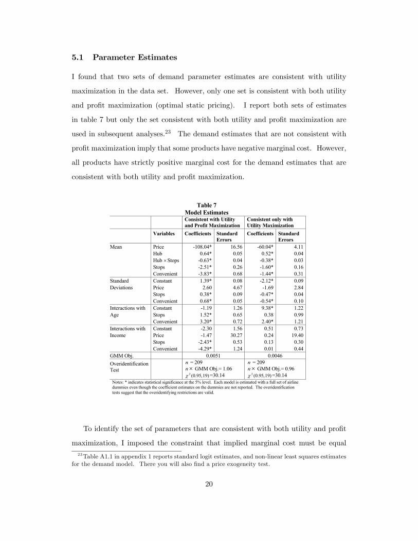
5.1 Parameter Estimates

I found that two sets of demand parameter estimates are consistent with utility

maximization in the data set. However, only one set is consistent with both utility

and profit maximization (optimal static pricing). I report both sets of estimates

in table 7 but only the set consistent with both utility and profit maximization are

used in subsequent analyses.23 The demand estimates that are not consistent with

profit maximization imply that some products have negative marginal cost. However,

all products have strictly positive marginal cost for the demand estimates that are

consistent with both utility and profit maximization.

Table 7 Model Estimates

Consistent with Utility and Profit Maximization

Consistent only with Utility Maximization

Variables

Coefficients

Standard Errors

Coefficients

Standard Errors

Mean Price -108.04* 16.56 -60.04* 4.11 Hub 0.64* 0.05 0.52* 0.04 Hub ×Stops -0.63* 0.04 -0.38* 0.03 Stops -2.51* 0.26 -1.60* 0.16 Convenient -3.83* 0.68 -1.44* 0.31 Standard Constant 1.39* 0.08 -2.12* 0.09 Deviations Price 2.60 4.67 -1.69 2.84 Stops 0.38* 0.09 -0.47* 0.04 Convenient 0.68* 0.05 -0.54* 0.10 Interactions with Constant -1.19 1.26 9.38* 1.22 Age Stops 1.52* 0.65 0.38 0.99 Convenient 3.20* 0.72 2.40* 1.21 Interactions with Constant -2.30 1.56 0.51 0.73 Income Price -1.47 30.27 0.24 19.40 Stops -2.43* 0.53 0.13 0.30 Convenient -4.29* 1.24 0.01 0.44 GMM Obj. 0.0051 0.0046 Overidentification Test

n = 209 n × GMM Obj.= 1.06

)19 ,95.0(2χ =30.14

n = 209 n × GMM Obj.= 0.96

)19 ,95.0(2χ =30.14 Notes: * indicates statistical significance at the 5% level. Each model is estimated with a full set of airline dummies even though the coefficient estimates on the dummies are not reported. The overidentification tests suggest that the overidentifying restrictions are valid.

To identify the set of parameters that are consistent with both utility and profit

maximization, I imposed the constraint that implied marginal cost must be equal23Table A1.1 in appendix 1 reports standard logit estimates, and non-linear least squares estimates

for the demand model. There you will also find a price exogeneity test.

20

to or greater than zero when minimizing the GMM objective function.24 In this

constrained minimization, the constraint is not binding at the solution parameters.

This therefore suggests that these solution parameters describe equilibrium consumer

behavior irrespective of the non-negative marginal cost constraint. As such, rather

than being a constraint, the non-negative marginal cost requirement serves more to

identify optimizing consumer behavior that is consistent with market equilibrium.

As expected, the coefficient on "Price" is negative, indicating that an airline

can increase the probability that potential passengers will choose it’s flight itinerary

by lowering the airfare on the said itinerary, ceteris paribus. It does not appear

that there is significant taste heterogeneity with respect to price since the standard

deviation of the price effect and the coefficient on the interaction of price with income

are not statistically different from zero at conventional levels of significance.

Two possible reasons why passengers are more likely to choose itineraries offered

by hub airlines are: (1) flight schedules offered by hub airlines may be more conve-

nient, (2) it is more likely that passengers have frequent flyer membership with a hub

airline.25 The variable "Hub" is a dummy variable taking the value one if the prod-

uct is offered by an airline that has a hub at the origin airport and zero otherwise.

The coefficient on "Hub" is positive, indicating that potential passengers are more

likely to choose itineraries where the origin airport is a hub for the airline offering the

itinerary. In other words, airlines have a strategic advantage at their hub airports

compared to their non-hub competitors.

Another product characteristic that influences passengers’ choice of products is

the convenience of flight schedule embodied in the itinerary. I use number of inter-

mediate stops on an itinerary to capture a portion of this convenience effect. The

coefficient on this variable has a negative sign as expected and is statistically signif-

icant at conventional levels of significance. This indicates that consumers are more

likely to choose flight itineraries with less intermediate stops, ceteris paribus. The

24The inequality constraint is formulated as p−£− (Ω ∗4)−1 s(p)¤ ≥ 0, where £− (Ω ∗4)−1 s(p)¤is the markup function that is nonlinear in the demand parameters.25See Proussaloglou and Koppelman (1995), Berry (1990), Schumann (1986).

21

coefficient on the interaction between number of intermediate stops and "Hub" is neg-

ative as expected, and statistically significant at conventional levels of significance.

The negative coefficient on this interaction variable suggests that the attractiveness

of hub products over their non-hub counterparts is lessened as the number of inter-

mediate stops in hub products’ itinerary increases, ceteris paribus. In addition, the

marginal disutility of an intermediate stop is greater for hub products compared to

non-hub products. This could be suggesting that passengers expect hub products

to have convenient schedules and thus they are more heavily penalized relative to

non-hub products for not having convenient schedules.

It appears that passengers’ have heterogenous taste with respect to the num-

ber of intermediate stops as evidenced by the statistical significance of the standard

deviation parameter for "Stops". Further, a negative coefficient when "Stops" is in-

teracted with income suggests that higher income passengers are more likely to choose

itineraries with less intermediate stops compared to lower income passengers. The

positive coefficient when "Stops" is interacted with age suggests older passengers are

more likely to choose itineraries with more intermediate stops compared to younger

passengers. It could be that older passengers tend to be more leisure travelers and

therefore care less about itinerary convenience relative to younger passengers. In

summary, young high-income passengers seem to care more about number of inter-

mediate stops relative to old low-income passengers.

Recognizing that number of intermediate stops may only capture a portion of

the inherent convenience of an itinerary, I also included the "Convenient" variable.

Recall that "Convenient" is the ratio of itinerary distance to the non-stop distance

between the origin and destination cities. This variable is able to distinguish between

various routes that have the same number of intermediate stops but differ with respect

to distance flown in getting the passenger from the origin to destination city. As

expected, the coefficient on "Convenient" has a negative sign and is statistically

different from zero. In other words, passengers prefer to use a less circuitous route

in traveling from the origin to destination city.

22

The statistical significance of the standard deviation parameter for "Convenient"

suggests that passengers are heterogenous with respect to their taste for the distance

of the route used in traveling from the origin to destination city. Further, the sign

pattern of the coefficients when "Convenient" is interacted with income and age

suggests that younger, higher income passengers are relatively more concerned with

itinerary convenience. This qualitative result coincides with these young high-income

passengers’ taste for number of intermediate stops discussed above.

5.1.1 Elasticities

In analyzing the degree of competition that exists between Continental, Delta, and

Northwest in each market, I first use the demand parameter estimates to construct

matrices of own and cross prices elasticities of demand.26 Each market has its own

elasticity matrix associated with it. The entries on the main diagonal of each matrix

are estimates of the airlines’ average own price elasticity of demand, while off diagonal

elements are estimates of the airlines’ average cross price elasticities of demand. An

element in the matrix is interpreted as the percentage by which a row airline’s demand

changes as a result of a change in the price of a column airline.

The elasticity matrix for the Atlanta-Dallas market is presented in table 8 while,

the matrices for the other markets are located in appendix 2. The estimates in table

8 suggest that a 1% increase in Delta’s price will reduce quantity demand for Delta’s

products by 2.48%. Similarly, a 1% increase in Northwest’s price will reduce quantity

demand for Northwest’s products by 2.54%. However, cross elasticity estimates

suggest that a 1% increase in Delta’s price will increase Northwest’s demand by

0.0027%, while a 1% increase in Northwest’s price will increase Delta’s demand by

0.0004%.

26See Nevo (2000a) for details on how own and cross price elasticities are computed in the case ofthe random coefficients logit model.

23

Table 8 Price Elasticity of Demand Matrix

Market: Atlanta – Dallas TZ DL FL NJ NW UA TZ -1.4949 0.0018 0.0592 0.0013 0.0004 0.0088 DL 0.0270 -2.4809 0.0642 0.0016 0.0004 0.0109 FL 0.0194 0.0014 -1.3605 0.0008 0.0002 0.0045 NJ 0.0256 0.0019 0.0611 -1.2764 0.0004 0.0099 NW 0.0354 0.0027 0.0831 0.0029 -2.5437 0.0229 UA 0.0344 0.0026 0.0812 0.0026 0.0009 -2.0903 Outside 0.0011 0.0001 0.0027 0.00003 0.00001 0.0001

Recall that the outside good represents travel options in the given market that

are not explicitly included in the model. For example, the outside good includes

air travel products that involve multiple airlines, and other means of getting from

the origin to destination city besides air travel. An element in the last row of the

matrix tells us by how much the demand for the outside good changes as a result of a

change in the price of the column airline. For example, a 1% increase in Delta’s price

increases demand for the outside good by 0.0001%, while a 1% increase in Northwest’s

price increase the demand for the outside good by 0.00001%.

While interpretation of the own and cross price elasticities of demand is a useful

exercise to see how sensitive the demand is for an airline’s products to changes in its

own or other airlines’ prices, we ultimately want to derive a comparative measure of

the degree of competition between competing airlines. Such a measure is obtained

by weighting the elasticities by their respective quantities and dividing an airline’s

quantity-weighted cross price elasticity by its quantity-weighted own price elasticity.

This ratio tells us the proportion of an airline’s lost sales that is captured by a

competitor. For example, suppose airlines A, B, and C compete in a market. Let ηaa,

ηba, and ηca be the own, and cross price elasticities for airline A, where ηaa =∂Qa

∂PaPaQa,

ηba =∂Qb∂Pa

PaQb, and ηca =

∂Qc

∂PaPaQcrespectively. That is, ηaa, ηba, and ηca tell us how

airline A, B, and C, sales are affected by a change in airline A’s price. However, the

24

ratio ηba×Qb

ηaa×Qatells us the proportion of airline A’s lost sales that is captured by airline

B if airline A increases its price marginally. Likewise, ηca×Qc

ηaa×Qatells us the proportion

of airline A’s lost sales that is captured by airline C if airline A increases its price

marginally. Therefore, if ηba×Qb

ηaa×Qa> ηca×Qc

ηaa×Qa, we can infer that airline B is a closer

competitor to airline A than is airline C to airline A.

These comparative measures of the closeness of competitors are computed and

presented in tables 9A, 9B, and 9C. An entry in these tables tells us, on average,27 the

percentage of the column airline’s lost sales that is captured by the row airline given a

marginal increase in the column airline’s price. Each column gives a complete break

down of how the column airline’s lost sales are distributed and therefore sums to 100.

The tables are constructed with a focus on competition between Delta, Continental,

and Northwest in each market. As such, entries in the row labeled "Inside" is an

aggregate across the products of the other airlines included in the model. As before,

the row labeled "Outside" represents the composite outside option.

Table 9A Percentage of lost sales going to competing products

Atlanta – Dallas Atlanta – Newark

Atlanta - Los Angeles

Atlanta - Salt Lake City

Airlines DL NW CO DL NW DL NW CO DL NW CO - - - 0.29 0.31 - - - 0.02 0.02 DL 0.35 0.58 0.13 0.04 0.12 0.03 0.05 0.01 0.01 0.01 NW 0.02 - 0.09 0.11 0.06 0.42 0.26 0.91 0.64 0.26 Inside 8.37 11.48 5.38 4.54 4.92 15.55 14.74 1.64 1.13 1.25 Outside 91.27 87.94 94.41 95.03 94.59 84.01 84.94 97.43 98.21 98.46 Total 100 100 100 100 100 100 100 100 100 100

27Since some airlines may offer multiple products within a market, for these airlines, an entry inthe table is an average across the products offered by the airline.

25

Table 9B Percentage of lost sales going to competing products

Cincinnati – Atlanta

Cincinnati - Los Angeles

Cincinnati - Salt Lake City

Dallas – Atlanta

Dallas – Cincinnati

Dallas – Newark

Airlines DL NW DL CO DL DL DL CO NW CO - - - - 0.01 - - - 0.03 DL 0.29 0.37 - 0.05 - 0.02 0.05 - - NW 0.04 - - - - - - 0.05 0.05 Inside - - 0.98 0.07 0.05 1.31 0.05 2.97 3.78 Outside 99.67 99.63 99.02 99.88 99.94 98.66 99.91 96.98 96.14 Total 100 100 100 100 100 100 100 100 100

Table 9C Percentage of lost sales going to competing products

Houston – Cleveland Houston – Newark

Minneapolis – Atlanta

Salt Lake City – Atlanta

Salt Lake City – Cincinnati

Airlines CO NW CO DL NW DL NW CO DL NW DL CO 0.03 0.04 0.04 0.05 0.04 - - - 0.10 0.08 - DL - - 0.001 - 0.001 - 0.13 0.29 0.27 0.30 0.09 NW 0.02 0.01 0.06 0.06 0.04 7.72 13.30 3.33 4.28 - - Inside 0.06 0.07 0.34 0.33 0.32 1.60 3.42 9.11 11.66 9.47 0.46 Outside 99.89 99.88 99.57 99.57 99.59 90.68 83.14 87.27 83.70 90.15 99.45 Total 100 100 100 100 100 100 100 100 100 100 100

In the Atlanta to Dallas market we see that Northwest only captures 0.02% of

Delta’s lost sales when Delta increases its price marginally. In contrast, online

products offered by other airlines in this market manage to capture 8.37% of Delta’s

lost sales, while 91.27% goes to the outside option. For completeness in describing

the entries in the column, I ought to describe Delta’s ability to recapture some of its

lost sales. That is, since Delta is a multiproduct firm in this market, whenever it

increases its price marginally on one of its products, on average, its other substitute

products recapture 0.35% of the lost sales from the product whose price increased

marginally.

The second column in the Atlanta to Dallas market tells us that Delta is only able

to capture 0.58% of Northwest’s lost sales if Northwest increases its price marginally,

26

while the other inside products and the outside option capture 11.48% and 87.94%

of Northwest’s lost sales respectively. The data therefore suggest that competition

between Delta and Northwest is relatively weak in the Atlanta to Dallas market. In

fact, the only market where competition seems meaningful between Delta and North-

west is the Minneapolis to Atlanta market. In this market we see that Northwest has

the ability to capture 7.72% of Delta’s lost sales if Delta increases its price marginally.

In summary, competition between the three airlines seems weak. This suggests

that equilibrium prices for these airlines should not be expected to change much if

they jointly, as oppose to noncooperatively, price their products. In other words,

passengers seem to have sufficiently attractive travel alternatives in these markets

that would effectively constrain collusive behavior between Delta, Continental, and

Northwest. However, without incorporating the supply side of the model in the

analysis, we cannot predict by how much equilibrium prices may change in moving

from a noncooperative to a collusive equilibrium.

5.1.2 Sensitivity Analysis

Before moving on to discuss the supply side results, it is prudent to analyze how

sensitive the previous results are to changes in the definition of market size.28 As

a reminder, market size (M) is assume to be equal to the size of the population in

the origin city. To perform the sensitivity analysis, I re-estimate the model under

two different market size definitions: (1) market size equal to 15% of origin city

population; (2) market size equal to twice the size of origin city population. I then

re-compute the matrices in tables 9A, 9B, and 9C under each market size definition.

These new matrices, 9A-1, 9B-1, 9C-1, 9A-2, 9B-2, and 9C-2, are located in appendix

2.

The outside option becomes a closer substitute to all products included in the

model, the larger the potential market. In other words, by defining the market

size as twice the origin city population instead of 15% of or equal to the origin city

28 I thank an anonymous referee for suggesting that I do this.

27

population, we make the potential market larger and effectively make the outside

option a closer substitute for all included products. Therefore, as expected, the

matrices in tables 9A-1, 9B-1, and 9C-1 reveal that when market size is defined as

15% of origin city population, the amount of the airlines’ lost sales going to the outside

option is lower in most cases. The converse holds when the market size is defined as

twice the origin city population. However, as is the case in tables 9A, 9B, and 9C,

a relatively large proportion of lost sales still goes to the outside option irrespective

of substantial variation in the definition of market size. Since we would not expect

a substantial number of people to choose not to fly if the concerned airlines increase

their price marginally, then the outside option is likely picking up air travel products

not captured in the data. These excluded air travel products will likely further

thwart effective collusive behavior by the three airlines. This inference is supported

by the fact that substitutability between the three airlines remains relatively low

irrespective of the market size definition as evidenced in the recomputed matrices.

Subsequent analyses are based on market size being equal to origin city popula-

tion. However, qualitative results are robust to wide variations in market definition.

5.2 Supply and Equilibrium

Table 10 reports the predicted effects of Delta, Continental, and Northwest jointly as

oppose to noncooperatively pricing their products. Tables A 3.1 and A 3.2, located

in appendix 3, present similar price comparisons for other competing airlines in each

market. The first data column in the table shows the three airlines’ median pre-

alliance prices in each market. The second data column shows the median percent by

which each of the three airlines’ price will increase if they jointly price their products

in the post-alliance industry, ceteris paribus. Consistent with our analyses of the

demand elasticities in the previous section, the only market where prices are expected

to increase is the Minneapolis to Atlanta market. Furthermore, the largest median

price increase is only 4.44%. These findings further confirm that passengers seem to

have sufficiently attractive travel alternatives in these markets that would effectively

28

constrain collusive behavior between the three airlines.

Table 10 Predicted Effects of Joint Pricing

Market

Airline

MedianPrice

Median Percent Price Increase

Median Marginal Cost

Median Marginal Cost Reduction

Atlanta – Dallas Delta 219.00 0 124.81 0 Northwest 239.00 0 145.04 0 Atlanta – Newark Continental 191.68 0 97.91 0 Delta 360.18 0 266.62 0 Northwest 109.75 0 16.31 0 Atlanta - Los Angeles Delta 547.92 0 453.86 0 Northwest 180.60 0 86.24 0 Atlanta - Salt Lake City Continental 124.50 0 31.66 0 Delta 170.33 0 77.19 0 Northwest 123.39 0 29.70 0 Cincinnati – Atlanta Delta 276.69 0 182.69 0 Northwest 111.00 0 17.04 0 Cincinnati - Salt Lake City Continental 150.00 0 56.90 0 Delta 400.20 0 306.95 0 Dallas – Newark Continental 689.58 0 596.27 0 Northwest 226.89 0 133.72 0 Houston – Cleveland Continental 232.59 0 139.73 0 Northwest 106.38 0 13.02 0 Houston – Newark Continental 224.60 0 130.97 0 Delta 517.00 0 423.25 0 Northwest 120.60 0 26.93 0 Minneapolis – Atlanta Delta 162.10 4.447 68.83 11.359 Northwest 191.44 0.063 86.58 0.163 Salt Lake City – Atlanta Continental 157.67 0 64.06 0 Delta 209.39 0 115.68 0 Northwest 115.78 0 19.02 0

Notes: The second data column shows the median percentage by which Delta, Continental, and Northwest’s predicted collusive prices exceed their actual prices. The third data column shows the median implied marginal cost for each of the three airlines in respective markets. The last data column shows the median percent by which marginal cost must fall to prevent price from increasing if the three airlines practice price collusion.

Since alliance partners often jointly use each others facilities (lounges, gates,

check-in counters etc.), and may also practice joint purchase of fuel, it is likely that

alliances generate cost saving. As such, an interesting question to pose is: How much

29

does marginal cost have to fall (extent of cost savings) in order to ensure that prices

do not change in the event that the three airlines jointly price their products?29 It

is important that policy makers have an impartial assessment of such cost savings

before making a decision on whether to approve a propose alliance. The policy mak-

ers can then compare their impartial assessment of required cost savings with the

cost savings and other benefits that the airlines will present to persuade approval.

The last column in table 10 provides these required cost savings estimates. Not

surprisingly, the only market where a reduction in marginal cost is necessary is the

Minneapolis to Atlanta market. The largest median marginal cost reduction required

is only 11.36%.

5.2.1 The Bertrand-Nash Assumption

A legitimate concern with the supply side analysis above is whether the Bertrand-

Nash assumption is reasonable in the case of the airline industry.30 To explore this

concern, I parameterize marginal cost using a popular functional form for marginal

cost in the empirical industrial organization literature,31

cjt = exp(Wjtγ + bj + ψjt), (6)

where γ is a vector of parameters to be estimated,Wjt is a vector of variables that shift

marginal cost, bj are product fixed effects (airline dummies) capturing the components

of an airline’s products’ marginal cost that are the same across markets, and ψjt is

a mean zero, random error term that captures unobserved determinants of marginal

cost.

The Bertrand-Nash assumption results in the following supply equation,

pjt = exp(Wjtγ + bj + ψjt)+mjt, (7)

29 I thank an anonymous referee for pointing out this important policy relevant cost analysis.30 I thank the editor, Dennis Carlton, for suggesting that I explore the appropriateness of the

Bertrand-Nash assumption.31For example, see Goldberg and Verboven (2001), and Ivaldi and Verboven (2004).

30

where mjt is a markup variable that is computed prior to econometrically estimating

the supply equation.32 By transforming equation (7) as follows,

ln (pjt −mjt) =Wjtγ + bj + ψjt, (8)

we can use simple linear estimation techniques to estimate the parameters of the

marginal cost function. These parameter estimates are reported in table 11.33

Table 11 Marginal Cost Function Parameter Estimates

Variables Coefficient Estimates Standard Error Hub 0.26 0.19 Itinerary Distance 2.44* 0.75 (Itinerary Distance)2 -0.56* 0.20 R2 0.97 Notes: * indicates statistical significance at the 5% level. The coefficients are estimated using ordinary least squares. A full set of airline and market dummies are included when estimating the model, even though these parameter estimates are not reported.

While the coefficient on "Hub" is not statistically different from zero at conven-

tional levels of significance, the other coefficients suggest that marginal cost has an

inverted U-relationship with itinerary distance. This finding is consistent with an

argument made in Berry, Carnal, and Spiller (1997) which says that at relatively

short distances the superior cruising efficiency of larger planes may not dominate

their larger takeoff and landing cost and therefore marginal cost is increasing in dis-

tance at relatively short distances. However, at relatively long distances it becomes

32With estimates of the demand parameters in hand, the markup variable is computed using− (Ω ∗4)−1 s(p).33Technically, the standard errors of the supply parameters should be corrected to reflect the fact

that mjt is a function of previously estimated demand parameters [see Newey and McFadden (1994)].However, this correction is complicated to implement because mjt is highly nonlinear in the demandparameters. Since the method used below to evaluate the appropriateness of the Bertrand-Nashassumption, which is the main objective of this subsection, does not require corrected standard errors,I just report the uncorrected standard errors in table 11. As such, we must exercise caution whendrawing conclusions from table 11 about the determinants of marginal cost.

31

optimal to use larger planes since their cruising efficiency may dominate their higher

takeoff and landing cost which eventually cause marginal cost to decline in distance.

With estimates of the marginal cost parameters in hand, we can first compute

estimates of marginal cost, bcjt = exp(Wjtbγ+bbj), and then use these estimates to solvefor the prices that satisfy equation (4), s(p)+(Ω∗∆) (p− bc) = 0. If these predictedBertrand-Nash prices are not highly correlated with actual prices, then either the

functional form assumption for marginal cost is inappropriate or the Bertrand-Nash

assumption is inappropriate, or both.34 However, I found that predicted Bertrand-

Nash and actual prices are highly correlated (correlation of 0.90) which suggests that

the Bertrand-Nash assumption may be reasonable. This is also illustrated graphically

in figures 1 to 4 where I plot the actual and predicted Bertrand-Nash price series.

We can see that the model does a good job at predicting actual prices.

Figure 1: Products in Markets 1 - 3

0200400600800

1000

1 4 7 10 13 16 19 22 25 28 31 34 37 40 43 46 49

Products

Pric

es

Actual Price Predicted Bertrand-Nash Price

34 I thank an anonymous referee for pointing out that a comparison between actual prices and thepredicted Bertrand-Nash prices is basically a joint test of the marginal cost specification and theBertrand-Nash assumption.

32

Figure 2: Products in Markets 4 - 9

0

200400

600800

1000

1 3 5 7 9 11 13 15 17 19 21 23 25 27 29 31 33 35 37 39 41 43 45 47

ProductsPr

ices

Actual Price Predicted Bertrand-Nash Price

Figure 3: Products in Markets 10 - 12

0

500

1000

1500

1 4 7 10 13 16 19 22 25 28 31 34 37 40 43 46 49 52 55 58

Products

Pric

es

Actual Price Predicted Bertrand-Nash Price

Figure 4: Products in Markets 13 - 15

0200400600800

10001200

1 4 7 10 13 16 19 22 25 28 31 34 37 40 43 46 49 52

Products

Pric

es

Actual Price Predicted Bertrand-Nash Price

33

5.2.2 Reconciling Predictions with Reality

In June 2003, Continental, Delta, and Northwest, launched their alliance after satis-

fying policy makers that they would remain competitive on overlapping routes rather

than practice collusion. Recall that any predicted price increase in table 10, is based

on the assumptions that, (1) alliance partners’ collude on prices, (2) there were no cost

efficiencies generated by the alliance. In other words, if alliance partners continue to

compete as in the pre-alliance industry, and if the alliance generated cost efficiencies,

then prices may even fall on overlapping routes in the post-alliance industry.

An extremely crude check of how prices actually changed is presented in table 12.

The data in table 12 represent percent change in median prices by airline between the

first quarter of 2002 (pre-alliance and sample period), and the first quarter of 2004

(post-alliance period). The reason these percentages are extremely crude checks of

how prices actually changed is that the Origin and Destination Survey data is a 10%

sample of tickets sold in respective quarters. As such, there is no guarantee that

sampled products will correspond across quarters and therefore I am left with little

choice but to compare each airlines’ median prices across quarters. For example, the

data for one quarter may contain an itinerary which has a passenger flying on Delta,

from Atlanta to Newark with an intermediate stop in Chicago, but this itinerary may

not be present in subsequent quarters.

Table 12 Actual Percentage Change in Median Price

Market Continental Delta Northwest Atlanta – Dallas -12.3 -54.2 Atlanta – Newark -8.2 -45.0 6.6 Atlanta - Los Angeles -55.1 36.9 Atlanta - Salt Lake City -8.0 46.3 5.3 Dallas – Newark -35.1 -55.1 Houston – Cleveland -19.9 26.7 Houston – Newark -12.5 -45.0 -4.9 Minneapolis – Atlanta 19.8 -37.4 Salt Lake City – Atlanta -24.1 18.0 0.4 Notes: The numbers in the table refer to percentage change in median price between the first quarter of 2002 and the first quarter of 2004. The subset of markets shown above are markets in which at least two of the partners competed in the pre-alliance market (first quarter of 2002) and continue to offer products in the post-alliance market (first quarter of 2004).

34

Notwithstanding the limitations of the data, the actual percent change in prices

shown in table 12 reveal an interesting result. In the majority of cases, the alliance

partners median prices actually fell in the post-alliance period.35 This suggests

that either the alliance partners kept their promise not to collude on prices, or the

alliance generated sufficient cost savings36 which resulted in lower prices, or both. In

summary, both the post-alliance data and the results from the model seem to suggest

that policy makers’ ultimate approval of the alliance appeared justified.

6 Conclusion

The main contribution of this paper is to show how policy makers can use a structural

econometric framework developed by Nevo (2000b) to quantify the competitive effects

of proposed code-share alliances, where potential alliance partners compete on over-

lapping routes in the pre-alliance industry. Specifically, the framework can be used

to quantify the extent to which collusive prices may depart from their pre-alliance

levels in the worst case scenario where there is no commensurate generation of cost

efficiency by the alliance. Furthermore, it can also be used to compute the extent to

which marginal cost must fall in order for prices to remain unchanged in the event

that partners do collude on prices in the post-alliance industry. In seeking approval

from policy makers, potential alliance partners have an incentive to emphasize the

benefits of the proposed alliance. Using this structural framework, policy makers can

reconcile the alleged benefits with potential price increases, allowing them to make

an informed decision regarding approval.

As an example, I applied the structural model to the proposed Continental/

Delta/ Northwest alliance. In reviewing the proposed alliance, the DOT raised con-

35Had the percentages in the table been adjusted for inflation, then the price increases would beeven smaller.36Chua, Kew, and Yong(2003) present an interesting empirical analysis of the effect of code-share

alliances on partners’ cost. They found that code-share alliances reduce airlines’ cost, albeit smallin magnitude.

35

cerns regarding the significant overlap in the potential partners’ route network. In

the sample of markets that were examined, I did not find any significant departure

between collusive and pre-alliance prices. This suggests that passengers have suffi-

ciently attractive travel alternatives in these markets that would effectively constrain

collusive behavior between the three airlines.

With the potential partners’ representation that they would not collude on prices

along with satisfying other conditions,37 the DOT ultimately allowed the alliance to

go through. A crude comparison of the airlines’ prices before and after formation of

the alliance revealed that their prices actually fell in most of the markets considered

in the analysis. Thus, both the model’s predictions and the actual post-alliance

prices suggest that policy makers’ approval appears justified.

37See “Termination of Review Under 49 U.S.C § 41720 of Delta/Northwest/Continental Agree-ments,” Department of Transportation, Office of The Secretary, January 2003.

36

A Appendix 1.

Table A1.1 Demand Estimates

Variables

(3) OLS

(4) 2SLS

(5) NNLS

Mean Price

-21.68** (7.31)

-72.34** (18.87)

-29.72 (67.75)

Hub

0.31 (0.49)

0.64 (0.56)

0.10 (0.50)

Hub ×Stops

-0.41 (0.34)

-0.44 (0.38)

-0.60* (0.36)

Stops

-1.28** (0.23)

-1.19** (0.26)

-2.68* (1.51)

Convenient

-1.03** (0.36)

-0.71* (0.42)

-4.25 (4.23)

Constant

1.42* (0.75)

Standard Deviations

Price

2.23 (29.07)

Stops

0.36 (0.74)

Convenient

0.60 (0.48)

Constant

-1.01 (8.78)

Interactions with Age

Stops

1.52 (3.82)

Convenient

2.92 (5.36)

Constant

-2.43 (7.97)

Interactions with Income

Price

-1.95 (116.58)

Stops

-2.44 (2.95)

Convenient

-4.43 (7.10)

R2

0.98

Model Diagnostics

Price Exogeneity Test Statistic )1 ,95.0(2χ

8.48 3.84

Notes: ** indicates statistical significance at the 5% level. * indicates statistical significance at the 10% level. Standard errors are in parentheses. All models are estimated with a full set of airline dummies even though the coefficient estimates on the dummies are not reported. The dependent variable for columns (3) and (4) is )ln()ln( 0tjt ss − . The Nonlinear Least Squares (NLLS) estimates

in column (5) are obtained without using any instrument for price. The price exogeneity test suggests that price is endogenous and needs to be instrumented for.

B Appendix 2.

37

Price Elasticity of Demand Matrix Market: Atlanta – Newark AA CO DL FL NW US AA -3.1079 0.0059 0.0013 0.0565 0.0007 0.0030 CO 0.0005 -2.0440 0.0013 0.0671 0.0005 0.0026 DL 0.0007 0.0059 -3.8526 0.0556 0.0007 0.0028 FL 0.0005 0.0071 0.0013 -1.2530 0.0005 0.0026 NW 0.0008 0.0063 0.0013 0.0603 -1.1752 0.0031 US 0.0007 0.0071 0.0014 0.0671 0.0007 -1.1291 Outside 0.00002 0.0003 0.0001 0.0026 0.00002 0.0001

Price Elasticity of Demand Matrix Market: Atlanta - Los Angeles

AA DL F9 HP NJ NW UA US YX AA -2.556 0.0015 0.0122 0.0127 0.0361 0.0025 0.0076 0.0106 0.0002 DL 0.0060 -5.8369 0.0133 0.0136 0.0388 0.0028 0.0082 0.0119 0.0003 F9 0.0046 0.0013 -2.8234 0.0108 0.0299 0.0020 0.0061 0.0083 0.0002 HP 0.0058 0.0015 0.0123 -2.0621 0.0373 0.0027 0.0079 0.0112 0.0002 NJ 0.0045 0.0013 0.0106 0.0108 -2.1468 0.0020 0.0060 0.0082 0.0002 NW 0.0057 0.0015 0.0127 0.0131 0.0371 -1.9375 0.0078 0.0110 0.0002 UA 0.0061 0.0016 0.0131 0.0137 0.0392 0.0028 -2.8997 0.0119 0.0003 US 0.0066 0.0018 0.0142 0.0148 0.0423 0.0030 0.0090 -1.5570 0.0003 YX 0.0059 0.0016 0.0130 0.0135 0.0382 0.0027 0.0081 0.0114 -1.3590 Outside 0.0002 0.0001 0.0004 0.0004 0.0011 0.0001 0.0002 0.0002 0.00001

Price Elasticity of Demand Matrix Market: Atlanta - Salt Lake City AA CO DL F9 HP NW UA AA -1.8467 0.0003 0.0001 0.0042 0.0133 0.0053 0.0075 CO 0.0009 -1.3411 0.0001 0.0044 0.0141 0.0056 0.0079 DL 0.0006 0.0002 -1.8291 0.0031 0.0094 0.0039 0.0056 F9 0.0008 0.0003 0.0001 -2.6554 0.0117 0.0048 0.0068 HP 0.0010 0.0004 0.0001 0.0047 -1.5960 0.0061 0.0085 NW 0.0007 0.0003 0.0001 0.0034 0.0105 -1.3205 0.0061 UA 0.0008 0.0003 0.0001 0.0039 0.0121 0.0049 -1.6008 Outside 0.00004 0.00001 0.00001 0.0002 0.0005 0.0002 0.0003

38

Price Elasticity of Demand Matrix Market: Cincinnati – Atlanta DL NW DL -3.86105 0.000463NW 0.00209 -1.18139Outside 0.00003 0.000004

Price Elasticity of Demand Matrix Market: Cincinnati - Los Angeles AA DL UA AA -1.3054 0.0096 0.0157DL 0.0010 -6.3843 0.0142UA 0.0011 0.0089 -2.8329Outside 0.00002 0.0002 0.0002

Price Elasticity of Demand Matrix

Market: Cincinnati - Salt

Lake City AA CO DL UA AA -1.7516 0.0002 0.0021 0.0003CO 0.0003 -1.6112 0.0023 0.0004DL 0.0002 0.0001 -4.2916 0.0003UA 0.0002 0.0001 0.0020 -1.1738Outside 0.00001 0.000005 0.0001 0.00001

Price Elasticity of Demand Matrix Market: Dallas – Atlanta AA DL FL NJ UA YX AA -2.9999 0.0002 0.0024 0.0005 0.0006 0.0001 DL 0.0009 -2.3814 0.0031 0.0004 0.0006 0.0001 FL 0.0008 0.0002 -3.1621 0.0006 0.0009 0.0002 NJ 0.0009 0.0003 0.0026 -1.5361 0.0006 0.0001 UA 0.0009 0.0003 0.0027 0.0005 -1.3083 0.0001 YX 0.0009 0.0003 0.0026 0.0005 0.0007 -7.1524 Outside 0.00005 0.00001 0.0001 0.00002 0.00002 0.000004

39

Price Elasticity of Demand Matrix Market: Dallas – Cincinnati

AA DL UA AA -3.3954 0.0013 0.0004DL 0.0004 -3.2986 0.0006UA 0.0004 0.0017 -1.6600Outside 0.00002 0.0001 0.00002

Price Elasticity of Demand Matrix Market: Dallas – Newark AA CO FL NW UA US TZ YX AA -3.5423 0.0021 0.0093 0.0007 0.0019 0.0028 0.0082 0.0002CO 0.0058 -7.3901 0.0055 0.0004 0.0011 0.0017 0.0051 0.0001FL 0.0076 0.0020 -2.1114 0.0006 0.0016 0.0024 0.0072 0.0001NW 0.0071 0.0019 0.0075 -3.7282 0.0015 0.0023 0.0067 0.0001UA 0.0067 0.0018 0.0068 0.0005 -2.0160 0.0021 0.0062 0.0001US 0.0075 0.0020 0.0078 0.0005 0.0016 -1.1747 0.0071 0.0001TZ 0.0067 0.0018 0.0068 0.0005 0.0014 0.0021 -1.7261 0.0001YX 0.0076 0.0020 0.0081 0.0006 0.0016 0.0024 0.0073 -2.2169Outside 0.0002 0.00005 0.0001 0.00001 0.00003 0.00004 0.0001 0.000002

Price Elasticity of Demand Matrix Market: Houston – Cleveland AA CO NW UA US AA -1.7962 0.0002 0.0001 0.0003 0.0004 CO 0.0001 -3.0171 0.0001 0.0003 0.0004 NW 0.0001 0.0002 -1.1396 0.0003 0.0004 UA 0.0001 0.0002 0.0001 -1.5825 0.0004 US 0.0001 0.0002 0.0001 0.0003 -1.2868 Outside 0.00001 0.00001 0.000004 0.00001 0.00002

Price Elasticity of Demand Matrix Market: Houston – Newark AA CO DL NW UA US AA -2.2286 0.0003 0.0001 0.0002 0.0005 0.0008 CO 0.0005 -3.4254 0.0001 0.0002 0.0005 0.0008 DL 0.0005 0.0003 -5.5149 0.0002 0.0005 0.0008 NW 0.0005 0.0003 0.0001 -1.2779 0.0004 0.0007 UA 0.0005 0.0003 0.0001 0.0002 -1.6216 0.0008 US 0.0005 0.0003 0.0001 0.0002 0.0005 -1.3687 Outside 0.00002 0.00001 0.000003 0.00001 0.00002 0.00003

40

Price Elasticity of Demand Matrix Market: Minneapolis – Atlanta AA DL FL NW UA US AA -3.1100 0.0019 0.0029 0.0169 0.0032 0.0022 DL 0.0011 -1.7381 0.0017 0.0112 0.0016 0.0010 FL 0.0031 0.0025 -3.2433 0.0215 0.0045 0.0033 NW 0.0029 0.0023 0.0036 -3.1441 0.0042 0.0029 UA 0.0015 0.0016 0.0022 0.0137 -3.2128 0.0015 US 0.0026 0.0022 0.0033 0.0191 0.0037 -1.4185 Outside 0.0001 0.0001 0.0001 0.0008 0.0001 0.00004

Price Elasticity of Demand Matrix Market: Salt Lake City – Atlanta AA CO DL F9 HP NW UA AA -1.7025 0.0012 0.0016 0.0133 0.0280 0.0366 0.0108 CO 0.0073 -1.6843 0.0017 0.0146 0.0319 0.0412 0.0120 DL 0.0092 0.0017 -2.5442 0.0181 0.0416 0.0527 0.0150 F9 0.0059 0.0010 0.0014 -2.6226 0.0245 0.0325 0.0098 HP 0.0114 0.0021 0.0027 0.0222 -1.3957 0.0663 0.0184 NW 0.0074 0.0013 0.0018 0.0147 0.0321 -1.1965 0.0121 UA 0.0070 0.0013 0.0017 0.0141 0.0303 0.0393 -1.6580 Outside 0.0002 0.00002 0.00004 0.0004 0.0005 0.0008 0.0003

Price Elasticity of Demand Matrix Market: Salt Lake City –

Cincinnati DL UA DL -1.3590 0.0053UA 0.0007 -1.1465Outside 0.0001 0.0004

41

Table 9A - 1 Percentage of lost sales going to competing products

(Market size equal to 15% of the origin city population)

Atlanta – Dallas Atlanta – Newark

Atlanta - Los Angeles

Atlanta - Salt Lake City

Airlines DL NW CO DL NW DL NW CO DL NW CO - - - 0.51 0.51 - - - 0.04 0.05 DL 0.52 0.67 0.22 0.09 0.22 0.03 0.06 0.04 0.02 0.04 NW 0.02 - 0.14 0.28 0.13 0.51 0.33 1.87 1.78 0.84 Inside 13.39 14.10 8.86 8.19 8.28 19.86 20.03 3.18 3.03 3.02 Outside 86.06 85.22 90.78 90.94 90.86 79.60 79.58 94.90 95.13 96.06 Total 100 100 100 100 100 100 100 100 100 100

Table 9B - 1 Percentage of lost sales going to competing products

(Market size equal to 15% of the origin city population)

Cincinnati – Atlanta

Cincinnati - Los Angeles

Cincinnati – Salt Lake City

Dallas – Atlanta

Dallas – Cincinnati

Dallas – Newark

Airlines DL NW DL CO DL DL DL CO NW CO - - - - 0.01 - - - 0.03DL 0.43 0.60 - 0.07 - 0.05 0.08 - - NW 0.08 - - - - - - 0.06 0.04Inside - - 0.68 0.08 0.08 2.70 0.06 3.45 3.45Outside 99.49 99.40 99.32 99.85 99.91 97.26 99.86 96.49 96.48Total 100 100 100 100 100 100 100 100 100

Table 9C - 1 Percentage of lost sales going to competing products

(Market size equal to 15% of the origin city population)

Houston – Cleveland Houston – Newark

Minneapolis – Atlanta

Salt Lake City – Atlanta

Salt Lake City – Cincinnati

Airlines CO NW CO DL NW DL NW CO DL NW DL CO 0.08 0.09 0.07 0.09 0.08 - - - 0.06 0.06 - DL - - 0.002 - 0.002 - 0.23 0.26 0.20 0.26 0.21 NW 0.03 0.02 0.10 0.10 0.07 21.75 21.89 2.31 2.46 - - Inside 0.12 0.11 0.57 0.59 0.55 4.13 4.99 6.58 6.98 6.69 1.00 Outside 99.77 99.78 99.26 99.22 99.29 74.12 72.88 90.85 90.31 92.99 98.79 Total 100 100 100 100 100 100 100 100 100 100 100

42

Table 9A - 2 Percentage of lost sales going to competing products

(Market size equal to twice the origin city population)

Atlanta – Dallas Atlanta – Newark

Atlanta - Los Angeles

Atlanta - Salt Lake City

Airlines DL NW CO DL NW DL NW CO DL NW CO - - - 0.14 0.14 - - - 0.01 0.02 DL 0.33 0.56 0.06 0.02 0.06 0.03 0.06 0.01 0.00 0.01 NW 0.02 - 0.04 0.06 0.03 0.49 0.31 0.80 0.54 0.22 Inside 7.81 11.01 2.53 2.20 2.26 18.08 16.72 1.41 0.94 1.07 Outside 91.84 88.43 97.37 97.58 97.51 81.40 82.91 97.78 98.50 98.69 Total 100 100 100 100 100 100 100 100 100 100

Table 9B - 2 Percentage of lost sales going to competing products

(Market size equal to twice the origin city population)

Cincinnati – Atlanta

Cincinnati - Los Angeles

Cincinnati – Salt Lake City

Dallas – Atlanta

Dallas – Cincinnati

Dallas – Newark

Airlines DL NW DL CO DL DL DL CO NW CO - - - - 0.01 - - - 0.02DL 0.30 0.40 - 0.05 - 0.01 0.04 - - NW 0.05 - - - - - - 0.04 0.05Inside - - 0.63 0.06 0.04 0.69 0.05 2.06 3.13Outside 99.66 99.60 99.37 99.89 99.96 99.29 99.91 97.90 96.81Total 100 100 100 100 100 100 100 100 100

Table 9C - 2 Percentage of lost sales going to competing products

(Market size equal to twice the origin city population)

Houston – Cleveland Houston – Newark

Minneapolis – Atlanta

Salt Lake City – Atlanta

Salt Lake City – Cincinnati

Airlines CO NW CO DL NW DL NW CO DL NW DL CO 0.02 0.03 0.03 0.04 0.03 - - - 0.13 0.12 - DL - - 0.001 - 0.001 - 0.11 0.39 0.35 0.41 0.09 NW 0.01 0.01 0.04 0.04 0.03 6.07 10.66 4.85 5.62 - - Inside 0.05 0.04 0.25 0.24 0.23 1.27 2.55 13.04 15.08 13.75 0.43 Outside 99.91 99.92 99.68 99.68 99.71 92.66 86.69 81.72 78.82 85.72 99.48 Total 100 100 100 100 100 100 100 100 100 100 100

C Appendix 3.

43

Table A 3.1 Predicted Effects of Joint Pricing

Market

Airline

MedianPrice

Median Percent Price Increase

Median Marginal Cost

Median Marginal CostReduction

Atlanta – Dallas American 141.73 0 45.51 0 AirTran 131.55 0 34.85 0 Vanguard 119.64 0 25.84 0 United 198.00 0 103.28 0 Atlanta – Newark American 290.19 0 196.79 0 AirTran 123.32 0 24.90 0 US Airways 105.79 0 12.09 0 Atlanta - Los Angeles American 178.62 0 84.07 0 Frontier 264.79 0 170.66 0

American West 169.42 0 71.09 0

Vanguard 203.57 0 107.67 0 United 244.75 0 148.06 0 US Airways 142.24 0 46.54 0 Midwest 127.50 0 33.68 0 Atlanta - Salt Lake City American 171.64 0 78.65 0 Frontier 247.46 0 154.27 0

American West 149.44 0 55.81 0

United 149.48 0 56.10 0 Cincinnati - Los Angeles American 122.50 0 28.66 0 United 267.05 0 172.36 0 Cincinnati - Salt Lake City American 163.00 0 69.93 0 United 109.25 0 16.18 0 Dallas – Atlanta American 201.06 0 107.22 0 AirTran 242.50 0 148.68 0 Vanguard 143.45 0 50.06 0 United 122.00 0 28.75 0 Midwest 669.00 0 575.46 0 Notes: The second data column shows the median percentage by which each airline’s prices are predicted to increase if Delta, Continental, and Northwest’s practice price collusion. The third data column shows the median implied marginal cost for each airline in respective markets. The last data column shows the median percent by which marginal cost must fall to prevent price from increasing if Delta, Continental, and Northwest’s practice price collusion.

44

Table A 3.2 Predicted Effects of Joint Pricing

Market

Airline

MedianPrice

Median Percent Price Increase

Median Marginal Cost

Median Marginal Cost Reduction

Dallas – Cincinnati American 316.33 0 223.17 0 United 154.36 0 61.37 0 Dallas – Newark American 270.18 0 174.73 0 AirTran 197.36 0 103.88 0 United 187.84 0 94.63 0 US Airways 109.57 0 16.11 0 ATA 161.30 0 67.56 0 Midwest 206.50 0 113.35 0 Houston – Cleveland American 167.56 0 74.28 0 United 147.53 0 54.30 0 US Airways 119.83 0 26.71 0 Houston – Newark American 181.06 0 87.38 0 United 162.27 0 68.55 0 US Airways 127.42 0 33.74 0 Minneapolis – Atlanta American 185.39 0.000030 91.98 0 AirTran 294.33 0.000304 198.99 0 United 299.98 0.000037 206.50 0 US Airways 132.00 0 38.94 0 Salt Lake City – Atlanta American 130.84 0 36.34 0 Frontier 246.36 0 152.42 0

American West 134.74 0 33.82 0

United 142.57 0 46.54 0 Salt Lake City – Cincinnati United 107.05 0 13.68 0

Notes: The second data column shows the median percentage by which each airline’s prices are predicted to increase if Delta, Continental, and Northwest’s practice price collusion. The third data column shows the median implied marginal cost for each airline in respective markets. The last data column shows the median percent by which marginal cost must fall to prevent price from increasing if Delta, Continental, and Northwest’s practice price collusion.

45

References[1] Armantier, O., and O. Richard (2003), “Domestic Airline Alliances and Con-

sumer Welfare,”Manuscript, Simon School of Business, University of Rochester.

[2] Bamberger, G., D. Carlton, and L. Neumann (2001), “An Empirical Investiga-tion of the Competitive Effects of Domestic Airline Alliances,” NBER WorkingPaper #W8197.

[3] Berry, S. (1990), “Airport Presence as Product Differentiation,” The AmericanEconomic Review, Vol. 80, 394-399.

[4] Berry, S. (1994), “Estimating Discrete-Choice Models of Product Differentia-tion,” RAND Journal of Economics, Vol. 25, 242-262.

[5] Berry, S., M. Carnall, and P. Spiller (1997), “Airline Hubs: Cost, Markups andthe Implications of Customer Heterogeneity,” NBER working paper, No. 5561.

[6] Berry, S., J. Levinsohn, and A. Pakes (1995), “Automobile Prices in MarketEquilibrium,” Econometrica, Vol. 63, 841-990.

[7] Brueckner, J. (2001), “The Economics of International Codesharing: An Analy-sis of Airline Alliances,” International Journal of Industrial Organization, Vol.19, 1475-1498.

[8] Brueckner, J. (2003), “International Airfares in the Age of Alliances,” Review ofEconomics and Statistics, Vol. 85, 105-118.

[9] Brueckner, J., and W.T. Whalen (2000), “The Price Effects of InternationalAirline Alliances,” Journal of Law and Economics, Vol. XLIII, 503-545.

[10] Brueckner, J., N. Dyer, and P. Spiller (1992), “Fare determination in Airlinehub-and-spoke networks,” Rand Journal of Economics, Vol. 23, 309-333.

[11] Chua, C., H. Kew, and J. Yong (2003), “Airline Alliances and Costs: ImposingConcavity on Translog Cost Function Estimation,” Manuscript, University ofMelbourne.

[12] Gayle, P. (2006a), “Is Virtual Codesharing A Market Segmenting MechanismEmployed by Airlines?” Economics Letters, forthcoming.

[13] Gayle, P. (2006b), “On the Efficiency of Codeshare Contracts Between Airlines:Is Double Marginalization Eliminated?” Manuscript, Kansas State University.

[14] Goldberg, P., and F. Verboven (2001), “The Evolution of Price Dispersion inthe European Car Market,” The Review of Economic Studies, Vol. 68, No. 4,811-848.

[15] Ivaldi M., and F. Verboven (2004), “Quantifying the Effects from HorizontalMergers in European Competition Policy,” forthcoming in International Journalof Industrial Organization.

[16] Lederman, M. (2003), “Partnering with the Competition? Understanding Fre-quent Flyer Partnership between Competing Domestic Airlines,” Manuscript,Massachusetts Institute of Technology.

[17] MacFadden, D. (1984), “Econometric Analysis of Qualitative Response Models,”in Z. Griliches and M. Intriligator, eds., Handbook of Econometrics, Vol. II,Amsterdam: North-Holland, 1396-1456.

46

[18] MacFadden, D., and K. Train (2000), “Mixed MNL Models of Discrete Re-sponse,” Journal of Applied Econometrics, Vol. 15, 447-470.

[19] Nevo, A. (2000a), “A Practitioner’s Guide to Estimation of Random CoefficientsLogit Models of Demand,” Journal of Economics and Management Strategy, Vol.9, 513-548.

[20] Nevo, A. (2000b), “Mergers with differentiated products: the case of the ready-to-eat cereal industry,” Rand Journal of Economics, Vol. 31, No. 3, 395-421.

[21] Newey, W., and D. McFadden (1994), “Large Sample Estimation and HypothesisTesting,” in R.F. Engle and D. McFadden, eds., Handbook of Econometrics, Vol.IV, Amsterdam: North-Holland, 2175-2184.

[22] Oum, H., J-H. Park, and A. Zhang (1996), “The Effects of Airline CodesharingAgreements on Firm Conduct and International Air Fares,” Journal of TransportEconomics and Policy, Vol. 32, 187-202.

[23] Park, J-H., and A. Zhang (2000), “An Empirical Analysis of Global AirlineAlliances: Cases in North Atlantic Markets,” Review of Industrial Organization,Vol. 16, 367-382.

[24] Park, J-H., A. Zhang, and Y. Zhang (2001), “Analytical models of internationalalliances in the airline industry,” Transportation Research Part B, Vol. 35, 865-886.

[25] Proussaloglou, K., and F. Koppelman (1995), “Air Carrier Demand: An Analysisof market Share Determinants,” Transportation, Vol. 22, 371-388.

[26] Schumann, H. (1986), “Oligopolistic Nonlinear Pricing - A Study of TradingStamps and Airline Frequent Flyer Programs,” Unpublished Ph.D. Dissertation,Northwestern University.

[27] Suzuki Y., (2003),“Airline Frequent Flyer Programs: Equity and Attractive-ness,” Transportation Research Part E, Vol. 39, 289-304

[28] U.S. Department of Transportation, Office of the Secretary, (2003). “Terminationof review under 49U.S.C. § 41720 of Delta/Northwest/Continental Agreements.”

[29] U.S. General Accounting Office, (1999). “Aviation Competition: Effects on Con-sumers From Domestic Airline Alliances Vary,” Report # GAO/RCED-99-37.

[30] Villas-Boas, S. (2003), “Vertical Contracts Between Manufacturers and Retail-ers: An Empirical Analysis,” University of California, Berkeley, Manuscript.

47