Agricultural Meteorology, 30 (1983) 185--200 185 Elsevier Science Publishers B.V., Amsterdam -- Printed in The Netherlands

AGROCLIMATIC CLASSIFICATION OF THE SEMI-ARID TROPICS I. A METHOD FOR THE COMPUTATION OF CLASSIFICATORY VARIABLES

S. JEEVANANDA REDDY*

Consultant (Agroclimatology), CPATSA/EMBRAPA/IICA, Caixa Postale 23, 56300 Petrolina (PE) (Brazil)

(Received January 10,1983 ; revision accepted September 12, 1983 )

ABSTRACT

Reddy, S.J., 1983. Agroclimatic classification of the semi-arid tropics. I. A method for the computation of classificatory variables. Agric. Meteorol., 30:185--200.

A simple method based on rainfall (R) and potential evapotranspiration (PE) for deriving variables to classify the semi-arid tropics into relevant agronomically homo- geneous zones is suggested. A term 'available effective rainy period' is introduced fbr this purpose. The available effective rainy period is defined as the number of consecutive weeks in which the 14-week moving average of R/PE is ~ 0.75, but for the initial week the value of R/PE is ~ 0.50. The preceding week is taken to be the week of commence- ment of the sowing rains. The method permits estimation of wet and dry spells during the available effective rainy period and an estimate of the likely percentage of crop- failure years. These selected parameters allow a more relevant and realistic assessment of the agroclimatic environment and agricultural production potential of a selected location or region.

INTRODUCTION

The objective of this study is to identify some of the agroclimatic vari- ables related to crop production. These are used to assess dry-seeding feasi- bility, drought and water-logging hazards, adopted cropping patterns, and differences in timing and magnitude of critical climatic events at the regional scale, associated with orographic effects and regional circulation patterns, and at the global scale, associated with the general circulation patterns. These are considered to be important for the sub-division of the semi-arid tropics (SAT) into agronomically homogeneous zones that will facilitate the transfer of dry-land, location-specific technology to other regions of SAT. This study is presented in four parts.

Part I: Identification of suitable method(s) for the computation of classi- ficatory agroclimatic variables and the comparison of these with some obtained using standard methods (Troll, 1965; Cocheme and Franquin, 1967; Hargreaves, 1971, 1975).

Part II: Identification of variables that relate to crop production potential

*Present address: Consultant (Agroclimatology)-FAO, c/o UNDP, P.O. Box 4595, Maputo, People's Republic of Mozambique.

0002-1571/83/$03.00 © 1983 Elsevier Science Publishers B.V.

186

and to dissimilarities at different scales. Examples from India, Senegal and the Upper Volta are included in the classification.

Part III: The integration of agroclimatic variables with soil water balance simulations and crop performance data to evaluate cropping performance in India.

Part IV: Agroclimatic classification of India, Senegal and Upper Volta using the identified agroclimatic variables. This paper deals with part I of the study.

A quantitative understanding of the climate of a region is essential for developing improved farming systems and crop improvement research programmes, and for establishing principles for improved resource manage- ment in the seasonally dry semi-arid tropics {often referred to as SAT). A logical step in this direction is to classify the climate into relevant agrono- mically homogeneous zones. Such a classification aids the transfer of loca- tion~specific dry-land technology to other regions, mainly by identifying limitations for different zones.

Any agroclimatic classification is variable dependent and, therefore, the choice of variables will influence the classification obtained. The variables used to divide SAT into relevant agronomically homogeneous zones should define climatic limitations in terms of land and water management, and crop/cropping system practices, which play a major role in the transfer of location-specific technology to other regions, and the risk associated with the dry-land agriculture.

Nix {1968, 1979) has suggested three different, but not mutually exclu- sive, approaches to predict the success of the transfer of site-specific agri- cultural technology (Swindale, 1979). These three approaches present different modes for deriving the variables to be used, which are: (1) analogue transfer, whereby areas analogous to the experimental site are identified by soil or climatic classifications; (2) site-factor methods, by following multiple linear regression techniques, seek to relate key parameters to biological productivity within a given environment (Nix, 1968). These are highly location-specific and, therefore, are of little use with regard to the transfer of technology. (3) Simulation techniques, using crop--weather models, attempt to develop, combine and utilize the physical laws that govern biological processes, and inherently they should be the most efficient methods for overcoming high site-factor constraints. Despite intensive research on indi- vidual components and processes, our understanding of the entire crop production system is still quite limited (Nix, 1981). Given this situation, the logical approach to adopt is the analogue transfer. Refinements can be achieved when sufficient knowledge is gained of crop--weather interactions. This will aid in alleviating food production problems in under-developed countries, which occupy a major part of the seasonally dry tropics.

Even though the SAT map, as demarcated using a modification of Thornthwaite's approach {Reddy, 1983a), presents uniformity in terms of dry-land or rain-fed agricultural zones, on a broader scale there are significant internal variations in terms of their production potential (I.C.A.R., 1982).

187

Sub-humid alluvial plains

Semi arid central uplands

Undependable rainfall semi-arid lava plateaus

Dependable rainfall semi-arid lava plateaus

Sem,-arid Karnataka plateau

No of growing days

o

V Vertisols AL Alluvial soils AR Aridisols

0 ~ w0c

Fig. 1. (a) Agricultural subdivisions and length of rainy season. (b) Predominant soft typea.

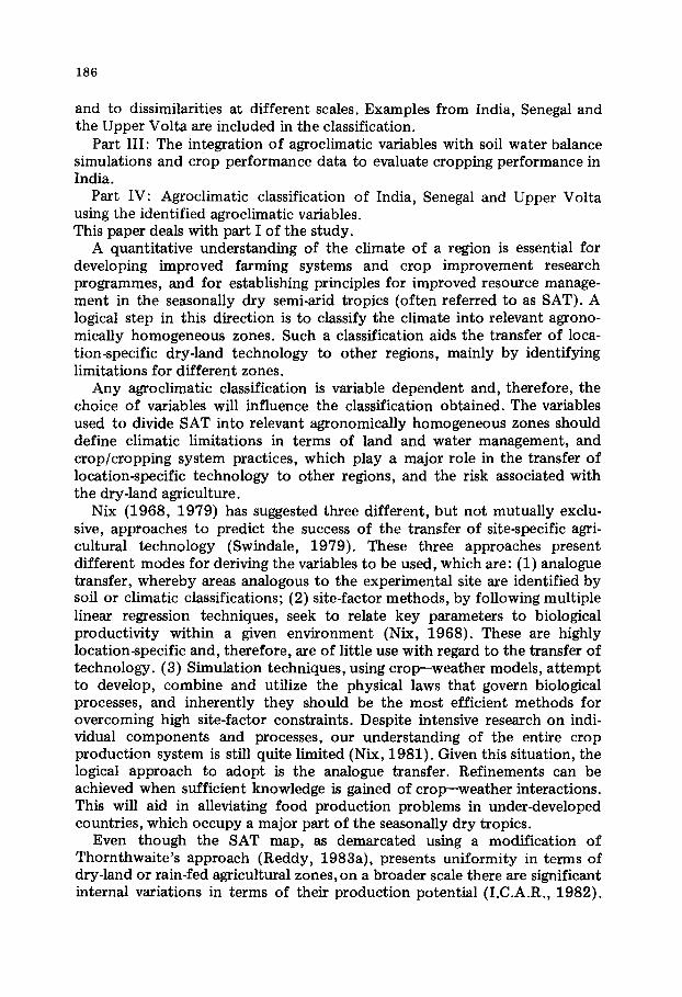
The National Bureau of Soil Survey and Land Use Planning has divided India into agroecological regions based on climatic and ecological conditions (Murthy and Pandy, 1978). The SAT is subdivided into four regions (Fig. la) and the third subdivision was further divided into two parts (Reddy and Virmani, 1980), namely (IIIa) undependable and (IIIb) dependable. Within all these subdivisions the rainfall amount varies significantly, from 600 to 1000 ram, and the length of the growing season varies between 90 and 180 days (Fig. la) . The growing season data has been based on the agro-ecological zones of FAO (Frere, personal communication, 1980) in which there are wide variations in terms of softs (Fig. lb ) and crops (I.C.A.R., 1982).

Farmers are not only interested in the available moist period but also the time it commences. In heavy clay soils (cf. vertisols), primary tillage and

188

seeding is difficult once the soil is wet. Thus, the time of commencement of sowing rains is also important for proper planning of seeding operations. The methods of Troll i1965) and Cocheme and Franquin {1967) rely on normal climatic data and, therefore, they do not take into account the variability of the weather from year to year on a seasonal basis. This is essential for identifying the proper crop/cropping pattern which is most productive with least risk. Even though the Hargreaves i1971, 1975) method is based on rain- fall at the 75% probability level, his estimates do not represent consecutive periods of the same year. This is important in understanding the probabilities of crop failure or near failure. Estimating the production potential of various regions, and the associated risk versus input levels, depends on knowledge of such probabilities.

Recently, several scientists (Nix, 1975; Russell and Moore, 1976; Russell, 1978; Austin and Nix, 1978; Gadgil and Joshi, 1981; Reddy and Virmani, 1982) have used numerical techniques for grouping locations according to agriculture. However, in the majority of these studies the data sets were the average of annual, monthly or weekly climatic data only. Some of these studies show anomalous groupings when compared with observed agricultural production patterns and with standard climatic classifications, like those of Koppen (1936), Thornthwaite (1948), Papadakis (1975), etc. Such anomalies are due more to the variables used than the classification procedure adopted.

Hence, variables estimated from average monthly, seasonal and annual rainfall based on long-term weather records have limited practical applica- bility in agricultural production studies. They can give a broad outline of productivity gradients but not of associated risks. While methods used to define the length and the beginning of the moist period were found to be of limited practical applicability using long-term average data, the basic con- cepts are very valuable aids for further development in this direction.

Therefore, in the present study, a modified method after Cocheme and Franquin i1967) and Hargreaves i1971, 1975) is suggested for estimating agroclimatic variables that are to be used to classify the climate of SAT into the relevant agronomically homogeneous zones. A comparison has been made between the results of the present approach and the three methods mentioned above.

METHODOLOGY

The meteorological data used and the sequence of steps followed to develop a method to derive classificatory agroclimatic variables for the relevant agronomically homogeneous zones of SAT are given below (Fig. 2).

i l ) Estimate RIPE for standard weeks 1--52 for 1--N years, where N represents the number of years for which the weekly rainfall (R) data are available iN should be more than 15 years and preferably more than 25 years to obtain meaningful statistical parameters). The details on the computation of potential evapotranspiration iPE) values for individual years were pre- sented by Reddy i1979).

189

1 . 6 ¸

~ 0 8 _ _ A B

E

~ g 0 4

Z u) u~

0 0 ~ I . . . . . . . . . . . . . . . . . . . . . . . . . , . . . .

3 °

, 0 - ./~ A w:,.eek0,.~

l o . [

I D = 5 weeks (A)

oo v i 4 26 30 32 34 36 3 46 48 50

Standard weeks

Fig. 2. Computat ion o f PS, S, G, W, and D (hypothet ical case for one year).

(2) For each week of the individual years, compute a 14-week moving average of RIPE centred around a particular week. In these computations, if R/BE >1 3.0 for any week then R/BE is set at 3.0. The 14-week moving average for weeks 20--21 is an average of the values for weeks 14--27, and the 14-week moving average for week 21--22 is an average of the values for weeks 15--28, etc. This procedure generates smoothed estimates of R/PE on a continuous basis for consideration of past and future moisture conditions. Short duration crops, like pearl millet and sorghum in SAT, require from 90--100 days from seeding to maturi ty. The 14-week (98<lay) moving average is chosen to reflect this duration. At least 7--8 weeks of opt imum moisture are required for a high yield.

(3) Determine the 'available effective rainy period G' as the consecutive period in the year which simultaneously fulfills the conditions:

(a) all weeks within period G have a 14-week moving average of R/PE ~>~ O.75;

(b) the week at the beginning of the period has a value of R/PE ~ 0.50 (a value of RIPE ~ 0.75 is chosen because this is in the opt imum range for plant growth).

This method is illustrated in Fig. 2 by taking a hypothetical case for one year. The upper part of the figure represents a 14-week moving average from A to B with RIPE more than 0.75. This excludes the period in which water is available to crops through soil water storage, which will be longer in the case of vertisols and shorter in the case of alfisols. The bo t tom curve in Fig. 2 represents the pattern of RIPE. The starting point, A, of the 14-week

190

moving average with R/PE >~ 0.75 lies between E and F, i.e., at E' (where R/PE >~ 0.50), and therefore G is represented by A--B (20.3 weeks). If the RIPE curve follows the dot ted line, to reach H from E, then RIPE would not be ~> 0.50 until I (after A), and in this case G is represented by J--B (17:4 weeks), which is less than A--B.

(4) The week before the beginning of the available effective rainy period is taken as the week of commencement of sowing rains (S).

This is week 20.5 for A and week 23.4 for J (Fig. 2). In this definition, the commencement of sowing rains of course differs from the onset or commencement of 'normal ' rain, as the former requires a threshold limit of rainfall to be satisfied. Generally, this is the amount needed to fill the top few centimetres of soil to the moisture content required to germinate seed in that environment. Here this is specified as RIPE >~ 0.50, in addition to a continuous moisture period later.

(5) Pre-sowing cultivation and seed-bed preparation (PS) are started when the 14-week moving average curve for RIPE crosses the 0.50 limit and when the particular week has RIPE >~ 0.25. In Fig. 2, PS is represented by week 19.

(6) Compute the number of weeks in the available effective rainy period for which R/PE >~ 1.5 and ~< 0.50, which are termed wet (W) and dry (D) spells, respectively.

In Fig. 2, if we consider G as A--B, then W = 7 weeks and D = 5 weeks; or if we consider G as J--B, then W = 7 and D = 3 weeks only. Hargreaves (1974) stated that during the rainy season, in months when MAI exceeded 1.34, in the semi-arid region of northeast Brazil, the moisture in the root zone was excessive and likely to hamper plant growth. The soils in this region are shallow, s tony and have a low organic matter and clay content . The SAT areas in India are primarily located on soils with a much higher water-holding capacity: vertisols and Indo--Gangetic alluvium (Fig. l b , Reddy and Virmani, 1980). It has been observed at the ICRISAT Centre that in the deep vertisols, short-term water-logging is quite common in the months of July, August and September. A significant detrimental effect of excessive water in the root zone is observed in September, when the soil profile is almost filled to capacity by the July and August rainfall. Based on this, Reddy and Virmani (1980) suggested that locations with 2 successive months with MAI of 0.66 or more pose a water-logging hazard. However, the above two limits can be approximated by RIPE of 2.0 and 1.0, respectively [Hargreaves (1975) observed that the dependable rainfall at 75% is linearly related to average monthly rainfall]. As a compromise between these two extremes, an intermediate value was chosen, i.e., R/PE of 1.5 or more, which is approximately equal to an MAI of 1.0.

Average yields in the U.S.A. are obtained in several mid-western states, where actual evapotranspiration rates average 72% of the potential rate. Crop failures are common when the actual evapotranspiration rates fall below 50% of the potential rate (Eagleman, 1976). This is also evident from the yield prediction equations of Jensen (1968), Hiler and Clark (1971)

191

and Minhas et al. (1974), as derived by Reddy (1983b), and from the results of Hiler et al. (1974).

Repeat steps 3a and b to 6 for N years. Let us say that for x years con- ditions 3a and b are not satisfied. Then one of two possible ways for calcu- lating the means and standard deviations (s.d.) for G, S, PS, W and D can be used.

(i) Assume for those years for which conditions 3a and b are not satisfied, that each of the 5 above-mentioned variables equal zero, then calculate the mean and s.d. for each of the 5 variables for N years. The mean and s.d. values for PS, S, W and D estimated using this assumption are misleading, with the means representing underestimates.

(ii) Consider years N -- x, for which conditions 3a and b are satisfied, com- pute the mean and s.d. values of PS, S, W and D for these years. The mean and s.d. estimated this way represent overestimates for G. However, possible wet and dry spells within the available effective rainy period, if they exist, are defined and this in fact is what an agronomist is interested in.

Thus, it appears that the first procedure is most suitable for estimating G, while the second procedure is best for the remaining 4 variables. Mean and s.d. for these 5 variables are denoted by G, S, PS, W and/9, and 0, 5, v, ~ and ~, respectively. There is some ambiguity jn the terms I~ and D in relation to G. That is, at lower values of G it is possible that IV + D ~ G, even though for individual years W + D is always ~ G. The error involved, however, is less than one week (overestimate) for both I~ and D which is considerably smaller than the s.d. (~,/3). However, there is no other way to overcome this problem. Hence, the procedure of least risk was followed, i.e., the first procedure for G and the second procedure for PS, S, W and D. The coef- ficient of variation (C) of the effective rainy period is computed as: C = (0 x 100)/G (C is used in association with G to compare its relative variation, as it represents the relative variation irrespective of the magnitude of G). In the case of PS, S, W and /9 the magnitude of variation is important com- pared to the relative variation (as will be appreciated in later sections), so only s.d. values are used.

(7) An arid situation (A) is defined as the percentage number of years for which G ~ 5 weeks. A 5-week period is considered to represent the minimal critical (reproductive) period with good moisture conditions for successful harvesting of a 98<lay crop._

The average effective rainy period (G) defines the available growing period (excluding the period that is available from the soil moisture reserve, which varies depending upon the soil type). This variable correlates with the type of cropping pattern, but is modified by the variation in the onset and cessa- tion times of sowing rain. This variability is defined here by the s.d. of the commencement of sowing rains (5) and the duration of the effective rainy period (C). When ~ and C are large the dependabil i ty of that cropping system is very low.

192

Therefore, careful planning is necessary before any system is adopted. The single most important factor is to determine the appropriate sowing time for opt imum utilization of available soil water. The mean week of commencement for sowing rains (S) is, therefore, an important factor in agricultural planning. The agricultural output at any location depends upon the level of inputs (e.g., fertilizers, weed management, cultural operations, etc.). However, it also depends upon the level of risk involved at a specific location. The aridity index (A) presents a measure of such risk in terms c f probable percentage crop failures.

Vertisols and associated softs in India cover ~ 73 x 106 ha (Fig. lb) , which constitute ~ 22% of the total area of the country. These soils alsc occur extensively in northern Australia, Sudan, Ethiopia and in smaller areas of sub-Saharan Africa, particularly Chad, Tanzania. Smaller areas occur in Mexico, Central America, Venezuala, Bolivia and Paraguay (ICRISAT, 1981). Water-logging is a major problem in these soils, which are charac- terized by low infiltration rates, but is not usually an important problem in most other soils. Primary tillage and seeding in deep, cracked clay soils (vertisols) is difficult once the rains have commenced. In general, therefore, they are left fallow during the rainy season and are cropped only in the post-rainy season (except in Sudan and east Africa). This practice does not facilitate opt imum utilization of natural resources in terms of potential cropping and also increases runoff and soil erosion. The timing of tilling is the key to successful cropping, otherwise weeds become unmanageable and yields are substantially reduced. Thus, dry,seeding techniques, applied before the rains, may overcome these difficulties to a certain extent. (Dry- seeding anticipates the commencement of rains by a few days and with the first rains the seed germinates. Dryseeding is feasible where the onset t ime of rains is reliable and was found successful at ICRISAT Centre.) This technique is in fact practiced by farmers in some parts of India, particularly in the Akola region. In regions where water-logging is a major problem proper management of soil and water is critical. Dry-seeding is only feasible where rains regularly commence at the same time each year. The s.d. of commencement of sowing rain (6) can provide a measure of the likely suitability of dry,seeding in different regions. Similarly, the mean occurrence of wet spells (W) can be used to assess the water_-logging hazard at a specific location. Wet spells, along with the dry spells (D), and their respective s.d. (a, ~) can be used to assess the suitability of a region for dry-land agriculture. These parameters can indicate the probable duration and variability of periods suitable for agricultural operations within the rainy season; they can be used to assess the potential for runoff recycling to increase produc- tion, particularly in soils with low water-holding capacity; and they can be used to estimate the duration of dry spells in relation to the growth patterns of specified crops.

193

DISCUSSION

Tile method outlined above (hereafter referred to as the R-method) is an extension of the concepts of Cocheme and Franquin (1967, CF-method) and Hargreaves (1974 and 1975, H-method). The CF-method considers the moist period based on a normal monthly data set, while the R-method estimates the moist period on the basis of weekly data for individual years using a moving average technique. The H-method is based on rainfall prob- abilities for individual and independent months, while the R-method takes into account actual t ime sequences, year by year, over the entire moist period. The R-method, therefore, incorporates all the important and useful features of the CF- and H-methods, and it also gives some useful additional information. Table I presents these parameters for a few selected Indian stations. For example, in the case of Bangalore, the s.d. of G (0) is very high, but at Agra is very small. This correlates with the observed instability of food production at Bangalore compared with Agra. The variability over time of the commencement of sowing rains is also wide (5 is 4.7 weeks at Bangalore and 1 week at Agra). Thus, while proper planning of the sowing t ime is very critical at Bangalore it is much less so at Agra. In many years there is a possibility of crop failure at Bangalore (A = 32% of the years) compared to Agra (A = 8% of the years). At Bangalore, the instability of crop product ion can be reduced by proper management of water, through recycling of runoff during d_r2y spells, as there is a possibility of obtaining useful runoff in many years [W + a = 3.9 + 3.1 weeks, I.C.A.R., 1982).

On the red softs (alfisols) of Bangalore, only the late kharif (or rainy season) crop is successful while on the alluvial soils of Agra double crops are successful (Singh et al., 1974; Spratt and Choudhury, 1978; I.C.A.R., 1982). Crop product ion is stable at Agra compared to Bangalore, where proper planning of the sowing time (August or September) is very critical (irrespective of soil type). By comparison, the H-method suggests that crop production is stable at Bangalore, with one or two crops with MAI 0.34 for 6 months, while at Agra it is unstable and risky, with MAI ~ 0.34 for 2 months only (Table II). At Jodhpur , cropping intensity varies from 30 to 100%, while at Anantapur it ranges from 100 to 125% and in years of early rains double cropping could be practiced (as referred to above). The contrary is evident from Troll's (1965) approach (as modified by Reddy, 1977) (Table II), with 0 and 1 humid months at Anantapur and Jodhpur , respectively.

According to the CF-method, the difference between Allahabad and Indore is negligible (Table II), and this is also evident from G (Table I), but the R-method suggests, in addition, that the percentage of crop failure years due to drought are zero at these places and the variation in the com- mencement of sowing rains is small (5 = 1.3 to 1.4 weeks). Therefore, dry-seeding is feasible in the vertisol regions of Indore, whereby two crops could be grown (Spratt and Choudhury, 1978). Traditionally, however, only one crop is grown in the post-rainy season, on land fallowed during the rainy

TA

BL

E I

Cli

mat

ic c

lass

ific

atio

n re

sult

s ba

sed

on

th

e p

rese

nt

(R-m

eth

od

) ap

pro

ach

~ 6

0 S

ampl

e n

o.

Sta

tio

n

(wee

k n

o.)

(w

eeks

) (w

eeks

) (w

eeks

) (w

eeks

) (w

eeks

) (w

eeks

) (w

eeks

) A

(%

Y)

1 A

llah

abad

25

.1

1.4

16.5

3.

5 2

Ind

ore

24

.7

1.3

16

.4

3.1

3 B

anga

lore

27

.4

4.7

11

.8

8.4

4 A

gra

26.3

1.

0 13

.3

3.6

5 A

nan

tap

ur

35

.5

4.8

5.2

5.4

6 Jo

dh

pu

r 29

.0

2.1

2.6

4.4

7 R

aneh

i 23

.9

2.9

16

.4

3.8

7.0

7.0

3.9

5.9

2.7

2.9

7.5

2.1

2.2

3.1

2.0

1.7

1.1

3.4

5.3

6.0

5.2

5.1

3.7

3.3

3.7

2.0

2.1

3.9

1.9

2.5

2.1

1.8

0 0 32 8

52

73 0

TABLE II

Climatic classification results based on various approaches

195

R' PE' T H CF (days) Sample no. S ta t ion Soil t y p e d (mm) (mm)

h m md

1 Allahabad Alluvial 1027 1537 3 a 3 a 95 120 175 2 Indore Black 1053 1813 3 a 3 a 100 120 155 3 Bangalore Red 924 1501 4 a 6 b 115 205 235 4 Agra Alluvial 765 1467 3 a 2 c 75 100 120 5 Anan tapur Red 562 1857 0 c 1 c 0 90 200 6 J o d h p u r Sierozem 380 1843 1 c 0 c 0 60 80 7 Ranchi Red 1463 1304 4 a 4 a 130 163 240

asemi-arid; b sub-humid or wet dry; C arid; dalluvial = entisols , black = vertisols, red =: alfisols, s ie rozem = aridisols. R ' = mean annual p rec ip i ta t ion ; PE'= mean annual po ten t i a l evapot ransp i ra t ion ; R" =: mean m o n t h l y prec ip i ta t ion (mm) ; R ' ---- mean m o n t h l y prec ip i ta t ion $ s tored soil water (mm) ; P E = m e a n m o n t h l y po ten t ia l evapot ransp i ra t ion (mm). T = Troll 's (1965) approach : n u m b e r of humid (R":>PE) m o n t h s (as modi f i ed by Reddy , 1977). H =: Hargreave 's (1971) approach : n u m b e r of m o n t h s wi th MAI ~ 0.34 ; CF ---- Cocheme and F r a n q u i n ' s (1967) a p p r o a c h ; h ---- humid (R ~ PE ) per iod (days) ; m = mois t (R ~ 0.5 PE)., per iod (days); m d = mois t - -d ry (R ~ 0.25 PE) per iod (days).

season, using stored soil water. Field working days are also significantly more at Indore compared to Allahabad, W = 7.0 and D = 6.0 weeks at Indore, and

= 7.0 and D = 5.3 weeks at Allahabad. This facilitates the use of dry-land agriculture to grow crops like sorghum at Indore and paddy-rice at Allahabad (Fig. 3). For example, also see Ranchi (Ranchi comes under the sub-humid or wet_---dry zone and Indore comes under semi-arid zone),_where the dry spells (D = 3.7 weeks) are far fewer compared to wet spells (W = 7.5 weeks), where dry-land agriculture is less productive (particularly in the vertisols region). Upland rice is the major crop in the vertisols region of Ranchi in the rainy season (Mohsin and Sinha, 1979; Fig. 3).

In India, a large part of regions with deep vertisols (Fig. l b ) are kept fallow during the rainy season and are cropped only in the post-rainy season (Table III). It appears from this table that the reasons for this practice are due to (1 )h igh 5, undependable timing of initial rains, or (2) high W along with low D, high water-logging problem with less available days for field work. In the former case, proper identification of sowing times (S) is critical for crop production, and in the latter situation this can be reduced by dry-seeding where the timing of initial rains is reliable (5 is small). Dry- seeding is carried out a week before the onset of rains (based on local fore- casts), generally before S and after S - 5/2. However, in the former case, sowing can be carried out after S and before S + 5/2 (based on local fore- casts) [see experimental evidence for a few Indian locations, I.C.A.R. (1982)] . For example, at Bellary a post-rainy season (or rabi) crop is more assured than a rainy season (or kharif) crop. The traditional sowing times at

196

I 58 +

~o

8+

INDIA

Crop region

~ R i c e

Pearl mil let

Sorghum

- - SAT boundary

.Source Easter and Abel 1973 ~ 0 500 1000 km

76o 84" 92°E

Fig. 3. Rice, pearl millet and sorghum cropping regions.

BeUary are not the best (Spratt and Choudhury, 1978), but yields could be increased by advancing the date of sowing to September (Singh et al., 1974). The mean week of commencement of sowing rains (S), week 35, agrees very well with this finding. Similarly, at Hyderabad, it was found that dry-seeding was successful with ~ = 2.9 weeks, while at Sholapur, with ~ = 4.0 weeks, it was a failure (Binswanger et al., 1980).

CONCLUSIONS

Based on actual time sequences of weekly rainfall and potential evapo- transpiration data over periods of more than 15 years duration, a method for deriving agroclimatic variables to assess the agricultural product ion potential of a region has been developed. This method is used to define the

TABLE III

Climatic variables and percentage area under kharif (rainy season) fallow for selected locations in the deep vertisol regions of India

197

Location Climatic variables

l~ G A Area under kharif (weeks) (%) fallow (%)

Undependable rainfall zone (with high 6 -zone of erratic initial rains) Ahmednagar 4.9 3.4 9.2 33 57.3 Sholapur 4.0 3.6 11.3 24 74.3 Poona 4.1 3.6 12.1 15 44.0 Aurangabad 3.0 4.5 13.2 12 40.3 Hyderabad 2.3 4.2 12.9 13 25.0

Dependable rainfall zone (with high l~-water-logging zone) Jabalpur 1.5 9.8 18.5 00 50.0 Indore 1.3 7.0 16.4 00 44.2

mean week of commencement of sowing rains (S) and its variability (5); the mean available effective rainy period (9) and its variability (0); the mean number of wet and dry weeks within the available effective rainy period (I~ and /)) and their variabilities (~, ~); and the percentage crop failure years or level of risk associated with dry-land agriculture (A). This procedure has been developed with special reference to SAT.

Determination of S , P S and 5, u help to assess the feasibility of dry- seeding, the proper period for so_wing, land preparation, etc. Dry-seeding is less favourable where 5 is high. G and C play a significant role in planning the crop/cropping pattern to be followed at a particular location and the risk associated with such a system. A explains the risk associated in the crop production and, therefore, the input levels. Measurement of W, D and a, help to determine the feasibility of runoff collection and its recycling during drought periods to reduce the risk. They also aid in assessing the water- logging situation, the intensity of soil erosion and in estimating the days available for field work, and thereby developing the measures of soil manage- ment to overcome these problems.

ACKNOWLEDGEMENTS

This s tudy was carried out during a stay at the Australian National Univer- sity, Canberra. The author expresses his gratitude to the Australian National University for financial support and Drs. H.A. Nix and N.S. McDonald for their valuable discussions and comments on the draft . The author is also thankful to Mr. K.A. Cowen for cartographic assistance.

198

SYMBOLS

R PE MAI DP

SAT

0 C

o~

S

PS p

Rainfall (mm) Potential evapotranspiration (mm) Moisture availability index (DP/PE) Dependable precipitation (estimated using long-term data by fitting to incomplete 7 distribution) at 75% probability level (mm)

. . . . ~ O Semi-arid tropms (with mean annual temperature - / 1 8 C and annual moisture index, Im ( R - PE/PE × 100) varying between - -25 and --75% (Reddy, 1983a) The mean available effective rainy period (weeks) Standard deviation of G (weeks) Coefficient of variation of G(O x 100/G) (%) The mean wet spell within G period (weeks) Standard deviation of W (weeks) The mean dry spell within G period (weeks) Standard deviation of D (weeks) The mean week of commencement of sowing rains (week no.) Standard deviation of S (weeks) The mean week of pre-sowing cultivation (week no.) Standard deviation of PS (weeks)

REFERENCES

Austin, M.P. and Nix, H.A., 1978. Regional classification of climate and its relation to Australian rangeland. In: Studies of the Australian Arid Zone, III, Water in Rangelands. CSIRO, Melbourne, pp. 9--17.

Binswanger, H.P., Virmani, S.M. and Kampen, J., 1980. Farming system components for selected areas in India: evidence from ICRISAT. Res. Bull. 7, ICRISAT, Patancheru, India.

Cocheme, J. and Franquin, P., 1967. A study of the agroclimatology of the semi-arid area south of the Sahara in West Africa. FAO/UNESCO/WMO Interagency Project on Agroclimatology, Tech. Rep., Rome, pp. 117--129.

Eagleman, J.R., 1976. The Visualization of Climate. Lexington Books, D.C. Heat, Toronto, 256 pp.

Gadgil, S. and Joshi, N.V., 1981. Use of principal component analysis in rational classi- fication of climates. In: Proc. on Climate Classification: A Consultants' Meeting. ICRISAT, Patancheru, India, pp. 17--26.

Hargreaves, G.H,, 1971. Precipitation dependability and potential for agricultural produc- tion in Northeast Brazil. Rep. 74-D159, EMBRAPA and Utah State University, 123 PP.

Hargreaves, G.H., 1974. Climatic zoning for agricultural production in Northeast Brazil. Utah State Univ., U.S.A.I.D., Contract AID/CSD 2167, 16 pp.

Hargreaves, G.H., 1975. Water requirements manual for irrigated crops and rainfed agriculture. EMBRAPA and Utah State University, Rep. 75-D158, 40 pp.

Hiler, E.A. and Clark, R.N., 1971. Stress day index to characterize effects of water stress on crop yields. Trans. ASAE, 14: 757--761.

Hiler, E.A., Howell, T.A., Lewis, R.B. and Boos, R.P., 1974. Irrigation timing by the stress day index method. Trans. ASAE, 17: 393--398.

199

I.C.A.R. (Indian Council of Agricultural Research), 1982. A decade of dry-land agricul- tural research in India 1971--80. All India Co-ordinated Research Project for Dry-land Agriculture (ICRPDA), Saidabad, Hyderabad, India.

ICRISAT, (International Crops Research Inst i tute for the Semi-arid Tropics), 1981. Improving the management of Indian deep black soils. Indian Ministry of Agric./ I .C.A.R./ICRISAT. ICRISAT Patancheru, India, 106 pp.

Jensen, M.E., 1968. Water consumption by agricultural plants. In: T.T. Kozlorvoski (Editor), Water Deficits and Plant Growth, Vol. II. Academic Press, New York, pp. 1-- 22.

Koppen, W., 1936. Das Geographische System der Klimate. In: W. Koppen and R. Giner (Editors), Handbuche der Klimatologie, Vol. I, Part C. Gerbrender Borntrager, Berl in

Minhas, B.S., Parikh, K.S. and Srinivasan, T.N., 1974. Towards the structure of a produc- tion function for wheat yields with dated inputs of irrigated water. Water Resour. Res., 10: 383--393.

Mohsin, M.A. and Sinha, N.P., 1979. Rain-fed agricultural technology for Bihar. Presented at Kharif Workshop of the Dept. Agric., Patna, India, 16 pp.

Murthy, R.S. and Pandey, S., 1978. Delineation of agro-ecological regions of India. In: Proc. Commission V, l l t h Congress of the Int. Soc. Soil Sci., Edmonton, Canada.

Nix, H.A., 1968. The assessment of biological productivity. In: G.A. Stewart (Editor), Land Evaluation. MacMillan, Melbourne, pp. 77--87.

Nix, H.A., 1975. The Australian climate and its effects on grain yield and quality. In: A. Lazenby and E.M. Matheson (Editors), Australian Field Crops, I: Wheat and other Temperate Cereals. Angus and Robertson, Sydney, pp. 183--226.

Nix, H.A., 1979. Agroclimatic analogues in transfer of technology. In: Proc. Intern. Symp. on Development and Transfer of Technology for Rain-fed Agriculture and the SAT Farmer. ICRISAT, Patancheru, India, pp. 83--88.

Nix, H.A., 1981. Simplified simulation models based on specific minimum data sets: the CROPEVAL concept. In: A. Berg (Editor), Applicat ion of Remote Sensing for Agri- cultural Production Forecasting. Balkema, Rot terdam, pp. 151--169.

Papadakis, J., 1975. Climates of the World and their Agricultural Potentialities. Cordoba, Spain.

Reddy, S.J., 1977. A review - -agroc l imat ic classification. ICRISAT, Patancheru, India, 41 pp.

Reddy, S.J., 1979. User's manual for water balance models. ICRISAT, Patancheru, India, 28 pp.

Reddy, S.J., 1983a. Climatic classifications: The semi-arid tropics and its e n v i r o n m e n t - a review. Pesq. Agropecu. Bras., 18 : 823--847.

Reddy, S.J., 1983b. Irrigation scheduling using ICSWAB model. 2 Pesq. Agropecu. Bras., 18: in press.

Reddy, S.J. and Virmani, S.M., 1980. Pigeonpea and its climatic environment. In: Proc. a review. Pesq. Agrop. Bras. (Brazil), 18:

Reddy, S.J., and Virmani, S.M., 1980. Pigeonpea and its climatic environment. In: Proc. Intern. Workshop on Pigeonpea, ICRISAT/ICAR. ICRISAT, Patancheru, India, pp. 259--270.

Reddy, S.J. and Virmani, S.M., 1982. Grouping of climates of India and West Africa: using principal component analysis. ICRISAT FSRP, Agroclimatology Annu. Rep. 1980--1981 (Progress Rep. 5). ICRISAT, Patancheru, India, pp. 21--25.

Russell, J.S. and Moore, A.W., 1976. Classification of climate by pat tern analysis with Australian and southern African data as an example. Agric. Meteorol., 16: 45--70.

Russell, J.S., 1978. Classification of climate and potential usefulness of pattern-analysis techniques in agroclimatology research. In: Proc. Agroclimatological Research Needs of the Semi-arid Tropics. ICRISAT, Patancheru, India, pp. 47--58.

Singh, R.P., Singh, A. and Ramakrishna, Y.S., 1974. Cropping patterns for dry-land of India -- an agroclimatology approach. Ann. Arid Zone, 13: 145--164.

200

Spratt, D. and Choudhury, S.L., 1978. Improved cropping systems for rain-fed agriculture in India. Field Crops Res., 1 : 103--126.

Swindale, L.D., 1979. Problems and concepts of agrotechnology transfer within the tropics. In: Intern. Syrup. on Development and Transfer of Technology for Rain-fed Agriculture and the SAT Farmer. ICRISAT, Patancheru, India, pp. 73--82.

Thornthwaite, C.W., 1948. An approach towards a rational classification of climate. Geogr. Rev., 38: 55--94.

Troll, C., 1965. Seasonal climates of the Earth. In: E. Rodenwaldt and H. Jusatz (Editors), World Maps of Climatology. Springer-Verlag, Berlin, 28 pp.