agriculture in the tongue river basin: output, water quality, and
TRANSCRIPT
i
Agricultural Marketing Policy Center
Linfield Hall
P.O. Box 172920
Montana State University
Bozeman, MT 59717-2920
Tel: (406) 994-3511
Fax: (406) 994-4838
Email: [email protected]
Web site: www.ampc.montana.edu
This publication was developed with financial
support from the Risk Management Agency
USDA and the University of Wyoming.
Agriculture in the
Tongue River Basin: Output, Water Quality,
and Implications
Timothy Fitzgerald
Assistant Professor
Department of Agricultural Economics and Economics
Montana State University
Grant Zimmerman
Research Assistant
Department of Agricultural Economics and Economics
Montana State University
Agricultural Marketing Policy Paper No. 39 May 2013
ii
ACKNOWLEDGEMENTS
We would like to thank the contribution of many individuals who assisted us in understanding the
agricultural economy and complex water quality system of southeastern Montana. We
particularly thank Steve Anderson, James Bauder, Alexis Bonogofsky, Chuck Dalby, Nick
Golder, John Hamilton, Art Hayes, Les Hirsch, Jim Johnson, Wally McRae, Robert Mitchell,
Roger Muggli, Brad Sauer, Adam Sigler, Vince Smith, and Myles Watts. We are especially
indebted to William Moore for his help with a large part of the geospatial analysis. An earlier
version of this report was presented at the Montana Section of the American Water Resources
Association annual meeting—we would like to thank participants in those meetings for useful
comments. Thanking these individuals in no way implicates any of them in any remaining
errors, for which we accept full responsibility.
iii
TABLE OF CONTENTS
LIST OF TABLES ........................................................................................................................ IV
LIST OF FIGURES ........................................................................................................................ V
LIST OF ABBREVIATIONS ....................................................................................................... VI
EXECUTIVE SUMMARY ......................................................................................................... VII
INTRODUCTION .......................................................................................................................... 1
BACKGROUND ............................................................................................................................ 2
Previous Studies ........................................................................................................................ 5
AGRICULTURAL PRODUCTION ............................................................................................... 6
Crop Results ............................................................................................................................ 11
Alfalfa ............................................................................................................................... 11
Barley ................................................................................................................................ 12
Corn................................................................................................................................... 13
Cattle Results .......................................................................................................................... 15
Total Value.............................................................................................................................. 18
WATER QUALITY AND ITS EFFECTS ................................................................................... 21
Data ......................................................................................................................................... 23
Identifying Changes ................................................................................................................ 24
Weather Data .......................................................................................................................... 25
Does Water Quality Variation Affect Agricultural Production? ............................................ 26
DISTRIBUTIONAL IMPLICATIONS ........................................................................................ 27
Soils......................................................................................................................................... 27
Irrigation and Soil Type .................................................................................................... 27
Tax Implications ..................................................................................................................... 28
Potential Impacts ............................................................................................................... 30
GENERAL DISCUSSION & CONCLUSIONS .......................................................................... 33
REFERENCES ............................................................................................................................. 34
APPENDIX ................................................................................................................................... 36
DATA SOURCES AND METHODOLOGY............................................................................... 36
Additional Tables .................................................................................................................... 40
iv
LIST OF TABLES
1. All Hay vs. Irrigated Hay, Acreage and Yield, Southeast Montana Agricultural District, 2000-
2008, Average Values. .................................................................................................................... 3
2: Coalbed Methane Wells, September 2012. ................................................................................ 5
3: Montana Crop and Irrigation Choices: 2008. ............................................................................ 7
4: Montana Price Series for Agricultural Commodities. ............................................................... 9
5: 2011 Primary Cover. ................................................................................................................ 10
6: Salinity Tolerance of Crops. .................................................................................................... 22
7: Irrigated Soil Types ................................................................................................................. 28
8: Acreage by County and Tax Assessment Category. ................................................................ 29
9: Mean Dollars Assessed Value Per Acre of Land Classifications. ........................................... 29
10: Agricultural Land Tax Receipts, 2012. .................................................................................. 30
11: Tax Assessment Implications of Loss of Irrigation. .............................................................. 31
12: Tax Revenue Implications of Loss of Irrigation. ................................................................... 31
13: Capitalization of Loss of Tax Revenue.................................................................................. 32
v
LIST OF FIGURES
1: Map of Tongue River Basin....................................................................................................... 3
2: Map of T&Y Irrigation District ................................................................................................. 4
3: Acres Irrigated with Tongue River Water ................................................................................ 8
4: Alfalfa Acres ............................................................................................................................ 11
5: Alfalfa Production.................................................................................................................... 12
6: Barley Production .................................................................................................................... 13
7: Corn Acres ............................................................................................................................... 14
8: Grain Corn Production ............................................................................................................. 15
9: Estimated Cattle Inventory ...................................................................................................... 16
10: Average Weight per Marketed Head of Cattle, Montana 1980-2010 .................................. 17
11: Estimated Cattle Gross Revenue............................................................................................ 18
12: Aggregate Gross Value .......................................................................................................... 19
13: Comparison of Gross Revenue Measures .............................................................................. 20
14: Gross Value Forecast ............................................................................................................. 21
15: USGS Water Monitoring Sites .............................................................................................. 23
16: Tongue River Flow at State Line ........................................................................................... 24
17: Seasonal Variation in SAR .................................................................................................... 25
18: Palmer Drought Severity Index ............................................................................................. 26

vi
LIST OF ABBREVIATIONS
AMPP: Agronomic Monitoring and Protection Program
CBM: Coalbed methane
CDL: Cropland Data Layer
DOR: Department of Revenue
FRIS: Farm and Ranch Irrigation Survey
NASS: National Agricultural Statistics Service
PDSI: Palmer Drought Severity Index
SAR: Sodium Absorption Ratio
SC: Specific Conductance
USDA: United States Department of Agriculture
USGS: United States Geologic Survey
TRB: Tongue River Basin
TRIP: Tongue River Information Project
T&Y: Tongue & Yellowstone
vii
EXECUTIVE SUMMARY
This study considers the value of an important natural resource in Montana—the Tongue River
basin and specifically the water it supplies for irrigated agriculture in the southeastern part of the
state. The study identifies the agricultural value that could be at risk due to water quality
changes, describes how the water resource is measured, and explores the possible impacts of
changes in water availability. Along the length of the river, 25,000 acres are irrigated with water
drawn from the main stem (we do not count acreage that is subirrigated or watered directly from
tributaries).
These are the first panel estimates of agricultural production for section of the Tongue River
Basin located in Montana. Existing annual county estimates compiled by the National
Agricultural Statistics Service (NASS) were allocated using spatial weighting algorithms. Our
technique is similar to those used to obtain other estimates of watershed-level production but, we
argue, an improvement over those approaches. Satellite data on land cover were used to
construct spatial weights. The estimated series were used to generate physical production series
for the basin in the years 1980-2010. Individual data series were estimated for the primary
agricultural products in the basin: alfalfa, barley, corn, and cattle. In recent years the gross
revenue obtained from sales of these primary crops has exceeded $22 million each year and in
recent years has been increasing. Projecting the trend forward over the next thirty years leads to
a forecast of $1.3 billion in nominal gross revenue over that time period.
Extensive data on water quantity and water quality at various locations over time along the
Tongue River are available from the United States Geological Survey. In addition to flow
measurements, these data include measures of irrigation water quality. Irrigators are concerned
about water salinity, because using saline water can damage soil under certain conditions,
leading to long-term productivity declines. This study focuses on two of the most pertinent
measures of salinity: specific conductance and the sodium absorption ratio. These data are
presented with an emphasis on identifying the background variation in flows and quality in the
river. Data on water quality are available only for relatively short periods compared to flow and
agricultural data, a problem compounded by the fact that monitoring sites have moved over time.
Thus, water quality variation in the river does not appear to be conclusively and causally
associated with agricultural production and gross revenue in the watershed.
Additional interesting inferences about the agricultural economy of the Tongue River basin are
obtained from an analysis of tax assessment data for agricultural land in the basin. The total
assessed value of agricultural land in the basin is over $165 million; the land is combined with
water, livestock, equipment, and other improvements to generate the agricultural product. A
prospective loss of all irrigated acreage along the Tongue is estimated to reduce assessed value
by over $6 million, and capitalized property tax collections on agricultural land by $1 million.
1
INTRODUCTION
Natural resources have long been important to economic activity in Montana. From wildlife
populations to mineral deposits, different residents have recognized the natural potential of the
state and worked to create wealth from different resources. Agriculture has been and remains an
important means of creating economic value from natural resources—gross revenues from
agriculture are larger than any other sector in Montana, though it ranks lower in terms of
contribution to gross domestic product.1 This study considers the value of a specific natural
resource in Montana—water quality in the Tongue River in the southeastern part of the state.
The study has three main sections: the first documents the agricultural production of the region;
the second evaluates the importance of water quality to that production; and the third considers
the distributional implications including contribution to public finances.
Although the region in which the Tongue River Basin (TRB) is located has the longest growing
season of any portion of the state, the aridity of the climate makes agricultural production in the
basin heavily dependent on irrigation water from the Tongue River. While the available quantity
of water is clearly an important aspect of natural resource use, the quality of that water is also
important to continued agricultural productivity. Because water quantity and quality are related,
both dimensions of the resource have to be considered in any analysis of agricultural production
and its value to the regional economy.
This study makes three contributions towards a better understanding of the importance of
irrigation in the Tongue River Basin and the role natural resources play in agriculture more
broadly. The first is to provide a long-run description and summary of agricultural activity in the
basin. This unique long-term estimate of annual agricultural gross revenue captures the pertinent
scale at which natural resources and agriculture interact. Second, the existing record of water
quality measurements is examined. While causal effects on aggregate agricultural output are not
identified, the nature of the available data itself highlights the value of consistent data collection.
Third, agricultural productivity is connected to distributional measures, including the taxable
value of the land and potential revenue collections.
These results are likely to interest many groups. Local government officials, producers, and
other interested community members continue to seek answers to questions on this subject that
have remained open for years. Local producers will be interested in the original valuations of the
TRB as well as the more specific distributional data. Water quality regulators might be
interested in the stated model to measure the opportunity cost of water quality changes as well as
part of a broader discussion of appropriate water quality protections. Third, policymakers and
others considering further energy infrastructure investments in the region might consider the
impacts that water quality changes have on the existing agricultural economy. The estimates
presented here are based on the production value of an ecosystem service, which is only one way
to address likely impacts on a watershed level.2
Amid broader policy debates about natural resource use, the agricultural sector is largely taken
for granted. One objective of this study is to consider more deeply the opportunity costs
imposed on agriculture by alternative use of natural resources. Other studies estimate minimal, if
1 Annual gross revenue from agriculture has exceeded $3.5 billion in recent years, with a somewhat higher
contribution from crops than livestock (NASS). Among natural resource industries (agriculture, mining, oil & gas,
tourism, and timber), this is the largest contribution. However, energy (oil & gas plus coal) makes a larger
contribution to value added. 2 For an example of a study in the same region that focuses almost exclusively on employment effects, see Barkey
and Polzin (2012).
2
any, impacts on agriculture from development of other natural resources. However, because
agriculture relies on interconnected resources, impacts of changes in the quality of natural
resources could be relatively large under some scenarios.
BACKGROUND
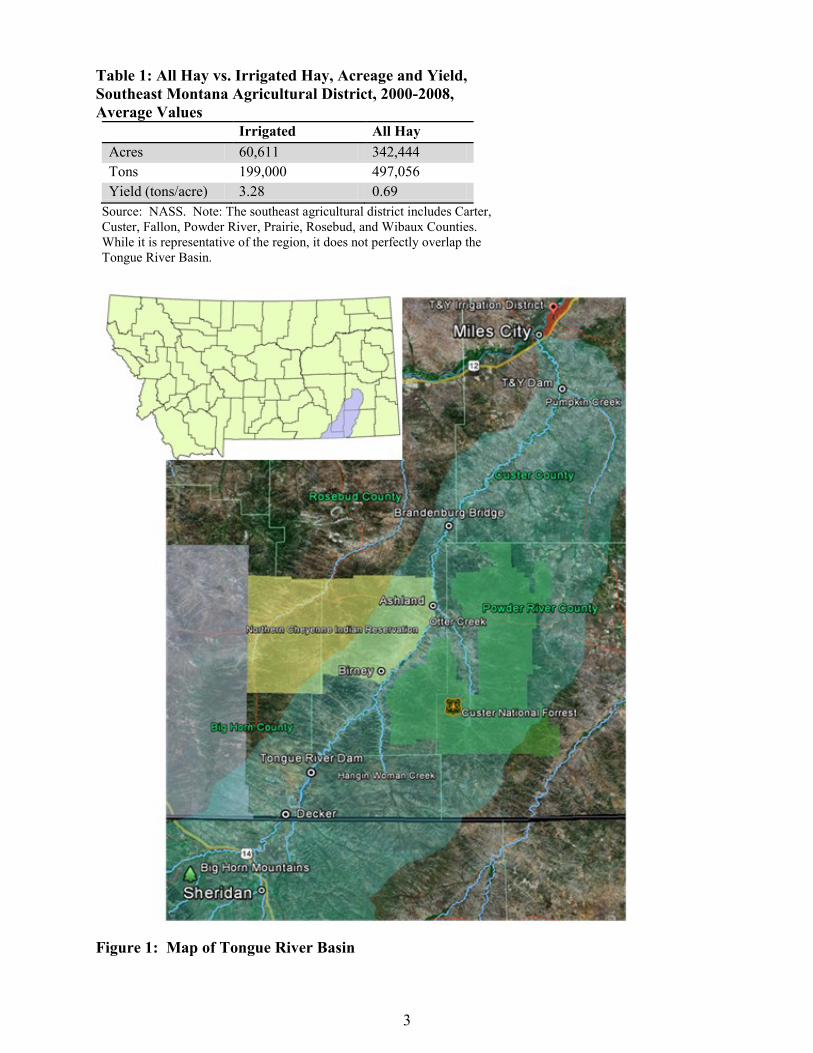
From its headwaters in the Big Horn Mountains in Wyoming, the Tongue flows approximately
250 miles along a northeasterly course to its confluence with the Yellowstone River at Miles
City, Montana. The watershed drains over 5,400 square miles; thirty percent of the total
watershed area is in Wyoming and 70 percent (nearly 2.5 million acres) in Montana. Just after
crossing the Montana state line the river flows into the Tongue River Reservoir. The reservoir is
administered by the Tongue River Water Users' Association; the reservoir stores water for 35
irrigators along the river. When full to capacity, the reservoir stores 150,000 acre-feet of water.
Below the reservoir are confluences with important tributaries: Hanging Woman Creek at
Birney, Otter Creek at Ashland, and Pumpkin Creek about 12 miles before the river reaches
Miles City. Near the Pumpkin Creek confluence is the diversion point for the Tongue &
Yellowstone (T&Y) canal, where a significant share of water is diverted for irrigation. The T&Y
canal provides water to 9,000 of the 25,000 acres irrigated by the Tongue, including about 4,800
acres along the Yellowstone River northeast of Miles City, outside the hydrologic boundary of
the basin. However, because the area uses a significant share of water from the river, it is
included in the analysis. About 7,800 of the 25,000 acres are irrigated by center pivot sprinkler.
Over its course, the Tongue and its tributaries pass through four Montana counties: Big Horn,
Rosebud, Powder River, and finally Custer. The river itself does not flow through Powder River
County, but tributaries that drain a large area do. The river serves as the eastern border of the
Northern Cheyenne Reservation as well as the watershed for a significant portion of the Custer
National Forest. Figure 1 is a map of the Tongue River Basin area.
Agriculture dominates the local economy, although nearby energy developments make
significant contributions to county-level economic aggregates. Miles City is a regional
commerce hub and the largest population center in eastern Montana. The agricultural economy
is based largely on range cattle production with supporting farming operations. Seasonal grazing
is important for both domestic livestock and wildlife. Ranching with seasonal range use is
facilitated by the availability of irrigation water that helps increase forage yields in the river
bottom, producing sufficient winter feed for livestock that utilize the uplands during the growing
season. In addition to range cattle operations, there are also several small-scale agricultural
operations that grow a variety of crops catering to local consumer markets.
As table 1 indicates, yield gains from irrigation are substantial in the region, though considerable
harvest occurs on dryland acres as well. However, 40 percent of total production comes from
irrigated land, which amounts to about one-sixth of total acreage.
3
Table 1: All Hay vs. Irrigated Hay, Acreage and Yield,
Southeast Montana Agricultural District, 2000-2008,
Average Values
Irrigated All Hay
Acres 60,611 342,444
Tons 199,000 497,056
Yield (tons/acre) 3.28 0.69
Source: NASS. Note: The southeast agricultural district includes Carter,
Custer, Fallon, Powder River, Prairie, Rosebud, and Wibaux Counties.
While it is representative of the region, it does not perfectly overlap the
Tongue River Basin.
Figure 1: Map of Tongue River Basin
4
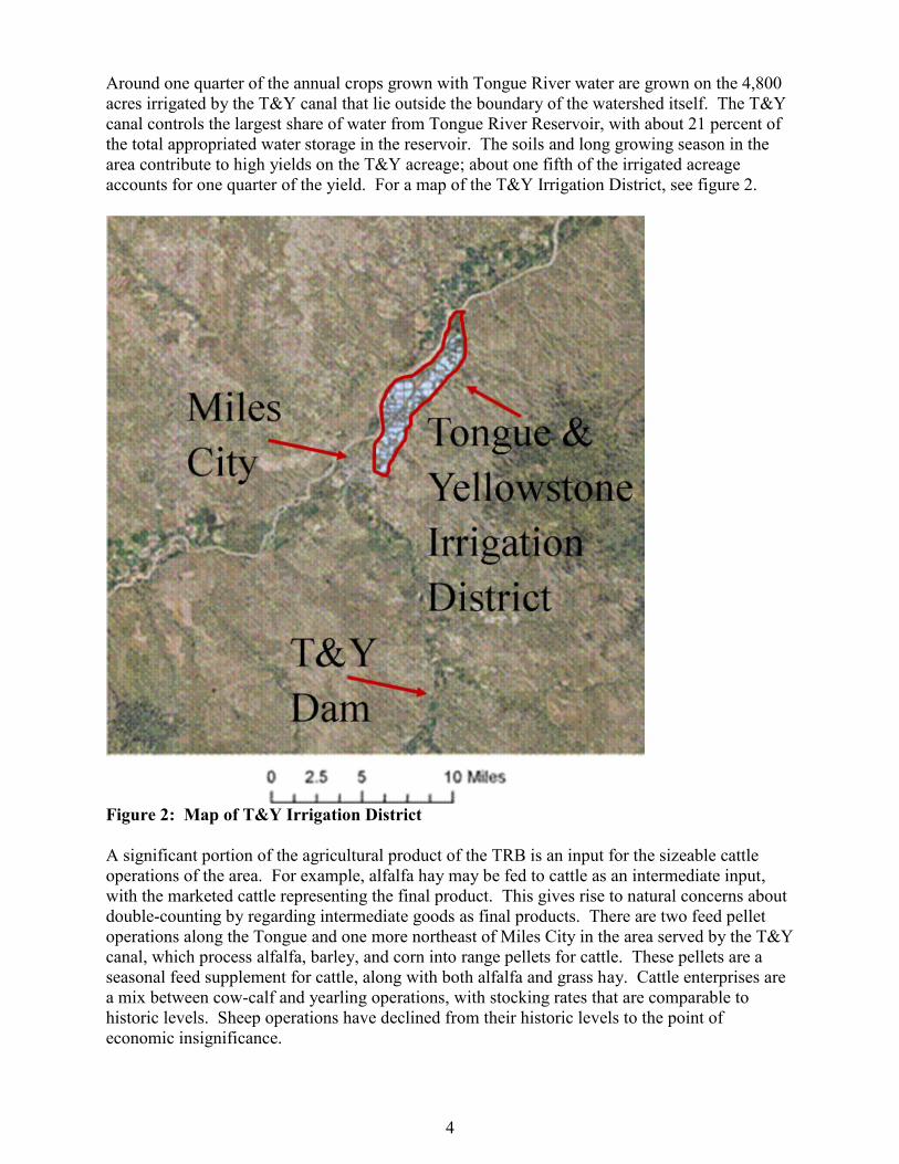
Around one quarter of the annual crops grown with Tongue River water are grown on the 4,800
acres irrigated by the T&Y canal that lie outside the boundary of the watershed itself. The T&Y
canal controls the largest share of water from Tongue River Reservoir, with about 21 percent of
the total appropriated water storage in the reservoir. The soils and long growing season in the
area contribute to high yields on the T&Y acreage; about one fifth of the irrigated acreage
accounts for one quarter of the yield. For a map of the T&Y Irrigation District, see figure 2.
Figure 2: Map of T&Y Irrigation District
A significant portion of the agricultural product of the TRB is an input for the sizeable cattle
operations of the area. For example, alfalfa hay may be fed to cattle as an intermediate input,
with the marketed cattle representing the final product. This gives rise to natural concerns about
double-counting by regarding intermediate goods as final products. There are two feed pellet
operations along the Tongue and one more northeast of Miles City in the area served by the T&Y
canal, which process alfalfa, barley, and corn into range pellets for cattle. These pellets are a
seasonal feed supplement for cattle, along with both alfalfa and grass hay. Cattle enterprises are
a mix between cow-calf and yearling operations, with stocking rates that are comparable to
historic levels. Sheep operations have declined from their historic levels to the point of
economic insignificance.
5
While agriculture is an important portion of the economic base, there are other industries as well.
Two large surface coal mines operate near the state line in the upper drainage, and a third is
located just east of the watershed boundary at Colstrip.3 Due to the proximity to the state line,
some of the economic activity associated with these operations is apportioned to Wyoming,
further complicating the accounting. Federal, state, and local governments are considering
proposals to expand coal mining in the watershed, both in the Otter Creek tributary near Ashland
and near existing operations further south. Expansion of coal production has been the subject of
intense debate.4
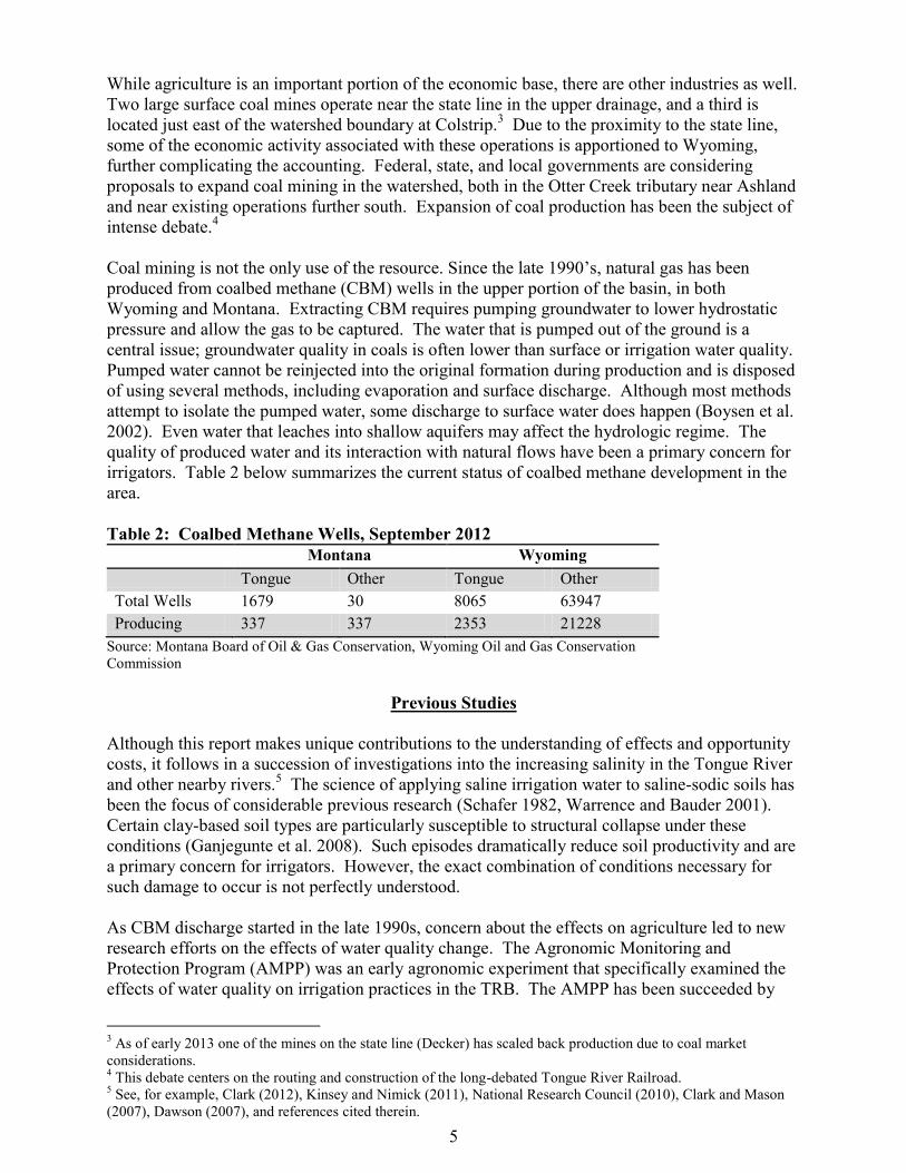
Coal mining is not the only use of the resource. Since the late 1990’s, natural gas has been
produced from coalbed methane (CBM) wells in the upper portion of the basin, in both
Wyoming and Montana. Extracting CBM requires pumping groundwater to lower hydrostatic
pressure and allow the gas to be captured. The water that is pumped out of the ground is a
central issue; groundwater quality in coals is often lower than surface or irrigation water quality.
Pumped water cannot be reinjected into the original formation during production and is disposed
of using several methods, including evaporation and surface discharge. Although most methods
attempt to isolate the pumped water, some discharge to surface water does happen (Boysen et al.
2002). Even water that leaches into shallow aquifers may affect the hydrologic regime. The
quality of produced water and its interaction with natural flows have been a primary concern for
irrigators. Table 2 below summarizes the current status of coalbed methane development in the
area.
Table 2: Coalbed Methane Wells, September 2012
Montana Wyoming
Tongue Other Tongue Other
Total Wells 1679 30 8065 63947
Producing 337 337 2353 21228
Source: Montana Board of Oil & Gas Conservation, Wyoming Oil and Gas Conservation
Commission
Previous Studies
Although this report makes unique contributions to the understanding of effects and opportunity
costs, it follows in a succession of investigations into the increasing salinity in the Tongue River
and other nearby rivers.5 The science of applying saline irrigation water to saline-sodic soils has
been the focus of considerable previous research (Schafer 1982, Warrence and Bauder 2001).
Certain clay-based soil types are particularly susceptible to structural collapse under these
conditions (Ganjegunte et al. 2008). Such episodes dramatically reduce soil productivity and are
a primary concern for irrigators. However, the exact combination of conditions necessary for
such damage to occur is not perfectly understood.
As CBM discharge started in the late 1990s, concern about the effects on agriculture led to new
research efforts on the effects of water quality change. The Agronomic Monitoring and
Protection Program (AMPP) was an early agronomic experiment that specifically examined the
effects of water quality on irrigation practices in the TRB. The AMPP has been succeeded by
3 As of early 2013 one of the mines on the state line (Decker) has scaled back production due to coal market
considerations. 4 This debate centers on the routing and construction of the long-debated Tongue River Railroad.
5 See, for example, Clark (2012), Kinsey and Nimick (2011), National Research Council (2010), Clark and Mason
(2007), Dawson (2007), and references cited therein.

6
the Tongue River Information Project (TRIP).6 The primary conclusion of these plot-level
agronomic studies is that variation in salinity and sodium levels is not correlated with crop yield
differences (Osborne et al. 2010). Drought is implicated as an important cause of the concerns
since water quantity and quality are negatively correlated.
There is a difference of opinion between field studies, which have generally not found significant
impacts of water quality, and lab studies, which have warned against severe impacts from
degraded water quality. Vance et al. (2005) confirm that CBM produced water can alter soil
chemistry by contributing to build-up of salts and sodium in the root zone. Stearns et al. (2005)
examined the effect of direct application on soils and vegetation, and found that the water
degraded both. However, these lab studies may omit important factors such as rainfall, which is
known to interact in complex but important ways with the application of irrigation water (Suarez
et al. 2006). Location and soil type of sites selected for field studies is clearly critical. Producers
have offered anecdotal evidence of yield reductions, especially in the lower reaches of the river.
In addition to initial agronomic trials, the hydrologic connection between surface water,
groundwater, and irrigation is a critical topic for research. The structural links between the three
are not perfectly understood. The hydrologic system in the basin is complicated and not
perfectly understood. Groundwater and surface water flows are related in imperfectly
understood ways that change over the course of the basin. However, by computer simulation of
the basin, long-run impacts on groundwater storage and availability are predicted (Myers 2009).
The interaction between the quality of water and the existing system of water rights is complex.
Irrigators own rights to quantities of water, but the quality of water is generally regulated by
concentration standards.7 In Montana such standards are set by the Water Quality Division of
the Department of Environmental Quality. At this point in time Total Maximum Daily Load
standards have not been set for the Tongue River or Powder River watersheds. So irrigators are
potentially subject to unregulated water quality variation.
AGRICULTURAL PRODUCTION
An important source of information about irrigated agriculture is the Farm and Ranch Irrigation
Survey (FRIS) conducted every 5 years by the USDA with the Census of Agriculture. The most
recent available survey data are from 2008, following the 2007 census. Irrigation is important in
Montana—about 10 percent of the nearly 20 million acres of cropland on farms and ranches in
the state is irrigated—about 1.95 million acres on 8,500 farms.8 The figures for irrigated acreage
have not changed much over successive censuses and total irrigated acreage has been very near 2
million acres for 20 years or more. In aggregate, each year Montana farmers apply 2.66 million
acre-feet of water. Gravity application accounts for about 56 percent of acres irrigated and
sprinklers account for about 44 percent. In the 2008 survey, 12 farms in Montana reported water
quality issues as the main cause of reduced crop yields on a total of 11,496 acres. In contrast,
1,585 farms reported a shortage of water as an issue on a total of 362,461 acres. So low water
quality may be an issue for some producers, but lack of water appears to affect many more
producers. The main irrigated crops by acreage in Montana are shown in Table 3, along with the
average yield gains that irrigation provides.
6 The primary investigators have remained the same but the sponsors of the research have changed from a private
energy developer to the Montana Board of Oil and Gas Conservation. Reports available at:
http://bogc.dnrc.mt.gov/reports.asp . 7 Fitzgerald (2012) explores the issues that this raises for water users, and suggests remedies.
8 Figures are from 2008 Farm and Ranch Irrigation Survey (FRIS):
http://www.agcensus.usda.gov/Publications/2007/Online_Highlights/Farm_and_Ranch_Irrigation_Survey/index.php
7
Summarizing the agricultural productivity of the Tongue River is a challenging task because data
are not collected at the watershed level. So while state or even county-level estimates are readily
available, calculating the production attributable to a specific watershed is more difficult. One
data option is the USDA Census of Agriculture; this census of all agricultural producers in the
United States is conducted every five years. Data are reported on a number of geographic levels,
including at the watershed level. Unfortunately in the case of the Tongue, only two data points
are available for apportioned Census of Agriculture responses—2002 and 2007.9 The responses
also include the production of the Wyoming portion of the basin, without a clear demarcation
between the two. So other data sources are needed to track historical agricultural output.
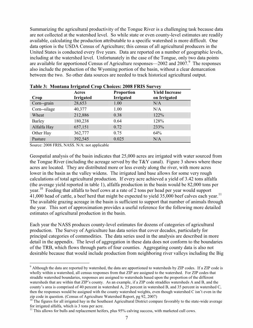
Table 3: Montana Irrigated Crop Choices: 2008 FRIS Survey
Crop
Acres
Irrigated
Proportion
Irrigated
Yield Increase
on Irrigated
Corn--grain 28,653 1.00 N/A
Corn--silage 40,377 1.00 N/A
Wheat 212,886 0.38 122%
Barley 180,238 0.64 128%
Alfalfa Hay 657,151 0.72 233%
Other Hay 362,777 0.75 64%
Pasture 392,545 0.025 N/A
Source: 2008 FRIS, NASS. N/A: not applicable
Geospatial analysis of the basin indicates that 25,000 acres are irrigated with water sourced from
the Tongue River (including the acreage served by the T&Y canal). Figure 3 shows where these
acres are located. They are distributed more or less evenly along the river, with more acres
lower in the basin as the valley widens. The irrigated land base allows for some very rough
calculations of total agricultural production. If every acre achieved a yield of 3.42 tons alfalfa
(the average yield reported in table 1), alfalfa production in the basin would be 82,000 tons per
year.10
Feeding that alfalfa to beef cows at a rate of 2 tons per head per year would support
41,000 head of cattle, a beef herd that might be expected to yield 35,000 beef calves each year.11
The available grazing acreage in the basin is sufficient to support that number of animals through
the year. This sort of approximation provides a useful reference for the following more detailed
estimates of agricultural production in the basin.
Each year the NASS produces county-level estimates for dozens of categories of agricultural
production. The Survey of Agriculture has data series that cover decades, particularly for
principal categories of commodities. The data series used in the analysis are described in more
detail in the appendix. The level of aggregation in these data does not conform to the boundaries
of the TRB, which flows through parts of four counties. Aggregating county data is also not
desirable because that would include production from neighboring river valleys including the Big
9 Although the data are reported by watershed, the data are apportioned to watersheds by ZIP codes. If a ZIP code is
wholly within a watershed, all census responses from that ZIP are assigned to the watershed. For ZIP codes that
straddle watershed boundaries, responses are assigned to watersheds based upon the proportion of the different
watersheds that are within that ZIP’s county. As an example, if a ZIP code straddles watersheds A and B, and the
county’s area is comprised of 40 percent in watershed A, 25 percent in watershed B, and 35 percent in watershed C,
then the responses would be assigned with the county watershed weights, even though watershed C isn’t even in the
zip code in question. (Census of Agriculture Watershed Report, pg 92, 2007) 10
The figures for all irrigated hay in the Southeast Agricultural District compare favorably to the state-wide average
for irrigated alfalfa, which is 3 tons per acre. 11
This allows for bulls and replacement heifers, plus 95% calving success, with marketed cull cows.
8
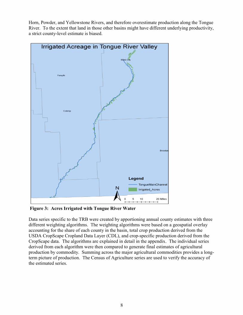
Horn, Powder, and Yellowstone Rivers, and therefore overestimate production along the Tongue
River. To the extent that land in those other basins might have different underlying productivity,
a strict county-level estimate is biased.
Figure 3: Acres Irrigated with Tongue River Water
Data series specific to the TRB were created by apportioning annual county estimates with three
different weighting algorithms. The weighting algorithms were based on a geospatial overlay
accounting for the share of each county in the basin, total crop production derived from the
USDA CropScape Cropland Data Layer (CDL), and crop-specific production derived from the
CropScape data. The algorithms are explained in detail in the appendix. The individual series
derived from each algorithm were then compared to generate final estimates of agricultural
production by commodity. Summing across the major agricultural commodities provides a long-
term picture of production. The Census of Agriculture series are used to verify the accuracy of
the estimated series.
9
Table 4: Montana Price Series for Agricultural Commodities
Year Barley
($/bu)
Cattle-Excl.
Calves ($/cwt)
Corn, Grain
($/bu)
Alfalfa
($/ton)
1980 2.70 58.00 3.60 62.50
1981 2.33 51.90 3.28 48.50
1982 2.06 48.20 2.35 50.00
1983 2.40 48.00 3.20 63.00
1984 2.41 47.20 3.10 78.00
1985 2.03 47.60 2.80 84.50
1986 1.60 49.30 2.10 51.00
1987 1.82 61.10 2.20 45.00
1988 2.82 65.70 3.15 85.00
1989 2.21 68.20 2.60 70.00
1990 2.30 70.60 2.50 65.00
1991 2.34 69.80 2.70 51.50
1992 2.39 66.50 2.50 71.50
1993 2.06 75.60 2.90 69.50
1994 2.22 71.60 2.65 71.50
1995 3.00 59.80 3.00 67.50
1996 3.07 53.80 2.60 81.00
1997 2.83 64.50 2.40 80.00
1998 2.27 62.00 1.90 73.00
1999 2.32 67.60 1.55 66.00
2000 2.38 78.30 1.53 86.50
2001 2.65 80.50 1.89 95.50
2002 2.86 70.50 2.45 85.00
2003 2.93 82.20 2.65 75.00
2004 2.85 91.00 2.42 77.00
2005 2.92 104.00 2.54 71.00
2006 3.00 93.80 3.93 78.00
2007 4.14 89.80 4.76 79.00
2008 5.78 87.50 3.80 117.00
2009 4.86 77.70 4.23 96.00
2010 4.08 90.10 6.00 79.00
Source: NASS. Note: Before 1989 alfalfa hay price is for all hay.
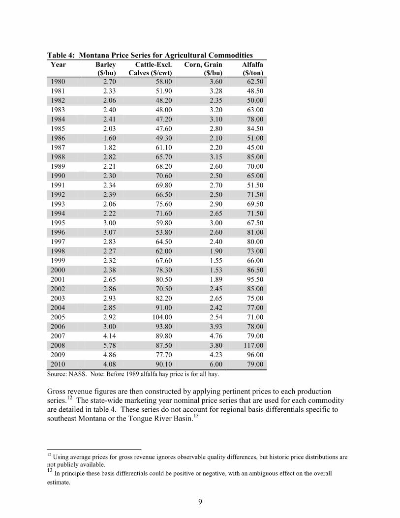
Gross revenue figures are then constructed by applying pertinent prices to each production
series.12
The state-wide marketing year nominal price series that are used for each commodity
are detailed in table 4. These series do not account for regional basis differentials specific to
southeast Montana or the Tongue River Basin.13
12
Using average prices for gross revenue ignores observable quality differences, but historic price distributions are
not publicly available. 13
In principle these basis differentials could be positive or negative, with an ambiguous effect on the overall
estimate.
10
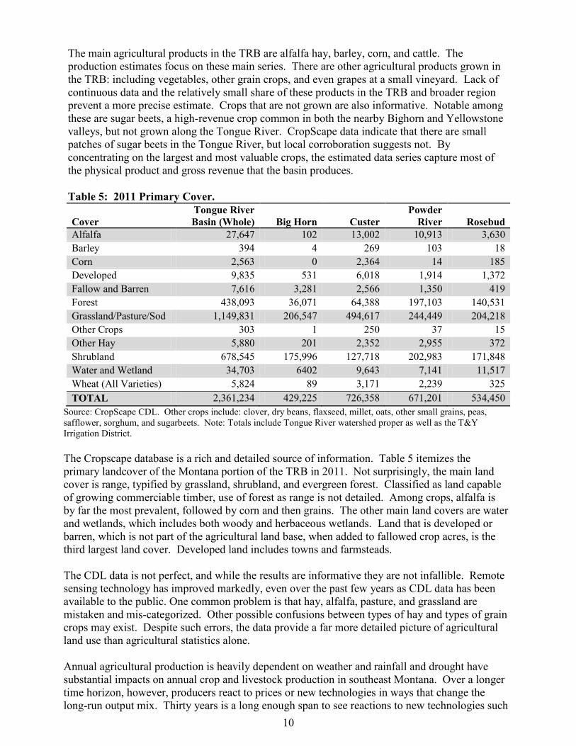
The main agricultural products in the TRB are alfalfa hay, barley, corn, and cattle. The
production estimates focus on these main series. There are other agricultural products grown in
the TRB: including vegetables, other grain crops, and even grapes at a small vineyard. Lack of
continuous data and the relatively small share of these products in the TRB and broader region
prevent a more precise estimate. Crops that are not grown are also informative. Notable among
these are sugar beets, a high-revenue crop common in both the nearby Bighorn and Yellowstone
valleys, but not grown along the Tongue River. CropScape data indicate that there are small
patches of sugar beets in the Tongue River, but local corroboration suggests not. By
concentrating on the largest and most valuable crops, the estimated data series capture most of
the physical product and gross revenue that the basin produces.
Table 5: 2011 Primary Cover.
Cover
Tongue River
Basin (Whole) Big Horn Custer
Powder
River Rosebud
Alfalfa 27,647 102 13,002 10,913 3,630
Barley 394 4 269 103 18
Corn 2,563 0 2,364 14 185
Developed 9,835 531 6,018 1,914 1,372
Fallow and Barren 7,616 3,281 2,566 1,350 419
Forest 438,093 36,071 64,388 197,103 140,531
Grassland/Pasture/Sod 1,149,831 206,547 494,617 244,449 204,218
Other Crops 303 1 250 37 15
Other Hay 5,880 201 2,352 2,955 372
Shrubland 678,545 175,996 127,718 202,983 171,848
Water and Wetland 34,703 6402 9,643 7,141 11,517
Wheat (All Varieties) 5,824 89 3,171 2,239 325
TOTAL 2,361,234 429,225 726,358 671,201 534,450
Source: CropScape CDL. Other crops include: clover, dry beans, flaxseed, millet, oats, other small grains, peas,
safflower, sorghum, and sugarbeets. Note: Totals include Tongue River watershed proper as well as the T&Y
Irrigation District.
The Cropscape database is a rich and detailed source of information. Table 5 itemizes the
primary landcover of the Montana portion of the TRB in 2011. Not surprisingly, the main land
cover is range, typified by grassland, shrubland, and evergreen forest. Classified as land capable
of growing commerciable timber, use of forest as range is not detailed. Among crops, alfalfa is
by far the most prevalent, followed by corn and then grains. The other main land covers are water
and wetlands, which includes both woody and herbaceous wetlands. Land that is developed or
barren, which is not part of the agricultural land base, when added to fallowed crop acres, is the
third largest land cover. Developed land includes towns and farmsteads.
The CDL data is not perfect, and while the results are informative they are not infallible. Remote
sensing technology has improved markedly, even over the past few years as CDL data has been
available to the public. One common problem is that hay, alfalfa, pasture, and grassland are
mistaken and mis-categorized. Other possible confusions between types of hay and types of grain
crops may exist. Despite such errors, the data provide a far more detailed picture of agricultural
land use than agricultural statistics alone.
Annual agricultural production is heavily dependent on weather and rainfall and drought have
substantial impacts on annual crop and livestock production in southeast Montana. Over a longer
time horizon, however, producers react to prices or new technologies in ways that change the
long-run output mix. Thirty years is a long enough span to see reactions to new technologies such
11
as irrigation sprinklers and new seed varieties—and then to have those adoptions fall by the
wayside in favor of new practices. An accurate picture of agricultural in the valley can only be
obtained by accounting for both long- and short-run changes in agricultural production.
Crop Results
Alfalfa
Alfalfa is unusual among field crops in that it is perennial. New seedings and older stands have
lower yields than well-established stands. As a result, stands of alfalfa are renewed every few
years with rotations that vary between 4-10 years. Growing alfalfa requires patience and
prevents farmers from reacting to annual price variations in the ways they are able to with
annually-planted crops. Producers usually plant a small grain crop such as barley or wheat as a
nurse crop to help establish a new alfalfa stand. These nurse crops are sometimes harvested as
hay instead of for grain. Alfalfa can be grown either as a dryland crop or, if water is available, as
an irrigated crop. Alfalfa yields change dramatically when the crop is irrigated (see table 1).
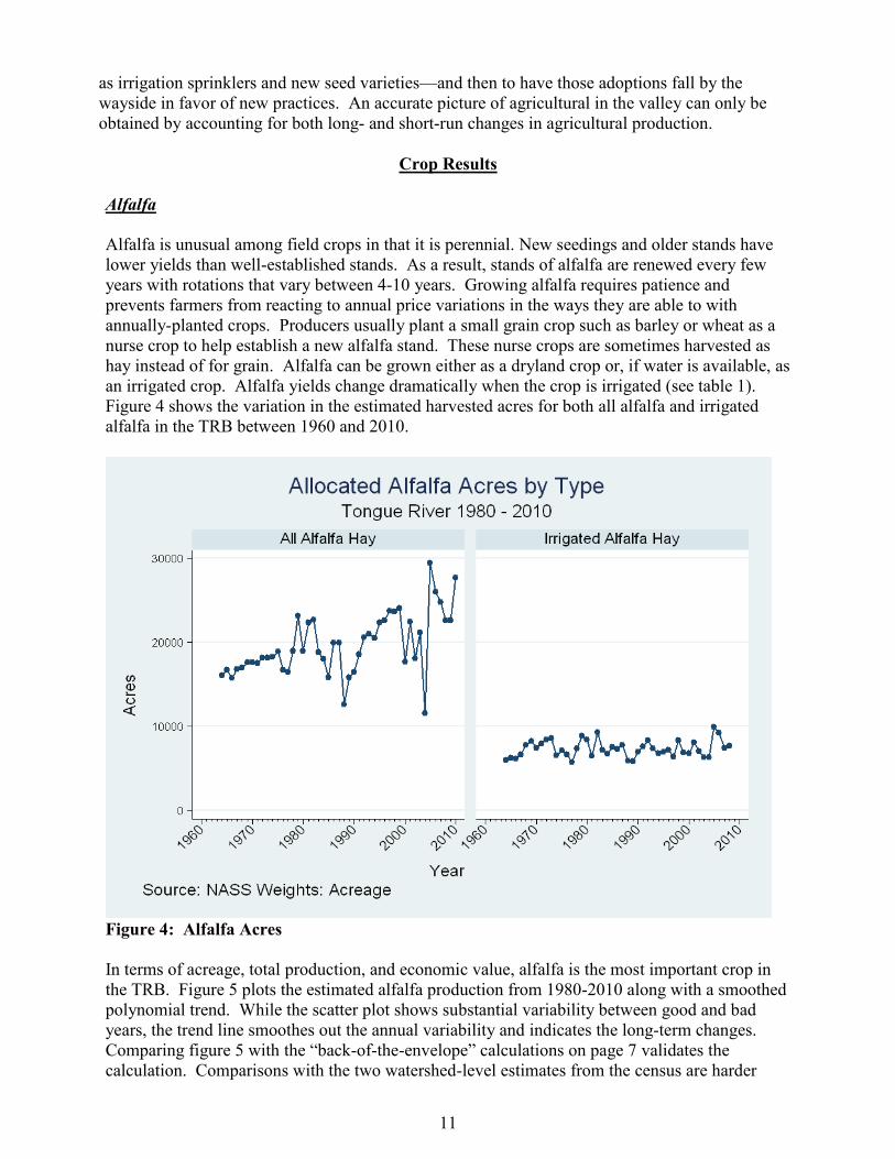
Figure 4 shows the variation in the estimated harvested acres for both all alfalfa and irrigated
alfalfa in the TRB between 1960 and 2010.
Figure 4: Alfalfa Acres
In terms of acreage, total production, and economic value, alfalfa is the most important crop in
the TRB. Figure 5 plots the estimated alfalfa production from 1980-2010 along with a smoothed
polynomial trend. While the scatter plot shows substantial variability between good and bad
years, the trend line smoothes out the annual variability and indicates the long-term changes.
Comparing figure 5 with the “back-of-the-envelope” calculations on page 7 validates the
calculation. Comparisons with the two watershed-level estimates from the census are harder
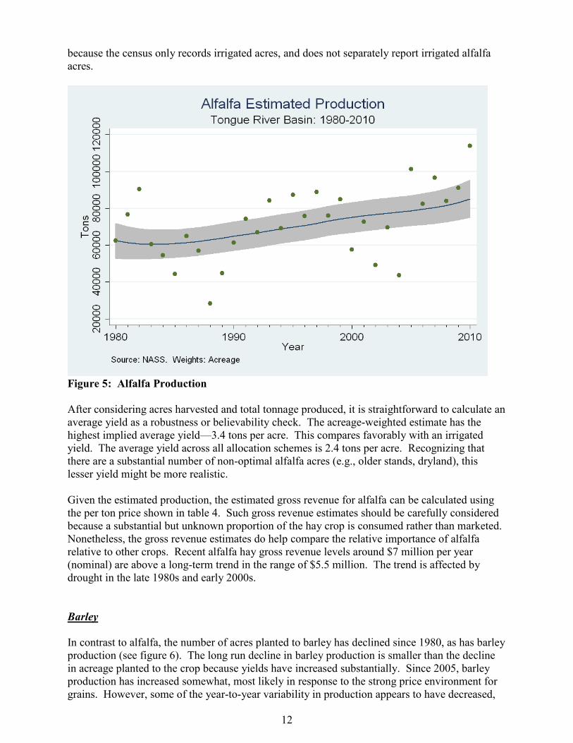
12
because the census only records irrigated acres, and does not separately report irrigated alfalfa
acres.
Figure 5: Alfalfa Production
After considering acres harvested and total tonnage produced, it is straightforward to calculate an
average yield as a robustness or believability check. The acreage-weighted estimate has the
highest implied average yield—3.4 tons per acre. This compares favorably with an irrigated
yield. The average yield across all allocation schemes is 2.4 tons per acre. Recognizing that
there are a substantial number of non-optimal alfalfa acres (e.g., older stands, dryland), this
lesser yield might be more realistic.
Given the estimated production, the estimated gross revenue for alfalfa can be calculated using
the per ton price shown in table 4. Such gross revenue estimates should be carefully considered
because a substantial but unknown proportion of the hay crop is consumed rather than marketed.
Nonetheless, the gross revenue estimates do help compare the relative importance of alfalfa
relative to other crops. Recent alfalfa hay gross revenue levels around $7 million per year
(nominal) are above a long-term trend in the range of $5.5 million. The trend is affected by
drought in the late 1980s and early 2000s.
Barley
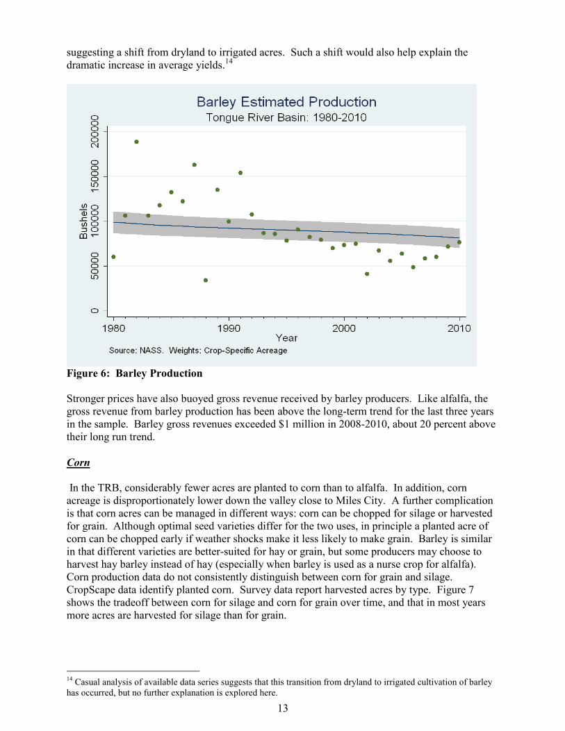
In contrast to alfalfa, the number of acres planted to barley has declined since 1980, as has barley
production (see figure 6). The long run decline in barley production is smaller than the decline
in acreage planted to the crop because yields have increased substantially. Since 2005, barley
production has increased somewhat, most likely in response to the strong price environment for
grains. However, some of the year-to-year variability in production appears to have decreased,
13
suggesting a shift from dryland to irrigated acres. Such a shift would also help explain the
dramatic increase in average yields.14
Figure 6: Barley Production
Stronger prices have also buoyed gross revenue received by barley producers. Like alfalfa, the
gross revenue from barley production has been above the long-term trend for the last three years
in the sample. Barley gross revenues exceeded $1 million in 2008-2010, about 20 percent above
their long run trend.
Corn
In the TRB, considerably fewer acres are planted to corn than to alfalfa. In addition, corn
acreage is disproportionately lower down the valley close to Miles City. A further complication
is that corn acres can be managed in different ways: corn can be chopped for silage or harvested
for grain. Although optimal seed varieties differ for the two uses, in principle a planted acre of
corn can be chopped early if weather shocks make it less likely to make grain. Barley is similar
in that different varieties are better-suited for hay or grain, but some producers may choose to
harvest hay barley instead of hay (especially when barley is used as a nurse crop for alfalfa).
Corn production data do not consistently distinguish between corn for grain and silage.
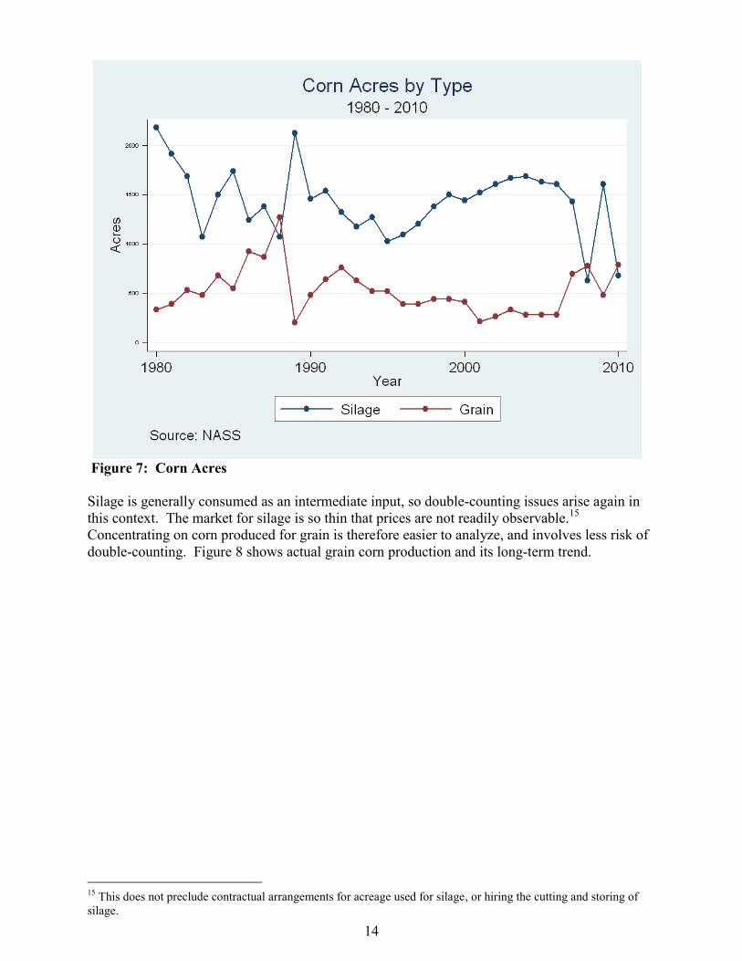
CropScape data identify planted corn. Survey data report harvested acres by type. Figure 7
shows the tradeoff between corn for silage and corn for grain over time, and that in most years
more acres are harvested for silage than for grain.
14
Casual analysis of available data series suggests that this transition from dryland to irrigated cultivation of barley
has occurred, but no further explanation is explored here.
14
Figure 7: Corn Acres
Silage is generally consumed as an intermediate input, so double-counting issues arise again in
this context. The market for silage is so thin that prices are not readily observable.15
Concentrating on corn produced for grain is therefore easier to analyze, and involves less risk of
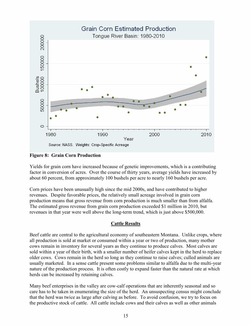
double-counting. Figure 8 shows actual grain corn production and its long-term trend.
15
This does not preclude contractual arrangements for acreage used for silage, or hiring the cutting and storing of
silage.
15
Figure 8: Grain Corn Production
Yields for grain corn have increased because of genetic improvements, which is a contributing
factor in conversion of acres. Over the course of thirty years, average yields have increased by
about 60 percent, from approximately 100 bushels per acre to nearly 160 bushels per acre.
Corn prices have been unusually high since the mid 2000s, and have contributed to higher
revenues. Despite favorable prices, the relatively small acreage involved in grain corn
production means that gross revenue from corn production is much smaller than from alfalfa.
The estimated gross revenue from grain corn production exceeded $1 million in 2010, but
revenues in that year were well above the long-term trend, which is just above $500,000.
Cattle Results
Beef cattle are central to the agricultural economy of southeastern Montana. Unlike crops, where
all production is sold at market or consumed within a year or two of production, many mother
cows remain in inventory for several years as they continue to produce calves. Most calves are
sold within a year of their birth, with a smaller number of heifer calves kept in the herd to replace
older cows. Cows remain in the herd so long as they continue to raise calves; culled animals are
usually marketed. In a sense cattle present some problems similar to alfalfa due to the multi-year
nature of the production process. It is often costly to expand faster than the natural rate at which
herds can be increased by retaining calves.
Many beef enterprises in the valley are cow-calf operations that are inherently seasonal and so
care has to be taken in enumerating the size of the herd. An unsuspecting census might conclude
that the herd was twice as large after calving as before. To avoid confusion, we try to focus on
the productive stock of cattle. All cattle include cows and their calves as well as other animals
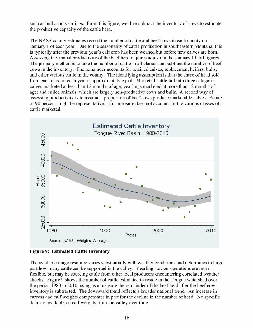
16
such as bulls and yearlings. From this figure, we then subtract the inventory of cows to estimate
the productive capacity of the cattle herd.
The NASS county estimates record the number of cattle and beef cows in each county on
January 1 of each year. Due to the seasonality of cattle production in southeastern Montana, this
is typically after the previous year’s calf crop has been weaned but before new calves are born.
Assessing the annual productivity of the beef herd requires adjusting the January 1 herd figures.
The primary method is to take the number of cattle in all classes and subtract the number of beef
cows in the inventory. The remainder accounts for retained calves, replacement heifers, bulls,
and other various cattle in the county. The identifying assumption is that the share of head sold
from each class in each year is approximately equal. Marketed cattle fall into three categories:
calves marketed at less than 12 months of age; yearlings marketed at more than 12 months of
age; and culled animals, which are largely non-productive cows and bulls. A second way of
assessing productivity is to assume a proportion of beef cows produce marketable calves. A rate
of 90 percent might be representative. This measure does not account for the various classes of
cattle marketed.
Figure 9: Estimated Cattle Inventory
The available range resource varies substantially with weather conditions and determines in large
part how many cattle can be supported in the valley. Yearling stocker operations are more
flexible, but may be sourcing cattle from other local producers encountering correlated weather
shocks. Figure 9 shows the number of cattle estimated to reside in the Tongue watershed over
the period 1980 to 2010, using as a measure the remainder of the beef herd after the beef cow
inventory is subtracted. The downward trend reflects a broader national trend. An increase in
carcass and calf weights compensates in part for the decline in the number of head. No specific
data are available on calf weights from the valley over time.
17
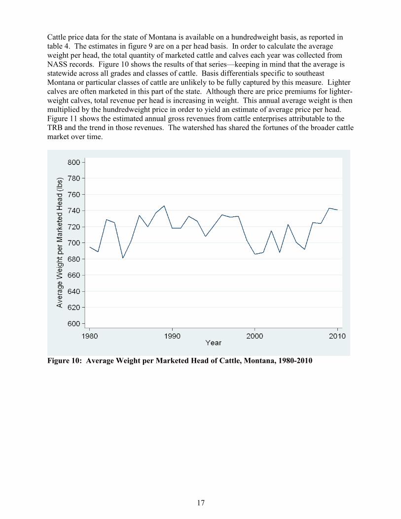
Cattle price data for the state of Montana is available on a hundredweight basis, as reported in
table 4. The estimates in figure 9 are on a per head basis. In order to calculate the average
weight per head, the total quantity of marketed cattle and calves each year was collected from
NASS records. Figure 10 shows the results of that series—keeping in mind that the average is
statewide across all grades and classes of cattle. Basis differentials specific to southeast
Montana or particular classes of cattle are unlikely to be fully captured by this measure. Lighter
calves are often marketed in this part of the state. Although there are price premiums for lighter-
weight calves, total revenue per head is increasing in weight. This annual average weight is then
multiplied by the hundredweight price in order to yield an estimate of average price per head.
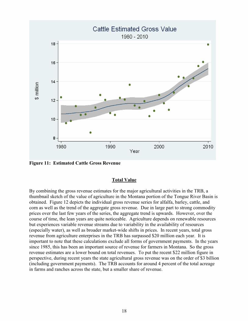
Figure 11 shows the estimated annual gross revenues from cattle enterprises attributable to the
TRB and the trend in those revenues. The watershed has shared the fortunes of the broader cattle
market over time.
Figure 10: Average Weight per Marketed Head of Cattle, Montana, 1980-2010
18
Figure 11: Estimated Cattle Gross Revenue
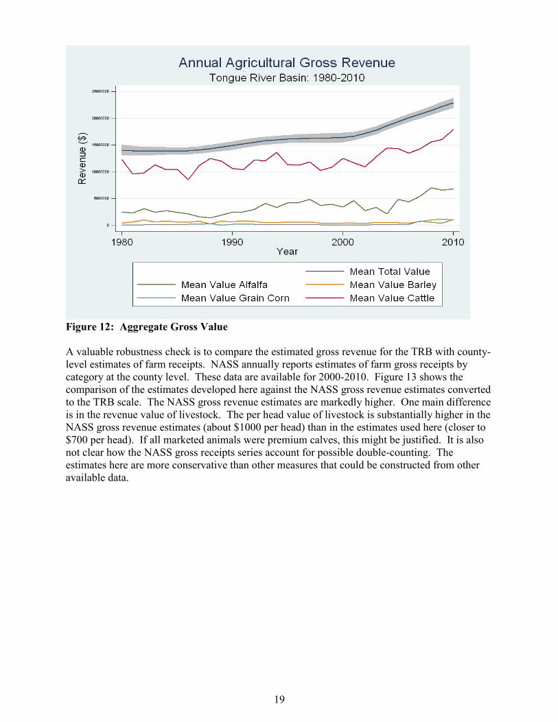
Total Value
By combining the gross revenue estimates for the major agricultural activities in the TRB, a
thumbnail sketch of the value of agriculture in the Montana portion of the Tongue River Basin is
obtained. Figure 12 depicts the individual gross revenue series for alfalfa, barley, cattle, and
corn as well as the trend of the aggregate gross revenue. Due in large part to strong commodity
prices over the last few years of the series, the aggregate trend is upwards. However, over the
course of time, the lean years are quite noticeable. Agriculture depends on renewable resources
but experiences variable revenue streams due to variability in the availability of resources
(especially water), as well as broader market-wide shifts in prices. In recent years, total gross
revenue from agriculture enterprises in the TRB has surpassed $20 million each year. It is
important to note that these calculations exclude all forms of government payments. In the years
since 1985, this has been an important source of revenue for farmers in Montana. So the gross
revenue estimates are a lower bound on total revenues. To put the recent $22 million figure in
perspective, during recent years the state agricultural gross revenue was on the order of $3 billion
(including government payments). The TRB accounts for around 4 percent of the total acreage
in farms and ranches across the state, but a smaller share of revenue.
19
Figure 12: Aggregate Gross Value
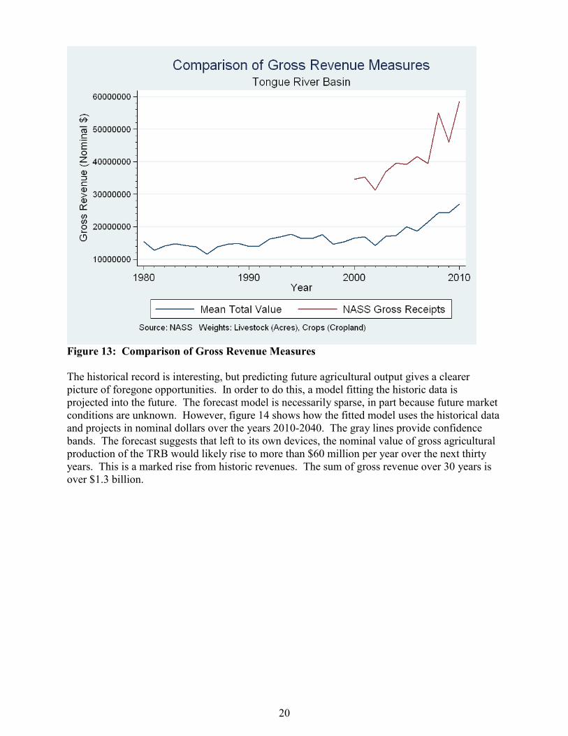
A valuable robustness check is to compare the estimated gross revenue for the TRB with county-
level estimates of farm receipts. NASS annually reports estimates of farm gross receipts by
category at the county level. These data are available for 2000-2010. Figure 13 shows the
comparison of the estimates developed here against the NASS gross revenue estimates converted
to the TRB scale. The NASS gross revenue estimates are markedly higher. One main difference
is in the revenue value of livestock. The per head value of livestock is substantially higher in the
NASS gross revenue estimates (about $1000 per head) than in the estimates used here (closer to
$700 per head). If all marketed animals were premium calves, this might be justified. It is also
not clear how the NASS gross receipts series account for possible double-counting. The
estimates here are more conservative than other measures that could be constructed from other
available data.
20
Figure 13: Comparison of Gross Revenue Measures
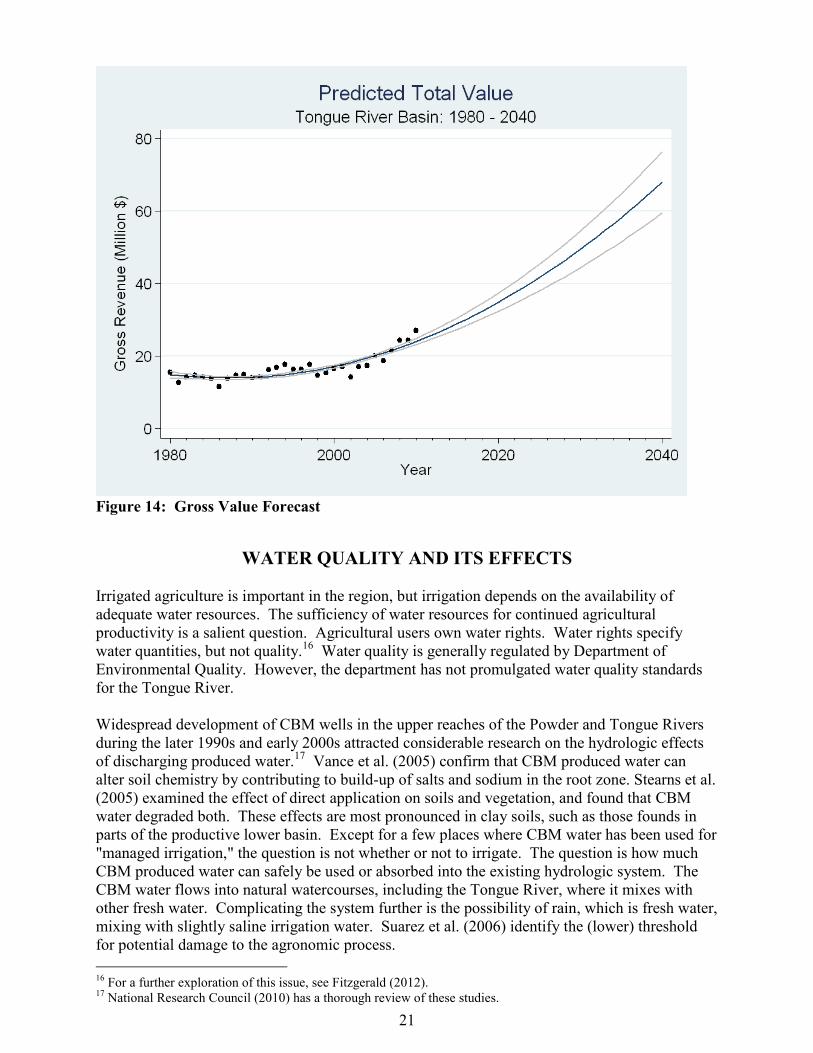
The historical record is interesting, but predicting future agricultural output gives a clearer
picture of foregone opportunities. In order to do this, a model fitting the historic data is
projected into the future. The forecast model is necessarily sparse, in part because future market
conditions are unknown. However, figure 14 shows how the fitted model uses the historical data
and projects in nominal dollars over the years 2010-2040. The gray lines provide confidence
bands. The forecast suggests that left to its own devices, the nominal value of gross agricultural
production of the TRB would likely rise to more than $60 million per year over the next thirty
years. This is a marked rise from historic revenues. The sum of gross revenue over 30 years is
over $1.3 billion.
21
Figure 14: Gross Value Forecast
WATER QUALITY AND ITS EFFECTS
Irrigated agriculture is important in the region, but irrigation depends on the availability of
adequate water resources. The sufficiency of water resources for continued agricultural
productivity is a salient question. Agricultural users own water rights. Water rights specify
water quantities, but not quality.16
Water quality is generally regulated by Department of
Environmental Quality. However, the department has not promulgated water quality standards
for the Tongue River.
Widespread development of CBM wells in the upper reaches of the Powder and Tongue Rivers
during the later 1990s and early 2000s attracted considerable research on the hydrologic effects
of discharging produced water.17
Vance et al. (2005) confirm that CBM produced water can
alter soil chemistry by contributing to build-up of salts and sodium in the root zone. Stearns et al.
(2005) examined the effect of direct application on soils and vegetation, and found that CBM
water degraded both. These effects are most pronounced in clay soils, such as those founds in
parts of the productive lower basin. Except for a few places where CBM water has been used for
"managed irrigation," the question is not whether or not to irrigate. The question is how much
CBM produced water can safely be used or absorbed into the existing hydrologic system. The
CBM water flows into natural watercourses, including the Tongue River, where it mixes with
other fresh water. Complicating the system further is the possibility of rain, which is fresh water,
mixing with slightly saline irrigation water. Suarez et al. (2006) identify the (lower) threshold
for potential damage to the agronomic process.
16
For a further exploration of this issue, see Fitzgerald (2012). 17
National Research Council (2010) has a thorough review of these studies.
22
A number of measures can be used to account for the quality of irrigation water, but two that
account for salinity are the sodium absorption ratio (SAR) and specific conductance (SC).
Taking into account the effects of different types of salts, SAR is a calculated ratio of the
concentration of sodium (Na) ions to calcium (Ca) and magnesium (Mg) ions. While all three
elements are potentially harmful to crops and soils, the calculation of SAR accounts for the
greater impact of sodium. More dissolved salts increase SC, giving a complementary measure of
salinity.
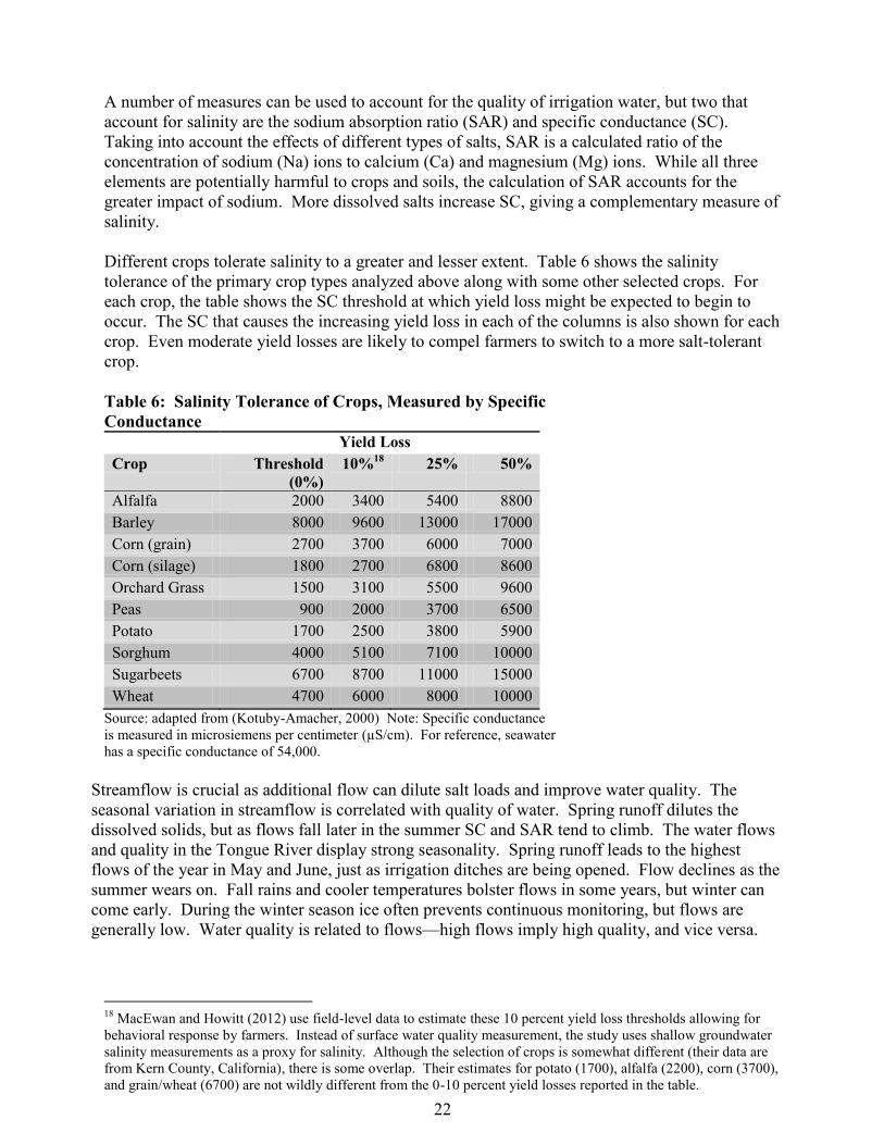
Different crops tolerate salinity to a greater and lesser extent. Table 6 shows the salinity
tolerance of the primary crop types analyzed above along with some other selected crops. For
each crop, the table shows the SC threshold at which yield loss might be expected to begin to
occur. The SC that causes the increasing yield loss in each of the columns is also shown for each
crop. Even moderate yield losses are likely to compel farmers to switch to a more salt-tolerant
crop.
Table 6: Salinity Tolerance of Crops, Measured by Specific
Conductance
Yield Loss
Crop Threshold
(0%)
10%18
25% 50%
Alfalfa 2000 3400 5400 8800
Barley 8000 9600 13000 17000
Corn (grain) 2700 3700 6000 7000
Corn (silage) 1800 2700 6800 8600
Orchard Grass 1500 3100 5500 9600
Peas 900 2000 3700 6500
Potato 1700 2500 3800 5900
Sorghum 4000 5100 7100 10000
Sugarbeets 6700 8700 11000 15000
Wheat 4700 6000 8000 10000
Source: adapted from (Kotuby-Amacher, 2000) Note: Specific conductance
is measured in microsiemens per centimeter (µS/cm). For reference, seawater
has a specific conductance of 54,000.
Streamflow is crucial as additional flow can dilute salt loads and improve water quality. The
seasonal variation in streamflow is correlated with quality of water. Spring runoff dilutes the
dissolved solids, but as flows fall later in the summer SC and SAR tend to climb. The water flows
and quality in the Tongue River display strong seasonality. Spring runoff leads to the highest
flows of the year in May and June, just as irrigation ditches are being opened. Flow declines as the
summer wears on. Fall rains and cooler temperatures bolster flows in some years, but winter can
come early. During the winter season ice often prevents continuous monitoring, but flows are
generally low. Water quality is related to flows—high flows imply high quality, and vice versa.
18
MacEwan and Howitt (2012) use field-level data to estimate these 10 percent yield loss thresholds allowing for
behavioral response by farmers. Instead of surface water quality measurement, the study uses shallow groundwater
salinity measurements as a proxy for salinity. Although the selection of crops is somewhat different (their data are
from Kern County, California), there is some overlap. Their estimates for potato (1700), alfalfa (2200), corn (3700),
and grain/wheat (6700) are not wildly different from the 0-10 percent yield losses reported in the table.

23
Data
The United States Geological Survey (USGS) monitors water quality and flows at a number of
locations along the Tongue River. Two types of records are available in the historical data records.
The first are automated reports from monitoring stations. These stations gather detailed
information about flow and water quality. Because the monitoring equipment is relatively
compact, and the perceptions of where data are most needed have changed over time, the location
of monitoring sites changes over time. Data continuity is not aided by this flexibility. The
complex hydrology of the river means that flows and quality can change in ways that are hard to
understand as a monitoring site is moved up or down stream.
A second type of observations is field studies, which are conducted by hand at various locations
along the river. These observations can help fill in the missing periods of time in the record from
fixed site remote sensors. The set of locations where the USGS currently has monitoring stations
is depicted in Figure 15.
Figure 15: USGS Water Monitoring Sites
Source: USGS
24
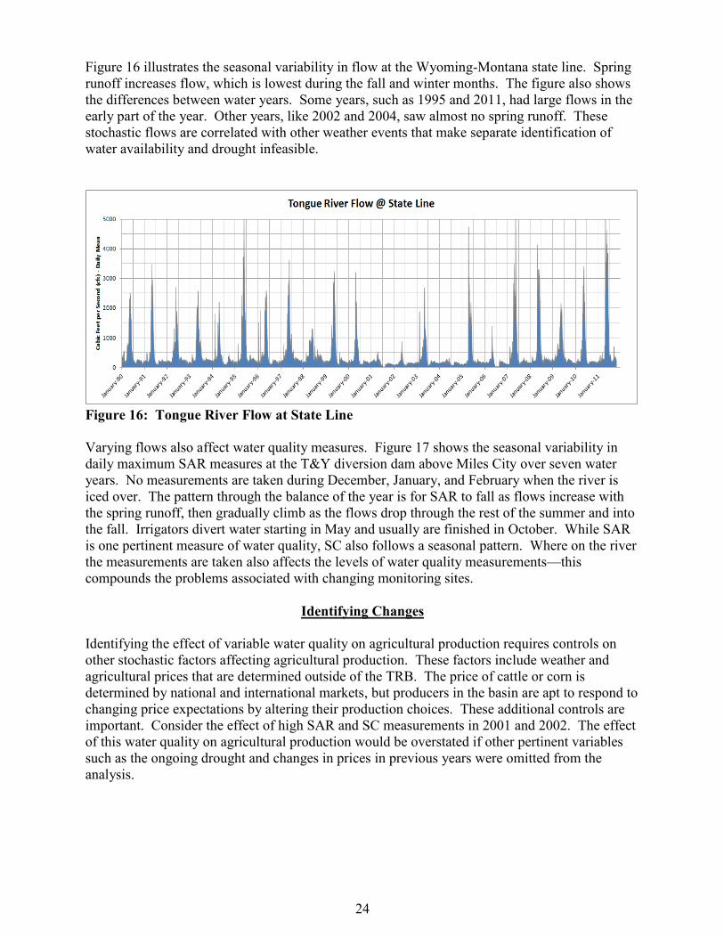
Figure 16 illustrates the seasonal variability in flow at the Wyoming-Montana state line. Spring
runoff increases flow, which is lowest during the fall and winter months. The figure also shows
the differences between water years. Some years, such as 1995 and 2011, had large flows in the
early part of the year. Other years, like 2002 and 2004, saw almost no spring runoff. These
stochastic flows are correlated with other weather events that make separate identification of
water availability and drought infeasible.
Figure 16: Tongue River Flow at State Line
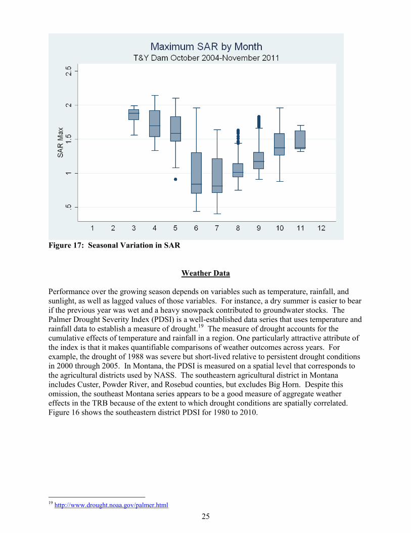
Varying flows also affect water quality measures. Figure 17 shows the seasonal variability in
daily maximum SAR measures at the T&Y diversion dam above Miles City over seven water
years. No measurements are taken during December, January, and February when the river is
iced over. The pattern through the balance of the year is for SAR to fall as flows increase with
the spring runoff, then gradually climb as the flows drop through the rest of the summer and into
the fall. Irrigators divert water starting in May and usually are finished in October. While SAR
is one pertinent measure of water quality, SC also follows a seasonal pattern. Where on the river
the measurements are taken also affects the levels of water quality measurements—this
compounds the problems associated with changing monitoring sites.
Identifying Changes
Identifying the effect of variable water quality on agricultural production requires controls on
other stochastic factors affecting agricultural production. These factors include weather and
agricultural prices that are determined outside of the TRB. The price of cattle or corn is
determined by national and international markets, but producers in the basin are apt to respond to
changing price expectations by altering their production choices. These additional controls are
important. Consider the effect of high SAR and SC measurements in 2001 and 2002. The effect
of this water quality on agricultural production would be overstated if other pertinent variables
such as the ongoing drought and changes in prices in previous years were omitted from the
analysis.
25
Figure 17: Seasonal Variation in SAR
Weather Data
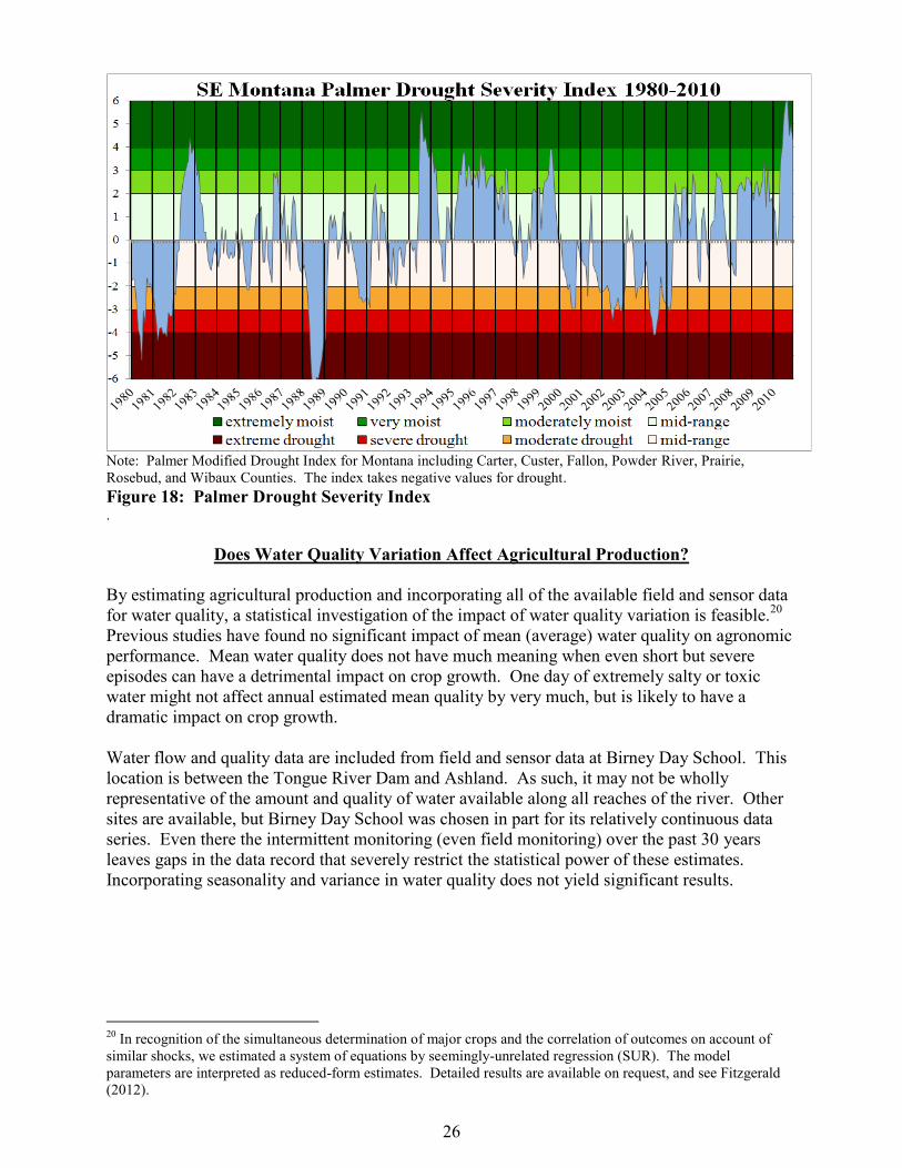
Performance over the growing season depends on variables such as temperature, rainfall, and
sunlight, as well as lagged values of those variables. For instance, a dry summer is easier to bear
if the previous year was wet and a heavy snowpack contributed to groundwater stocks. The
Palmer Drought Severity Index (PDSI) is a well-established data series that uses temperature and
rainfall data to establish a measure of drought.19
The measure of drought accounts for the
cumulative effects of temperature and rainfall in a region. One particularly attractive attribute of
the index is that it makes quantifiable comparisons of weather outcomes across years. For
example, the drought of 1988 was severe but short-lived relative to persistent drought conditions
in 2000 through 2005. In Montana, the PDSI is measured on a spatial level that corresponds to
the agricultural districts used by NASS. The southeastern agricultural district in Montana
includes Custer, Powder River, and Rosebud counties, but excludes Big Horn. Despite this
omission, the southeast Montana series appears to be a good measure of aggregate weather
effects in the TRB because of the extent to which drought conditions are spatially correlated.
Figure 16 shows the southeastern district PDSI for 1980 to 2010.
19
http://www.drought.noaa.gov/palmer.html
26
Note: Palmer Modified Drought Index for Montana including Carter, Custer, Fallon, Powder River, Prairie,
Rosebud, and Wibaux Counties. The index takes negative values for drought. Figure 18: Palmer Drought Severity Index
.
Does Water Quality Variation Affect Agricultural Production?
By estimating agricultural production and incorporating all of the available field and sensor data
for water quality, a statistical investigation of the impact of water quality variation is feasible.20
Previous studies have found no significant impact of mean (average) water quality on agronomic
performance. Mean water quality does not have much meaning when even short but severe
episodes can have a detrimental impact on crop growth. One day of extremely salty or toxic
water might not affect annual estimated mean quality by very much, but is likely to have a
dramatic impact on crop growth.
Water flow and quality data are included from field and sensor data at Birney Day School. This
location is between the Tongue River Dam and Ashland. As such, it may not be wholly
representative of the amount and quality of water available along all reaches of the river. Other
sites are available, but Birney Day School was chosen in part for its relatively continuous data
series. Even there the intermittent monitoring (even field monitoring) over the past 30 years
leaves gaps in the data record that severely restrict the statistical power of these estimates.
Incorporating seasonality and variance in water quality does not yield significant results.
20
In recognition of the simultaneous determination of major crops and the correlation of outcomes on account of
similar shocks, we estimated a system of equations by seemingly-unrelated regression (SUR). The model
parameters are interpreted as reduced-form estimates. Detailed results are available on request, and see Fitzgerald
(2012).
27
DISTRIBUTIONAL IMPLICATIONS
Soils
One of the primary concerns about water quality change is that low-quality irrigation water can
permanently damage certain soils. In addition to the measurements of water quality along the
river, the distribution of soil types on irrigated acreage informs the potential distribution of
impacts. While the full set of risk factors for damage is not perfectly understood, soil type is
recognized as an important piece of the puzzle. Rainfall, cultivation and irrigation history, and
application timing also contribute. The following is a coarse analysis of the soil distribution and
the impacts that it is likely to have on agricultural production.
Irrigation and Soil Type
According to the Soil Survey Geographic Database maintained by the Natural Resources
Conservation Service, the irrigated acreage along the Tongue River has 160 different soil series.
A single field often contains multiple soil series. While differences between some series are
minor, others represent very different soil types. Some soil series are complex, meaning that
multiple soils are mixed. The county-level soil series definitions are not entirely consistent,
which complicates the analysis. An ideal analysis would characterize each soil along pertinent
soil characteristics such as sodicity, particle size, water capacity, and depth.
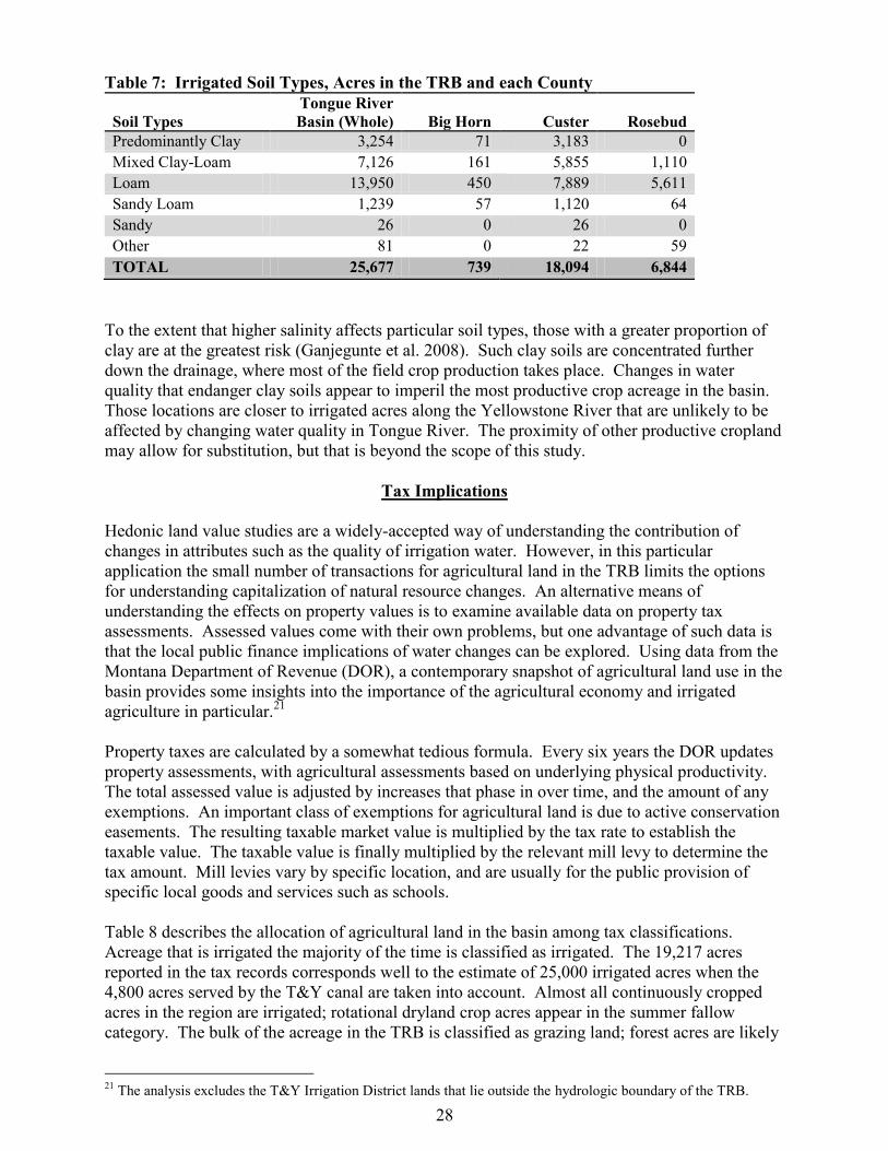
Soils are binned into six categories, as specified in table A6 in the appendix. These
classifications are quite simple: predominantly clay, mixed clay-loam or clayey loam, loam,
sandy loam, sandy, and other. Table 7 shows the number of acres in each of these
classifications. The irrigated acreages are reported by soil type and county. Because Powder
River County does not have the main stem of the Tongue, the county categories effectively
partition the valley into upper (Big Horn), middle (Rosebud), and lower (Custer) sub-basins.
Most of the clay soils are concentrated further down the river, in Custer County and especially in
the T&Y Irrigation District.
Application technology is likely to affect the interaction between soil type and water quality as
well. The 7,781 acres irrigated with center pivot sprinklers are concentrated on clay-loam and
loam soil types, with less than 1,000 acres irrigated by pivot in the predominantly clay category.
The other irrigated acres are not categorized by application technology.
Differences along the river are captured in table 7. The first column summarizes the irrigated
acreage for the whole TRB. The other columns detail the irrigated soil types by county. Note
that this table only details acres irrigated with water from the Tongue, not tributaries. As a
further illustration, the 4,764 acres watered by the T&Y canal outside of the watershed proper
are the lowest area that uses water from the Tongue River. This region has a higher percentage
of soil types that are predominantly clay. The predominantly clay and clay-loam categories
account for 2,793 of the acres, with loam most of the balance.
28
Table 7: Irrigated Soil Types, Acres in the TRB and each County
Soil Types
Tongue River
Basin (Whole) Big Horn Custer Rosebud
Predominantly Clay 3,254 71 3,183 0
Mixed Clay-Loam 7,126 161 5,855 1,110
Loam 13,950 450 7,889 5,611
Sandy Loam 1,239 57 1,120 64
Sandy 26 0 26 0
Other 81 0 22 59
TOTAL 25,677 739 18,094 6,844
To the extent that higher salinity affects particular soil types, those with a greater proportion of
clay are at the greatest risk (Ganjegunte et al. 2008). Such clay soils are concentrated further
down the drainage, where most of the field crop production takes place. Changes in water
quality that endanger clay soils appear to imperil the most productive crop acreage in the basin.
Those locations are closer to irrigated acres along the Yellowstone River that are unlikely to be
affected by changing water quality in Tongue River. The proximity of other productive cropland
may allow for substitution, but that is beyond the scope of this study.
Tax Implications
Hedonic land value studies are a widely-accepted way of understanding the contribution of
changes in attributes such as the quality of irrigation water. However, in this particular
application the small number of transactions for agricultural land in the TRB limits the options
for understanding capitalization of natural resource changes. An alternative means of
understanding the effects on property values is to examine available data on property tax
assessments. Assessed values come with their own problems, but one advantage of such data is
that the local public finance implications of water changes can be explored. Using data from the
Montana Department of Revenue (DOR), a contemporary snapshot of agricultural land use in the
basin provides some insights into the importance of the agricultural economy and irrigated
agriculture in particular.21
Property taxes are calculated by a somewhat tedious formula. Every six years the DOR updates
property assessments, with agricultural assessments based on underlying physical productivity.
The total assessed value is adjusted by increases that phase in over time, and the amount of any
exemptions. An important class of exemptions for agricultural land is due to active conservation
easements. The resulting taxable market value is multiplied by the tax rate to establish the
taxable value. The taxable value is finally multiplied by the relevant mill levy to determine the
tax amount. Mill levies vary by specific location, and are usually for the public provision of
specific local goods and services such as schools.
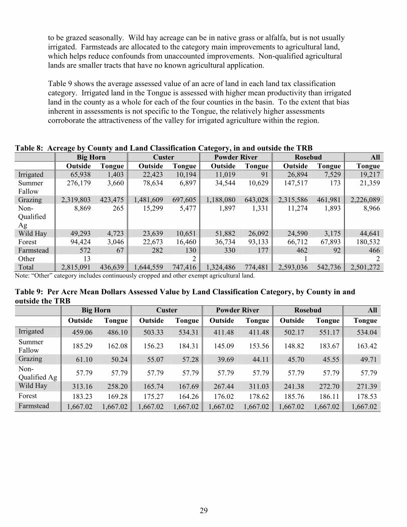
Table 8 describes the allocation of agricultural land in the basin among tax classifications.
Acreage that is irrigated the majority of the time is classified as irrigated. The 19,217 acres
reported in the tax records corresponds well to the estimate of 25,000 irrigated acres when the
4,800 acres served by the T&Y canal are taken into account. Almost all continuously cropped
acres in the region are irrigated; rotational dryland crop acres appear in the summer fallow
category. The bulk of the acreage in the TRB is classified as grazing land; forest acres are likely
21
The analysis excludes the T&Y Irrigation District lands that lie outside the hydrologic boundary of the TRB.
29
to be grazed seasonally. Wild hay acreage can be in native grass or alfalfa, but is not usually
irrigated. Farmsteads are allocated to the category main improvements to agricultural land,
which helps reduce confounds from unaccounted improvements. Non-qualified agricultural
lands are smaller tracts that have no known agricultural application.
Table 9 shows the average assessed value of an acre of land in each land tax classification
category. Irrigated land in the Tongue is assessed with higher mean productivity than irrigated
land in the county as a whole for each of the four counties in the basin. To the extent that bias
inherent in assessments is not specific to the Tongue, the relatively higher assessments
corroborate the attractiveness of the valley for irrigated agriculture within the region.
Table 8: Acreage by County and Land Classification Category, in and outside the TRB
Big Horn Custer Powder River Rosebud All
Outside Tongue Outside Tongue Outside Tongue Outside Tongue Tongue
Irrigated 65,938 1,403 22,423 10,194 11,019 91 26,894 7,529 19,217
Summer
Fallow
276,179 3,660 78,634 6,897 34,544 10,629 147,517 173 21,359
Grazing 2,319,803 423,475 1,481,609 697,605 1,188,080 643,028 2,315,586 461,981 2,226,089
Non-
Qualified
Ag
8,869 265 15,299 5,477 1,897 1,331 11,274 1,893 8,966
Wild Hay 49,293 4,723 23,639 10,651 51,882 26,092 24,590 3,175 44,641
Forest 94,424 3,046 22,673 16,460 36,734 93,133 66,712 67,893 180,532
Farmstead 572 67 282 130 330 177 462 92 466
Other 13 2 1 2
Total 2,815,091 436,639 1,644,559 747,416 1,324,486 774,481 2,593,036 542,736 2,501,272 Note: “Other” category includes continuously cropped and other exempt agricultural land.
Table 9: Per Acre Mean Dollars Assessed Value by Land Classification Category, by County in and
outside the TRB
Big Horn Custer Powder River Rosebud All
Outside Tongue Outside Tongue Outside Tongue Outside Tongue Tongue
Irrigated 459.06 486.10 503.33 534.31 411.48 411.48 502.17 551.17 534.04
Summer
Fallow 185.29 162.08 156.23 184.31 145.09 153.56 148.82 183.67 163.42
Grazing 61.10 50.24 55.07 57.28 39.69 44.11 45.70 45.55 49.71
Non-
Qualified Ag 57.79 57.79 57.79 57.79 57.79 57.79 57.79 57.79 57.79
Wild Hay 313.16 258.20 165.74 167.69 267.44 311.03 241.38 272.70 271.39
Forest 183.23 169.28 175.27 164.26 176.02 178.62 185.76 186.11 178.53
Farmstead 1,667.02 1,667.02 1,667.02 1,667.02 1,667.02 1,667.02 1,667.02 1,667.02 1,667.02
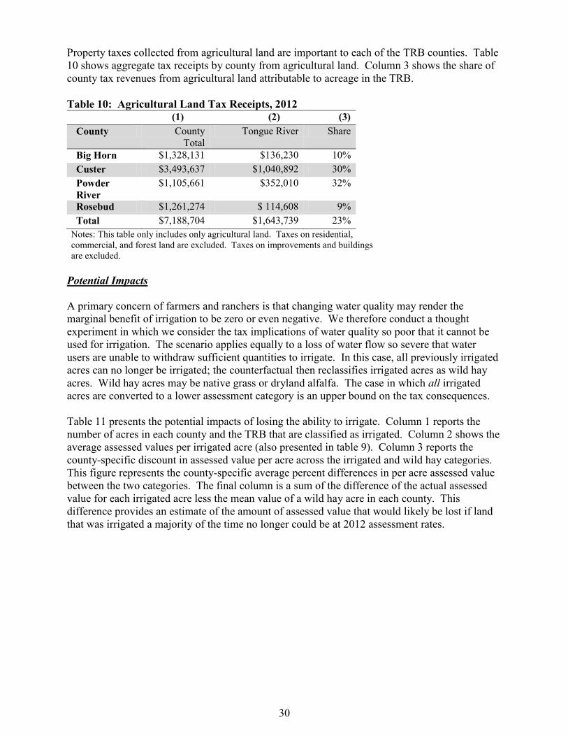
30
Property taxes collected from agricultural land are important to each of the TRB counties. Table
10 shows aggregate tax receipts by county from agricultural land. Column 3 shows the share of
county tax revenues from agricultural land attributable to acreage in the TRB.
Table 10: Agricultural Land Tax Receipts, 2012
(1) (2) (3)
County County
Total
Tongue River Share
Big Horn $1,328,131 $136,230 10%
Custer $3,493,637 $1,040,892 30%
Powder
River
$1,105,661 $352,010 32%
Rosebud $1,261,274 $ 114,608 9%
Total $7,188,704 $1,643,739 23%
Notes: This table only includes only agricultural land. Taxes on residential,
commercial, and forest land are excluded. Taxes on improvements and buildings
are excluded.
Potential Impacts
A primary concern of farmers and ranchers is that changing water quality may render the
marginal benefit of irrigation to be zero or even negative. We therefore conduct a thought
experiment in which we consider the tax implications of water quality so poor that it cannot be
used for irrigation. The scenario applies equally to a loss of water flow so severe that water
users are unable to withdraw sufficient quantities to irrigate. In this case, all previously irrigated
acres can no longer be irrigated; the counterfactual then reclassifies irrigated acres as wild hay
acres. Wild hay acres may be native grass or dryland alfalfa. The case in which all irrigated
acres are converted to a lower assessment category is an upper bound on the tax consequences.
Table 11 presents the potential impacts of losing the ability to irrigate. Column 1 reports the
number of acres in each county and the TRB that are classified as irrigated. Column 2 shows the
average assessed values per irrigated acre (also presented in table 9). Column 3 reports the
county-specific discount in assessed value per acre across the irrigated and wild hay categories.
This figure represents the county-specific average percent differences in per acre assessed value
between the two categories. The final column is a sum of the difference of the actual assessed
value for each irrigated acre less the mean value of a wild hay acre in each county. This
difference provides an estimate of the amount of assessed value that would likely be lost if land
that was irrigated a majority of the time no longer could be at 2012 assessment rates.
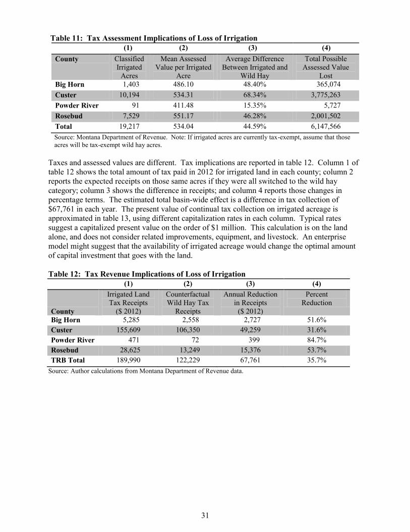
31
Table 11: Tax Assessment Implications of Loss of Irrigation
(1) (2) (3) (4)
County Classified
Irrigated
Acres
Mean Assessed
Value per Irrigated
Acre
Average Difference
Between Irrigated and
Wild Hay
Total Possible
Assessed Value
Lost
Big Horn 1,403 486.10 48.40% 365,074
Custer 10,194 534.31 68.34% 3,775,263
Powder River 91 411.48 15.35% 5,727
Rosebud 7,529 551.17 46.28% 2,001,502
Total 19,217 534.04 44.59% 6,147,566
Source: Montana Department of Revenue. Note: If irrigated acres are currently tax-exempt, assume that those
acres will be tax-exempt wild hay acres.
Taxes and assessed values are different. Tax implications are reported in table 12. Column 1 of
table 12 shows the total amount of tax paid in 2012 for irrigated land in each county; column 2
reports the expected receipts on those same acres if they were all switched to the wild hay
category; column 3 shows the difference in receipts; and column 4 reports those changes in
percentage terms. The estimated total basin-wide effect is a difference in tax collection of
$67,761 in each year. The present value of continual tax collection on irrigated acreage is
approximated in table 13, using different capitalization rates in each column. Typical rates
suggest a capitalized present value on the order of $1 million. This calculation is on the land
alone, and does not consider related improvements, equipment, and livestock. An enterprise
model might suggest that the availability of irrigated acreage would change the optimal amount
of capital investment that goes with the land.
Table 12: Tax Revenue Implications of Loss of Irrigation
(1) (2) (3) (4)
County
Irrigated Land
Tax Receipts
($ 2012)
Counterfactual
Wild Hay Tax
Receipts
Annual Reduction
in Receipts
($ 2012)
Percent
Reduction
Big Horn 5,285 2,558 2,727 51.6%
Custer 155,609 106,350 49,259 31.6%
Powder River 471 72 399 84.7%
Rosebud 28,625 13,249 15,376 53.7%
TRB Total 189,990 122,229 67,761 35.7%
Source: Author calculations from Montana Department of Revenue data.
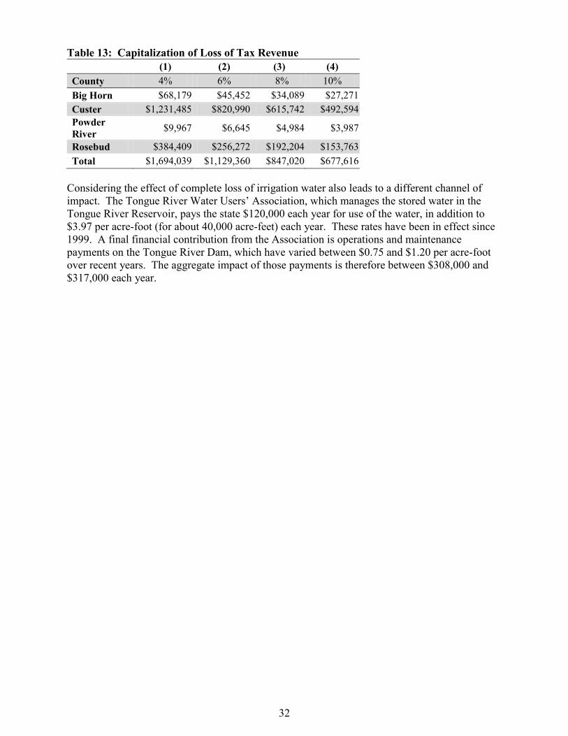
32
Table 13: Capitalization of Loss of Tax Revenue
(1) (2) (3) (4)
County 4% 6% 8% 10%
Big Horn $68,179 $45,452 $34,089 $27,271
Custer $1,231,485 $820,990 $615,742 $492,594
Powder
River $9,967 $6,645 $4,984 $3,987
Rosebud $384,409 $256,272 $192,204 $153,763
Total $1,694,039 $1,129,360 $847,020 $677,616
Considering the effect of complete loss of irrigation water also leads to a different channel of
impact. The Tongue River Water Users’ Association, which manages the stored water in the
Tongue River Reservoir, pays the state $120,000 each year for use of the water, in addition to
$3.97 per acre-foot (for about 40,000 acre-feet) each year. These rates have been in effect since
1999. A final financial contribution from the Association is operations and maintenance
payments on the Tongue River Dam, which have varied between $0.75 and $1.20 per acre-foot
over recent years. The aggregate impact of those payments is therefore between $308,000 and
$317,000 each year.
33
GENERAL DISCUSSION & CONCLUSIONS
This study estimates the agricultural production in the Montana portion of the Tongue River
watershed. Because water quality changes are specific to watersheds, the availability of
economic estimates pertaining to the spatial extent of expected effects improves the scope of
economic analysis. While the estimates focus on a handful of significant crops and the major
livestock output of the basin, they are likely representative of a broader spectrum of agricultural
activity.
Collectively, at most, the preliminary results assessing the impact of the Tongue River on
agricultural production provide weak support for a relationship between water availability and
aggregate agricultural production over time. The results for water quality are restricted by data
availability and do not indicate a strong pattern. This result may not be surprising given the low
correlation between diversions and water quality and quantity, at least for senior rights holders.
What is not clear at this point is whether this is because there are in fact not effects on production
from water quality, or whether the threshold that is needed to cause effects has not been reached,
or whether there has been adaptation on a finer time scale that we are not able to observe.
Consider the effect of poor water quality on growing crops. A farmer is likely to observe even
subtle signals and adjust input levels, including water application, in order to avoid economic
damages. The measures of agricultural production are annual, so farmers’ adjustments during
the growing season are masked. Learning about how to adapt over time (such as 30 years) is
also undetermined in this model. Certainly other agricultural inputs such as seed varieties and
irrigation technology have improved over the time examined, so it would be presumptuous to
assume that irrigators were not also learning and improving their human capital.
Montana has set aside revenues to compensate agricultural producers affected by the effluent
from CBM wells. While the results here are far from showing a causal link between CBM
outfalls and agricultural damages, the production and revenue figures offer a simple check on the
compensation fund. Individual farmers can claim up to $50,000 in damages, with an award
limited a 75 percent of total damage. Damages can be reduced land value or the losses from
reduced production. The 2007 Census of Agriculture estimated 325 farms in Montana that
harvest agricultural crops, which is an upper bound on the number of potential claims. If every
claimant received the maximum possible amount, the total could be $16.25 million. With the 75
percent of total damage provision, the aggregate damage could be $22 million. That figure is not
far from the annual gross revenue of agricultural production in the basin in 2010.
In conclusion, the study quantifies the importance of agriculture to the economy of southeastern
Montana. By estimating the primary agricultural production in the Tongue River Basin, this
study establishes a baseline for economic activity. Agricultural producers are involved in other
related enterprises that are not included in the estimates presented here, including protecting
wildlife habitat and furnishing outfitted recreational opportunities, breeding valuable horses, and
growing a variety of less widespread crops. Hence, in this respect, the estimates presented here
understate the importance of agriculture to the Tongue River economy
34
REFERENCES
ALL Consulting. 2003. Handbook on Coal Bed Methane Produced Water: Management and
Beneficial Use Alternatives. Prepared for: Ground Water Protection Research
Foundation; U.S. Dept. of Energy; National Petroleum Technology Office; Bureau of
Land Management. Tulsa, OK.
Barkey, Patrick and Paul E. Polzin. 2012. The Impact of Otter Creek Coal Development on the
Montana Economy. Bureau of Business & Economic Research, University of Montana.
Bauder, James. 2002. Quality and Characteristics of Saline and Sodic Water Affect Irrigation
Suitability. Montana State University Extension Water Quality Lab. Available at:
http://waterquality.montana.edu/docs/methane/irrigation_suitability.pdf
Boryan, Claire., Zhengwei Yang, Rick Mueller and Mike Craig. 2011. Monitoring US
Agriculture: The US Department of Agriculture Statistics Service, Cropland Data Layer
Program. Geocarto International. 26(5): 341-358.
Boysen, Deidre B., John E. Boysen, and Jessica A. Boysen. 2002. Strategic Produced Water
Management and Disposal Economics in the Rocky Mountain Region. BC Technologies,
Ltd.: Laramie, WY.
Cannon, M.R., David A. Nimick, Thomas E. Cleasby, Stacy M. Kinsey, and John H. Lambing.
2007. Measured and Estimated Sodium-Absorption Rations for Tongue River and its
Tributaries, Montana and Wyoming, 2004-06. USGS Scientific Investigations Report
2007-5072.
Clark, Melanie L. 2012. Water-quality characteristics and trend analyses for the Tongue,
Powder, Cheyenne, and Belle Fourche River drainage basins, Wyoming and Montana, for
selected periods, water years 1991 through 2010: U.S. Geological Survey Scientific
Investigations Report 2012–5117, pg. 70.
Clark, Melanie L., and Jon P. Mason. 2006. Water-Quality Characteristics, Including Sodium-
Adsorption Ratios, for Four Sites in the Powder River Drainage Basin, Wyoming and
Montana, Water Years 2001-2004: USGS Scientific Investigations Report 2006-5113.
Cropland Data Layer Frequently Anticipated Questions. Aug 1 2012.
http://www.nass.usda.gov/research/Cropland/sarsfaqs2.html
Dawson, Helen E. 2007. Pre- and Post-Coal Bed Natural Gas Development Surface Water
Quality Characteristics of Agricultural Concern in the Upper Tongue River Watershed
U.S. EPA, Region 8, Denver, CO.
Fitzgerald, Timothy. 2012. Prior Appropriation and Water Quality. Conservation Leadership
Council.
Ganjegunte, Girisha K., Lyle A. King., and George F. Vance. 2008. Cumulative Soil Chemistry
Changes from Land Application of Saline–Sodic Waters. Journal of Environmental
Quality. 37: S128- S138.
35
Kinsey, Stacy M. and David A. Nimick. 2011. Potential Water-Quality Effects of Coal-Bed
Methane Production Water Discharged along the Upper Tongue River, Wyoming and
Montana. Scientific Investigation Report 2011-5196. USGS: Reston, VA.
Kotuby-Amacher, Jan, Rich Koenig, Boyd Kitchen. 2000. Salinity and Plant Tolerance. Utah
State University Extension AG-SO-03
MacEwan, Duncan and Richard Howitt. 2012. Behavioral Salinity Response: Estimating
Salinity Policies from Remote Sensed Micro-Data. 56th
Annual AARES Conference
Paper, February, Freemantle, WA.
Myers, Tom. 2009. Groundwater management and coal bed methane development in the
Powder River Basin of Montana. Journal of Hydrology. 368: 178-193.
National Research Council. 2010. Management and Effects of Coalbed Methane Produced
Water in the United States. The National Academies Press.
Osborne, Thomas J., William M. Schafer, and Neal E. Fehringer. 2010. The agriculture-energy-
environment nexus in the West. Journal of Soil and Water Conservation. 65(3): 72A-
76A.
Schafer, William M. 1982. Saline and Sodic Soils in Montana. Extension Bulletin 1272.
Montana State University Cooperative Extension.
Stearns, M., J.A. Tindall, G. Cronin, M.J. Friedel, and E. Bergquist. 2005. Effects of coal-bed
methane discharge waters on the vegetation and soil ecosystem in Powder River Basin,
Wyoming. Water, Air, & Soil Pollution 168 (1): 33-57.
Suarez, D.L., J.D. Wood, and S.M. Lesch. 2006. Effect of SAR on water infiltration under a
sequential rain-irrigation management system, Agricultural Water Management, 86 (1):
150-164.
USDA. 2007 Census of Agriculture, Watersheds, Volume 2, Subject Series, Part 6.
Vance, G.F., G.K. Ganjegunte, and L.A. King. 2005. Soil chemical changes resulting from
irrigation with water co-produced with coalbed natural gas, Journal of Environmental
Quality, 34 (6): 2217-2227.
Warrence, Nikos J., and James W. Bauder. 2001. Salinity, Sodicity and Flooding Tolerance of
Selected Plant Species of the Northern Cheyenne Reservation. Montana State University
Extension Water Quality Program.
36
APPENDIX
DATA SOURCES AND METHODOLOGY
Method 1: Acreage Overlay
The first series was constructed using spatial statistics software to determine how many acres in
the four counties (Big Horn, Custer, Powder River, Rosebud) are in the Tongue watershed. See
table A1 for the weights. For each county, the ratio of its area in the watershed and its total area
was used as a weight for each individual county’s contribution to the watershed series. These
weights were applied to the corresponding county’s annual estimates for each year. As the
county and watershed boundaries are static, the weights do not change over time. This series
assumes that agricultural production is equally distributed across different watersheds, and
weights total county production by the fraction of acres in the TRB.
Method 2 & 3: Remote Sensing Overlay
The Cropland Data Layer (CDL) is a collection of Landsat satellite images using heat signatures
to estimate the acreage of different crops is produced on an annual basis.22
The data series is
available for Montana for years 2007-2011. One advantage of this remote sensing data is that
researchers are able to query each individual pixel within the image to determine the
predominant vegetation within that pixel. Early satellite imagery used for agriculture had a
resolution of 250 square meters (m2) per pixel, which, although enough to aid in estimating
changes in yields over time, is not detailed enough for field level data. The Landsat satellite
imagery used in the CDL has pixel resolutions of 30 square meters (m2). This more accurate data
can be used to estimate field-level crop content.5 Using the field-level estimates, a “bottom-up”
estimate of production within the TRB can be constructed. By comparing the remote-sensed
production within the TRB and remote-sensed production in the rest of the individual counties, a
different estimate of the TRB’s proportion of the county estimates is constructed. Since the CDL
data is annual, some of the variation in agricultural productivity over time can be incorporated
into the weighting algorithm.
The CDL provides data for nearly all crops produced, with over 100 different types of land cover
identified. Major land covers in the TRB are grassland, shrubland, and forestland. The major
crop types in all years are alfalfa hay, corn, and barley. Although this is a rich set of
information, the CDL data provides little information on crop yields and no information on what
was actually harvested.
Satellite imagery is subject to error. According to a report on the Cropland Data Layer, “Pixel
counting estimates…consistently underestimate the actual acreage number as compared with
NASS official estimates” (Boryan et al., 2011). NASS is able to correct for this underestimate
by regressing CDL data against ground collected data from the June Agricultural Survey (JAS)
and using the result to correct their produced CDL products for the rest of the year (Boryan et al.,
2011). Because geo-coded JAS data is not publicly available, it is not possible to replicate this.
Some crops, including alfalfa, have heat signatures that are similar to other types of vegetation.
NASS computers sometimes cannot distinguish between grass, hay, and alfalfa (Cropland Data
Layer FAQ). This problem was particularly pronounced in the 2008 data, but seems to have
been resolved in later years.
22
http://nassgeodata.gmu.edu/CropScape/
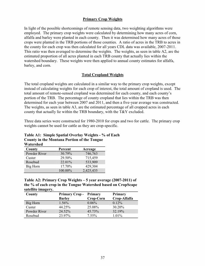
37
Primary Crop Weights
In light of the possible shortcomings of remote sensing data, two weighting algorithms were
employed. The primary crop weights were calculated by determining how many acres of corn,
alfalfa and barley were planted in each county. Then it was determined how many acres of those
crops were planted in the TRB portions of those counties. A ratio of acres in the TRB to acres in
the county for each crop was then calculated for all years CDL data was available, 2007-2011.
This ratio was then averaged to determine the weights. The weights, as seen in table A2, are the
estimated proportion of all acres planted in each TRB county that actually lies within the
watershed boundary. These weights were then applied to annual county estimates for alfalfa,
barley, and corn.
Total Cropland Weights
The total cropland weights are calculated in a similar way to the primary crop weights, except
instead of calculating weights for each crop of interest, the total amount of cropland is used. The
total amount of remote-sensed cropland was determined for each county, and each county’s
portion of the TRB. The percentage of county cropland that lies within the TRB was then
determined for each year between 2007 and 2011, and then a five-year average was constructed.
The weights, as seen in table A3, are the estimated percentage of all cropped acres in each
county that actually lie within the TRB boundary, with the T&Y excluded.
Three data series were constructed for 1980-2010 for crops and two for cattle. The primary crop
weights cannot be used for cattle as they are crop-specific.
Table A1: Simple Spatial Overlay Weights - % of Each
County in the Montana Portion of the Tongue
Watershed
County Percent Acreage
Powder River 30.79% 746,763
Custer 29.50% 715,459
Rosebud 22.01% 533,909
Big Horn 17.70% 429,304
100.00% 2,425,435
Table A2: Primary Crop Weights – 5 year average (2007-2011) of
the % of each crop in the Tongue Watershed based on CropScape
satellite imagery.
County Primary Crop -
Barley
Primary
Crop-Corn
Primary
Crop-Alfalfa
Big Horn 1.56% 0.06% 0.12%
Custer 44.25% 25.08% 30.20%
Powder River 24.52% 45.73% 32.19%
Rosebud 23.97% 7.55% 1.01%
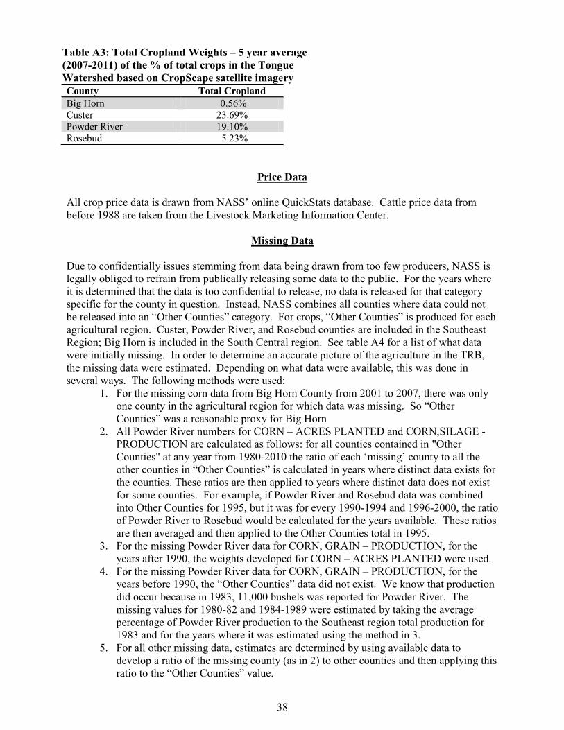
38
Table A3: Total Cropland Weights – 5 year average
(2007-2011) of the % of total crops in the Tongue
Watershed based on CropScape satellite imagery
County Total Cropland
Big Horn 0.56%
Custer 23.69%
Powder River 19.10%
Rosebud 5.23%
Price Data
All crop price data is drawn from NASS’ online QuickStats database. Cattle price data from
before 1988 are taken from the Livestock Marketing Information Center.
Missing Data
Due to confidentially issues stemming from data being drawn from too few producers, NASS is
legally obliged to refrain from publically releasing some data to the public. For the years where
it is determined that the data is too confidential to release, no data is released for that category
specific for the county in question. Instead, NASS combines all counties where data could not
be released into an “Other Counties” category. For crops, “Other Counties” is produced for each
agricultural region. Custer, Powder River, and Rosebud counties are included in the Southeast
Region; Big Horn is included in the South Central region. See table A4 for a list of what data
were initially missing. In order to determine an accurate picture of the agriculture in the TRB,
the missing data were estimated. Depending on what data were available, this was done in
several ways. The following methods were used:
1. For the missing corn data from Big Horn County from 2001 to 2007, there was only
one county in the agricultural region for which data was missing. So “Other
Counties” was a reasonable proxy for Big Horn
2. All Powder River numbers for CORN – ACRES PLANTED and CORN,SILAGE -
PRODUCTION are calculated as follows: for all counties contained in "Other
Counties" at any year from 1980-2010 the ratio of each ‘missing’ county to all the
other counties in “Other Counties” is calculated in years where distinct data exists for
the counties. These ratios are then applied to years where distinct data does not exist
for some counties. For example, if Powder River and Rosebud data was combined
into Other Counties for 1995, but it was for every 1990-1994 and 1996-2000, the ratio
of Powder River to Rosebud would be calculated for the years available. These ratios
are then averaged and then applied to the Other Counties total in 1995.
3. For the missing Powder River data for CORN, GRAIN – PRODUCTION, for the
years after 1990, the weights developed for CORN – ACRES PLANTED were used.
4. For the missing Powder River data for CORN, GRAIN – PRODUCTION, for the
years before 1990, the “Other Counties” data did not exist. We know that production
did occur because in 1983, 11,000 bushels was reported for Powder River. The
missing values for 1980-82 and 1984-1989 were estimated by taking the average
percentage of Powder River production to the Southeast region total production for
1983 and for the years where it was estimated using the method in 3.
5. For all other missing data, estimates are determined by using available data to
develop a ratio of the missing county (as in 2) to other counties and then applying this
ratio to the “Other Counties” value.

39
Estimation of these missing values increases the risk of error. While cognizant of this
possibility, of the methods used, those most likely to include error were used on corn data for
Powder River County. In comparison to the totals, these numbers are extremely low and thus
any error is extremely unlikely to significantly affect the final result. For the larger estimations,
the methods used were much more accurate and either did not increase the error at all, as was the
case with some data from Big Horn, or would only have increased it slightly.
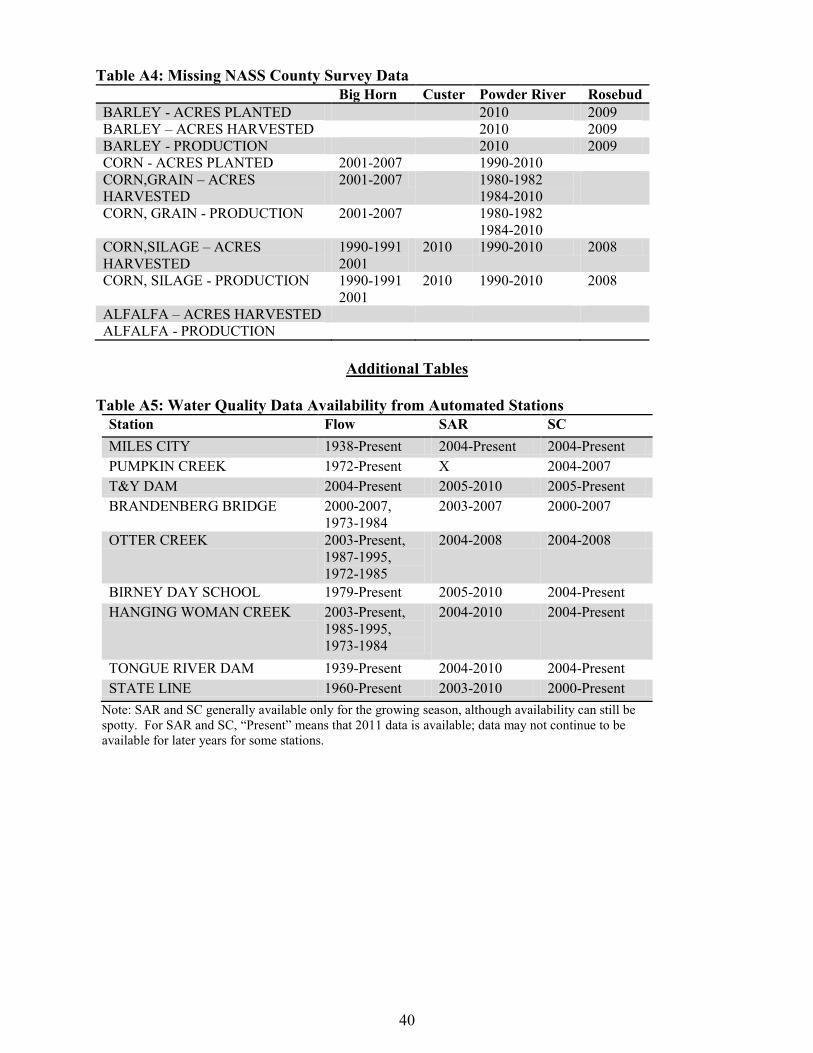
40
Table A4: Missing NASS County Survey Data
Big Horn Custer Powder River Rosebud
BARLEY - ACRES PLANTED 2010 2009
BARLEY – ACRES HARVESTED 2010 2009
BARLEY - PRODUCTION 2010 2009
CORN - ACRES PLANTED 2001-2007 1990-2010
CORN,GRAIN – ACRES
HARVESTED
2001-2007 1980-1982
1984-2010
CORN, GRAIN - PRODUCTION 2001-2007 1980-1982
1984-2010
CORN,SILAGE – ACRES
HARVESTED
1990-1991
2001
2010 1990-2010 2008
CORN, SILAGE - PRODUCTION 1990-1991
2001
2010 1990-2010 2008
ALFALFA – ACRES HARVESTED
ALFALFA - PRODUCTION
Additional Tables
Table A5: Water Quality Data Availability from Automated Stations
Station Flow SAR SC
MILES CITY 1938-Present 2004-Present 2004-Present
PUMPKIN CREEK 1972-Present X 2004-2007
T&Y DAM 2004-Present 2005-2010 2005-Present
BRANDENBERG BRIDGE 2000-2007,
1973-1984
2003-2007 2000-2007
OTTER CREEK 2003-Present,
1987-1995,
1972-1985
2004-2008 2004-2008
BIRNEY DAY SCHOOL 1979-Present 2005-2010 2004-Present
HANGING WOMAN CREEK 2003-Present,
1985-1995,
1973-1984
2004-2010 2004-Present
TONGUE RIVER DAM 1939-Present 2004-2010 2004-Present
STATE LINE 1960-Present 2003-2010 2000-Present
Note: SAR and SC generally available only for the growing season, although availability can still be
spotty. For SAR and SC, “Present” means that 2011 data is available; data may not continue to be
available for later years for some stations.
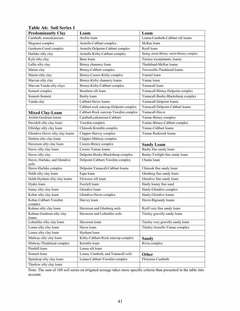
41
Table A6: Soil Series 1 Predominantly Clay Loam Loam Cambeth, noncalcareous- Archin loam Lonna-Cambeth-Cabbart silt loams
Megonot complex Armells-Cabbart complex McRae loam
Gerdrum-Creed complex Armells-Delpoint-Cabbart complex Ryell loam
Harlake silty clay Armells-Kirby-Cabbart complex Spang, moist-Birney, moist-Birney complex
Kyle silty clay Benz loam Terrace escarpments, loamy
Lallie silty clay Birney channery loam Thedalund-McRae loams
Marias clay Birney-Cabbart complex Travessilla-Thedalund loams
Marias silty clay Birney-Cooers-Kirby complex Vanstel loam
Marvan silty clay Birney-Kirby channery loams Yamac loam
Marvan-Vanda silty clays Birney-Kirby-Cabbart complex Yamacall loam
Sonnett complex Brushton silt loam Yamacall-Birney-Delpoint complex
Sonnett-Sonnett Busby loam Yamacall-Busby-Blacksheep complex
Vanda clay Cabbart-Havre loams Yamacall-Delpoint loams
Cabbart-rock outcrop-Delpoint complex Yamacall-Delpoint-Cabbart loams
Mixed Clay-Loam Cabbart-Rock outcrop-Yawdim complex Yamacall-Havre
Archin-Gerdrum loams Cambeth,calcareous-Cabbart- Yamac-Birney complex
Davidell silty clay loam Yawdim complex Yamac-Birney-Cabbart complex
Ethridge silty clay loam Chinook-Kremlin complex Yamac-Cabbart loams
Glendive-Havre silty clay loams Clapper-Harvey complex Yamac-Redcreek loams
Harlem silty clay loam Clapper-Midway complex Haverson silty clay loam Cooers-Birney complex Sandy Loam Havre silty clay loam Cooers-Yamac loams Busby fine sandy loam
Havre silty clay Delpoint-Busby-Blacksheep complex Busby-Twilight fine sandy loam
Havre, Harlake, and Glendive
soils
Delpoint-Cabbart-Yawdim complex Chanta loam
Havre-Harlake complex Delpoint-Yamacall-Cabbart loams Chinook fine sandy loam
Heldt silty clay loam Eapa loam Glenberg fine sandy loam
Heldt-Hysham silty clay loams Floweree silt loam Glendive fine sandy loam
Hydro loam Foreleft loam Hanly loamy fine sand
Ismay silty clay loam Glendive loam Hanly-Glendive complex
Kobar silty clay loam Glendive-Havre complex Hanly-Glendive loams
Kobar-Cabbart-Yawdim
complex
Harvey loam Havre-Bigsandy loams
Kobase silty clay loam Haverson and Glenberg soils Ryell very fine sandy loam
Kobase-Gerdrum silty clay
loams
Haverson and Lohmiller soils Tinsley gravelly sandy loam
Lohmiller silty clay loam Haverson loam Tinsley very gravelly sandy loam
Lonna silty clay loam Havre loam Tinsley-Armells-Yamac complex
Lonna silty clay loam Hysham loam Midway silty clay loam Kirby-Cabbart-Rock outcrop complex Sandy Midway-Thedalund complex Kremlin loam Rivra complex
Pinehill loam Lonna silt loam Sonnett loam Lonna, Cambeth, and Yamacall soils Other Spinekop silty clay loam Lonna-Cabbart-Yawdim complex Floweree-Cambeth
Thurlow silty clay loam Note: The sum of 160 soil series on irrigated acreage takes more specific criteria than presented in the table into
account.

42
Copyright 2013 All rights reserved.
The U.S. Department of Agriculture (USDA), Montana State University and the Montana State University Extension
prohibit discrimination in all of their programs and activities on the basis of race, color, national origin, gender, religion,
age, disability, political beliefs, sexual orientation, and marital and family status. Issued in furtherance of cooperative
extension work in agriculture and home economics, acts of May 8 and June 30, 1914, in cooperation with the U.S.
Department of Agriculture, Jill Martz, Interim Director of Extension, Montana State University, Bozeman, MT 59717.