agilent technologies 1670g series logic analyzers · agilent technologies 1670g-series logic...
TRANSCRIPT
User’s Guide
Publication Number 01670-97022August 2002
For Safety information, Warranties, and Regulatory information, see the pages behind the index.
© Copyright Agilent Technologies 1994-2002All Rights Reserved
Agilent Technologies 1670G Series Logic Analyzers
Agilent Technologies 1670G-Series Logic Analyzers
The Agilent Technologies 1670G-Series is a 150-MHz State/500-MHz Timing Logic Analyzer with a VGA resolution color display. The 1670G-Series logic analyzer has two options available. One option is to add a 2 GSa/s digitizing oscilloscope. Another option is to add a 32 channel pattern generator.
Logic Analyzer Features
• 130 data channels and 6 clock/data channels in the 1670G
• 96 data channels and 6 clock/data channels in the 1671G
• 64 data channels and 4 clock/data channels in the 1672G
• 32 data channels and 2 clock/data channels in the 1673G
• 3.5-inch flexible disk drive
• 2 GB hard disk drive
• GPIB, RS-232-C, parallel printer, and LAN interfaces
• BNC and TP LAN ports
• Variable setup/hold time
• 64k memory on all channels with 256k and 2M options
• Marker measurements
• 12 levels of trigger sequencing for state and 10 levels of trigger sequencing for timing
• Time tagging and number-of-states tagging
• Full programmability
• DIN mouse and keyboard support
2
Oscilloscope Features (Option)
• 500 MHz bandwidth
• 2 Gigasample per second max sampling rate
• >32000 samples per channel
• Marker measurementsdisplays time between markers, acquires until specified time between markers in captured, performs statistical analysis on time between markers
• Lightweight miniprobes
Pattern Generator Features (Option)
• 16 output channels at 200 MHz
• 32 output channels at 100 MHz
• 258,048 vectors
Documentation Options
• Programmer's Guide
• Service Guide
• Training Kit
3

In This Book
This User’s Guide has three sections. Section 1 covers how to use the 1670G-series logic analyzers. Section 2 covers how to connect, use, and troubleshoot the logic analyzer via a Local Area Network (LAN) connection. Section 3 covers the features of the Agilent Technologies Symbol Utility software.
Section 1. Chapters 1 through 4 cover general product information you need to use the logic analyzer. Chapter 5 and 6 contains detailed examples to help you use your analyzer in performing complex measurements. Chapter 7 covers how to use the oscilloscope (Option). Chapter 8 covers how to use the pattern generator (Option). Chapters 9 through 11 contains reference information on the hardware and software, including the analyzer menus and how they are used. Chapters 12 through 14 provides a basic service guide.
Section 2. Chapters 15 through 16 provides information about connecting the logic analyzer to the network. Chapter 17 shows you how to access the logic analyzer’s file system. Chapter 18 shows you how to display the analyzer interface on an X Window server. Chapter 19 shows you how to retrieve measurement data, screen images, and status information from you logic analyzer on the LAN, and how to copy and restore configurations. Chapter 20 shows you methods for programming the logic analyzer via the network connection. Chapter 21 contains additional information on the logic analyzer’s directory structure and dynamic files. Chapter 22 describes what to do if you have a problem using the logic analyzer on your network.
Section 3. Chapters 23 through 24 describe how to locate the menus associated with the Symbol Utility. Chapter 25 describes how to use the Symbol Utility to perform common tasks. Chapter 26 describes the features and functions of the Symbol Utility.
4

Contents
Agilent Technologies 1670G-Series Logic Analyzers
In This Book
1 Logic Analyzer Overview
Agilent Technologies 1670G-Series Logic Analyzer 26To make a measurement 29
2 Connecting Peripherals
Connecting Peripherals 36To connect a mouse 37To connect a keyboard 38To connect to an GPIB printer 39To connect to an RS-232-C printer 41To connect to a parallel printer 43To connect to a controller 44
3 Using the Logic Analyzer
Using the Logic Analyzer 46
Accessing the Menus 47To access the System menus 48To access the Analyzer menus 50
5
Contents
Using the Analyzer Menus 52To label channel groups 52To create a symbol 55To examine an analyzer waveform 57To examine an analyzer listing 60To compare two listings 63
The Inverse Assembler 65To use an inverse assembler 65
4 Using the Trigger Menu
Using the Trigger Menu 70
Specifying a Basic Trigger 71To assign terms to an analyzer 72To define a term 74To change the trigger specification 75
Changing the Trigger Sequence 77To add sequence levels 78To change trigger functions 80
Setting Up Time Correlation between Analyzers 81To set up time correlation between two state analyzers 82To set up time correlation between a timing and a state analyzer 83
Arming and Additional Instruments 84To arm another instrument 84To arm the oscilloscope with the analyzer (1670G-series logic analyzers with the oscilloscope option) 85To receive an arm signal from another instrument 87
6

Contents
Managing Memory 89To selectively store branch conditions (state only) 90To set the memory length 91To place the trigger in memory 93To set the sampling rates (Timing only) 94
5 Triggering Examples
Triggering Examples 96
Single-Machine Trigger Examples 97To store and time the execution of a subroutine 98To trigger on the nth iteration of a loop 100To trigger on the nth recursive call of a recursive function 102To trigger on entry to a function 104To capture a write of known bad data to a particular variable 106To trigger on a loop that occasionally runs too long 107To verify correct return from a function call 108To trigger after all status bus lines finish transitioning 109To find the nth assertion of a chip select line 110To verify that the chip select line is strobed after the address is stable 111To trigger when expected data does not appear when requested 112To test minimum and maximum pulse limits 114To detect a handshake violation 116To detect bus contention 117
Cross-Arming Trigger Examples 118To examine software execution when a timing violation occurs 119To look at control and status signals during execution of a routine 121To detect a glitch 122To capture the waveform of a glitch using the oscilloscope (oscilloscope option only) 123To view your target system processing an interrupt (oscilloscope option
7
Contents
only) 124To trigger timing analysis of a count-down on a set of data lines 125To monitor two coprocessors in a target system 126
Special Displays 128To interleave trace lists 129To view trace lists and waveforms on the same display 131
6 File Management
File Management 134
Transferring Files Using the Flexible Disk Drive 135To save a configuration 136To load a configuration 137To save a trace list in ASCII format 139To save a screen's image 140To load additional software 141
Transferring Files Using the LAN 142To transfer files using ftp 143
7 Using the Oscilloscope
Using the Oscilloscope 146
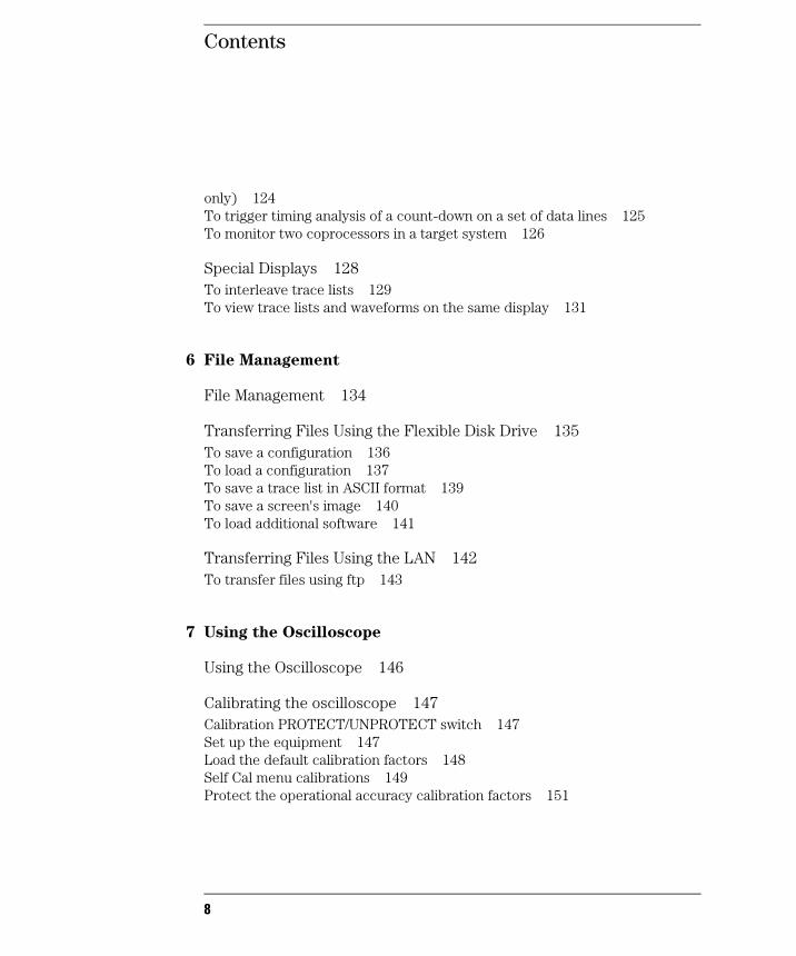
Calibrating the oscilloscope 147Calibration PROTECT/UNPROTECT switch 147Set up the equipment 147Load the default calibration factors 148Self Cal menu calibrations 149Protect the operational accuracy calibration factors 151
8
Contents
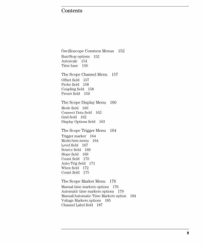
Oscilloscope Common Menus 152Run/Stop options 152Autoscale 154Time base 156
The Scope Channel Menu 157Offset field 157Probe field 158Coupling field 158Preset field 159
The Scope Display Menu 160Mode field 160Connect Dots field 162Grid field 162Display Options field 163
The Scope Trigger Menu 164Trigger marker 164Mode/Arm menu 164Level field 167Source field 169Slope field 169Count field 170Auto-Trig field 171When field 172Count field 175
The Scope Marker Menu 176Manual time markers options 176Automatic time markers options 179Manual/Automatic Time Markers option 184Voltage Markers options 185Channel Label field 187
9

Contents
The Scope Auto Measure Menu 188Input field 188Automatic measurements display 189Automatic measurement algorithms 191
8 Using the Pattern Generator
Using the Pattern Generator 196
Setting Up the Proper Configurations 197To set up the configuration 197To build a label 199
Building Test Vectors and Functions 200To build a main vector sequence 201To build an initialization sequence 202To edit a main or initialization sequence 203To include hardware instructions in a sequence 204To include software instructions in a sequence 205To include a user macro in a sequence 206To build a user macro 207To modify a function name 208To edit a function 208To add, delete, or rename parameters 209To place parameters in a vector 210To enter or modify parameters 211To build a User Symbol Table 212To include symbols in a sequence 213To include symbols in a function 214To store a configuration 215To load a configuration 216To use Autoroll 217The Format Menu 218The Sequence Menu 222The User Macros Menu 231
10
Contents
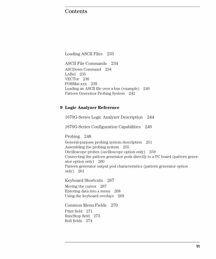
Loading ASCII Files 233
ASCII File Commands 234ASCDown Command 234LABel 235VECTor 236FORMat:xxx 239Loading an ASCII file over a bus (example) 240Pattern Generator Probing System 242
9 Logic Analyzer Reference
1670G-Series Logic Analyzer Description 244
1670G-Series Configuration Capabilities 246
Probing 248General-purpose probing system description 251Assembling the probing system 255Oscilloscope probes (oscilloscope option only) 259Connecting the pattern generator pods directly to a PC board (pattern gener-ator option only) 260Pattern generator output pod characteristics (pattern generator option only) 261
Keyboard Shortcuts 267Moving the cursor 267Entering data into a menu 268Using the keyboard overlays 269
Common Menu Fields 270Print field 271Run/Stop field 273Roll fields 274
11
Contents
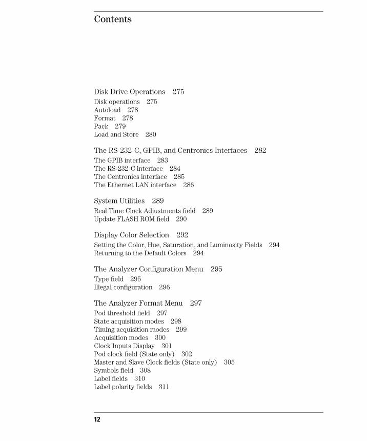
Disk Drive Operations 275Disk operations 275Autoload 278Format 278Pack 279Load and Store 280
The RS-232-C, GPIB, and Centronics Interfaces 282The GPIB interface 283The RS-232-C interface 284The Centronics interface 285The Ethernet LAN interface 286
System Utilities 289Real Time Clock Adjustments field 289Update FLASH ROM field 290
Display Color Selection 292Setting the Color, Hue, Saturation, and Luminosity Fields 294Returning to the Default Colors 294
The Analyzer Configuration Menu 295Type field 295Illegal configuration 296
The Analyzer Format Menu 297Pod threshold field 297State acquisition modes 298Timing acquisition modes 299Acquisition modes 300Clock Inputs Display 301Pod clock field (State only) 302Master and Slave Clock fields (State only) 305Symbols field 308Label fields 310Label polarity fields 311
12
Contents
The Analyzer Trigger Menu 312Trigger sequence levels 312Modify Trigger field 313Timing trigger function library 314State trigger function library 316Modifying the user function 319Resource terms 323Arming Control field 327Acquisition Control field 329Count field (State only) 331
The Listing Menu 332Markers 332
The Waveform Menu 334sec/Div field 334Accumulate field 334Delay field 335Waveform label field 335Waveform display 337
The Mixed Display Menu 338Interleaving state listings 338Time-correlated displays 339Markers 339
The Chart Menu 340Min and Max scaling fields 341Markers/Range field 341Axis Control field 342Rescale field 343
13
Contents
The Compare Menu 344Reference Listing field 345Difference Listing field 345Copy Listing to Reference field 346Find Error field 347Compare Full/Compare Partial field 347
10 System Performance Analysis (SPA) Software
System Performance Analysis Software 350What is System Performance Analysis? 352Getting started 355SPA measurement processes 357Using State Overview, State Histogram, and Time Interval 373Using SPA with other features 383
11 Logic Analyzer Concepts
Logic Analyzer Concepts 386
The File System 387Directories 388File types 389
The Trigger Sequence 391Trigger sequence specification 392Analyzer resources 395Timing analyzer 400State analyzer 400
Configuration Translation Between Agilent Logic Analyzers 401
14
Contents
The Analyzer Hardware 4031670G-series analyzer theory 404Logic acquisition board theory 408Oscilloscope board theory 412Pattern Generator board theory 417Self-tests description 420
12 Troubleshooting the Logic Analyzer
Troubleshooting the Logic Analyzer 422
Analyzer Problems 423Intermittent data errors 423Unwanted triggers 424No activity on activity indicators 424Capacitive loading 425No trace list display 425
Analysis Probe Problems 426Target system will not boot up 426Slow clock 427Erratic trace measurements 428
Inverse Assembler Problems 429No inverse assembly or incorrect inverse assembly 429Inverse assembler will not load or run 431
15

Contents
Error Messages 432". . . Inverse Assembler Not Found" 432"No Configuration File Loaded" 432"Selected File is Incompatible" 433"Slow or Missing Clock" 433"Waiting for Trigger" 433"Must have at least 1 edge specified" 434"Time correlation of data is not possible" 434"Maximum of 32 channels per label" 434"Timer is off in sequence level n where it is used" 435"Timer is specified in sequence, but never started" 435"Inverse assembler not loaded - bad object code." 435"Measurement Initialization Error" 436"Warning: Run HALTED due to variable change" 436
13 Specifications
General Information 438Accessories 438Specifications (logic analyzer) 440Specifications (oscilloscope option) 441Characteristics (logic analyzer) 442Characteristics (oscilloscope) 443Characteristics (pattern generator) 443Supplemental characteristics (logic analyzer) 445Supplemental characteristics (oscilloscope) 450Operating environment 452
14 Operator’s Service
Operator’s Service 454
16
Contents
Preparing For Use 455To inspect the logic analyzer 456To apply power 456To clean the logic analyzer 457To test the logic analyzer 457
Troubleshooting 458To use the flowcharts 459To check the power-up tests 461To run the self-tests 462To test the auxiliary power 471
15 Introducing the LAN Interface
Introducing the LAN Interface 476LAN section overview 478
16 Connecting and Configuring the LAN
Connecting and Configuring the LAN 480To connect to your network 481To configure the network addresses 482To verify connectivity with the ping utility 485To mount the logic analyzer 486
17 Accessing the Logic Analyzer File System Using the LAN
Accessing the Logic Analyzer File System Using the LAN 490Control User vs. Data User 490To mount the file system via NFS 491To access the file system via ftp 496
17
Contents
18 Using the LAN’s X Window Interface
Using the LAN’s X Window Interface 498To start the interface from the front panel 499To start the interface from the computer 501To close the interface 504To load the custom fonts 505Additional Information 508
19 Retrieving and Restoring Data Using the LAN
Retrieving and Restoring Data Using the LAN 510To copy ASCII measurement data 511To copy raw measurement data 512To restore raw measurement data 513To copy screen images from \system\graphics 514To copy status information from \status 515To copy configurations from setup.raw 517To restore configurations 518
20 Programming the Logic Analyzer Using the LAN
Programming the Logic Analyzer Using the LAN 520To set up for Ethernet LAN programming 521To enter commands directly using telnet 522To write programs that open the command parser socket 524
21 LAN Concepts
LAN Concepts 528Directory structure of the logic analyzer's file system 529Dynamic files 532LAN-related fields in the logic analyzer's menus 533
18
Contents
22 Troubleshooting the LAN Connection
Troubleshooting the LAN Connection 536
Troubleshooting the Initial Connection 537Assess the problem 537Troubleshooting in a workstation environment 540Troubleshooting in an MS-DOS environment 542Troubleshooting in an MS Windows environment 544Verify the logic analyzer performance 546Status Number 548Network Status Information 551
Solutions to Common Problems 553If you cannot connect to the logic analyzer 553If you cannot mount the logic analyzer file system 554If you cannot access the file system via ftp 554If you cannot start the XWindow interface 555If your X Window looks odd 555If you cannot copy files from the logic analyzer 556If you cannot restore raw files 556If you get an "operation timed-out" message 557If the logic analyzer begins to operate slowly 557If the logic analyzer does not respond 557If all else fails 558
Getting Service Support 559Return to Agilent service 559
23 Symbol Utility Introduction
Symbol Utility Introduction 564Equipment Required 564Supported Symbol File Formats 565Symbol Utility section overview 567
19
Contents
24 Getting Started with the Symbol Utility
Getting Started with the Symbol Utility 570To Access the Symbol File Load Menu 571Method 1: Using the Module Field 571Method 2: Using the Symbol Field in the Format Menu 573To Access the Symbol Browser 575
25 Using the Symbol Utility
To generate a symbol file 578To Load a Symbol File 579To Display Symbols in the Trace List 582To Trigger on a Symbol 583To View a List of Symbol Files Currently Loaded into the System 585To Remove a Symbol File From the System 586
26 Symbol Utility Features and Functions
Symbol Utility Features and Functions 588
The OMF Symbol File Load Menu 589OMF File Field 590Drive Field 590Label Field 591Module Field 591Load Field 592Current Loaded Files Field 593Section Relocation Option 594
20
Contents
The OMF Symbol Browser Menu 596Symbol Type Selection Field (User vs. OMF) 597Find Field 598Browse Results Display 600Align to xx Byte Option 601Offset Option 602Context Display 603Address Display 603Symbol Mode Field 604
The General-Purpose ASCII File Format 605Creating a GPA Symbol File 606GPA File Format 607Sections 609Functions 611Variables 612Source Line Numbers 613Start Address 614Comments 614
21

Contents
22
Section 1
Logic Analyzer
23

24
1
Logic Analyzer Overview
25
Logic Analyzer OverviewAgilent Technologies 1670G-Series Logic Analyzer
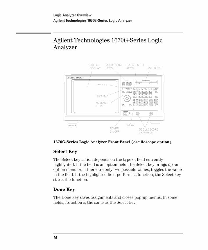
Agilent Technologies 1670G-Series Logic Analyzer
1670G-Series Logic Analyzer Front Panel (oscilloscope option)
Select Key
The Select key action depends on the type of field currently highlighted. If the field is an option field, the Select key brings up an option menu or, if there are only two possible values, toggles the value in the field. If the highlighted field performs a function, the Select key starts the function.
Done Key
The Done key saves assignments and closes pop-up menus. In some fields, its action is the same as the Select key.
26
Logic Analyzer OverviewAgilent Technologies 1670G-Series Logic Analyzer
Shift Key
The Shift key, which is blue, provides lowercase letters and access to the functions in blue on some of the keys. You do not need to hold the shift key down while pressing the other key. Press the shift key first, and then the function key.
Knob
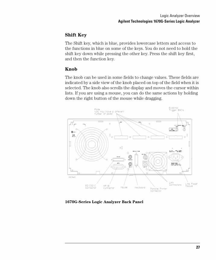
The knob can be used in some fields to change values. These fields are indicated by a side view of the knob placed on top of the field when it is selected. The knob also scrolls the display and moves the cursor within lists. If you are using a mouse, you can do the same actions by holding down the right button of the mouse while dragging.
1670G-Series Logic Analyzer Back Panel
27
Logic Analyzer OverviewAgilent Technologies 1670G-Series Logic Analyzer
External Trigger BNCs
The External Trigger BNCs provide the "Port In" and "Port Out" connections for the Arm In and Arm Out of the Trigger Arming Control menu.
RS-232-C Connector
Standard DB-25 type connector for connecting an RS-232-C printer or controller.
GPIB Connector
Standard GPIB connector for connecting an GPIB printer or controller.
Parallel Printer Connector
Standard Centronics connector for connecting a parallel printer.
LAN Connectors
Connects the logic analyzer to your local ethernet network. The BNC connector on top accepts 10Base2 ("thinlan"). The UTP connector below the BNC connector accepts 10Base-T ("ethertwist").
Calibration Memory Switch
Provides write protection for the calibration factors stored in memory.
Active Probe Power
Provides the power needed for active probes such as the Agilent Technologies 1144A.
28

Logic Analyzer OverviewAgilent Technologies 1670G-Series Logic Analyzer
To make a measurement
For more detail on any of the information below, see the referenced chapters or the Logic Analyzer Training Kit. If you are using an analysis probe with the logic analyzer, some of these steps may not apply.
Map to target
Connect probes
Connect probes from the target system to the logic analyzer to physically map the target system to the channels in the logic analyzer. Attach probes to a pod in a way that keeps logically-related channels together. Remember to ground the pod.
See Also "Probing" on page 248 for more detail on constructing probes.
Set type
When the logic analyzer is turned on, Analyzer 1 is named Machine 1 and is configured as a timing analyzer, and Analyzer 2 is off. To use state analysis or software profiling, you must set the type of the analyzer in the Analyzer Configuration menu. You can only use one timing analyzer at a time.
29

Logic Analyzer OverviewAgilent Technologies 1670G-Series Logic Analyzer
Assign pods
In the Analyzer Configuration menu, assign the connected pods to the analyzer you want to use. The number of pods on your logic analyzer depends on the model. Pods are paired and always assigned as a pair to a particular analyzer.
Set up analyzers
Set modes and clocks
Set the state and timing analyzers using the Analyzer Format menu. In general, these modes trade channel count for speed or storage. The state analyzer also provides for complicated clocking. If your state clock is set incorrectly, the data gathered by the logic analyzer might indicate an error where none exists.
See Also "The Analyzer Format Menu" on page 297 for more information on modes and clocks.
Group bits under labels
The Analyzer Format menu indicates active pod bits. You can create groups of bits across pods or subgroups within pods and name the groups or subgroups using labels.
30
Logic Analyzer OverviewAgilent Technologies 1670G-Series Logic Analyzer
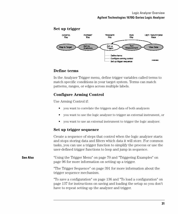
Set up trigger
Define terms
In the Analyzer Trigger menu, define trigger variables called terms to match specific conditions in your target system. Terms can match patterns, ranges, or edges across multiple labels.
Configure Arming Control
Use Arming Control if:
• you want to correlate the triggers and data of both analyzers
• you want to use the logic analyzer to trigger an external instrument, or
• you want to use an external instrument to trigger the logic analyzer.
Set up trigger sequence
Create a sequence of steps that control when the logic analyzer starts and stops storing data and filters which data it will store. For common tasks, you can use a trigger function to simplify the process or use the user-defined trigger functions to loop and jump in sequence.
See Also "Using the Trigger Menu" on page 70 and "Triggering Examples" on page 96 for more information on setting up a trigger.
"The Trigger Sequence" on page 391 for more information about the trigger sequence mechanism.
"To save a configuration" on page 136 and "To load a configuration" on page 137 for instructions on saving and loading the setup so you don't have to repeat setting up the analyzer and trigger.
31
Logic Analyzer OverviewAgilent Technologies 1670G-Series Logic Analyzer
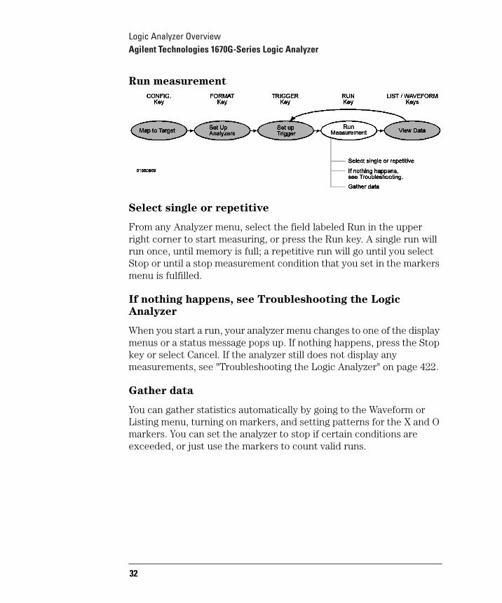
Run measurement
Select single or repetitive
From any Analyzer menu, select the field labeled Run in the upper right corner to start measuring, or press the Run key. A single run will run once, until memory is full; a repetitive run will go until you select Stop or until a stop measurement condition that you set in the markers menu is fulfilled.
If nothing happens, see Troubleshooting the Logic
Analyzer
When you start a run, your analyzer menu changes to one of the display menus or a status message pops up. If nothing happens, press the Stop key or select Cancel. If the analyzer still does not display any measurements, see "Troubleshooting the Logic Analyzer" on page 422.
Gather data
You can gather statistics automatically by going to the Waveform or Listing menu, turning on markers, and setting patterns for the X and O markers. You can set the analyzer to stop if certain conditions are exceeded, or just use the markers to count valid runs.
32
Logic Analyzer OverviewAgilent Technologies 1670G-Series Logic Analyzer
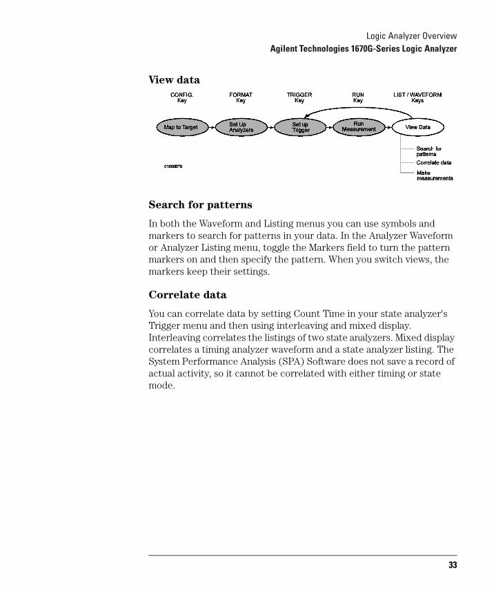
View data
Search for patterns
In both the Waveform and Listing menus you can use symbols and markers to search for patterns in your data. In the Analyzer Waveform or Analyzer Listing menu, toggle the Markers field to turn the pattern markers on and then specify the pattern. When you switch views, the markers keep their settings.
Correlate data
You can correlate data by setting Count Time in your state analyzer's Trigger menu and then using interleaving and mixed display. Interleaving correlates the listings of two state analyzers. Mixed display correlates a timing analyzer waveform and a state analyzer listing. The System Performance Analysis (SPA) Software does not save a record of actual activity, so it cannot be correlated with either timing or state mode.
33
Logic Analyzer OverviewAgilent Technologies 1670G-Series Logic Analyzer
Make measurements
The markers can count occurrences of events, measure durations, and collect statistics, and SPA provides high-level summaries to help you identify bottlenecks. To use the markers, select the appropriate marker type in the display menu and specify the data patterns for the marker. To use SPA, go to the SPA menu, select the most appropriate mode, fill in the parameters, and press Run.
See Also "System Performance Analysis (SPA) Software" on page 350 for more information on using SPA.
"The Waveform Menu" on page 334 and "The Listing Menu" on page 332 for additional information on the menu features.
34
2
Connecting Peripherals
35
Connecting PeripheralsConnecting Peripherals
Connecting PeripheralsThe 1670G-series logic analyzers comes with a PS2 mouse. It also provides connectors for a keyboard, Centronics (parallel) printer, and GPIB and RS-232-C devices. This chapter tells you how to connect peripheral equipment such as the mouse or a printer to the logic analyzer.
Mouse and Keyboard
You can use either the supplied mouse and optional keyboard, or another PS2 mouse and keyboard with standard DIN connector. The DIN connector is the type commonly used by personal computer accessories.
Printers
The logic analyzer communicates directly with HP PCL printers supporting the printer control language or with other printers supporting the Epson standard command set. Many non-Epson printers have an Epson-emulation mode. HP PCL printers include the following:
• HP ThinkJet
• HP LaserJet
• HP PaintJet
• HP DeskJet
• HP QuietJet
You can connect your printer to the logic analyzer using GPIB, RS-232-C, or the parallel printer port. The logic analyzer can only print to printers directly connected to it. It cannot print to a networked printer.
36

Connecting PeripheralsConnecting Peripherals
To connect a mouse
Agilent Technologies supplies a mouse with the logic analyzer. If you prefer a different style of mouse you can use any PS2 mouse with a standard PS2 DIN interface.
1 Plug the mouse into the mouse connector on the back panel. Make sure the plug shows the arrow on top.
2 To verify connection, check the System External I/O menu for a mouse box.
The mouse box is on the right side above the Settings fields. If the logic analyzer was displaying the System External I/O menu when you plugged in the mouse, the menu won't update until you exit and then return to it.
The mouse pointer looks like a plus sign (+). To select a field, move the pointer over it and press the left button. To duplicate the front-panel knob, hold down the right button while moving the mouse. Moving the mouse up or to the right duplicates turning the knob clockwise. Moving the mouse down or to the left duplicates turning the knob counterclockwise.
System External I/O Menu Showing Mouse Installed
37
Connecting PeripheralsConnecting Peripherals
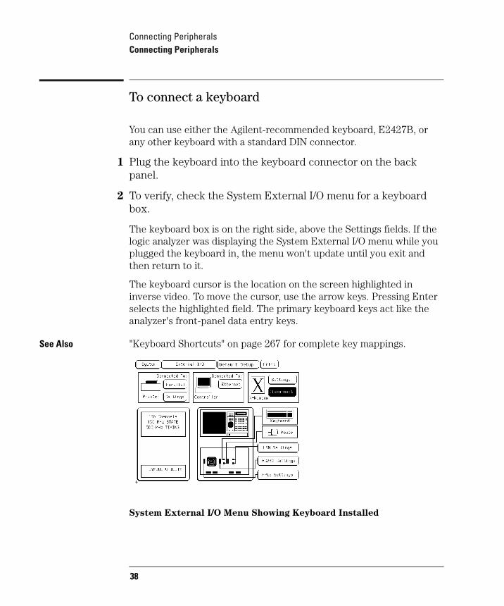
To connect a keyboard
You can use either the Agilent-recommended keyboard, E2427B, or any other keyboard with a standard DIN connector.
1 Plug the keyboard into the keyboard connector on the back panel.
2 To verify, check the System External I/O menu for a keyboard box.
The keyboard box is on the right side, above the Settings fields. If the logic analyzer was displaying the System External I/O menu while you plugged the keyboard in, the menu won't update until you exit and then return to it.
The keyboard cursor is the location on the screen highlighted in inverse video. To move the cursor, use the arrow keys. Pressing Enter selects the highlighted field. The primary keyboard keys act like the analyzer's front-panel data entry keys.
See Also "Keyboard Shortcuts" on page 267 for complete key mappings.
System External I/O Menu Showing Keyboard Installed
38
Connecting PeripheralsConnecting Peripherals
To connect to an GPIB printer
Printers connected to the logic analyzer over GPIB must support GPIB and Listen Always. When controlling a printer, the analyzer's GPIB port does not respond to service requests (SRQ), so the SRQ enable setting does not have any effect on printer operation.
1 Turn off the analyzer and the printer, and connect an GPIB cable from the printer to the GPIB connector on the analyzer rear panel.
2 Turn on the analyzer and printer.
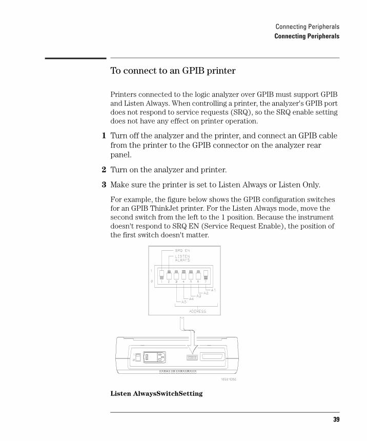
3 Make sure the printer is set to Listen Always or Listen Only.
For example, the figure below shows the GPIB configuration switches for an GPIB ThinkJet printer. For the Listen Always mode, move the second switch from the left to the 1 position. Because the instrument doesn't respond to SRQ EN (Service Request Enable), the position of the first switch doesn't matter.
Listen AlwaysSwitchSetting
39
Connecting PeripheralsConnecting Peripherals
4 Go to the System External I/O menu and configure the analyzer's printer settings.
a If the analyzer is not already set to GPIB, select the field under Connected To: in the Printer box and choose GPIB from the menu.
b Select the Printer Settings field.
c In the top field of the pop-up, select the type of printer you are using. If you are using an Epson graphics printer or an Epson-compatible printer, select Alternate.
d If the default print width and page length are not what you want, select the fields to toggle them.If you select 132 characters per line when using a printer other than QuietJet, the listings are printed in a compressed mode. QuietJet printers can print 132 characters per line without going to compressed mode, but require wider paper.
e Press Done.
40
Connecting PeripheralsConnecting Peripherals
To connect to an RS-232-C printer
1 Turn off the analyzer and the printer, and connect a null-modem RS-232-C cable from the printer to the RS-232-C connector on the analyzer rear panel.
2 Before turning on the printer, locate the mode configuration switches on the printer and set them as follows:
• For the HP QuietJet series printers, there are two banks of mode function switches inside the front cover. Push all the switches down to the 0 position.
• For the HP ThinkJet printer, the mode switches are on the rear panel of the printer. Push all the switches down to the 0 position.
• For the HP LaserJet printer, the factory default switch settings are okay.
3 Turn on the analyzer and printer.
4 Go to the System External I/O menu and configure the analyzer's printer settings.
a If the analyzer is not already set to RS232, select the field under Connected To: in the Printer box and choose RS232 from the menu.
b Select the Printer Settings field.
c In the top field of the pop-up, select the type of printer you are using. If you are using an Epson graphics printer or an Epson-compatible printer, select Alternate.
41
Connecting PeripheralsConnecting Peripherals
d If the default print width and page length are not what you want, select the fields to toggle them.If you select 132 characters per line when using a printer other than QuietJet, the listings are printed in a compressed mode. QuietJet printers can print 132 characters per line without going to compressed mode, but require wider paper.
e Press Done.
5 Select the RS232 Settings field and check that the current settings are compatible with your printer.
See Also "The RS-232-C, GPIB, and Centronics Interface" on page 282 for more information on RS-232-C settings.
42
Connecting PeripheralsConnecting Peripherals
To connect to a parallel printer
1 Turn off the analyzer and the printer, and connect a parallel printer cable from the printer to the parallel printer connector on the analyzer rear panel.
2 Before turning on the printer, configure the printer for parallel operation.
The printer's documentation will tell you what switches or menus need to be configured.
3 Turn on the analyzer and printer.
4 Go to the System External I/O menu and configure the analyzer's printer settings.
a If the analyzer is not already set to Parallel, select the field under Connected To: in the Printer box and choose Parallel from the menu.
b Select the Printer Settings field.
c In the top field of the pop-up, select the type of printer you are using. If you are using an Epson graphics printer or an Epson-compatible printer, select Alternate.
d If the default print width and page length are not what you want, select the fields to toggle them.If you select 132 characters per line when using a printer other than QuietJet, the listings are printed in a compressed mode. QuietJet printers can print 132 characters per line without going to compressed mode, but require wider paper.
e Press Done.
There are no settings specific to the parallel printer connector.
43

Connecting PeripheralsConnecting Peripherals
To connect to a controller
You can control the 1670G-series logic analyzer with another instrument, such as a computer running a program with embedded analyzer commands. The steps below outline the general procedure for connecting to a controller using GPIB or RS-232-C.
1 Turn off both instruments, and connect the cable.
If you are using RS-232-C, the cable must be a null-modem cable. If you do not have a null-modem cable, you can purchase an adapter at any electronics supply store.
2 Turn on the logic analyzer and then the controller.
3 In the System External I/O menu, select the field under Connected To: in the Controller box and set it appropriately.
4 Select the appropriate Settings field and configure the values in the pop-up menu to be compatible with the controller.
See Also Agilent Technologies 1670G-Series Logic Analyzers Programmer's Guide and the LAN section of this book starting on page 476 for more information on connecting controllers.
44

3
Using the Logic Analyzer
45
Using the Logic AnalyzerUsing the Logic Analyzer
Using the Logic AnalyzerThis chapter shows you how to perform the basic tasks necessary to make a measurement. Each section uses an example to show how the task fits into the overall goal of making a measurement.
46
Using the Logic AnalyzerAccessing the Menus
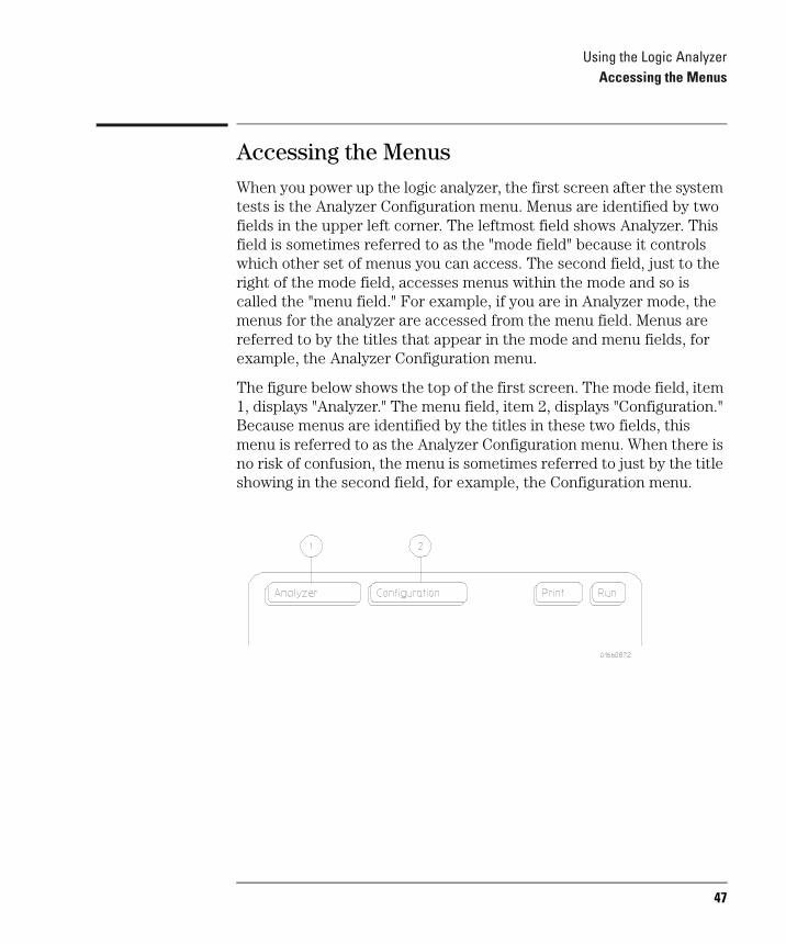
Accessing the MenusWhen you power up the logic analyzer, the first screen after the system tests is the Analyzer Configuration menu. Menus are identified by two fields in the upper left corner. The leftmost field shows Analyzer. This field is sometimes referred to as the "mode field" because it controls which other set of menus you can access. The second field, just to the right of the mode field, accesses menus within the mode and so is called the "menu field." For example, if you are in Analyzer mode, the menus for the analyzer are accessed from the menu field. Menus are referred to by the titles that appear in the mode and menu fields, for example, the Analyzer Configuration menu.
The figure below shows the top of the first screen. The mode field, item 1, displays "Analyzer." The menu field, item 2, displays "Configuration." Because menus are identified by the titles in these two fields, this menu is referred to as the Analyzer Configuration menu. When there is no risk of confusion, the menu is sometimes referred to just by the title showing in the second field, for example, the Configuration menu.
47
Using the Logic AnalyzerAccessing the Menus
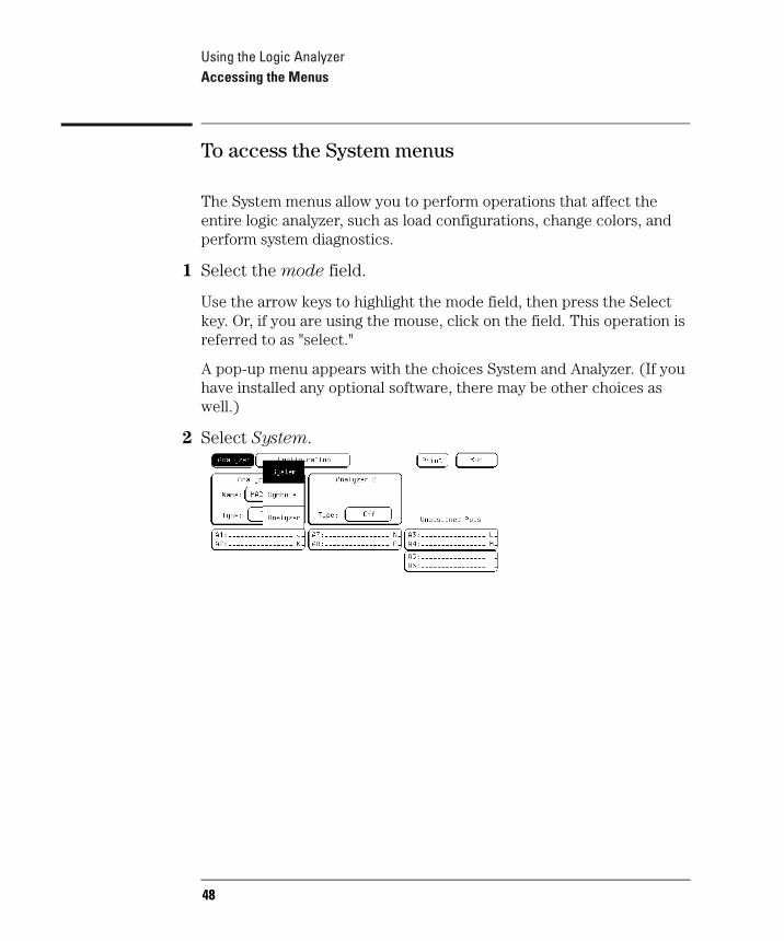
To access the System menus
The System menus allow you to perform operations that affect the entire logic analyzer, such as load configurations, change colors, and perform system diagnostics.
1 Select the mode field.
Use the arrow keys to highlight the mode field, then press the Select key. Or, if you are using the mouse, click on the field. This operation is referred to as "select."
A pop-up menu appears with the choices System and Analyzer. (If you have installed any optional software, there may be other choices as well.)
2 Select System.
48

Using the Logic AnalyzerAccessing the Menus
3 Select the menu field.
The pop-up lists five menus: Hard Disk, Flexible Disk, External I/O, Utilities, and Test.
• Hard Disk allows you to perform file operations on the hard disk.
• Flexible Disk allows you to perform file operations on the flexible disk.
• External I/O allows you to configure your GPIB, RS-232-C, and LAN interfaces, connect to a printer and controller, and to reset the 1670G-series logic analyzer.
• Utilities allows you to set the clock, update the operating system software, and adjust the display.
• Test displays the installed software version number and loads the self tests.
See Also For information on "File Management" see page 134, and for information on "Disk Drive Operations" see page 275.
For information on the External I/O menu, "Connecting Peripherals", see page 35, and "The RS-232-C, GPIB, and Centronics Interfaces" see page 282.
49
Using the Logic AnalyzerAccessing the Menus
To access the Analyzer menus
The Analyzer menus allow you to control the analyzer to make your measurement, perform operations on the data, and view the results on the display.
1 Select the mode field.
A pop-up menu appears with the choices System, Analyzer, and Patt Gen or Scope (if you have one of these options). If you have installed any optional software, there may be other choices as well.
2 Select Analyzer.
3 Select the menu field.
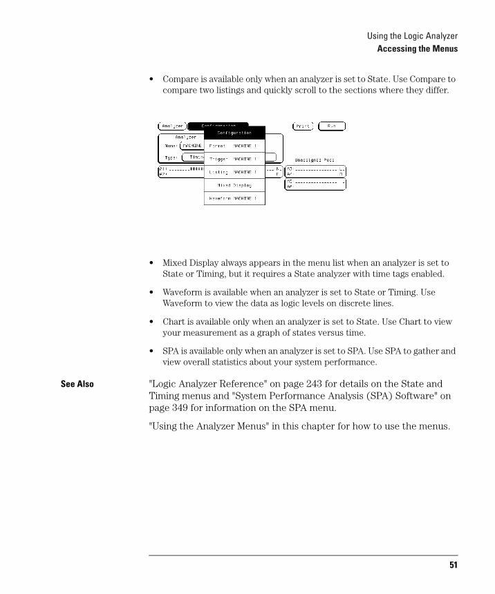
The figure on the next page does not show all of the possible menus because certain menus are only accessible with the analyzer configured in a particular mode. For instance, the Compare menu is only available when you set an analyzer to state mode, and the SPA menu requires an analyzer set to SPA.
• Configuration is always available in Analyzer mode. Use Configuration to assign pods and set the analyzer type.
• Format is available whenever an analyzer is set to a type other than "Off." Use Format to create data labels and symbols, adjust the pod threshold level, and set modes and clocks.
• Trigger is available when an analyzer is set to State or Timing. Use Trigger to specify a trigger sequence which will filter the raw information into the measurement you want to see.
• Listing is available when an analyzer is set to State or Timing. Use Listing to view your measurement as a list of states. Using an inverse assembler, a state analyzer can display the measurement as though it were assembly code.
50
Using the Logic AnalyzerAccessing the Menus
• Compare is available only when an analyzer is set to State. Use Compare to compare two listings and quickly scroll to the sections where they differ.
• Mixed Display always appears in the menu list when an analyzer is set to State or Timing, but it requires a State analyzer with time tags enabled.
• Waveform is available when an analyzer is set to State or Timing. Use Waveform to view the data as logic levels on discrete lines.
• Chart is available only when an analyzer is set to State. Use Chart to view your measurement as a graph of states versus time.
• SPA is available only when an analyzer is set to SPA. Use SPA to gather and view overall statistics about your system performance.
See Also "Logic Analyzer Reference" on page 243 for details on the State and Timing menus and "System Performance Analysis (SPA) Software" on page 349 for information on the SPA menu.
"Using the Analyzer Menus" in this chapter for how to use the menus.
51
Using the Logic AnalyzerUsing the Analyzer Menus
Using the Analyzer MenusThe following examples show how to use some of the Analyzer menus to configure the logic analyzer for measurements. These examples assume that you have already determined which signals are of interest, and have connected the logic analyzer to the target system. Some of the examples use data from a Motorola 68360 target system, acquired with an Agilent Technologies E2456A Analysis Probe.
To label channel groups
Agilent Technologies logic analyzers give you the ability to separate or group data channels and label the groups with a name that is meaningful to your measurement. Labels also assist you in triggering only on states of interest.
Labels can only be assigned in the Analyzer Format menu. Once assigned, the labels are available in all display menus, where they can be added to or deleted from the display. Use labels when you want to group data channels by function with a name that has meaning to that function.
The default label names are Bus1 through Bus126. However, you can modify a name to any six-character string. If you are using an Agilent Technologies analysis probe, the configuration file has predefined labels for your specific processor.
52
Using the Logic AnalyzerUsing the Analyzer Menus
To create or modify a label and assign channel groups, use the following procedure.
1 Press the Format key to go to the Format menu.
2 Select a label under the Labels heading. In the pop-up menu, select Modify Label.
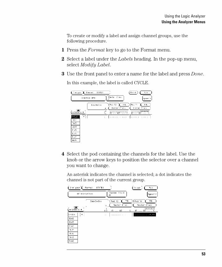
3 Use the front panel to enter a name for the label and press Done.
In this example, the label is called CYCLE.
4 Select the pod containing the channels for the label. Use the knob or the arrow keys to position the selector over a channel you want to change.
An asterisk indicates the channel is selected; a dot indicates the channel is not part of the current group.
53
Using the Logic AnalyzerUsing the Analyzer Menus
5 Toggle the channel's group status by pressing Select.
The indicator changes and the selector moves to the next channel.
6 Press the Done key to complete selection.
54
Using the Logic AnalyzerUsing the Analyzer Menus
To create a symbol
Symbols are alphanumeric mnemonics that represent specific data patterns or ranges. When you define a symbol and set the base type to Symbol in the Listing menu, the symbol is displayed in the data listing where the bit pattern would normally be displayed. The symbols also appear in the Waveform menu when you view a label in bus form. Symbols allow you to quickly identify data of interest.
To create a symbol, use the following procedure.
1 In the Analyzer Format menu, select Symbols.
The symbol table menu appears. The symbol table is where all user symbols are created and maintained. If you get a message, "No labels specified," check that you have at least one label turned on with channels assigned to it.
2 In the Symbol menu, select the Label field. In the pop-up menu, select the label that contains the channel groups you want.
When you open the symbol table menu, the Label field displays the name of the first active label.
If the label you want does not appear in the pop-up menu, the label is probably off. Return to the Format menu, select the label you want, and select Turn Label On. Another possibility is that the label is on the other analyzer. The two analyzers manage resources separately.
3 Select the Base field. In the pop-up menu, select the base for the pattern.
In this example, binary is used because CYCLE only contains three channels.
4 Select the field below Symbol. Select Add a Symbol, type in the symbol name, then press Done.
55
Using the Logic AnalyzerUsing the Analyzer Menus
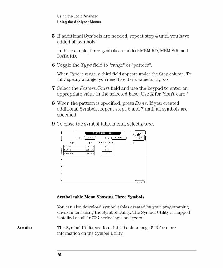
5 If additional Symbols are needed, repeat step 4 until you have added all symbols.
In this example, three symbols are added: MEM RD, MEM WR, and DATA RD.
6 Toggle the Type field to "range" or "pattern".
When Type is range, a third field appears under the Stop column. To fully specify a range, you need to enter a value for it, too.
7 Select the Pattern/Start field and use the keypad to enter an appropriate value in the selected base. Use X for "don't care."
8 When the pattern is specified, press Done. If you created additional Symbols, repeat steps 6 and 7 until all symbols are specified.
9 To close the symbol table menu, select Done.
Symbol table Menu Showing Three Symbols
You can also download symbol tables created by your programming environment using the Symbol Utility. The Symbol Utility is shipped installed on all 1670G-series logic analyzers.
See Also The Symbol Utility section of this book on page 563 for more information on the Symbol Utility.
56
Using the Logic AnalyzerUsing the Analyzer Menus
To examine an analyzer waveform
The Analyzer Waveform menu lets you view state or timing data in a format similar to an oscilloscope display. The horizontal axis represents states (in state mode) or time (in timing mode) and the vertical axis represents logic highs and lows.
1 In Analyzer mode, press the Run key to acquire data.
In any mode other than Analyzer, Scope, or Patt Gen, pressing the Run key has no effect. The menus which ignore Run, lack the Run field onscreen. In Analyzer mode with Run available, the menu changes to a display menu.
2 Go to the Analyzer Waveform menu.
3 To adjust the horizontal axis (sec/Div or states/Div), use the knob.
If nothing happens when you turn the knob, make sure the Div field has a roll indicator above it, as in the figures on the next page. When you first enter the Waveform menu, the knob adjusts the horizontal axis but if you select another rollable field, the knob will control that field instead.
4 To adjust the display relative to the trigger, select the Delay field and enter a value or use the knob.
The portion of memory being displayed is indicated by a white bar along the bottom of the display area. The position of the trigger in memory is indicated by a red dot on the same line. When the bar includes the dot, then the trigger is visible on the display as indicated by a vertical line with a "t" underneath.
57
Using the Logic AnalyzerUsing the Analyzer Menus
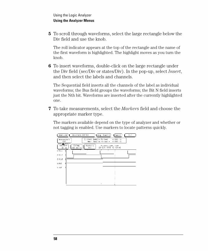
5 To scroll through waveforms, select the large rectangle below the Div field and use the knob.
The roll indicator appears at the top of the rectangle and the name of the first waveform is highlighted. The highlight moves as you turn the knob.
6 To insert waveforms, double-click on the large rectangle under the Div field (sec/Div or states/Div). In the pop-up, select Insert, and then select the labels and channels.
The Sequential field inserts all the channels of the label as individual waveforms; the Bus field groups the waveforms; the Bit N field inserts just the Nth bit. Waveforms are inserted after the currently highlighted one.
7 To take measurements, select the Markers field and choose the appropriate marker type.
The markers available depend on the type of analyzer and whether or not tagging is enabled. Use markers to locate patterns quickly.
58
Using the Logic AnalyzerUsing the Analyzer Menus
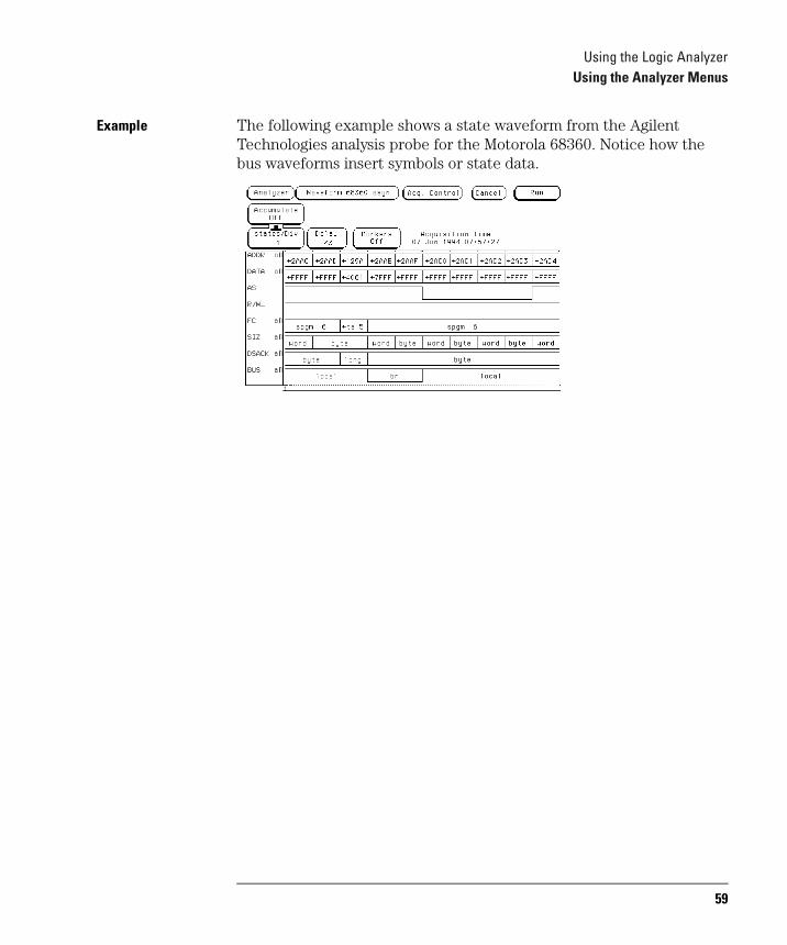
Example The following example shows a state waveform from the Agilent Technologies analysis probe for the Motorola 68360. Notice how the bus waveforms insert symbols or state data.
59
Using the Logic AnalyzerUsing the Analyzer Menus
To examine an analyzer listing
The Analyzer Listing menu displays state or timing data as patterns (states). The Listing menu uses any of several formats to display the data such as binary, ASCII, or symbols. If you are using an inverse assembler and select Invasm, the data is displayed in mnemonics that closely resemble the microprocessor source code.
See Also "The Inverse Assembler" at the end of this chapter for additional information on using an inverse assembler.
1 In Analyzer mode, press the Run key to acquire data.
In any mode other than Analyzer, Scope, or Patt Gen, pressing the Run key has no effect. The menus which ignore Run lack the Run field onscreen. In Analyzer mode with Run available, the menu changes to a display menu.
2 Go to the Analyzer Listing menu.
All labels defined in the Analyzer Format menu appear in the listing. If there are more labels than will fit on the screen, the Label/Base field is shaded like a normal field.
3 To scroll the labels, select the Label/Base field and use the knob or press the blue shift key and a page key.
If the Label/Base field is selectable, the roll indicator appears over the field as in the example. To move the labels one full screen at a time, press Shift and a Page key.
60
Using the Logic AnalyzerUsing the Analyzer Menus
4 To scroll the data, use the Page keys or select the data roll field and use the knob.
If you select the data roll field, the roll indicator moves to it. No matter which field is currently controlled by the knob, however, the Page keys page the data up or down.
The numbers in the data roll column indicate how many samples the data is from the trigger. Negative numbers occurred before the trigger and positive numbers occurred after.
5 If the labels have symbols associated with them, set the base to Symbol.
The symbols you defined appear in the listing.
6 To insert a label, select one of the label fields, then select Insert from the pop-up and the label you want to insert.
The last label cannot be deleted, so there is always at least one label. You can insert the same label multiple times and display it in different bases.
7 To take measurements, select the Markers field and choose the appropriate marker type.
The markers available depend on the type of analyzer and whether or not tagging is enabled. Use markers to locate states quickly.
61

Using the Logic AnalyzerUsing the Analyzer Menus
Example The following illustration shows a listing from the Agilent Technologies analysis probe for the Motorola 68360. The ADDR label has the base set to Hex to conserve space on the display. The DATA label has the base set to Invasm for inverse assembly. The FC label has the base set to Symbol. Additional labels are located to the right of FC, and can be viewed by highlighting and selecting Label, then using the knob to scroll the display horizontally.
62

Using the Logic AnalyzerUsing the Analyzer Menus
To compare two listings
The Compare menu allows you to take two state analyzer acquisitions and compare them to find the differences. You can use this function to quickly find all the effects after changing the target system or to quickly compare the results of quality tests with results from a working system.
1 In Analyzer mode, press the Run key to acquire data.
In any mode other than Analyzer, Scope, or Patt Gen, pressing the Run key has no effect. The menus which ignore Run lack the Run field onscreen. In Analyzer mode with Run available, the menu changes to a display menu.
2 Go to the Analyzer Compare menu, select Copy Listing to
Reference, and then select Execute.
The Compare menu initially is empty, but when you select Execute the data appears.
3 Set up the other test that you want to compare to the first.
This can be a change to the hardware, or a different system. Do not change the trigger, however, or all the states will be different.
4 Run the test again, then select the Reference listing field to toggle to Difference listing.
The Difference listing is displayed on the next page.
63
Using the Logic AnalyzerUsing the Analyzer Menus
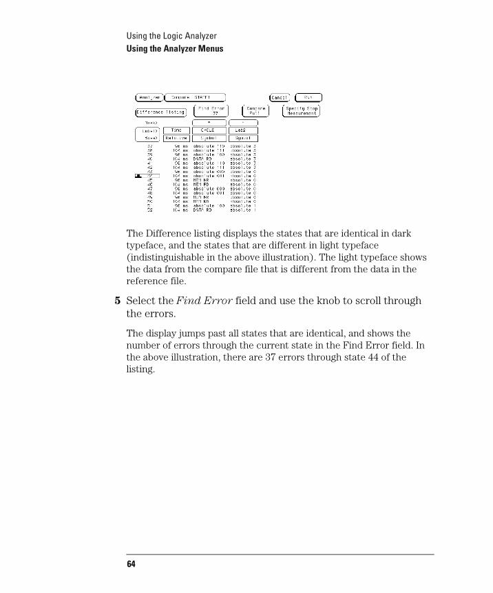
The Difference listing displays the states that are identical in dark typeface, and the states that are different in light typeface (indistinguishable in the above illustration). The light typeface shows the data from the compare file that is different from the data in the reference file.
5 Select the Find Error field and use the knob to scroll through the errors.
The display jumps past all states that are identical, and shows the number of errors through the current state in the Find Error field. In the above illustration, there are 37 errors through state 44 of the listing.
64
Using the Logic AnalyzerThe Inverse Assembler
The Inverse AssemblerWhen the analyzer captures a trace, it captures binary information. The analyzer can then present this information in symbol, binary, octal, decimal, hexadecimal, or ASCII. Or, if given information about the meaning of the data captured, the analyzer can inverse assemble the trace. The inverse assembler makes the trace list more readable by presenting the trace results in terms of processor opcodes and data transactions.
To use an inverse assembler
Most analysis probes include an inverse assembler in their software. Loading the configuration file for the analysis probe sets up the logic analyzer to provide certain types of information for the inverse assembler. This section is provided in case you ever have to set up an analyzer for inverse assembly yourself.
The inverse assembly software needs at least these five pieces of information:
• Address bus. The inverse assembler expects to see the label ADDR, with bits ordered in a particular sequence.
• Data bus. The inverse assembler expects to see the label DATA, with bits ordered in a particular sequence.
• Status. The inverse assembler expects to see the label STAT, with bits ordered in a particular sequence.
• Start state for disassembly. This is the first displayed state in the trace list, not the cursor position. See the figure on the next page.
• Tables indicating the meaning of particular status and data combinations.
65
Using the Logic AnalyzerThe Inverse Assembler
The particular sequences that each label requires depends on the type of chip the inverse assembler was designed for. Because of this, inverse assemblers cannot generally be transferred between platforms.
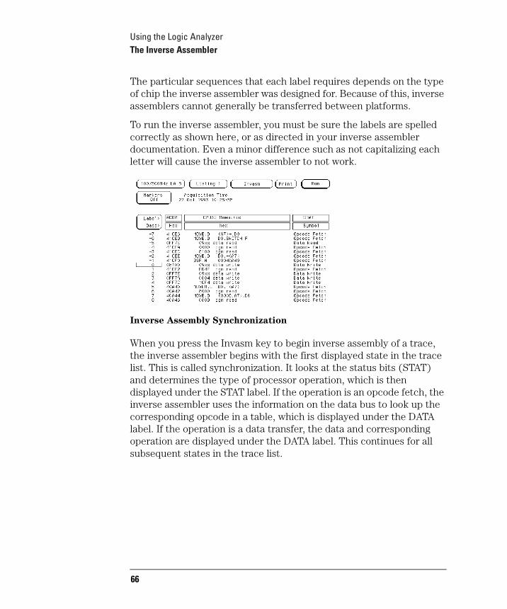
To run the inverse assembler, you must be sure the labels are spelled correctly as shown here, or as directed in your inverse assembler documentation. Even a minor difference such as not capitalizing each letter will cause the inverse assembler to not work.
Inverse Assembly Synchronization
When you press the Invasm key to begin inverse assembly of a trace, the inverse assembler begins with the first displayed state in the trace list. This is called synchronization. It looks at the status bits (STAT) and determines the type of processor operation, which is then displayed under the STAT label. If the operation is an opcode fetch, the inverse assembler uses the information on the data bus to look up the corresponding opcode in a table, which is displayed under the DATA label. If the operation is a data transfer, the data and corresponding operation are displayed under the DATA label. This continues for all subsequent states in the trace list.
66
Using the Logic AnalyzerThe Inverse Assembler
If you roll the trace list to a new position and press Invasm again, the inverse assembler repeats the above process. However, it does not work backward in the trace list from the starting position. This may cause differences in the trace list above and below the point where you synchronized inverse assembly. The best way to ensure correct inverse assembly is to synchronize using the first state you know to be the first byte of an opcode fetch.
See Also The Analysis Probe User's Guide for more information on controlling inverse assembly. If you have problems using the inverse assembler, see "Troubleshooting the Logic Analyzer" on page 421.
67

Using the Logic AnalyzerThe Inverse Assembler
68
4
Using the Trigger Menu
69

Using the Trigger MenuUsing the Trigger Menu
Using the Trigger MenuTo use the logic analyzer efficiently, you need to be able to set up your own triggers. This chapter provides examples of triggering. Those examples assume you already know where to find fields in the trigger menu.
This chapter shows you how to:
• Specify a basic trigger
• Change a trigger sequence
• Set up time correlation between analyzers
• Arm from another instrument, or arm another instrument
• Manage memory
70
Using the Trigger MenuSpecifying a Basic Trigger
Specifying a Basic TriggerThe default analyzer triggers are
While storing "anystate" TRIGGER on "a" occuring 1 timeStore "anystate"
for state analyzers and
TRIGGER on "a" > 8 ns
for timing analyzers. If you want to simply record data, these will get you started. They can quickly be tailored by specifying a particular pattern to look for instead of the general case.
Customizing a trigger generally requires these steps:
• Assign terms.
• Define the terms.
• Change the trigger to use the new terms.
71
Using the Trigger MenuSpecifying a Basic Trigger
To assign terms to an analyzer
When you turn the logic analyzer on, Analyzer 1 is named Machine 1 and Analyzer 2 is off. Because trigger terms can only be used by one analyzer at a time, all the terms are assigned to Analyzer 1. If you plan to use both analyzers in your measurement, you need to assign some of the terms to Analyzer 2.
1 Go to the Trigger Machine 1 menu.
If you have renamed Machine 1 in the Analyzer Configuration menu, the name you changed it to will appear in the menu instead of Machine 1.
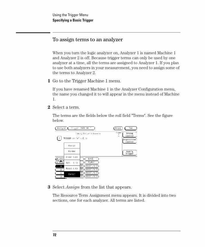
2 Select a term.
The terms are the fields below the roll field "Terms". See the figure below.
3 Select Assign from the list that appears.
The Resource Term Assignment menu appears. It is divided into two sections, one for each analyzer. All terms are listed.
72

Using the Trigger MenuSpecifying a Basic Trigger
4 To change a term assignment, select the term field.
The term fields toggle from one section to the other. You can get all your terms assigned at once, or just change a few to meet immediate needs.
5 To exit the term assignment menu, select Done.
73
Using the Trigger MenuSpecifying a Basic Trigger
To define a term
Both default triggers trigger on term "a". If you only need to look for the occurrence of a certain state, such as a write to protected memory, then you only need to define term "a" to make the measurement you want.
1 In the Trigger menu, select the field at the intersection of the term and the label whose value you want to trigger on.
You set labels in the Analyzer Format menu. If the channels you want to monitor are not attached to a label, they will not appear in the trigger menu.
2 Enter the value or pattern you want to trigger on.
If the label's base is Symbol, a pop-up menu appears offering a choice of symbols. For other bases, use the keypad. An "X" stands for "don't care".
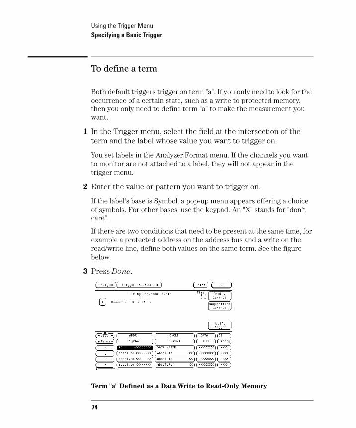
If there are two conditions that need to be present at the same time, for example a protected address on the address bus and a write on the read/write line, define both values on the same term. See the figure below.
3 Press Done.
Term "a" Defined as a Data Write to Read-Only Memory
74
Using the Trigger MenuSpecifying a Basic Trigger
To change the trigger specification
Most triggers use terms other than "a." Even a simple trigger might use additional terms to set conditions on the actual trigger. To use these terms, you must include them in the trigger sequence specification.
1 In the Trigger menu, select the number beside the specific level you want to modify.
A Sequence Level menu pops up. It shows the current specification for that trigger level.
2 Select the field you want to change.
In the top row of the pop-up are three action fields: Insert Level, Select New Function, and Delete Level. The next section goes into detail on them. The fields after "While storing", "TRIGGER on", and "Else on" are completed with trigger terms. Selecting these fields pops up a menu of terms.
3 Select the term you want to use from the pop-up, or enter a new value, as appropriate to the field.
If you have renamed a term, that name is automatically used everywhere the term would appear.
75
Using the Trigger MenuSpecifying a Basic Trigger
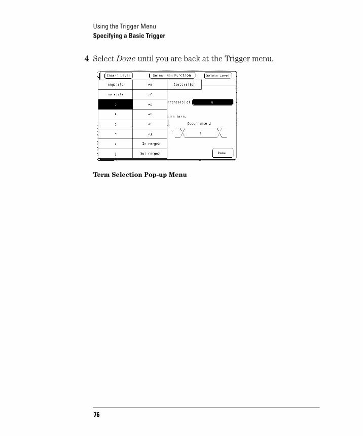
4 Select Done until you are back at the Trigger menu.
Term Selection Pop-up Menu
76
Using the Trigger MenuChanging the Trigger Sequence
Changing the Trigger SequenceMost measurements require more complicated triggers to better filter information. From the basic trigger, you can:
• Add sequence levels
• Change trigger functions
Your logic analyzer provides a trigger function library to make setting up the trigger easier. There are 12 state functions and 13 timing functions. Most trigger functions take more than one level internally to implement, and can be broken down into their separate levels. Once broken down, the levels can be used to design your own trigger sequences.
77
Using the Trigger MenuChanging the Trigger Sequence
To add sequence levels
You can add sequence levels anywhere except after the final one.
1 In the Trigger menu, select the number beside the sequence level just after where you want to insert.
For example, if you want to insert a sequence level between levels 1 and 2, you would select level 2. To insert levels at the beginning, select level 1.
A Sequence Level pop-up appears. Its exact contents depend on the analyzer configuration and the level specification. However, all Sequence Level pop-ups have an Insert Level field in the upper left corner.
2 Select Insert Level.
Another pop-up offers the choices of Cancel, Before, or After. If the level you started from was the last level, After will not appear.
3 Select Before.
The Trigger Function pop-up replaces the Sequence Level pop-up. The functions available depend on whether the analyzer is configured as state or timing.
4 Use the knob to highlight a trigger function, and select Done.
A new Sequence level pop-up appears. Its contents reflect the trigger function you just selected. The figure below shows a user trigger function for a state analyzer.
78

Using the Trigger MenuChanging the Trigger Sequence
5 Fill in the fields and select Done.
Sequence Level Pop-up Menu
79
Using the Trigger MenuChanging the Trigger Sequence
To change trigger functions
You do not need to add and delete levels just to change a level's trigger function. This can be done from within the Sequence Level pop-up.
1 From the Trigger menu, select the sequence level number of the sequence level you want to modify.
A Sequence Level pop-up appears. Its contents reflect the current trigger function.
2 Select Select New Function.
The Trigger Function pop-up replaces the Sequence Level pop-up. The functions available depend on whether the analyzer is configured as state or timing.
3 Use the knob to highlight the function you want, and select Done.
A new Sequence Level pop-up appears. Its contents reflect the function you just selected. The wording of this screen is very similar to the function description, and the line drawing demonstrates what the function is measuring.
4 Select the appropriate assignment fields and insert the desired pre-defined terms, numeric values, and other parameter fields required by the function. Select Done.
For state analyzers, a final "go to trigger" level is automatically placed at the end of the trigger specification for you. This level must always be a user level. Although you can change its fields, you cannot change the function. Timing analyzers do not have this restriction.
See Also "Timing Trigger Function Library" and "State Trigger Function Library" in The Analyzer Trigger Menu on page 312 for a complete listing of functions.
80
Using the Trigger MenuSetting Up Time Correlation between Analyzers
Setting Up Time Correlation between AnalyzersThere are two possible combinations of analyzers: state and state, and state and timing. Timing and timing is not possible because the Analyzer Configuration menu only permits one analyzer at a time to be configured as a timing analyzer. For either combination, time correlation is necessary for interleaving and mixed display.
Time correlation is useful when you want to store different sorts of data for each trace, but see how they are related. For instance, you could set up a timing and a correlated state analyzer and see if setup and hold times are being met. Or, you could set up two state analyzers and have one watch normal program execution and the other watch the control and status lines.
Time correlation requires that state analyzers store time tags. You set the state analyzer to store time tags by turning on Count Time in the Analyzer Trigger menu. The timing analyzer already stores time tags when it samples data.
See Also "Special displays" on page 128 for more information on interleaving and mixed display.
81
Using the Trigger MenuSetting Up Time Correlation between Analyzers
To set up time correlation between two state analyzers
To correlate the data between two state analyzers, both must have Count Time turned on in their Trigger menus. Although both have Count State available, it is not possible to correlate data based on states even when they are identically defined.
1 In the Analyzer Trigger menu, select Count.
Count may be Count Off, Count Time, or Count States. Selecting the field causes a pop-up to appear.
2 Select the field after Count: and select Time.
A warning may appear about reduced memory. It will not prevent you from changing Count to Count Time.
3 Select Done.
4 Repeat steps 1 through 3 for the other state analyzer.
Now when you acquire data you will be able to interleave the listings.
82
Using the Trigger MenuSetting Up Time Correlation between Analyzers
To set up time correlation between a timing and a state analyzer
To set up time correlation between a timing and a state analyzer, only the state analyzer needs to have Count Time turned on. The timing analyzer automatically keeps track of time.
1 In the state Analyzer Trigger menu, select Count.
Count may be Count Off, Count Time, or Count States. Selecting the field causes a pop-up to appear.
2 Select the field after Count: and select Time.
A warning may appear about reduced memory. It will not prevent you from changing Count to Count Time.
3 Select Done.
Now when you acquire data you will be able to set up a mixed display.
83
Using the Trigger MenuArming and Additional Instruments
Arming and Additional InstrumentsOccasionally you may need to start the analyzer acquiring data when another instrument detects a problem. Or, you may want to have the analyzer itself arm another measuring tool. This is accomplished from the Arming Control field of the Analyzer Trigger menu.
To arm another instrument
1 Attach a BNC cable from the External Trigger Output port on the back of the logic analyzer to the instrument you want to trigger.
The External Trigger Output port is also referred to as "Port Out." It uses standard TTL logic signal levels, and will generate a rising edge when trigger conditions are met.
2 In the Analyzer Trigger menu, select Arming Control.
Arming Control is below the Run button.
3 Select the field near Arm Out, and choose PORT OUT.
4 If you are using both analyzers, set the Arm Out Sent From field in the upper right corner.
This field does not appear if only one analyzer is configured.
The selected analyzer will send the arm signal when it finds its trigger.
5 Select Done.
When you make a measurement, the analyzer will send an arm signal through the External Trigger Output when the analyzer finds its trigger.
84
Using the Trigger MenuArming and Additional Instruments
To arm the oscilloscope with the analyzer (1670G-series logic analyzers with the oscilloscope option)
If both analyzer and the oscilloscope are turned on, you can configure one analyzer to arm the other analyzer and the oscilloscope. An example of this is when a state analyzer triggers on a bit pattern, then arms a timing analyzer and the oscilloscope which capture and display the waveform after they trigger.
1 In the Analyzer Trigger menu, select Arming Control.
2 Select the Analyzer Arm Out Sent From field, and choose from the list the Analyzer that will generate the arm.
3 Select the Analyzer Arm In field, and choose Group Run.
This allows you to time-correlate the data from the analyzers and the scope. The Scope Trigger Mode must be Immediate for correlation.
4 Select the field of the instrument which will arm the others, and in the pop-up set it to run from Group Run.
The Scope field is not selectable. To set how the scope is run, select the field under Scope Arm In.
5 Select the other instrument fields and choose the mechanism which will arm them.
The Analyzer Arm Out field determines which analyzer sends the arming signal to Port Out and to the oscilloscope if the oscilloscope is being armed by an analyzer.
As you set each machine, the arrows connecting the fields in the Arming Control menu change. The arrows show the order in which the instruments are armed.
See the example on the next page.
6 Select Done until you are back at the Trigger menu.
85
Using the Trigger MenuArming and Additional Instruments
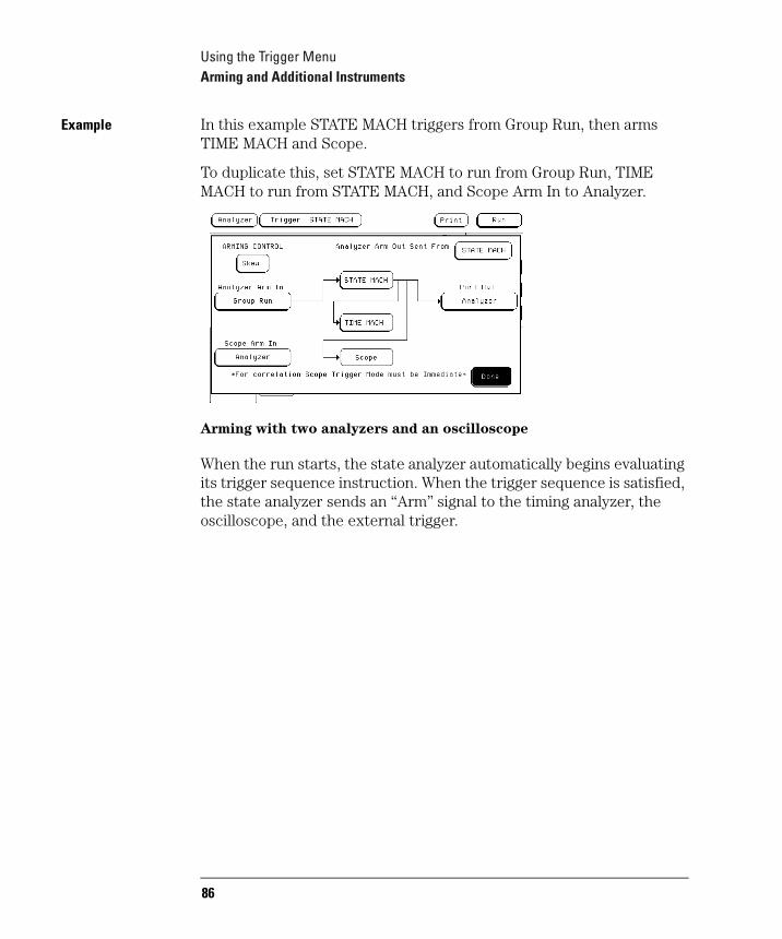
Example In this example STATE MACH triggers from Group Run, then arms TIME MACH and Scope.
To duplicate this, set STATE MACH to run from Group Run, TIME MACH to run from STATE MACH, and Scope Arm In to Analyzer.
Arming with two analyzers and an oscilloscope
When the run starts, the state analyzer automatically begins evaluating its trigger sequence instruction. When the trigger sequence is satisfied, the state analyzer sends an “Arm” signal to the timing analyzer, the oscilloscope, and the external trigger.
86
Using the Trigger MenuArming and Additional Instruments
To receive an arm signal from another instrument
When you set the analyzer to wait for an arm signal, it does not react to data that would normally trigger it until after it has received the arm signal. The arm signal can be sent to any of the Trigger Sequence levels, but will go to level 1 unless you change it. Setting up the analyzer to receive an arm signal is more efficient when the sequence levels are already in place.
1 Connect a BNC cable from the instrument which will be sending the signal to the External Trigger Input port on the back of the logic analyzer.
CAUTION: Do not exceed 5.5 volts on the External Trigger Input.
The External Trigger Input port is also referred to as "Port In." It uses standard TTL logic signal levels, and expects a rising edge as input.
2 In the Analyzer Trigger menu, select Arming Control.
Arming Control is below the Run button.
3 Select the leftmost field, and choose PORT IN.
The field is unlabeled and shows either Run or PORT IN. It has arrows going from it to the analyzer(s).
!
87
Using the Trigger MenuArming and Additional Instruments
4 To change the default settings, select the analyzer field.
A small pop-up menu appears. To change which device the analyzer is receiving its arm signal from, select the Run from field. To change which sequence level is waiting for the arm signal, select the Arm sequence level field.
5 Select Done until you are back at the Trigger menu.
88
Using the Trigger MenuManaging Memory
Managing MemorySometimes you will need every last bit of memory you can get on the logic analyzer. There are three simple ways to maximize memory when specifying your trigger:
• Selectively store branch conditions (state only)
• To set the memory length
• Place the trigger relative to memory
• Set the sampling rates (timing only)
89
Using the Trigger MenuManaging Memory
To selectively store branch conditions (state only)
Besides setting up your trigger levels to store anystate, no state, or some subset of states, you can also choose whether or not to store branch conditions. Branch conditions are always stored by default, and can make tracing the analyzer's path through a complicated trigger easier. If you really need the extra memory, however, it is possible to not store the branch conditions.
You cannot set the analyzer to store only some branches in a trigger sequence specification.
1 In the Analyzer Trigger menu, select Acquisition Control.
The Acquisition Control menu pops up. If the acquisition mode is set to Automatic, the menu contains a single field and an explanation. If Acquisition has been customized, it has 3 fields and a picture showing where the trigger is currently placed in memory.
2 If the mode is Automatic, select the field and toggle it to Manual.
The menu now shows three fields and a picture.
3 Select the Branches Taken Stored field.
It toggles to Branches Taken Not Stored.
4 Select Done.
90
Using the Trigger MenuManaging Memory
To set the memory length
The 1670G-series logic analyzer’s memory length can be adjusted. The table on the following page shows the amount of memory available for different modes of operation.
Typically you will want to use small amounts of memory at the beginning of troubleshooting, when you are first looking for a problem, and use deep memory when you are searching for the root cause. Shallower memory provides faster acquisitions, but might not have sufficient context. Deep memory provides more context, but takes longer to fill, more time to display, and more time for you to analyze. The Memory Length field allows you to configure the acquisition memory to suit your needs.
1 In the Analyzer Trigger menu, select Acquisition Control.
The Acquisition Control menu pops up. If the acquisition mode is set to Automatic, the menu contains two fields and an explanation. If Acquisition has been customized, it has four or five fields and a picture showing the amount of memory and where the trigger is currently placed in memory.
2 Select the Memory Length field.
Use the knob to select the memory length. Memory size can be set in powers of 2 from 4096 to the maximum. The table below shows the maximum memory for various modes of operation.
91
Using the Trigger MenuManaging Memory
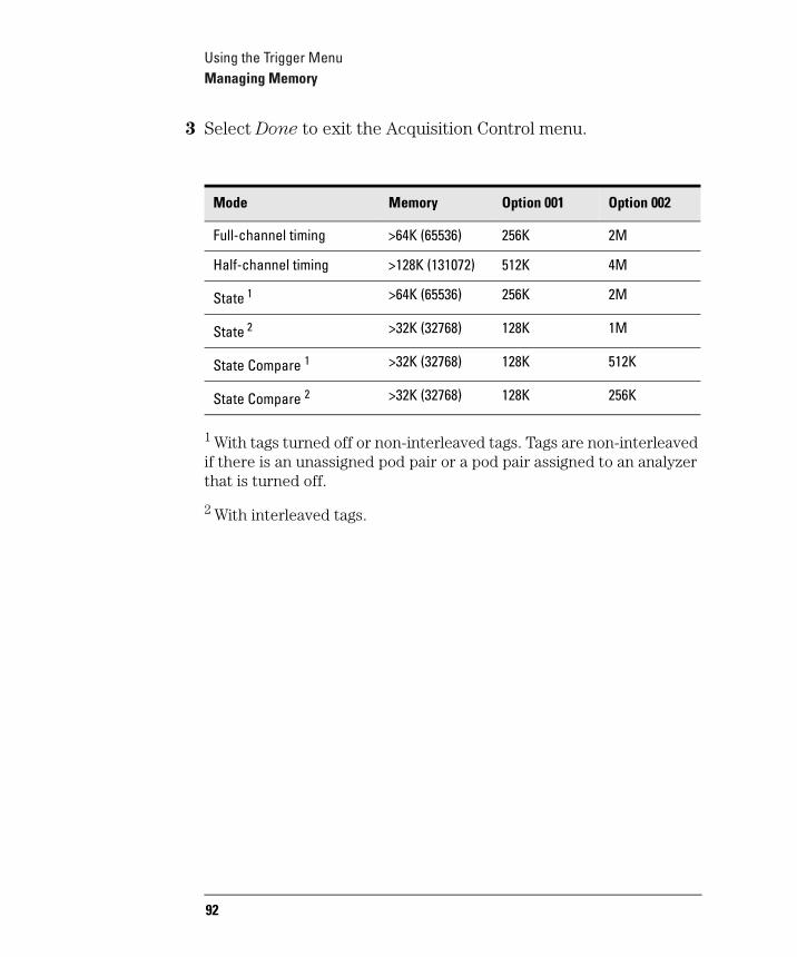
3 Select Done to exit the Acquisition Control menu.
1 With tags turned off or non-interleaved tags. Tags are non-interleaved if there is an unassigned pod pair or a pod pair assigned to an analyzer that is turned off.
2 With interleaved tags.
Mode Memory Option 001 Option 002
Full-channel timing >64K (65536) 256K 2M
Half-channel timing >128K (131072) 512K 4M
State 1 >64K (65536) 256K 2M
State 2 >32K (32768) 128K 1M
State Compare 1 >32K (32768) 128K 512K
State Compare 2 >32K (32768) 128K 256K
92
Using the Trigger MenuManaging Memory
To place the trigger in memory
In Automatic Acquisition Mode, the exact location of the trigger depends on the trigger specification but usually falls around the center. You can manually place it at the beginning, end, or anywhere else.
1 In the Analyzer Trigger menu, select Acquisition Control.
The Acquisition Control menu pops up. If the acquisition mode is set to Automatic, the menu contains a single field and an explanation. If Acquisition has been customized, it has 3 or 4 fields and a picture showing where the trigger is currently placed in memory.
2 If the mode is Automatic, select the field to toggle it to Manual.
The menu now shows three fields and a picture.
3 Select the Trigger Position field.
4 Select the appropriate entry for your needs.
Start, Center, and End place the trigger respectively at the beginning, middle, and end of the memory. Delay, available in timing analyzers only, causes the analyzer to not save any data before the time delay has elapsed. User Defined calls up a fourth field where you specify exactly where you want the trigger.
5 Select Done.
93
Using the Trigger MenuManaging Memory
To set the sampling rates (Timing only)
A timing analyzer samples the data based on its own internal clock. A short sample period provides more detail about the device under test; a long sample period allows more time before memory is full. However, if the sample period is too large, some information may be missed.
1 In the Analyzer Trigger menu, select Acquisition Control.
The Acquisition Control menu pops up. If the acquisition mode is set to Automatic, the menu contains a single field and an explanation. If Acquisition has been customized, it has 3 or 4 fields and a picture showing where the trigger is currently placed in memory.
2 If the mode is Automatic, select the field and toggle it to Manual.
The menu now shows three fields and a picture.
3 Set the Sample Period field using the knob, or select it to use the keypad to enter the period.
4 Select Done.
Next time you take a measurement, the analyzer will sample at the rate you entered.
94
5
Triggering Examples
95
Triggering ExamplesTriggering Examples
Triggering ExamplesAs you begin to understand a problem in your system, you may realize that certain conditions must occur before the problem occurs. You can use sequential triggering to ensure that those conditions have occurred before the analyzer recognizes its trigger and captures information.
If you are not familiar with the trigger menus, read through Chapter 4, "Using the Trigger Menu," and try working through the examples in the Logic Analyzer Training Kit manual.
96
Triggering ExamplesSingle-Machine Trigger Examples
Single-Machine Trigger ExamplesThe following examples require only a single analyzer to make measurements. Sequence specifications are given in the form you see within the sequence levels, but the illustrations show the complete, multi-level sequence specification.
Although all the examples are case-specific, terms are named in a way that highlights their role in solving the trigger problem. You can easily apply the examples to your specific instance by changing the specific values assigned to the trigger terms.
97
Triggering ExamplesSingle-Machine Trigger Examples
To store and time the execution of a subroutine
Most system software of any kind is composed of a hierarchy of functions and procedures. During integration, testing, and performance evaluation, you want to look at specific procedures to verify that they are executing correctly and that the implementation is efficient. The analyzer lets you do this by triggering on entry to the address range of the subroutine and counting the elapsed time since the trigger state.
1 Go to the state analyzer's Trigger menu.
2 Set Count to Time.
3 Define a range term, such as Range1, to represent the address range of the particular subroutine.
You may need to examine the structure of your code to help determine this. If your subroutine calls are really procedure calls, then there is likely to be some code at the beginning of the routine that adjusts the stack for local variable allocation. This will precede the address of the first statement in the procedure. If your subroutine has no local storage and is called by a jump or branch, then the first statement will also be the entry address.
4 Under State Sequence Levels, enter the following sequence specification:
• While storing "no state" TRIGGER on "In_Range1" Occurs 1 Else on "no state" go to level 1
• While storing "In_Range1" Then find "Out_Range1" Occurs 1 Else on "no state" go to level 2
• Store "no state" on "no state" go to level 1
NOTE: For processors that prefetch instructions or have pipelined architectures, you may want to add part or all of the depth of the pipeline to the start address for In_Range1 to ensure that the analyzer does not trigger on a prefetched but unexecuted state.
98

Triggering ExamplesSingle-Machine Trigger Examples
The figure below shows what you would see on your analyzer screen after entering the sequence specification given in step 4.
Trigger Setup for Storing and Timing Execution of a Subroutine
Suppose you want to trigger on entry to a routine called MY_SUB. You can create a symbol from the address of MY_SUB in the Format menu, allowing you to reference the symbol name when setting up the trace specification. Assume that MY_SUB extends for 0A hex locations. You can set up the trigger sequencer as shown in the display.
99
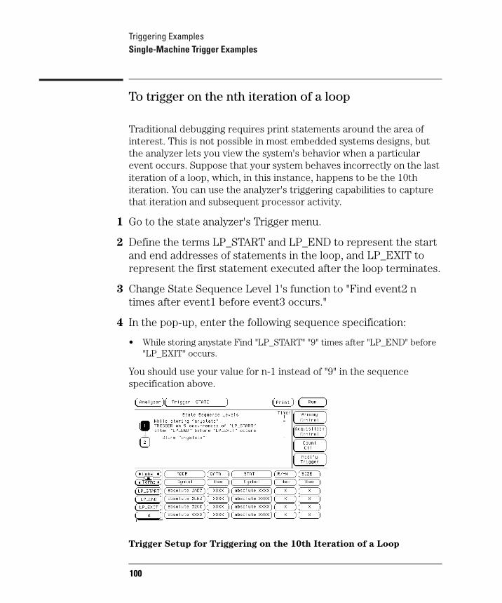
Triggering ExamplesSingle-Machine Trigger Examples
To trigger on the nth iteration of a loop
Traditional debugging requires print statements around the area of interest. This is not possible in most embedded systems designs, but the analyzer lets you view the system's behavior when a particular event occurs. Suppose that your system behaves incorrectly on the last iteration of a loop, which, in this instance, happens to be the 10th iteration. You can use the analyzer's triggering capabilities to capture that iteration and subsequent processor activity.
1 Go to the state analyzer's Trigger menu.
2 Define the terms LP_START and LP_END to represent the start and end addresses of statements in the loop, and LP_EXIT to represent the first statement executed after the loop terminates.
3 Change State Sequence Level 1's function to "Find event2 n times after event1 before event3 occurs."
4 In the pop-up, enter the following sequence specification:
• While storing anystate Find "LP_START" "9" times after "LP_END" before "LP_EXIT" occurs.
You should use your value for n-1 instead of "9" in the sequence specification above.
Trigger Setup for Triggering on the 10th Iteration of a Loop
100
Triggering ExamplesSingle-Machine Trigger Examples
The specification has some advantages and a potential problem.
• The advantages are that a pipelined processor won't trigger until it has executed the loop 10 times. Requiring LP_END to be seen at least once first ensures that the processor actually entered the loop; then, 9 more iterations of LP_START is really the 10th iteration of the loop. Also, no trigger occurs if the loop executes less than 10 times ƒ the analyzer sees LP_EXIT and restarts the trigger sequence.
• The potential problem is that LP_EXIT may be too near LP_END and thus appear on the bus during a prefetch. The analyzer will constantly restart the sequence and will never trigger. The solution to this problem depends on the structure of your code. You may need to experiment with different trigger sequences to find one that captures only the data you want to view.
101
Triggering ExamplesSingle-Machine Trigger Examples
To trigger on the nth recursive call of a recursive function
1 Go to the state analyzer's Trigger menu.
2 Define the terms CALL_ADD, F_START, and F_END to represent the called address of the recursive function, and the start and end addresses of the function. Define F_EXIT to represent the address of the first program statement executed after the original recursive call has terminated.
Typically, CALL_ADD is the address of the code that sets up the activation record on the stack, F_START is the address of the first statement in the function, and F_END is the address of the last instruction of the function, which does not necessarily correspond to the address of the last statement. If the start of the function and the address called by recursive calls are the same, or you are not interested in the function initialization code, you can use F_START for both CALL_ADD and F_START.
3 Change State Sequence Level 1's function to "Find event2 n times after event1 before event3 occurs."
4 In the pop-up, enter the following sequence specification:
• While storing anystate Find "CALL_ADD" "9" times after "F_START" before "F_EXIT" occurs.
You should use your value for n-1 instead of "9" in the specification.
102
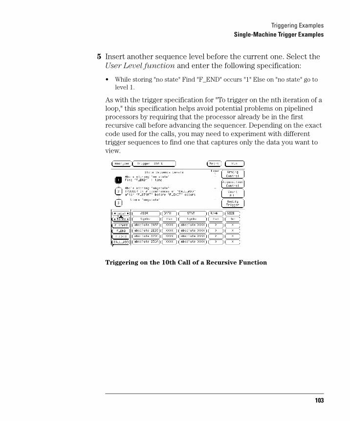
Triggering ExamplesSingle-Machine Trigger Examples
5 Insert another sequence level before the current one. Select the User Level function and enter the following specification:
• While storing "no state" Find "F_END" occurs "1" Else on "no state" go to level 1.
As with the trigger specification for "To trigger on the nth iteration of a loop," this specification helps avoid potential problems on pipelined processors by requiring that the processor already be in the first recursive call before advancing the sequencer. Depending on the exact code used for the calls, you may need to experiment with different trigger sequences to find one that captures only the data you want to view.
Triggering on the 10th Call of a Recursive Function
103

Triggering ExamplesSingle-Machine Trigger Examples
To trigger on entry to a function
This sequence triggers on entry to a function only when it is called by one particular function.
1 Go to the state analyzer's Trigger menu.
2 Define the terms F1_START and F1_END to represent the start and end addresses of the calling function. Define F2_START to represent the start address of the called function.
3 Change State Sequence Level 1's function to "Find event2 n times after event1 before event3 occurs."
4 In the pop-up menu, enter the following sequence specification:
• While storing anystate Find "F2_START" "1" times after "F1_START" before "F1_END" occurs.
This sequence specification assumes there is some conditional logic in function F1 that chooses whether or not to call function F2. Thus, if F1 ends without the analyzer having seen F2, the sequence restarts.
104
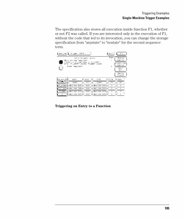
Triggering ExamplesSingle-Machine Trigger Examples
The specification also stores all execution inside function F1, whether or not F2 was called. If you are interested only in the execution of F1, without the code that led to its invocation, you can change the storage specification from "anystate" to "nostate" for the second sequence term.
Triggering on Entry to a Function
105
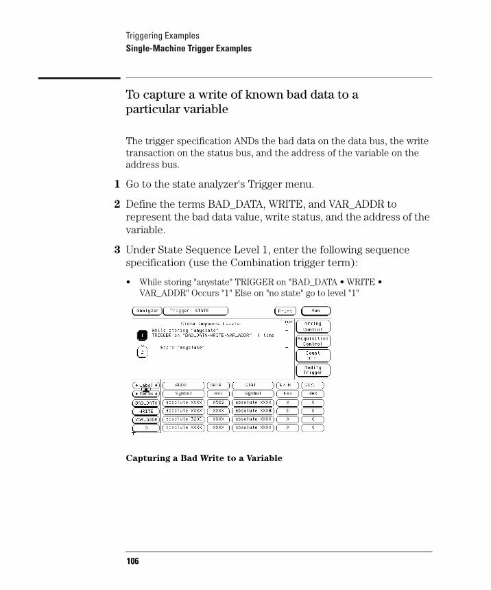
Triggering ExamplesSingle-Machine Trigger Examples
To capture a write of known bad data to a particular variable
The trigger specification ANDs the bad data on the data bus, the write transaction on the status bus, and the address of the variable on the address bus.
1 Go to the state analyzer's Trigger menu.
2 Define the terms BAD_DATA, WRITE, and VAR_ADDR to represent the bad data value, write status, and the address of the variable.
3 Under State Sequence Level 1, enter the following sequence specification (use the Combination trigger term):
• While storing "anystate" TRIGGER on "BAD_DATA • WRITE • VAR_ADDR" Occurs "1" Else on "no state" go to level "1"
Capturing a Bad Write to a Variable
106

Triggering ExamplesSingle-Machine Trigger Examples
To trigger on a loop that occasionally runs too long
This example assumes the loop normally executes in 14 ms.
1 Go to the state analyzer's Trigger menu.
2 Define terms LP_START and LP_END to represent the start and end addresses of the loop, and set Timer1 to the normal duration of the loop.
3 Change State Sequence Level 1's function to "Find event2 occurring too late after event1."
4 In the pop-up menu, enter the following sequence specification:
• While storing anystate Find "LP_END" occurring too late after "LP_START" Use Timer: "Timer1" Time="14 ms"
Of course, you use your normal loop duration in place of "14 ms." The function will automatically start Timer1 for you.
Triggering on a Loop Overrun
107
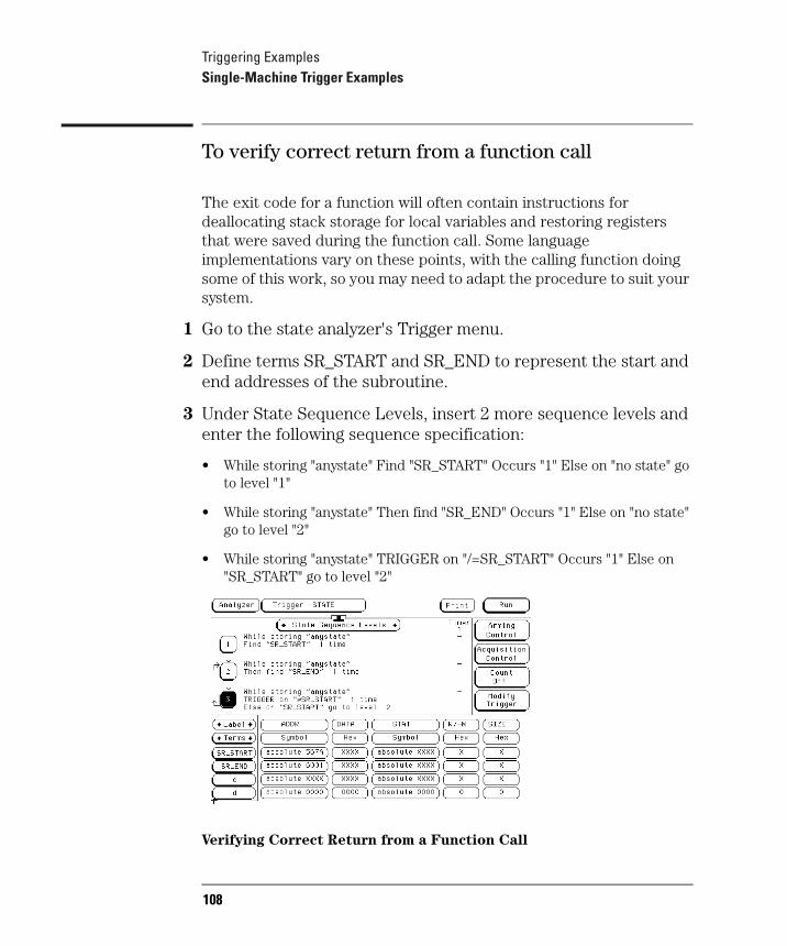
Triggering ExamplesSingle-Machine Trigger Examples
To verify correct return from a function call
The exit code for a function will often contain instructions for deallocating stack storage for local variables and restoring registers that were saved during the function call. Some language implementations vary on these points, with the calling function doing some of this work, so you may need to adapt the procedure to suit your system.
1 Go to the state analyzer's Trigger menu.
2 Define terms SR_START and SR_END to represent the start and end addresses of the subroutine.
3 Under State Sequence Levels, insert 2 more sequence levels and enter the following sequence specification:
• While storing "anystate" Find "SR_START" Occurs "1" Else on "no state" go to level "1"
• While storing "anystate" Then find "SR_END" Occurs "1" Else on "no state" go to level "2"
• While storing "anystate" TRIGGER on "/=SR_START" Occurs "1" Else on "SR_START" go to level "2"
Verifying Correct Return from a Function Call
108
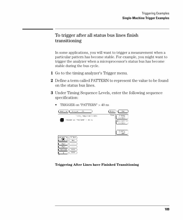
Triggering ExamplesSingle-Machine Trigger Examples
To trigger after all status bus lines finish transitioning
In some applications, you will want to trigger a measurement when a particular pattern has become stable. For example, you might want to trigger the analyzer when a microprocessor's status bus has become stable during the bus cycle.
1 Go to the timing analyzer's Trigger menu.
2 Define a term called PATTERN to represent the value to be found on the status bus lines.
3 Under Timing Sequence Levels, enter the following sequence specification:
• TRIGGER on "PATTERN" > 40 ns
Triggering After Lines have Finished Transitioning
109

Triggering ExamplesSingle-Machine Trigger Examples
To find the nth assertion of a chip select line
1 Go to the timing analyzer's Trigger menu.
2 Define the Edge1 term to represent the asserting transition on the chip select line.
You can rename the Edge1 term to make it correspond more closely to the problem domain, for example, to CHIP_SEL.
3 Under Timing Sequence Levels, enter the following sequence specification:
• TRIGGER on "CHIP_SEL" Occurs "10" Else on "no state" go to level "1"
You should use your value for "n" in place of "10" in the specification above.
Triggering on the 10th Assertion of a Chip Select Line
110
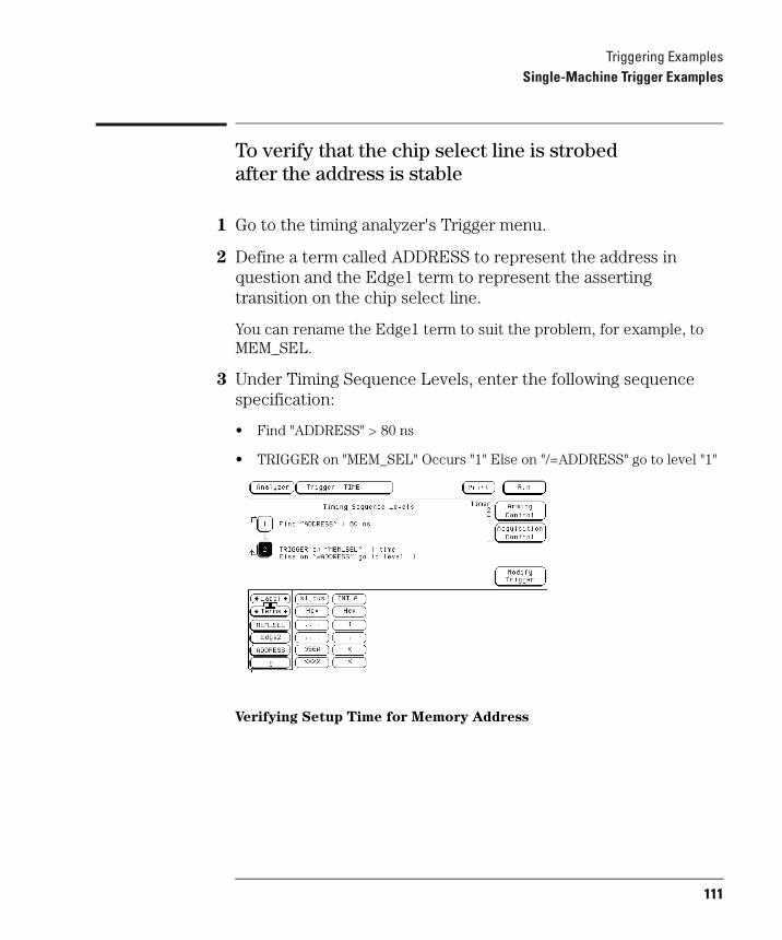
Triggering ExamplesSingle-Machine Trigger Examples
To verify that the chip select line is strobed after the address is stable
1 Go to the timing analyzer's Trigger menu.
2 Define a term called ADDRESS to represent the address in question and the Edge1 term to represent the asserting transition on the chip select line.
You can rename the Edge1 term to suit the problem, for example, to MEM_SEL.
3 Under Timing Sequence Levels, enter the following sequence specification:
• Find "ADDRESS" > 80 ns
• TRIGGER on "MEM_SEL" Occurs "1" Else on "/=ADDRESS" go to level "1"
Verifying Setup Time for Memory Address
111
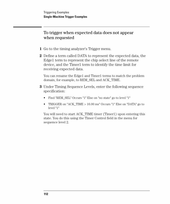
Triggering ExamplesSingle-Machine Trigger Examples
To trigger when expected data does not appear when requested
1 Go to the timing analyzer's Trigger menu.
2 Define a term called DATA to represent the expected data, the Edge1 term to represent the chip select line of the remote device, and the Timer1 term to identify the time limit for receiving expected data.
You can rename the Edge1 and Timer1 terms to match the problem domain, for example, to REM_SEL and ACK_TIME.
3 Under Timing Sequence Levels, enter the following sequence specification:
• Find "REM_SEL" Occurs "1" Else on "no state" go to level "1"
• TRIGGER on "ACK_TIME > 16.00 ms" Occurs "1" Else on "DATA" go to level "1"
You will need to start ACK_TIME timer (Timer1) upon entering this state. You do this using the Timer Control field in the menu for sequence level 2.
112
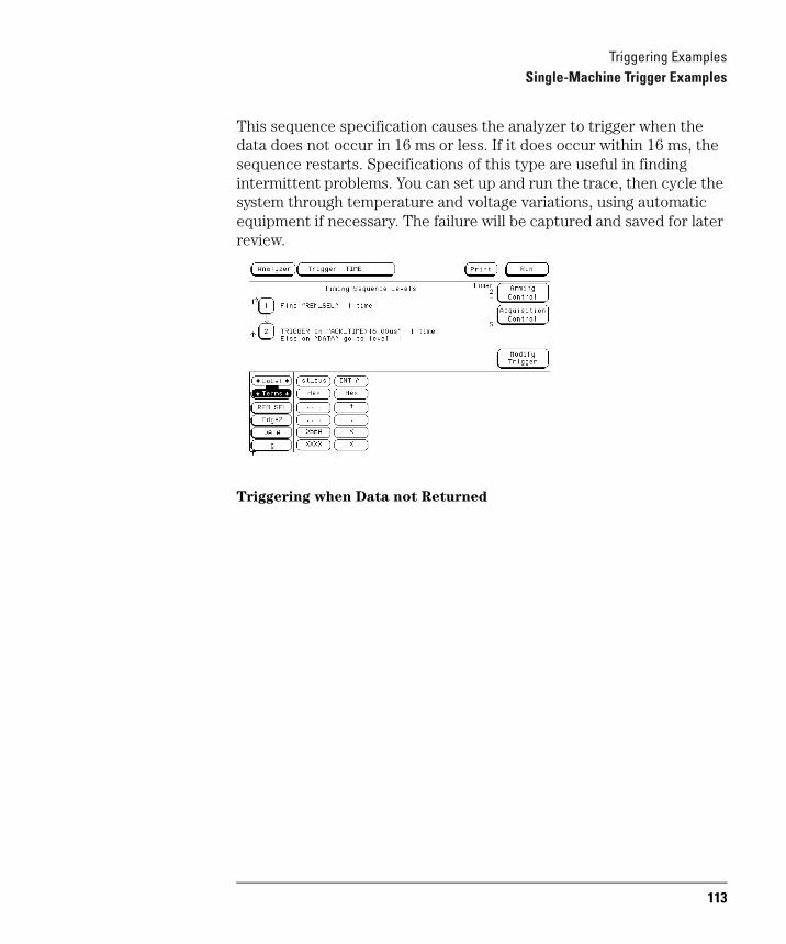
Triggering ExamplesSingle-Machine Trigger Examples
This sequence specification causes the analyzer to trigger when the data does not occur in 16 ms or less. If it does occur within 16 ms, the sequence restarts. Specifications of this type are useful in finding intermittent problems. You can set up and run the trace, then cycle the system through temperature and voltage variations, using automatic equipment if necessary. The failure will be captured and saved for later review.
Triggering when Data not Returned
113
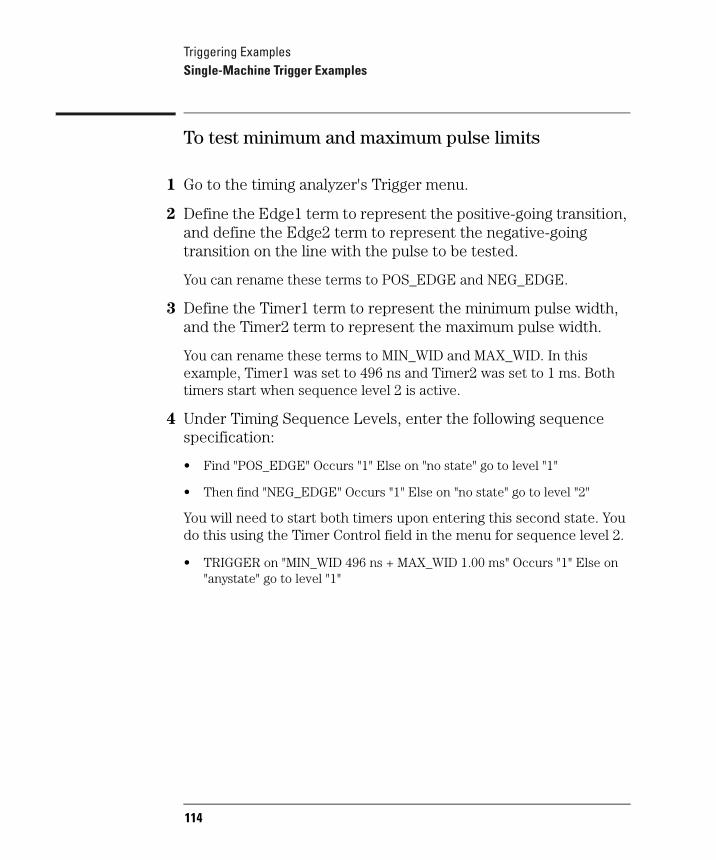
Triggering ExamplesSingle-Machine Trigger Examples
To test minimum and maximum pulse limits
1 Go to the timing analyzer's Trigger menu.
2 Define the Edge1 term to represent the positive-going transition, and define the Edge2 term to represent the negative-going transition on the line with the pulse to be tested.
You can rename these terms to POS_EDGE and NEG_EDGE.
3 Define the Timer1 term to represent the minimum pulse width, and the Timer2 term to represent the maximum pulse width.
You can rename these terms to MIN_WID and MAX_WID. In this example, Timer1 was set to 496 ns and Timer2 was set to 1 ms. Both timers start when sequence level 2 is active.
4 Under Timing Sequence Levels, enter the following sequence specification:
• Find "POS_EDGE" Occurs "1" Else on "no state" go to level "1"
• Then find "NEG_EDGE" Occurs "1" Else on "no state" go to level "2"
You will need to start both timers upon entering this second state. You do this using the Timer Control field in the menu for sequence level 2.
• TRIGGER on "MIN_WID 496 ns + MAX_WID 1.00 ms" Occurs "1" Else on "anystate" go to level "1"
114
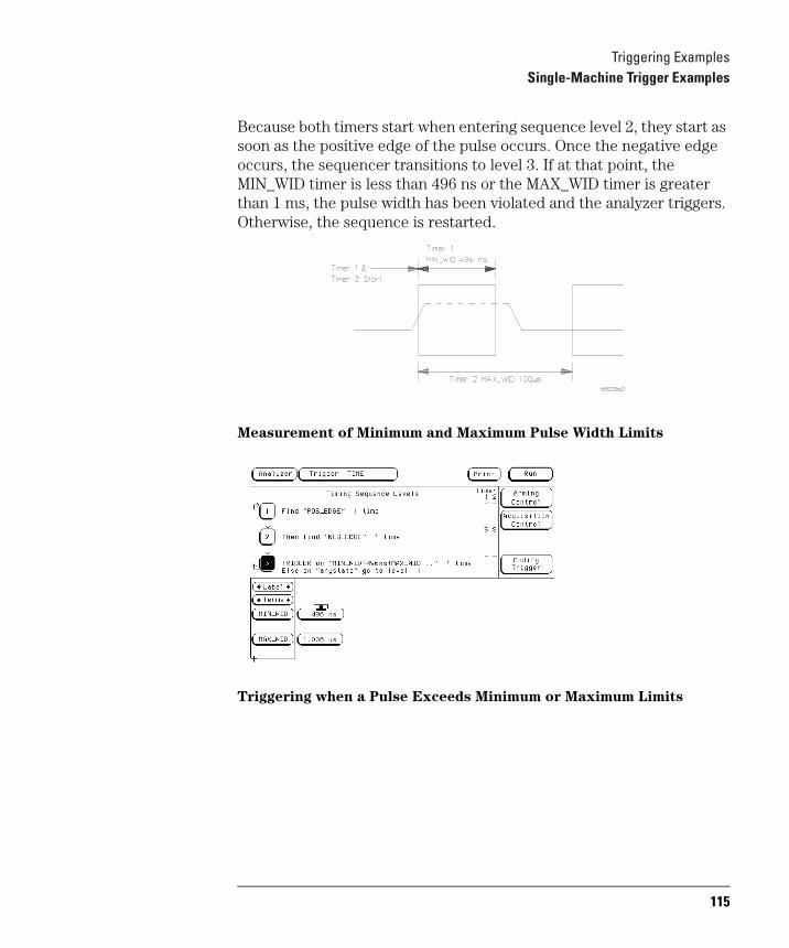
Triggering ExamplesSingle-Machine Trigger Examples
Because both timers start when entering sequence level 2, they start as soon as the positive edge of the pulse occurs. Once the negative edge occurs, the sequencer transitions to level 3. If at that point, the MIN_WID timer is less than 496 ns or the MAX_WID timer is greater than 1 ms, the pulse width has been violated and the analyzer triggers. Otherwise, the sequence is restarted.
Measurement of Minimum and Maximum Pulse Width Limits
Triggering when a Pulse Exceeds Minimum or Maximum Limits
115
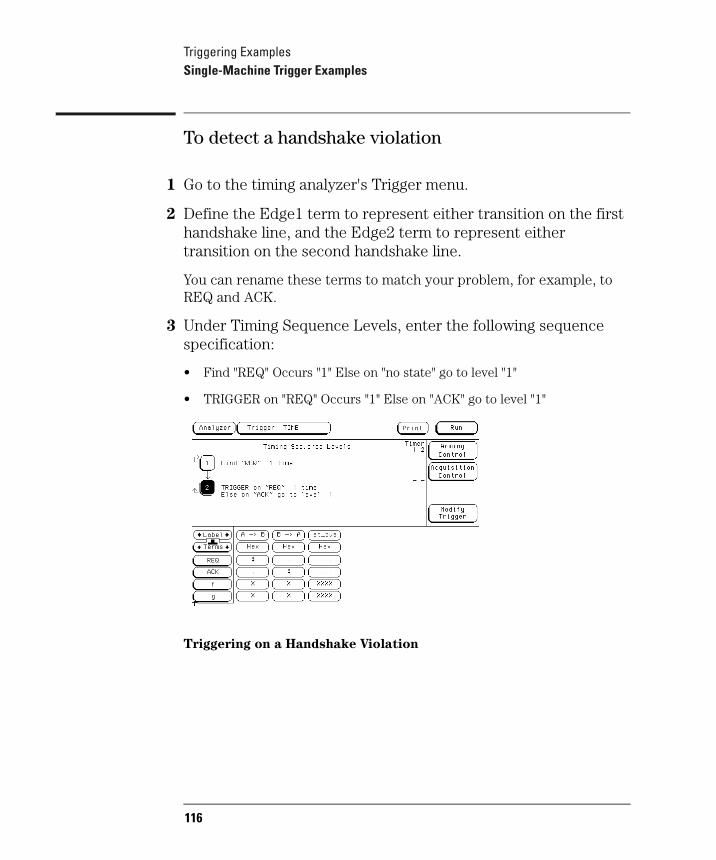
Triggering ExamplesSingle-Machine Trigger Examples
To detect a handshake violation
1 Go to the timing analyzer's Trigger menu.
2 Define the Edge1 term to represent either transition on the first handshake line, and the Edge2 term to represent either transition on the second handshake line.
You can rename these terms to match your problem, for example, to REQ and ACK.
3 Under Timing Sequence Levels, enter the following sequence specification:
• Find "REQ" Occurs "1" Else on "no state" go to level "1"
• TRIGGER on "REQ" Occurs "1" Else on "ACK" go to level "1"
Triggering on a Handshake Violation
116
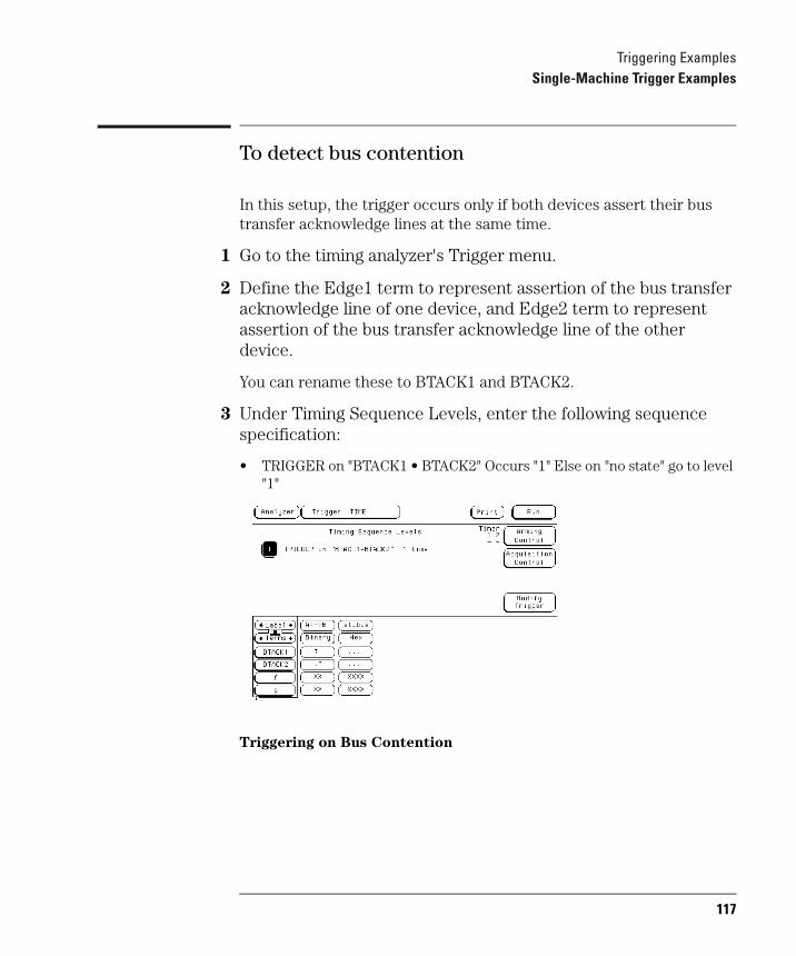
Triggering ExamplesSingle-Machine Trigger Examples
To detect bus contention
In this setup, the trigger occurs only if both devices assert their bus transfer acknowledge lines at the same time.
1 Go to the timing analyzer's Trigger menu.
2 Define the Edge1 term to represent assertion of the bus transfer acknowledge line of one device, and Edge2 term to represent assertion of the bus transfer acknowledge line of the other device.
You can rename these to BTACK1 and BTACK2.
3 Under Timing Sequence Levels, enter the following sequence specification:
• TRIGGER on "BTACK1 • BTACK2" Occurs "1" Else on "no state" go to level "1"
Triggering on Bus Contention
117
Triggering ExamplesCross-Arming Trigger Examples
Cross-Arming Trigger ExamplesThe following examples use cross arming to coordinate measurements between two separate analyzers within the logic analyzer or between analyzers and the oscilloscope. The analyzers can be configured as either a state analyzer and timing analyzer, or two state analyzers. It is not possible to set both to timing.
You set up cross arming in the Arming Control menu (obtained by selecting Arming Control in the Trigger menu). When coordinating measurements between two instruments, you need to select Count Time to correlate the measurements. When correlating measurements between an analyzer and the oscilloscope you also need to set the oscilloscope Trigger Mode to Immediate.
118
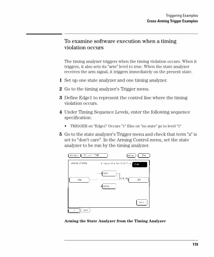
Triggering ExamplesCross-Arming Trigger Examples
To examine software execution when a timing violation occurs
The timing analyzer triggers when the timing violation occurs. When it triggers, it also sets its "arm" level to true. When the state analyzer receives the arm signal, it triggers immediately on the present state.
1 Set up one state analyzer and one timing analyzer.
2 Go to the timing analyzer's Trigger menu.
3 Define Edge1 to represent the control line where the timing violation occurs.
4 Under Timing Sequence Levels, enter the following sequence specification:
• TRIGGER on "Edge1" Occurs "1" Else on "no state" go to level "1"
5 Go to the state analyzer's Trigger menu and check that term "a" is set to "don't care". In the Arming Control menu, set the state analyzer to be run by the timing analyzer.
Arming the State Analyzer from the Timing Analyzer
119
Triggering ExamplesCross-Arming Trigger Examples
6 Under State Sequence Levels, enter the following sequence specification:
• While storing "anystate" TRIGGER on "arm a" Occurs "1" Else on "no state" go to level "1"
120

Triggering ExamplesCross-Arming Trigger Examples
To look at control and status signals during execution of a routine
The state analyzer will trigger on the start of the routine whose control and status signals are to be examined more frequently than once per bus cycle. When the state analyzer triggers, it sends out an arm signal. The timing analyzer triggers when it receives the true arm level and detects the transition represented by Edge1.
1 Set up one state analyzer and one timing analyzer.
2 Go to the state analyzer's Trigger menu and define term R_START to represent the starting address of the routine.
3 Under State Sequence Levels, enter the following sequence specification:
• While storing "anystate" TRIGGER on "R_START" Occurs "1" Else on "no state" go to level "1"
4 Go to the timing analyzer's Trigger menu.
5 Define the Edge1 term to represent a transition on one of the control signals.
6 Set the timing analyzer to be run by the state analyzer. Under Timing Sequence Levels, enter the following sequence specification:
• TRIGGER on "arm Edge1" 1 time
You do not need to use a combination trigger when one analyzer is armed from the other analyzer - the arm term is ANDed automatically with the term already in use at that level.
121
Triggering ExamplesCross-Arming Trigger Examples
To detect a glitch
The following setup uses a state analyzer to capture state flow occurring at the time of the glitch. This can be useful in troubleshooting. For example, you might find that the glitch is ground bounce caused by a number of simultaneous signal transitions.
1 Set up a timing analyzer and a state analyzer.
2 Go to the timing analyzer's Format menu and set the Timing Acquisition Mode to Half Channel 500 MHz.
3 Go to the timing analyzer's Trigger menu.
4 Select an Edge term. Then assign glitch detection "*" to the channels of interest represented by the Edge term.
5 Go to the state analyzer's Trigger menu.
6 Set the analyzer to be armed by the timing analyzer. Leave the trigger set to trigger on any state.
If you don't see the activity of interest in the state trace, try changing the trigger position using the Acquisition Control field in the Trigger menu of the state analyzer. By changing the Acquisition mode to manual, you can position the trigger at any state relative to analyzer memory.
NOTE: The timing analyzer can detect glitch activity on a waveform. A glitch is defined as two or more transitions across the logic threshold between adjacent timing analyzer samples.
122
Triggering ExamplesCross-Arming Trigger Examples
To capture the waveform of a glitch using the oscilloscope (oscilloscope option only)
The following setup uses the triggering capability of the timing analyzer and the acquisition capability of the oscilloscope.
1 Set up a timing analyzer. Go to the timing analyzer’s Format menu and set the Timing Acquisition Mode to Half Channel 500 MHz.
2 Go to the timing analyzer’s Trigger menu.
3 Select an Edge term. Then assign glitch detection “*” to the channels of interest represented by the Edge term.
4 Go to the Arming Control menu. Set the Scope Arm In to Analyzer.
5 Select Group Run in the Analyzer Arm In menu.
6 Go to the Scope Trigger menu, and set Mode to Immediate.
If you have trouble capturing the glitch waveform on the oscilloscope, try adjusting the skew in the Arming Control menu, so the oscilloscope triggers earlier.
NOTE: A timing analyzer can trigger on a glitch and capture it, but a timing analyzer doesn’t have the voltage or timing resolution to display the glitch in detail. An oscilloscope can display a glitch waveform with fine resolution, but cannot trigger on glitches, combinations of glitches, or sophisticated patterns involving many channels.
123
Triggering ExamplesCross-Arming Trigger Examples
To view your target system processing an interrupt (oscilloscope option only)
Use the oscilloscope to trigger on the asynchronous interrupt request.
1 Go to the state analyzer’s Trigger menu, and set the analyzer to trigger on any state and store any state.
2 Select Arming Control. Set the analyzer to respond to the arm signal from the oscilloscope, and set the oscilloscope to Group
Run.
3 Go to the Scope Trigger menu, and set the mode to Edge trigger. Set the Source field to C1, and probe the interrupt with Channel 1.
4 Press the Run key.
When the interrupt occurs, the oscilloscope will trigger, subsequently triggering the state analyzer.
If the analyzer doesn’t capture the expected interrupt activity, ensure that the interrupt isn’t masked due to the actions of other program code.
This setup can help you answer questions like the following:
• Does the processor branch to the proper interrupt handling routine?• Are registers and status information saved properly?• How long does it take to service the interrupt?• Is the interrupt acknowledged properly?• After the interrupt is serviced, does the processor restore registers and
status information and continue with the interrupted routine as expected?
You can use the state analyzer to check the address of the interrupt routine as well as to see if interrupt processing is done as expected. Using an analysis probe and inverse assembler with the state analyzer will make it easier to read the program flow.
124
Triggering ExamplesCross-Arming Trigger Examples
To trigger timing analysis of a count-down on a set of data lines
Your target system may include various state machines that are started by system events such as interrupt processing or I/O activity. The state analyzer is ideal for recognizing the system events; the timing analyzer is ideal for examining the step-by-step operation of the state machines.
1 Set up a timing analyzer and a state analyzer.
2 Go to the state analyzer's Trigger menu.
3 Set the timing analyzer to be run from the state analyzer.
4 Set the state analyzer to trigger on the label and term that identify the start of the count-down routine.
5 Go to the timing analyzer's Trigger Menu.
6 Set the timing analyzer to trigger on any state and store any state.
125

Triggering ExamplesCross-Arming Trigger Examples
To monitor two coprocessors in a target system
Debugging coprocessor systems can be a complex task. Replicated systems and contention for shared resources increase the potential problems. Using two state analyzers with analysis probes can make it much easier to discover the source of such problems. For example, you may want to set up one analyzer to trigger only when a certain problem occurs, and set up the other analyzer to be armed by the first analyzer so that it takes its trace only when the first analyzer recognizes its trigger. This will let you observe the behavior of both coprocessors during the occurrence of a problem.
1 Set up both analyzers as state analyzers.
2 Go to the first analyzer's Trigger menu.
3 Set the second analyzer to be run from the first analyzer.
4 Turn on Count Time.
5 Set the first analyzer to trigger on the problem condition.
Some problems may involve complex sequences of conditions. See earlier examples in this chapter for more information on defining trigger sequences.
6 Go to the Trigger menu of the second analyzer.
126
Triggering ExamplesCross-Arming Trigger Examples
7 Check that the second analyzer is triggering on arm and that Count Time is set.
After the measurement is complete, you can interleave the trace lists of both state analyzers to see the activity executed by both coprocessors during related clock cycles.
You can use a similar procedure if you have only one processor, but want to monitor its activity with that of other system nodes, such as chip-select lines, I/O activity, or behavior of a watchdog timer. In some instances it may be easier to look at related activity with a timing analyzer.
See Also "Special Displays" on page 128.
"To trigger timing analysis of a count-down on a set of data lines" on page 125.
127
Triggering ExamplesSpecial Displays
Special Displays
Interleaved trace lists
Interleaved trace lists allow you to view data captured by two analyzers in a single display. When you interleave the traces, you see each state that was captured by each analyzer. These states are shown on consecutive lines.
You can interleave state listings from state analyzers when two are used together in a run. Interleaved state listings are useful when you are using multiple analyzers to look at interaction between two or more processors. They are also useful when you need more analysis width than is available in one analyzer.
Mixed Display mode
The Mixed Display mode allows you to show state listings and timing waveforms together on screen. State listings are shown at the top of the screen and waveform displays are shown at the bottom. You can interleave state listings from two analyzers at the top of the screen, if desired. You can display waveforms from the timing analyzer at the bottom of the screen.
128
Triggering ExamplesSpecial Displays
To interleave trace lists
1 Set up both analyzers as state analyzers.
2 Go to the Trigger menu of the first analyzer.
3 Set Count to Time, and set up the trigger.
The logic analyzer uses the time tags stored with each state to determine the ordering of states shown in an interleaved trace list.
4 Set Count to Time, and set up the trigger on the second analyzer.
The second analyzer does not need to be run from the first analyzer, but both analyzers must have "Count Time" turned on to correlate the data.
5 Make the measurement run.
6 Go to one of the Listing menus.
7 Select one of the label fields in the trace list display, then select Interleave.
129
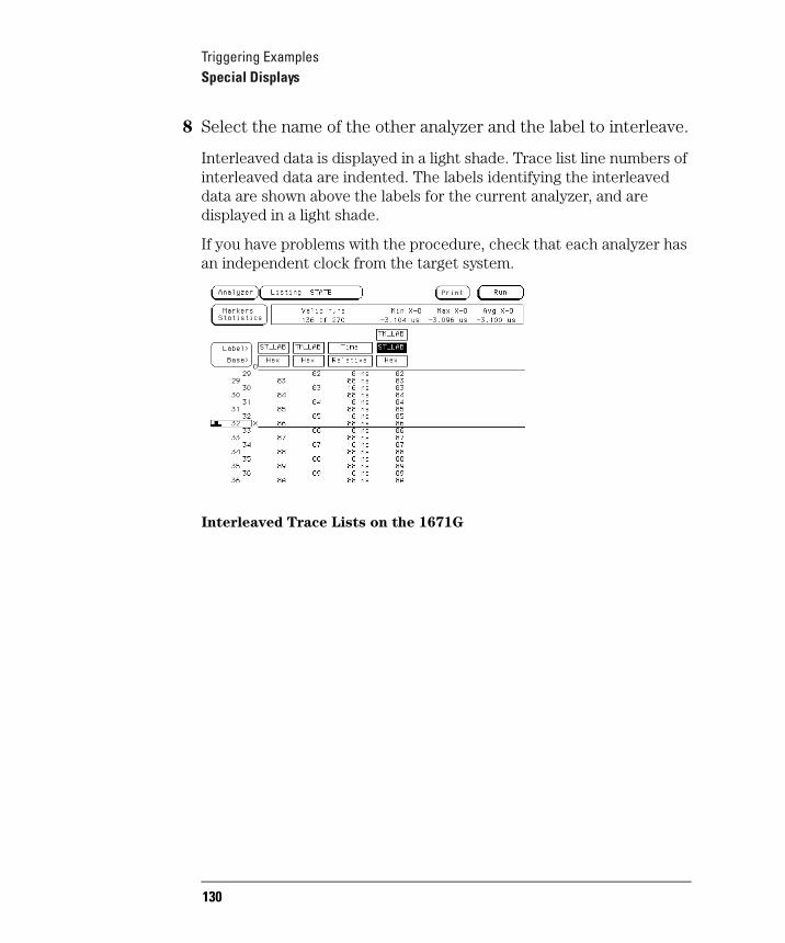
Triggering ExamplesSpecial Displays
8 Select the name of the other analyzer and the label to interleave.
Interleaved data is displayed in a light shade. Trace list line numbers of interleaved data are indented. The labels identifying the interleaved data are shown above the labels for the current analyzer, and are displayed in a light shade.
If you have problems with the procedure, check that each analyzer has an independent clock from the target system.
Interleaved Trace Lists on the 1671G
130

Triggering ExamplesSpecial Displays
To view trace lists and waveforms on the same display
1 Set up a timing and a state analyzer.
2 Go to the state analyzer's Trigger menu.
3 Set Count to Time, and set up the trigger as appropriate.
You do not need to have one instrument arming the other to display the information jointly, but you do need to turn on Count Time so that the information may be correlated.
4 Set up the timing analyzer trigger.
Timing analyzers implicitly count time because their sampling is driven by an internal clock, rather than an external state clock.
5 Make a measurement run.
6 Go to the Mixed Display menu.
7 To insert state listings, select any label field from the state listing. From the pop-up that appears, select the desired label to insert.
8 To insert timing or waveforms, double-select the label field to the left of the waveform display area. From the pop-up that appears, select insert, and then the appropriate label.
131

Triggering ExamplesSpecial Displays
You cannot view state analyzer data in the waveform display. However, you can view timing analyzer data and oscilloscope data simultaneously.
You can also position X and O Time markers on the waveform display. Once set, the time markers will be displayed in both the listing and the waveform display areas. Note that even if you set X and O Time markers in another display, you must also set the Time markers in the Mixed Display if Time markers are desired.
NOTE: You can use the Mixed Display feature in the analyzer menu to show both waveforms and trace lists in the same display, making it easier to correlate the events of interest.
Mixed Display using Timing and State in the 1671G
132

6
File Management
133
File ManagementFile Management
File ManagementBeing able to transfer data to a host computer, such as a PC or UNIX workstation, can enhance the logic analyzer in many ways. You can use the host to store configuration files or measurement results for later review. You can save screen images from the logic analyzer in bitmap files to include in reports developed using word processors or desktop publishing tools. Or, you can develop programs on the PC that manipulate measurement results to satisfy your problem-solving needs.
This chapter shows you how to save the different types of information. The examples store files on the flexible disk drive, but you can move the same files to your host computer using a network interface. The 1670G-series of logic analyzers have GPIB and RS-232-C capabilities, and an ethernet interface. If you need help using the LAN interface, see the LAN section of this book on page 476.
You can also use a host computer to send the logic analyzer complex command sequences allowing you to automate your measurement tasks. If you want to program the analyzer using a host computer, see the Agilent Technologies 1670G-Series Logic Analyzers Programmer's Guide.
134
File ManagementTransferring Files Using the Flexible Disk Drive
Transferring Files Using the Flexible Disk DriveBecause the flexible disk drive on the 1670G-series logic analyzers will read and write double-sided, double-density, or high-density disks in MS-DOS format, it is a useful tool for transferring data to and from IBM PC-compatible computers as well as transferring data to and from other systems that can read and write MS-DOS format. You can save configuration files, measurement results, and even menu and measurement images from the screen.
This section shows you how to use the flexible disk drive to:
• Save a configuration
• Load a configuration
• Save a trace list in ASCII format
• Save a screen image (such as a display or menu)
• Load additional software
135
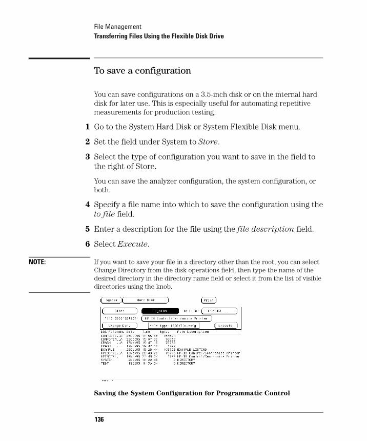
File ManagementTransferring Files Using the Flexible Disk Drive
To save a configuration
You can save configurations on a 3.5-inch disk or on the internal hard disk for later use. This is especially useful for automating repetitive measurements for production testing.
1 Go to the System Hard Disk or System Flexible Disk menu.
2 Set the field under System to Store.
3 Select the type of configuration you want to save in the field to the right of Store.
You can save the analyzer configuration, the system configuration, or both.
4 Specify a file name into which to save the configuration using theto file field.
5 Enter a description for the file using the file description field.
6 Select Execute.
NOTE: If you want to save your file in a directory other than the root, you can select Change Directory from the disk operations field, then type the name of the desired directory in the directory name field or select it from the list of visible directories using the knob.
Saving the System Configuration for Programmatic Control
136

File ManagementTransferring Files Using the Flexible Disk Drive
To load a configuration
You can quickly load a previously saved configuration, so that you will not have to manually set up the measurement parameters.
1 Go to the System Hard Disk or System Flexible Disk menu.
Your choice here depends on where you saved the configuration.
2 Select the field below System and select Load from the pop-up menu.
3 Select the destination from the module list.
"System" loads only settings available under the System menus. "Analyzer" loads data and settings for the analyzer. "All" loads both the system and analyzer configurations.
You can only load configuration files to the area from which the configuration was taken. For instance, you cannot load an analyzer configuration file to the system. Thus, if you select System, then select a file that contains only an analyzer configuration, the configuration will fail. The file type field tells you what type of information is in a file. Analyzer configuration files show “167xan_config”, and system configurations show "167x_cnfg" in the file type field.
4 Specify a file name from which to load the configuration using the from file field or scrolling with the knob.
137

File ManagementTransferring Files Using the Flexible Disk Drive
5 Select Execute.
Loading System Configuration for Programmatic Control
138

File ManagementTransferring Files Using the Flexible Disk Drive
To save a trace list in ASCII format
Some screens, such as file lists and trace lists, contain columns of ASCII data that you may want to move to a computer for further manipulation or analysis. You can save these displays as ASCII files. While a screen capture saves only the data shown onscreen, saving the display as an ASCII file captures all data in the list, even if it is offscreen.
1 Insert a DOS-formatted 3.5-inch disk in the flexible disk drive.
2 Set up the menu you want to capture, or run a measurement from which you want to save data.
Remember that only displays that present lists of textual data can be captured as ASCII files.
3 Select Print and choose Print Disk from the pop-up menu.
4 Select the Filename field and specify a file name to which the data will be saved.
5 Select ASCII (ALL) from the Output Format field.
If the current display contents can not be saved as an ASCII file, this option will not be present in the Output Format field.
6 Select Flexible Disk from the Output Disk menu, then select Execute.
139
File ManagementTransferring Files Using the Flexible Disk Drive
To save a screen's image
You can save menus and measurements to disk in one of four different graphical formats.
1 Insert a formatted flexible disk in the flexible disk drive.
2 Set up the menu whose image you want to capture, or run a measurement from which you want to save data.
3 Select Print and choose Print Disk from the pop-up menu.
If the screen contains a pop-up menu, the Print field is not available. Pop-up menus cannot be saved to file unless you are using a controller.
4 Select the Filename field and specify a file name to save to.
5 Select the Output Format field and choose the output format for the graphics file from the pop-up menu.
• Choose one of the following formats:
• B/W TIF is a black-and-white TIFF (Tagged Image File Format), v 5.0.
• COLOR TIF is a color TIFF file in TIFF version 5.0 format.
• PCX is a color PCX file (PCX is the PC Paintbrush and Publisher's Paintbrush format from ZSoft).
• EPS is a black-and-white Encapsulated PostScriptø file.
140
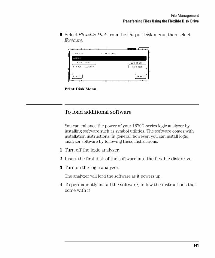
File ManagementTransferring Files Using the Flexible Disk Drive
6 Select Flexible Disk from the Output Disk menu, then select Execute.
Print Disk Menu
To load additional software
You can enhance the power of your 1670G-series logic analyzer by installing software such as symbol utilities. The software comes with installation instructions. In general, however, you can install logic analyzer software by following these instructions.
1 Turn off the logic analyzer.
2 Insert the first disk of the software into the flexible disk drive.
3 Turn on the logic analyzer.
The analyzer will load the software as it powers up.
4 To permanently install the software, follow the instructions that come with it.
141
File ManagementTransferring Files Using the LAN
Transferring Files Using the LANThe 1670G-series logic analyzers come equipped with a LAN interface. You can transfer information from the logic analyzer to a computer for processing or storage over the LAN without ever copying a file to disk.
Because there are so many different network software packages, this section does not attempt to explain how to put your logic analyzer on the local network or how to establish a network connection. Those topics are covered in detail and with many examples in the LAN Section of this User’s Guide.
There are three basic types of connection you can establish between a computer and the logic analyzer over an Ethernet LAN: ftp, telnet, and X Window. ftp (File Transfer Protocol) is a common UNIX® program for copying files between two computers. It is also available on many PCs. A telnet or X Window connection is better suited than ftp for controlling the logic analyzer, but they cannot transfer files.
See Also The LAN section of this User’s Guide on page 476 for more information on setting up connections.
142

File ManagementTransferring Files Using the LAN
To transfer files using ftp
1 Check that your network package include ftp, and connect your logic analyzer to the LAN.
See the LAN section of this User’s Guide on page 476 for instructions.
2 From the computer you want to transfer the files to or from, establish an ftp connection.
3 At the login prompt, log in as data or control.
If you want to load files into the logic analyzer, log in as control. Otherwise, log in as data.
4 If you will be transferring screen images or configuration files, set type to BIN.
5 Locate the file you want, and transfer it.
“The File System” on page 387 explains the different types of files in the file system. Most ftp software lets you use your regular computer commands for moving around the remote file system and listing files. To copy files, most ftp software uses get and put.
143

File ManagementTransferring Files Using the LAN
144
7
Using the Oscilloscope
145

Using the OscilloscopeUsing the Oscilloscope
Using the OscilloscopeThis chapter covers the oscilloscope common menus and calibration. This chapter covers:
• calibrating the oscilloscope
• oscilloscope common menus.
The oscilloscope circuitry requires an operational accuracy calibration by the user or service department under any of the following conditions:
• at six month intervals or every 1000 hours
• if ambient temperature changes more than 10°C from the temperature at full calibration
• to optimize measurement accuracy.
To test the oscilloscope circuitry against specifications (full calibration), refer to chapter 3, Testing Performance in the “Agilent Technologies 1670G-Series Logic Analyzers Service Guide.”
146

Using the OscilloscopeCalibrating the oscilloscope
Calibrating the oscilloscope
Equipment Required
Calibration PROTECT/UNPROTECT switch
The 1670G-series logic analyzers have a calibration PROTECT/UNPROTECT switch on the back panel. This switch must be set to UNPROTECT before new calibration values from the operational accuracy calibration can be stored to nonvolatile RAM.
Set up the equipment
1 Turn on the logic analyzer. Let it warm up for 30 minutes if you have not already done so.
2 Facing the front panel, reach around to the lower right corner on the back of the logic analyzer. Flip the PROTECT/UNPROTECT switch to UNPROTECT (flip the switch up).
Equipment Critical Specification Recommended Agilent Model/Part Qty
Cable (2) BNC, 9-inch (equal length) 10502A 1
Cable 50 W BNC (m-to-m) 48-inch 10503A 1
Adapter BNC tee (m)(f)(f) 1250-0781 1
Adapter BNC (f)(f) (ug-914/u) 1250-0080 1
147
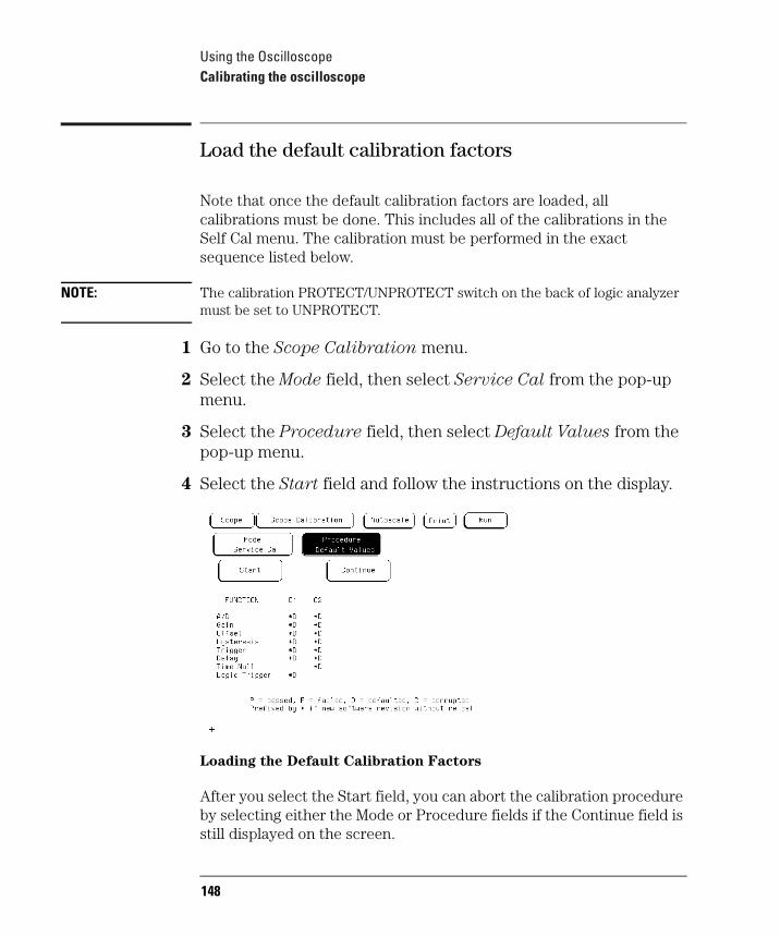
Using the OscilloscopeCalibrating the oscilloscope
Load the default calibration factors
Note that once the default calibration factors are loaded, all calibrations must be done. This includes all of the calibrations in the Self Cal menu. The calibration must be performed in the exact sequence listed below.
NOTE: The calibration PROTECT/UNPROTECT switch on the back of logic analyzer must be set to UNPROTECT.
1 Go to the Scope Calibration menu.
2 Select the Mode field, then select Service Cal from the pop-up menu.
3 Select the Procedure field, then select Default Values from the pop-up menu.
4 Select the Start field and follow the instructions on the display.
Loading the Default Calibration Factors
After you select the Start field, you can abort the calibration procedure by selecting either the Mode or Procedure fields if the Continue field is still displayed on the screen.
148
Using the OscilloscopeCalibrating the oscilloscope
Self Cal menu calibrations
Messages will be displayed as each calibration routine is completed to indicate calibration has passed or failed. The resulting calibration factors are automatically stored to nonvolatile RAM at the conclusion of each calibration routine.
The Self Cal menu lets you optimize vertical sensitivity (Vert Cal) for channels 1 and 2 individually or both channels on a board simultaneously. Also, the Self Cal menu lets you optimize delay (Delay) for channel 1 and 2 separately, then Time Null for channel 2 and the Logic Trigger.
1 Optimize Vert Cal of the Self Cal.
a Connect two BNC 50-W, 9-inch cables to the BNC tee adapter. Connect the BNC 50W (f)(f) adapter to the BNC tee adapter, and connect the 48-inch BNC cable to the BNC 50W (f)(f) adapter. Once you select Start, the instrument will prompt you to connect the cables to the appropriate locations on the rear panel of the instrument.
b Select the Mode field, then select Self Cal from the pop-up menu.
c Select the Procedure field, then select Vert Cal from the pop-up menu.
d Select the Channel field, then select a channel choice from the pop-up menu.
e Select the Start field and follow the instructions on the display.
f After completion of Vertical Calibration, remove the cables from the instrument.
149
Using the OscilloscopeCalibrating the oscilloscope
2 Optimize Delay of the Self Cal.
a Obtain a BNC 50-W, 48-inch cable. Once you select Start, the instrument will prompt you to connect the cable to the appropriate location on the rear panel of the instrument.
b Select the Procedure field, then select Delay from the pop-up menu.
c Select the Channel field, then select C1.
d Select the Start field and follow the instructions on the display.
e Repeat steps c and d for channel 2.
f After completing all of the channel delay calibrations, remove the cable from the oscilloscope.
3 Optimize the Time Null of the Self Cal.
a Connect two BNC 50-W, 9-inch cables to the BNC tee adapter. Connect the BNC 50W (f)(f) adapter to the BNC tee adapter, and connect the 48-inch BNC cable to the BNC 50W (f)(f) adapter. Once you select Start, the instrument will prompt you to connect the cables to the appropriate locations on the rear panel of the instrument.
b Select the Procedure field, then select Time Null from the pop-up menu.
c Select the Start field and follow the instructions on the display.
d After completion of the Time Null calibration, remove the cables from the instrument.
150
Using the OscilloscopeCalibrating the oscilloscope
4 Calibrate the Logic Trigger of the Self Cal.
a Obtain a BNC 50-W, 48-inch cable.
b Select Start. The instrument will prompt you to connect the cable to the appropriate location on the rear panel of the instrument.
c Select the Procedure field, then select Logic Trigger from the pop-up menu.
d Select the Start field and follow the instructions on the display.
e After completion of the Logic Trigger calibration, remove the cable from the instrument.
Protect the operational accuracy calibration factors
• Facing the front panel, reach around to the lower right corner on the back of the logic analyzer. Flip the PROTECT/UNPROTECT switch to PROTECT (flip the switch down).
151
Using the OscilloscopeOscilloscope Common Menus
Oscilloscope Common MenusThe following options apply to all of the oscilloscope menus.
Run/Stop options
There are three ways you can manually run and stop the oscilloscope: the Autoscale menu, the Run and Stop keys, and the Run/Stop field.
Single and Repetitive modes
Single mode acquisition fills acquisition memory once with 8000 samples of the input waveform, automatically stops running, then displays the contents of acquisition memory. Each 8000-sample waveform record is acquired in a single acquisition. Each channel has a memory capacity of 8000 samples.
Repetitive mode acquisition fills acquisition memory with 8000 samples of the input waveform on continuing acquisitions, with each new acquisition overwriting the previous. The display is updated each time a new acquisition is made. Repetitive mode continues acquiring data in this manner until you select the Stop field. As in single mode, each 8000-sample waveform record is acquired in a single acquisition.
Autoscale run
Select the autoscale field on the screen, then choose Continue from the pop-up menu. When autoscaling is complete, the oscilloscope automatically starts running.
152
Using the OscilloscopeOscilloscope Common Menus
If you have been using the Run field to initiate your runs, the oscilloscope will run in the mode (single or repetitive) that was last chosen using the Run options. If no run mode has been chosen prior to choosing autoscale, the run mode defaults to single mode.
If you have been using the Run key to initiate your runs, the oscilloscope will run in single mode.
See Also "Autoscale" on page 154 for information on how the autoscale algorithm works.
153
Using the OscilloscopeOscilloscope Common Menus
Autoscale
Autoscale is an algorithm that automatically optimizes the display of one or more waveforms. When you select the Autoscale field and choose Continue, the autoscale algorithm starts.
What the Autoscale algorithm does when a signal is found
The autoscale algorithm first checks all input channels to determine whether or not there are any signals present. The vertical scaling is then set as required for each channel. Next the time base is scaled for a single input channel, the trigger channel is selected, the data is acquired, and the waveforms are displayed.
Finding the vertical settings. The autoscale algorithm sets the vertical scaling (V/Div and offset) appropriate to the input signal for channel 1. This process is repeated for channel 2.
Finding the time base settings. The time base settings (s/Div and delay) are determined based on the input signal of Channel 1 (if active) or Channel 2. The time base is scaled so that between two and five complete cycles of the time base scaling source input signal can be seen on the screen. The trigger settings are also changed by the autoscale algorithm and an edge mode trigger with CHAN 1 or CHAN 2 is selected. The channel selected for time base scaling is selected as the trigger source.
154
Using the OscilloscopeOscilloscope Common Menus
Displaying the waveform. When the autoscale algorithm is complete, the oscilloscope automatically starts running, acquires the data, and displays waveforms for the inputs that have been selected.
The trigger point on the waveform is determined by the trigger level set by the autoscale algorithm. The trigger point is displayed as a dotted vertical line at the center of the screen (Delay = 0 s).
What the Autoscale algorithm does when a signal is not found .
If no signal is found, the autoscale algorithm toggles the Auto-Trig field to On, which places the oscilloscope in the automatic trigger mode. The oscilloscope then displays the message "Auto triggered." The automatic trigger mode allows the oscilloscope to sweep automatically and to display a baseline anytime a trigger signal is not present. All other settings are restored to their original values.
Menus and fields changed by the Autoscale algorithm
The following table shows the menus and their fields that are changed by the autoscale algorithm.
Settings Changed by Autoscale
Menu Field AutoscaleChannel V/Div
OffsetScaled - depending on amplitude of input signal.Scaled - depending on offset of input signal.
Trigger ModeSourceLevelSlopeCountAuto-Trig
Defaults to Edge.Set to lowest numbered channel with signal present.Scaled - depending on amplitude of lowest numbered channel with signal present.Defaults to Positive.Defaults to 1.Defaults to On.
All Applicable
s/DivDelay
Scaled - depending on frequency of lowest numbered channel with signal present.Defaults to 0 s.
155
Using the OscilloscopeOscilloscope Common Menus
Time base
The s/Div and Delay fields are displayed on all of the oscilloscope menus, except for the Calibration menu.
s/Div field
The s/Div field allows you to set the sweep speed (time scale) on the horizontal axis of the display from 500 ps/div to 5 sec/div. Sweep speed is measured in seconds per division.
Delay field
The Delay field allows you to set the horizontal position of the displayed waveform in relation to the trigger. Delay time is always measured from the trigger point on the waveform to the center of the screen. Delay time is measured in seconds. When acquisitions are stopped, the Delay field can be used to control the portion of acquisition memory displayed on screen.
156
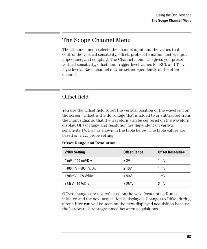
Using the OscilloscopeThe Scope Channel Menu
The Scope Channel MenuThe Channel menu selects the channel input and the values that control the vertical sensitivity, offset, probe attenuation factor, input impedance, and coupling. The Channel menu also gives you preset vertical sensitivity, offset, and trigger level values for ECL and TTL logic levels. Each channel may be set independently of the other channel.
Offset field
You use the Offset field to set the vertical position of the waveform on the screen. Offset is the dc voltage that is added to or subtracted from the input signal so that the waveform can be centered on the waveform display. Offset range and resolution are dependent on vertical sensitivity (V/Div) as shown in the table below. The table values are based on a 1:1 probe setting.
Offset Range and Resolution
Offset changes are not reflected on the waveform until a Run is initiated and the next acquisition is displayed. Changes to Offset during a repetitive run will be seen on the next displayed acquisition because the hardware is reprogrammed between acquisitions.
V/Div Setting Offset Range Offset Resolution
4 mV - 100 mV/Div ± 2V 1 mV
>100 mV - 500mV/Div ± 10V 1 mV
>500mV - 2.5 V/Div ± 50V 1 mV
>2.5 V - 10 V/Div ± 250V 2 mV
157
Using the OscilloscopeThe Scope Channel Menu
Probe field
You use the Probe field to set the probe attenuation factor for the input channel currently displayed in the Input field.
Probe attenuation factor
The probe attenuation factor can be set from 1:1 to 1000:1 in increments of one. When you select a probe attenuation factor, the actual sensitivity at the input does not change. The voltage values shown on the display (V/div, offset, trigger level) are automatically adjusted to reflect the attenuation factor. The marker and automatic measurement voltage values change when a Run is initiated and the next acquisition is displayed.
Coupling field
You use the Coupling field to set the input impedance for the channel currently displayed in the Input field.
Coupling field selections
When you select the Coupling field, a pop-up appears that shows the input impedance values available. The selectable values are 1MW / DC, 1MW / AC, and 50W / DC.
CAUTION: The maximum input voltage for the 50Ω / DC Coupling field selection is 5 Vrms.
158

Using the OscilloscopeThe Scope Channel Menu
Preset field
When you select the Preset field, a pop-up appears, offering choices of TTL, ECL, and User. The Preset field automatically sets offset, V/div, and trigger level values to properly display TTL and ECL logic levels. Trigger level is in the Trigger menu and can be changed only when edge trigger is the selected trigger mode.
159
Using the OscilloscopeThe Scope Display Menu
The Scope Display MenuThe Display options control how the oscilloscope acquires and displays waveforms.
Mode field
The Mode field provides three selections: Normal, Average, or Accumulate.
Normal mode
In Normal mode, the oscilloscope acquires waveform data and displays the waveform acquired from that data. New acquisitions overwrite old data.
Average mode
In Average mode, the oscilloscope averages new data with previously acquired data. Averaging helps eliminate random noise from your displayed waveforms.
When you select Average mode, a new field appears next to the Mode field which allows you to set the number of waveform acquisitions to average. The number of averages can be set to 2, 4, 8, 16, 32, 64, 128, or 256.
160
Using the OscilloscopeThe Scope Display Menu
If you start repetitive run, the oscilloscope acquires and displays data, averaging each run with the preceding set accumulated since you selected repetitive run. When the oscilloscope has acquired the number of waveforms you selected, it displays the advisory message "Number of averages has been met." All new data is weighed at 1/N and is averaged with the previous data. All data is retained.
If you set the Run mode to Single, acquisitions are not made until you initiate a Run. If Average # is set to 16, as in the previous example, the "Number of averages has been met" message will not be displayed until you have selected the Run field 16 times.
If you bring a waveform that is being averaged in the oscilloscope into the waveform display of another time correlated module, such as the timing analyzer, the waveform will not continue to average. Only the most recent acquisition, not the average trace data, will appear on the screen. To view an averaged mode trace with other time correlated waveforms, bring those other waveforms into the display of the channel that is setup for average mode.
Accumulate mode
In Accumulate mode, the oscilloscope accumulates all waveform acquisitions and displays them on the screen without erasing the previously acquired waveforms. This is similar to infinite persistence on an analog storage oscilloscope. These acquisitions will stay on the display until Mode is changed, or until the waveform is adjusted by a control that causes the display to change, such as s/Div, Delay, or Connect Dots from On to Off.
When in Accumulate mode, the operation of the display grid follows special rules when turned on or off (refer to the Grid Field paragraph later in this chapter).
161
Using the OscilloscopeThe Scope Display Menu
Connect Dots field
The oscilloscope display can be enhanced to show a better picture of a waveform by using the Connect Dots On / Off. The default setting for the Connect Dots field is Off.
If an edge is fast enough (relative to the sample rate), the signal may begin to look like dots scattered around the display, because each sample is displayed as a single dot. To give you a better idea of what the waveform looks like, the oscilloscope can connect the sample dots together. Selecting the Connect Dots field toggles the field between On and Off.
Grid field
The oscilloscope display can be set to Grid On or Grid Off. Selecting the Grid field toggles the field between On and Off. In either Normal or Average modes, the grid can be turned On or Off when the oscilloscope is not currently running and the change appears on screen immediately. If the oscilloscope is currently acquiring data, the grid will be drawn or removed when the acquisition is completed. In Accumulate mode, the grid can be turned On or Off at any time, but it will not be changed until the next acquisition is completed or some change is made to the display screen that causes the display to be erased and redrawn, such as changing s/Div.
162
Using the OscilloscopeThe Scope Display Menu
Display Options field
The Display Options field allows you to display either sample period information or marker value information on the oscilloscope menus, and also provides access to the scope channel labeling menu.
The Display Options field appears on the Channel, Trigger, Display and Auto-Measure menus. Selecting the Display Options field provides a pop-up menu, which provides the Set Channel Labels menu. If either voltage or time markers are enabled, selecting the Display Options field reveals all three of the following selections:
Set Channel Labels
Selecting Set Channel Labels from the Display Options pop-up will take you to the Scope Channel Labels menu. This menu allows you to assign labels to each of the oscilloscope channels. These labels will subsequently appear in the channel label area to the left of the waveform display area. The scope channel labels appear on single trace waveforms only. The default oscilloscope labels are used for overlay and waveform math displays.
Display Sample Period
Selecting the Display Sample Period option displays the sample period information on the scope menus. Sample period information is the default display option and is always displayed when markers are turned off.
Display Marker Values
This option displays the marker value information on the oscilloscope menus.
163

Using the OscilloscopeThe Scope Trigger Menu
The Scope Trigger MenuThe Scope Trigger menu allows you to choose the method you want to use to trigger the oscilloscope for a particular application.
Trigger marker
The trigger marker is the dotted vertical line at the center of the waveform display. The point where the waveform from the trigger source crosses the trigger marker is called the trigger point. The trigger point always represents a delay time of zero seconds.
If you set Delay time to greater than 5 times the setting for s/Div, the trigger marker will move off the screen.
Mode/Arm menu
The Mode/Arm field provides a pop-up menu with three types of triggering, plus a fourth choice identical to the Arming Control field in the Analyzer Trigger menu. The three types of triggering are Edge, Pattern, and Immediate. For information on Arming Control, refer to "Arming Control field" earlier in this chapter. Note that to time-correlate the oscilloscope and the analyzer waveforms when the oscilloscope is armed by a logic analyzer, the Mode must be set to Immediate.
164
Using the OscilloscopeThe Scope Trigger Menu
Edge trigger mode
In the edge trigger mode, the oscilloscope triggers at a specified voltage level on a rising or falling edge of one of the input channels. In this mode you can specify which input is the trigger source, set a trigger level voltage, and specify which edge to trigger on.
When you select edge trigger mode, additional fields appear for Source, Level, Slope, Count, and Auto-Trig. These fields are discussed in the following sections.
Pattern
Pattern trigger mode allows you to trigger the oscilloscope upon entering or exiting a specified pattern of the trigger channels or by specifying a pattern duration time or range. Each entry in the pattern shown in the Pattern row shows the trigger condition of the input above it in the Channel row.
You must set the trigger voltage level for each input you want to use in the pattern. To set the voltage level, first set the Mode to Edge, then set the level for each channel used in the Pattern. You can then return to Pattern mode. The trigger level marker does not appear when Pattern mode triggering is selected.
The pattern for each input may be specified as high (H), low (L), or "don't care" (X). H, L, and X conditions are as follows:
• H-the voltage value of this input channel must be greater than the edge trigger level of this input.
• L-the voltage level of this input channel must be less than the edge trigger level of this input.
• X-is a "don't care" condition. The "don't care" means the associated input channel will not be used in the pattern for the trigger qualifier. It does not equate to "trigger on anything."
165
Using the OscilloscopeThe Scope Trigger Menu
The default condition for all patterns is X, "don't care." To change the pattern, select the Channel/Pattern field and use the pop-up menu.
A pattern of XX says to use NO channels to find the trigger.
NOTE: Using NO channels to find the trigger does not equate to Immediate Mode when Auto-Trig is set to Off. This event will never occur in the hardware. Do not confuse XX with "don't care, trigger on anything."
Immediate trigger mode
Immediate trigger mode causes the oscilloscope to trigger by itself. Immediate trigger mode can be used for dual time-base applications where, for instance, a timing analyzer arms the oscilloscope. The oscilloscope triggering mode must be set to Immediate in order to have the waveforms time-correlated.
This mode is very similar to Auto-Trig On, but immediate mode does not wait for a specified event to occur.
166

Using the OscilloscopeThe Scope Trigger Menu
Level field
The Level field shows the voltage value of the trigger level. When the voltage value on the trigger source input waveform equals the trigger level voltage value, the oscilloscope triggers.
When you change the trigger level voltage value, the waveform moves horizontally on the display to maintain the trigger point. (That is, the point where the waveform voltage value crosses the trigger point voltage value.)
If the trigger point voltage level is set above or below the waveform amplitude, the trigger point cannot be found. If Auto-Trig is set to On, this causes the waveform display to become unsynchronized and to "float" on the display. If Auto-Trig is set to Off, the message "Waiting for trigger" is displayed.
The trigger point voltage can be set either by the autoscale function or by a voltage value set into the Level field. It can be set to any voltage value contained within the waveform display window, in increments of 0.05% of full scale vertical voltage range (V/Div x 4 divisions = full scale). For example, if full scale voltage range were 400 mV, trigger level would be set in increments of 2 mV (V/Div = 100 mV x 4 x 0.005 = 2 mV). Values entered that are not in this range will be rounded to the nearest 0.05% increment.
167
Using the OscilloscopeThe Scope Trigger Menu
Since the trigger level range is limited by the voltage values displayed in the waveform window, the voltage window limits can be easily determined. Turn the knob in both directions until the Level field reads minimum and maximum voltage. These voltage values are the limits of the waveform window. However, if the level is set at the min or max of a window and offset for that channel is changed, the trigger level will track that change, thereby changing the window limits.
If the trigger source channel is displayed in the waveform area of the screen, the trigger level marker will appear on the screen as a horizontal dashed line. The trigger level marker will move up and down on the screen as the trigger level voltage is changed.
If the trigger source channel is not in the waveform area of the screen, the trigger level marker will not be displayed.
If there are multiple occurrences of the trigger source waveform in the waveform area of the screen, only the uppermost occurrence of the trigger source waveform will display the trigger source marker.
The trigger level marker only appears when the trigger menu is selected.
The default value for the Level field is 1.620 V (TTL preset value).
168
Using the OscilloscopeThe Scope Trigger Menu
Source field
When you select the Source field, a pop-up menu appears showing the inputs available as the trigger source. The source can be channel 1 or channel 2.
At power-up, the default channel input selection for the Source field is the lowest numbered input channel. For example, if inputs are connected to both channels 1 and 2, the Source field defaults to 1. However, if an input signal is only connected to channel 2, the Source field defaults to 2 when you automatically scale with Autoscale, even though channel 1 is the default at power-up.
Slope field
You can set the trigger slope to trigger on either the positive or negative edge of the trigger source waveform. When you select the Slope field, the field toggles between Positive and Negative.
The default selection for the Slope field is Positive.
169
Using the OscilloscopeThe Scope Trigger Menu
Count field
The Count field defines the number of trigger events that must occur after the first trigger qualifier before the oscilloscope will trigger and acquire a waveform. In edge trigger mode, you can define a positive or negative edge and the trigger level as a trigger qualifier. When the oscilloscope detects the trigger qualifier, it will trigger at a user-specified number of edges (Count field) on the waveform. Count can be set to any integer from 1 to 32,000.
This type of triggering is commonly referred to as "events triggering" or "delay-by-events triggering". It is very useful when trying to trigger on a specific pulse in a burst of pulses, with a long time delay, before the next burst occurs.
The default value for the Count field is 1.
170

Using the OscilloscopeThe Scope Trigger Menu
Auto-Trig field
The Auto-Trig field allows you to specify whether or not the acquisitions should wait for the specified trigger condition to occur. When you select the Auto-Trig field, the field toggles between On and Off. The On and Off fields are discussed below.
The default selection for the Auto-Trig field is On.
On
When you set auto-trigger to On, the oscilloscope waits 50 ms (20-Hz rate) for a trigger to occur. If a trigger does not occur within that time, the current contents of acquisition memory are displayed. The message "Auto triggered" is displayed if one of the following conditions occurs:
• No signal is on the input. In this case, the oscilloscope will display a baseline.
• There is a signal but the specified trigger condition has not been met within 50 ms. In this case, the waveform display will not be synchronized to a trigger point.
Off
When you set auto-trigger to Off, the oscilloscope waits until a trigger is received before the waveform display is updated. If a trigger does not occur, the screen is not updated and the message "Waiting for Trigger" is displayed. Use this mode when:
• The trigger source signal has less than a 20-Hz repetition rate.
• The trigger events counter (refer to "Count field") is set so that the number of trigger events would not occur before 50 ms.
• When you want to trigger on a specific event only.
171
Using the OscilloscopeThe Scope Trigger Menu
When field
The When field appears only when Pattern mode is selected. When you select this field, a pop-up menu appears that lets you specify the trigger When condition.
Pattern When condition pop-up menu
The Pattern When pop-up menu is used to specify the trigger-when condition for pattern triggering. The default selection for the When field is When Entered.
When Entered. When this field is active, the oscilloscope triggers on the first transition that makes the pattern specification true for every input used in the pattern trigger specification. If the count set in the Count field is more than 1, the pattern must be true for the number of times set in the count field.
When Exited. When this field is active, the oscilloscope triggers on the first transition that causes the pattern specification to be false for every input used in the pattern trigger specification. If the count set in the Count field is more than 1, the pattern must be true for the number of times set in the count field before turning false.
Present >. When this field is active, the scope triggers on the first transition that causes the pattern specification to be false for any input used in the pattern trigger specification if the specified pattern has been true for the time duration specified. If the pattern specification becomes false before the specified duration time has elapsed, the search for a trigger condition starts again. If the pattern specification remains true longer than the specified duration time, the trigger point will be the point at which the pattern specification becomes false.
172

Using the OscilloscopeThe Scope Trigger Menu
The pattern duration time can be any value between 20 ns and 160 ms in 10 ns steps.
If the count set in the Count field is one, the trigger event will be the first pattern event that meets both the pattern specification and the duration specification. If the count is greater than one, only the first pattern event must meet the duration specification. Once the pattern duration specification has been met, subsequent pattern events that meet the pattern specification can be of any duration and each such pattern event will contribute to meeting the count specification. For instance, with a pattern specification of HX, a duration specification of >100 ns, and a count of 3, a pulse string with pulse widths 80 ns, 150 ns, 50 ns, 75 ns, 20 ns, 200 ns would trigger on the trailing edge of the 75 ns pulse. In this example, the 150 ns pulse meets the duration specification and is count 1, the 50 ns pulse is count 2, and the 75 ns pulse is count 3.
Present <. When this field is active, the scope triggers on the first transition that causes the pattern specification to be false for any input used in the pattern trigger specification if the specified pattern has been true for less than the time duration specified. If the pattern specification remains true after the specified duration time has elapsed, the search for a trigger condition starts again the next time the pattern specification becomes true. If the pattern specification becomes false before the specified duration time, the trigger point will be the point at which the pattern specification becomes false.
The pattern duration time can be any value between 20 ns and 160 ms in 10 ns steps.
173
Using the OscilloscopeThe Scope Trigger Menu
If the count set in the Count field is one, the trigger event will be the first pattern event that meets both the pattern specification and the duration specification. If the count is greater than one, only the first pattern event must meet the duration specification. Once the pattern duration specification has been met, subsequent pattern events that meet the pattern specification can be of any duration and each such pattern event will contribute to meeting the count specification. For instance, with a pattern specification of HX, a duration specification of <100 ns, and a count of 3, a pulse string with pulse widths 200 ns, 80 ns, 150 ns, 50 ns, 75 ns, 20 ns would trigger on the trailing edge of the 50 ns pulse. In this example, the 80 ns pulse meets the duration specification and is count 1, the 150 ns pulse is count 2, and the 50 ns pulse is count 3.
Range. When this field is active, the scope triggers on the first transition that causes the pattern specification to be false for any input used in the pattern trigger specification if the specified pattern has been true for greater than the first time value and less than the second time value that make up the pattern duration range.
If the pattern specification remains true for longer than the maximum duration range limit or becomes false before the minimum duration range limit, the search for a trigger condition starts again the next time the pattern specification becomes true. If the pattern specification becomes false within the specified duration time range, the trigger point will be the point at which the pattern specification becomes false.
The minimum pattern duration time can be any value between 20 ns and 160 ms in 10 ns steps. The maximum pattern duration time must be at least 10 ns greater than the minimum time value.
174
Using the OscilloscopeThe Scope Trigger Menu
If the count set in the Count field is one, the trigger event will be the first pattern event that meets both the pattern specification and the duration specification. If the count is greater than one, only the first pattern event must meet the duration specification. Once the pattern duration specification has been met, subsequent pattern events that meet the pattern specification can be of any duration and each such pattern event will contribute to meeting the count specification. For instance, with a pattern specification of HX, a duration specification of >60 ns & <100 ns, and a count of 3, a pulse string with pulse widths 200 ns, 80 ns, 150 ns, 50 ns, 75 ns, 20 ns would trigger on the trailing edge of the 50ns pulse. In this example, the 80 ns pulse meets the duration specification and is count 1, the 150 ns pulse is count 2, and the 50 ns pulse is count 3.
Count field
In pattern trigger mode, you can define a pattern as a trigger qualifier. When the oscilloscope detects the trigger qualifier, it will trigger when the number of patterns specified in the Count field have occurred on all inputs.
The Count field defines the number of events that must occur after the first trigger qualifier before the oscilloscope will trigger and acquire a waveform.
Count can be set to any integer from 1 to 32,000. The default value for the Count field is 1.
175
Using the OscilloscopeThe Scope Marker Menu
The Scope Marker MenuThe oscilloscope has two sets of markers that allow you to make time and voltage measurements. These measurements can be made either manually (voltage and time markers) or automatically (time markers only). The markers are accessed when you select the Markers choice on the oscilloscope menu pop-up.
The default selection for both the time and voltage Markers fields is Off.
Manual time markers options
Turn on the time markers by selecting the T Markers field and choosing On from the pop-up menu. Three new fields appear to the right of the T Markers field: Tx to To, Trig to X, and Trig to O. These fields allow you to position the Tx (Time X) marker and the To (Time O) marker by entering time values for these markers.
Tx to To field
The Tx to To field displays the time difference between the Tx marker and the To marker. When you select the Tx to To field, turning the knob moves both the Tx and To markers across the display without changing the value in the Tx to To field. However, the values in the Trig to X and Trig to O fields will change to reflect the movement of the Tx and To markers.
You can change the value in the Tx to To field by changing the Trig to X or Trig to O values, or by changing the Tx to To value using the keypad.
When you change the time value of Tx to To by using the keypad, the difference between the new value and old value is split equally bnetween Tx and To.
176
Using the OscilloscopeThe Scope Marker Menu
Trig to X and Trig to O fields
The trigger point is always Time 0. Resolution for Trig to X and Trig to O time values is 2% of the sweep speed(s/Div) setting. The default value for these fields is 0 s, the trigger point.
When you select the Trig to X field and turn the knob, the Tx marker will move across the display. As you move the marker, the time value in the Trig to X field changes. A negative time value indicates the marker is placed before the trigger point, and a positive time value indicates the marker is placed after the trigger point. The Trig to O field works similarly.
As you turn the knob when either the Trig to X or Trig to O field is selected, the time value in the Tx to To field also changes, showing the time difference between the Tx and To markers. If the time displayed in the Tx to To field is negative, the To marker is to the left of the Tx marker.
When you select the Tx to To field and turn the knob, the Tx and To markers will move in unison and maintain the preset Tx to To time value.
You can also change the Tx to To, Trig to X, and Trig to O fields with the pop-up keypad. Refer to the earlier paragraph entitled "Tx to To Field" for a description and results of keypad entries in the Tx to To field.
T Marker value display
Any time the markers (either voltage or time) are turned on, the current marker settings may be displayed on the channel, trigger, display and auto-measure menus by using the Display Options field located to the right of the time base Delay field. The Display Options field provides a pop-up menu that allows you to either select to set channel labels or to view the Sample Period display or the Marker Value display.
177
Using the OscilloscopeThe Scope Marker Menu
The Marker Value display consists of two blocks. One contains settings for the voltage markers, the second contains settings for the time markers. If only one set of markers is turned on, only one of the two blocks will appear on the screen.
On the marker menu, if time markers are turned off, the Sample Period display will appear on the marker menu. If time markers are selected as either On or Auto, the Sample Period display is not visible on the Marker menu.
The Display Options field never appears on the Marker menu.
178
Using the OscilloscopeThe Scope Marker Menu
Automatic time markers options
When you select the T Markers field, a pop-up menu appears. When you choose the Auto field in the pop-up a pop-up menu for automatic time marker measurements is displayed.
The automatic time marker measurements are made by setting the time markers to levels that are a percentage of the top-to-base voltage value of a waveform or to specific voltage levels. The top-to-base voltage value of a wavform is typically not the same as the peak-to-peak voltage value. The oscilloscope determines the top and base voltages by finding the flattest portions of the top and bottom of the waveform. The top and base values do not typically include preshoot or overshoot of the waveform. The peak-to-peak voltage is the difference between the minimum and maximum voltages found on the waveform.
If the signal is clipped, the time markers will not be automatically placed.
When searching for the marker patterns, the search will occur only on that part of the waveform that is displayed, not the entire stored waveform.
The default Auto markers pop-up menu options are discussed in the following sections.
179
Using the OscilloscopeThe Scope Marker Menu
Set on field
The Set on field assigns an input waveform to the Tx or To marker, or allows the marker to be set manually (with the MANUAL selection in the pop-up). When you select the Set on field, a pop-up appears showing the waveform sources available.
The default selection for the Set on field is the lowest letter and number combination.
Type field
The Type field selects the units in which an automatic time marker level will be specified. The automatic time marker can have a level expressed as either a percentage of the waveform top-base voltage (Percent) or as an absolute voltage level (Absolute). The default selection is Percent.
at Level field
When the marker type is Percent, the at Level field sets the Tx or To marker to a percentage level (from 10% to 90%) of the top-base voltage on the waveform selected by the Set on field. When you select the at Level field, you can change the percentage by turning the knob or by entering a value using the keypad. You can enter any percentage from 10% to 90% in increments of 1%.
When the marker type is Absolute, the at Level field sets the Tx or To marker to the specific voltage level. The allowable voltage range that can be selected is the vertical range for the selected channel. You can enter any voltage from -12 V to 4 V in increments of 30 mV.
The default value for the at Level field is 50%.
The power-up default value for the at Level field is the selected channel offset value. If the vertical range parameters (for example:v/div, offset, probe factor) of a channel are changed such that the current at Level voltage is no longer valid, the at Level voltage will track the limit of the vertical range.
180
Using the OscilloscopeThe Scope Marker Menu
Slope field
The Slope field sets the Tx or To marker on either the positive or negative edge of the selected occurrence of a waveform. When you select the Slope field, the slope toggles between Positive and Negative.
The default selection for the Slope field is Positive.
Occur field
The Occur field sets the Tx or To marker on a specific occurrence of a displayed edge on the waveform. You can define the edge to be displayed all the way from the 1st edge up to the 100th edge. The count of edge occurrences is made starting with the first edge displayed on the screen.
Auto-marker measurements are made with data that is displayed on the screen. Make sure the data of interest is fully displayed on the screen.
Any number from 1 to 100 in increments of 1 can be entered. The default value for the Occur field is 1.
Statistics field
The Statistics field allows you to make minimum, maximum, and mean time interval measurements from marker Tx to marker To. When you select the Statistics field, it toggles between On and Off. The default selection for the Statistics field is On.
On
When Statistics is set to On, the minimum, maximum, and mean (average) Tx to To marker time interval data is accumulated and displayed to the right of the T Markers field until one of the following happens:
• Auto is deselected as the time marker option.
• Auto-marker parameters are changed.
• Statistics is set to Off.
• Run Repetitive mode is stopped.
181

Using the OscilloscopeThe Scope Marker Menu
Off
When Statistics is set to Off, the Tx to To, Trig to X, and Trig to O fields appear next to the T Markers field on the Marker menu.
The marker statistics (minimum, maximum, and mean) are reset to zero only when you select the Done field on the auto-markers pop-up after making a change to one of the auto-marker placement specification fields (Set On, Type, Level, Slope, or Occur).
Other oscilloscope menu changes do not reset marker statistics, but may have an impact on the values computed for the marker statistics.
Run Until Time X-O field
This field allows you to set up a stop condition for the time interval between the Tx marker and To marker. When the stop condition is met, the oscilloscope stops making acquisitions and displays the message "Stop condition satisfied." You define the stop conditions with selections you make after you select the Run Until Time X-O field. The default selection for this field is Off.
The Run Until Time X-O feature is only valid if the Run field is set to Repetitive.
Less Than field
When you select this field from the pop-up, a time value field appears next to the Run Until Time X-O Less Than field. The time value field default value is 0 seconds.
Resolution is 10 ps up to +/-99.9 ns, and can be set to 5-digit resolution otherwise. Positive times are used when the Tx marker is displayed before the To marker, and negative times are used when the To marker is displayed before the Tx marker.
182
Using the OscilloscopeThe Scope Marker Menu
When you select Less Than, the oscilloscope runs until the Tx-To time interval is less than the value entered for the Less Than time field. When the condition is met, the oscilloscope stops making acquisitions and displays the message "Stop condition satisfied."
Greater Than field. When you select this field from the pop-up, a time value field appears next to the Run Until Time X-O Greater Than field. The time value field default value is 0 s. When you select the time value field, you can enter the time in the same manner as for the Less Than field.
When you select Greater Than, the oscilloscope runs until the Tx-To time interval is greater than the value entered for the Greater Than time field. When the condition is met, the oscilloscope stops making acquisitions and displays the message "Stop condition satisfied."
In Range field. When you select this field from the pop-up, two time value fields appear next to the Run Until Time X-O In Range field. You need to enter the time range values for the stop condition in these two time fields. Select each time value field, in turn, and enter the time value in the same manner as for the Less Than field.
When you select In Range, the oscilloscope runs until the Tx-To time interval is in the range of the time values entered for the In Range time fields. When the condition is met, the oscilloscope stops making acquisitions and displays the message "Stop condition satisfied."
Not In Range field. When you select this field from the pop-up, two time value fields appear next to the Run Until Time X-O Not In Range field. You need to enter the time range values for the stop condition in these two time fields. Select each time value field, in turn, and enter the time values in the same manner as for the Less Than field.
When Not In Range is selected, the oscilloscope runs until the Tx-To time interval is not in the range of the time values entered for the Not In Range time fields. When the condition is met, the oscilloscope stops acquisitions and displays the message "Stop condition satisfied."
183
Using the OscilloscopeThe Scope Marker Menu
Manual/Automatic Time Markers option
The manual/automatic combination allows you to have one time marker set to automatic mode and one time marker set to be controlled manually with the knob.
Setting the Manual/Automatic Time Markers Option
To set the manual/automatic option, you select the T Markers field and choose the Auto field from the pop-up. You then select the Set on field for either the Tx or To marker, and then choose MANUAL from the pop-up menu.
When you choose Done in the auto-markers pop-up menu, you return to the waveform display. Now when you select the T Markers field again and choose On from the pop-up menu, the marker you selected with the MANUAL field is set to the manual mode and the other marker is set to fall on the parameters you set while in the automatic mode.
184
Using the OscilloscopeThe Scope Marker Menu
Voltage Markers options
When you select the V Markers field on the display, a pop-up menu appears. When you select the On field in the pop-up to turn Voltage Markers On, you can manually move the Va and Vb markers to make voltage measurements.
When you select the On field in the V Markers menu, five new fields appear to the right of the V Markers field: Va On, Va Volts, Vb On, Vb Volts, and Va to Vb fields. These fields allow you to position the Va marker and the Vb marker by entering channel numbers and voltage levels for these markers.
If you turn the voltage markers on while the time markers are also turned on, the voltage levels that correspond to the time marker waveform crossings will be deleted from the channel label field. If you turn the voltage markers off while the time markers are turned on, the voltage levels that correspond to the time marker waveform crossings will appear in the channel label field.
Va On field
The Va marker is shown on the waveform display as a horizontal dashed line.
The Va On field assigns the Va marker to one of the oscilloscope acquisition channels. The default channel is channel 1.
The channel selected for assignment to the Va marker does not have to be displayed in the waveform area. If the selected waveform is not in the waveform area of the screen, the Va marker will not be displayed. If there are multiple occurrences of the selected waveform in the waveform area of the screen, only the uppermost occurrence of the waveform will display the Va marker.
185

Using the OscilloscopeThe Scope Marker Menu
Overlay and waveform math traces cannot be selected for voltage marker placement.
The Vb On field works similarly.
Va Volts field
The Va marker is shown on the waveform display as a horizontal dashed line. The voltage displayed in the Va Volts field is measured relative to the zero-volt reference for this channel.
When you select the Va Volts field, you can change the voltage value by turning the knob or by entering a voltage value from the pop-up keypad. The range of voltage levels for the Va Volts field is +/-2 times maximum range for the selected channel. The maximum range value is affected by the probe factor and v/div settings.
The Vb Volts field works similarly.
Va to Vb field
This field displays the difference between the Va and Vb markers. This value is dependent on channel selections and represents Vb minus Va.
Center Screen Field
The Center Screen field appears on the right side of the Marker menu. The Center Screen field centers the screen on the chosen timebase marker.
If time markers are turned off, the only marker choice available on the Center screen pop-up will be the trigger marker. If time markers are turned on, the Tx and To markers will also appear in the Center Screen pop-up menu. If the auto time markers are enabled, only the trigger marker appears in the Center Screen pop-up menu.
186
Using the OscilloscopeThe Scope Marker Menu
Selecting one of the possible time markers for centering the waveform data will cause the timebase delay value to be changed such that the selected marker is positioned at the center of the screen. All acquisition channels are shifted when the trace data is centered. The timebase delay field value will be updated when the centering operation is performed.
V Marker value display
Any time the markers (either voltage and/or time) are turned on, the current marker settings may be displayed on the channel, trigger, display and auto-measure menus by using the Display Options field located to the right of the timebase Delay field. The Display Options field provides a pop-up menu that allows you to either select channel labels or to view the Sample Period display or the Marker Value display.
The Marker Value display consists of two blocks. One contains settings for the voltage markers, the second contains settings for the time markers. If only one set of markers is turned on, only one of the two blocks will appear on the screen.
On the marker menu, if time markers are turned off, the Sample Period display will appear on the marker menu. If time markers are selected as either On or Auto, the Sample Period display is not visible on the Marker menu.
The Display Options field never appears on the Marker menu.
Channel Label field
The channel label field is the field to the left of the waveform display. When you turn time markers on with voltage markers off, the voltage values where the Tx and To markers intersect each waveform are displayed under each channel label.
187

Using the OscilloscopeThe Scope Auto Measure Menu
The Scope Auto Measure MenuOne of the primary features of the oscilloscope is its ability to make parametric measurements on displayed waveforms. This section provides details on how automatic measurements are performed and gives some tips on how to improve automatic measurement results.
There are nine automatic measurements available in the automatic measurement menu:
There are two Automatic-Measurement fields. They are the Input field and the actual automatic measurement display. These fields are discussed in the following paragraphs.
Input field
The Input field allows you to select the source of the waveform to be measured. When you select this field, a pop-up menu appears which shows the input sources. Make sure the proper source is selected for the input you are using.
Period Frequency Vp_p
Risetime +Width Preshoot
Falltime -Width Overshoot
188
Using the OscilloscopeThe Scope Auto Measure Menu
Automatic measurements display
The large field in the middle row of the menu is called the automatic measurements display. This display shows the nine automatic measurements and their values.
See Also "Automatic Measurement Algorithms" on page 191 for an explanation of each of these fields.
Measurement setup requirements
Measurements typically should be made at the fastest possible sweep speed in order to obtain the most accurate measurement possible. You can only make automatic measurements with data that is currently being displayed in the waveform display area. Keep the following in mind when making measurements:
• At least one full cycle of the waveform, with at least two like edges, must be displayed for Period and Freq measurements.
• A complete positive pulse must be displayed to make a +Width measurement.
• A complete negative pulse must be displayed to make a -Width measurement.
• The leading (rising) edge of the waveform must be displayed for Risetime, and rising edge Preshoot and Overshoot measurements.
• The trailing (falling) edge of the waveform must be displayed for Falltime, and falling edge Preshoot and Overshoot measurements.
• Risetime, Falltime, Preshoot, and Overshoot measurements will be more accurate if you expand the edge of the waveform by selecting a faster sweep speed.
• If the signal is clipped, the automatic measurements cannot be made.
189
Using the OscilloscopeThe Scope Auto Measure Menu
Criteria used for making automatic measurements
If more than one waveform, edge, or pulse is displayed, the measurements are made on the first (leftmost) portion of the displayed waveform that can be used. When any of the defined measurements are requested, the oscilloscope first determines the top (100%) and base (0%) voltages of the waveform. From this information, it can determine the other important voltage values (10% voltage, 90% voltage, and 50% voltage) required to make the measurements. The 10% and 90% voltage values are used in the rise time and fall time measurements. The 50% voltage value is used for measuring frequency, period, and pulse width.
190
Using the OscilloscopeThe Scope Auto Measure Menu
Automatic measurement algorithms
The following explains top and base voltages, then defines the measurement algorithms.
Top and base voltages
All measurements except Vp_p are calculated using the Vtop (100% voltage) and Vbase (0% voltage) levels of the displayed waveform. The Vtop and Vbase levels are determined from an occurrence density histogram of the data points displayed on the screen.
The digitizing oscilloscope displays 8-bit vertical voltage resolution. In other words, the vertical axis of the display is divided into 28 voltage levels. Each of these 256 levels is called a quantization level. Each waveform has at least 500 data points displayed on the horizontal axis of the screen. Each of these data points has one quantization level assigned to it. The histogram is calculated by adding the number of occurrences of each quantization level of all displayed points on the displayed waveform.
The quantization level with the greatest number of occurrences in the top half of the waveform corresponds to the Vtop level. The quantization level with the greatest number of occurrences in the bottom half of the waveform corresponds to the Vbase level.
If Vtop and Vbase do not contain at least 5% of the 500 data points displayed on screen, Vtop defaults to the maximum voltage (Vmaximum) and Vbase defaults to the minimum voltage (Vminimum) found on the display. An example of this case would be measurements made on sine or triangle waves.
From this information, the instrument can determine the 10%, 50%, and 90% points, which are used in most automatic measurements. The Vtop or Vbase of the waveform is not necessarily the maximum or minimum voltage present on the waveform. If a pulse has a slight amount of overshoot, it would be wrong to select the highest peak of the waveform as the top because the waveform proper rests below the perturbation.
191
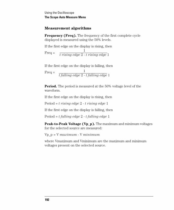
Using the OscilloscopeThe Scope Auto Measure Menu
Measurement algorithms
Frequency (Freq). The frequency of the first complete cycle displayed is measured using the 50% levels.
If the first edge on the display is rising, then
Freq =
If the first edge on the display is falling, then
Freq =
Period. The period is measured at the 50% voltage level of the waveform.
If the first edge on the display is rising, then
Period = t rising edge 2 - t rising edge 1
If the first edge on the display is falling, then
Period = t falling edge 2 - t falling edge 1
Peak-to-Peak Voltage (Vp_p). The maximum and minimum voltages for the selected source are measured:
Vp_p = V maximum - V minimum
where Vmaximum and Vminimum are the maximum and minimum voltages present on the selected source.
1t rising edge 2 - t rising edge 1
1t falling edge 2 - t falling edge 1
192
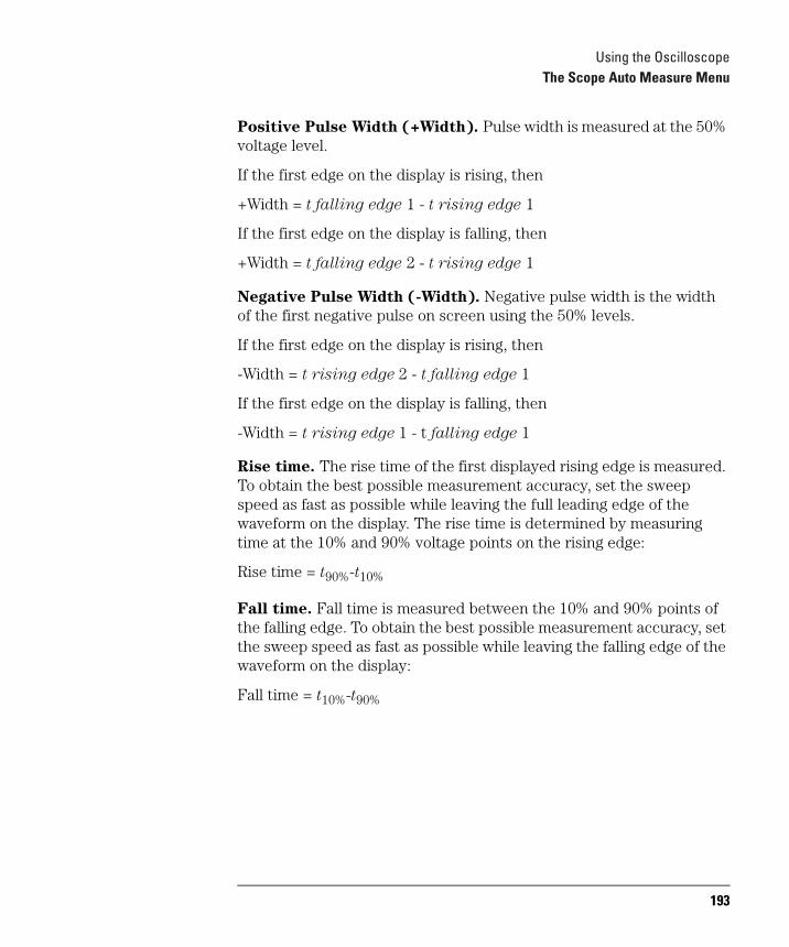
Using the OscilloscopeThe Scope Auto Measure Menu
Positive Pulse Width (+Width). Pulse width is measured at the 50% voltage level.
If the first edge on the display is rising, then
+Width = t falling edge 1 - t rising edge 1
If the first edge on the display is falling, then
+Width = t falling edge 2 - t rising edge 1
Negative Pulse Width (-Width). Negative pulse width is the width of the first negative pulse on screen using the 50% levels.
If the first edge on the display is rising, then
-Width = t rising edge 2 - t falling edge 1
If the first edge on the display is falling, then
-Width = t rising edge 1 - t falling edge 1
Rise time. The rise time of the first displayed rising edge is measured. To obtain the best possible measurement accuracy, set the sweep speed as fast as possible while leaving the full leading edge of the waveform on the display. The rise time is determined by measuring time at the 10% and 90% voltage points on the rising edge:
Rise time = t90%-t10%
Fall time. Fall time is measured between the 10% and 90% points of the falling edge. To obtain the best possible measurement accuracy, set the sweep speed as fast as possible while leaving the falling edge of the waveform on the display:
Fall time = t10%-t90%
193
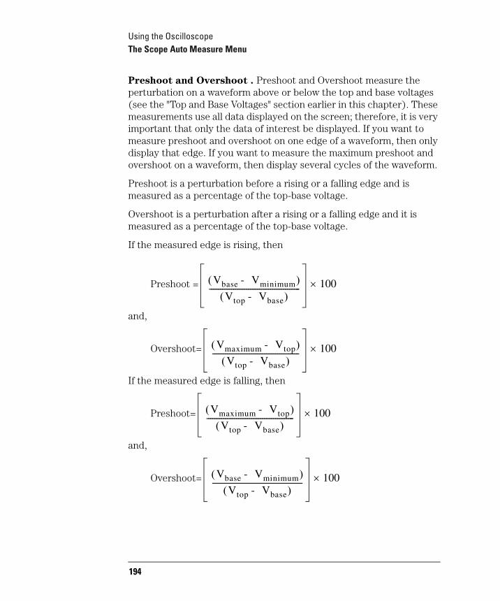
Using the OscilloscopeThe Scope Auto Measure Menu
Preshoot and Overshoot . Preshoot and Overshoot measure the perturbation on a waveform above or below the top and base voltages (see the "Top and Base Voltages" section earlier in this chapter). These measurements use all data displayed on the screen; therefore, it is very important that only the data of interest be displayed. If you want to measure preshoot and overshoot on one edge of a waveform, then only display that edge. If you want to measure the maximum preshoot and overshoot on a waveform, then display several cycles of the waveform.
Preshoot is a perturbation before a rising or a falling edge and is measured as a percentage of the top-base voltage.
Overshoot is a perturbation after a rising or a falling edge and it is measured as a percentage of the top-base voltage.
If the measured edge is rising, then
Preshoot =
and,
Overshoot=
If the measured edge is falling, then
Preshoot=
and,
Overshoot=
Vbase Vminimum-( )Vtop Vbase-( )
------------------------------------------------- 100×
Vmaximum Vtop-( )Vtop Vbase-( )
----------------------------------------------- 100×
Vmaximum Vtop-( )Vtop Vbase-( )
----------------------------------------------- 100×
Vbase Vminimum-( )Vtop Vbase-( )
------------------------------------------------- 100×
194

8
Using the Pattern Generator
195
Using the Pattern GeneratorUsing the Pattern Generator
Using the Pattern GeneratorThis chapter provides instructions for using the pattern generator to generate vectors and patterns for design and test environments. It also covers the pattern generator common menus, loading ASCII files, and the pattern generator probing system.
This chapter covers:
• Setting up the proper configurations
• Building test vectors and functions
• Pattern generator common menus
• Loading ASCII files
• Pattern generator probing system
196
Using the Pattern GeneratorSetting Up the Proper Configurations
Setting Up the Proper ConfigurationsThis section discusses setting up the configuration attributes and parameters of the pattern generator.
If you are reloading existing configurations or downloading ASCII vector files, refer to the Load operation in the disk drive menus of the System.
To set up the configuration
1 From the Format menu, set the Vector Output Mode to either full- or half-channel.
Make this selection first because clock frequencies and available channels are affected.
In half-channel mode, only pods 1 and 3 are used.
2 Set the Clock Source to either internal or external.
An external clock is used when you need a clock frequency that is not available internally, or if you need to drive the pattern generator timing with an external reference.
3 Set the Clock Period for an internal clock or the Clock Frequency for an external clock.
The external clock frequency information is required to select the appropriate operating mode. Operating the pattern generator at an external clock frequency higher than selected will result in erroneous operation.
197
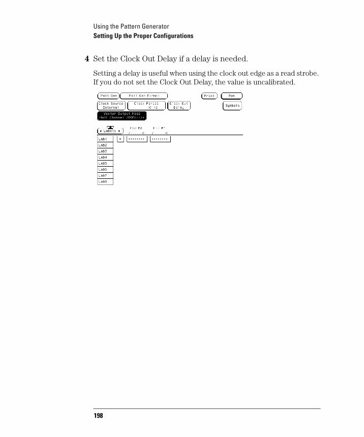
Using the Pattern GeneratorSetting Up the Proper Configurations
4 Set the Clock Out Delay if a delay is needed.
Setting a delay is useful when using the clock out edge as a read strobe. If you do not set the Clock Out Delay, the value is uncalibrated.
198
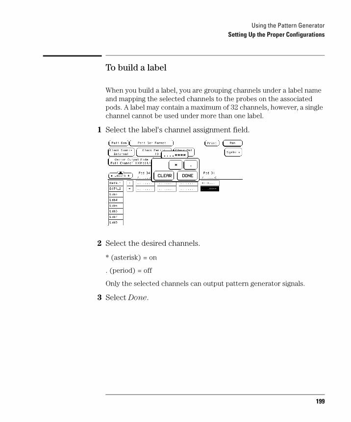
Using the Pattern GeneratorSetting Up the Proper Configurations
To build a label
When you build a label, you are grouping channels under a label name and mapping the selected channels to the probes on the associated pods. A label may contain a maximum of 32 channels, however, a single channel cannot be used under more than one label.
1 Select the label's channel assignment field.
2 Select the desired channels.
* (asterisk) = on
. (period) = off
Only the selected channels can output pattern generator signals.
3 Select Done.
199
Using the Pattern GeneratorBuilding Test Vectors and Functions
Building Test Vectors and FunctionsOnce the pattern generator is configured, you will want to build programs to use in your test system. You build programs in the Sequence menu. If you have small program segments that are built from frequently used vectors, they can be built in the User Macros Sequence menu.
200
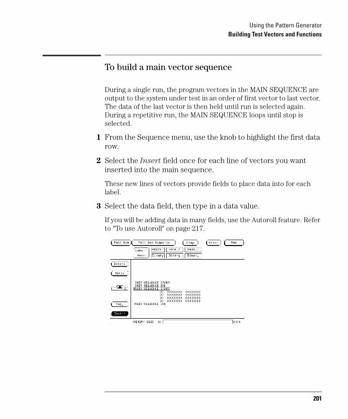
Using the Pattern GeneratorBuilding Test Vectors and Functions
To build a main vector sequence
During a single run, the program vectors in the MAIN SEQUENCE are output to the system under test in an order of first vector to last vector. The data of the last vector is then held until run is selected again. During a repetitive run, the MAIN SEQUENCE loops until stop is selected.
1 From the Sequence menu, use the knob to highlight the first data row.
2 Select the Insert field once for each line of vectors you want inserted into the main sequence.
These new lines of vectors provide fields to place data into for each label.
3 Select the data field, then type in a data value.
If you will be adding data in many fields, use the Autoroll feature. Refer to "To use Autoroll" on page 217.
201
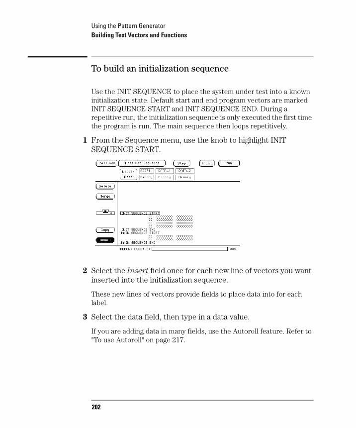
Using the Pattern GeneratorBuilding Test Vectors and Functions
To build an initialization sequence
Use the INIT SEQUENCE to place the system under test into a known initialization state. Default start and end program vectors are marked INIT SEQUENCE START and INIT SEQUENCE END. During a repetitive run, the initialization sequence is only executed the first time the program is run. The main sequence then loops repetitively.
1 From the Sequence menu, use the knob to highlight INIT SEQUENCE START.
2 Select the Insert field once for each new line of vectors you want inserted into the initialization sequence.
These new lines of vectors provide fields to place data into for each label.
3 Select the data field, then type in a data value.
If you are adding data in many fields, use the Autoroll feature. Refer to "To use Autoroll" on page 217.
202
Using the Pattern GeneratorBuilding Test Vectors and Functions
To edit a main or initialization sequence
1 Using the knob, highlight the vector you want to edit.
2 Select the data field you want to edit.
3 Select the new instruction or change the data value.
203
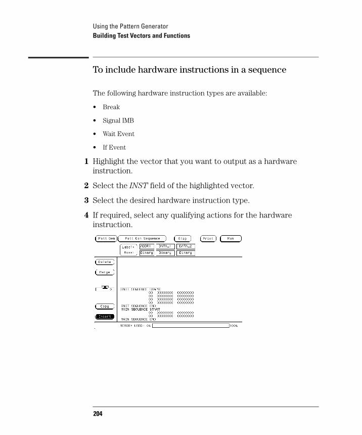
Using the Pattern GeneratorBuilding Test Vectors and Functions
To include hardware instructions in a sequence
The following hardware instruction types are available:
• Break
• Signal IMB
• Wait Event
• If Event
1 Highlight the vector that you want to output as a hardware instruction.
2 Select the INST field of the highlighted vector.
3 Select the desired hardware instruction type.
4 If required, select any qualifying actions for the hardware instruction.
204
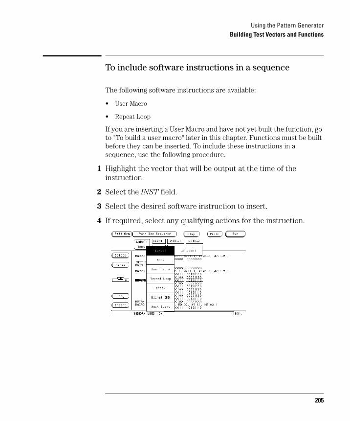
Using the Pattern GeneratorBuilding Test Vectors and Functions
To include software instructions in a sequence
The following software instructions are available:
• User Macro
• Repeat Loop
If you are inserting a User Macro and have not yet built the function, go to "To build a user macro" later in this chapter. Functions must be built before they can be inserted. To include these instructions in a sequence, use the following procedure.
1 Highlight the vector that will be output at the time of the instruction.
2 Select the INST field.
3 Select the desired software instruction to insert.
4 If required, select any qualifying actions for the instruction.
205

Using the Pattern GeneratorBuilding Test Vectors and Functions
To include a user macro in a sequence
If you have user macros, you can include them in the vector sequence using the following procedure. (If you have not yet built user macros, turn to "To build a user macro" to build needed functions.)
1 Insert a new vector where you want to place the user macro.
2 Highlight this new vector using the knob, then select the INST field.
3 Select the User Macro field.
4 Select the user macro you want to insert from the list provided in the pop-up.
206
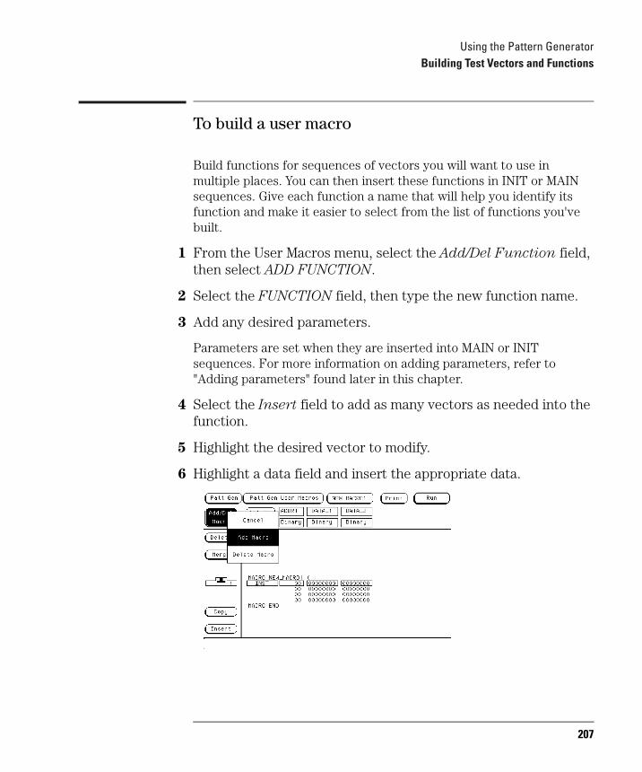
Using the Pattern GeneratorBuilding Test Vectors and Functions
To build a user macro
Build functions for sequences of vectors you will want to use in multiple places. You can then insert these functions in INIT or MAIN sequences. Give each function a name that will help you identify its function and make it easier to select from the list of functions you've built.
1 From the User Macros menu, select the Add/Del Function field, then select ADD FUNCTION.
2 Select the FUNCTION field, then type the new function name.
3 Add any desired parameters.
Parameters are set when they are inserted into MAIN or INIT sequences. For more information on adding parameters, refer to "Adding parameters" found later in this chapter.
4 Select the Insert field to add as many vectors as needed into the function.
5 Highlight the desired vector to modify.
6 Highlight a data field and insert the appropriate data.
207
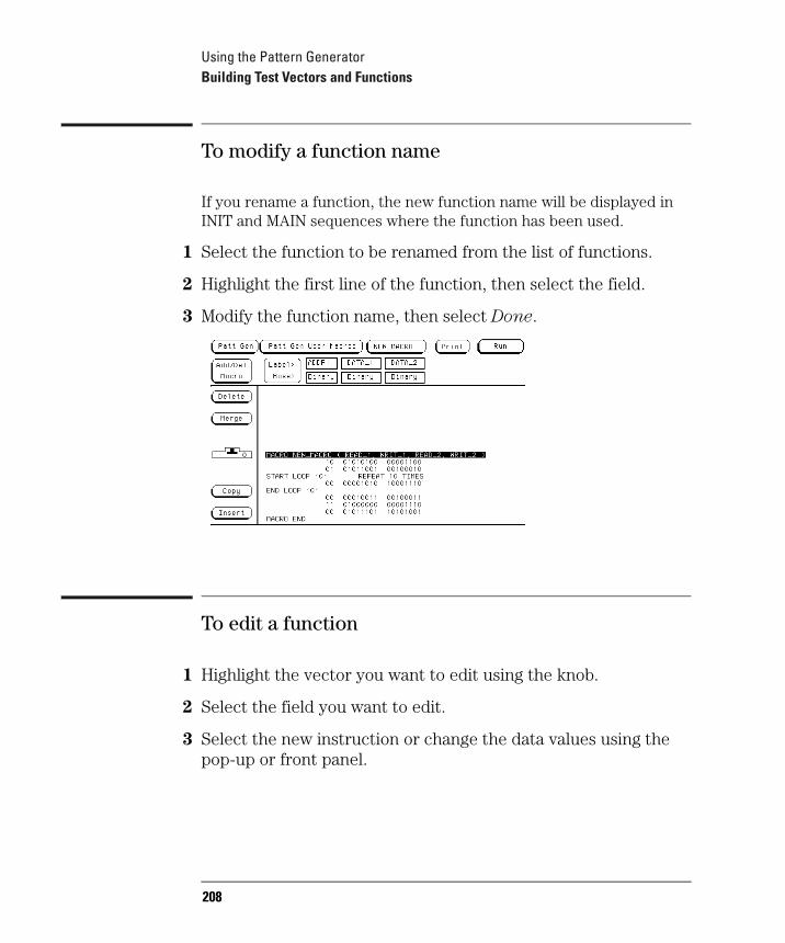
Using the Pattern GeneratorBuilding Test Vectors and Functions
To modify a function name
If you rename a function, the new function name will be displayed in INIT and MAIN sequences where the function has been used.
1 Select the function to be renamed from the list of functions.
2 Highlight the first line of the function, then select the field.
3 Modify the function name, then select Done.
To edit a function
1 Highlight the vector you want to edit using the knob.
2 Select the field you want to edit.
3 Select the new instruction or change the data values using the pop-up or front panel.
208

Using the Pattern GeneratorBuilding Test Vectors and Functions
To add, delete, or rename parameters
Parameters are set when they are inserted into MAIN or INIT sequences. The changes you make in the parameter list will appear every place in the INIT or MAIN sequences in which you have used that function.
1 From the User Macros menu, select a function from the list of functions.
2 Highlight the first line of the function, then select the field.
3 To add a parameter, select Add Parameter, then select the new parameter field that appears and rename the parameter.
4 To delete a parameter from the parameter list, select a parameter name, then select Delete Parameter.
209
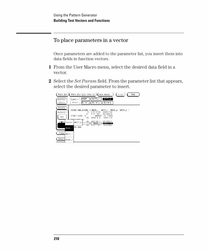
Using the Pattern GeneratorBuilding Test Vectors and Functions
To place parameters in a vector
Once parameters are added to the parameter list, you insert them into data fields in function vectors.
1 From the User Macro menu, select the desired data field in a vector.
2 Select the Set Param field. From the parameter list that appears, select the desired parameter to insert.
210
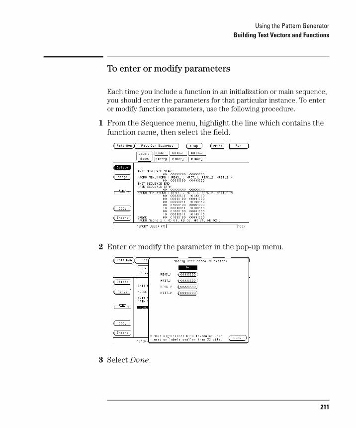
Using the Pattern GeneratorBuilding Test Vectors and Functions
To enter or modify parameters
Each time you include a function in an initialization or main sequence, you should enter the parameters for that particular instance. To enter or modify function parameters, use the following procedure.
1 From the Sequence menu, highlight the line which contains the function name, then select the field.
2 Enter or modify the parameter in the pop-up menu.
3 Select Done.
211
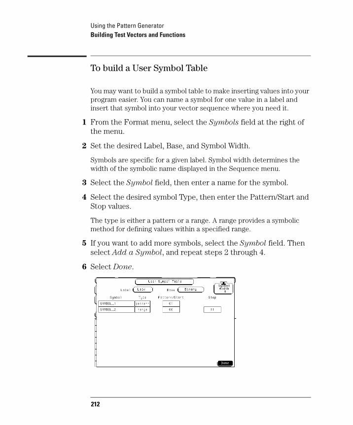
Using the Pattern GeneratorBuilding Test Vectors and Functions
To build a User Symbol Table
You may want to build a symbol table to make inserting values into your program easier. You can name a symbol for one value in a label and insert that symbol into your vector sequence where you need it.
1 From the Format menu, select the Symbols field at the right of the menu.
2 Set the desired Label, Base, and Symbol Width.
Symbols are specific for a given label. Symbol width determines the width of the symbolic name displayed in the Sequence menu.
3 Select the Symbol field, then enter a name for the symbol.
4 Select the desired symbol Type, then enter the Pattern/Start and Stop values.
The type is either a pattern or a range. A range provides a symbolic method for defining values within a specified range.
5 If you want to add more symbols, select the Symbol field. Then select Add a Symbol, and repeat steps 2 through 4.
6 Select Done.
212
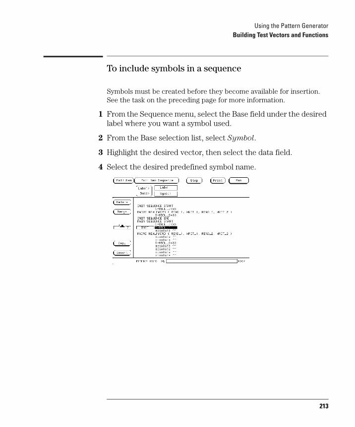
Using the Pattern GeneratorBuilding Test Vectors and Functions
To include symbols in a sequence
Symbols must be created before they become available for insertion. See the task on the preceding page for more information.
1 From the Sequence menu, select the Base field under the desired label where you want a symbol used.
2 From the Base selection list, select Symbol.
3 Highlight the desired vector, then select the data field.
4 Select the desired predefined symbol name.
213
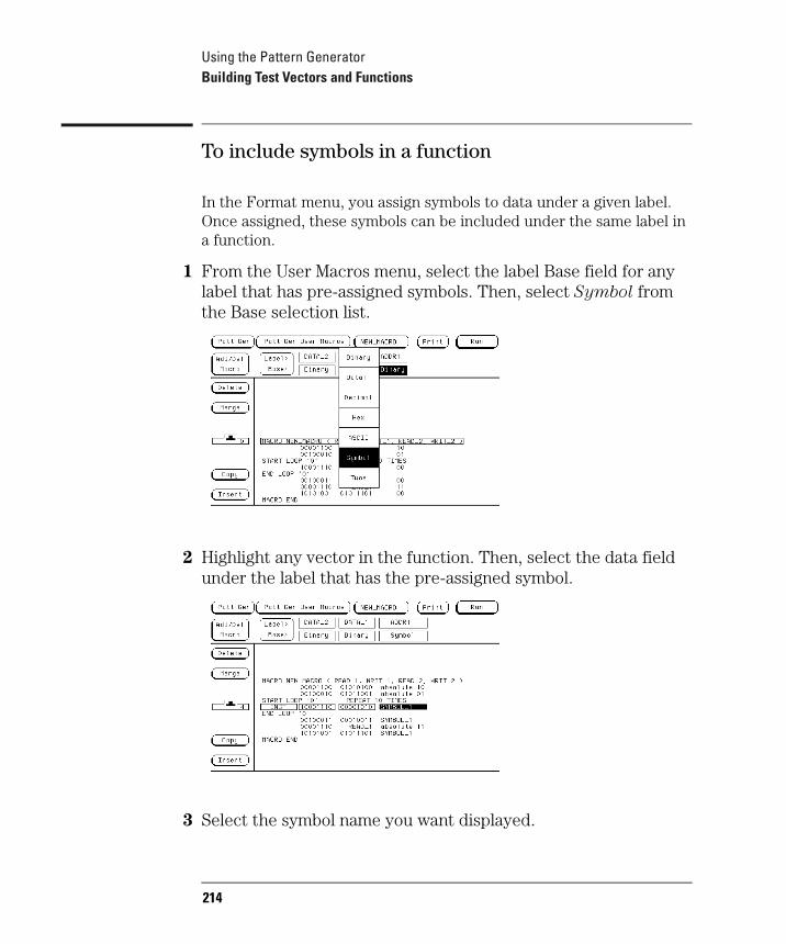
Using the Pattern GeneratorBuilding Test Vectors and Functions
To include symbols in a function
In the Format menu, you assign symbols to data under a given label. Once assigned, these symbols can be included under the same label in a function.
1 From the User Macros menu, select the label Base field for any label that has pre-assigned symbols. Then, select Symbol from the Base selection list.
2 Highlight any vector in the function. Then, select the data field under the label that has the pre-assigned symbol.
3 Select the symbol name you want displayed.
214
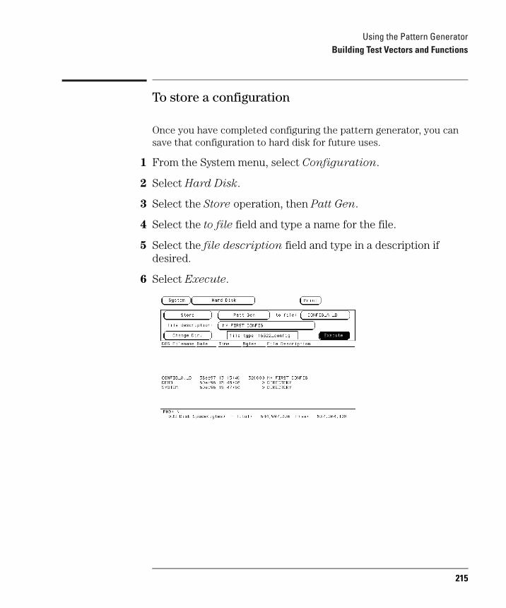
Using the Pattern GeneratorBuilding Test Vectors and Functions
To store a configuration
Once you have completed configuring the pattern generator, you can save that configuration to hard disk for future uses.
1 From the System menu, select Configuration.
2 Select Hard Disk.
3 Select the Store operation, then Patt Gen.
4 Select the to file field and type a name for the file.
5 Select the file description field and type in a description if desired.
6 Select Execute.
215
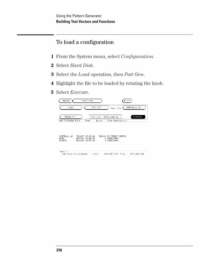
Using the Pattern GeneratorBuilding Test Vectors and Functions
To load a configuration
1 From the System menu, select Configuration.
2 Select Hard Disk.
3 Select the Load operation, then Patt Gen.
4 Highlight the file to be loaded by rotating the knob.
5 Select Execute.
216
Using the Pattern GeneratorBuilding Test Vectors and Functions
To use Autoroll
When Autoroll is used, each time you complete the process of adding data to a data field, the data entry focus changes to the next specified data field. The data entry keypad remains active, ready to define the next data field.
The following procedure shows you how to use Autoroll:
1 Select the first data field to define.
2 Enter the desired data using the pop-up keypad.
3 Select the Autoroll Off field, then select the desired roll direction.
4 As you continue to enter data and select Done, the data field focus rolls to the next data field automatically.
217

Using the Pattern GeneratorBuilding Test Vectors and Functions
The Format Menu
The Format menu lets you configure the pattern generator with a clock source and parameters, generate a symbol table, select its output mode, assign which vector output channels are used, and then group and label the vector output channels.
Format Menu
Clock Source
The Clock Source field toggles between internal and external. The internal clock source is supplied by the pattern generator and controls the frequency the vectors are output to the system under test.
The external clock is provided by you, or the system under test, and is input to the pattern generator through the CLK IN probe of a clock pod. By using an external clock, you synchronize the vector output of the pattern generator to the system under test.
Regardless of which clock is selected, vectors are output on the rising edge of the clock.
218
Using the Pattern GeneratorBuilding Test Vectors and Functions
Clock Period (internal clock source)
This field toggles from Clock Period, when an internal clock source is selected, to Clock Frequency, when an external clock source is selected.
You select clock periods in steps of 1, 2, 2.5, 4, 5, 8, and 10. If the keypad is used to select a value between the step intervals, the value is rounded to the nearest interval.
The minimum clock period available with Vector Output Mode at Full Channel 100 Mbit/s is 10 ns. The minimum clock period available with Vector Output Mode at Half Channel 200 Mbit/s is 5 ns. Maximum clock period for either mode is 250 ms.
Clock Frequency (external clock source)
This field toggles from Clock Frequency, when an external clock source is selected, to Clock Period, when an internal clock source is selected. Set the clock frequency range to match the frequency of the external clock source.
If the Vector Output Mode is Full Channel 100 Mbit/s, you are offered two clock frequency ranges:
• Less than 50 MHz
• Between 50 MHz and 100 MHz
If the Vector Output Mode is Half Channel 200 Mbit/s, you are offered three clock frequency ranges:
• Less than 50 MHz
• Between 50 MHz and 100 MHz
• Greater than 100 MHz
NOTE: If the external clock is faster than the frequency range selected, the pattern generator will produce erroneous output vectors.
219
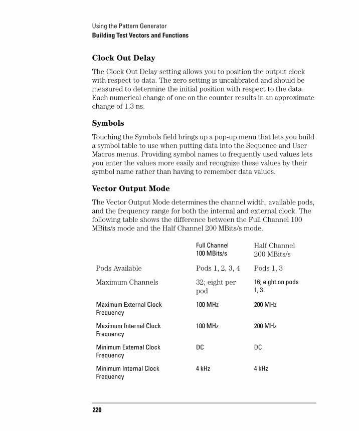
Using the Pattern GeneratorBuilding Test Vectors and Functions
Clock Out Delay
The Clock Out Delay setting allows you to position the output clock with respect to data. The zero setting is uncalibrated and should be measured to determine the initial position with respect to the data. Each numerical change of one on the counter results in an approximate change of 1.3 ns.
Symbols
Touching the Symbols field brings up a pop-up menu that lets you build a symbol table to use when putting data into the Sequence and User Macros menus. Providing symbol names to frequently used values lets you enter the values more easily and recognize these values by their symbol name rather than having to remember data values.
Vector Output Mode
The Vector Output Mode determines the channel width, available pods, and the frequency range for both the internal and external clock. The following table shows the difference between the Full Channel 100 MBits/s mode and the Half Channel 200 MBits/s mode.
Full Channel100 MBits/s
Half Channel 200 MBits/s
Pods Available Pods 1, 2, 3, 4 Pods 1, 3
Maximum Channels 32; eight per pod
16; eight on pods 1, 3
Maximum External Clock Frequency
100 MHz 200 MHz
Maximum Internal Clock Frequency
100 MHz 200 MHz
Minimum External Clock Frequency
DC DC
Minimum Internal Clock Frequency
4 kHz 4 kHz
220

Using the Pattern GeneratorBuilding Test Vectors and Functions
Labels
Labels let the user group output channels from the data pods into a more logical configuration for creating vector data. The pattern generator labels work in the same fashion as the labels for the logic analyzer products, with the exception that an output channel cannot be assigned to more than one label.
221
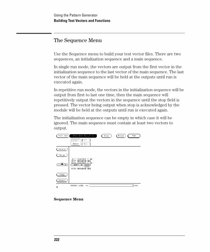
Using the Pattern GeneratorBuilding Test Vectors and Functions
The Sequence Menu
Use the Sequence menu to build your test vector files. There are two sequences, an initialization sequence and a main sequence.
In single run mode, the vectors are output from the first vector in the initialization sequence to the last vector of the main sequence. The last vector of the main sequence will be held at the outputs until run is executed again.
In repetitive run mode, the vectors in the initialization sequence will be output from first to last one time, then the main sequence will repetitively output the vectors in the sequence until the stop field is pressed. The vector being output when stop is acknowledged by the module will be held at the outputs until run is executed again.
The initialization sequence can be empty in which case it will be ignored. The main sequence must contain at least two vectors to output.
Sequence Menu
222
Using the Pattern GeneratorBuilding Test Vectors and Functions
INIT and MAIN Sequences
Use the knob to highlight individual lines in either vector sequences. When a line is highlighted, you can add data lines below it by selecting the Insert field. Selecting the INST field brings up a dialog box that lets you insert one of the instructions or user macros into the vector sequence.
An instruction is not allowed on the following vector lines of the sequence:
• The first vector of the INIT sequence.
• The first vector of the MAIN sequence.
• The last vector of the MAIN sequence.
• The vector prior to the IF block.
• The first vector of the IF block.
• The last vector of the IF block.
• The vector following the IF block.
It should be noted that with the Vector Output Mode of Half Channel 200 Mbit/s, the INIT sequence must contain a number of vectors that is divisible by four. If this is not the case, the first vector of the INIT sequence is duplicated to create the correct number of vectors.
With the Vector Output Mode of Full Channel 100 Mbit/s and vector frequencies greater than 50 MHz, the INIT sequence must contain an even number of vectors. Again, if this is not the case, the first vector of the INIT sequence is duplicated to create the correct number of vectors.
223
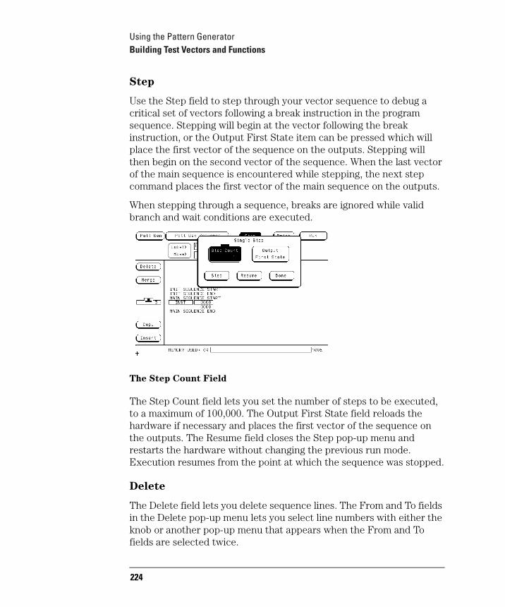
Using the Pattern GeneratorBuilding Test Vectors and Functions
Step
Use the Step field to step through your vector sequence to debug a critical set of vectors following a break instruction in the program sequence. Stepping will begin at the vector following the break instruction, or the Output First State item can be pressed which will place the first vector of the sequence on the outputs. Stepping will then begin on the second vector of the sequence. When the last vector of the main sequence is encountered while stepping, the next step command places the first vector of the main sequence on the outputs.
When stepping through a sequence, breaks are ignored while valid branch and wait conditions are executed.
The Step Count Field
The Step Count field lets you set the number of steps to be executed, to a maximum of 100,000. The Output First State field reloads the hardware if necessary and places the first vector of the sequence on the outputs. The Resume field closes the Step pop-up menu and restarts the hardware without changing the previous run mode. Execution resumes from the point at which the sequence was stopped.
Delete
The Delete field lets you delete sequence lines. The From and To fields in the Delete pop-up menu lets you select line numbers with either the knob or another pop-up menu that appears when the From and To fields are selected twice.
224

Using the Pattern GeneratorBuilding Test Vectors and Functions
When deleting vector rows, the INIT START, INIT END, MAIN START, and MAIN END cannot be deleted. Deleting all the vector rows from INIT START to MAIN END will reset the sequence to the powerup state. The deletion will not be performed if the results of the delete operation will place fewer than two vectors in the main sequence, or, if the delete operation will place an instruction on any of the following vectors:
• The first vector of the INIT sequence.
• The first vector of the MAIN sequence.
• The last vector of the MAIN sequence.
• The vector prior to the IF block.
• The first vector of the IF block.
• The last vector of the IF block.
• The vector following the IF block.
Merge
Selecting the Merge field brings up a pop-up menu that lets you select sections of a previously created configuration file to merge after the current line in the sequence. The Input Drive field selects between the hard disk or the front floppy disk (if present). The Filename field displays a file browser pop-up menu that allows searching for the file to be used in the merge. The Merge Section field lets you select the section of the configuration to be merged. Configuration sections consist of the main sequence and any functions that were created. The merge will not be performed in the following cases:
• Merge data exceeds the maximum number of sequence lines.
• Merge data requires more repeats than are available.
• Merge data requires more function calls than are available.
225
Using the Pattern GeneratorBuilding Test Vectors and Functions
Merge is not allowed in the following cases:
• Within a repeat loop.
• Within an IF block (starting with the vector prior to the if, and ending with the vector following the IF).
• Between the start and first vector of the main sequence.
• After the last vector of the main sequence.
• Between the init and main sequence.
• Between the start and first vector of the init sequence.
• Within an empty init sequence (insert one vector in the init and merge after that vector).
Copy
Selecting the Copy field brings up a pop-up menu that lets you select vector sequence lines to be copied and a location to insert them. The values in the Start, End, and Copy After fields can be selected with the knob or with the pop-up keypad that appears when the appropriate field is selected twice.
Copy will not be performed if you run out of function calls (1000) or repeats (1000). Copy will not be allowed if the result of the copy places an instruction on one of the following vectors:
• The first vector of the INIT sequence.
• The first vector of the MAIN sequence.
• The last vector of the MAIN sequence.
• The vector prior to the IF block.
• The first vector of the IF block.
• The last vector of the IF block.
• The vector following the IF block.
226
Using the Pattern GeneratorBuilding Test Vectors and Functions
Insert
Selecting the Insert field adds another instruction line immediately below the line that is currently highlighted.
Instructions
User Macro. The User Macro instruction brings up a list of current user macros you can insert. Functions are inserted at the current line and expanded at run time.
If the function selected has parameters, a second pop-up menu will be displayed to allow setting of the passed parameter values. Parameters are passed as 32 bit values and the most significant bits are truncated when the data is applied to labels with less than 32 bits.
Once inserted, the passed parameters of a function may be altered by selecting that function again and changing the data. A function can only be removed from the sequence by using the delete field.
Repeat Loop. The Repeat Loop instruction inserts the start and end of a repeat loop using the current vector row as the data. Once the loop has been created, vectors can be inserted or copied into the loop to change the size. A repeat loop will be expanded at run time into individual vectors. The number of repetitions of the loop (maximum 20000) is set when the repeat is first inserted into the sequence and can be altered by selecting the start of the repeat to get the Repeat Count pop-up menu. Both the start and end of a repeat loop will be removed from the sequence if either is included in the delete block.
227
Using the Pattern GeneratorBuilding Test Vectors and Functions
Break. The Break instruction causes a break at the current vector. In single run mode, this instruction halts the sequence and holds the outputs at the break vector's value. In repetitive run mode, this instruction pauses the sequence at the current vector momentarily, then continues.
NOTE: When operating at 200 MHz you can not have 2 Break events in succession. This also includes the Wait event.
Signal IMB. The Signal IMB instruction creates a signal for the IMB bus of the 1670G-series at the current vector, allowing the pattern generator to trigger the state or timing analyzers. Multiple signal IMB instructions may be placed in the sequence, but only the first signal IMB will be executed.
Wait Event. The Wait Event instruction halts the execution of the program sequence until the event is received by the hardware. Selecting this instruction brings up a pop-up menu that lets you set four data patterns and select one of them or an IMB signal as the event the pattern generator is waiting for.
An external wait event is the ORing of the three input lines on the clock pod. The first wait IMB is the only one recognized because IMB does not allow pulsing.
NOTE: When operating at 200 MHz you can not have 2 Wait events in succession. This also includes the Break event.
If Event. The If Event instruction is only available in Full Channel 100 Mbit/s mode with clock frequencies of 50 MHz and lower. Only one If Event is allowed in a sequence program. If a new if instruction is placed in a program sequence, a message will appear stating that only one if instruction is allowed. To add a new if instruction, the old one must be deleted.
228
Using the Pattern GeneratorBuilding Test Vectors and Functions
The If event uses either the IMB or the same external clock pod input lines as the Wait event. If the condition is true at the If event, then the data in the If block is output, otherwise it is skipped.
The If event takes the current data line and duplicates as in the following example:
These vectors are now restricted. They cannot have instructions. Delete and Copy operations that result in instructions being placed on these vectors will not be allowed. The If can be removed by deleting either the start or end of the If block.
current dataIF
current datacurrent data
END IFcurrent data
These vectors are now restricted. They cannot have instructions. Delete and Copy operations that result in instructions being placed on these vectors will not be allowed. The If can be removed by deleting either the start or end of the If block.
229
Using the Pattern GeneratorBuilding Test Vectors and Functions
Data Field
Selecting the data field to the right of the instruction field lets you insert vector data. ASCII-based data cannot be edited, and ASCII- and Symbols-based data cannot be autorolled.
Autoroll
The Autoroll field is provided to reduce the number of keystrokes required to enter data into the sequence or a function. When a data field is edited (except in the last vector row), the Autoroll field appears to the left of the data entry pop-up menu. Autoroll can move from left to right across the labels on the display with an automatic line feed, or it can move down a label from vector row to row. When the last vector row of the sequence is encountered, Autoroll will stop the editing process, or the Autoroll can be halted at any point in the editing process by turning the autoroll function off.
Memory Used
The MEMORY USED bar shows in percent how much memory is being used by the vector sequence entered. It should be noted that Repeat Loops and User Macros may suddenly increase the amount of memory used because they are expanded at run time. It is critical to use the MEMORY USED bar to obtain an idea of how much memory will be needed at run time.
230
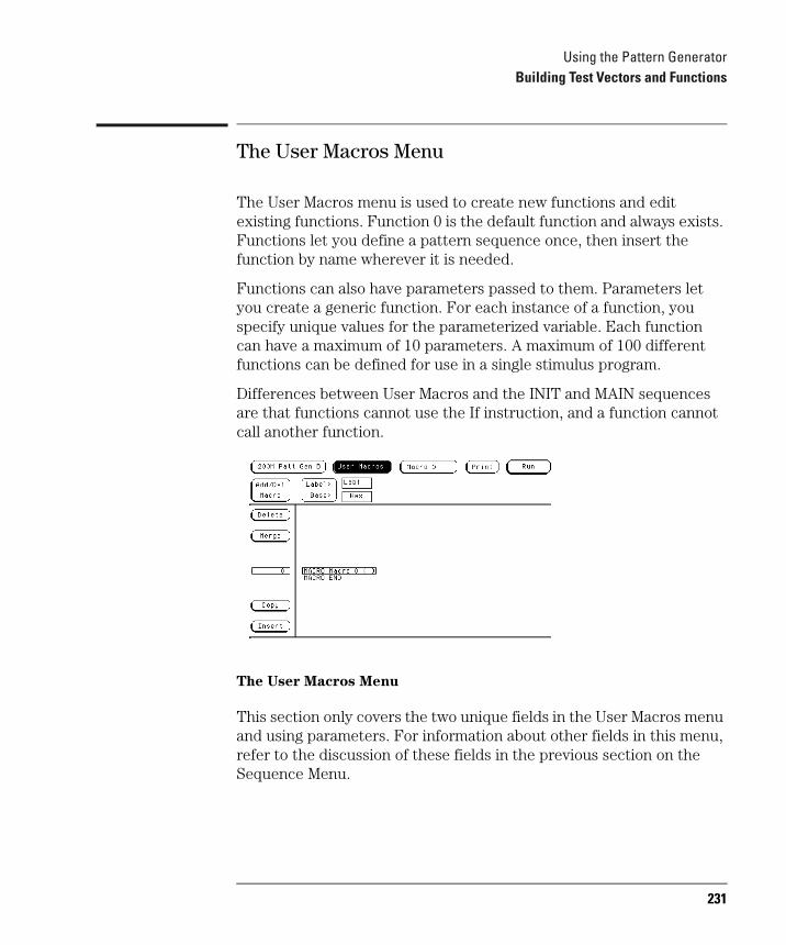
Using the Pattern GeneratorBuilding Test Vectors and Functions
The User Macros Menu
The User Macros menu is used to create new functions and edit existing functions. Function 0 is the default function and always exists. Functions let you define a pattern sequence once, then insert the function by name wherever it is needed.
Functions can also have parameters passed to them. Parameters let you create a generic function. For each instance of a function, you specify unique values for the parameterized variable. Each function can have a maximum of 10 parameters. A maximum of 100 different functions can be defined for use in a single stimulus program.
Differences between User Macros and the INIT and MAIN sequences are that functions cannot use the If instruction, and a function cannot call another function.
The User Macros Menu
This section only covers the two unique fields in the User Macros menu and using parameters. For information about other fields in this menu, refer to the discussion of these fields in the previous section on the Sequence Menu.
231

Using the Pattern GeneratorBuilding Test Vectors and Functions
Function 0 (current function field)
Touching this field brings up a list of functions that have been created and are available to insert into the Sequence menu. If you want to edit or view a previously built function, select that function from the list and it will appear in the main part of the display.
Add/Delete Function
Selecting this field brings up a pop-up menu that lets you choose between adding a new function or deleting one. If you select Add Function, a new blank function appears in the display with a new Function "n" name.
To rename the new function, select the function name field, and in the pop-up menu that appears, type in a new name. You can also add parameters to the new function in the same pop-up menu. For more information on parameters, refer to "Using Parameters" below.
If you select Delete Function, you will be presented with a list of current functions. Select the function you want to delete from the list. If the function you delete is being used in the MAIN sequence, it will be removed from the sequence. If you try to delete the first function, it will be removed from the MAIN sequence but not from the function list.
Using Parameters
Parameters are used to pass values into functions. A major benefit in passing parameters is that you keep a function's functionality generic and still direct specific action identified by parameters. Think of parameters as the only part of a function that changes as the function is reused. You create the function and add parameters to the function in the User Macro menu. You then insert the function and assign parameter values in the Sequence menu. As you reuse the function in other places in the sequence, simply change parameter values to the new specific values.
Function parameters are passed as 32-bit values. If fewer than 32 bits are assigned to a label in the Format menu, the most significant bits of the parameter value are truncated when the parameter is used as data for the given label.
232
Using the Pattern GeneratorLoading ASCII Files
Loading ASCII FilesYou can create pattern generator files and load them as ASCII files using one of the remote communication interfaces or by loading an ASCII disk file.
Regardless of the load method selected, the general format of the file must conform to certain guidelines. In general, an ASCII file consists of a block of setup information (clock specs, labels, etc.) followed by a block of pattern generator data.
There are a few minor differences between the format required for a communication download and that of a disk file load.
Disk files are loaded into the pattern generator using the LOAD command on the disk menu.
Some general restrictions are:
• Data is assumed to be entirely hexadecimal base.
• No instructions are allowed in the data.
• No functions are defined or invoked in the data.
• All labels consist of adjacent bits.
A special "ASCII 000000" string is required to uniquely identify an ASCII disk file. This string cannot be used when loading ASCII files using one of the remote communication interfaces. This line must be the first line of the disk file. It consists of 5 blanks and 6 zeros.
233
Using the Pattern GeneratorASCII File Commands
ASCII File CommandsIn addition to the unique ASCII file commands described here, you may want to include some standard FORMat commands in the ASCII file, such as those that are used to specify the clock or output mode.
The only FORMat commands that are permitted are FORMat: MODe, CLOCk, and DELay. Refer to the command descriptions in this chapter for the syntax of these commands.
Note that there is no section header prefix for these ASCII file command strings.
Refer to the example programs at the end of this chapter for usage examples of the various commands described in this chapter.
ASCDown Command
Command ASCDown
The ASCDown command is used to signal the start of an ASCII file load. It causes the current pattern generator label and sequence structures to be cleared and reset to a default state.
The ASCDown command must precede any label definitions and the data portion of an ASCII file load.
Example ASCDown
234
Using the Pattern GeneratorASCII File Commands
LABel
Command LABel <name_str>,<width>
<name_str> label string, six characters maximum in length.
<width> integer number of bits in the label (1 through 32).
The LABel command is a special means of specifying labels for use by an ASCII file. The label bits are assigned from most to least significant bits across the output pods. Labels may only contain adjacent bits. The user must specify the label string and the width of the field. The label base is hexadecimal.
There is a maximum of 126 labels. No label may be more than 32 bits wide. If a label is too wide (too many bits) for the remaining unused pattern generator bits, it will be discarded. Use of the FORMat:LABel command after the ASCDown command will generate an error.
Example LABel 'TEST1',7
LABel 'ADDR',13
235
Using the Pattern GeneratorASCII File Commands
VECTor
Command VECTor <char_count>
<char_count> a ten character string starting with a '#8' and including the total file size count.
The VECTor command is used after the end of the header/setup commands to signal the start of the actual pattern generator data in an ASCII file.
The VECTor command is used with a parameter that specifies the exact byte count of the data block. This count must include all data characters, all blank characters, and all line termination (DOS cr/lf or UNIX cr) characters. The file character count is the sole criteria used to determine when the bus file transfer is complete. If a disk file is used, the character count has no meaning and can be any value or deleted from the command string.
If the file character count does not match the actual data byte count of the file, an error condition will occur. If the actual data count exceeds the byte count passed in with the VECTor command, excess data will be lost (and treated as remote control bus command(s)). If the actual data count is less than the data count passed in with the VECTor command, the bus transfer will appear to hang while the 1670G-series system waits for the 'remaining' data. The controller sending the file may, or may not, time-out and terminate the bus transfer. Generally, recovery from this condition involves sending more data until the data byte count is satisfied.
The file character count is contained in a string with a specific format. The actual count is right justified in a ten-character string that starts with a '#8' followed by eight digits. These ten characters are NOT part of the file character count.
The following page shows an example of this.
236
Using the Pattern GeneratorASCII File Commands
No data is allowed in the same line as the VECTor command. The line termination in the VECTor command line is included in the character count for the file.
The <char_count> field is not required as part of the VECTor command when creating a disk file, and will be ignored if included.
Example VECTor #800010457
Vector Data
The data portion of the ASCII file is basically an array of hexadecimal data fields. Each row of the array corresponds to a single line of the main program. Each column of the array corresponds to a single label as defined on the format menu.
Data fields are separated by one or more blank characters. A line termination (carriage return or carriage return + line feed) signals the end of a line and the start of a new line. If a data field has more data than the label width would indicate, only the least significant bits of the data field are used. If there are more data fields in a row than there are labels, the extra data fields (last data fields in the row) are ignored. If there are fewer data fields in a row than there are labels, the data for the extra (right-most) labels will be zero.
Data lines consisting of only line termination characters are ignored.
The MAIN SEQUENCE must have at least two data lines. In the ASCII data file, a row consisting of only '*M' is used to signal the start of the main sequence. If there is to be no data in the init sequence, the first row of the file after the VECTor command must be '*M'. Note that the quotes in '*M' are not really in the file. The line termination after the '*M' (as well as the '*M') must be included in the character count for a file loaded using a remote bus.
237
Using the Pattern GeneratorASCII File Commands
Any characters that are not valid hexadecimal digits (0 through 9, or upper/lower case a through f) are ignored and treated as field separators. This could cause problems if a typo appears in the middle of a data value (for example, '12R4' will be assigned to two labels as '12' and '4').
The last data row of the file must end with a line termination as this is the flag to load the data row into the data structure. Failure to do this will result in a short main program.
When counting file characters be aware of how a particular file generator (editor) terminates a line. DOS-based systems use two characters. Be sure to account for line termination character(s) in the overall file character count.
The ASCII file load mechanism assumes correctness in the data file and any header commands. Error handling is rather basic, and treating unexpected characters as field separators could create bizarre results when parsing the file. Error messages point to the line number where the parser thinks the error occurred, but the line count may not be exact because of parsing problems with the data.
When using a LAN interface to send ASCII data, an extra line feed <lf> is required at the end of the file. This <lf> is NOT included in the <char_count> value. It is required to ensure the data buffer is flushed.
Serious problems will cause the default main program to be loaded in an effort to avoid locking up the 1670G-series system.
238

Using the Pattern GeneratorASCII File Commands
FORMat:xxx
Command FORMat:MODEFORMat:CLOCkFORMat:DELay
These commands transfer set fields from the Format menu. The existing clock scheme is used if nothing is specified here. Command syntax is same as normal bus commands.
Examples FORMat:MODE FULLFORMat:CLOCk INT,5E-9FORMat:DELay 1E-9
239

Using the Pattern GeneratorASCII File Commands
Loading an ASCII file over a bus (example)
To load an ASCII file over the bus use the following example. A few items to be noted:
• Line numbers are added for documentation only and are NOT part of the actual remote bus commands.
• In this example, the string '<lf>' is a generic line feed sequence and counts as a single character.
010 SELect <slot><lf>
020 ASCDOWN<lf>
030 FORM:MODE FULL<lf>
040 LABEL 'LAB1',8<lf>041 LABEL 'DATA',8<lf>042 LABEL 'TEST',9<lf>043 LABEL 'CLK',3<lf>044 LABEL 'BIG',12<lf>
050 VECT #800000092<lf>060 12 34 56 7 89A<lf>070 0 22 7 0 FFF<lf>080 A0 33 00 1 111<lf>090 *M<lf>100 92 6F 00 1 FF0<lf>110 CA CA 00 1 00F<lf>120 00 10 11 0 ABC<lf>
240
Using the Pattern GeneratorASCII File Commands
Notes
• Lines 010 through 044 can be sent as discrete remote control commands or included in a single file (with the data) and loaded using the bus.
• Other format commands could be used in place of or in addition to line 030.
• The label sequence seen in lines 040 through 044 will result in a specific bit assignment. A different ordering of the LABel commands would give a different ordering to the bits.
• There is a space before the '#8' in line 050.
• The character count in line 050 is based on:
• 15 characters (10 digits, 4 blanks, 1 <lf>) each in lines 060, 080, 100, 110, and 120
• 3 characters in line 090
• 13 characters in line 070
• 1 character (the <lf>) in line 050
Format Specification
Clock Source: Internal
Vector Output Mode: Full Channel 100 Mbit/s
Clock Period: 10 ns
Clock Out Delay Setting: 0
241
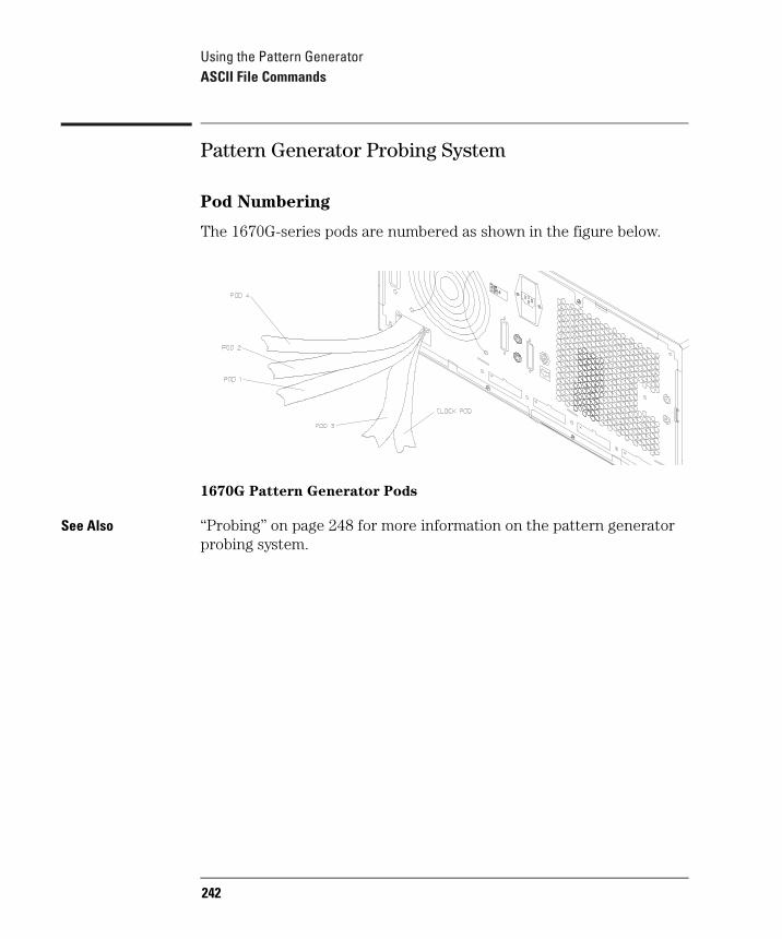
Using the Pattern GeneratorASCII File Commands
Pattern Generator Probing System
Pod Numbering
The 1670G-series pods are numbered as shown in the figure below.
1670G Pattern Generator Pods
See Also “Probing” on page 248 for more information on the pattern generator probing system.
242

9
Logic Analyzer Reference
243

Logic Analyzer Reference1670G-Series Logic Analyzer Description
1670G-Series Logic Analyzer DescriptionThe 1670G-series logic analyzers are part of a family of general-purpose logic analyzers. The 1670G-series consists of four models ranging in channel width from 34 channels to 136 channels, with 150-MHz state and 500-MHz timing speeds. There are two options that expand the use of the 1670G-series. The oscilloscope option, which is a 2-GSa/s digitizing oscilloscope, and the pattern generator option, which is a 200 M Vector/s pattern generator.
The 1670G-series logic analyzers are all designed as full-featured standalone or network-configurable instruments for use by digital and microprocessor hardware and software designers. All models have GPIB, RS-232-C, and Centronics interfaces for hard copy printouts and control by a host computer, and have ethernet LAN interfaces.
Analyzer memory depth is 64K per channel in all pod pair groupings, or 128K per channel on one pod of a pod pair (half-channel mode). Deeper memory configurations are available as options (see page 92).
Measurement data is displayed as data listings and waveforms, and can also be plotted on a chart or compared to a reference image. Profiled data is displayed as histograms of activity by time, state, or address range using the software performance analysis feature.
The 150-MHz state analyzer has master, master/slave, and demultiplexed clocking modes available. Measurement data can be stamped with state or time tags. For triggering and data storage, the state analyzer uses 12 sequence levels with two-way branching, 10 pattern resource terms, 2 range terms, and 2 timers.
The 250-MHz timing analyzer has conventional timing mode with variable width, depth, and speed selections. Sequential triggering uses 10 sequence levels with two-way branching, 10 pattern resource terms, 2 range terms, 2 edge terms and 2 timers.
244
Logic Analyzer Reference1670G-Series Logic Analyzer Description
Oscilloscope option
The 2 GSa/s oscilloscope has immediate, edge, and pattern trigger modes. The pattern trigger mode uses both channels, an occurrence counter, and a timer for specifying complex patterns. The oscilloscope also provides statistics and nine automatic measurements. Oscilloscope memory is 32K samples.
Pattern generator option
The 200 M Vector/s pattern generator has a memory depth of 258,048 vectors with a maximum of 32 channels of digital stimulus.
245

Logic Analyzer Reference1670G-Series Configuration Capabilities
1670G-Series Configuration CapabilitiesThe four analyzer models in each of the 1670GP-series offer a wide variety of channel widths and memory depth combinations. The number of data channels range from 34 channels with the 1673G, to a maximum of 136 channels with the 1670G. In addition, a half-channel acquisition mode is available which doubles memory depth per channel while reducing channel width by half.
The configuration guide below illustrates the memory depth/channel width combinations in all acquisition modes with all analyzer models.
State Analyzer Configurations
State Analyzer Configuration Considerations
• Unused clock channels can be used as data channels.
• With Time or State tags turned on, memory depth is reduced by half. However, full depth is retained if you leave one pod pair unassigned.
• Deeper memory configurations are available as options (see page 92).
Mode Memory 1670G 1671G 1672G 1673G
Full-channel 150 MHz
65536 (64K)
64K-deep / 136 chan. 132 data + 4 data or clock
64K-deep / 102 chan. 98 data + 4 data or clock
64K-deep / 68 chan. 64 data +4 data or clock
64K-deep / 34 chan. 32 data + 2 data or clock
246
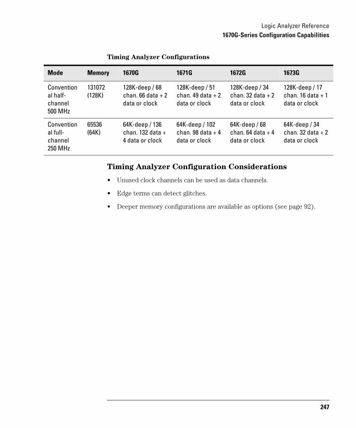
Logic Analyzer Reference1670G-Series Configuration Capabilities
Timing Analyzer Configurations
Timing Analyzer Configuration Considerations
• Unused clock channels can be used as data channels.
• Edge terms can detect glitches.
• Deeper memory configurations are available as options (see page 92).
Mode Memory 1670G 1671G 1672G 1673G
Conventional half-channel500 MHz
131072 (128K)
128K-deep / 68 chan. 66 data + 2 data or clock
128K-deep / 51 chan. 49 data + 2 data or clock
128K-deep / 34 chan. 32 data + 2 data or clock
128K-deep / 17 chan. 16 data + 1 data or clock
Conventional full-channel 250 MHz
65536 (64K)
64K-deep / 136 chan. 132 data + 4 data or clock
64K-deep / 102 chan. 98 data + 4 data or clock
64K-deep / 68 chan. 64 data + 4 data or clock
64K-deep / 34 chan. 32 data + 2 data or clock
247
Logic Analyzer ReferenceProbing
ProbingThis section discusses the probing system for the logic analyzer. It also contains the information you need for connecting the probe system components to each other, to the logic analyzer, to the oscilloscope, to the pattern generator, and to the system under test.
Probing Options
You can connect the logic analyzer to your system under test in one of the following ways:
• Microprocessor- and bus-specific interfaces (optional).
• Standard general-purpose probing (provided).
• Direct connection to a 20-pin, 3M-Series type header connector using the optional termination adapter.
See Also Accessories for Agilent Logic Analyzers for additional information about the microprocessor interface kits and for any new probing solutions.
248

Logic Analyzer ReferenceProbing
Microprocessor and Bus-Specific Interfaces
There are a number of microprocessor- and bus-specific interfaces available as optional accessories. Microprocessors are supported by Universal Interfaces or Analysis Probes, or in some cases, both.
Universal Interfaces are manufactured by other vendors. Universal Interfaces are aimed at initial hardware turn-on, and provide fast, reliable, and convenient connections to the microprocessor system. Many use passive probing and do not support inverse assembly.
Analysis probes are aimed at hardware turn-on and hardware/software integration, and provide the following:
• All clocking and demultiplexing circuits needed to capture the system's operation.
• Additional status lines to further decode the operation of the CPU.
• Inverse assembly software to translate logic levels captured by the logic analyzer into microprocessor mnemonics.
Bus interfaces will support bus analysis for the following:
• Bus support for GPIB, RS-232-C, RS-449, SCSI, VME, and VXI.
General-Purpose Probing
General-purpose probing connects the logic analyzer probes directly to your target system without using any interface. General-purpose probing does not limit you to specific hookup schemes.
General-purpose probing uses grabbers that connect to both through-hole and surface-mount components. General-purpose probing comes as the standard probing option. You will find a full description of its components and use later in this section.
249

Logic Analyzer ReferenceProbing
The Termination Adapter
The logic analyzer must be properly terminated to operate correctly. Most Agilent Technologies analysis probes have properly terminated state connectors; however, many of them require termination adapters for the timing connectors.
The optional termination adapter lets you connect the logic analyzer probe cables directly to test ports on your target system without the probes.
The termination adapter is designed to connect to a 20-position (2x10), 4-wall, low-profile, header connector which is a 3M-Series 3592 or equivalent.
Termination Adapter
250

Logic Analyzer ReferenceProbing
General-purpose probing system description
The standard probing system provided with the logic analyzer consists of a probe tip assembly, probe cable, and grabbers. Because of the passive design of the probes, there are no active circuits at the outer end of the cable. The rest of this chapter is dedicated to general-purpose probing.
The passive probing system is similar to the probing system used with high-frequency oscilloscopes. It consists of a series RC network (100k ohms in parallel with 1.5 pF) at the probe tip, and a shielded, resistive transmission line. The advantages of this system include the following:
• 1.5-pF input capacitance at the probe tip for minimal loading
• Signal ground at the probe tip for high-speed timing signals
• Inexpensive, removable probe tip assemblies
Probe Tip Assemblies
Probe tip assemblies lets you connect the logic analyzer directly to the target system. This general-purpose probing is useful for discrete digital circuits. Each probe tip assembly contains 16 probe leads (data channels), 1 clock lead, a pod ground lead, and a ground tap for each of the 16 probe leads.
Probe Tip Assembly
251
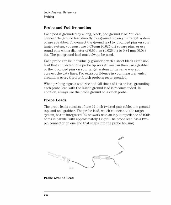
Logic Analyzer ReferenceProbing
Probe and Pod Grounding
Each pod is grounded by a long, black, pod ground lead. You can connect the ground lead directly to a ground pin on your target system or use a grabber. To connect the ground lead to grounded pins on your target system, you must use 0.63-mm (0.025-in) square pins, or use round pins with a diameter of 0.66 mm (0.026 in) to 0.84 mm (0.033 in). The pod ground lead must always be used.
Each probe can be individually grounded with a short black extension lead that connects to the probe tip socket. You can then use a grabber or the grounded pins on your target system in the same way you connect the data lines. For extra confidence in your measurements, grounding every third or fourth probe is recommended.
When probing signals with rise and fall times of 1 ns or less, grounding each probe lead with the 2-inch ground lead is recommended. In addition, always use the probe ground on a clock probe.
Probe Leads
The probe leads consists of one 12-inch twisted-pair cable, one ground tap, and one grabber. The probe lead, which connects to the target system, has an integrated RC network with an input impedance of 100k ohms in parallel with approximately 1.5-pF. The probe lead has a two-pin connector on one end that snaps into the probe housing.
Probe Ground Lead
252
Logic Analyzer ReferenceProbing
Grabbers
The grabbers have a small hook that fits around the IC pins and component leads. The grabbers have been designed to fit on adjacent IC pins on either through-hole or surface-mount components with lead spacing greater than or equal to 0.050 inches.
Probe Cable
The probe cable contains 18 signal lines, 17 chassis ground lines and two power lines for analysis probe use. The cables are woven together into a flat ribbon that is 4.5 feet long. The probe cable connects the logic analyzer to the pods, termination adapter, or analysis probe. Each cable is capable of carrying 0.33 amps for analysis probe power.
CAUTION: DO NOT exceed 0.33 amps per cable, or the cable will be damaged.
Analysis probe power is protected by a current limiting circuit. If the current limiting circuit is activated, the fault condition must be removed. After the fault condition is removed, the circuit will reset in one minute.
Minimum Signal Amplitude
Any signal line you intend to probe with the logic analyzer probes must supply a minimum voltage swing of 500 mV to the probe tip. If you measure signal lines with a voltage swing of less than 500 mV, you may not obtain a reliable measurement. Because the minimum input overdrive is the greater of 250 mV or 30% of input amplitude, be sure to correctly set the pod threshold in the Analyzer Format menu.
253
Logic Analyzer ReferenceProbing
Maximum Probe Input Voltage
The maximum input voltage of each logic analyzer probe is 40 volts peak.
Pod Thresholds
Logic analyzer pods have two preset thresholds and a user-definable pod threshold. The two preset thresholds are ECL (-1.3 V) and TTL (+1.5 V). The user-definable threshold can be set anywhere between -6.0 volts and +6.0 volts in 0.05 volt increments.
All pod thresholds are set independently.
254
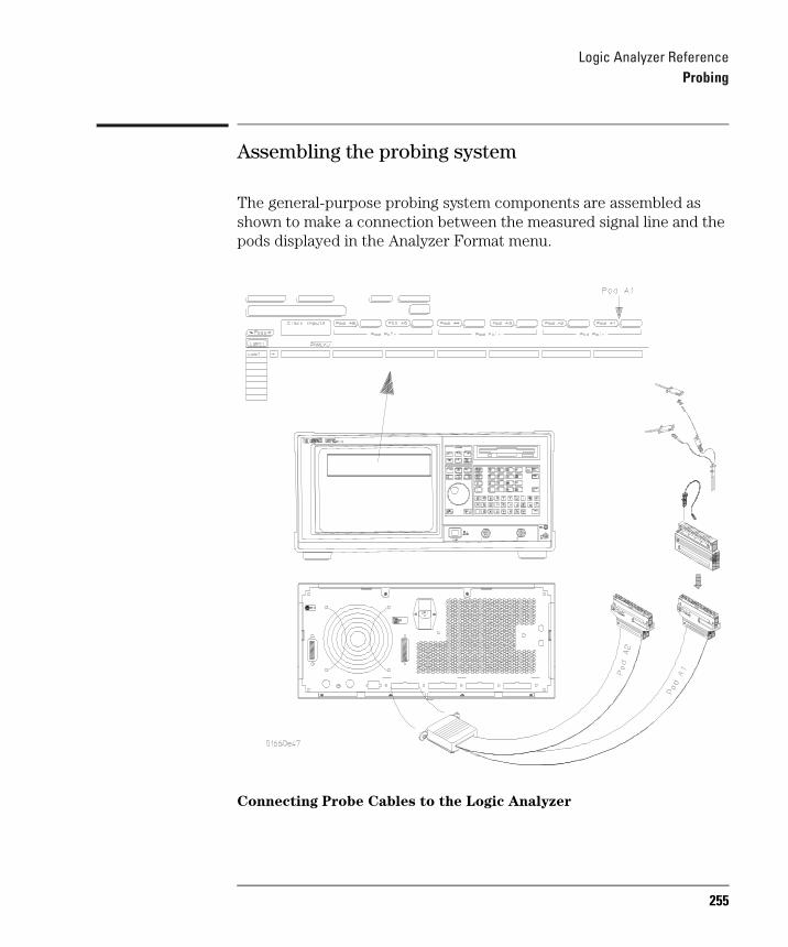
Logic Analyzer ReferenceProbing
Assembling the probing system
The general-purpose probing system components are assembled as shown to make a connection between the measured signal line and the pods displayed in the Analyzer Format menu.
Connecting Probe Cables to the Logic Analyzer
255
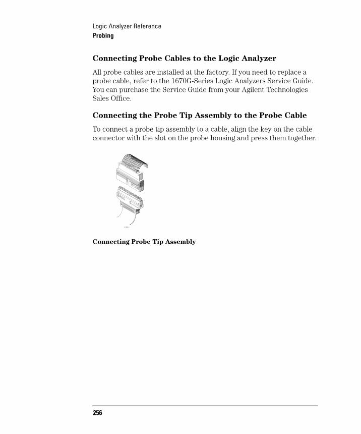
Logic Analyzer ReferenceProbing
Connecting Probe Cables to the Logic Analyzer
All probe cables are installed at the factory. If you need to replace a probe cable, refer to the 1670G-Series Logic Analyzers Service Guide. You can purchase the Service Guide from your Agilent Technologies Sales Office.
Connecting the Probe Tip Assembly to the Probe Cable
To connect a probe tip assembly to a cable, align the key on the cable connector with the slot on the probe housing and press them together.
Connecting Probe Tip Assembly
256
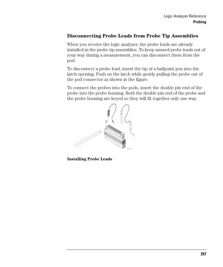
Logic Analyzer ReferenceProbing
Disconnecting Probe Leads from Probe Tip Assemblies
When you receive the logic analyzer, the probe leads are already installed in the probe tip assemblies. To keep unused probe leads out of your way during a measurement, you can disconnect them from the pod.
To disconnect a probe lead, insert the tip of a ballpoint pen into the latch opening. Push on the latch while gently pulling the probe out of the pod connector as shown in the figure.
To connect the probes into the pods, insert the double pin end of the probe into the probe housing. Both the double pin end of the probe and the probe housing are keyed so they will fit together only one way.
Installing Probe Leads
257
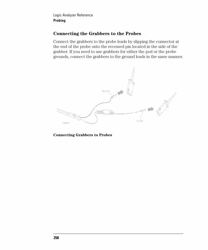
Logic Analyzer ReferenceProbing
Connecting the Grabbers to the Probes
Connect the grabbers to the probe leads by slipping the connector at the end of the probe onto the recessed pin located in the side of the grabber. If you need to use grabbers for either the pod or the probe grounds, connect the grabbers to the ground leads in the same manner.
Connecting Grabbers to Probes
258
Logic Analyzer ReferenceProbing
Oscilloscope probes (oscilloscope option only)
The two oscilloscope probes supplied with the oscilloscope option are Agilent Technologies 1160A Miniature Passive Probes. These small, lightweight probes allow measurements that were previously very difficult in densely populated circuits.
For complete information on the operation, maintenance, and adjustments of the miniature passive probes, be sure to read the operating note that is packaged with the probes.
Probe Inputs
Probe inputs are located on the front panel to the right of the power switch. Input 1 is on the left. The probes may be connected directly to the BNC input connectors. The signal is dc-coupled to the oscilloscope.
BNC cables can be connected directly to the BNC connectors. A BNC-to BNC cable is not provided with the instrument, but you can order it separately.
Maximum Probe Input Voltage
The maximum input voltage of each logic analyzer probe is ±40 volts peak. The maximum input voltage of the oscilloscope is ±250 volts dc at 1 MΩ setting and 5 volts rms at 50Ω setting.
Calibration Outputs
There is one calibration output BNC located on the rear panel. It is the AC/DC calibration signal source. This signal is used during calibration of the oscilloscope. This calibration signal can also be used for probe compensation adjustment.
259

Logic Analyzer ReferenceProbing
Connecting the pattern generator pods directly to a PC board (pattern generator option only)
To connect the pattern generator pods directly to the PC board, use one of the following two methods. Both methods require that a 3M 2520-series, or similar alternative connector be installed on the PC board.
Direct pod to board connection
Simply plug the pod directly into the 3M 2520-series, or similar alternative connector on the PC board.
Jumper cable to pod connection
Use this method when you have clearance problems on the PC board. Construct a flat ribbon cable and connect as shown below.
Equivalent connectors can be obtained from sources other than 3M.
260
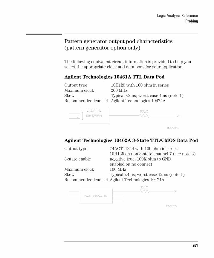
Logic Analyzer ReferenceProbing
Pattern generator output pod characteristics (pattern generator option only)
The following equivalent circuit information is provided to help you select the appropriate clock and data pods for your application.
Agilent Technologies 10461A TTL Data Pod
Output type 10H125 with 100 ohm in series Maximum clock 200 MHzSkew Typical <2 ns; worst case 4 ns (note 1)Recommended lead set Agilent Technologies 10474A
Agilent Technologies 10462A 3-State TTL/CMOS Data Pod
Output type 74ACT11244 with 100 ohm in series10H125 on non 3-state channel 7 (see note 2)
3-state enable negative true, 100K ohm to GNDenabled on no connect
Maximum clock 100 MHzSkew Typical <4 ns; worst case 12 ns (note 1)Recommended lead set Agilent Technologies 10474A
261

Logic Analyzer ReferenceProbing
Agilent Technologies 10464A ECL Data Pod (terminated)
Output type 10H115 with 330 ohm pulldown, 47 ohm in series
Maximum clock 200 MHzSkew Typical <1 ns; worst case 2 ns (see note 1)Recommended lead set Agilent Technologies 10474A
Agilent Technologies 10465A ECL Data Pod
(unterminated)
Output type 10H115 (no termination)Maximum clock 200 MHzSkew Typical <1 ns; worst case 2 ns (see note 1)Recommended lead set Agilent Technologies 10347A
262
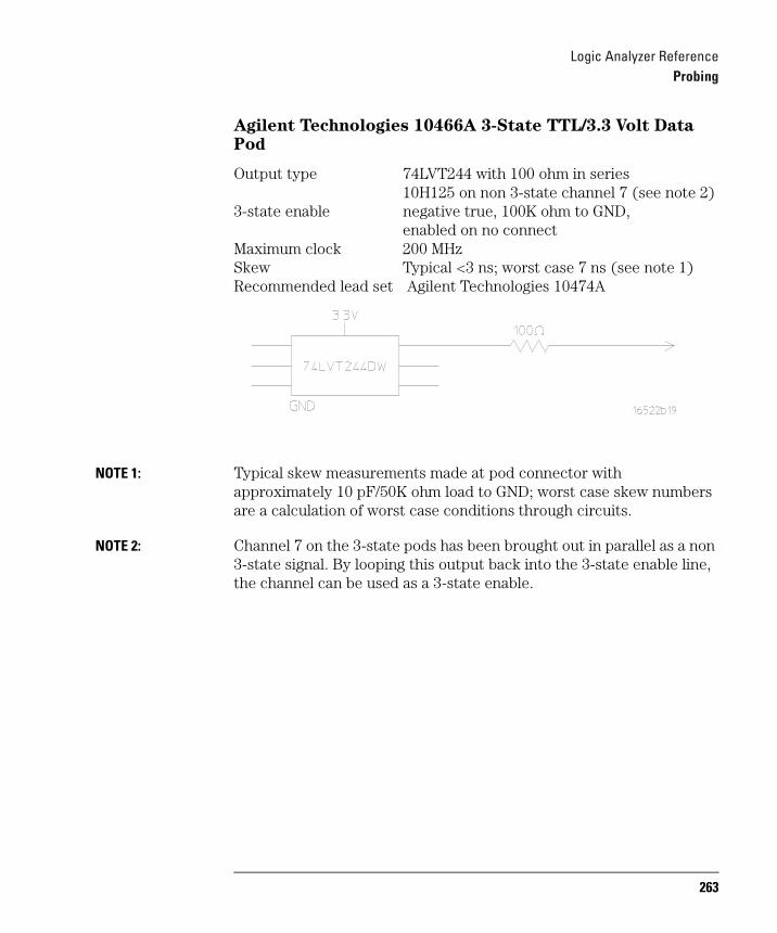
Logic Analyzer ReferenceProbing
Agilent Technologies 10466A 3-State TTL/3.3 Volt Data
Pod
Output type 74LVT244 with 100 ohm in series10H125 on non 3-state channel 7 (see note 2)
3-state enable negative true, 100K ohm to GND,enabled on no connect
Maximum clock 200 MHzSkew Typical <3 ns; worst case 7 ns (see note 1)Recommended lead set Agilent Technologies 10474A
NOTE 1: Typical skew measurements made at pod connector with approximately 10 pF/50K ohm load to GND; worst case skew numbers are a calculation of worst case conditions through circuits.
NOTE 2: Channel 7 on the 3-state pods has been brought out in parallel as a non 3-state signal. By looping this output back into the 3-state enable line, the channel can be used as a 3-state enable.
263

Logic Analyzer ReferenceProbing
Data Cable Characteristics Without a Data Pod
The 1670G-series, with the pattern generator option, data cables without a data pod provide an ECL-terminated (1 KW to -5.2 V) differential signal. These are usable when received by a differential receiver, preferably with a 100-ohm termination across the lines. These signals should not be used single ended due to the slow fall time and shifted voltage threshold (they are not ECL compatible).
264
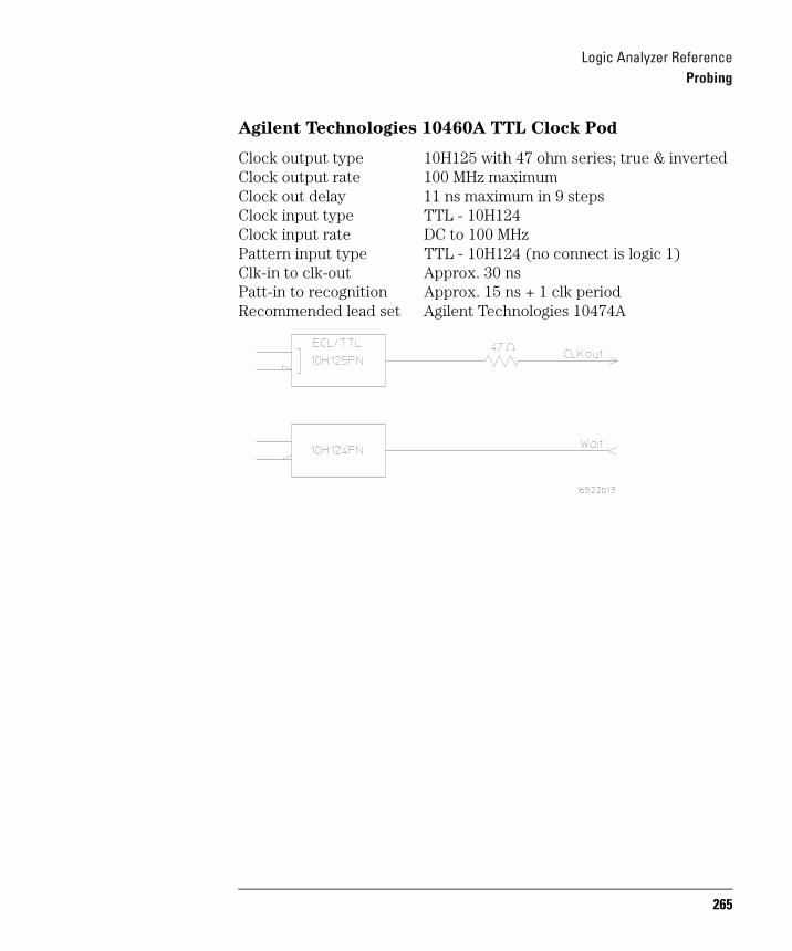
Logic Analyzer ReferenceProbing
Agilent Technologies 10460A TTL Clock Pod
Clock output type 10H125 with 47 ohm series; true & invertedClock output rate 100 MHz maximumClock out delay 11 ns maximum in 9 stepsClock input type TTL - 10H124Clock input rate DC to 100 MHzPattern input type TTL - 10H124 (no connect is logic 1)Clk-in to clk-out Approx. 30 nsPatt-in to recognition Approx. 15 ns + 1 clk periodRecommended lead set Agilent Technologies 10474A
265
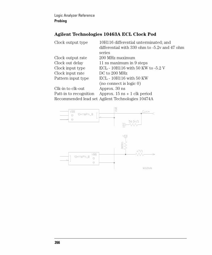
Logic Analyzer ReferenceProbing
Agilent Technologies 10463A ECL Clock Pod
Clock output type 10H116 differential unterminated; anddifferential with 330 ohm to -5.2v and 47 ohmseries
Clock output rate 200 MHz maximumClock out delay 11 ns maximum in 9 stepsClock input type ECL - 10H116 with 50 KW to -5.2 VClock input rate DC to 200 MHzPattern input type ECL - 10H116 with 50 KW
(no connect is logic 0)Clk-in to clk-out Approx. 30 nsPatt-in to recognition Approx. 15 ns + 1 clk periodRecommended lead set Agilent Technologies 10474A
266
Logic Analyzer ReferenceKeyboard Shortcuts
Keyboard ShortcutsThis section explains how to use the optional keyboard interface (Agilent Technologies E2427B Keyboard Kit). You can use the keyboard interchangeably with the knob and front-panel keypad for all menu applications. The keyboard functions fall into the two basic categories of cursor movement and data entry.
Moving the cursor
The keyboard cursor is the location on the screen highlighted in inverse video. Move the cursor using one of the methods described below.
Keyboard cursor movement
There are four cursor keys marked with arrows on the keyboard. These keys act as follows:
• Up-pointing arrow moves the cursor up.
• Down-pointing arrow moves the cursor down.
• Right-pointing arrow moves the cursor to the right.
• Left-pointing arrow moves the cursor to the left.
The cursor keys do not wrap. This means that pressing the right-pointing arrow when the cursor is already at the rightmost point in a menu will have no effect. The cursor keys do repeat, so holding the key down is the fastest way to continue keyboard cursor movement in a given direction.
267
Logic Analyzer ReferenceKeyboard Shortcuts
Page Up and Page Down keys
The Page Up and Page Down keys page through listings. The Page Up key displays the previous page of data. The Page Down key displays the next page of data.
Selecting a menu item
To select a menu item with the keyboard, position the cursor (the location highlighted in inverse video) on the menu item and press the Return or Enter key.
Entering data into a menu
When an assignment field is selected, the cursor is displayed under the leftmost character in the field. When you type a character, it is displayed in the cursor position, and the cursor is advanced. Cursor keys move the cursor within the assignment field. Pressing either the Return key or the Enter key will terminate data entry for that item.
268

Logic Analyzer ReferenceKeyboard Shortcuts
Using the keyboard overlays
A keyboard overlay is included in the E2427B Keyboard Kit. The table below represents the key mappings.
Key Functions Like Key Functions Like
F1 System Key S Select "seconds"
F2 Config Key M Select "milliseconds" or "millivolts"
F3 Format Key U Select "microseconds"
F4 Trigger Key N Select "nanoseconds"
F5 Listing Key V Select "volts"
F6 Waveform Key B Select "any (both) edge"
F7 Print All Key R Select "rising edge"
F8 Run Key F Select "falling edge"
F9 Stop * Assign glitch
F10 Done . Assign Don't Care (X)
F12 Assign Don't Care (X)
269

Logic Analyzer ReferenceCommon Menu Fields
Common Menu FieldsThere are a number of fields that appear throughout the different menus that have similar operation. These common fields are listed below:
• Mode (System/Analyzer) field
• Menu field
• Print field
• Run field
• Base field
• Label field
• Roll fields
Because most of these fields are self-explanatory, only the fields with less obvious features are described here.
270
Logic Analyzer ReferenceCommon Menu Fields
Print field
The Print field prints what is displayed on the screen at the time you initiate the printout. When you select the Print field, a print selection pop-up appears showing you one or more of the following options:
• Print Screen
• Print Disk
• Print All
• Print Partial
• Cancel
While printing, the Print field changes to Cancel and the user interface is not active except for Cancel. When the printout is complete, the user interface becomes active again. The Print field is not available with pop-up menus. The only way to print a pop-up menu to disk is with a controller.
Print Screen
The Print Screen option sends the screen immediately to the specified printer. The option does not create a file; to do that, use Print Disk.
271
Logic Analyzer ReferenceCommon Menu Fields
Print Disk
The Print Disk option copies the screen in graphical form or ASCII, if available, to a file on either drive. Possible output formats are
• ASCII 8-bit standard ASCII text file
• B/W TIF Black-and-white image in TIFF version 5.0 format
• Color TIF Color image in TIFF version 5.0 format
• PCX Color image in standard PCX format
• EPS Line image in standard Encapsulated PostScript format
Print All
The Print All option prints not only what is displayed on the screen, but data that is below the screen. This option is only available when an ASCII form of the screen is possible. For example, Print All is never available in Waveform.
When you select Print All with a Listing menu, make sure the first line you want to print is in the state location box (also referred to as the data roll field) at the center of the listing area. Lines above this box will not print.
Print Partial
The Print Partial option is identical to the Print All option, except the start and end states are specified. The screen settings and specified data are printed in ASCII form.
272
Logic Analyzer ReferenceCommon Menu Fields
Run/Stop field
The Run field starts the analyzer measurement. When you select Run, the screen switches to the display menu last viewed and displays the acquired data. If Stop is selected during a single run, the data acquisition is aborted. If Stop is selected during a repetitive run, the current run cycle is completed before data is displayed.
Repetitive
The Repetitive option runs the data acquisition cycle repeatedly until you select Stop or until a pre-assigned stop measurement condition is met. The stop measurement condition is set in the Analyzer Listing or Analyzer Waveform menus when pattern markers are turned on.
273
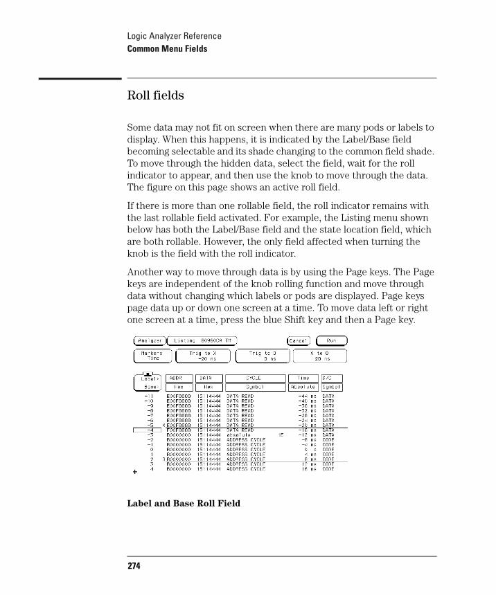
Logic Analyzer ReferenceCommon Menu Fields
Roll fields
Some data may not fit on screen when there are many pods or labels to display. When this happens, it is indicated by the Label/Base field becoming selectable and its shade changing to the common field shade. To move through the hidden data, select the field, wait for the roll indicator to appear, and then use the knob to move through the data. The figure on this page shows an active roll field.
If there is more than one rollable field, the roll indicator remains with the last rollable field activated. For example, the Listing menu shown below has both the Label/Base field and the state location field, which are both rollable. However, the only field affected when turning the knob is the field with the roll indicator.
Another way to move through data is by using the Page keys. The Page keys are independent of the knob rolling function and move through data without changing which labels or pods are displayed. Page keys page data up or down one screen at a time. To move data left or right one screen at a time, press the blue Shift key and then a Page key.
Label and Base Roll Field
274
Logic Analyzer ReferenceDisk Drive Operations
Disk Drive OperationsThe logic analyzer has a built-in 3.5-inch, double-sided, high-density or double-density, flexible disk drive. The disk drive is compatible with both LIF (Logical Interchange Format) and DOS (Disk Operating System) formats. It also has an internal hard disk drive, which performs the same operations as the flexible disk drive.
Disk operations
Ten disk operations are available:
• Autoload
Designates a set of configuration files to be loaded automatically the next time the analyzer is turned on.
• Copy
Copies files. Any file can be copied from one drive to another, from one directory to another, or to different flexible disks.
• Duplicate Disk
Copies one flexible disk to another flexible disk. You cannot copy the hard disk to a flexible disk in a single operation. All volume labels, directories, and file positions from one disk are copied exactly to another disk. The new disk is formatted to match the source disk if it is required. All files on the destination disk will be destroyed with this operation.
275
Logic Analyzer ReferenceDisk Drive Operations
• Format Disk
Formats a flexible disk or the internal hard disk. Either can be formatted in LIF or DOS format. All files on the disk will be destroyed with this operation.
• Load
Loads a file into the logic analyzer, overwriting the current settings or information. You can load system configurations, analyzer measurement setups including measurement data, and inverse assembler files.
• Make Directory
Creates a new directory on a DOS disk. You can save or copy files to the new directory using the store and copy commands. This is not available with LIF disks.
• Pack Disk
Removes all empty or unused sectors between files on a LIF disk so that more space is available. If you select Pack Disk while a DOS disk is in the drive, nothing happens.
• Purge
Purges (deletes) the file you indicate. Deleted files cannot be recovered.
• Rename
Changes the name of the file you select.
276
Logic Analyzer ReferenceDisk Drive Operations
• Store
Saves system and analyzer measurement setups including data.
Disk operation safeguards
If there is a problem or additional information is needed to execute an operation, a pop-up appears near the center of the screen displaying the status of the operation.
If executing a disk operation could destroy or damage a file, a pop-up appears when you select Execute. If you do not want to complete the operation, select Cancel to cancel the operation. Otherwise, select Continue.
277
Logic Analyzer ReferenceDisk Drive Operations
Autoload
The Autoload operation allows you to designate a set of configuration files to be loaded automatically the next time the analyzer is turned on. This allows you to change the default configuration of certain features to one that better fits your needs. If both the hard drive and flexible drive have autoload setups, only the setup on the flexible drive will be used.
Autoload loads all of the files for a given base filename. If you want to load only one type of file, rename that file or copy it to a separate name and enable it as the current Autoload file. As long as Autoload is enabled before the instrument is shut off, Autoload will remain enabled when you turn on the instrument and load the configuration files.
Format
CAUTION: Executing Format Disk permanently erases all existing information from the disk. After formatting, there is no way to retrieve the original information.
The logic analyzer recognizes a variety of sector sizes for LIF disks. However, it only creates 1024-byte sectors when formatting a LIF disk. DOS disks always have 512-byte sectors.
The logic analyzer does not support track sparing during formatting. If a bad track is found, the disk is considered bad. If a disk has been formatted elsewhere with track sparing, it will be read successfully.
When formatting a disk, the DISK ERROR message appears if the disk is unformatted. This is normal, and you can safely continue the format process.
278
Logic Analyzer ReferenceDisk Drive Operations
Pack
By purging files from the disk and adding other files, you may end up with blank areas on the disk (between files) that are too small for the new files you are creating. On LIF disks, the Pack Disk operation packs the current files together, removing unused areas from between the files so that more space is available for files at the end of the disk. On DOS disks, the Pack Disk operation is not available. If you do select Pack Disk while a DOS disk is in the drive, the disk is not affected.
279
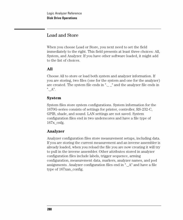
Logic Analyzer ReferenceDisk Drive Operations
Load and Store
When you choose Load or Store, you next need to set the field immediately to the right. This field presents at least three choices: All, System, and Analyzer. If you have other software loaded, it might add to the list of choices.
All
Choose All to store or load both system and analyzer information. If you are storing, two files (one for the system and one for the analyzer) are created. The system file ends in "._ _" and the analyzer file ends in "._A".
System
System files store system configurations. System information for the 1670G-series consists of settings for printer, controller, RS-232-C, GPIB, shade, and sound. LAN settings are not saved. System configuration files end in two underscores and have a file type of 167x_cnfg.
Analyzer
Analyzer configuration files store measurement setups, including data. If you are storing the current measurement and an inverse assembler is already loaded, when you reload the file you are now creating it will try to pull in the inverse assembler. Other attributes stored in analyzer configuration files include labels, trigger sequence, arming configuration, measurement data, markers, analyzer names, and pod assignments. Analyzer configuration files end in "._A" and have a file type of 167xan_config.
280
Logic Analyzer ReferenceDisk Drive Operations
Oscilloscope (oscilloscope option only)
Oscilloscope configuration files store measurement setups, including data. Attributes stored in scope configuration files include labels, trigger sequence, arming configuration, measurement data, markers, and channel assignments. Oscilloscope configuration files end in “._B” and have a file type of 167Xsc_config.
Pattern Generator (pattern generator option only)
Pattern generator files store the configuration attributes and parameters of the pattern generator, including vectors and functions, labels, pod assignments, and clock frequency. Pattern generator configuration files end in "._B" and have a file type of 16522_config.
281
Logic Analyzer ReferenceThe RS-232-C, GPIB, and Centronics Interfaces
The RS-232-C, GPIB, and Centronics InterfacesThis section describes the default setup, controller and printer interfaces and their configurations found in the System External I/O menu. It defines the GPIB interface and describes how to select a different GPIB address. It also defines the RS-232-C interface and tells you how to select a baud rate, how to change the stop bits, how to set the parity and data bits, and how to change the flow control protocol. The Centronics (parallel) interface (for printers only) and LAN interface (controller only) are also described.
Default Setup
Default Setup resets the logic analyzer to all the default settings. This gives you the same result as when you re-power the logic analyzer.
Controller interface
The logic analyzer is equipped with standard RS-232-C, GPIB, and Ethernet LAN interfaces that allow you to connect to a controller. All of the interfaces give you remote access for running measurements and uploading and downloading configurations and data.
Printer interface
The logic analyzer can output its screen to various GPIB, RS-232-C, and Centronics graphics printers. Configured menus, as well as waveforms and other data, can be printed for complete measurement documentation. The analyzer cannot use a networked or shared printer.
See Also "Connecting Peripherals" on page 36 for more details on physically connecting equipment.
Agilent Technologies 1670G-Series Logic Analyzers Programmer's Guide for more information on the controller interface.
The LAN section of this book on page 476 more information on the LAN interface.
282

Logic Analyzer ReferenceThe RS-232-C, GPIB, and Centronics Interfaces
The GPIB interface
The General Purpose Interface Bus (GPIB) is Agilent Technologies' implementation of IEEE Standard 488-1978, "Standard Digital Interface for Programmable Instrumentation." GPIB is a carefully defined interface that simplifies the integration of various instruments and computers into systems.
The GPIB interface uses an addressing technique to ensure that each device on the bus (interconnected by GPIB cables) receives only the data intended for it. To accomplish this, each device is set to a different address and this address is used to communicate with other devices on the bus. The GPIB address is the only GPIB interface setting configurable from the logic analyzer.
The GPIB address can be set to 31 different GPIB addresses, from 0 to 30. Simply choose a compatible address for your device and software. The default address for all Agilent logic analyzers is 7. In the System External I/O menu, select GPIB Settings and then set the Address field to your address.
283

Logic Analyzer ReferenceThe RS-232-C, GPIB, and Centronics Interfaces
The RS-232-C interface
The RS-232-C interface is Agilent Technologies' implementation of EIA Recommended Standard RS-232-C, "Interface Between Data Terminal Equipment and Data Communications Equipment Employing Serial Binary Data Interchange."
With this interface, data is sent one bit at a time and characters are not synchronized with preceding or subsequent data characters. Each character is sent as a complete entity independent of other events.
The paragraphs below describe the settings for RS-232-C. You can change these settings by going to the System External I/O menu and selecting RS232 Settings. Each field in the Settings pop-up menu presents a list of valid choices.
Baud rate
The baud rate is the rate at which bits are transferred between the interface and the peripheral. The baud rate must be set to transmit and receive at the same rate as the peripheral.
Stop Bits
Stop Bits are used to identify the end of a character. The number of Stop Bits must be the same for the controller as for the logic analyzer.
Parity
The parity bit detects errors as incoming characters are received. If the parity bit does not match the expected value, the character was incorrectly received. The action taken when an error is detected depends on the interface and the device program configuration.
Parity is determined by the requirements of the system. The parity bit may be included or omitted from each character by enabling or disabling the parity function.
284
Logic Analyzer ReferenceThe RS-232-C, GPIB, and Centronics Interfaces
Data Bits
Data Bits are the number of bits used to represent the binary code of a character. The 1670G-series logic analyzers, with the pattern generator, support 8-bit binary code.
Protocol
Protocol governs the flow of data between the instrument and the external device. It can be controlled either by the hardware, in which case you select None in the RS-232-C Settings pop-up, or by the software, in which case you select Xon/Xoff. Xon/Xoff stands for Transmit On/Transmit Off.
With less than a 5-wire interface, selecting None does not allow the sending or receiving device to control how fast the data is being sent, increasing the possibility of missing data. With a full 5-wire interface, selecting None allows a hardware handshake to occur. With a hardware handshake, hardware signals control data flow. The HP 13242G cable allows the logic analyzer to support hardware handshake.
The Centronics interface
The Centronics interface is an industry-standard parallel printer interface. It can only be used as a printer interface, and is not available to the controller. There are no Centronics-specific settings; page and line length are set in the Printer Settings menu.
See Also "Connecting Peripherals" on page 36 for more information on setting up the parallel printer port.
285
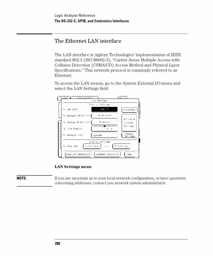
Logic Analyzer ReferenceThe RS-232-C, GPIB, and Centronics Interfaces
The Ethernet LAN interface
The LAN interface is Agilent Technologies’ implementation of IEEE standard 802.3 (ISO 88002-3), “Carrier Sense Multiple Access with Collision Detection (CSMA/CD) Access Method and Physical Layer Specifications.” This network protocol is commonly referred to as Ethernet.
To access the LAN menus, go to the System External I/O menu and select the LAN Settings field.
LAN Settings menu
NOTE: If you are uncertain as to your local network configuration, or have questions concerning addresses, contact you network system administrator.
286
Logic Analyzer ReferenceThe RS-232-C, GPIB, and Centronics Interfaces
LAN Port
There are two ports for connecting the logic analyzer to LAN. The LAN TP port is for a twisted pair network, sometimes known as ethertwist or 10Base-T. The LAN BNC port is for a coaxial cable network, sometimes know as thinlan or 10Base2. The LAN Port field toggles between these two ports. Select the field that matches your LAN network and the back-panel connector you are using.
Analyzer IP Address
This is the IP address that the logic analyzer will respond to, and must be unique on the network. If you need to create and IP address, contact your system administrator. Enter the analyzer address in this field.
Gateway IP Address
The gateway IP address is only necessary if the host computer and logic analyzer are on different subnets. Use the address of the gateway nearest the logic analyzer between the analyzer and the host. Your system administrator should be able to provide this information.
File Timeout
The file timeout is the amount of time the logic analyzer will keep a file in memory. If you are transferring 1 M of data, the file timeout must be larger than if you are transferring 64 K of data. The file timeout can also affect the network timeout. Generally, 1.5 seconds is a good value.
Analyzer name
You can assign an analyzer name to the logic analyzer. It does not have to be the same as the IP alias, although you could set it to that. This name shows up in the X Window title bar and in ASCII files created by the analyzer.
287
Logic Analyzer ReferenceThe RS-232-C, GPIB, and Centronics Interfaces
Help with...
These buttons provide additional information on the LAN settings screen, hosts table, and PC settings.
Show LAN Connections
This field pops up a list of all connections to the logic analyzer, and some information as to the type of connection. An IP address followed by “0.0” is an X Window connection. A line beginning with FTP is an ftp PARSER SOCKET is a telnet connection. A straight IP address or computer name is an NFS client.
Ethernet Statistics
This field pops up a display showing the analyzer’s ether address, the subnet mask, and transmit and receive statistics on the current session, which may be helpful for troubleshooting. These fields are not configurable.
See Also The LAN section of this User’s Guide on page 476 for more details.
288
Logic Analyzer ReferenceSystem Utilities
System UtilitiesThe System Utilities menu is used for setting system level parameters such as the system clock, display intensity for each shade, and the sound. In this menu you can also rewrite the analyzer's memory with any new revisions of the operating system.
Real Time Clock Adjustments field
A real-time clock is displayed in the Waveform and Listing menus. When you print a screen, the current clock and date appear on the hard copy. To change the clock, go to the System Utilities menu and select Real Time Clock Adjustments. Set the values to the desired date and time.
The Time Zone field changes the logic analyzer's apparent file times when viewed over NFS. It does not affect the real-time clock. Set the Time Zone to the same Time Zone used by your LAN. This value is usually the same as the difference in hours between your local time and Greenwich Mean Time.
289
Logic Analyzer ReferenceSystem Utilities
Update FLASH ROM field
The logic analyzer uses flash ROMs to store the operating system. The analyzer you received should have an operating system in place and should also include the operating system files on a flexible disk, but you may occasionally need to update the operating system. Update FLASH ROM updates the analyzer's operating system.
CAUTION: Updating flash ROM without the proper files will damage the logic analyzer operating system.
1 Go to the System Utilities menu.
2 Select Update FLASH ROM.
The analyzer warns, "Selecting Continue Will Erase & Update Flash ROMs." and waits for you to select Cancel or Continue. If you select Continue, the analyzer will be reset. If you need to save the measurement data, select Cancel.
3 Select Continue.
The screen goes black and the analyzer performs its power-up self tests. It then displays a message listing the required files and provides further instructions.
4 Insert the update disk into the flexible disk drive.
5 To search only the flexible disk drive, press the Done key. To search the flexible disk drive and then the hard drive, press any other key.
290
Logic Analyzer ReferenceSystem Utilities
If you press a key other than Done, the logic analyzer will not pause for you to insert the second disk when it finishes copying files from the first disk. Instead, it will look on the hard drive under the /SYSTEM directory. If it finds copies of the operating system files on the hard drive, those are used instead. This could result in incorrect installation of the updated operating system.
The logic analyzer warns, "We are about to erase flash ROM memory." This is the last point at which you can cancel the operation. Any loss of power between the time the analyzer starts to erase flash ROM and the time it finishes copying the update will destroy the operating system.
CAUTION: If you do not have the required files, turn off the analyzer immediately. Pressing any key will destroy the operating system.
6 If you are sure you are ready to continue, press any key.
7 When the analyzer has completed the update, press any key.
The screen goes black and the analyzer reboots. You have finished updating the flash ROM and the new operating system is in place. It is now safe to turn off the logic analyzer.
291
Logic Analyzer ReferenceDisplay Color Selection
Display Color SelectionThe color selection feature allows you to customize display colors, which improves contrast and lessens eye fatigue caused by your operating environment. If you are color-blind to certain colors, are operating in a difficult light environment, or don't like the default colors, you can quickly and easily change them.
The colors used by an X Window are always the default colors, and cannot be changed.
The Color Model: Hue, Saturation, and Luminosity
The 1670G-series logic analyzers use the HSL color model (Hue, Saturation, and Luminosity). This model is very effective for interactive color selection. Similar in concept to the method used by artists for mixing paints, pure hues are selected, and then white and black are mixed to dilute the color or darken it.
• Hue is the pure color. 0 is red, 33 green, and 67 blue. The selection ranges from 0 to 100.
• Saturation is the ratio of the pure color mixed with white (0 to 100%).
• Luminosity is the brightness per unit area (0 to 100%).
The figure on the next page shows a cylindrical representation of the HSL model (Hue, Saturation, and Luminosity). Hue is the angular coordinate, Saturation is the radial coordinate, and Luminosity is the altitude above the polar coordinate plane.
The cylinder rests on a black plane (Luminosity = 0%) and extends upward. As you increase in altitude, you increase luminosity, which represents an increase in brightness. Whenever luminosity is zero, the values of saturation and hue do not matter. Zero luminosity is black, and 100% luminosity gives you the pure color.
292
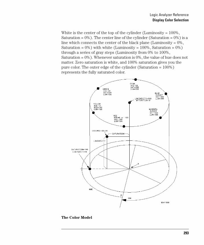
Logic Analyzer ReferenceDisplay Color Selection
White is the center of the top of the cylinder (Luminosity = 100%, Saturation = 0%). The center line of the cylinder (Saturation = 0%) is a line which connects the center of the black plane (Luminosity = 0%, Saturation = 0%) with white (Luminosity = 100%, Saturation = 0%) through a series of gray steps (Luminosity from 0% to 100%, Saturation = 0%). Whenever saturation is 0%, the value of hue does not matter. Zero saturation is white, and 100% saturation gives you the pure color. The outer edge of the cylinder (Saturation = 100%) represents the fully saturated color.
The Color Model
293
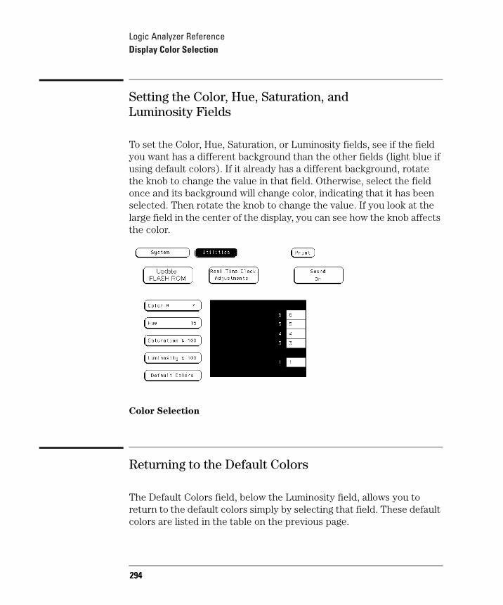
Logic Analyzer ReferenceDisplay Color Selection
Setting the Color, Hue, Saturation, and Luminosity Fields
To set the Color, Hue, Saturation, or Luminosity fields, see if the field you want has a different background than the other fields (light blue if using default colors). If it already has a different background, rotate the knob to change the value in that field. Otherwise, select the field once and its background will change color, indicating that it has been selected. Then rotate the knob to change the value. If you look at the large field in the center of the display, you can see how the knob affects the color.
Color Selection
Returning to the Default Colors
The Default Colors field, below the Luminosity field, allows you to return to the default colors simply by selecting that field. These default colors are listed in the table on the previous page.
294
Logic Analyzer ReferenceThe Analyzer Configuration Menu
The Analyzer Configuration Menu
Type field
The Type field lets you configure the logic analyzer with either an internal clock (Timing mode) or an external clock (State and SPA). When the Type field is selected, the following choices are available.
Timing. When Timing is selected, the analyzer uses its own internal clock to clock measurement data into the acquisition memory. This clock is asynchronous to the signals in the target system. Fields relating to external clocks such as the Analyzer Format menu's Master Clock do not appear and certain menus such as Compare are not available.
The analyzer can only be configured with one timing analyzer. If two are selected, the first will be turned off.
State. When State is selected, the analyzer uses a clock from the system under test to clock measurement data into acquisition memory. This clock is synchronous to the signals in the target system.
State Compare. When State Compare is selected, the Compare menu is available in the main menu selection. For more details on Compare, see “The Compare Menu.” State Compare mode functions much like State mode, except that total memory is reduced.
SPA. SPA stands for System Performance Analysis. It uses an external clock like a state analyzer but measures overall system performance rather than recording discrete activity. For more details on SPA, see page 350.
295
Logic Analyzer ReferenceThe Analyzer Configuration Menu
Illegal configuration
When both analyzers are turned on, the first pod pair 1,2 and the last pod pair cannot be assigned to the same analyzer machine. If this configuration is set, the analyzer will display a re-assignment menu when you try to leave the configuration screen. Use this re-assignment menu to configure the pod assignment automatically to a legal configuration.
296
Logic Analyzer ReferenceThe Analyzer Format Menu
The Analyzer Format Menu
Pod threshold field
The pod threshold field is used to set a voltage level that the data must reach before the analyzer recognizes and displays it as a change in logic levels. Threshold levels apply to single pods, and cover both data and clock channels.
TTL. When TTL is selected, the threshold level is +1.5 volts.
ECL. When ECL is selected, the threshold level is -1.3 volts.
User. When User is selected as the threshold level, the data signals must reach a user selectable value. The range of this value is between -6.0 volts to +6.0 volts in 50-mV increments.
297
Logic Analyzer ReferenceThe Analyzer Format Menu
State acquisition modes
The State Acquisition Mode field identifies the channel width and memory depth of the selected acquisition mode. There are two configurations of channel width/memory depth.
Full Channel/64K Memory/150 MHz
Full-channel mode uses both pods in a pod pair for 34 channels of width and a total memory depth of 64 K per channel. If time or state tags are turned on, the total memory is evenly split between data acquisition storage and time or state tag storage. To maintain the full 64 K per channel depth with state or time tags, leave one pod pair unassigned.
Half Channel/128K Memory/150 MHz
Half-channel mode cuts the channel width to 17 channels. In this mode, the pod used within the pod pair is selected through the Pod field. In half-channel mode, the memory depth is increased to 128 K per channel. Time or state tags are not available in this mode.
298
Logic Analyzer ReferenceThe Analyzer Format Menu
Timing acquisition modes
The Timing Acquisition mode field identifies the acquisition type, the channel width, and sampling speed of the present acquisition mode. There are three acquisition modes and five configurations.
Conventional Acquisition Mode
In Conventional Acquisition mode, the analyzer stores measurement data at each sampling interval.
299
Logic Analyzer ReferenceThe Analyzer Format Menu
Acquisition modes
The Acquisition mode field identifies the channel width and sampling speed of the present acquisition mode. There are two timing acquisition modes. State analyzers only have one acquisition mode.
Full-channel 250 MHz. Data is sampled and stored as often as every 4 ns.
Half-channel 500 MHz. Data is sampled and stored as often as every 2 ns, but only one of the pods in each pod pair is active.
150 MHz State. Data is synchronously sampled and stored.
See Also See page 92 for memory configurations.
“Configuration Capabilities” in this chapter and “Managing Memory”on page 89 for additional information on memory configurations.
300
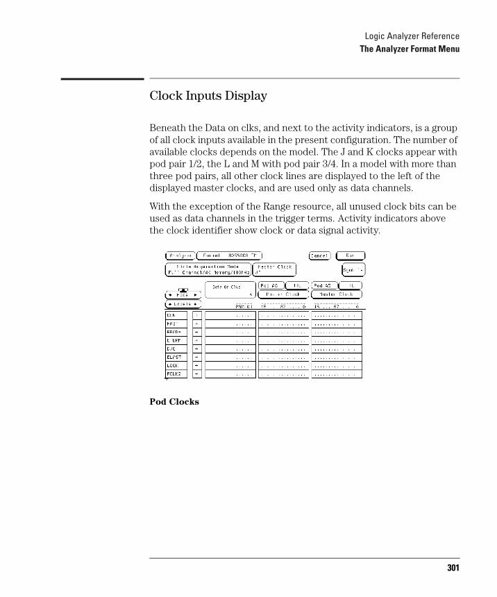
Logic Analyzer ReferenceThe Analyzer Format Menu
Clock Inputs Display
Beneath the Data on clks, and next to the activity indicators, is a group of all clock inputs available in the present configuration. The number of available clocks depends on the model. The J and K clocks appear with pod pair 1/2, the L and M with pod pair 3/4. In a model with more than three pod pairs, all other clock lines are displayed to the left of the displayed master clocks, and are used only as data channels.
With the exception of the Range resource, all unused clock bits can be used as data channels in the trigger terms. Activity indicators above the clock identifier show clock or data signal activity.
Pod Clocks
301
Logic Analyzer ReferenceThe Analyzer Format Menu
Pod clock field (State only)
The pod clock field identifies the type of clock arrangement assigned to each pod. When the pod clock field is selected, a clock arrangement menu appears with the choices of Master, Slave, or Demultiplex. Once a pod clock is assigned a clock arrangement, its identity and function follows what is configured in the Master and Slave Clock fields.
Master
This option specifies that data on all pods designated "Master Clock," in the same analyzer, are strobed into memory when the status of the clock lines match the clocking arrangement specified under the Master Clock.
See Also "Master and Slave Clock fields (State only)" found later in this section for information about configuring a clocking arrangement.
Slave
This option specifies that data on a pod designated "Slave Clock" is latched when the status of the slave clock meets the requirements of the slave clocking arrangement. Then, followed by a match of the master clock and the master clock arrangement, the slave data is strobed into analyzer memory along with the master data. See the figure on the following page.
If multiple slave clocks occur between master clocks, only the data latched by the last slave clock prior to the master clock is strobed into analyzer memory.
302

Logic Analyzer ReferenceThe Analyzer Format Menu
Latching Slave Data
Analyzer Memory
Slave Latch
latches on master clock
latches on slave clock
data on master data on slave
303
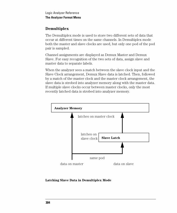
Logic Analyzer ReferenceThe Analyzer Format Menu
Demultiplex
The Demultiplex mode is used to store two different sets of data that occur at different times on the same channels. In Demultiplex mode both the master and slave clocks are used, but only one pod of the pod pair is sampled.
Channel assignments are displayed as Demux Master and Demux Slave. For easy recognition of the two sets of data, assign slave and master data to separate labels.
When the analyzer sees a match between the slave clock input and the Slave Clock arrangement, Demux Slave data is latched. Then, followed by a match of the master clock and the master clock arrangement, the slave data is strobed into analyzer memory along with the master data. If multiple slave clocks occur between master clocks, only the most recently latched data is strobed into analyzer memory.
Latching Slave Data in Demultiplex Mode
Analyzer Memory
Slave Latch
latches on master clock
latches on slave clock
data on master data on slave
same pod
304
Logic Analyzer ReferenceThe Analyzer Format Menu
Master and Slave Clock fields (State only)
The Master and Slave Clock fields are used to construct a clocking arrangement. A clocking arrangement is the assignment of appropriate clocks, clock edges, and clock qualifier levels which allow the analyzer to synchronize itself on valid data.
Clock selections
When the Master or Slave Clock field is selected, a clock/qualifier selection menu appears showing the available clocks and qualifiers for a clocking arrangement. Depending on the model, there are a maximum of four clocks available (J through M), and a maximum of four clock qualifiers available (Q1 through Q4).
Clock edges are ORed to clock edges, clock qualifiers are ANDed to clock edges, and clock qualifiers can be either ANDed or ORed together. All clock and qualifier combinations on the left side of the graphic line are ORed to all combinations on the right side of the line. For example, in a six-clock model, all combinations of the J, K, and L clock with Q1 and Q2 qualifiers, are ORed to the clock combinations of the M, N, and P clocks with Q3 and Q4 qualifiers.
305
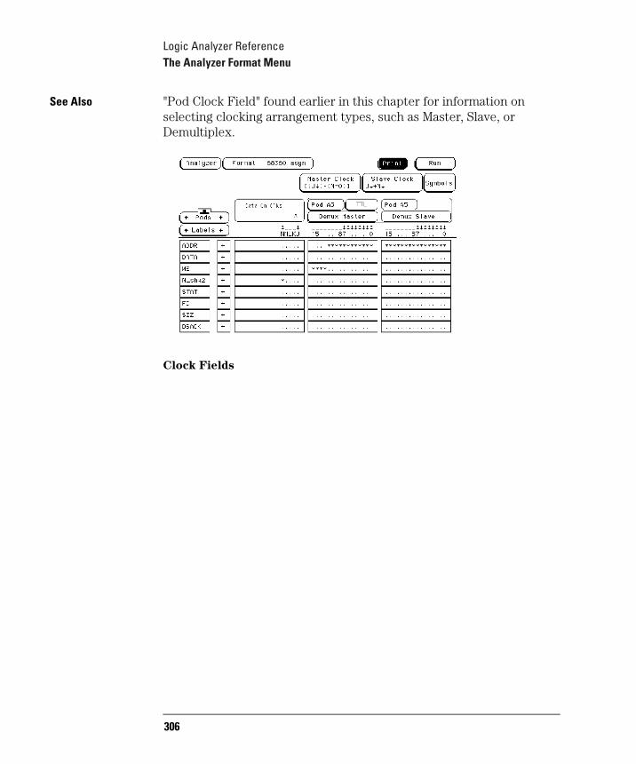
Logic Analyzer ReferenceThe Analyzer Format Menu
See Also "Pod Clock Field" found earlier in this chapter for information on selecting clocking arrangement types, such as Master, Slave, or Demultiplex.
Clock Fields
306
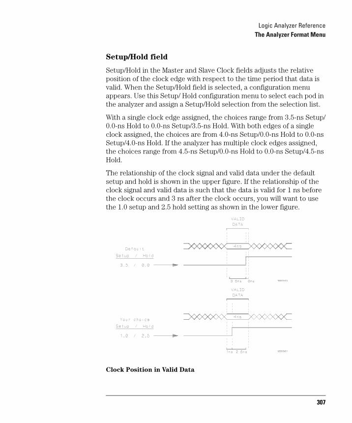
Logic Analyzer ReferenceThe Analyzer Format Menu
Setup/Hold field
Setup/Hold in the Master and Slave Clock fields adjusts the relative position of the clock edge with respect to the time period that data is valid. When the Setup/Hold field is selected, a configuration menu appears. Use this Setup/ Hold configuration menu to select each pod in the analyzer and assign a Setup/Hold selection from the selection list.
With a single clock edge assigned, the choices range from 3.5-ns Setup/0.0-ns Hold to 0.0-ns Setup/3.5-ns Hold. With both edges of a single clock assigned, the choices are from 4.0-ns Setup/0.0-ns Hold to 0.0-ns Setup/4.0-ns Hold. If the analyzer has multiple clock edges assigned, the choices range from 4.5-ns Setup/0.0-ns Hold to 0.0-ns Setup/4.5-ns Hold.
The relationship of the clock signal and valid data under the default setup and hold is shown in the upper figure. If the relationship of the clock signal and valid data is such that the data is valid for 1 ns before the clock occurs and 3 ns after the clock occurs, you will want to use the 1.0 setup and 2.5 hold setting as shown in the lower figure.
Clock Position in Valid Data
307
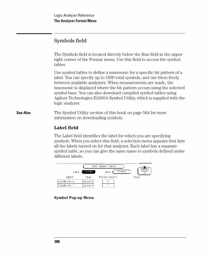
Logic Analyzer ReferenceThe Analyzer Format Menu
Symbols field
The Symbols field is located directly below the Run field in the upper right corner of the Format menu. Use this field to access the symbol tables.
Use symbol tables to define a mnemonic for a specific bit pattern of a label. You can specify up to 1000 total symbols, and use them freely between available analyzers. When measurements are made, the mnemonic is displayed where the bit pattern occurs using the selected symbol base. You can also download compiled symbol tables using Agilent Technologies E2450A Symbol Utility, which is supplied with the logic analyzer.
See Also The Symbol Utility section of this book on page 564 for more information on downloading symbols.
Label field
The Label field identifies the label for which you are specifying symbols. When you select this field, a selection menu appears that lists all the labels turned on for that analyzer. Each label has a separate symbol table, so you can give the same name to symbols defined under different labels.
Symbol Pop-up Menu
308
Logic Analyzer ReferenceThe Analyzer Format Menu
Base field
Use the Base field to select the numeric base in which the pattern in the symbols menu is displayed. Binary is not available if more than 20 channels are assigned to a label because there is only enough room for 20 bits to be displayed on the screen.
You cannot specify a pattern or range when the base is ASCII. Define the pattern or range in one of the other bases, then switch to ASCII to see the ASCII characters.
Symbol Width field
The Symbol Width field specifies how many characters of the symbol name will be displayed when the symbol is referenced in the Trigger, Waveform, and Listing menus. You can display from 1 to 16 characters of the symbol name.
Symbol name field
When you first access the symbol table, there are no symbols specified. The symbol name field reads "New symbol." Select this field to enter a symbol name. When you are done, a symbol Type field becomes active.
Type field
The symbol Type field toggles between pattern and range. When the symbol is defined as a pattern, a Pattern/Start field appears to the right of the Type field. To assign a pattern, select the Pattern/Start field and type in the desired pattern.
If the symbol is defined as a range, a Pattern/Start field and a Stop field appear. Use these fields to specify the upper and lower boundaries of the range. To assign values to the boundaries, select the fields and enter the pattern. You can specify ranges that overlap or are nested within each other.
309

Logic Analyzer ReferenceThe Analyzer Format Menu
Label fields
The label fields are the fields with label names along the left side of the display below the field captioned Labels. The default label names are Bus1 through Bus126. Selecting the label fields pops up a choice of Turn Label On, Turn Label Off, and Modify Label.
The Turn Label Off option turns off the label. When a label is turned off, the label name and the bit assignments are saved by the logic analyzer so that you can turn the label back on and not have to retype the bit assignments and name. With labels off, the label names remain displayed for identification and searching purposes. Turning labels off may save memory in transitional timing.
Labels may have from 1 to 32 channels assigned to them. If you try to assign more than 32 channels to a label, the logic analyzer will beep, indicating an error. A message will appear at the top of the screen telling you that 32 channels per label is the maximum.
Channels assigned to a label are numbered from right to left by the logic analyzer. The least significant assigned channel on the far right is numbered 0, the next assigned channel is numbered 1, and all other channels are assigned sequentially up to the maximum of 16 per pod. Because 32 channels can be assigned to one label at most, the highest number that can be given to a channel is 31.
Although labels can contain split fields, assigned channels are always numbered consecutively within a label.
310
Logic Analyzer ReferenceThe Analyzer Format Menu
Label polarity fields
The label polarity fields, which are located just after the label, are used to assign a polarity to each label. The default polarity for all labels is positive (+). You change the label polarity by toggling the polarity field.
When the polarity is positive, 1 is high and 0 is low. When the polarity is negative, 1 is low and 0 is high. All data as well as bit-pattern specific configurations used for identifying, triggering, or storing data reflect the change of polarity. Numbers use the appropriate logical encoding, but waveforms and edges are still shown as logic levels, either low or high. In a timing analyzer with the data inverted, the waveform display remains positive true.
As an example, setting the logic analyzer to trigger on 0A hex with positive polarity is the same as setting it to trigger on F5 hex with negative polarity. The listing would show 0A with + polarity, F5 with - polarity. In the waveform menu, if the waveform is defined as bus the waveform shown as symbols inverts with a change of polarity. If the waveform is defined as individual channels or is not using symbols, it is not affected by changing polarity.
311
Logic Analyzer ReferenceThe Analyzer Trigger Menu
The Analyzer Trigger Menu
Trigger sequence levels
Sequence levels are the definable stages of the total trigger specification. Individual sequence levels are assigned using either a predefined trigger function or a user-level trigger function. The total trigger specification can contain both kinds of function.
See Also "Using the Trigger Menu" on page 70 for more on setting up a trigger.
Sequence level usage
Generally, you would think using one function in one sequence level uses up one of the available sequence levels. This may not always be the case. Some of the more complex predefined functions require multiple sequence levels. Keep this point in mind if you are near the limit on remaining sequence levels. The exact number of internal levels required per function, and the remaining available levels, are shown within the function library list. User functions, however, use only one level almost all the time. The only instance where multiple levels are used with the User function is when the "<" duration is assigned.
312
Logic Analyzer ReferenceThe Analyzer Trigger Menu
Modify Trigger field
The Modify Trigger field allows you to modify the statements of any single sequence level as well as perform other high-level actions like global clearing of existing trigger statements, and adding or deleting sequence levels. Break Down Functions/Restore Functions acts a bit differently than the others.
Break Down Functions / Restore Functions
When a predefined function is broken down, the contents of that function are displayed in the same long form used in the User function. If the function uses multiple internal levels, all levels are separated out and displayed in the sequence levels of the Trigger menu. Once the functions in your trigger specification are broken down, Break Down Functions changes to Restore Functions. Use Restore Functions to restore all functions to their original structure.
When the function is in a broken-down form, you can change the structure. However, when the functions are restored, all changes are lost and any branching that is part of the original structure is restored.
Use Break Down Functions if you want to view a particular function part in its long form to see the exact sequence flow. Breaking down functions can also help in creating a custom trigger specification.
When a function is broken down, you have all the assignment fields and branching options available as though they were a set of User functions.
313

Logic Analyzer ReferenceThe Analyzer Trigger Menu
Timing trigger function library
The following list contains all the functions in the library of timing trigger functions. They are listed in the same order as they appear onscreen.
User Mode User level - custom combinations, loops
The User level is a user-definable level. This level offers low-level configuration and uses one internal sequence level. If the "<" duration is used, four levels are required.
Basic Functions 1. Find edge
This function becomes true when the designated edge is seen. It uses one internal sequence level.
2. Find Nth occurrence of an edge
This function becomes true when it finds the designated occurrence of a designated edge. It uses one internal sequence level.
3. Find pattern present/absent for > duration
This function becomes true when it finds a designated pattern that has been present or absent for greater than or equal to the set duration. It uses one internal sequence level.
4. Find pattern present/absent for < duration
This function becomes true when it finds a designated pattern that has been present or absent for less than the set duration. It uses four or five internal sequence levels.
5. Find anystate "n" times
This function becomes true when the first state it sees occurs "n" number of times. It uses one internal sequence level.
314

Logic Analyzer ReferenceThe Analyzer Trigger Menu
Pattern/Edge 1. Find edge and pattern
Combinations This function becomes true when a selected edge type is seen at the same time as a designated pattern. It uses one internal sequence level.
2. Find pattern occurring too soon after edge
This function becomes true when a designated pattern is seen occurring within a set duration after a selected edge type is seen. It uses three or four internal sequence levels.
3. Find pattern occurring too late after edge
This function becomes true when one selected edge type occurs, and for a designated period of time after that first edge is seen, a pattern is not seen. It uses two internal sequence levels.
Time Violations 1. Find 2 edges too close together
This function becomes true when a second selected edge is seen occurring within a designated period of time after the occurrence of a first selected edge. It uses three or four internal sequence levels.
2. Find 2 edges too far apart
This function becomes true when a second selected edge occurs beyond a designated period of time after the first selected edge. It uses two internal sequence levels.
3. Find width violation on a pattern/pulse
This function becomes true when the width of a pattern violates designated minimum and maximum width settings. It uses four or five internal sequence levels.
Delay • Wait "t" seconds
This function becomes true after a designated time period has expired. It uses one internal sequence level.
315
Logic Analyzer ReferenceThe Analyzer Trigger Menu
State trigger function library
The following list contains all the functions in the library of state trigger functions. They are listed in the same order as they appear onscreen.
User Mode User level - custom combinations, loops
The User level is a user-definable level. This level offers low-level configuration and uses one internal sequence level.
Basic Functions 1. Find event "n" times
This function becomes true when it sees a designated pattern occurring a designated number of times consecutively or nonconsecutively. It uses one internal sequence level.
2. Find event "n" consecutive times
This function becomes true when it sees a designated pattern occurring a designated number of consecutive times. It uses one internal sequence level.
3. Find event 2 immediately after event 1
This function becomes true when the first designated pattern is seen immediately followed by a second designated pattern. It uses two internal sequence levels.
4. Find anystate "n" times
This function becomes true when the first state it sees occurs "n" number of times. It uses one internal sequence level.
316
Logic Analyzer ReferenceThe Analyzer Trigger Menu
Sequence 1. Find event 2 "n" times after event 1 before event 3
occurs
Dependent functions This function becomes true when it first finds a designated pattern 1, followed by a selected number of occurrences of a designated pattern 2. In addition, if a designated pattern 3 is seen anytime while the sequence is not yet true, the sequence starts over. If pattern 2's "nth" occurrence is coincident with pattern 3, the sequence starts over. It uses two internal sequence levels.
2. Find too few states between event 1 and event 2
This function becomes true when a designated pattern 1 is seen, followed by a designated pattern 2, and with less than a selected number of states occurring between the two patterns. It uses three or four internal sequence levels.
3. Find too many states between event 1 and event 2
This function becomes true when a designated pattern 1 is seen, followed by at least a selected number of states, then followed by a designated pattern 2. It uses two internal sequence levels.
4. Find n-bit serial pattern
This function finds an "n" bit serial pattern on a designated channel and a designated label. It uses "n" internal sequence levels.
Time Violations 1. Find event 2 occurring too soon after event 1
This function becomes true when a designated pattern 1 is seen, followed by a designated pattern 2, and with less than a selected time period occurring between the two patterns. It uses two internal sequence levels.
2. Find event 2 occurring too late after event 1
This function becomes true when a designated pattern 1 is seen, followed by at least a selected time period, before a designated pattern 2 occurs. It uses two internal sequence levels.
317
Logic Analyzer ReferenceThe Analyzer Trigger Menu
Delay 1. Wait "n" external clock states
This function becomes true after a designated number of user clock states have occurred. It uses one internal sequence level.
318

Logic Analyzer ReferenceThe Analyzer Trigger Menu
Modifying the user function
Before you begin building a trigger specification using the user function, it should be noted that in most cases one of the predefined trigger functions will work.
If you need to accommodate a specific trigger condition, or you prefer to construct a trigger specification from scratch, use the User function as a starting point. This function appears in long form, which means it has the analyzer's total flexibility available in terms of resource terms, global timers, occurrence counters, duration counters, and two-way branching.
The User function has a "fill-in-the-blanks" type statement. You have the following elements to use:
• Bit Patterns, Ranges, and Edges
• Storage Qualification
• < and > Durations
• Occurrence Counters
• Timers
• Branching
A typical method used during a debug operation is to first trigger on a known pattern, edge or range. From that point, it becomes an iterative process of adding more levels to further filter the data. It is important for you to know how to use such elements as occurrence counters, timers, and branching, to zero in and trigger at the desired point.
319
Logic Analyzer ReferenceThe Analyzer Trigger Menu
As the analyzer executes the trigger specification, it searches for a match between the resource term value and the data. When a match is found, that part of the sequence statement becomes true and the sequencing continues to the next part of the statement or the next sequence level.
Eventually a path of "true" resource terms leads to your trigger command. If timers or occurrence counters are used, the analyzer waits or counts occurrences of a specified value before continuing.
The following examples illustrate the use of resource terms, occurrence counters, timers, branching, and store qualification. You will use them in your trigger specification either by themselves or combined with each other.
Using bit patterns, ranges, and edges
Bit patterns are set to match specific data values, and ranges are set to match a range of bit patterns. In the Timing Acquisition mode, edges are set to match specific edges of a timing pulse.
Using storage qualification
Store qualification lets you store all data, no data, or just selected data, before trigger occurs.
Setting < and > durations (Timing only)
When a resource term is found during a timing sequence evaluation, you can dictate how long the term must remain before it actually becomes true. When less than (<) or greater than (>) duration is assigned, the secondary branching (Else on) is not available.
> field. When greater than (>) is used, the analyzer continues sequence level evaluation only after the resource term has been true for greater than or equal to the amount of duration specified.
< field. When less than (<) is used, the analyzer continues sequence level evaluation only after the resource term has been true for less than or equal to the amount of duration specified. Using less than requires four sequence levels.
320
Logic Analyzer ReferenceThe Analyzer Trigger Menu
Using the Occurrence Counters
Occurs field. When "Occurs" is selected, the < and > duration functions change to an occurrence counter. Use the occurrence counter to delay sequence evaluation until the resource term has occurred a designated number of times. If the "else on" branch becomes true before all specified occurrences of the primary "Trigger on" branch, the secondary "else on" branch is taken.
Using the timer
Timers are like other resource terms in that they are either true or false. Timers can be set to Start, Stop, Pause, or Continue as the analyzer enters a sequence level. The two timers are global, so each sequence level can control the same timer. The default timer condition in all sequence levels is Off.
Timers start as you enter the sequence level, and when the timer count expires, the timer becomes true. If a timer is paused in one level, it must be continued in another level before it can count through.
As more sequence levels are added, the timer status in the new levels defaults to Off. Timers must be continued or started in each new level as appropriate. When a timer expires or stops, its count resets to zero.
Branching
If either the less than or greater than duration is used, only the primary branch is available. Otherwise, each sequence level except for the last has two-way branching.
If the primary branch is taken, the analyzer goes to the next level. If the primary branch is not found, the analyzer immediately evaluates the "Else on" secondary branching term.
321
Logic Analyzer ReferenceThe Analyzer Trigger Menu
If the "Else on" term is found, the secondary branch taken is to the designated sequence level. If the "Else on" term is not found, the analyzer continues to loop within the same sequence level until one of the two branches is found. If the "Else on" branch is taken, the occurrence counter is reset even if the "go to level" branch is back to the same level. If both branches are found true at the same time, the primary branch is taken.
Branching across the trigger level is possible. If this occurs, the sequence level evaluation could loop without ever seeing a trigger term. Be careful in designing your sequence instructions.
322
Logic Analyzer ReferenceThe Analyzer Trigger Menu
Resource terms
Resource terms are user-defined variables that are assigned to sequence levels. They are placed into the sequence statement where their bit pattern or edge type is searched for within the data stream. When a match is found, a branch is initiated and the next statement or sequence level is acted upon. Resource terms take the following forms:
• Bit pattern terms a-j
• Range terms 1 and 2
• Edge terms 1 and 2 (Timing only)
• Global timers 1 and 2
All resource terms and timer terms are listed in a scrollable Terms field. To view all offscreen terms, select the Terms field, then use the knob to roll the terms list onscreen.
When the logic analyzer is configured as a state analyzer, you can use any of the ten bit pattern terms, range terms, or timers in your trigger specification. When you configure the logic analyzer as a timing analyzer, you can use any of these terms plus the edge terms.
Bit pattern terms a-j
You can set a bit pattern consisting of any combination of 1s, 0s, or Xs (don't cares) for the 10 terms a ƒ j. Bit pattern terms can also take the NOT form of a - j.
Range terms 1 and 2
Two range terms are available which can be set to a range of bit pattern values. The first pattern and the last pattern are part of the range which must be matched.
Range terms take the form of either In Range, or the NOT form of Out Range.
323

Logic Analyzer ReferenceThe Analyzer Trigger Menu
Edge terms 1 and 2 (Timing only)
The two edge terms are only available in the timing analyzer. Each edge term is assigned positive-going, negative-going, or any-transition edge type, or glitch.
Global timers 1 and 2
In addition to the resource terms available, there are two global timers available. Each timer can be started, paused, continued, or stopped from any sequence level except the first.
Assigning resource term names and values
The Terms field identifies the list of available resource terms within the analyzer. A resource term can be assigned to only one machine at a time. The resource term names (a - j, Edge1, Edge2, Range1, Range2) are default names that can be changed. You assign values in the following two ways:
• Using Preset Values
• Assigning Bit by Bit
Changing resource properties. When any of the individual term fields are selected, a configuration pop-up menu appears. Use this pop-up menu to quickly set the resource term to a preset value.
324

Logic Analyzer ReferenceThe Analyzer Trigger Menu
Using Preset Values
Assign. Assign toggles which machine the term is assigned to. All of the available resource terms except the Edge terms can be assigned to any analyzer. However, a term can only be assigned to one analyzer at a time.
Rename. Rename lets you change the term name. This function works for all terms.
Clear (=X). Clear sets the terms to their broadest possible meaning. For terms a - j, the assignment field is set to all Xs (don't cares). For Range 1 and 2, the boundaries are set to the maximum and minimum values. For Timers 1 and 2, the assignment field is set to a minimum time of 400 ns. For Edge 1 and 2, the assignment field is set to don't cares.
Set (=1). In terms a - j, the assignment field is set to its maximum value, with all bits set to 1. This option is not available for the Range, Timer, and Edge terms.
Reset (=0). In terms a - j, the assignment field is set to its minimum value, with all bits set to 0. This option is not available for the Range, Timer, and Edge terms.
Assigning Bit by Bit
Bit pattern terms. Just to the right of the bit pattern name fields are the term assignment fields. When any of the individual assignment fields are selected, a keypad appears. Use this keypad to assign real values or Don't Care (X) values.
Edge terms. Assign edge terms the same way you do bit pattern terms. Edge terms can be used singularly or in combination with each other across all assigned channels. When you specify an edge on more than one channel, the analyzer ORs the edges.
325
Logic Analyzer ReferenceThe Analyzer Trigger Menu
After the assignment menu closes, you may see "$" indicators in the field display. A "$" indicates the assignment can't be displayed in the selected base because of Don't Cares. When you display the assignment in binary, however, you can see the actual pattern.
Range terms. Range terms require an upper and lower bit pattern boundary. The range is recognized as the data that is numerically between or on the two specified boundaries. In addition, the range must be contained in a single label across a single pod pair, with no clock bits allowed.
Timer terms. Timers are either true or false. Timers start as you enter the sequence level, and when the count expires, the it becomes true. If a timer is paused in one level, it must be continued in another level before it can count through.
As more sequence levels are added, the timer status in the new levels defaults to Off. Timers must be continued or started in each new level if it is appropriate. When a timer expires or stops, its count resets to zero.
Combination of terms
Combination terms are configured and selected from within trigger sequence levels. All user-defined resource terms can be combined to create complex qualifiers that occupy a single assignment field space.
When you select the term field in a Sequence Level menu, a pop-up selection list appears. If you then select "Combination," a logical assignment menu appears. Use this menu to turn on resource terms and input them into a chain of logical operators.
When the combination is placed in the assignment field, if the term is too long to fit in the assignment field, the display is truncated.
326

Logic Analyzer ReferenceThe Analyzer Trigger Menu
Arming Control field
Arming Control sets up the order of triggering for complicated measurements involving more than one machine. You can set the logic analyzer to begin running when it receives a signal from an external machine, have one analyzer start the other, or have one analyzer send a signal to another external machine. The default configuration has both analyzers running independently without external communications.
Arming control between analyzers
If both analyzers are turned on, you can configure one analyzer to arm the other. When you select the analyzer name in the Arming Control menu, a pop-up menu for selecting where the Arm In signal is coming from appears. This pop-up menu also selects the sequence level in which an "arm" flag is placed.
When an analyzer receives an Arm In signal, the arm term in the user-selected sequence level becomes true. If the analyzer was waiting at a trigger sequence level for the arm term, the analyzer begins evaluating the rest of that sequence level. However, if the arm term is not part of the current sequence level, the preceding sequencing could trigger the analyzer before the arm term is seen. Generally, the arm term is evaluated and used the same as the other resource terms within the sequence instruction.
Arming control using external BNCs
A more complex arming example involves passing arm signals in and out through the External BNCs on the rear panel. In the Arming Control menu, the External Triggers are called "Port In" and "Port Out". “PORT IN” can be selected in the Arming Control menu for the analyzer, scope or pattern generator, and “PORT OUT” can be selected in the Port Out key for the modules.
327
Logic Analyzer ReferenceThe Analyzer Trigger Menu
One possible scenario is to have several test instruments and a logic analyzer connected to a complex target system. The analyzer is armed by an external Arm In signal from another test/measurement entity. After the first analyzer triggers, it arms the second analyzer. After the second analyzer triggers, it sends a Port Out signal through the external BNC. This signal is used to arm another external test/measurement entity.
The Arm Out signal can be generated by either one of the two local analyzers.
328

Logic Analyzer ReferenceThe Analyzer Trigger Menu
Acquisition Control field
Selecting the Acquisition Control field pops up the Acquisition Control menu. The Acquisition Control menu sets the acquisition mode, the trigger position within acquisition memory, and the sample period.
Acquisition Mode field
The Acquisition Mode field toggles between Manual and Automatic. When set to Automatic, the position of stored data relative to trigger and the sample rate are based on the sec/Div and delay settings in the Waveform menu.
When Acquisition Mode is set to Manual, additional configuration fields become available. The additional configuration fields work together with the sequence instructions in a prioritized manner to position the memory relative to the trigger point. A small picture at the bottom of the menu displays the sum effect of all the settings on the trigger position within memory.
Memory Length
The Memory Length field set the amount of memory to be used for acquisition. It applies to all acquisition modes. Only discrete sizes are available (see “To set the memory length” on page 91). If you enter a number with the keyboard, it is rounded to the nearest available discrete size.
Trigger Position field
The Trigger Position field sets how much information is stored before and after the trigger. When a run is started, a timing analyzer will not look for a trigger until at least the proper percent of pre-trigger data has been stored. A state analyzer will trigger at the first occurrence of the trigger, but will notify you that the prestore was not completed. After a trigger has been detected, the rest of memory is filled before the analyzer halts.
329
Logic Analyzer ReferenceThe Analyzer Trigger Menu
In a timing analyzer, even when the trigger position is set to Start or End, there will always be a small portion of pre-trigger and post-trigger data stored. Most of the choices designate prestore and poststore percentages, but the Delay setting affects when the memory begins storing data relative to the trigger.
Delay (Timing only)
The Delay field delays the start of acquisition storage after the trigger. The delay time range is affected by the sample period but could range from 16 ns to 8 ks. As the picture in the pop-up menu shows, any data falling between the trigger and the delay time is not stored.
Branches Taken Stored / Not Stored field
The Branches Taken field is a toggle field that sets the analyzer to store, or not to store, the resource term that sent the analyzer off on a branch.
As the analyzer steps through the sequence instructions, it may take either branch of a sequence level. With Branches Taken set to Stored, the state data values that caused the branch are stored. When the analyzer is set to Branches Taken Not Stored, only the data you explicitly designate in the sequence levels is stored.
The Branches Taken Stored/Not Stored is not available when the analyzer is configured as a timing analyzer.
330
Logic Analyzer ReferenceThe Analyzer Trigger Menu
Count field (State only)
The Count field accesses a selection menu which indicates whether acquisition data is stamped with a Time tag or a State Count tag.
Time and State tags
If you have all pod pairs assigned, the state acquisition memory is reduced by half when time or state tags are turned on. You can maintain full memory depth if you leave a specified pod pair unassigned.
States. States places numbered tags on all data relative to the trigger. Pre-trigger data has negative numbers and post-trigger data has positive. In the display menus, State numbering is either relative to the previous memory location or absolute from the trigger point. You can set it in the display menus by toggling the Absolute/Relative field.
Time. Count time places time tags on all displayed data. Data stored before triggering has negative time numbers and data stored after triggering has positive time numbers. Time tag numbering is set to be either relative to the previous memory location or absolute from the trigger point. Selecting the Absolute or Relative option is done by toggling the Absolute/Relative field. Time tag resolution is 8 ns.
To retain full memory using time or state tags. To retain full memory depth when using time or state tags requires that one pod pair be unassigned. The exact pair to unassign varies. Generally, it is best to unassign one of the middle pod pairs. If you have two analyzers configured, the ends must be assigned to different analyzers.
331
Logic Analyzer ReferenceThe Listing Menu
The Listing Menu
Markers
The Markers field accesses the markers selection menu. When the Markers field is selected, a marker selection menu appears with the marker choices appropriate for the present analyzer configuration.
Off
The Off selection turns off marker operations but does not turn off operations based on the markers. For example, if a stop measurement was previously specified and the stop measurement criteria are met, the measurement will stop even though the markers are off.
Pattern markers
Pattern markers identify and mark unique bit patterns in the data listing. Once the unique bit patterns are marked, you can use them as reference points or as criteria for a stop measurement.
When a marker is positioned in the Listing menu, it is also positioned in the Chart menu and Waveform menu, but not in the Mixed Display menu.
State analyzer markers
In a state analyzer with Count Off in the Trigger menu, only Pattern markers are available. With Count Time turned on, Time markers and Statistics markers become available. With Count States turned on, State markers become available.
332
Logic Analyzer ReferenceThe Listing Menu
Timing analyzer markers
Timing analyzers always have marker choices of Pattern, Time, or Statistics. Timing analyzers do not have state markers. The pattern markers, though, can be used to count intervening patterns.
Stop measurement field
The stop measurement function specifies a condition that stops the analyzer measurement during a repetitive run. If two analyzers are configured, both analyzers stop when either specified stop condition is satisfied.
Off . The Off selection turns all Stop measurement operations off. If the stop measurement operation is not turned off and the stop measurement criteria is met, the measurement will stop even though the markers are set to other types or turned off.
X-O. The X-O option is available in the Timing analyzer and in the State analyzer with its count set to Time.
When X-O is selected, a repetitive run is stopped when a comparison of the time period between the X and O markers and one of the time period options is true.
Compare. When you select Compare, a repetitive run is stopped when a comparison of data in the Listing menu and data and criteria in the Reference listing of the Compare menu matches an equality selection. The equality selection is set from the Equal/Not Equal selection pop-up menu.
Statistics markers
After patterns are assigned to the X and O markers, statistical information is available when markers are set to Statistics.
In a State analyzer, Statistics markers only become available when the Trigger menu Count field is set to Time.
Statistics are based on the time between the X and O. Both markers must be found before valid statistical information is displayed.
333
Logic Analyzer ReferenceThe Waveform Menu
The Waveform Menu
sec/Div field
When acquisition control is set to automatic, the sec/Div field affects the sample period. Timing waveforms are reconstructed relative to the sample period. A shorter sample period puts more sample points on the waveform for a more accurate reconstruction but also fills memory more quickly.
If the sec/Div is changed resulting in a change in the next sample period, you must run the analyzer again before the current sample period display is updated. The sample period is shown in the second row from the top when the markers are turned off.
Accumulate field
The Accumulate field controls whether old data is cleared or displayed along with new data. The Accumulate field will toggle On/Off. When Accumulate is on, the analyzer displays the data from a current acquisition on top of the previously acquired data. When Accumulate is off, the display is cleared before each new run cycle.
If you leave the Waveform menu, or pop up a menu over the waveform display, any accumulated display data is lost and the accumulation process starts over.
334
Logic Analyzer ReferenceThe Waveform Menu
Delay field
Depending on the analyzer configuration, a positive or negative delay measured in either states (State only) or time (Timing only) can be set. The Delay field lets you scroll the data and place the display window at center screen. Changing the delay will not affect the data acquisition unless it is a timing analyzer and the acquisition mode is automatic. In this case, the sample period changes.
The delay range of a timing analyzer is from -2500 seconds to +2500 seconds. The delay range of a state analyzer is dependent on memory length and cannot exceed total memory size.
Waveform label field
The waveform label field, located on the left side of the waveform display, is both a display and configuration field. After all desired waveforms are configured for display, they are listed in the waveform label field. If there are more waveforms than can be displayed, you can roll the list by selecting the waveform label field, then after the roll indicator appears, turn the knob.
If the waveform label field is selected a second time, a waveform modification menu appears. Use this menu to configure the waveform display.
When the waveform modification menu appears, select the operation to insert, replace, delete, or scale waveforms into the display. You can display a maximum of 24 waveforms on screen at one time.
335
Logic Analyzer ReferenceThe Waveform Menu
Viewing state values in the bus option
When all assigned waveforms in a label are overlaid with the Bus option, the value of the data is displayed in the base selected in the Listing menu to the right of each new transition in the waveform display. This happens only when the waveform size is set to large.
If the sec/Div is set to view a large increment of time, or the waveform scaling is set to small or medium, the state data readout does not fit between transitions. To display the state data readouts within the waveform, expand the sec/Div and use the large waveform setting.
336
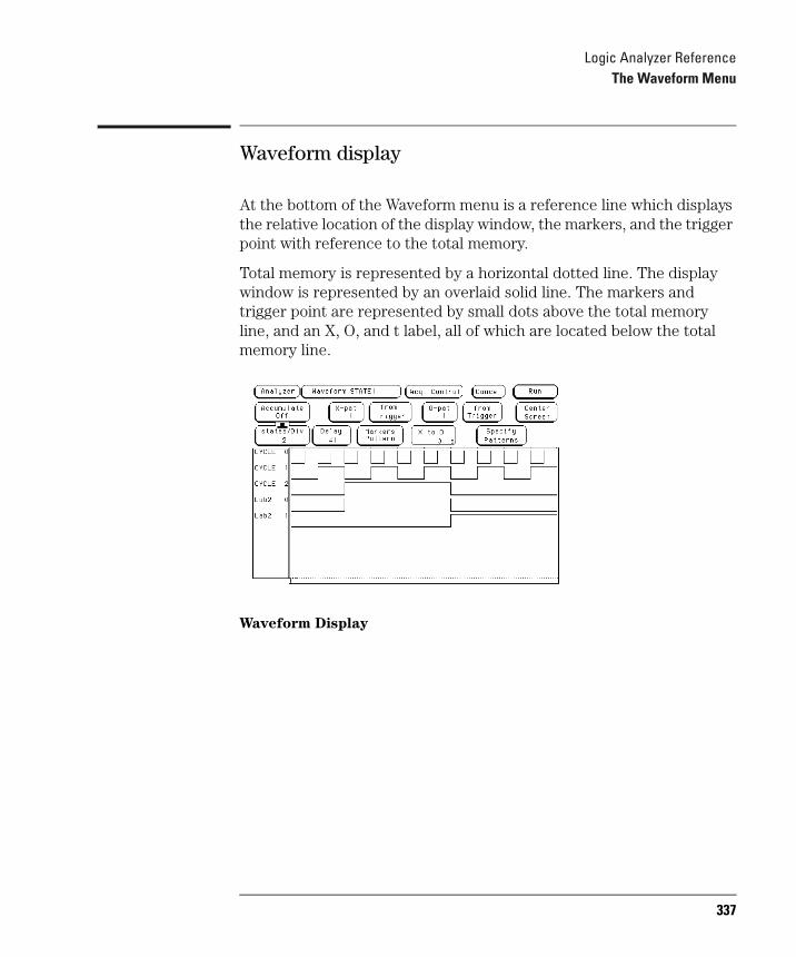
Logic Analyzer ReferenceThe Waveform Menu
Waveform display
At the bottom of the Waveform menu is a reference line which displays the relative location of the display window, the markers, and the trigger point with reference to the total memory.
Total memory is represented by a horizontal dotted line. The display window is represented by an overlaid solid line. The markers and trigger point are represented by small dots above the total memory line, and an X, O, and t label, all of which are located below the total memory line.
Waveform Display
337
Logic Analyzer ReferenceThe Mixed Display Menu
The Mixed Display MenuThe Mixed Display menu combines a state listing display located at the top of the menu and a waveform display located at the bottom of the menu. The Mixed Display menu shows both state and timing data in the same display.
The Mixed Display menu only becomes available when at least one analyzer is configured as a state analyzer, with its Count field in the Trigger menu set to Time. If two state analyzers are configured, both state listing displays can be interleaved as well as shown separately, however, the listing menus are the best display menus for a two-state analyzer configuration.
The waveform display area shows timing analyzer waveforms from the configured timing analyzer, the oscilloscope waveform (analyzers with the oscilloscope option), or both.
Interleaving state listings
Interleaved state listings lets you view two labels and their data from different analyzers in the same column. The process of interleaving state listings can be performed in either the Listing menu or the Mixed Display menu. For example, if data is interleaved in the Listing menu, it will be automatically interleaved in the Mixed Display menu.
The interleaved label is placed directly above the selected label, and all interleaved data is displayed in yellow. In addition, the state numbers of the interleaved data are indented to the right. Because of the lack of room available in the listing portion of the Mixed Display menu, the label identifying the interleaved data is not displayed. For this reason, when two state analyzers are configured the listing menus should be used to display interleaved labels.
338

Logic Analyzer ReferenceThe Mixed Display Menu
Time-correlated displays
Once the Time markers are set in the Waveform display area of the Mixed Display menu, time-correlated X and O Time markers will be displayed in both the listing and the waveform display areas.
Markers
The markers in the Mixed Display menu are not the same as the markers in the individual Listing and Waveform menus. First, Mixed Display only has time markers. Second, markers placed in the individual waveform and listing menus will not transfer to the Mixed Display menu. You must place new Time markers on your points of interest in the Mixed Display.
339

Logic Analyzer ReferenceThe Chart Menu
The Chart MenuState Chart is a software post-processing feature that provides the ability to build x-y charts of label activity using state data. The Chart menu builds a graphical representation of the system under test. The Y axis always represents data values for a specified label. You can select whether the X axis represents states (rows in the state listing) or the data values for another label.
When the X-axis is set to State, X and O markers are available which display the current sample relative to the trace point and the corresponding Y-axis data value. Marker placement is synchronized with the normal state listing.
An accumulate mode is available that allows the chart display to build up over several runs.
You can generate x-y charts of Label vs. Label or Label vs. State.
Label vs. Label charts
When labels are assigned to both axes, the chart shows how the data acquired under one label varies relative to the other for a particular measurement. Label values are always plotted in ascending order from the bottom to the top of the chart and in ascending order from left to right across the chart. Plotting a label against itself will result in a diagonal line from the lower left to upper right corner. All markers are disabled when plotting this kind of chart.
Label vs. State charts
Label versus State is a plot of data values acquired under a label versus the memory location of the same data. The label value is plotted against successive memory location numbers.
340
Logic Analyzer ReferenceThe Chart Menu
Min and Max scaling fields
When State is selected for the X axis, the minimum and maximum values can range from -1 M to +1 M, depending on the trace point location.
When Label is selected for either axis, the minimum and maximum values range from 00000000 hex to FFFFFFFF hex regardless of the axis, because labels are restricted to 32 bits.
Markers/Range field
The Marker/Range field is a toggle field. If the field is set to Range, X and Y range fields become available to set the chart minimum and maximum range points. If the field is set to Markers, a marker selection menu appears with marker choices available with the present analyzer configuration.
In a state analyzer with Count Off in the Trigger menu, only Pattern markers are available. With Count Time on, Time markers and Statistics markers become available. With Count States on, States markers are available. The markers function just like those of the Waveform and Listing displays.
341
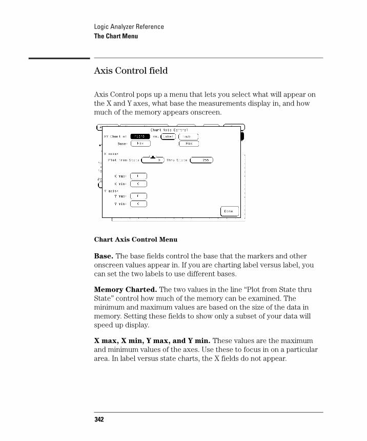
Logic Analyzer ReferenceThe Chart Menu
Axis Control field
Axis Control pops up a menu that lets you select what will appear on the X and Y axes, what base the measurements display in, and how much of the memory appears onscreen.
Chart Axis Control Menu
Base. The base fields control the base that the markers and other onscreen values appear in. If you are charting label versus label, you can set the two labels to use different bases.
Memory Charted. The two values in the line “Plot from State thru State” control how much of the memory can be examined. The minimum and maximum values are based on the size of the data in memory. Setting these fields to show only a subset of your data will speed up display.
X max, X min, Y max, and Y min. These values are the maximum and minimum values of the axes. Use these to focus in on a particular area. In label versus state charts, the X fields do not appear.
342

Logic Analyzer ReferenceThe Chart Menu
Rescale field
The Rescale field allows you to zoom in on a particular area, or move back to viewing the entire chart. To use Rescale, place your markers to box in an area you want to focus on, and then select one of the “between markers” choices. To move back to the big picture, choose Full Scale. You can also get a larger picture by setting the markers outside the current boundaries and choosing one of the “between markers” options.
When more data is available above or below the currently displayed data, “clip” is displayed just to the left of the corner of the display.
If you rescale the area between markers and you do not see your data, check the memory charted fields.
343

Logic Analyzer ReferenceThe Compare Menu
The Compare MenuState Compare is a software postprocessing feature that compares bit-by-bit the acquired state data listing and a reference listing. State Compare is only available when at least one analyzer is configured as a State analyzer.
The comparison between the acquired state listing data and the data in the reference listing is done relative to the trigger points. This means that the two data records are aligned at the trigger points and then compared bit-by-bit.
Any bits in the acquired data that do not match the bits in the compare image are treated as unequal.
You can separately view the acquired data, the reference listing, and a listing that highlights the bits in the acquired data that do not match the corresponding bits in the reference listing.
You can edit the reference listing for unique comparisons.
You can mask specific bits that you do not want to compare. These "Don't compare" bits can be specified individually for a given label and state row, or specified by channel across all state rows.
You can select a range of states to compare. When a range is selected, only the bits in states on or between the specified boundaries are compared. Also, you can save the reference listing along with the analyzer configuration to disk.
344
Logic Analyzer ReferenceThe Compare Menu
Reference Listing field
The Reference Listing field is a toggle field that switches the listing type between the Reference image listing and the Difference listing.
The Reference listing is a display of the image (or template) that acquired data is compared to during a comparison measurement. The boundaries of the image (or size of the template) are controlled by using the channel masking and compare range functions. Any bits in the reference listing displayed as "X" have been set to don't care bits during bit editing.
When the data listing is rolled, the difference data listing and the data listing in the Listing menu are also rolled.
Difference Listing field
The Difference Listing field is a toggle field that switches the listing type between the Reference image listing and the Difference listing.
The Difference listing is a display of the acquired data listing with the data that differs, if any, from the Reference listing, highlighted with inverse video. If the base is inverse assembled symbols, the entire line is highlighted with inverse video.
The controls that roll the listing in all three menus (the normal State listing, the Reference listing, and the Difference listing) are synchronized unless the number of pre-trigger states differ between the Reference listing and the acquired data.
345

Logic Analyzer ReferenceThe Compare Menu
This means that when you change the current row position in the Difference listing, the analyzer automatically updates the current row in the acquired State listing and Reference listing, and vice-versa.
If the three listings are synchronized and you acquire data again, the Reference listing may have a different number of pre-trigger states depending on the trigger criteria. The Reference listing can be resynchronized to the State and Difference listings by entering the desired state (acquisition memory) location from the front-panel keypad.
This lets you view corresponding areas of all lists, to cross check alignment, and to analyze the bits that do not match.
Copy Listing to Reference field
The initial Reference image is generated by either copying the data listing from the listing menu or by loading an analyzer configuration file which contains a Reference listing. Be aware that if you load an analyzer configuration to get a Reference image, the other menu setups will change.
When the Copy Listing to Reference field is selected, the contents of the acquisition data structure (Listing menu display) are copied to the Reference image buffer. The previous Reference image is lost if it has not been saved to a disk.
346
Logic Analyzer ReferenceThe Compare Menu
Find Error field
The Find Error field lets you easily locate any patterns that do not match in the current comparison. Occurrences of differences or errors are found in numerical ascending order from the start of the listing. The first occurrence of an error has the numerical value of one.
You select which error number to find by highlighting the Find Error field and entering a number from the front-panel keypad. If the roll indicator is in the Find Error field, simply turn the knob. The listing is then scanned sequentially until the specified occurrence is found and rolled into view.
Compare Full/Compare Partial field
The Compare Full/Compare Partial field is a toggle field which lets you compare either the full range of states or define a subset of the total number of states in the Reference image to be used in the comparison.
The Compare mode is accessed by selecting the Compare Full/Compare Partial field in either the Compare or Difference listing menus. When selected, a pop-up appears in which you select either the Full or Partial option.
When you select the Partial option, fields appear for setting the start state and stop state values. Only bits in states (lines) on or between the boundaries are compared against the acquired data.
347
Logic Analyzer ReferenceThe Compare Menu
Mask field
The channel masking field is used to specify a bit, or bits in each label that you do not want compared. This causes the corresponding bits in all states to be ignored in the comparison. The Reference data image itself remains unchanged on the display.
When you select the Mask field an assignment pop-up appears in which you specify which channels are to be compared and which channels are to be masked. A "." (period) indicates a don't compare mask for that channel and an "*" (asterisk) indicates that channel is to be compared.
Bit Editing field
The bit editing fields are located in the center of the Reference listing display. A bit editing field exists for every label in the display unless the label's base is ASCII or inverse assembled symbols. The bit editing field lets you modify the values of individual bits in the Reference image or specify them as don't compare bits.
You access data in the Reference listing by rolling the data listing using the knob until the data is located in the bit editing field. To enter a desired pattern or don't compare (X) for a bit, select the field and use the front-panel keypad.
348
10
System Performance Analysis (SPA) Software
349

System Performance Analysis (SPA) SoftwareSystem Performance Analysis Software
System Performance Analysis SoftwareThe System Performance Analysis (SPA) software is included as standard software in the 1670G-series logic analyzers.
SPA provides you with a set of functions for performing statistical analysis on your target system. Its functions include State Overview, State Histogram, and Time Interval modes.
To be successful with this software, you should be familiar with the operation of the logic analyzer.
This chapter is organized as follows:
• "What is System Performance Analysis?" outlines typical SPA applications, and describes the operating characteristics for each SPA mode.
• "Getting started" describes how to access the SPA menus and how to select the SPA modes and set the specifications.
• "SPA measurement processes" is a detailed description of the measurement processes used by the SPA package. This theory of operation explains how the SPA software samples and sorts the data from the target system, and how the onscreen measurement values are computed for the State Overview, State Histogram, and Time Interval modes.
• State Overview, State Histogram, and Time Interval" leads you through the State Overview, State Histogram, and Time Interval modes. It also tells how to set up SPA for the three modes, how to interpret the acquired data, and how to make measurements on specific areas of interest.
• "Using SPA with other features" tells you how to use SPA with other features.
350

System Performance Analysis (SPA) SoftwareSystem Performance Analysis Software
Error messages and warnings used by SPA are the same as those used by each of the logic analyzers. Refer to page 421 for descriptions of these messages.
If you need programming information, refer to the Agilent Technologies 1670G Series Logic Analyzers Programmer’s Guide. It is available from your Agilent Technologies Sales Office.
351
System Performance Analysis (SPA) SoftwareSystem Performance Analysis Software
What is System Performance Analysis?
The logic analyzer's state or timing analyzer is used to make quantitative measurements on specific events in the target system. For example, they can measure a specific time interval on a microprocessor's control lines or can find out how a particular subroutine was called.
System Performance Analysis, on the other hand, is used for qualitative measurements on the target system. SPA provides statistical analysis functions so you can determine how efficiently your target system is operating.
SPA repeatedly samples signals of interest, such as an address bus or the output of a counter. The multiple data sets from the repeated sampling are then used to build histograms and compile statistics that describe your target system's performance over time.
Some typical examples of SPA applications include:
• Obtain an overview of system activity.
• Identify software problems that lock up the microprocessor.
• Determine the best-case and worst-case execution times for a software module or a state machine.
• Establish standards for software modules or state machines.
• Identify inefficient use of mass storage and other peripherals.
• Evaluate memory utilization, such as illegal access in protected portions of memory, and locality of execution.
352
System Performance Analysis (SPA) SoftwareSystem Performance Analysis Software
Operating characteristics
The following describes the operating characteristics of the System Performance Analysis software for the three SPA measurement modes.
State Overview
The State Overview mode displays a bar chart of a label's state value versus the relative number of occurrences of each value in the defined range of the label. State Overview is available on any label defined in the Format Specification.
• The X axis is the defined range for the specified label which is divided into 256 buckets.
• The range of the specified label is user-definable.
• The Y axis is the relative number of occurrences in each bucket.
• The maximum value of the Y axis is constantly updated to reflect the number of occurrences in the bucket that has the most occurrences, and is displayed as "Max count".
• The total number of states sampled for the selected label is presented as Total count. This includes states that may be outside the user-specified Xaxis range.
• Two markers are available on the X axis to determine the range of a bucket and number of occurrences in any bucket.
• Choice of base for a specified label is user-definable.
353
System Performance Analysis (SPA) SoftwareSystem Performance Analysis Software
State Histogram
The State Histogram mode displays states that occur within user-defined ranges of a label. State Histogram is available on any label defined in the Format Specification.
• The maximum number of ranges is 11.
• Other States included/excluded is available and displays a histogram of all states not covered by the user-defined ranges.
• You can trace All States or patterned Qualified States.
• Total samples displays the total number of occurrences in all displayed ranges.
• The choice of base for specified label is user-definable.
Time Interval
The Time Interval mode displays time intervals between user-defined start and end events.
• Start and end events can be defined over all labels defined in the Format Specification.
• 10 ns is the minimum sample period and time interval resolution.
• The maximum number of time interval ranges is 8.
• The time interval range size is 10 ns to 9,999,999 seconds.
• Calculated statistics provides Maximum time, Minimum time, Average time, and Total number of time intervals sampled (one time interval defined to be a paired start/end event).
• The auto-range feature automatically scales the eight time intervals over maximum and minimum times using a logarithmic scale or linear scale.
• Choice of base for labels is user-definable.
354
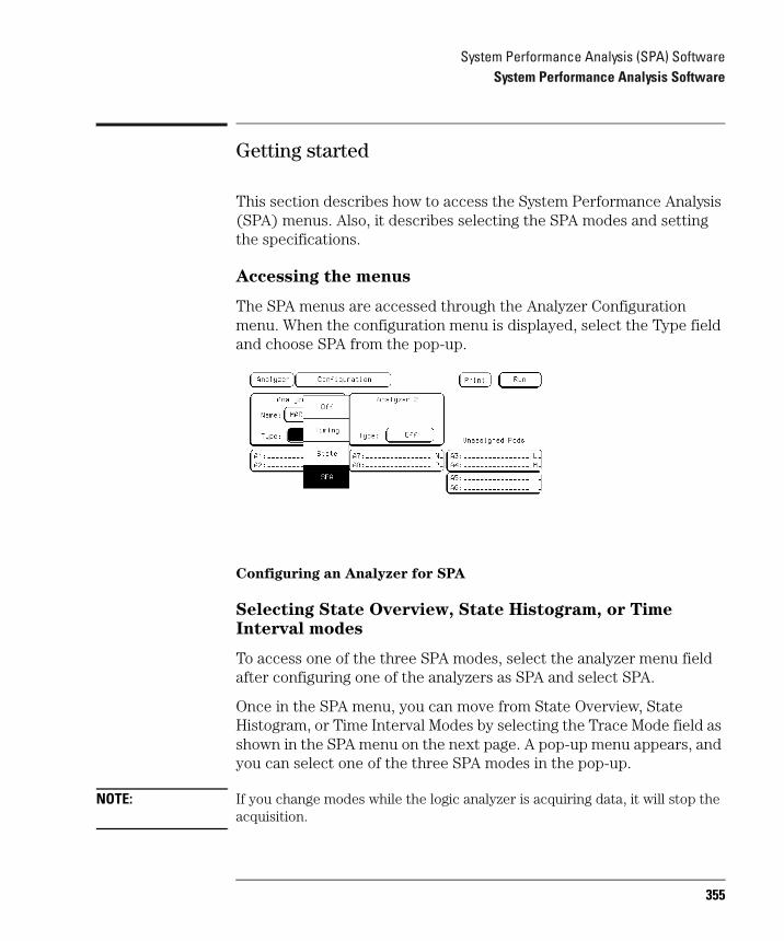
System Performance Analysis (SPA) SoftwareSystem Performance Analysis Software
Getting started
This section describes how to access the System Performance Analysis (SPA) menus. Also, it describes selecting the SPA modes and setting the specifications.
Accessing the menus
The SPA menus are accessed through the Analyzer Configuration menu. When the configuration menu is displayed, select the Type field and choose SPA from the pop-up.
Configuring an Analyzer for SPA
Selecting State Overview, State Histogram, or Time
Interval modes
To access one of the three SPA modes, select the analyzer menu field after configuring one of the analyzers as SPA and select SPA.
Once in the SPA menu, you can move from State Overview, State Histogram, or Time Interval Modes by selecting the Trace Mode field as shown in the SPA menu on the next page. A pop-up menu appears, and you can select one of the three SPA modes in the pop-up.
NOTE: If you change modes while the logic analyzer is acquiring data, it will stop the acquisition.
355
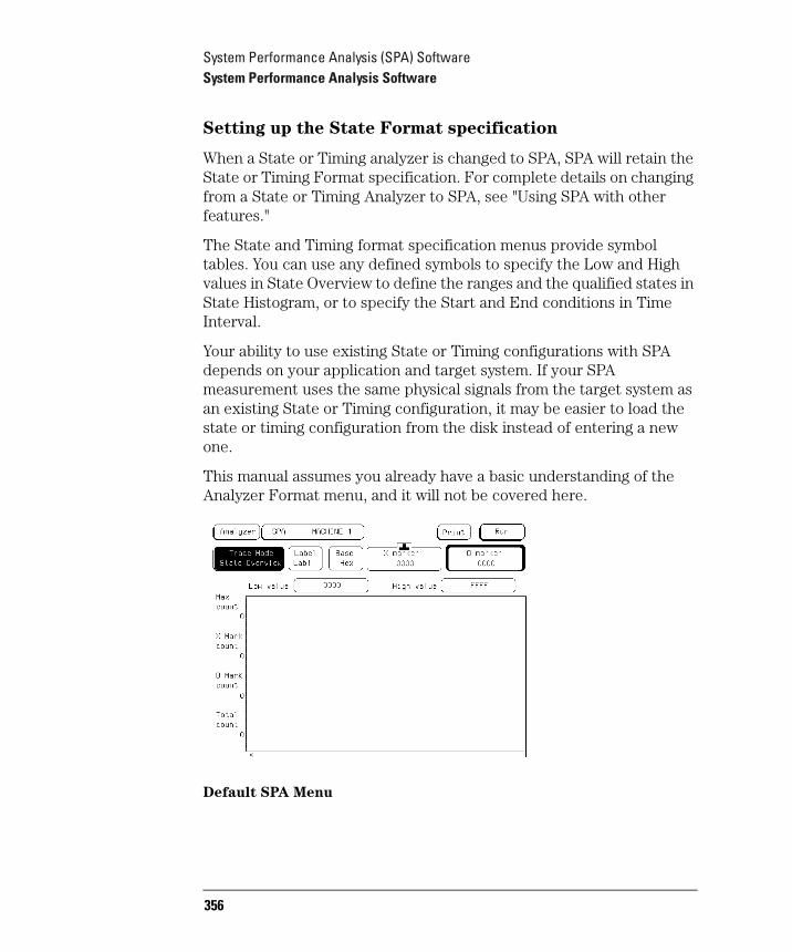
System Performance Analysis (SPA) SoftwareSystem Performance Analysis Software
Setting up the State Format specification
When a State or Timing analyzer is changed to SPA, SPA will retain the State or Timing Format specification. For complete details on changing from a State or Timing Analyzer to SPA, see "Using SPA with other features."
The State and Timing format specification menus provide symbol tables. You can use any defined symbols to specify the Low and High values in State Overview to define the ranges and the qualified states in State Histogram, or to specify the Start and End conditions in Time Interval.
Your ability to use existing State or Timing configurations with SPA depends on your application and target system. If your SPA measurement uses the same physical signals from the target system as an existing State or Timing configuration, it may be easier to load the state or timing configuration from the disk instead of entering a new one.
This manual assumes you already have a basic understanding of the Analyzer Format menu, and it will not be covered here.
Default SPA Menu
356
System Performance Analysis (SPA) SoftwareSystem Performance Analysis Software
SPA measurement processes
This section introduces you to the measurement processes of the System Performance Analysis (SPA) software. It tells you how to select the appropriate trace mode and labels. It also explains how SPA samples and sorts data.
Selecting and changing trace modes
SPA has three trace modes: State Overview, State Histogram, and Time Interval. These are selected by the Trace Mode field in the SPA data display.
Only the currently displayed trace mode is affected during an acquisition. While acquiring and viewing data in one trace mode, the other two trace modes are not updated. If the trace mode or any other critical variable is changed during an acquisition, the logic analyzer stops the acquisition and displays "Warning: Run HALTED due to variable change."
Each trace mode only performs statistics on its own database. Therefore, if acquisitions are completed in two different trace modes, the two modes will not contain the same data.
For example, you select the State Overview mode and press the Run key. After the data accumulates for a period, press Stop. You then select the Time Interval mode and the screen is blank since no data has been acquired in this mode. You again press Run, and let data accumulate and press Stop. In this example, two separate data sets are acquired, the first for State Overview mode, the second for Time Interval. You can now move between the modes and see the correct data for the associated measurement.
This separate acquisition data applies to all three trace modes. In this way, three separate views of the target system can be acquired and stored in SPA.
357
System Performance Analysis (SPA) SoftwareSystem Performance Analysis Software
Sampling methods and data sorting
SPA provides a statistical summary of target system behavior over time. The greater the number of samples, the more accurate the statistics. Therefore, SPA should always be run in the Repetitive mode. By doing this, the analyzer will continue to sample the data and update the display until Stop is pressed or until a sampling variable is changed on the display.
After SPA completes an acquisition, each sample in the current acquisition is compared to the ranges or buckets for the current trace mode. If the sample matches a range or bucket, it is sorted into that range or bucket. This process is repeated for every sample in the acquisition. After the entire acquisition has been sorted, the histograms and displayed statistics are updated, and the analyzer is re-armed for the next acquisition.
Refer to the following sections on the three trace modes for details on sorting criteria and statistical computation.
Between each successive acquisition, there is blind time during which the captured data is unloaded and sorted, the display is updated, and the analyzer is restarted. The length of the blind time is a function of the complexity of the SPA measurement.
Selecting and changing labels
A label in Agilent Technologies logic analyzers is defined in the Format menu. A label is any named group of 32 or fewer data channels.
The State Overview and State Histogram modes monitor one label at a time. Any labels that are defined in the Format Specification are available. A typical example is the ADDR (address) label used in many of the Agilent Technologies inverse assembler configurations. Often, SPA measurements will use the ADDR label to monitor memory activity.
358

System Performance Analysis (SPA) SoftwareSystem Performance Analysis Software
Qualified State Histogram and Time Interval modes use all of the labels in the Format Specification to define either the qualified state or the start and stop events, respectively. While State Overview and State Histogram deal with recorded states, Time Interval deals with time.
NOTE: Changing from one label to another in State Overview or State Histogram mode or changing the Start or End pattern in Time Interval erases any configuration and data for the original label. When returning to the original label, the display returns to its default mode. Loss of configurations and data when changing between labels can be prevented by saving configurations of interest to the disk before making the change, or by printing the results.
State Overview mode
State Overview mode is an X-versus-Y chart of the activity on a specified label. It provides a global view of the distribution of activity of the target system signals grouped under the specified label.
X axis scaling. The X axis represents the defined range of the specified label and is divided into a series of buckets, or smaller ranges. The range of the X axis is defined by the Low value and High value fields, and is divided equally among 256 buckets. For example, if the range defined by the low and high values is 1100, then 1100 divided by 256 equals 4.29. This value will be rounded up to 5, each bucket will have a range of 5, and only 220 buckets will be used (1100/5 = 220). The display grid will be truncated on the right because only 220 buckets are displayed.
If the full range of the label or the portion of the label defined by the Low value and High value is less than 255, then the number of buckets will be the difference between the Low and High values.
The Low and High values can be specified as discrete values in Binary, Octal, Decimal, or Hexadecimal. If Symbols have been defined in the Format Specification, they can also be used for the low and high values.
359

System Performance Analysis (SPA) SoftwareSystem Performance Analysis Software
Data sampling and sorting. When Run is pressed, all input channels defined in the Format Specification are sampled. Once acquired, the sampled data is sorted into the buckets of the specified label, and the State Overview display is updated. The acquisition is repeated until Stop is pressed or until a display variable is changed.
Y axis scaling. The display builds a vertical histogram where the Y axis represents the relative number of occurrences in each of the buckets. As successive acquisitions are acquired and sorted, the display is constantly re-scaled vertically so that the upper limit of the Y axis represents the largest number of occurrences in any bucket.
The Y axis maximum limit is displayed in Max count.
Total count. The Total count field is the total number of states sampled over the entire label range since the measurement was started.
X and O markers. Markers can be placed on any bucket to determine the number of occurrences in that bucket. The X Mark count and O Mark count fields display the number of occurrences at the markers. The markers move only on the bucket boundaries.
The range of each bucket can be determined by selecting the Xmarker or Omarker fields and noting the change in the marker value in the pop-up as the marker is moved slowly across the display.
360

System Performance Analysis (SPA) SoftwareSystem Performance Analysis Software
Example State Overview example
An example of a State Overview measurement is testing for access to a reserved area of memory. In this case, the address bus of the target system would need to be grouped under a single label, such as ADDR. By selecting the ADDR label in State Overview mode, and by defining the full range of the label (Low value = 0000, High value = FFFF with a 16-bit ADDR label), activity over the entire address range can be monitored. Access into reserved memory is easily identified.
By selecting only the range of the reserved area of memory with the Low and High values, the number of address values per bucket is decreased and a more detailed analysis can be performed.
The figure below shows a State Overview display.
SPA State Overview Menu
361
System Performance Analysis (SPA) SoftwareSystem Performance Analysis Software
State Histogram mode
State Histogram mode displays relative activity of ranges of a specified label. The ranges can also be compared to activity on the rest of the label not defined in the ranges. Data qualification is possible with State Histogram, so data can be filtered during acquisition.
Data sampling and sorting. When Run is pressed, all input channels defined in the Format Specification are sampled. Once acquired, each sample in the acquisition is compared to each defined range. If the sample value is inclusively within the range and if the range is on, the count for that range is incremented, then the State Histogram display is updated. The acquisition is repeated until Stop is pressed or until a display variable is changed.
The histogram is displayed on a percentage scale, and each bar represents the fraction of all samples in that range. For example, if a bar reaches the 40% value on the display, then the range for that bar contains 40% of all the samples displayed. If the total percentages of all bars equals greater than 100%, then ranges have been overlapped and data has been counted twice.
State Histogram vs. State Overview. State Histogram is similar to State Overview, but there are key differences between the two modes. State Overview shows relative distribution of activity over a single contiguous range of a label. State Histogram also allows several non-contiguous ranges of a label to be defined.
State Overview requires minimal setup, and provides a quick overview of system activity. State Histogram requires more setup, but provides greater resolution and measurement flexibility.
362
System Performance Analysis (SPA) SoftwareSystem Performance Analysis Software
State Overview mode does not display data that falls out of the range of its Low and High values. State Histogram, on the other hand, has an "Other States included/excluded" feature that will present a histogram of any activity that does not fall into the defined ranges (see "Other States included/ excluded," later in this section).
State Overview samples and displays all activity on the specified label. But State Histogram allows data qualification so that only activity of interest is sampled and displayed (see "Trace Type: All States vs. Qualified States," later in this section).
Range specifiers. A maximum of 11 ranges are available. The ranges are defined by specifying a low and high value on the specified label and by a name you define. The ranges need not be contiguous. If two ranges overlap in any manner, acquired data will be counted in both ranges.
If a range has a low and high value and a name defined, and the range is turned off, it will retain the low and high value and name when turned back on.
User-defined ranges vs. symbols. When defining low and high values for the State Histogram ranges, you may use symbols instead of entering discrete values. Symbols can only be used for labels selected in the State Histogram mode if they are defined in the Format Specification, and only if the base in the State Histogram menu is set to Symbol.
Pattern or range symbols defined in the Format Specification can be used to set the low or high value of a range.
Total samples. The Total samples field displays the total number of samples in all the displayed ranges. If Other States included is selected, then total samples is the total of all displayed samples plus the other states. If any ranges are overlapped and samples fall in multiple buckets, these samples are only counted once in total samples.
363
System Performance Analysis (SPA) SoftwareSystem Performance Analysis Software
Number of samples per range. Displayed next to each bar is a value representing the number of samples for that range. The ratio of these values to total samples determines the relative size of the histograms. These values are updated as the repeated acquisitions are sorted and displayed.
Other States included/excluded. Usually the defined ranges will not cover the entire range of the specified label. The Other States included/ excluded field provides an optional histogram showing all activity on the specified label that does not fall within any of the defined ranges. By selecting excluded, the relative activity of only the defined ranges is displayed. If included is selected, the "other" histogram appears under the ranges.
If a range is turned off, any activity in that range is included in Other States. The activity of a turned off range is included in the other range whether included or excluded other states is displayed or not.
Trace Type: All States vs. Qualified States. State Histogram mode can qualify data as it is sampled. Qualifying data while sampling allows only data of interest to be stored, while the rest is thrown away.
When Trace Type is set to Qualified States, a new field appears in the upper row of the display. The new field, Specify States, is where the data qualification is defined. The data qualification is not limited only to the label selected in the State Histogram menu. It is defined over all labels in the Format Specification as a combination of values, in the current base, and don't cares.
For example, a microprocessor target system memory may contain two arrays. In State Histogram, the address ranges of the arrays can be defined and the relative activity in the arrays monitored. But, what if you only want to monitor writes to the array? In this case, you can define the data qualification as "Memory Write" on the STATUS label.
States that do not meet the qualification criteria are not stored by the analyzer, so they are not included in Other States.
364
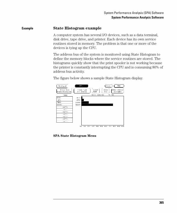
System Performance Analysis (SPA) SoftwareSystem Performance Analysis Software
Example State Histogram example
A computer system has several I/O devices, such as a data terminal, disk drive, tape drive, and printer. Each device has its own service routines stored in memory. The problem is that one or more of the devices is tying up the CPU.
The address bus of the system is monitored using State Histogram to define the memory blocks where the service routines are stored. The histograms quickly show that the print spooler is not working because the printer is constantly interrupting the CPU and is consuming 80% of address bus activity.
The figure below shows a sample State Histogram display.
SPA State Histogram Menu
365

System Performance Analysis (SPA) SoftwareSystem Performance Analysis Software
Time Interval mode
Time Interval mode shows distribution of the execution time of a single event. The event is defined by specifying Start and End conditions as patterns across all labels defined in the Format Specification.
Data sampling and sorting. When you press Run, the analyzer samples the target system using the definitions entered in the Format Specification. During acquisition, the state analyzer searches the data for the start and end conditions, and uses the analyzer's time tag feature to time the event. The time durations for each Start/End pair are then sorted into user-definable time interval ranges on the display. The acquisition is repeated until Stop is pressed or until a display variable is changed.
Because time tags are not available in the half-channel mode as specified in the Format menu, time interval mode will not function when half-channel mode is selected.
After the data is sampled, timed, and sorted, the histogram for each time interval range is updated.
If two time intervals are adjacent and have a common boundary (the upper limit of one equals the lower limit of the next), and a sampled time interval falls on the common boundary, the sample will be sorted into the higher time interval.
Start/End conditions. Start and end conditions for Time Interval are specified on all labels defined in the Format Specification as a combination of values, in the current base, and don't cares.
If a start or end condition is not found during an acquisition, the histogram will not change. The analyzer will only update when a start and stop event are both found.
366
System Performance Analysis (SPA) SoftwareSystem Performance Analysis Software
Start and end conditions need not be adjacent in the data stream. For example, when the state analyzer sees the specified start condition, it starts the timer. If the start condition occurs again before the end condition occurs, the timer will not be reset.
For measurement purposes, the analyzer measures the time between the first occurrence of the start condition and the first occurrence of the stop condition.
Time Interval ranges. A maximum of 8 time interval ranges are available. Each range has a lower and upper limit which can be entered manually. The Auto-range feature will automatically scale the eight ranges. The minimum allowable limit is 0ns, the maximum 9,999,999 seconds.
Ranges do not have to be contiguous. However, gaps between ranges increase the risk of missed data. If two ranges overlap, data will be counted in both ranges. This applies to any number of overlapping ranges, or any portions of overlapping ranges. Common boundaries of adjacent ranges are not considered to be overlapped.
A range can be turned off by setting the lower and upper values to zero.
Auto-range. The Time Interval ranges can be scaled quickly by selecting "Auto-range." This option requires a global Minimum time and Maximum time for the eight time interval ranges. The eight ranges are then scaled using either a log scale or linear scale.
All the ranges may be quickly initialized to off by selecting Auto-range, setting Minimum time and Maximum time to zero, and performing a linear scale.
The smallest increment allowable using Auto-scale is 10 ns. If the time interval defined by the minimum and maximum times is too small to scale8 ranges, Auto-range will scale as many as possible and exclude some upper time interval ranges. The maximum resolution of each time interval is 10 ns.
367
System Performance Analysis (SPA) SoftwareSystem Performance Analysis Software
Min, Max, and Avg Time Statistics. The Time Interval mode display shows three statistics: Maximum (Max) time, Minimum (Min) time, and Average (Avg) time. These values are displayed whether or not they fall into any of the time interval ranges. Therefore, they are helpful in determining if the appropriate time intervals have been chosen.
The maximum resolution of the statistics is 8 ns.
Total samples. Total samples is displayed above the histogram. A sample is defined as one Start/End pair. The Total samples field is not updated until the analyzer's memory is full or until Stop is pressed.
368
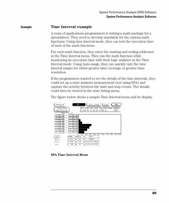
System Performance Analysis (SPA) SoftwareSystem Performance Analysis Software
Example Time Interval example
A team of applications programmers is writing a math package for a spreadsheet. They need to develop standards for the various math functions. Using time interval mode, they can test the execution time of each of the math functions.
For each math function, they enter the starting and ending addresses in the Time Interval menu. They run the math function while monitoring its execution time with their logic analyzer in the Time Interval mode. Using Auto-range, they can quickly vary the time interval ranges for either greater time coverage or greater time resolution.
If the programmers wanted to see the details of the time intervals, they could set up a state analyzer measurement (not using SPA) and capture the activity between the start and stop events. The details could then be viewed in the state listing menu.
The figure below shows a sample Time Interval menu and its display.
SPA Time Interval Menu
369
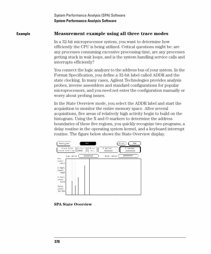
System Performance Analysis (SPA) SoftwareSystem Performance Analysis Software
Example Measurement example using all three trace modes
In a 32-bit microprocessor system, you want to determine how efficiently the CPU is being utilized. Critical questions might be: are any processes consuming excessive processing time, are any processes getting stuck in wait loops, and is the system handling service calls and interrupts efficiently?
You connect the logic analyzer to the address bus of your system. In the Format Specification, you define a 32-bit label called ADDR and the state clocking. In many cases, Agilent Technologies provides analysis probes, inverse assemblers and standard configurations for popular microprocessors, and you need not enter the configuration manually or worry about probing issues.
In the State Overview mode, you select the ADDR label and start the acquisition to monitor the entire memory space. After several acquisitions, five areas of relatively high activity begin to build on the histogram. Using the X and O markers to determine the address boundaries of these five regions, you quickly recognize two programs, a delay routine in the operating system kernel, and a keyboard interrupt routine. The figure below shows the State Overview display.
SPA State Overview
370
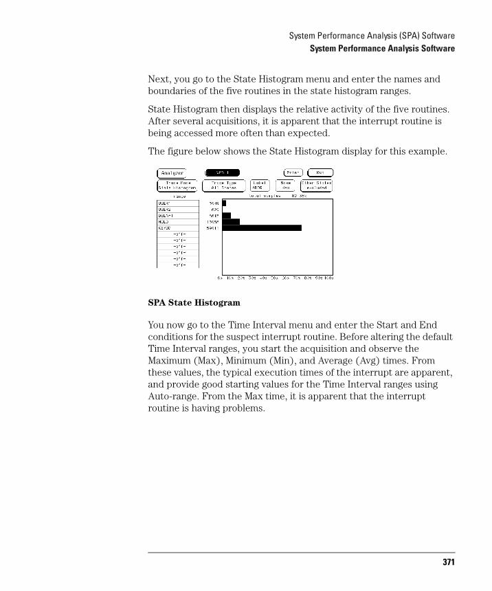
System Performance Analysis (SPA) SoftwareSystem Performance Analysis Software
Next, you go to the State Histogram menu and enter the names and boundaries of the five routines in the state histogram ranges.
State Histogram then displays the relative activity of the five routines. After several acquisitions, it is apparent that the interrupt routine is being accessed more often than expected.
The figure below shows the State Histogram display for this example.
SPA State Histogram
You now go to the Time Interval menu and enter the Start and End conditions for the suspect interrupt routine. Before altering the default Time Interval ranges, you start the acquisition and observe the Maximum (Max), Minimum (Min), and Average (Avg) times. From these values, the typical execution times of the interrupt are apparent, and provide good starting values for the Time Interval ranges using Auto-range. From the Max time, it is apparent that the interrupt routine is having problems.
371
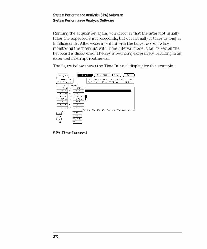
System Performance Analysis (SPA) SoftwareSystem Performance Analysis Software
Running the acquisition again, you discover that the interrupt usually takes the expected 8 microseconds, but occasionally it takes as long as 8milliseconds. After experimenting with the target system while monitoring the interrupt with Time Interval mode, a faulty key on the keyboard is discovered. The key is bouncing excessively, resulting in an extended interrupt routine call.
The figure below shows the Time Interval display for this example.
SPA Time Interval
372
System Performance Analysis (SPA) SoftwareSystem Performance Analysis Software
Using State Overview, State Histogram, and Time Interval
This section explains how to select the display fields, set up the logic analyzer and use the State Overview, State Histogram and Time Interval modes of SPA.
Setting up the logic analyzer
This section assumes you have defined the Format and have connected the logic analyzer probes to the target system. For complete details on these topics, refer to the appropriate reference section for your analyzer.
For a detailed description of State Overview, State Histogram, and Time Interval mode measurement processes, refer to the previous section, "SPA measurement processes."
Using State Overview mode
Choosing a label to monitor. To specify a label to monitor, select the "Label" field in the State Overview menu. The pop-up shows a list of all the labels defined in the Format Specification. From this list, choose the label you want to monitor.
NOTE: Changing from one label to another will erase the display setup for the first label. If you want to change to a different label, but don't want to lose the setup for the current one, first save the current one to disk or print it.
373
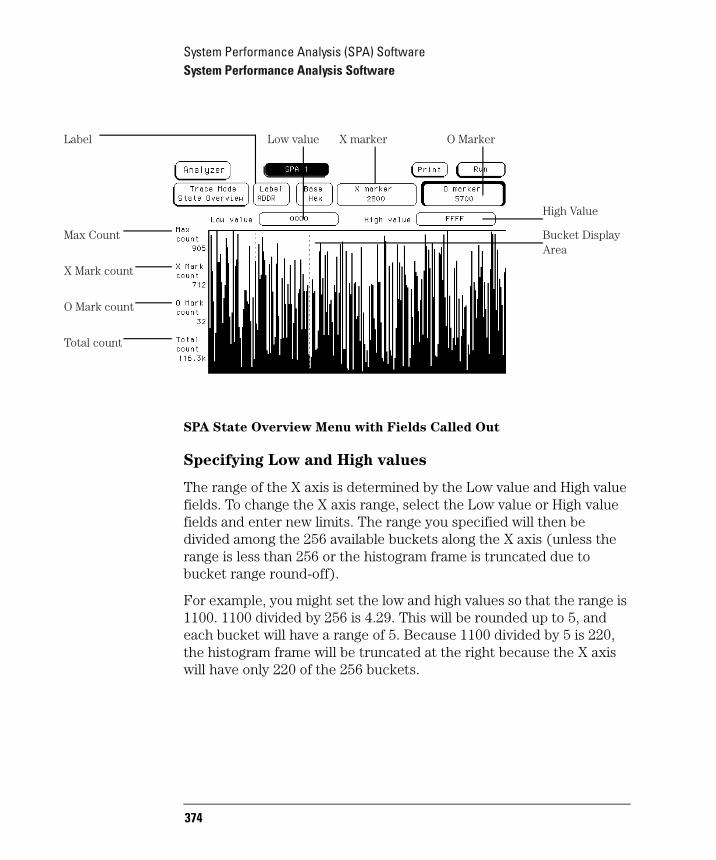
System Performance Analysis (SPA) SoftwareSystem Performance Analysis Software
SPA State Overview Menu with Fields Called Out
Specifying Low and High values
The range of the X axis is determined by the Low value and High value fields. To change the X axis range, select the Low value or High value fields and enter new limits. The range you specified will then be divided among the 256 available buckets along the X axis (unless the range is less than 256 or the histogram frame is truncated due to bucket range round-off).
For example, you might set the low and high values so that the range is 1100. 1100 divided by 256 is 4.29. This will be rounded up to 5, and each bucket will have a range of 5. Because 1100 divided by 5 is 220, the histogram frame will be truncated at the right because the X axis will have only 220 of the 256 buckets.
Label
Max Count
X Mark count
Total count
Low value X marker O Marker
High Value
Bucket Display Area
O Mark count
374
System Performance Analysis (SPA) SoftwareSystem Performance Analysis Software
The default high and low values represent the full range of the label you chose. Before changing these values, you may want to run the acquisition and acquire some data to view activity over the entire range of the label. You can then zoom in on areas of interest.
You can enter low and high values in binary, octal, decimal, hexadecimal, ASCII, or symbol.
Interpreting the histogram display
Press the blue shift key and Run to start the State Overview acquisition. As the data is sampled and sorted, the buckets along the X axis will accumulate. The relative size of the vertical bars show the distribution of activity on the label you chose. The analyzer will continue to sample, sort the data, and update the display until you press Stop or until you change a display variable.
Max count represents the current upper limit of the Y axis for the bucket with the greatest number of data samples. Max count for the limit of the Y axis will increase as the buckets fill with samples.
Read Total count to find the total number of samples taken over the specified range of the label. This is not affected by the low and high values.
Using the markers. To find the number of data samples in any bucket, select the Xmarker or Omarker field. Turn the knob to move the marker to the area of interest. Read the X Mark count or O Mark count values to determine the number of samples in the current bucket.
As you move either marker across the display, the value in the XMarker or OMarker pop-up will change. The amount of change of the marker's value represents the size of the bucket.
375

System Performance Analysis (SPA) SoftwareSystem Performance Analysis Software
Zooming in on an area of interest. When viewing the State Overview display, you may see areas of high activity and areas of little or no activity. To zoom in on one of these areas for more resolution, put the X and O markers on the boundaries of the area, then adjust the low and high values to match the X and O marker positions.
Using State Histogram mode
Choosing a label to monitor. To specify a label to monitor, select the Label field in the State Histogram display. In the pop-up, you will see a list of all the labels defined in the Format specification. From this list, choose the label you want to monitor.
NOTE: Changing from one label to another will erase the display setup for the first label. If you want to change to a different label, but do not want to lose the setup for the current one, save the current one to a disk.
Defining the ranges. To define a range on the specified label, select one of the 11 range fields. When you select one of the 11 ranges, you will see the Range Definition pop-up. This pop-up has fields where you enter the low and high value, a name for the range, and whether the range is on or off.
SPA State Histogram Menu
376
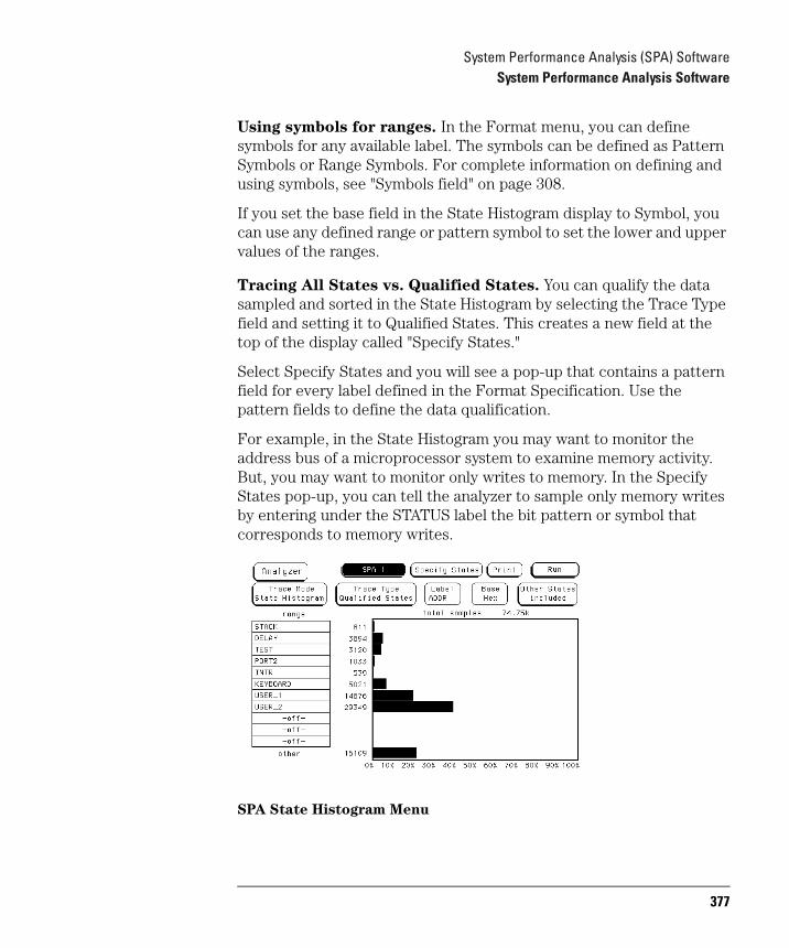
System Performance Analysis (SPA) SoftwareSystem Performance Analysis Software
Using symbols for ranges. In the Format menu, you can define symbols for any available label. The symbols can be defined as Pattern Symbols or Range Symbols. For complete information on defining and using symbols, see "Symbols field" on page 308.
If you set the base field in the State Histogram display to Symbol, you can use any defined range or pattern symbol to set the lower and upper values of the ranges.
Tracing All States vs. Qualified States. You can qualify the data sampled and sorted in the State Histogram by selecting the Trace Type field and setting it to Qualified States. This creates a new field at the top of the display called "Specify States."
Select Specify States and you will see a pop-up that contains a pattern field for every label defined in the Format Specification. Use the pattern fields to define the data qualification.
For example, in the State Histogram you may want to monitor the address bus of a microprocessor system to examine memory activity. But, you may want to monitor only writes to memory. In the Specify States pop-up, you can tell the analyzer to sample only memory writes by entering under the STATUS label the bit pattern or symbol that corresponds to memory writes.
SPA State Histogram Menu
377
System Performance Analysis (SPA) SoftwareSystem Performance Analysis Software
Interpreting the histogram display. Press the blue shift key and Run to start the State Histogram acquisition. The relative activity over the ranges you defined is displayed as histograms (see the figure on the previous page). The total samples field shows the total number of data samples displayed in all of the ranges. The number of samples for each range is displayed to the left of each histogram.
The percentage amounts of the histograms total 100% (note the scale at the bottom of the display). If they add up to more than 100%, you have overlapped two or more ranges, and the data samples are being counted in multiple ranges.
The analyzer will continue to sample, sort the data, and update the display until you press Stop or change a display variable.
Other States included/excluded. The histograms show the relative distribution of activity over the ranges you have defined. In most cases, the ranges will not cover the full range of the label you chose to monitor.
To view the activity over the entire range of the label, including activity not covered by the ranges, select the Other States field and change it to included. Another histogram bar called "other" will appear at the bottom of the display. This will show activity not covered by the ranges. You can toggle included/excluded if the analyzer is stopped or if it is running because it only affects the display and not the accumulated data that has been acquired.
Note that changing between included and excluded changes the absolute sizes of the histograms. Unless you have defined overlapping ranges, the total percentage size of the all the range histograms plus the histogram for other should equal 100%.
378
System Performance Analysis (SPA) SoftwareSystem Performance Analysis Software
Using Time Interval mode
Use Time Interval mode to determine the distribution of time between two specific events. The state analyzer uses the time tag feature to time the event; thus, in Time Interval mode, the minimum state clock period is 10 ns.
Specifying an event
To use Time Interval mode, you must define an event that you want timed. At the bottom of the display, note the Start and End fields. To define an event, select the appropriate labels in the Start and End fields to define the boundaries.
For example, start and end might be the beginning and ending addresses of a subroutine stored in memory. If you are timing a counter period, start and end might be the initial and final count values.
Note that in start and end, you are not limited to a single label. You define the event over all available labels as patterns including don't cares. Be sure that the start and end conditions actually occur in the target system or the analyzer will not find the timing reference points and will not make the time interval measurement. You may want to use the state analyzer (not SPA) to verify that the Start and Stop events actually occur.
379
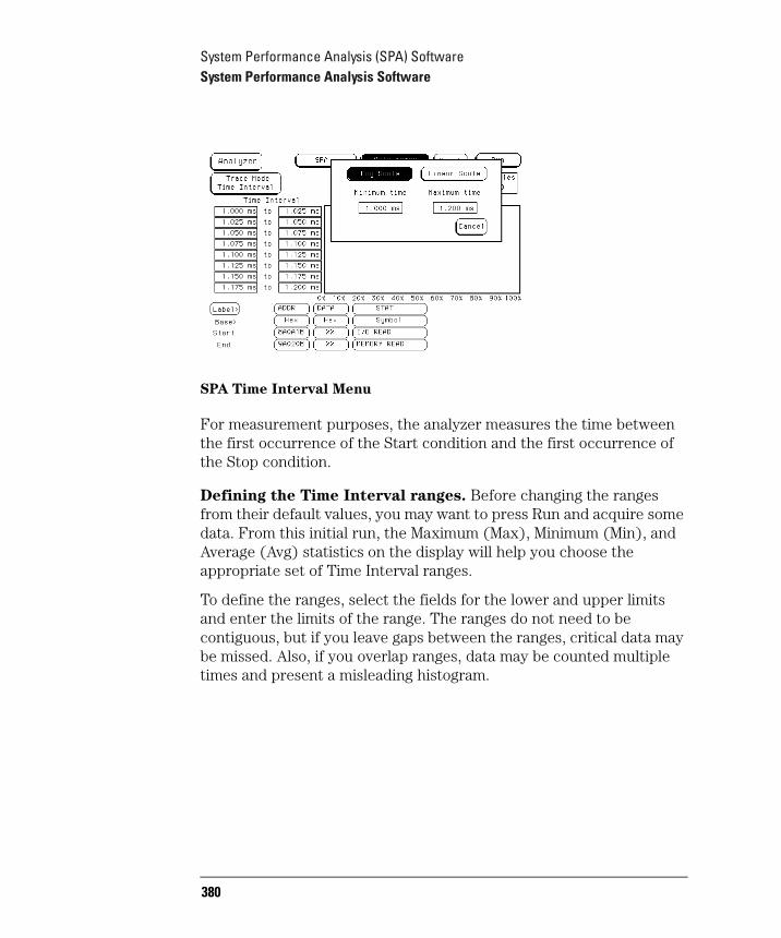
System Performance Analysis (SPA) SoftwareSystem Performance Analysis Software
SPA Time Interval Menu
For measurement purposes, the analyzer measures the time between the first occurrence of the Start condition and the first occurrence of the Stop condition.
Defining the Time Interval ranges. Before changing the ranges from their default values, you may want to press Run and acquire some data. From this initial run, the Maximum (Max), Minimum (Min), and Average (Avg) statistics on the display will help you choose the appropriate set of Time Interval ranges.
To define the ranges, select the fields for the lower and upper limits and enter the limits of the range. The ranges do not need to be contiguous, but if you leave gaps between the ranges, critical data may be missed. Also, if you overlap ranges, data may be counted multiple times and present a misleading histogram.
380
System Performance Analysis (SPA) SoftwareSystem Performance Analysis Software
Using Auto-range. To quickly set up all 8 time interval ranges, select the Auto-range field. Enter the minimum time and maximum time for all 8 ranges combined. Then, when you select Log Scale or Linear Scale, all 8 ranges will be scaled accordingly between the Minimum and Maximum times. See the figure on the previous page for the Auto-range pop-up. Common boundaries of adjacent ranges are not considered overlapped. Values that fall on the common boundary will be included in the highest range.
A fast way to set up the Time Interval display is to define your Start and End events and select Run using the default ranges. Select Repetitive Run mode. After accumulating data for a while, press Stop. Then select Auto-range and enter the Min time and Max time display statistics in the Auto-range Minimum time and Maximum time fields. When you select Log Scale or Linear Scale, the ranges will be defined automatically.
Interpreting the histogram display. As the analyzer samples the data, it searches for Start/End event pairs. One event pair is considered one sample. The time value for each event pair is compared to each defined time interval range. The range's count is incremented if the time value falls within that range.
381
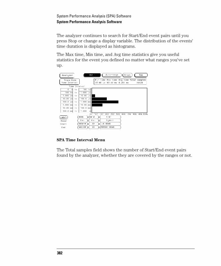
System Performance Analysis (SPA) SoftwareSystem Performance Analysis Software
The analyzer continues to search for Start/End event pairs until you press Stop or change a display variable. The distribution of the events' time duration is displayed as histograms.
The Max time, Min time, and Avg time statistics give you useful statistics for the event you defined no matter what ranges you've set up.
SPA Time Interval Menu
The Total samples field shows the number of Start/End event pairs found by the analyzer, whether they are covered by the ranges or not.
382
System Performance Analysis (SPA) SoftwareSystem Performance Analysis Software
Using SPA with other features
Programming with SPA
SPA is programmable. Refer to the Agilent Technologies 1670G Series Logic Analyzers Programmer's Guide for SPA commands. The Programmer's Guide is available as an option with the logic analyzer. Contact your Agilent Technologies Sales Office for more information.
Changing between SPA and a State/Timing Analyzer
If you have configured a state or timing analyzer in the logic analyzer, you can quickly change to SPA, or from SPA to a state or timing analyzer. You can use the same Format Specification in your SPA measurements as you did in your state or timing analysis measurements.
To change between a state analyzer and SPA, go to the Analyzer Configuration menu, select the Type field, and select SPA from the list.
When SPA is selected, a separate trace specification definition is used. Even though the Qualified State Histogram and Time Interval modes use the same pattern recognizers as SPA, the SPA definitions are kept separate from those entered in the state or timing analyzer mode. As a result, switching between SPA and state or timing recovers the user's original pattern recognizers for the selected mode.
Any Symbols in the Format Specification will also carry over to SPA.
383
System Performance Analysis (SPA) SoftwareSystem Performance Analysis Software
Using SPA in Group Runs
The 1670G-series logic analyzers allow you to set up group runs using the Arming Control field of the other machine's Trigger menu.
By its statistical nature, SPA runs best as a repetitive measurement system. Therefore, if you include SPA in a Group Run, it will execute and update the SPA displays, but the data may not be acquired in a statistically random-repetitive fashion. It may not represent a true statistical analysis of your target system.
Another way to make SPA measurements in conjunction with other analysis is to run SPA independently (do not include it in the Group Run), and set up the other machines as you normally would. In this way, SPA will provide a truer statistical analysis of your target system.
384

11
Logic Analyzer Concepts
385
Logic Analyzer ConceptsLogic Analyzer Concepts
Logic Analyzer ConceptsUnderstanding how the analyzer does its job will help you use it more effectively and minimize measurement problems. This chapter explains the structure of the file system, the details of transitional timing mode, the general operation of the trigger sequence, and the details of the hardware.
386
Logic Analyzer ConceptsThe File System
The File SystemThe 1670G-series logic analyzers have a complex internal file system. Many of the file attributes are only accessible over a LAN connection. From the logic analyzer's front panel, the only parts of the file system you can examine are the hard disk drive and the flexible disk drive. The hard disk drive contains the /SYSTEM directory with the X Window fonts and some example files, and also whatever other files and directories you have created on it. The flexible disk drive directory contains whatever files are on the disk in the disk drive.
See Also The LAN section of this book on page 478 for more information on the LAN-accessible portions of the file system.
387

Logic Analyzer ConceptsThe File System
Directories
Hard disk drive
When you receive the logic analyzer, the hard disk drive is already DOS-formatted. The factory also creates a directory on the hard disk drive named "/SYSTEM". The /SYSTEM directory is intended to store system software such as backup copies of the operating system files and the performance verification files. When you receive your logic analyzer, the /SYSTEM directory already contains two X Window font files and several files containing examples.
The files on the hard disk drive are not essential to the logic analyzer's correct operation. However, you can store important files such as optional software, autoload files, configurations, and software backups here. You can configure the logic analyzer to Autoload files from the hard disk at power-up.
When the logic analyzer searches for autoload files and software options, it first looks in the flexible disk drive. If the flexible disk drive contains an autoload file and two software options, the analyzer does not check the hard disk drive. If some of these were not found, the analyzer next checks the hard drive's /SYSTEM directory.
You can manually copy files, such as performance verification files, to the /SYSTEM directory, but they will not necessarily be installed when the analyzer powers up. To automatically load software, follow the installation instructions provided with the software. It will change the power-up sequence to include the software option and also copy the files to the /SYSTEM directory.
Flexible disk drive
The flexible disk drive reads 3.5-inch flexible disks in both DOS and LIF format. If a disk is in the drive when the analyzer is turned on, the analyzer checks the disk for software and autoload files. If these files are found, they are loaded into the analyzer.
388
Logic Analyzer ConceptsThe File System
File types
Standard file types
The file type is shown in a small display box centered on the line above the file listings.
autoload_file. indicates the file, almost always named AUTOLOAD, is an autoload file. The file description indicates if the autoload file is enabled or disabled, and the file it autoloads. Autoload files are created by executing "Autoload" in the System Disk menu.
167xan_config. indicates the file is a 1670G-series logic analyzer configuration. These files are created by executing "Store Analyzer" or "Store All" in the System Disk menu.
167x_cnfg. indicates the file is a system configuration. These files are created by executing "Store System" or "Store All" in the System Disk menu.
DOS. indicates the file is in DOS format. It might be a screenshot or a file created on a PC and copied to the disk. These files are not loadable.
directory. indicates the file is a directory and that you can change to that directory. Other files are within it.
16[6/7]x_opt. indicates the file is software that can be used with either the Agilent Technologies 1660 or 1670 family of logic analyzers.
389
Logic Analyzer ConceptsThe File System
167xsc_config. indicates the file is an oscilloscope configuration. These files are created by executing "Store Scope" or "Store All" in the System Disk menu.
16522_cnfg. indicates that the file is a pattern generator configuration. These files are created by executing "Store Patt Gen" in the System Disk menu.
Filename endings
Filename endings are not restricted to certain types. These descriptions are just general guidelines. In addition, other tools you use with the logic analyzer will likely have their own set of filename endings.
[none]. Of the common file types you can create using the logic analyzer, only the ASCII listings do not have a default ending. If you supply one in the Print to Disk filename field, that ending will be used, but no ending is automatically appended as with other filenames.
Three other types of files commonly do not have a default ending: directories, software, and autoload files. Check the file type field to be sure what type of file you are selecting.
._A. This ending is appended to analyzer configuration files created with the Store operation from the System Disk menu.
._B. This ending is appended to oscilloscope and pattern generator configuration files created with the Store operation from the System Disk menu.
.__ . This ending is appended to system configuration files created with the Store operation from the System Disk menu.
.TIF. This ending is appended to TIFF version 5.0-format screenshots created with the Print to Disk function.
.EPS. This ending is appended to EPS-format screenshots created with the Print to Disk function.
.PCX. This ending is appended to PCX-format screenshots created with the Print to Disk function.
390

Logic Analyzer ConceptsThe Trigger Sequence
The Trigger Sequence1670G-series logic analyzers have triggering and data storage features that allow you to capture only the system activity of interest. Understanding how these features work will help you set up analyzer trigger specifications that satisfy your measurement needs.
In both the state and timing analyzers, the trigger sequence acts as a filtering mechanism, with a minimum of two steps and a maximum of twelve steps in the state analyzer and ten steps in the timing analyzer. Some trigger functions may use more than one step. The steps are the sequence level specifications. The analyzer searches for a trigger sequence by matching input values on the pods to branch conditions, which control transitions between sequence levels. You can insert or delete levels to make the trigger sequence as simple or complex as is needed for your application.
391
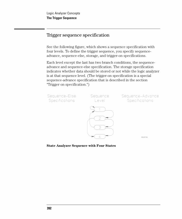
Logic Analyzer ConceptsThe Trigger Sequence
Trigger sequence specification
See the following figure, which shows a sequence specification with four levels. To define the trigger sequence, you specify sequence-advance, sequence-else, storage, and trigger-on specifications.
Each level except the last has two branch conditions, the sequence-advance and sequence-else specification. The storage specification indicates whether data should be stored or not while the logic analyzer is at that sequence level. (The trigger-on specification is a special sequence-advance specification that is described in the section "Trigger on specification.")
State Analyzer Sequence with Four States
392
Logic Analyzer ConceptsThe Trigger Sequence
Sequence-advance specification
The sequence-advance branch, sometimes called the "if" branch or primary branch, always branches to the next level. You can specify the following kinds of sequence-advance specifications:
Find (or Then find) "<TERM>" <OCCURS> time(S)
Find (or Then find) "<TERM>" <TIME PERIOD>
If the <TERM> is found <OCCURS> number of times or the <TERM> remains stable for <TIME PERIOD>, the analyzer advances to the next sequence level.
Sequence-else specification. The sequence-else branch, sometimes called the "else if" branch or secondary branch, may branch to any other state, including the current state, a previous state, or a later state. The sequence-else specification looks like the following:
Else on "<TERM>" go to level <sequence level>
If the Sequence-Else specification is satisfied before the sequence-advance specification, the sequencer goes to <sequence level>.
The last state may only have a sequence-else branch specification, which may branch to the same state or a prior state.
Storage specification. In each state, a storage specification determines the data stored by the analyzer while it is searching for the sequence-advance, sequence-else, and trigger specifications. Storage specifications are defined using the same pattern, range, and timer resources available for defining branching specifications.
While storing "anystate", "no state", or "<TERM>"
Note that if you specify "no state," the analyzer still stores sequence-advance terms and TRIGGER terms unless you also set Branches Taken Not Stored in Acquisition Control in the Analyzer Trigger menu.
393
Logic Analyzer ConceptsThe Trigger Sequence
Trigger on specification. If there are branch and storage specifications for each sequence level, what does the trigger term mean? The trigger term is a special sequence-advance specification in that, when found, it locks the contents of analyzer acquisition memory. The trigger can be positioned at the beginning, middle, or end of acquisition memory.
The trigger specification can look like the following:
TRIGGER on "<TERM>" <OCCURS> times
TRIGGER on "<TERM>" <TIME PERIOD>
If the trigger term is found <OCCURS> times, or if the trigger term remains stable for <TIME PERIOD>, the trigger is captured in memory. Then the analyzer advances to the next sequence level. If you want to capture activity after the trigger is captured, define an additional sequence level and specify the desired storage qualification for post-trigger activity (for example, store anystate).
394
Logic Analyzer ConceptsThe Trigger Sequence
Analyzer resources
The sequence-advance, sequence-else, storage, and trigger-on specifications are set by a combination of a maximum of 10 pattern terms, 2 range terms, 2 timers, and 2 edge terms (for the timing analyzer only). A resource can only be assigned to one analyzer at a time.
10 pattern terms. The pattern terms, a through j, represent single states to be found on labeled sets of bits. For example, you could have an address on the address bits or a status on the status bits, or both the address and status occurring together. Pattern terms AND conditions occurring on separate labels.
2 timers. You can start, stop, continue, or pause the timers upon entry to a sequence state, then use a comparison of current timer value against a preset value to determine whether to branch to another state.
2 range terms. The range terms, Range1 and Range2, represent ranges of values to be found on labeled sets of bits. For example, you could have a range of addresses to be found on the address bus or a range of data values to be found on the data bus. Range terms are satisfied by any value within the range for "In_Range," and any value outside the range for "Out_Range."
2 edge terms (timing analyzer only). The edge terms, Edge1 and Edge2, represent edges. The edge terms can be set to catch glitches even when the timing analyzer is not in glitch mode. When an edge term comprises more than one channel, it ORs the channel conditions together and any of the specified transitions satisfy the term.
395
Logic Analyzer ConceptsThe Trigger Sequence
You can combine the pattern terms and range terms with logical operators to form complex pattern expressions in the sequence-advance, sequence-else, and TRIGGER on specifications.
For example,
Find "(<TERM1> • <TERM2>) + (<TERM3> • <TERM4>)"
Where <TERM> can be a single value on a set of labels, any value within a range of values on a set of labels, or a glitch or edge transition on a bit or set of bits.
Limitations affecting use of analyzer resources. There are limitations on the way resources can be combined to form complex pattern expressions. Resources are combined in a four-level hierarchy. First, resources are divided into two groups. The groups can be combined with AND or OR. Second, within these groups, resources are combined into pairs. Pairs can also be logically combined using AND or OR. Third, individual resources are combined into pairs using AND, NAND, OR, NOR, XOR, and NXOR. Fourth, individual resources may be included or excluded from participating in a pattern expression. You can also include the logical negation of the resource. Fifth, the timing terms are not available in the first sequence level.
The following table shows how resources are divided in the logic analyzer. Remember that some resources may not be available, depending on the analyzer configuration. For example, if you are using the analyzer as a state analyzer, the Edge1 and Edge2 resources are not available, and only one analyzer may use a resource at a time.
396
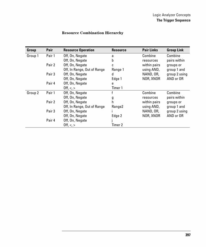
Logic Analyzer ConceptsThe Trigger Sequence
Resource Combination Hierarchy
Group Pair Resource Operation Resource Pair Links Group LinkGroup 1 Pair 1
Pair 2
Pair 3
Pair 4
Off, On, NegateOff, On, NegateOff, On, NegateOff, In Range, Out of RangeOff, On, NegateOff, On, NegateOff, On, NegateOff, <, >
abcRange 1dEdge 1eTimer 1
Combine resources within pairs using AND, NAND, OR, NOR, XNOR
Combine pairs within groups or group 1 and group 2 using AND or OR
Group 2 Pair 1
Pair 2
Pair 3
Pair 4
Off, On, NegateOff, On, NegateOff, On, NegateOff, In Range, Out of RangeOff, On, NegateOff, On, NegateOff, On, NegateOff, <, >
fghRange2iEdge 2jTimer 2
Combine resources within pairs using AND, NAND, OR, NOR, XNOR
Combine pairs within groups or group 1 and group 2 using AND or OR
397

Logic Analyzer ConceptsThe Trigger Sequence
For example, the following combinations are valid combinations for the analyzer:
(a+b) • (In_Range2 + Timer2 > 400 ns)
(c • Out_Range1) + (f xor g)
The following combinations are not valid, because resources cross pair boundaries:
a xor c
(d + Timer1 < 400 ns) • Edge1
398
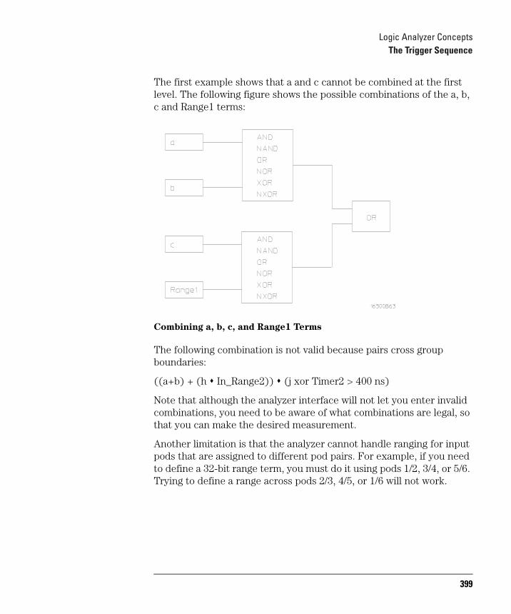
Logic Analyzer ConceptsThe Trigger Sequence
The first example shows that a and c cannot be combined at the first level. The following figure shows the possible combinations of the a, b, c and Range1 terms:
Combining a, b, c, and Range1 Terms
The following combination is not valid because pairs cross group boundaries:
((a+b) + (h In_Range2)) (j xor Timer2 > 400 ns)
Note that although the analyzer interface will not let you enter invalid combinations, you need to be aware of what combinations are legal, so that you can make the desired measurement.
Another limitation is that the analyzer cannot handle ranging for input pods that are assigned to different pod pairs. For example, if you need to define a 32-bit range term, you must do it using pods 1/2, 3/4, or 5/6. Trying to define a range across pods 2/3, 4/5, or 1/6 will not work.
399
Logic Analyzer ConceptsThe Trigger Sequence
Timing analyzer
When you configure a timing analyzer, the trigger sequence follows the general outlines given previously. The trigger sequence of the timing analyzer differs from the state analyzer in the following ways:
• There are 10 levels available to build a trigger.
• The trigger term is always the last step.
• The analyzer cannot use pattern terms h and j.
• The timing analyzer has two additional resources, Edge1 and Edge2.
• Edge1 and Edge2 recognize occurrences of a glitch, rising edge, falling edge, either edge, or no edge on a bit or ORed set of bits.
State analyzer
When you configure a state analyzer, the trigger sequence follows the general outlines given previously. The trigger sequence of the state analyzer differs from the timing analyzer in the following ways:
• There are 12 levels available to build a trigger.
• The trigger term is never the last step.
• The state analyzer cannot use Edge1 and Edge2.
• The state analyzer can use pattern terms h and j.
400
Logic Analyzer ConceptsConfiguration Translation Between Agilent Logic Analyzers
Configuration Translation Between Agilent Logic Analyzers Analyzer configuration files cannot be transferred directly from one type of analyzer to another because each analyzer has internal architectural differences, reflected in the number of pods, clock configurations, trigger sequence features, analyzer resources, and so on. To help you move configuration files from one analyzer to another, most Agilent logic analyzers support automatic translation of analyzer configurations. The 1670G-series logic analyzer can translate configuration files from the following common analyzer models:
• Agilent Technologies 16510
• Agilent Technologies 16541
• Agilent Technologies 16511
• Agilent Technologies 16550
• Agilent Technologies 16540
• Agilent Technologies 1660
If you save an analyzer configuration from one model of analyzer, then load that configuration into a model that supports configuration translation and was released after the original analyzer, the translator will adjust the configuration as required to account for differences between the models.
401
Logic Analyzer ConceptsConfiguration Translation Between Agilent Logic Analyzers
The configuration translator needs to account for many aspects of the analyzer architecture. Some of the considerations are as follows:
• When a range term is split across multiple pods, the term must span adjacent odd/even pairs, starting with 1. Thus, terms could span pods 1 and 2, 3 and 4, 5 and 6, or 7 and 8, but not 2 and 3. Again, the translator may display messages asking you to reconnect cables in a different configuration.
• When loading a configuration into an analyzer with fewer pods than the one on which the configuration was saved, the translator must remove pod assignments. Which pods are removed from the configuration will depend on the widths of each pod in the original analyzer and new analyzer.
The configuration translation also needs to account for many differences in the format and trace menus between the analyzers, including label names, polarities, thresholds, symbols, clocking, number of sequence levels, branch conditions, and patterns, among others.
To ensure that trace measurements act as expected when you move configuration files from one analyzer to another, follow these recommendations:
• Ensure that the analyzer pods are hooked up as required by the configuration translation and the new analyzer. The onscreen messages given by the translator will help you identify which analyzer pods must be swapped. If you are using an Agilent Technologies analysis probe, the Analysis Probe User's Guide may contain information showing the cable connections for different analyzer models.
• Review all trace format and trigger menu settings to verify that they will meet your measurement requirements. You should check label assignments, channel masks, pattern and range definitions, sequencer setup, and general analyzer configuration (which pods are mapped to each analyzer).
NOTE: When you move a configuration file from one analyzer to another, the trace data from previous measurements is not moved. If you need to store trace data for future reference, see "To save a trace list in ASCII format" on page 139.
402
Logic Analyzer ConceptsThe Analyzer Hardware
The Analyzer HardwareThis section describes the theory of operation for the logic analyzer and describes the self-tests. The information in this section is to help you understand how the logic analyzer operates and what the self-tests are testing. This information is not intended for component-level repair.
The block-level theory is divided into two parts: theory for the logic analyzer and theory for the acquisition boards. A block diagram is shown with each theory.
403
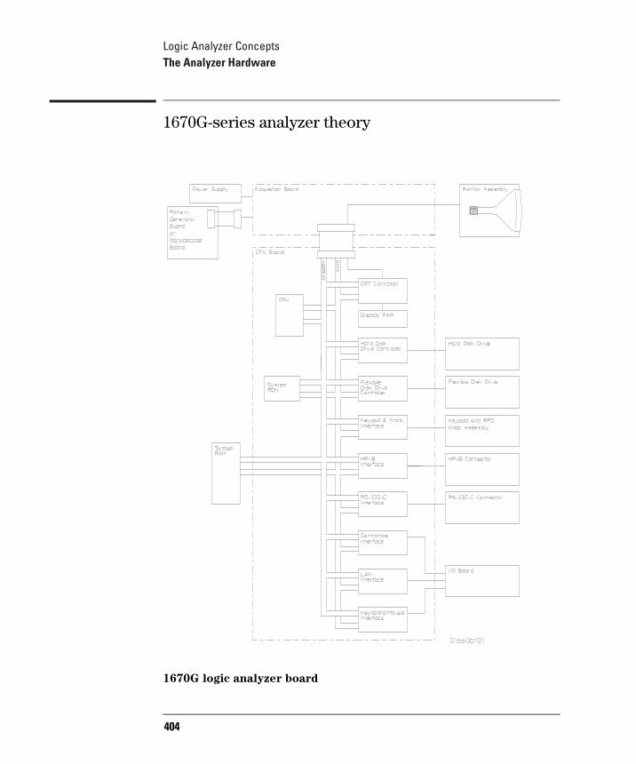
Logic Analyzer ConceptsThe Analyzer Hardware
1670G-series analyzer theory
1670G logic analyzer board
404
Logic Analyzer ConceptsThe Analyzer Hardware
CPU board
The microprocessor is a Motorola 68EC020 running at 25 MHz. The microprocessor controls all of the functions of the logic analyzer including processing and storing data, displaying data, and configuring the acquisition ICs to obtain and store data.
System memory
The system memory is made up of both read-only memory (ROM) and random access memory (RAM). Two types of ROM are used. A single 128Kx8 EPROM is used as a boot ROM, and four 512Kx8 Flash ROMs are configured to provide a 512Kx32 Flash ROM space. One SIMM socket supports 2-MB, 4-MB, or 8-MB SIMMs.
On power-up, instructions in the boot ROM command the instrument to execute its boot routine. The boot routine includes power-up operation verification of the instrument subsystems and entering the operating system. The CPU searches for the operating system on flash ROM. Then, if the operating system is in flash ROM, the instrument will be initialized with the default configuration and await front panel instructions from you. If the operating system is not in flash ROM, the CPU accesses the disk drives to see if the operating system is on the disks.
The DRAM stores the instrument configuration, acquired data to be processed, and any inverse assembler loaded in the instrument by the user.
Keypad and knob interface
The front panel keypad is scanned directly from the microprocessor address bus during the video blanking cycle of the CRT. When a front panel key is pressed the associated address bits are fed to the data bus through the pressed key and read by the microprocessor.
The rotary pulse generator (RPG) knob has its own interface. Pulses and direction of rotation information are directed to the RPG interface. The microprocessor then reads and interprets the RPG signals and performs the desired tasks.
405
Logic Analyzer ConceptsThe Analyzer Hardware
GPIB interface
The instrument interfaces to GPIB as defined by IEEE Standard 488.2. The interface consists of an GPIB controller and two octal drivers/receivers. The microprocessor routes GPIB data to the controller. The controller then buffers the 8-bit GPIB data bits and generates the bus handshaking signals. The data and handshaking signals are then routed to the GPIB bus through the octal line drivers/receivers. The drivers/receivers provide data and control signal transfer between the bus and controller.
RS-232-C interface
The instrument RS-232-C interface is compatible with standard RS-232-C protocol. The interface consists of a controller and drivers/receivers. The controller serializes parallel data from the microprocessor for transmission. At the same time the controller also receives serial data and converts the data to parallel data characters for the microprocessor.
The controller contains a baud rate generator that can be programmed from the logic analyzer front panel. Other RS-232-C communications parameters can also be programmed from the logic analyzer front panel.
The drivers/receivers interface the instrument with data communications equipment. Slew rate control is provided on the ICs eliminating the need for external capacitors.
Power supply
A low voltage power supply provides all dc voltages needed to operate the logic analyzer. The power supply also provides the +5 V dc voltage to the probe cables to power logic analyzer accessories and analysis probes.
Unfiltered voltages of +12 V, -12 V, +5 V, -5.2 V, and +3.5 V are supplied to the acquisition board where they are filtered and distributed to the CPU board, CRT Monitor Assembly, and probe cables.
406
Logic Analyzer ConceptsThe Analyzer Hardware
LAN Interface
The LAN Interface is primarily a single LAN integrated circuit with supporting components. Isolation circuitry for the LAN port is included on the I/O board. The LAN interface conforms to IEEE 802.3
407
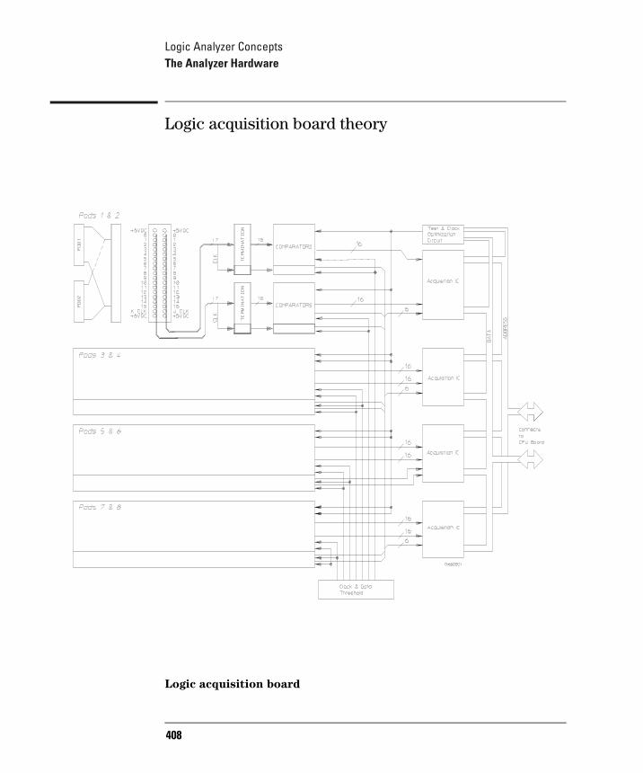
Logic Analyzer ConceptsThe Analyzer Hardware
Logic acquisition board theory
Logic acquisition board
408
Logic Analyzer ConceptsThe Analyzer Hardware
Probing
The probing circuit includes the probe cable and terminations. The probe cable consists of two 17-channel pods which are connected to the circuit board using a high-density connector. Sixteen single-ended data channels and one single-ended clock/data channel per pod are passed to the circuit board. If the clock/data channel is not used as a state clock in state acquisition mode, it is available as a data channel. The clock/data channel is also available as a data channel in timing acquisition mode. Eight (1670’s), six (1671’s), four (1672’s), or two (1673’s) clock/data channels are available as data channels; however, only four clock/data channels can be assigned as clock channels in the 1670’s, 1671’s, and 1672’s. In the 1673’s, only two clock/data channels can be assigned as clock channels.
The cables use nichrome wire woven in polyarmid yarn for reliability and durability. The pods also include one ground path per channel in addition to a pod ground. The channel grounds are configured such that their electrical distance is the same as the electrical distance of the channel. The probe tip assemblies and termination modules connected at the end of the probe cables have a divide-by-10 RC network that reduces the amplitude of the data signals as seen by the circuit board. This adds flexibility to the types of signals the circuit board can read in addition to improving signal integrity.
The terminations on the circuit board are resistive terminations that reduce transmission line effects on the cable. The terminations also improve signal integrity to the comparators by matching the impedance of the probe cable channels with the impedance of the signal paths of the circuit board. All 17 channels of each pod are terminated in the same way. The signals are reduced by a factor of 10.
Comparators
Two proprietary 9-channel comparators per pod interpret the incoming data and clock signals as either high or low depending on where the user- programmable threshold is set. The threshold voltage of each pod is individually programmed, and the voltage selected applies to the clock channel as well as the data channels of each pod.
Each of the comparator ICs has a serial test input port used for testing
409
Logic Analyzer ConceptsThe Analyzer Hardware
purposes. A test bit pattern is sent from the Test and Clock Synchronization Circuit to the comparator. The comparators then propagate the test signal on each of the nine channels of the comparator. Consequently, all data and clock channel pipelines on the circuit board can be tested by the operating system software from the comparator.
Acquisition
The acquisition circuit is made up of a single Agilent-proprietary ASIC. Each ASIC is a 34-channel state/timing analyzer, and one such ASIC is included for every two logic analyzer pods. All of the sequencing, pattern/range recognition, and event counting functions are performed on board the IC.
In addition to the storage qualification and counting functions, the acquisition ASICs also perform master clocking functions. All four state acquisition clocks are fed to each IC, and the ICs generate their own sample clocks. Every time you select run, the ICs individually perform a clock optimization before data is stored.
Clock optimization involves using programmable delays on board the IC to position the master clock transition where valid data is captured. This procedure greatly reduces the effects of channel-to-channel skew and other propagation delays.
In the timing acquisition mode, an oscillator-driven clock circuit provides a four-phase, 125-MHz clock signal to each of the acquisition ICs. For high speed timing acquisition (125 MHz and faster), the sample period is determined by the four-phase, 125-MHz clock signal.
For slower sample rates, one of the acquisition ICs divides the 125-MHz clock signal to the appropriate sample rate. The sample clock is then fed to all acquisition ICs.
410
Logic Analyzer ConceptsThe Analyzer Hardware
Threshold
A precision octal DAC and precision op amp drivers make up the threshold circuit. Each of the eight channels of the DAC is individually programmable which allows you to set the thresholds of the individual pods. The 16 data channels and the clock channel of each pod are all set to the same threshold voltage.
Test and clock synchronization circuit
ECLinPS ICs are used in the test and clock synchronization circuit for reliability and low channel-to-channel skew. Test patterns are generated and sent to the comparators during software operation verification. The test patterns are propagated across all data and clock channels and read by the acquisition ASIC to ensure both the data and clock pipelines are operating correctly.
The test and clock synchronization circuit also generates a four-phase, 125-MHz sample/synchronization signal for the acquisition ICs operating in the timing acquisition mode. The synchronizing signal keeps the internal clocking of the individual acquisition ASICs locked in step with the other ASICs at fast sample rates. At slower sample rates, one of the acquisition ICs divides the 125-MHz clock signal to the appropriate sample rate. The slow speed sample clock is then used by all acquisition ICs.
411
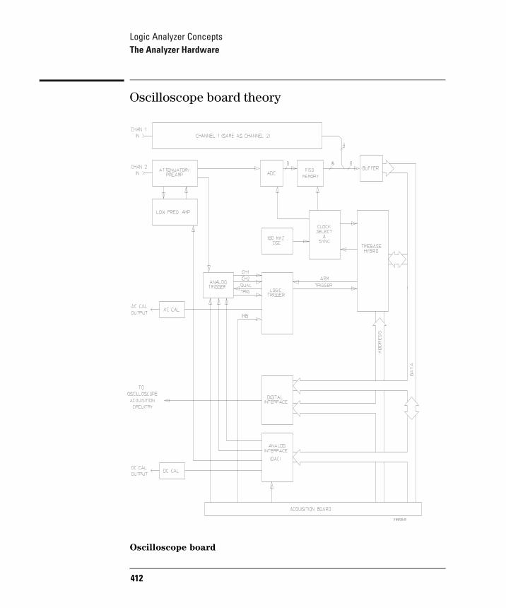
Logic Analyzer ConceptsThe Analyzer Hardware
Oscilloscope board theory
Oscilloscope board
412
Logic Analyzer ConceptsThe Analyzer Hardware
Attenuator/Preamp theory of operation
The channel signals are conditioned by the attenuator/preamps, thick film hybrids containing passive attenuators, impedance converters, and a programmable amplifier. The channel sensitivity defaults to the standard 1-2-4 sequence (other sensitivities can be set also). However, the firmware uses passive attenuation of 1, 5, 25, and 125, with the programmable preamp, to cover the entire sensitivity range.
The input has a selectable 1 MW input impedance with ac or dc coupling or a 50W input impedance with dc coupling. Compensation for the passive attenuators is laser-trimmed and is not adjustable. After the passive attenuators, the signal is split into high-frequency and low-frequency components. Low frequency components are amplified on the main assembly, where they are combined with the offset voltage. The ac coupling is implemented in the low frequency amplifier.
The high- and low-frequency components of the signal are recombined and applied to the input FET of the preamp. The FET provides a high input impedance for the preamp. The programmable preamp adjusts the gain to suit the required sensitivity and provides the output signal to the main assembly. The output signal is then sent to both the trigger circuitry and ADC.
Oscilloscope acquisition
The acquisition circuitry provides the sampling, digitizing, and storing of the signals from the channel attenuators. The channels are identical. Trigger signals from each channel and the external triggers synchronize acquisition through the time base circuitry. A 100MHz oscillator and a time base provide system timing and sample clocking. A voltage-controlled oscillator (VCO), frequency divider, and digital phase detector provide the sample clock for higher sample rates. After conditioning and sampling, the signals are digitized, then stored in a hybrid IC containing a FISO (fast in, slow out) memory.
413

Logic Analyzer ConceptsThe Analyzer Hardware
ADC Hybrid. The ACD Hybrid provides all of the sampling, digitizing, and high-speed waveform storage. The ADC includes a phase-locked loop frequency converter that, for sample rates from 250 MHz to 2 GHz, multiplies the input clock from the time base.
FISO memory. 32,768 samples of the FISO (fast in, slow out) memory are used per measurement per channel. Memory positions are not addressed directly. The configuration is a ring which loops continuously as it is clocked. Memory position is tracked by counting clocks. The clocking rate is the same as the ADC, however the clock frequency is half that of the ADC since the FISO clocks on both transitions of the clock period. Data is buffered onto the CPU data bus for processing.
Triggering. There are two main trigger circuits that control four trigger sources. The two trigger circuits are the analog trigger and the logic trigger. The analog trigger IC operates as a multichannel Schmidt trigger/comparator. A trigger signal (a copy of the analog input signal) from each of the inputs (channel 1 and channel 2) is directed to the analog trigger IC inputs. The trigger signal is continuously compared with the trigger reference level selected by the user. Once the trigger condition is met, the trigger true signal is fed to the logic trigger, which begins the acquisition and store functions by way of the time base.
The four trigger sources are Channel 1, Channel 2, Intermodule Bus (IMB), and external BNC. Channel 1 and channel 2 triggers were discussed previously. The IMB trigger signal is sent directly to the logic trigger. External triggering is provided by the BNC input of the 1670G-series logic analyzers with the oscilloscope option.
Time base. The time base provides the sample clocks and timing necessary for data acquisition. It consists of the 100 MHz reference oscillator and time base hybrid.
414
Logic Analyzer ConceptsThe Analyzer Hardware
The 100 MHz reference oscillator provides the base sample frequency. The time base hybrid has programmable dividers to provide the rest of the sample frequencies appropriate for the time range selected. The time base uses the time-stretched output of the fine interpolator to time-reference the sampling to the trigger point. The time base has counters to control how much data is taken before (pre-trigger data) and after (post-trigger data) the trigger event. After the desired number of pre-trigger samples has occurred, the time base hybrid sends a signal to the logic trigger (trigger arm) indicating it is ready for the trigger event. When the trigger condition is satisfied, the logic trigger sends a signal back to the time base hybrid. The time base hybrid then starts the post-trigger delay counter.
When the countdown reaches zero, the sample clocks are stopped and the CPU is signaled that the acquisition is complete. The fine interpolator is a dual-slope integrator that acts as a time-interval stretcher. When the logic trigger receives a signal that meets the programmed triggering requirements, it signals the time base. The time base then sends a pulse to the fine interpolator. The pulse is equal in width to the time between the trigger and the next sample clock. The fine interpolator stretches this time by a factor of approximately 500. Meanwhile, the time base hybrid runs a counter with a clock derived from the sample rate oscillator. When the interpolator indicates the stretch is complete, the counter is stopped. The count represents, with much higher accuracy, the time between the trigger and the first sample clock. The count is stored and used to place the recently acquired data in relationship with previous data.
AC/DC Cal. The AC Cal is a multiplexer circuit that can provide several signals to the Probe Compensation/AC Calibrator output on the rear panel. The signal provided depends on the mode of the instrument. It can be either a probe compensation signal, a pulse representing the trigger event, signals used for self-calibration, or the 100 MHz reference oscillator when sample period is 1 ns. The DC Cal output, a rear panel signal, is used for self-calibration. It is one output from the 16-channel DAC.
415
Logic Analyzer ConceptsThe Analyzer Hardware
Digital Interface. The Digital Interface provides control and interface between the system control and digital functions in the acquisition circuitry.
Analog Interface
The Analog Interface provides control of analog functions in the acquisition circuitry. It is primarily a 16-channel DAC with an accurate reference and filters on the outputs. It controls channel offsets and trigger levels, and provides the DC Cal output.
416
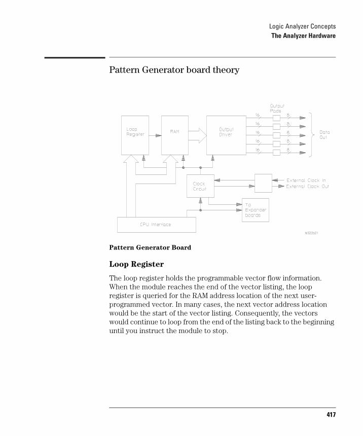
Logic Analyzer ConceptsThe Analyzer Hardware
Pattern Generator board theory
Pattern Generator Board
Loop Register
The loop register holds the programmable vector flow information. When the module reaches the end of the vector listing, the loop register is queried for the RAM address location of the next user-programmed vector. In many cases, the next vector address location would be the start of the vector listing. Consequently, the vectors would continue to loop from the end of the listing back to the beginning until you instruct the module to stop.
417
Logic Analyzer ConceptsThe Analyzer Hardware
RAM
Consisting of five 256Kx16 VRAM ICs and RAM addressing circuitry, the RAM stores the desired patterns that appear at the module output. The RAM addressing circuitry is merely a counter which addresses the pattern locations in RAM. When the end of the vector listing is reached, the addressing circuitry is loaded from the loop register with the address of the first vector of the listing to provide an uninterrupted vector loop. The RAM output is sent to the Output Driver circuit where the patterns are presented in a logic configuration usable by the output pods.
Output Driver
The output driver circuit is made up of a series of latch/logic translators and multiplexers. The latch/translators convert the working-level TTL signals to output-level ECL signals for each channel. The ECL-level signals are then directed to the multiplexers.
The multiplexers, one per channel, direct the programmed data patterns to the output channels. The single-ended ECL-level signals are converted to differential signals which are routed to the output cables and to the pods. Note that the differential ECL output signal of the pattern generator module is not suitable to directly drive ECL circuitry.
Clock Circuit
The clock circuit paces the loop register, the RAM address circuitry, and the multiplexers in the output driver according to the desired data rate. A 200 MHz clock source is directed through a divider circuit which provides a 100 MHz and 50 MHz clock in addition to 200 MHz. The 200 MHz, 100 MHz, 50 MHz and external clock signals are routed to a clock select multiplexer. The output of the multiplexer, which represents the user-selected clocking rate, is distributed to the above listed subcircuits.
418
Logic Analyzer ConceptsThe Analyzer Hardware
The output of the clock select multiplexer is also distributed to an external clock out circuit. The clock signal is routed to a bank of external clock delays, and then to an external clock delay select multiplexer. The output of this multiplexer, which represents the desired clock delay, is directed to the external clock out pin on the clock pod. Consequently, either the internal clock or external clock is redirected to the clock out pin on the clock pod with a user-selected clock delay.
CPU Interface
The CPU interface is a single programmable-logic device which interprets the 1670EP Logic Analysis System backplane logic and translates the logic into signals to drive and program the pattern generator module.
Pod
The Clock or Data Pod converts the differential output ECL signal to the logic levels of interest. Because the output of the pattern generator module cannot directly drive ECL circuitry, the Clock and Data Pod is required to interface the pattern generator with the target system.
419

Logic Analyzer ConceptsThe Analyzer Hardware
Self-tests description
The self-tests identify the correct operation of major functional areas in the logic analyzer. The self-tests are not intended for component-level diagnostics.
Three types of tests are performed on the 1670G-series logic analyzers: the power-up self-tests, the functional performance verification self-tests, and the parametric performance verification tests.
The power-up self-tests are performed when power is applied to the instrument. The power-up self-tests are divided into two parts. The first part is the system memory tests and the second part is the microprocessor interrupt test. The system memory tests are performed before the logic analyzer actually displays the power-up self-test screen. Both the system ROM and RAM are tested during power-up. The interrupt test is performed after the power-up self-test screen is displayed.
The functional performance verification self-tests are run using a separate operating system, the performance verification (PV) operating system. The PV operating system resides on a separate disk that must be loaded when running the functional performance verification self-tests. The system and analyzer tests are functional performance verification tests.
Parametric performance verification requires the use of external test equipment that generates and monitors test data for the logic analyzer to read. Refer to the Agilent Technologies 1670G-Series Logic Analyzers Service Guide for further information about parametric performance verification.
420

12
Troubleshooting the Logic Analyzer
421

Troubleshooting the Logic AnalyzerTroubleshooting the Logic Analyzer
Troubleshooting the Logic AnalyzerOccasionally, a measurement may not give the expected results. If you encounter difficulties while making measurements, use this chapter to guide you through some possible solutions. Each heading lists a problem you may encounter, along with some possible solutions. Error messages which may appear on the logic analyzer are listed below in quotes " ". Symptoms are listed without quotes.
If you still have difficulty using the analyzer after trying the suggestions in this chapter, please contact your local Agilent Technologies Service Center.
CAUTION: When you are working with the analyzer, be sure to power down both the analyzer and the target system before disconnecting or connecting cables, probes, and analysis probes. Otherwise, you may damage circuitry in the analyzer, analysis probe, or target system.
422
Troubleshooting the Logic AnalyzerAnalyzer Problems
Analyzer ProblemsThis section lists general problems that you might encounter while using the analyzer.
Intermittent data errors
This problem is usually caused by poor connections, incorrect signal levels, or marginal timing.
With the logic analyzer and all connected equipment turned off, remove and reseat all cables and probes; ensure that there are no bent pins on the analysis probe or poor probe connections.
Adjust the threshold level of the data pod in the Format menu to match the logic levels in the system under test.
Use an oscilloscope to check the signal integrity of the data lines.
Clock signals for the state analyzer must meet particular pulse shape and timing requirements. Data inputs for the analyzer must meet pulse shape and setup and hold time requirements.
See Also "Capacitive loading" in this section for information on other sources of intermittent data errors.
423
Troubleshooting the Logic AnalyzerAnalyzer Problems
Unwanted triggers
Unwanted triggers can be caused by instructions that were fetched but not executed.
Add the prefetch queue or pipeline depth to the trigger address.
The depth of the prefetch queue depends on the processor that you are analyzing. Suppose you are analyzing a pipelined processor having fetch, decode, execute, and memory stages. The processor fetches 32-bit words. To ensure that the processor has begun executing a particular routine when the trigger occurs, set the trigger to the module entry address plus 08 hex. (This assumes that there is no immediate data in the instruction stream.)
No activity on activity indicators
Ensure that the Threshold settings in the Format menu match the logic family being probed.
Check for loose cables, board connections, and analysis probe connections.
Check for bent or damaged pins on the analysis probe.
424

Troubleshooting the Logic AnalyzerAnalyzer Problems
Capacitive loading
Excessive capacitive loading can degrade signals, resulting in incorrect capture by the analysis probe, or system lockup in the microprocessor. All analysis probes add additional capacitive loading, as can custom probe fixtures you design for your application. To reduce loading, remove as many pin protectors, extenders, and adapters as possible.
Careful layout of your target system can minimize loading problems and result in better margins for your design. This is especially important for systems that are running at frequencies greater than 50 MHz.
No trace list display
If there is no trace list display, it may be that your trigger specification is not correct for the data you want to capture, or that the trace memory is only partially filled.
Check your trigger specification to ensure that it will capture the events of interest.
Try stopping the analyzer; if the trace list is partially filled, this should display the contents of trace memory.
425

Troubleshooting the Logic AnalyzerAnalysis Probe Problems
Analysis Probe ProblemsThis section lists problems that you might encounter when using an analysis probe. If the solutions suggested here do not correct the problem, you may have a defective analysis probe. Refer to the User's Guide for your analysis probe for test procedures. Contact your local Agilent Technologies Sales Office if you need further assistance.
Target system will not boot up
If the target system will not boot up after connecting the analysis probe, the microprocessor or the analysis probe may not be installed properly, or they may not be making electrical contact.
Ensure that you are following the correct power-on sequence for the analysis probe and target system. 1. Power up the analyzer and analysis probe.2. Power up the target system.
If you power up the target system before you power up the analysis probe, interface circuitry in the analysis probe may latch up, preventing proper target system operation.
Verify that the microprocessor and the analysis probe are properly rotated and aligned, so that the index pin on the microprocessor (such as pin 1 or A1) matches the index pin on the analysis probe.
Verify that the microprocessor and the analysis probe are securely inserted into their respective sockets.
Verify that the logic analyzer cables are in the proper sockets of the analysis probe and are firmly inserted.
Reduce the number of extender sockets.
See Also "Capacitive loading" in the previous section of this chapter.
426
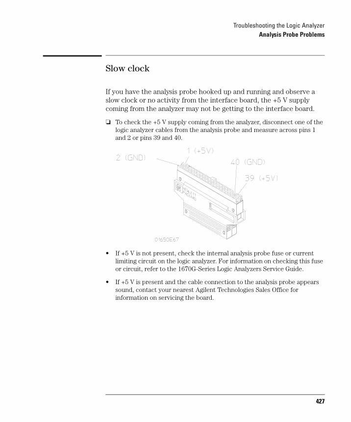
Troubleshooting the Logic AnalyzerAnalysis Probe Problems
Slow clock
If you have the analysis probe hooked up and running and observe a slow clock or no activity from the interface board, the +5 V supply coming from the analyzer may not be getting to the interface board.
To check the +5 V supply coming from the analyzer, disconnect one of the logic analyzer cables from the analysis probe and measure across pins 1 and 2 or pins 39 and 40.
• If +5 V is not present, check the internal analysis probe fuse or current limiting circuit on the logic analyzer. For information on checking this fuse or circuit, refer to the 1670G-Series Logic Analyzers Service Guide.
• If +5 V is present and the cable connection to the analysis probe appears sound, contact your nearest Agilent Technologies Sales Office for information on servicing the board.
427

Troubleshooting the Logic AnalyzerAnalysis Probe Problems
Erratic trace measurements
There are several general problems that can cause erratic variations in trace lists and inverse assembly failures.
Ensure that the analysis probe configuration switches are correctly set for the measurement you are trying to make.Some analysis probes include configuration switches for various features (for example, to allow dequeueing of the trace list). See your Analysis Probe User's Guide for more information.
Try doing a full reset of the target system before beginning the measurement.Some analysis probe designs require a full reset to ensure correct configuration.
Ensure that your target system meets the timing requirements of the processor with the analysis probe installed.See "Capacitive loading" in this chapter. While analysis probe loading is slight, pin protectors, extenders, and adapters may increase it to unacceptable levels. If the target system design has poor timing margins, such loading may cause incorrect processor functioning, giving erratic trace results.
Ensure that you have sufficient cooling for the analysis probe.Current processors such as the i486, Pentiumø, and MC68040 generate substantial heat. This is exacerbated by the active circuitry on the analysis probe. You should ensure that you have ambient temperature conditions and airflow that meet or exceed the requirements of the microprocessor manufacturer.
428
Troubleshooting the Logic AnalyzerInverse Assembler Problems
Inverse Assembler ProblemsThis section lists problems that you might encounter while using the inverse assembler.
When you obtain incorrect inverse assembly results, it may be unclear whether the problem is in the analysis probe or in your target system. If you follow the suggestions in this section to ensure that you are using the analysis probe and inverse assembler correctly, you can proceed with confidence in debugging your target system.
No inverse assembly or incorrect inverse assembly
This problem is due to incorrect synchronization, modified configuration, incorrect connections, or a hardware problem in the target system. A locked status line can cause incorrect or incomplete inverse assembly.
Verify that the inverse assembler has been synchronized by placing an opcode at the top of the display (not at the input cursor) and pressing the Invasm key.Because the inverse assembler works from the first line of the trace display, if you jump to the middle of a trace and select Invasm, prior trace states are not disassembled correctly. If you move to several random places in the trace list and select Invasm each time, the trace disassembly is only guaranteed to be correct from the top of the display forward for each selection.
See Also "The Inverse Assembler" on page 65.
429
Troubleshooting the Logic AnalyzerInverse Assembler Problems
Ensure that each analyzer pod is connected to the correct analysis probe cable.There is not always a one-to-one correspondence between analyzer pod numbers and analysis probe cable numbers. Analysis probes must supply address (ADDR), data (DATA), and status (STAT) information to the analyzer in a predefined order, so the cable connections for each analysis probe are often altered to support that need. Thus, one analysis probe might require that you connect cable 2 to analyzer pod 2, while another will require you to connect cable 5 to analyzer pod 2. See the User's Guide for your analysis probe for further information.
Check the activity indicators for status lines locked in a high or low state.
Verify that the STAT, DATA, and ADDR format labels have not been modified from their default values.These labels must remain as they are configured by the configuration file. Do not change the names of these labels or the bit assignments within the labels. Some analysis probes also require other data labels; check your Analysis Probe User's Guide for more information.
Verify that all microprocessor caches and memory managers have been disabled.In most cases, if the microprocessor caches and memory managers remain enabled you should still get inverse assembly, but it may be incorrect since some of the execution trace was not visible to the logic analyzer.
Verify that storage qualification has not excluded storage of all the needed opcodes and operands.
430
Troubleshooting the Logic AnalyzerInverse Assembler Problems
Inverse assembler will not load or run
You need to ensure that you have the correct system software loaded on your analyzer.
Ensure that the inverse assembler is on the same disk as the configuration files you are loading.Configuration files for the state analyzer contain a pointer to the location of the corresponding inverse assembler. If you delete the inverse assembler or move it to another location, the configuration process will fail.
Make sure you are using the version of the inverse assembler software that corresponds to the operating system revision installed on your analyzer.See your Analysis Probe User's Guide for details.
431

Troubleshooting the Logic AnalyzerError Messages
Error MessagesThis section lists some of the messages that the analyzer displays when it encounters a problem.
". . . Inverse Assembler Not Found"
This error occurs if you rename or delete the inverse assembler file that is attached to the configuration file. Ensure that the inverse assembler file is not renamed or deleted, and that it is on the same flexible disk or in the same directory as the configuration file.
"No Configuration File Loaded"
This is usually caused by trying to load a configuration file for one type of module or the system into a different type of module.
Verify that the appropriate module has been selected as the target of the Load operation. Selecting Load All will cause incorrect operation when loading most analysis probe configuration files.
See Also "To Load a Configuration" on page 137.
432
Troubleshooting the Logic AnalyzerError Messages
"Selected File is Incompatible"
This occurs when you try to load a configuration file for the wrong module. Ensure that you are loading a translatable configuration file for your logic analyzer.
"Slow or Missing Clock"
This error might occur if the target system is not running properly. Ensure that the target system is on and operating properly.
Check your State clock configuration. The proper clocking scheme should be listed in your Analysis Probe User's Guide.
If the error message persists, check that the logic analyzer pods are connected to the proper connectors. See the User's Guide for your analysis probe to determine the proper connections.
"Waiting for Trigger"
If a trigger pattern is specified, this message indicates that the specified trigger pattern has not occurred. Verify that the triggering pattern is correctly set.
When analyzing microprocessors that fetch only from long-word aligned addresses, if the trigger condition is set to look for an opcode fetch at an address not corresponding to a long-word boundary, the trigger will never be found.
433
Troubleshooting the Logic AnalyzerError Messages
"Must have at least 1 edge specified"
You must assign at least one clock edge to one of the available clocks in the clocking arrangement. The analyzer will not let you close the clock assignment pop-up until an edge is specified.
"Time correlation of data is not possible"
To time-correlate data, the data must be stored with time tags.
Set the Count field in the Analyzer Trigger menu to Time.
"Maximum of 32 channels per label"
You have tried to assign more than 32 channels to a single label.
Unassign some of the channels. If you need more than 32 channels to specify trigger conditions, you can AND terms in the Analyzer Trigger menu.
434
Troubleshooting the Logic AnalyzerError Messages
"Timer is off in sequence level n where it is used"
If you use timers as part of your trigger sequence, you must remember to turn them on using Timer Control in the Sequence Level pop-up menu.
Check that your timers are turned on. The timer status is shown in the right side of the Sequence Level display of the Trigger menu. An "S" means "Start", "P" means "Pause", "C" means "Continue", and "-" means "off".
"Timer is specified in sequence, but never started"
This message often appears with "Timer is off in sequence level n where it is used," but is not quite the same. That message refers to a particular sequence level, but this message is a general warning that the timer has not been set to Start in any level.
Start the timer in one of the levels before where it is used.
"Inverse assembler not loaded - bad object code."
The inverse assembler file has been corrupted.
Try loading a different copy of the inverse assembler.
435
Troubleshooting the Logic AnalyzerError Messages
"Measurement Initialization Error"
The logic analyzer failed its internal hardware calibration.
Run the Performance Verification tests.
See Also The Agilent Technologies 1670G-Series Logic Analyzers Service Guide for information on running the Performance Verification test.
"Warning: Run HALTED due to variable change"
This message appears when certain analyzer settings are changed during a repetitive run. When this occurs, the analyzer stops.
436

13
Specifications
437
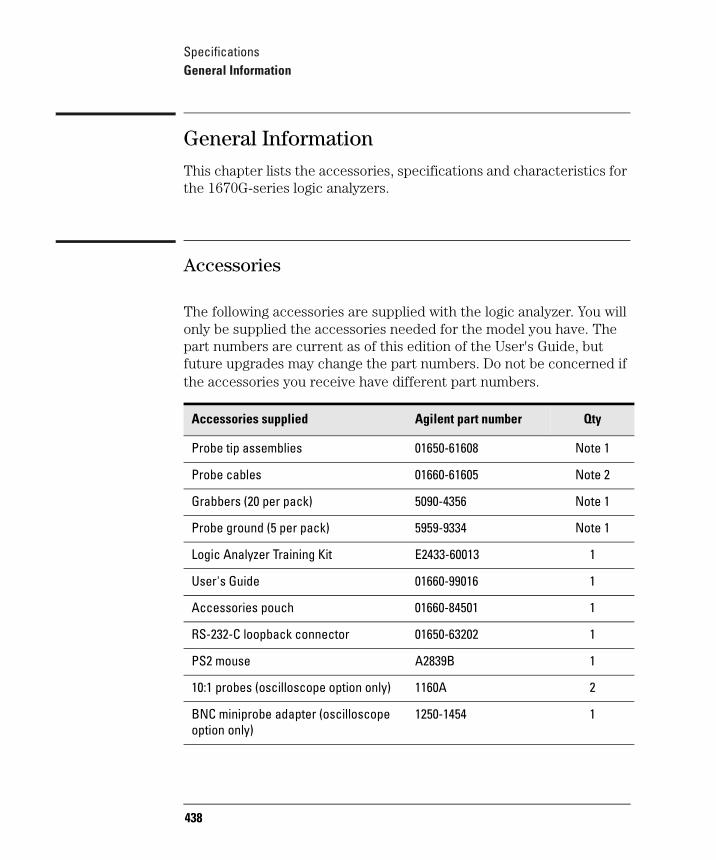
SpecificationsGeneral Information
General InformationThis chapter lists the accessories, specifications and characteristics for the 1670G-series logic analyzers.
Accessories
The following accessories are supplied with the logic analyzer. You will only be supplied the accessories needed for the model you have. The part numbers are current as of this edition of the User's Guide, but future upgrades may change the part numbers. Do not be concerned if the accessories you receive have different part numbers.
Accessories supplied Agilent part number Qty
Probe tip assemblies 01650-61608 Note 1
Probe cables 01660-61605 Note 2
Grabbers (20 per pack) 5090-4356 Note 1
Probe ground (5 per pack) 5959-9334 Note 1
Logic Analyzer Training Kit E2433-60013 1
User's Guide 01660-99016 1
Accessories pouch 01660-84501 1
RS-232-C loopback connector 01650-63202 1
PS2 mouse A2839B 1
10:1 probes (oscilloscope option only) 1160A 2
BNC miniprobe adapter (oscilloscope option only)
1250-1454 1
438

SpecificationsGeneral Information
Note 1 Quantities: 8 - 1670G6 - 1671G4 - 1672G2 - 1673G
Note 2 Quantities 4 - 1670G3 - 1671G2 - 1672G1 - 1673G
439
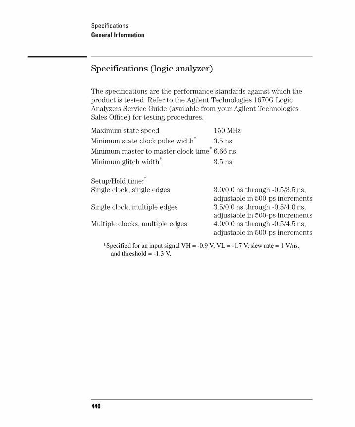
SpecificationsGeneral Information
Specifications (logic analyzer)
The specifications are the performance standards against which the product is tested. Refer to the Agilent Technologies 1670G Logic Analyzers Service Guide (available from your Agilent Technologies Sales Office) for testing procedures.
Maximum state speed 150 MHz
Minimum state clock pulse width* 3.5 ns
Minimum master to master clock time* 6.66 ns
Minimum glitch width* 3.5 ns
Setup/Hold time:*
Single clock, single edges 3.0/0.0 ns through -0.5/3.5 ns,adjustable in 500-ps increments
Single clock, multiple edges 3.5/0.0 ns through -0.5/4.0 ns,adjustable in 500-ps increments
Multiple clocks, multiple edges 4.0/0.0 ns through -0.5/4.5 ns,adjustable in 500-ps increments
*Specified for an input signal VH = -0.9 V, VL = -1.7 V, slew rate = 1 V/ns, and threshold = -1.3 V.
440
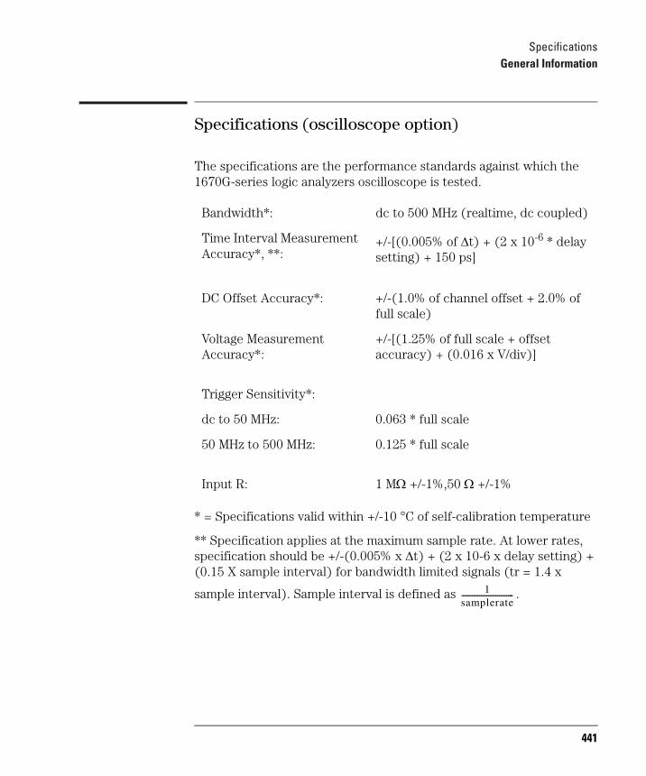
SpecificationsGeneral Information
Specifications (oscilloscope option)
The specifications are the performance standards against which the 1670G-series logic analyzers oscilloscope is tested.
* = Specifications valid within +/-10 °C of self-calibration temperature
** Specification applies at the maximum sample rate. At lower rates, specification should be +/-(0.005% x ∆t) + (2 x 10⁻⁶ x delay setting) + (0.15 X sample interval) for bandwidth limited signals (tr = 1.4 x
sample interval). Sample interval is defined as .
Bandwidth*: dc to 500 MHz (realtime, dc coupled)
Time Interval Measurement Accuracy*, **:
+/-[(0.005% of ∆t) + (2 x 10⁻⁶ * delay setting) + 150 ps]
DC Offset Accuracy*: +/-(1.0% of channel offset + 2.0% of full scale)
Voltage Measurement Accuracy*:
+/-[(1.25% of full scale + offset accuracy) + (0.016 x V/div)]
Trigger Sensitivity*:
dc to 50 MHz: 0.063 * full scale
50 MHz to 500 MHz: 0.125 * full scale
Input R: 1 MΩ +/-1%,50 Ω +/-1%
1samplerate-----------------------------
441

SpecificationsGeneral Information
Characteristics (logic analyzer)
These characteristics are not specifications, but are included as additional information.
Full Channel Half ChannelMaximum state clock rate 150 MHz not applicableMaximum conventional timing rate 250 MHz 500 MHzMemory depth 64 K 128 KMemory option 001 256 K 512 KMemory option 002 2 M 4 M
Channel count:
1670G 136 681671G 102 511672G 68 341673G 34 17
442
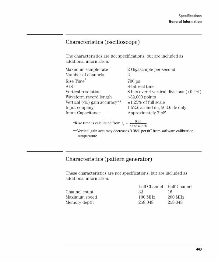
SpecificationsGeneral Information
Characteristics (oscilloscope)
The characteristics are not specifications, but are included as additional information.
Maximum sample rate 2 Gigasample per secondNumber of channels 2
Rise Time* 700 psADC 8-bit real timeVertical resolution 8 bits over 4 vertical divisions (±0.4%)Waveform record length >32,000 pointsVertical (dc) gain accuracy** ±1.25% of full scaleInput coupling 1 MΩ: ac and dc, 50 Ω: dc onlyInput Capacitance Approximately 7 pF
*Rise time is calculated from
**Vertical gain accuracy decreases 0.08% per ûC from software calibration temperature
Characteristics (pattern generator)
These characteristics are not specifications, but are included as additional information.
Full Channel Half ChannelChannel count 32 16Maximum speed 100 MHz 200 MHzMemory depth 258,048 258,048
tr0.35
bandwidth----------------------------=
443
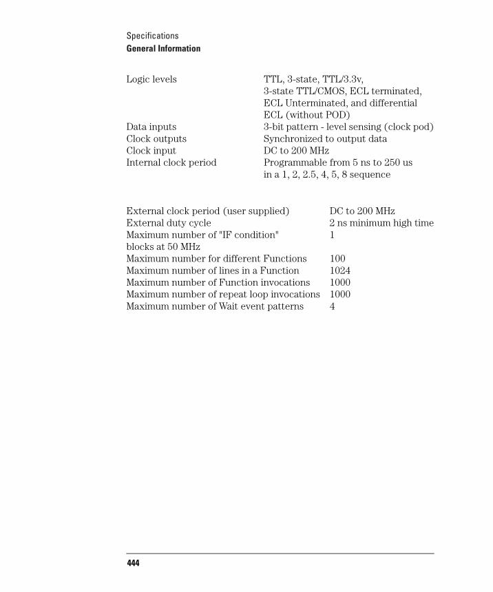
SpecificationsGeneral Information
Logic levels TTL, 3-state, TTL/3.3v, 3-state TTL/CMOS, ECL terminated,ECL Unterminated, and differentialECL (without POD)
Data inputs 3-bit pattern - level sensing (clock pod)Clock outputs Synchronized to output dataClock input DC to 200 MHzInternal clock period Programmable from 5 ns to 250 us
in a 1, 2, 2.5, 4, 5, 8 sequence
External clock period (user supplied) DC to 200 MHzExternal duty cycle 2 ns minimum high timeMaximum number of "IF condition" 1blocks at 50 MHzMaximum number for different Functions 100Maximum number of lines in a Function 1024Maximum number of Function invocations 1000Maximum number of repeat loop invocations 1000Maximum number of Wait event patterns 4
444
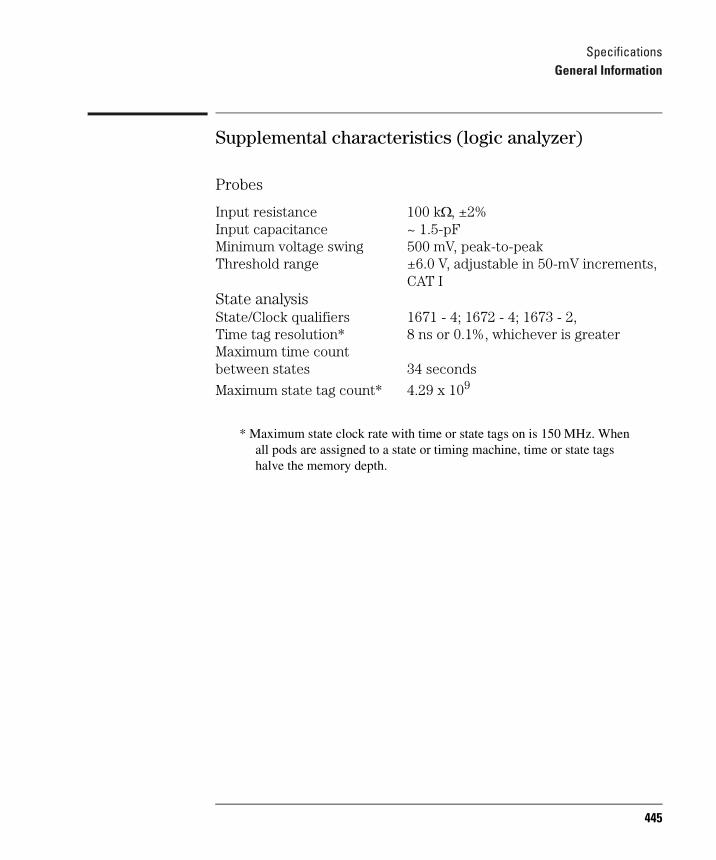
SpecificationsGeneral Information
Supplemental characteristics (logic analyzer)
Probes
Input resistance 100 kΩ, ±2%Input capacitance ~ 1.5-pFMinimum voltage swing 500 mV, peak-to-peakThreshold range ±6.0 V, adjustable in 50-mV increments,
CAT IState analysisState/Clock qualifiers 1671 - 4; 1672 - 4; 1673 - 2, Time tag resolution* 8 ns or 0.1%, whichever is greaterMaximum time count between states 34 seconds
Maximum state tag count* 4.29 x 10⁹
* Maximum state clock rate with time or state tags on is 150 MHz. When all pods are assigned to a state or timing machine, time or state tags halve the memory depth.
445

SpecificationsGeneral Information
Timing analysisSample period accuracy 0.01 % of sample periodChannel-to-channel skew 2 ns, typicalTime interval accuracy ± [sample period + channel-to-channel
skew +(0.01%)(time reading)]
TriggeringSequencer speed 150 MHz, maximumState sequence levels 12Timing sequence levels 10Maximum occurrence counter value 1,048,575Pattern recognizers 10Maximum pattern width 136 channels in 1670G,
102 channels in 1671G, 68 channels in 1672G, 34 channels in 1673G
Range recognizers 2Range width 32 bits eachTimers 2Timer value range 400 ns to 500 secondsGlitch/Edge recognizers 2 (timing only)Maximum glitch/edge width 136 channels in 1670G,
102 channels in 1671G, 68 channels in 1672G, 34 channels in 1673G
446
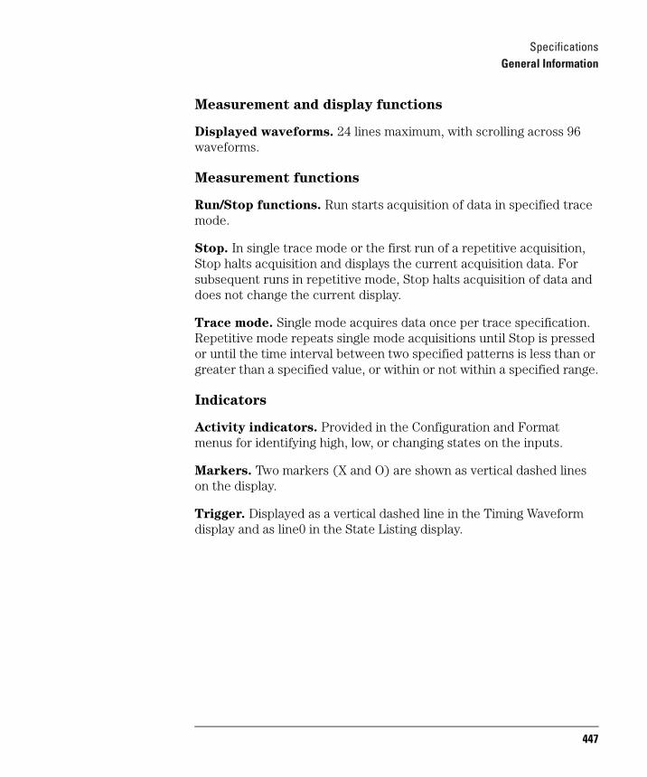
SpecificationsGeneral Information
Measurement and display functions
Displayed waveforms. 24 lines maximum, with scrolling across 96 waveforms.
Measurement functions
Run/Stop functions. Run starts acquisition of data in specified trace mode.
Stop. In single trace mode or the first run of a repetitive acquisition, Stop halts acquisition and displays the current acquisition data. For subsequent runs in repetitive mode, Stop halts acquisition of data and does not change the current display.
Trace mode. Single mode acquires data once per trace specification. Repetitive mode repeats single mode acquisitions until Stop is pressed or until the time interval between two specified patterns is less than or greater than a specified value, or within or not within a specified range.
Indicators
Activity indicators. Provided in the Configuration and Format menus for identifying high, low, or changing states on the inputs.
Markers. Two markers (X and O) are shown as vertical dashed lines on the display.
Trigger. Displayed as a vertical dashed line in the Timing Waveform display and as line0 in the State Listing display.
447
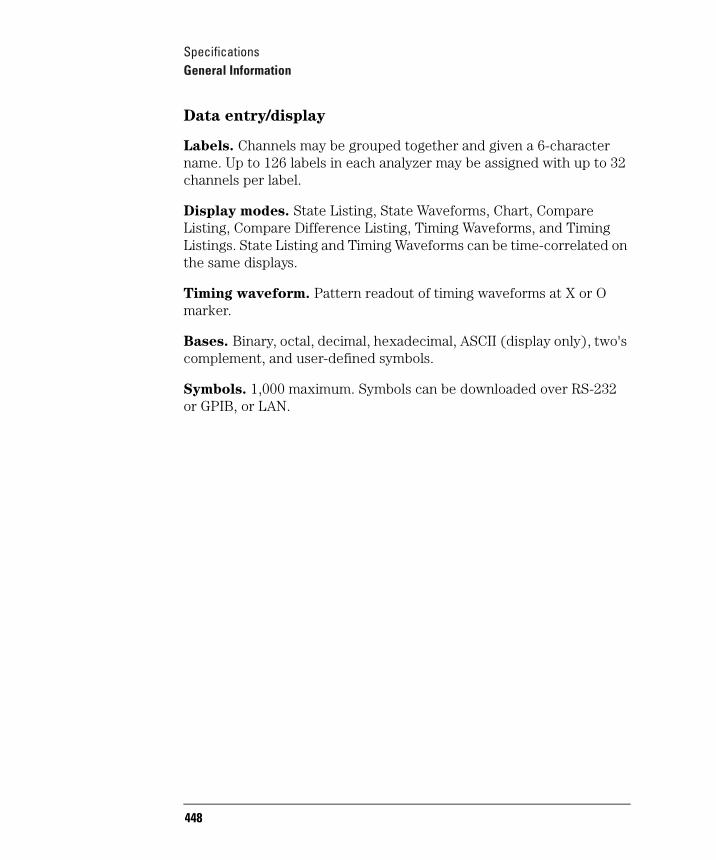
SpecificationsGeneral Information
Data entry/display
Labels. Channels may be grouped together and given a 6-character name. Up to 126 labels in each analyzer may be assigned with up to 32 channels per label.
Display modes. State Listing, State Waveforms, Chart, Compare Listing, Compare Difference Listing, Timing Waveforms, and Timing Listings. State Listing and Timing Waveforms can be time-correlated on the same displays.
Timing waveform. Pattern readout of timing waveforms at X or O marker.
Bases. Binary, octal, decimal, hexadecimal, ASCII (display only), two's complement, and user-defined symbols.
Symbols. 1,000 maximum. Symbols can be downloaded over RS-232 or GPIB, or LAN.
448
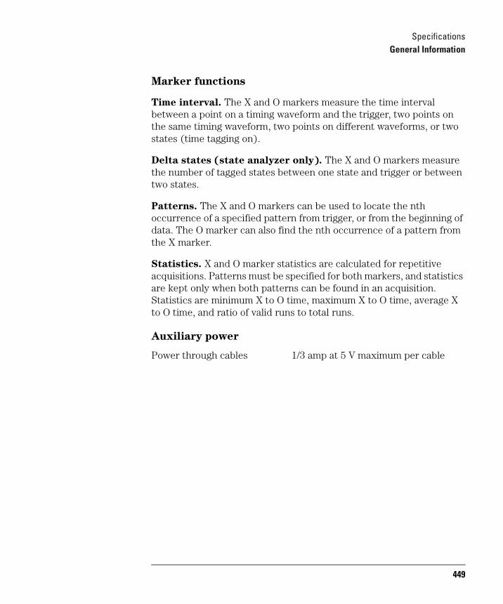
SpecificationsGeneral Information
Marker functions
Time interval. The X and O markers measure the time interval between a point on a timing waveform and the trigger, two points on the same timing waveform, two points on different waveforms, or two states (time tagging on).
Delta states (state analyzer only). The X and O markers measure the number of tagged states between one state and trigger or between two states.
Patterns. The X and O markers can be used to locate the nth occurrence of a specified pattern from trigger, or from the beginning of data. The O marker can also find the nth occurrence of a pattern from the X marker.
Statistics. X and O marker statistics are calculated for repetitive acquisitions. Patterns must be specified for both markers, and statistics are kept only when both patterns can be found in an acquisition. Statistics are minimum X to O time, maximum X to O time, average X to O time, and ratio of valid runs to total runs.
Auxiliary power
Power through cables 1/3 amp at 5 V maximum per cable
449
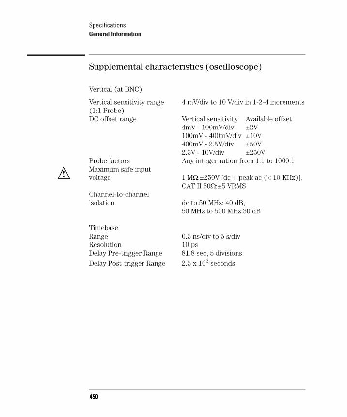
SpecificationsGeneral Information
Supplemental characteristics (oscilloscope)
Vertical (at BNC)
Vertical sensitivity range 4 mV/div to 10 V/div in 1-2-4 increments(1:1 Probe)DC offset range Vertical sensitivity Available offset
4mV - 100mV/div ±2V100mV - 400mV/div ±10V400mV - 2.5V/div ±50V2.5V - 10V/div ±250V
Probe factors Any integer ration from 1:1 to 1000:1Maximum safe input voltage 1 MΩ:±250V [dc + peak ac (< 10 KHz)],
CAT II 50Ω:±5 VRMSChannel-to-channelisolation dc to 50 MHz: 40 dB,
50 MHz to 500 MHz:30 dB
TimebaseRange 0.5 ns/div to 5 s/divResolution 10 psDelay Pre-trigger Range 81.8 sec, 5 divisions
Delay Post-trigger Range 2.5 x 10³ seconds
!
450
SpecificationsGeneral Information
Triggering:
Trigger Level Range: Within display window (vertical offset +/- 2 divisions)
Trigger Modes:
Immediate: Triggers immediately after arming condition is met.
Edge: Triggers on rising or falling edge from channel 1 or channel 2.
Pattern: Triggers on entering or exiting a specified pattern across two channels.
Auto Trigger: Self-triggers if no trigger condition is found within approximately 50 ms after arming.
Events Delay: The trigger can be set to occur on the nth edge or pattern, as specified by the user.
Intermodule: Arms another measurement module or triggers the rear panel BNC.
451
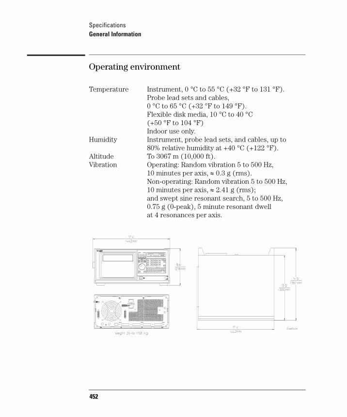
SpecificationsGeneral Information
Operating environment
Temperature Instrument, 0 °C to 55 °C (+32 °F to 131 °F).Probe lead sets and cables, 0 °C to 65 °C (+32 °F to 149 °F).Flexible disk media, 10 °C to 40 °C (+50 °F to 104 °F)Indoor use only.
Humidity Instrument, probe lead sets, and cables, up to80% relative humidity at +40 °C (+122 °F).
Altitude To 3067 m (10,000 ft).Vibration Operating: Random vibration 5 to 500 Hz,
10 minutes per axis, ≈ 0.3 g (rms).Non-operating: Random vibration 5 to 500 Hz,10 minutes per axis, ≈ 2.41 g (rms);and swept sine resonant search, 5 to 500 Hz,0.75 g (0-peak), 5 minute resonant dwell at 4 resonances per axis.
452
14
Operator’s Service
453
Operator’s ServiceOperator’s Service
Operator’s ServiceThis chapter provides information on how to prepare the logic analyzer for use, and contains self-tests and flow charts used for troubleshooting the logic analyzer.
The 1670G-Series Logic Analyzers Service Guide contain detailed service procedures. Service guides can be ordered through your Agilent Technologies Sales Office; they are not shipped with the logic analyzer.
454

Operator’s ServicePreparing For Use
Preparing For UseThis section gives you instructions for preparing the logic analyzer for use.
Power requirements
The logic analyzer requires a power source of either 115 VAC or 230 VAC, -22 % to +10%, single phase, 48 to 66 Hz, 200 Watts maximum power.
Category I: Signal level, telecommunications, electronic. (Seperated from line voltage by transformer, etc).
Category II: Local level, appliances, portable equipment (line voltage in appliance and to wall outlet).
Operating environment
The operating environment is listed in previous chapter. Note the noncondensing humidity limitation. Condensation within the instrument can cause poor operation or malfunction. Provide protection against internal condensation.
The logic analyzer will operate at all specifications within the temperature and humidity range given. However, reliability is enhanced when operating the logic analyzer within the following ranges:
• Temperature: +20°C to +35 °C (+68 °F to +95 °F)
• Humidity: 20% to 80% noncondensing
• Pollution degree 2: Normally only dry non-conductive pollution occurs. Occasionally a temporary conductivity caused by condensation must be expected.
455
Operator’s ServicePreparing For Use
Storage
Store or ship the logic analyzer in environments within the following limits:
• Temperature: -40 °C to +75 °C
• Humidity: Up to 90% at 65 °C
• Altitude: Up to 15,300 meters (50,000 feet)
Protect the logic analyzer from temperature extremes which cause condensation on the instrument.
To inspect the logic analyzer
1 Inspect the shipping container for damage.
If the shipping container or cushioning material is damaged, keep them until you have checked the contents of the shipment and checked the instrument mechanically and electrically.
2 Check the supplied accessories.
3 Inspect the product for physical damage.
Check the logic analyzer and the supplied accessories for obvious physical or mechanical defects. If you find any defects, contact your nearest Agilent Technologies Sales Office. Arrangements for repair or replacement are made, at Agilent Technologies' option, without waiting for a claim settlement.
To apply power
1 Check that the line voltage selector, located on the rear panel, is on the correct setting and the correct fuse is installed.
456
Operator’s ServicePreparing For Use
2 Connect the power cord to the instrument and to the power source.
This instrument is equipped with a three-wire power cable. When connected to an appropriate ac power outlet, this cable grounds the instrument cabinet. The type of power cable plug shipped with the instrument depends on the country of destination.
3 Turn on the instrument power switch located on the front panel.
To clean the logic analyzer
With the instrument turned off and unplugged, use mild soap and water to clean the front and cabinet of the logic analyzer.
Harsh soap might damage the water-base paint. Do not immerse the logic analyzer in water.
To test the logic analyzer
If you require a test to verify the specifications, the Agilent Technologies 1670G-Series Logic Analyzers Service Guide is required.
If you require a test to initially accept the operation, perform the self-tests described in Troubleshooting in this chapter.
If the logic analyzer does not operate correctly, go to the flow charts provided in Troubleshooting in this chapter.
457
Operator’s ServiceTroubleshooting
TroubleshootingThis section helps you troubleshoot the logic analyzer to find the problem. The troubleshooting consists of flowcharts, self-test instructions, and tests.
If you suspect a problem, start at the top of the first flowchart. During the troubleshooting instructions, the flowcharts will direct you to perform other tests.
This instrument can be returned to Agilent Technologies for all service work, including troubleshooting. Contact your nearest Agilent Technologies Sales Office for more details.
458
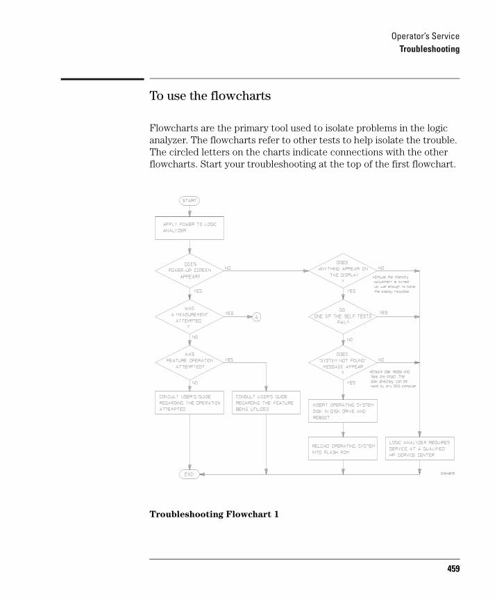
Operator’s ServiceTroubleshooting
To use the flowcharts
Flowcharts are the primary tool used to isolate problems in the logic analyzer. The flowcharts refer to other tests to help isolate the trouble. The circled letters on the charts indicate connections with the other flowcharts. Start your troubleshooting at the top of the first flowchart.
Troubleshooting Flowchart 1
459
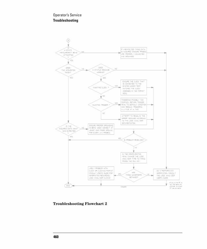
Operator’s ServiceTroubleshooting
Troubleshooting Flowchart 2
460
Operator’s ServiceTroubleshooting
To check the power-up tests
The logic analyzer automatically performs power-up tests when you apply power to the instrument. The revision number of the operating system shows in the upper-right corner of the screen during these power-up tests. As each test completes, either "passed" or "failed" prints on the screen in front of the name of each test.
1 Disconnect all inputs, then insert a formatted disk into the flexible disk drive.
2 Let the analyzer warm up for a few minutes, then cycle power by turning off then turning on the power switch.
If the analyzer is not warmed up, the power-up test screen will complete before you can view the screen.
3 As the tests complete, check if they pass or fail.
The Flexible Disk Test reports No Disk if a disk is not in the disk drive.
Performing Power-Up Self-Tests
passed ROM textpassed RAM testpassed Interrupt testpassed Display testpassed PS2 Controller Testpassed Hard Disk TestNo Disk Flexible Disk Test
461
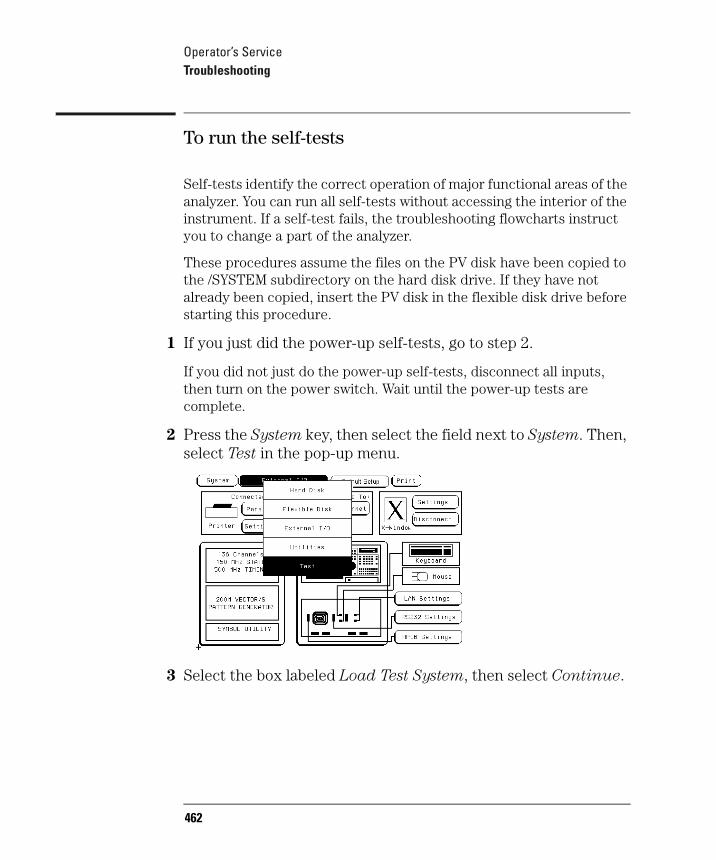
Operator’s ServiceTroubleshooting
To run the self-tests
Self-tests identify the correct operation of major functional areas of the analyzer. You can run all self-tests without accessing the interior of the instrument. If a self-test fails, the troubleshooting flowcharts instruct you to change a part of the analyzer.
These procedures assume the files on the PV disk have been copied to the /SYSTEM subdirectory on the hard disk drive. If they have not already been copied, insert the PV disk in the flexible disk drive before starting this procedure.
1 If you just did the power-up self-tests, go to step 2.
If you did not just do the power-up self-tests, disconnect all inputs, then turn on the power switch. Wait until the power-up tests are complete.
2 Press the System key, then select the field next to System. Then, select Test in the pop-up menu.
3 Select the box labeled Load Test System, then select Continue.
462
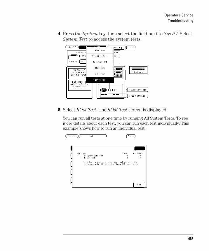
Operator’s ServiceTroubleshooting
4 Press the System key, then select the field next to Sys PV. Select System Test to access the system tests.
5 Select ROM Test. The ROM Test screen is displayed.
You can run all tests at one time by running All System Tests. To see more details about each test, you can run each test individually. This example shows how to run an individual test.
463
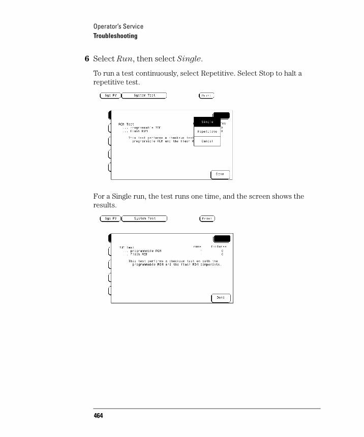
Operator’s ServiceTroubleshooting
6 Select Run, then select Single.
To run a test continuously, select Repetitive. Select Stop to halt a repetitive test.
For a Single run, the test runs one time, and the screen shows the results.
464
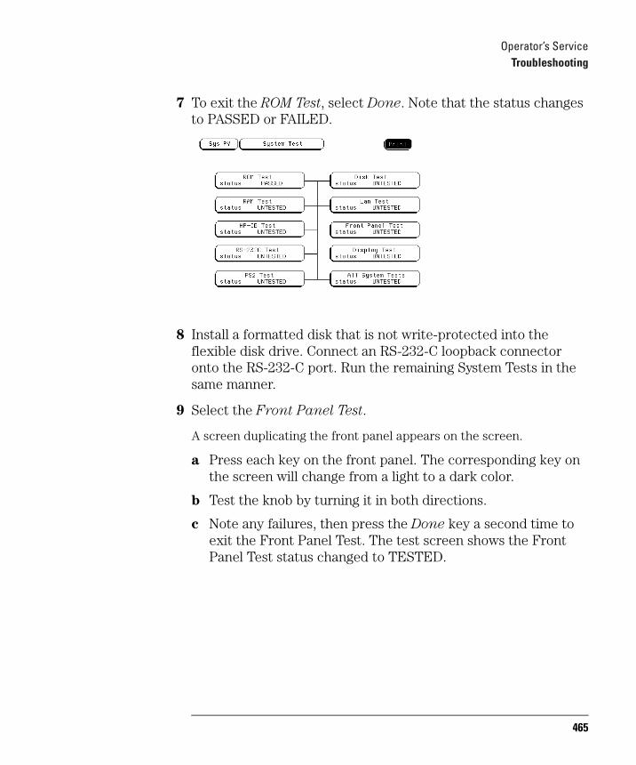
Operator’s ServiceTroubleshooting
7 To exit the ROM Test, select Done. Note that the status changes to PASSED or FAILED.
8 Install a formatted disk that is not write-protected into the flexible disk drive. Connect an RS-232-C loopback connector onto the RS-232-C port. Run the remaining System Tests in the same manner.
9 Select the Front Panel Test.
A screen duplicating the front panel appears on the screen.
a Press each key on the front panel. The corresponding key on the screen will change from a light to a dark color.
b Test the knob by turning it in both directions.
c Note any failures, then press the Done key a second time to exit the Front Panel Test. The test screen shows the Front Panel Test status changed to TESTED.
465

Operator’s ServiceTroubleshooting
10 Select the Display Test.
A white grid pattern is displayed. These display screens can be used to adjust the display.
a Select Continue and the screen changes to full bright.
b Select Continue and the screen changes to half bright.
c Select Continue and the test screen shows the Display Test status changed to TESTED.
11 Select Sys PV, then select Analy PV in the pop-up menu. Select Chip 2 Tests.
You can run all the analyzer tests at one time by selecting All Analyzer Tests. To see more details about each test, you can run each test individually. This example shows how to run Chip 2 Tests. Chip 3, 4, and 5 Tests operate the same as Chip 2 Tests.
466
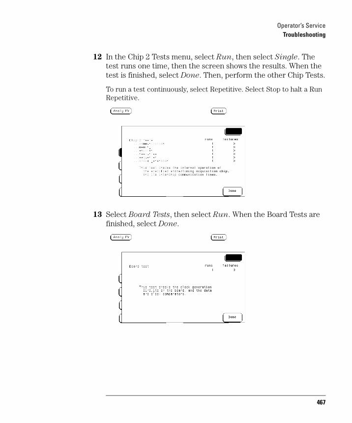
Operator’s ServiceTroubleshooting
12 In the Chip 2 Tests menu, select Run, then select Single. The test runs one time, then the screen shows the results. When the test is finished, select Done. Then, perform the other Chip Tests.
To run a test continuously, select Repetitive. Select Stop to halt a Run Repetitive.
13 Select Board Tests, then select Run. When the Board Tests are finished, select Done.
467

Operator’s ServiceTroubleshooting
14 Select Data Input Inspection. All lines should show activity. Select Done to exit the Data Input Inspection.
15 If you do not have a 1670G-series logic analyzer with the oscilloscope option, exit the tests by pressing the System key. Select the field to the right of the Sys PV field. Select the Exit
Test System.
16 If you have a 1670G-series logic analyzer with the oscilloscope option, select Analy PV, then select Scope PV in the pop up menu. Select Functional Tests.
468
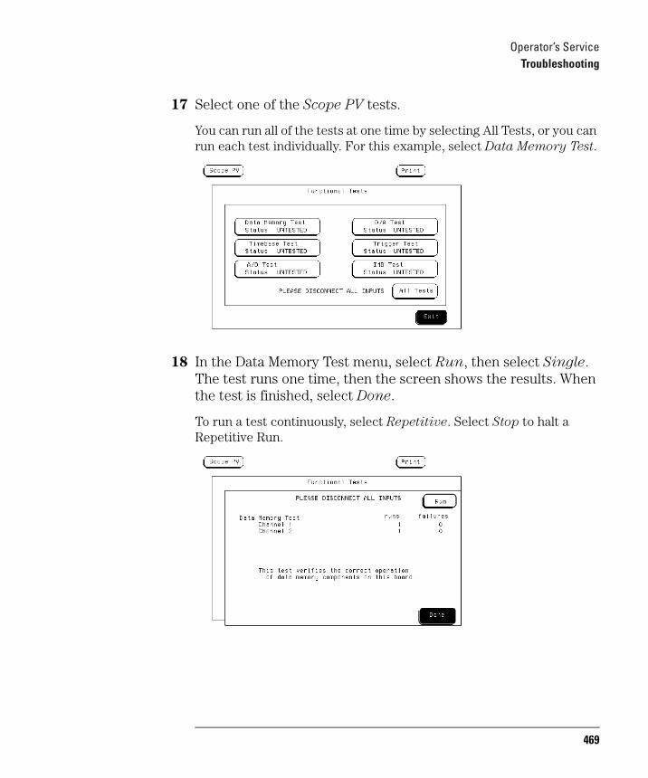
Operator’s ServiceTroubleshooting
17 Select one of the Scope PV tests.
You can run all of the tests at one time by selecting All Tests, or you can run each test individually. For this example, select Data Memory Test.
18 In the Data Memory Test menu, select Run, then select Single. The test runs one time, then the screen shows the results. When the test is finished, select Done.
To run a test continuously, select Repetitive. Select Stop to halt a Repetitive Run.
469
Operator’s ServiceTroubleshooting
19 To exit the tests, press the System key. Select the field to the right of the Sys PV field.
20 Select the Exit Test System.
If you are performing the self-tests as part of the troubleshooting flowchart, return to the flowchart.
470
Operator’s ServiceTroubleshooting
To test the auxiliary power
The +5 V auxiliary power is protected by a current overload protection device. If the current on pins 1 and 39 exceed 0.33 amps, the circuit will open. When the short is removed, the circuit will reset in approximately 1 minute. There should be +5 V after the 1 minute reset time.
Equipment Required
Equipment Critical Specifications RecommendedAgilent Model/Part
Digital Multimeter 0.1 mV resolution, 3478Abetter than 0.005% accuracy
• Using the multimeter, verify the +5 V on pins 1 and 39 of the probe cables.
471

Operator’s ServiceTroubleshooting
472
Section 2
LAN
473

474

15
Introducing the LAN Interface
475

Introducing the LAN InterfaceIntroducing the LAN Interface
Introducing the LAN InterfaceThe Agilent Technologies Logic Analyzer LAN interface lets you connect your logic analyzer to an Ethernet network that uses TCP/IP. With the LAN Interface, you can:
• Set up and run measurements using the logic analyzer's XWindow interface.
• Copy measurement data from the logic analyzer to your computer using File Transfer Protocol program (ftp) or Network File System (NFS).
• Save and restore configurations.
• Program the logic analyzer.
Requirements
In order to use your 1670G logic analyzer on the LAN, you need the following equipment and software:
• Ethernet local area network using TCP/IP protocol.
• If you are using a PC, NFS program or ftp program.
• If you want to use the logic analyzer's XWindow interface, Xserver program running on your computer.
Characteristics
Physical Connection.
• RJ-45 connector for direct connection to 10Base-T ("ethertwist") networks
• BNC connector for direct connection to 10Base2 ("thinlan") networks
476
Introducing the LAN InterfaceIntroducing the LAN Interface
Supported Protocols.
• Transmission Control Protocol/Internet Protocol (TCP/IP)
• Network File System (NFS)
• File Transfer Protocol (ftp)
• X Window System Version 11, release 5 (X11R5)
• Simple Network Management Protocol (SNMP)
477
Introducing the LAN InterfaceIntroducing the LAN Interface
LAN section overview
The chapters in the LAN section of this User’s Guide shows you how to connect, use, and troubleshoot your logic analyzer via a Local Area Network (LAN) connection. The following is a brief description of each chapter.
Connecting and Configuring. Provides information about connecting the logic analyzer to the network. To effectively use this chapter, you should be familiar with your network setup and operation.
Accessing the Logic Analyzer File System. Shows you how to access the logic analyzer’s file system. This is a prerequisite for some of the other things you can do with a logic inlayer on the network.
Using the X Window Interface. Shows you how to display the analyzer interface on an X Window server, and describes the basics of using the interface.
Retrieving and Restoring Data. Shows you how to retrieve measurement data, screen images, and status information from your logic analyzer on the LAN, and how to copy and restore configurations.
Programming the Logic analyzer. Shows you methods for programming the logic analyzer via the network connection.
Concepts. Contains additional information on the logic analyzer’s directory structure and dynamic files.
Troubleshooting. Describes what to do if you have a problem using the logic analyzer on your network.
478
16
Connecting and Configuring the LAN
479

Connecting and Configuring the LANConnecting and Configuring the LAN
Connecting and Configuring the LANIn order to use your logic analyzer's network capabilities, you need to connect it to your network and configure the logic analyzer.
The following chart shows an overview of the process.
Connect
Configure
Ping
Mount
Connect the RJ-45 or BNC connector from your network, then turn on the logic analyzer.
Setup the configuration menus.
Verify connectivity with the ping utility.Ping OK?
Mount the logic analyzer. Mount OK?
Ready to use.
Yes
Yes
Go to page 536, “Troubleshooting the LAN.”
Go to page 536, “Troubleshooting the LAN.”
No
No
480
Connecting and Configuring the LANConnecting and Configuring the LAN
To connect to your network
1 Turn off the logic analyzer.
2 Connect the analyzer to your network using an RJ-45 or BNC connector.
Ethertwist and thinlan are the two most common types of LAN network connection. Ethertwist uses unshielded twisted pair and an RJ-45 connector, and resembles a standard modular phone line. Thinlan uses coaxial cable. If you are unsure what your network uses for its physical connection, contact your local network administrator.
The logic analyzer LAN ports are on the back panel. The RJ-45 connector goes in the port labeled "LAN-TP" and the BNC attaches to the port labeled "LAN-BNC".
3 Turn on the logic analyzer.
481
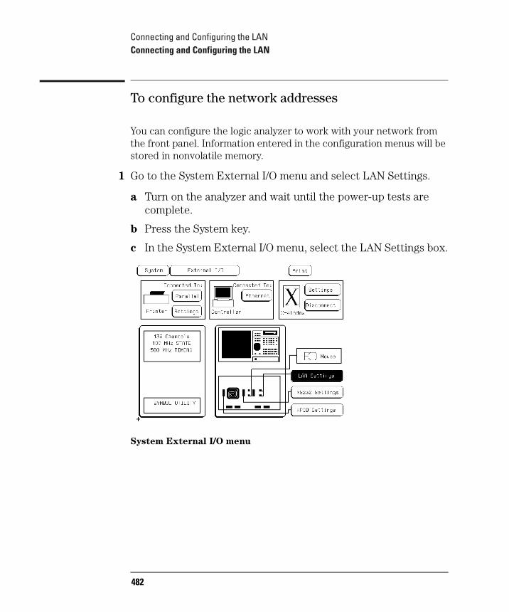
Connecting and Configuring the LANConnecting and Configuring the LAN
To configure the network addresses
You can configure the logic analyzer to work with your network from the front panel. Information entered in the configuration menus will be stored in nonvolatile memory.
1 Go to the System External I/O menu and select LAN Settings.
a Turn on the analyzer and wait until the power-up tests are complete.
b Press the System key.
c In the System External I/O menu, select the LAN Settings box.
System External I/O menu
482
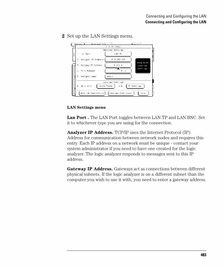
Connecting and Configuring the LANConnecting and Configuring the LAN
2 Set up the LAN Settings menu.
LAN Settings menu
Lan Port . The LAN Port toggles between LAN TP and LAN BNC. Set it to whichever type you are using for the connection.
Analyzer IP Address. TCP/IP uses the Internet Protocol (IP) Address for communication between network nodes and requires this entry. Each IP address on a network must be unique - contact your system administrator if you need to have one created for the logic analyzer. The logic analyzer responds to messages sent to this IP address.
Gateway IP Address. Gateways act as connections between different physical subnets. If the logic analyzer is on a different subnet than the computer you wish to use it with, you need to enter a gateway address.
483

Connecting and Configuring the LANConnecting and Configuring the LAN
File Timeout. This is not the same as the network timeout, which is set on the computer. The logic analyzer file timeout is how long the analyzer keeps a file in the active portion of memory. For slow network connections, a large file timeout decreases the total time for a file transfer. Too high a file timeout for a fast network connection can actually slow file transfers because too much is in active memory. A good guideline for file timeout is 150% of the average time it takes for packets to go from source to destination.
Analyzer Name. The Analyzer Name is for user reference only. It appears in the status files of the logic analyzer, and in the X Window display. It is not the same as the IP name.
3 If necessary, add the logic analyzer to your local network configuration.
If you are doing a point-to-point connection, this step is unnecessary because the computer and the logic analyzer only communicate with each other.
For UNIX networks and PC networks based on a UNIX model, the network software requires an entry for the logic analyzer before another computer can talk to it. These entries are usually kept in a file named /etc/hosts. The /etc/hosts file also associates an alias with the IP address so that you can use a meaningful name rather than the IP address.
Other styles of PC networks have different conventions. Consult your LAN documentation or your local system administrator to see if you need to do anything else.
484
Connecting and Configuring the LANConnecting and Configuring the LAN
To verify connectivity with the ping utility
Use the ping utility to verify that the logic analyzer is on your network.
Refer to your network documentation for the exact syntax.
• UNIXping [IP address|symbolic name]
• MS-DOSping [IP address|symbolic name]
• MS WindowsFor a Windows environment, select the ping icon in your network menu. Refer to your network documentation for more information about using the ping utility.
485
Connecting and Configuring the LANConnecting and Configuring the LAN
To mount the logic analyzer
NOTE: Before MountingYou need to wait at least 15 seconds after the Analyzer Configuration menu is displayed before attempting to mount. If you try to mount too soon, you will receive an error message.
You can mount the logic analyzer on your network for two different levels of use, control or data. The logic analyzer accommodates one control user and multiple data users. Control allows users to read and write files to and from the analyzer, while data allows users to only read files from the file system. Data users can also write files to the disk drives of the logic analyzer.
If you have trouble, refer to chapter 7, "Troubleshooting."
For the exact syntax of the mount command for mount, refer to your network documentation.
NOTE: Mounting and UnmountingYou must unmount the logic analyzer before turning it off. After unmounting, you can mount the analyzer 15 seconds after the Analyzer Configuration menu is displayed when powering up the instrument. You can write a network script that executes an unmount and mount procedure.
486

Connecting and Configuring the LANConnecting and Configuring the LAN
• UNIX
For UNIX, use your network's command for an NFS mount.
For example:
mount [analyzer name:]/[control|data][mount point]
Some UNIX workstations will not accept a straight IP address. You must add an aliased name for the logic analyzer to the host file, then use that name in your mount command.
Refer to your network documentation for more information.
• MS-DOS
For a PC using MS-DOS and running PC-NFS, use a form of the net use command.
For example, PC-NFS uses:
net use [drive specifier][IP address or a named alias]\ [control|data]
Refer to your PC-based NFS documentation for more information.
• MS Windows
For an MS Windows environment, refer to your Windows-based NFS documentation and File Manager documentation for mounting instructions.
487

Connecting and Configuring the LANConnecting and Configuring the LAN
488

17
Accessing the Logic Analyzer File System Using the LAN
489

Accessing the Logic Analyzer File System Using the LANAccessing the Logic Analyzer File System Using the LAN
Accessing the Logic Analyzer File System Using the LANThis chapter shows you how to:
• Mount the file system via NFS.
• Access the file system via ftp.
NOTE: This chapter assumes that the logic analyzer is physically connected to your local area network. If it is not connected, refer to Chapter 1 for information on how to connect the system.
Control User vs. Data User
You can access the logic analyzer file system as either the control user or a data user.
Control User
• The control user can send programming commands.
• The control user has read and write access to the file system.
• There can only be one control user at any time.
Data User
• The data user cannot send programming commands.
• The data user has read access to the entire file system, but can only write to \system\disk\hard and \system\disk\flexible directories (the logic analyzer disk drives).
• Multiple data users can access the logic analyzer simultaneously.
Password and File Protection
There is no password protection built into the logic analyzer. This means that files are not protected against either deletion or being written over.
490

Accessing the Logic Analyzer File System Using the LANAccessing the Logic Analyzer File System Using the LAN
To mount the file system via NFS
NOTE: The logic analyzer must be on and completely booted up before you can mount the file system. Once power is applied and the Analyzer Configuration menu is displayed, allow an additional 15 seconds before attempting to mount the system.
NOTE: Be sure to unmount the logic analyzer's file system before turning off the logic analyzer. If you don't do this, you may get a "stale NFS file handle" error message the next time you try to mount. If you get this message, unmount the file system and try mounting again.
From Computers Running the UNIX Operating System
The syntax of the mount command is typically
mount [symbolic name|IP address]:/[control|data] /[directory name]
The symbolic name is the host name of the logic analyzer as set up by your system administrator. Typically, this name is found in the /etc/hosts file on your computer or returned by a name server. It is equivalent to the logic analyzer's IP (Internet Protocol) address.
The control or data option specifies the type of access you want.
The directory name is the name of an empty directory in your computer's file system to which the logic analyzer's file system will be mounted.
See the example on the next page.
491
Accessing the Logic Analyzer File System Using the LANAccessing the Logic Analyzer File System Using the LAN
Example Mounting the logic analyzer on a UNIX computer
To mount the analyzer named "1670G_1" as the control user to a directory on your computer named /logic, enter the following command at the UNIX command line:
mount 1670G_1:/control /logic
After you have entered this command, you will be able to see the logic analyzer's file system under the /logic directory on your computer.
To unmount:
umount /logic
492

Accessing the Logic Analyzer File System Using the LANAccessing the Logic Analyzer File System Using the LAN
From Computers Running the MS-DOS Operating System
NOTE: To use the logic analyzer interface in an MS-DOS environment, you need to install a program on your PC that allows you to use NFS protocol. One such program is PC-NFS by SunSoft Inc.
To mount the logic analyzer file system from a PC running MS-DOS, you must create a logical drive that points to it. A typical MS-DOS command to do this would look like one of these two examples:
net use [drive name] [host name|IP address]:/[control|data]
net use [drive name] \\[host name|IP address]\[control|data]
The choice of drive name is up to you.
The host name of the logic analyzer is set up by your system administrator. Typically, this name is found in the hosts file on your computer or returned by a name server. It is equivalent to the logic analyzer's IP (Internet Protocol) address.
The control or data option specifies the type of access you want.
Example Mounting the logic analyzer with MS-DOS
To mount, as the control user, the logic analyzer whose IP address is "15.6.254.150" to the logical drive "L:", enter the following command at the MS-DOS prompt. In this example, the PC-NFS application is used.
net use L: 15.6.254.150:/control
After you have entered this command, you will be able to see the analyzer's file system under the "L:" logical drive on your computer.
To unmount:
net use L: /d
493
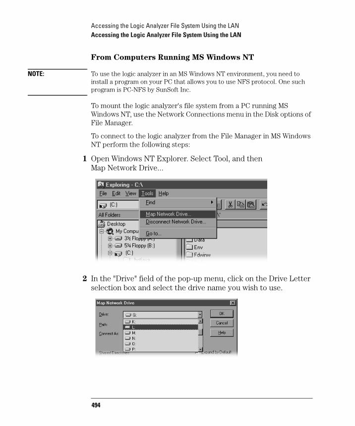
Accessing the Logic Analyzer File System Using the LANAccessing the Logic Analyzer File System Using the LAN
From Computers Running MS Windows NT
NOTE: To use the logic analyzer in an MS Windows NT environment, you need to install a program on your PC that allows you to use NFS protocol. One such program is PC-NFS by SunSoft Inc.
To mount the logic analyzer's file system from a PC running MS Windows NT, use the Network Connections menu in the Disk options of File Manager.
To connect to the logic analyzer from the File Manager in MS Windows NT perform the following steps:
1 Open Windows NT Explorer. Select Tool, and then Map Network Drive...
2 In the "Drive" field of the pop-up menu, click on the Drive Letter selection box and select the drive name you wish to use.
494

Accessing the Logic Analyzer File System Using the LANAccessing the Logic Analyzer File System Using the LAN
3 In the Path field, type the name of the server that the logic analyzer system is mounted on, followed by the analyzer's name or IP address. At the end of the path, specify which kind of connection you would like to establish, either "control" or "data".
495
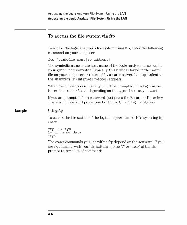
Accessing the Logic Analyzer File System Using the LANAccessing the Logic Analyzer File System Using the LAN
To access the file system via ftp
To access the logic analyzer's file system using ftp, enter the following command on your computer:
ftp [symbolic name|IP address]
The symbolic name is the host name of the logic analyzer as set up by your system administrator. Typically, this name is found in the hosts file on your computer or returned by a name server. It is equivalent to the analyzer's IP (Internet Protocol) address.
When the connection is made, you will be prompted for a login name. Enter "control" or "data" depending on the type of access you want.
If you are prompted for a password, just press the Return or Enter key. There is no password protection built into Agilent logic analyzers.
Example Using ftp
To access the file system of the logic analyzer named 1670sys using ftp enter:
ftp 1670syslogin name: dataftp>
The exact commands you use within ftp depend on the software. If you are not familiar with your ftp software, type "?" or "help" at the ftp prompt to see a list of commands.
496

18
Using the LAN’s X Window Interface
497
Using the LAN’s X Window InterfaceUsing the LAN’s X Window Interface
Using the LAN’s X Window InterfaceThis chapter shows you how to:
• Start the interface.
• Close the interface.
• Load the custom fonts.
Using the Mouse and Keyboard
Once you have started the XWindow interface and are displaying it on your computer running the Xserver, you can use your computer's keyboard and mouse to control the logic analyzer interface in the same way you use the logic analyzer's keyboard and mouse. Refer to your logic analyzer's User's Guide for a complete description of keyboard and mouse operation.
Duplicating Front-Panel Knob Control
To duplicate turning the knob, hold down the right mouse button, and move the mouse up or to the right for clockwise knob movement; move the mouse down or to the left for counter-clockwise knob movement.
You can also use the keyboard's Shift-up or -right arrow keys to duplicate clockwise knob movement. Use the Shift-down or -left arrow keys to duplicate counter-clockwise knob movement.
498
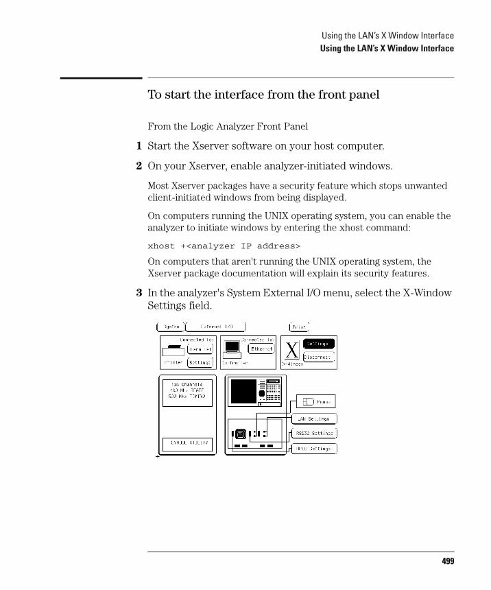
Using the LAN’s X Window InterfaceUsing the LAN’s X Window Interface
To start the interface from the front panel
From the Logic Analyzer Front Panel
1 Start the Xserver software on your host computer.
2 On your Xserver, enable analyzer-initiated windows.
Most Xserver packages have a security feature which stops unwanted client-initiated windows from being displayed.
On computers running the UNIX operating system, you can enable the analyzer to initiate windows by entering the xhost command:
xhost +<analyzer IP address>
On computers that aren't running the UNIX operating system, the Xserver package documentation will explain its security features.
3 In the analyzer's System External I/O menu, select the X-Window Settings field.
499
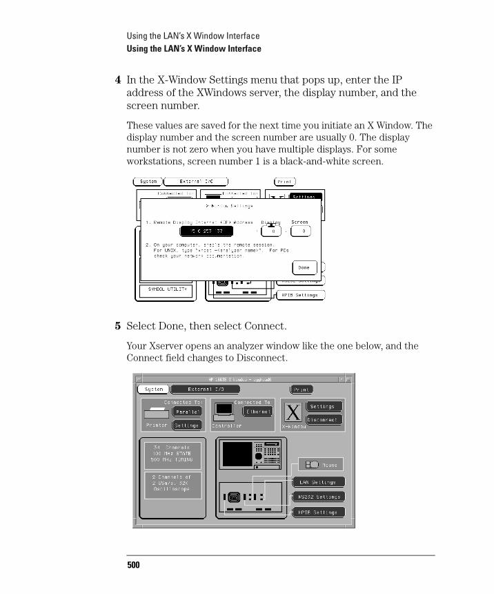
Using the LAN’s X Window InterfaceUsing the LAN’s X Window Interface
4 In the X-Window Settings menu that pops up, enter the IP address of the XWindows server, the display number, and the screen number.
These values are saved for the next time you initiate an X Window. The display number and the screen number are usually 0. The display number is not zero when you have multiple displays. For some workstations, screen number 1 is a black-and-white screen.
5 Select Done, then select Connect.
Your Xserver opens an analyzer window like the one below, and the Connect field changes to Disconnect.
500
Using the LAN’s X Window InterfaceUsing the LAN’s X Window Interface
To start the interface from the computer
1 On your Xserver, enable analyzer-initiated windows.
Most Xserver packages have a security feature which stops unwanted client-initiated windows from being displayed.
On computers running the UNIX operating system, you can enable analyzer-initiated windows by entering the xhost command:
xhost +<analyzer IP address>
On computers that aren't running the UNIX operating system, the Xserver package documentation will explain its security features.
2 Send the XWIN ON programming command to the logic analyzer.
The syntax of the XWIN ON command is:
xwin on,"<Xserver IP address>:<display>.<screen>"
The IP (Internet Protocol) address is the address of the XWindows server.
There are several methods for sending the XWIN ON command. The easiest is using psuedo-telnet, but it can also be done using ftp or writing to the NFS-mounted logic analyzer. See the following examples.
Example NFS method using a UNIX computer
To enable windows to be initiated from the logic analyzer named lp1670G, enter the following command on the computer running the Xserver:
xhost +lp1670G
If you have NFS mounted the analyzer's file system to a directory named /logic on your computer whose IP address is 15.6.253.146 (and is running the Xserver), enter the following command to start the XWindow interface:
echo "xwin on,'15.6.253.146:0.0'" > /logic/system/program
501
Using the LAN’s X Window InterfaceUsing the LAN’s X Window Interface
Example Pseudo telnet method using a UNIX computer
To enable windows to be initiated from the logic analyzer named lp1670G, enter the following command on the computer running the Xserver :
xhost +lp1670G
To connect to the command parser socket of the logic analyzer named lp1670G, enter:
telnet lp1670G 5025
NOTE: Agilent Technologies logic analyzers are not telnet servers. The UNIX command telnet is used to make a connection to the analyzer command parser, which uses socket number 5025. A telnet server would normally not need to have the socket specified.
To start the XWindow interface on the computer whose IP address is 15.6.253.146 (and is running the Xserver) enter:
xwin on,"15.6.253.146:0.0"
If you are not planning on sending more commands to the logic analyzer, close the telnet connection by typing the escape character, and then "quit" when the telnet prompt appears. The escape character is often Control-]; your telnet program should tell you when it opens the connection.
502

Using the LAN’s X Window InterfaceUsing the LAN’s X Window Interface
Example ftp method using a UNIX computer
File transfer protocol (ftp) can be used to start the X Window interface from either a UNIX computer or a PC. The logic analyzer is named lp1670G in this example. You will need to start the X server software on a PC and may need to enable the analyzer-initiated window. On a UNIX computer, you will need to enable the window initiated by the logic analyzer by entering the following command:
xhost +lp1670G
Next, create a text file with the following contents (where 15.6.253.146 is the IP address of the X server with display 0 and screen 0 selected):
xwin on,'15.6.253.146:0.0'<cr>
Log in as “control”.
name: control
We will name the text file "startx" for this example. At an ftp command prompt, copy this file from your local directory to a virtual file called "program" in the logic analyzer \system directory as follows:
ftp> cd systemftp> put startx program
This causes the contents of the file to be executed by the logic analyzer command parser and a window to appear on the X server.
503
Using the LAN’s X Window InterfaceUsing the LAN’s X Window Interface
To close the interface
From the XWindow Interface or Front Panel
1 Go to the System External I/O menu.
2 Select the Disconnect field.
The interface on your Xserver closes, and the Disconnect field changes to Connect.
From a Remote Computer
• Send the XWIN OFF programming command to the logic analyzer.
NOTE: Note that simply closing the window that the interface is running in may leave the logic analyzer hung up.
Example ftp method
To end the session using ftp, create a second text file with the following contents:
xwin off<cr>
The second text file is named "stopx". At an ftp command prompt, copy this file from your local directory to a virtual file called "program" in the logic analyzer \system directory as follows:
ftp> cd systemftp> put stopx program
504
Using the LAN’s X Window InterfaceUsing the LAN’s X Window Interface
To load the custom fonts
1 From the computer running your Xserver software, access the logic analyzer's file system.
Refer to the "Accessing the Logic Analyzer File System" chapter.
2 Copy the SM165.BDF and LG165.BDF files from the analyzer's \system\disk\hard\system directory to a directory on your computer.
3 Set up the Xserver so that it can read these fonts.
Refer to your XWindows server documentation for instructions on loading and using custom fonts. Generally, the steps you will take are:
a Compile the .BDF files into the proper format.
b Build the font directory (FONTS.DIR) file.
c If the font directory is not in the current font path, add the new directory to the font path.
The custom fonts make the analyzer's XWindow interface look identical to the instrument's display. If the custom fonts are not loaded, you will see odd characters in place of arrow symbols and may see out-of-bounds text in the XWindow image.
505

Using the LAN’s X Window InterfaceUsing the LAN’s X Window Interface
Example Loading the fonts using ftp and UNIX
Suppose you have a UNIX computer running your Xserver software. Go to the directory where you want to install the custom fonts. As the data user, ftp to the analyzer and copy SM165.BDF and LG165.BDF from the \system\disk\hard\system directory to your computer.
ftp lp1670G220 Agilent 1670G V01.00 FUSION FTP server (Version 3.3) ready.Name (lp1670G:guest): data230 User DATA logged in.ftp> cd /system/disk/hard/system200 Remote Directory changed to "/system/disk/hard/system".ftp> get lg165.bdf200 PORT command ok.150 Opening data connection for lg165.bdf (15.6.253.146,1121) (20494 bytes).226 Transfer complete.23338 bytes received in 0.69 seconds (32.82 Kbytes/s)ftp> get sm165.bdf200 PORT command ok.150 Opening data connection for sm165.bdf (15.6.253.146,1122) (19595 bytes).226 Transfer complete.22311 bytes received in 0.32 seconds (68.04 Kbytes/s)ftp> quit
To create a fonts.dir file in the current directory:
mkfontdir
To prepend the current directory to the font path:
xset +fp /users/guest/165fonts
To reset the font path to its current value:
xset fp rehash
506

Using the LAN’s X Window InterfaceUsing the LAN’s X Window Interface
Close the analyzer's XWindow interface and re-start it. You should now see the same fonts that are used on the logic analyzer's front panel display.
The xset commands must either be repeated each time X is restarted or the fonts must be installed in the default X11 font directory, typically found in /usr/lib/X11/fonts/misc. This directory is usually protected, so your system administrator may have to perform the installation.
507

Using the LAN’s X Window InterfaceUsing the LAN’s X Window Interface
Additional Information
Color
The X Window that appears on your X Server is in color. If another application such as a Web browser is using many colors, the X Window may be unreadable when it appears. If so, close the X Window, free some colors by closing another application, and restart the X Window. Computers that are configured to support only 16 colors will substitute for some default colors.
Window Dimensions and Content
The dimensions of the logic analyzer window are set at 640 x 480 pixels and the X Window dimensions are 576 x 378. The actual size of the window will vary with the physical and pixel dimensions of your computer display. Re-sizing the window will not add more content.
508
19
Retrieving and Restoring Data Using the LAN
509
Retrieving and Restoring Data Using the LANRetrieving and Restoring Data Using the LAN
Retrieving and Restoring Data Using the LANThis chapter shows you how to:
• Copy ASCII measurement data.
• Copy raw measurement data.
• Restore raw measurement data.
• Copy screen images from \system\graphics.
• Copy status information from \status.
• Copy configurations from the logic analyzer.
• Restore configurations to the logic analyzer.
Measurement data is available in binary format and also in ASCII format. Screen images are available in TIFF, PCX, and Encapsulated PostScript formats.
510
Retrieving and Restoring Data Using the LANRetrieving and Restoring Data Using the LAN
To copy ASCII measurement data
1 Set up the measurement you want to make, and run the analyzer to acquire data.
For more information on setting up measurements, see the Logic Analyzer section of this book.
2 Access the logic analyzer's file system.
Refer to the chapter "Accessing the Logic Analyzer File System".
You can do this from the XWindow interface, your computer using NFS or ftp, from the front panel, or by programming the logic analyzer.
3 Copy the measurement data from the \slot_a\data.asc subdirectory.
In the analyzer's file system, ASCII data files are located in \slot_a\data.asc\analyzer name\label name.txt.
There is an ASCII data file corresponding to each label name you have created in the measurement module. The data files for each label are overwritten by the analyzer each time new data is acquired.
NOTE: 1670G-Series with the oscilloscope option onlyOscilloscope data is under \slot_b\data.asc. There is no subdirectory matching analyzer name but there are files for both oscilloscope channels.
511
Retrieving and Restoring Data Using the LANRetrieving and Restoring Data Using the LAN
To copy raw measurement data
1 Set up the measurement you want to make, and run the analyzer to acquire data.
For more information on setting up measurements, see the Logic Analyzer section of this book. You can set up and run the measurement from the analyzer's XWindow interface or front panel, or by programming the analyzer.
2 Access the logic analyzer's file system.
Refer to the chapter "Accessing the Logic Analyzer File System".
3 Copy the data.raw file from the \slot_a directory for analyzer data, or \slot_b directory for oscilloscope data.
Raw measurement data files are binary format files that can be transferred to your computer and then reloaded into the logic analyzer later. Because they are binary files, if you are using ftp to upload or download them, set the type to binary by typing "bin" at the ftp prompt.
The data.raw file is overwritten each time new data is acquired.
512
Retrieving and Restoring Data Using the LANRetrieving and Restoring Data Using the LAN
To restore raw measurement data
1 Access the analyzer's file system as the control user.
Refer to the chapter "Accessing the Logic Analyzer File System".
2 Copy the data.raw file to the appropriate \slot_x directory.
For analyzer data, this would be the \slot_a directory. For oscilloscope data, it would be \slot_b. If you copy the raw data to a different directory than you originally got it from, the logic analyzer won't know how to interpret it.
Raw measurement data files are binary format files. Because they are binary files, if you are using ftp to upload or download them, set the type to binary by typing "bin" at the ftp prompt.
The data.raw file is overwritten each time new data is acquired.
513
Retrieving and Restoring Data Using the LANRetrieving and Restoring Data Using the LAN
To copy screen images from \system\graphics
1 Access the logic analyzer's file system.
Refer to the chapter "Accessing the Logic Analyzer File System".
2 Set up the screen you want to copy.
3 Copy the screen image file from the \system\graphics directory.
The \system\graphics directory contains the following files:
• screen.tif - a color TIFF file, in TIFF version 5.0 format.
• screenbw.tif - a color TIFF file in TIFF version 5.0 format.
• screen.pcx - a color PCX file.
• screenbw.epi - a black-and-white Encapsulated PostScript file in EPS version 3.0 format.
NOTE: These graphics files contain the current display on the logic analyzer screen. The contents of the files change whenever you change the display. When you copy one of the graphics files, the display will freeze for a few moments to make a copy of the current display.
514

Retrieving and Restoring Data Using the LANRetrieving and Restoring Data Using the LAN
To copy status information from \status
1 Access the logic analyzer's file system.
Refer to the chapter "Accessing the Logic Analyzer File System".
2 Copy the appropriate file from the \status directory.
The \status directory contains the following ASCII files:
• system.txt - shows whether the analyzer is running or stopped. It also includes information about the Group Run and the relative trigger times of each module if applicable.
• frame.txt - shows what is mapped to each slot and the operating system version.
• mount.txt - lists all connections to the logic analyzer. The connection information includes the IP address and user type. This information is also available in the External I/O LAN Settings menu, under Show LAN Connections.
Example An example system.txt file:
Analyzer name: LP LAN Analyzer
Execution Status: slot_a - stopped
515
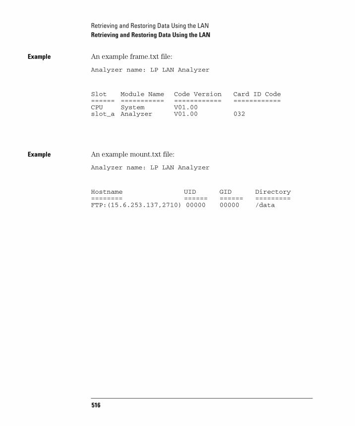
Retrieving and Restoring Data Using the LANRetrieving and Restoring Data Using the LAN
Example An example frame.txt file:
Analyzer name: LP LAN Analyzer
Slot Module Name Code Version Card ID Code====== =========== ============ ============CPU System V01.00 slot_a Analyzer V01.00 032
Example An example mount.txt file:
Analyzer name: LP LAN Analyzer
Hostname UID GID Directory ======== ====== ====== =========FTP:(15.6.253.137,2710) 00000 00000 /data
516
Retrieving and Restoring Data Using the LANRetrieving and Restoring Data Using the LAN
To copy configurations from setup.raw
1 Set up the configuration.
You can do this from the XWindow interface or from the front panel.
2 Access the logic analyzer's file system.
Refer to the chapter "Accessing the Logic Analyzer File System".
3 Copy the setup.raw file from the appropriate directory.
For system configurations, the appropriate directory is \system . For analyzer configurations, the appropriate directory is \slot_a . For oscilloscope configurations, the appropriate directory is \slot_b .
Raw configuration files are binary format files that can be transferred to your computer and then reloaded into the logic analyzer later. Raw configuration files are not transferable between logic analyzer models.
The setup.raw file is overwritten whenever you change the configuration.
Dynamic Configuration Files
Configuration files are dynamic files. When you look at the logic analyzer file system, dynamic files show a file size of 1 or 0. 0 means there isn't anything available and 1 means there is. When you request the dynamic file, the logic analyzer creates it. While the analyzer is creating the file, it will not respond to other requests. Because the analyzer does not know the file size until it is created, some NFS systems have trouble copying dynamic files. If the cp command does not appear to work, try using dd.
517
Retrieving and Restoring Data Using the LANRetrieving and Restoring Data Using the LAN
To restore configurations
1 Access the logic analyzer's file system as the control user.
Refer to the chapter "Accessing the Logic Analyzer File System".
2 Copy the setup.raw file to the appropriate directory.
For system configurations, this would be the \system directory. For analyzer configurations, this would be the \slot_a directory. For oscilloscope configurations, it would be the \slot_b directory. If you copy a configuration file to a different directory than it came from, the analyzer will not know how to interpret it.
Example Restoring an analyzer configuration
Suppose you want to load a configuration file called "486_bus" from your local computer into the logic analyzer's analyzer. The analyzer is always in slot A. The logic analyzer is mounted on your network as disk drive L:.
To load the configuration file, at the MS-DOS prompt enter:
copy 486_bus L:\slot_a\setup.raw
If your computer is running the UNIX operating system, you might use the cp command. In an MSWindows environment, you can use File Manager.
518
20
Programming the Logic Analyzer Using the LAN
519
Programming the Logic Analyzer Using the LANProgramming the Logic Analyzer Using the LAN
Programming the Logic Analyzer Using the LANYou can program the logic analyzer over the Local Area Network (LAN) by sending commands to the \system\program file or by sending commands to the command parser socket.
This chapter shows you how to:
• Set up for Ethernet programming.
• Enter commands directly using telnet.
• Write programs that open the command parser socket.
The logic analyzer does not provide real-time programming control. Due to the message handling protocol of the Ethernet LAN, messages take varying, indeterminate amounts of time to reach their destinations. There can be no guarantee that commands sent from your computer will reach the logic analyzer in a timely way.
For information on your logic analyzer's programming commands, refer to the appropriate Programmer's Guide.
The Command Parser Socket
You can telnet to the logic analyzer's command parser socket and send programming commands directly, or you can write a program that opens the socket and sends commands to it.
Connection to the command parser socket is, by definition, a control user connection. Because only one control user connection is allowed, you will not be able to connect to the command parser socket if someone else is accessing the logic analyzer's file system as the control user.
520
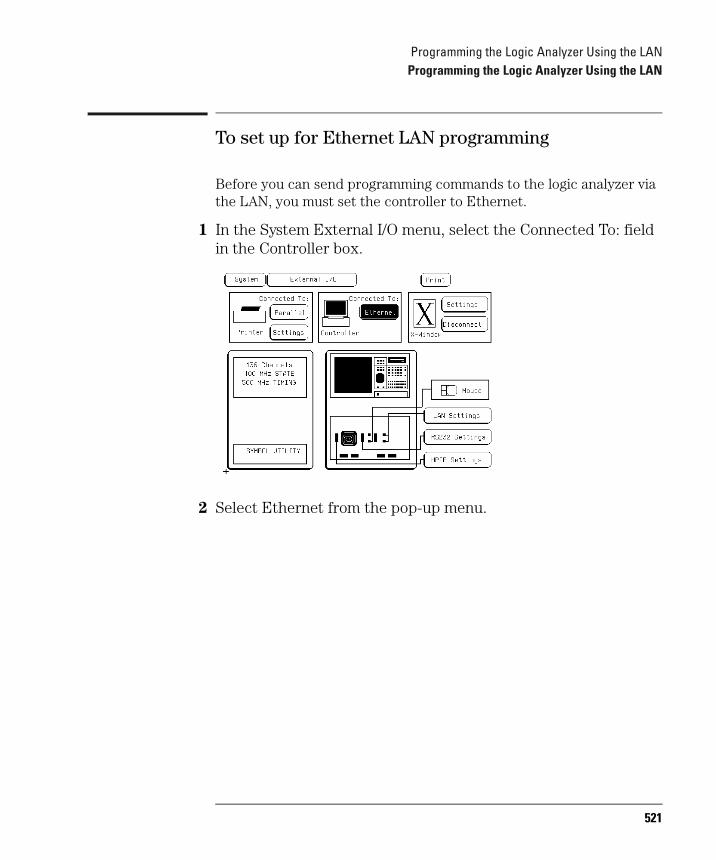
Programming the Logic Analyzer Using the LANProgramming the Logic Analyzer Using the LAN
To set up for Ethernet LAN programming
Before you can send programming commands to the logic analyzer via the LAN, you must set the controller to Ethernet.
1 In the System External I/O menu, select the Connected To: field in the Controller box.
2 Select Ethernet from the pop-up menu.
521
Programming the Logic Analyzer Using the LANProgramming the Logic Analyzer Using the LAN
To enter commands directly using telnet
The syntax of the telnet command is:
telnet [symbolic name|IP address] 5025
The symbolic name is the host name of the logic analyzer as set up by your system administrator. Typically, this name is found in the hosts file or returned by a name server. It is equivalent to the logic analyzer's IP address.
5025 is the port identification number of the logic analyzer's command parser socket. It must be specified because the logic analyzer is not a fully functional telnet server. If you forget to specify the port, you will get a connection refused message:
$ telnet 1670sysTrying...telnet: Unable to connect to remote host: Connection refused
To enter commands directly using telnet, first open a telnet connection using port 5025. A brief message appears confirming the connection, and telling you how to break the telnet connection:
$ telnet 1670sys 5025Trying...Connected to 1670sys.col.hp.comEscape character is '^]'.
When you connect to the logic analyzer, there is no prompt. Type logic analyzer commands; query results appear on the next line. When you are done, break the telnet connection using the escape character, and type "quit".
See the detailed example on the next page.
522
Programming the Logic Analyzer Using the LANProgramming the Logic Analyzer Using the LAN
Example Programming the logic analyzer over a telnet connection
To connect to the logic analyzer named 1670sys, enter:
$ telnet 1670sys 5025
The computer responds with:
Trying...Connected to 1670sys.col.hp.com.Escape character is '^]'.
The connection was successful. Because the analyzer does not provide a prompt, start entering programming commands. Typical commands might be:
:system:header on :system:longform on:select 1 :menu? MENU 1,3 :system:dsp 'Triggering on memory violation':system:print screen
The small program above turns on the header and longform for query responses, selects the analyzer, checks which menu it is on, creates a title for that screen, and then prints it to the default printer.
When you are done, close the telnet connection. Enter the escape character to get the telnet prompt. The escape character (Control and "]" in this example) does not print.
telnet> quit
The telnet connection closes and you see your regular prompt.
Connection closed.$
523
Programming the Logic Analyzer Using the LANProgramming the Logic Analyzer Using the LAN
To write programs that open the command parser socket
The command parser socket of the logic analyzer is 5025.
Connection to the command parser socket is, by definition, a control user connection. Because only one control user connection is allowed, you will not be able to open the command parser socket if someone else is accessing the logic analyzer's file system as the control user.
Example The following C program opens a socket and sends the *IDN query command to request the instrument's identity.
#include <stdio.h>#include <sys/types.h>#include <sys/socket.h>#include <netinet/in.h>
typedef struct sockaddr_in tdSOCKET_ADDR;
#define PARSER_PORT 5025#define SERV_HOST_ADDR "15.10.96.12"#define PARSER_BUFFER_SIZE 100
char receiveBuffer[PARSER_BUFFER_SIZE], *cmdString = "*IDN?\r\n" ;
main ()
int sockfd, port; tdSOCKET_ADDR serv_addr; char *addr;
/* Initialize a server socket */ port = PARSER_PORT; addr = SERV_HOST_ADDR ; serv_addr.sin_family = AF_INET; serv_addr.sin_addr.s_addr = inet_addr ( addr ); serv_addr.sin_port = htons ( port );
524

Programming the Logic Analyzer Using the LANProgramming the Logic Analyzer Using the LAN
/* Create an endpoint for communication */ sockfd = socket( AF_INET, SOCK_STREAM, 0 );/* Initiate a connection on the created socket */ connect(sockfd,(tdSOCKET_ADDR *)&serv_addr, sizeof (serv_addr));/* Send a message from the created socket */ send ( sockfd, cmdString, strlen ( cmdString ), 0 ); /* Receive a message from the 16500B socket */ recv(sockfd,receiveBuffer,sizeof(receiveBuffer),0 ); printf ( "%s\n", receiveBuffer ); close ( sockfd );
525

Programming the Logic Analyzer Using the LANProgramming the Logic Analyzer Using the LAN
526
21
LAN Concepts
527
LAN ConceptsLAN Concepts
LAN ConceptsThis chapter describes:
• Directory structure of the logic analyzer's file system
• Dynamic files
• New fields in the logic analyzer's system menus
528

LAN ConceptsLAN Concepts
Directory structure of the logic analyzer's file system
Logic Analyzer Directory Structure
setup.raw. Binary configuration files. You can save and restore configurations by copying these files.
\slot_x. Analyzer and oscilloscope subdirectories. All 1670G-series logic analyzers have a \slot_a directory for the state/timing analyzer. The 1670G-series with the oscilloscope option also have a \slot_b directory for the oscilloscope.
\slot_x\data.raw. Binary measurement data files. You can save and restore measurement data by copying these files.
\system\disk\hard. Same directory structure as System Hard Disk menu.
\system\disk\flexible. Same directory structure as System Flexible Disk menu.
529

LAN ConceptsLAN Concepts
\system\graphics. Image files for the current screen in TIFF, PCX, and Encapsulated PostScript formats.
\status. Status information.
The directory structure of the logic analyzer is fixed. You cannot create or delete directories or files except under the local hard and flexible disk directories.
Analyzer (\slot_a) Subdirectories and Files
The slot_a directory contains a subdirectory called data.asc that contains ASCII measurement data.
There are two subdirectories attached to the data.asc directory, one for each of the two analyzers in the logic analyzer (if they are turned on in the Configuration Menu). The default names of these subdirectories are machine1 and machine2, but they will change whenever the analyzer names are changed in the Configuration Menu.
Analyzer Directory Structure
Root
slot_a
data.asc
analyzer 1 analyzer 2
label 1.txtlabel 2.txtlabel 3.txt
.
.
.1st_line.txtline_num.txttime_abs.txt
label 1.txtlabel 2.txtlabel 3.txt
.
.
.1st_line.txtline_num.txtstate_abs.txt
system status
programsetup.rawdiskgraphics
frame.txtmount.txtsystem.txt
530
LAN ConceptsLAN Concepts
Label Data Files: \slot_a\data.asc\analyzer name\label.txt.
Both analyzer subdirectories contain files corresponding to the labels you have set up in that analyzer's Format Menu. These files contain the current measurement data for the channels assigned to each label.
Both state and timing data are available, and both kinds of data are represented as a column of values. The numeric base ƒ hex, binary, etc. ƒ in these files is the same as the base that is currently set in the Listing Menu.
The 1st_line.txt File. The 1st_line.txt file lists the number of the first line of the most recent data acquisition.
This file shows the number of states that occur before the trigger state, which is always state zero (at line number 0). You can use this information to align data from different measurements.
Time Tag and State Tag Data. If time tags have been turned on, the time_abs.txt file contains a column of time values for the most current state or timing measurement. Timing analyzers always have a time_abs.txt file.
If state tags have been turned on, the state_abs.txt file contains a column of state count values for the most current state measurement.
Line Numbers. The line_num.txt file contains line numbers corresponding to the lines of data in a state listing.
531
LAN ConceptsLAN Concepts
Dynamic files
The logic analyzer's file system uses dynamic files for configuration information and data. This means that applications such as File Manager or a spreadsheet cannot determine the size of the files until they are retrieved.
When you view the file statistics for these files, you will see file sizes of 0 bytes or 1 byte. The 0-byte size indicates that the file is empty. The 1-byte size indicates that there is information in the file. If you transfer the file of interest to your PC or workstation, you will be able to see the actual file size.
Known Incompatibilities
Some operating systems and applications may exhibit unexpected behavior when working with the dynamic files from the logic analyzer. The "%complete" display may appear incorrect during file transfers. This does not affect the transfer or the contents of the file. Once you have saved the file in your local environment, the correct "% complete" will be displayed during future retrievals.
Your applications might only retrieve one or two characters from a file that you believe has many more characters in it. To work around this problem, copy the file that you want to work with from the logic analyzer to your local computer. Use the local copy as your working copy.
SUN Operating Systems
The file copy commands in the SUN workstation and Solaris operating systems will not work with the dynamic files like those used in the logic analyzer. You can use the dd command instead of using the cp or cat commands.
532

LAN ConceptsLAN Concepts
LAN-related fields in the logic analyzer's menus
When your logic analyzer has LAN, several additional menu choices are available. These fields allow you to set up your LAN port and configure the logic analyzer.
Controller Connection
You can set your logic analyzer to be controlled over the network. In the System External I/O menu, when you select the Connected To: field in the controller box the choices are now GPIB, RS-232C, and Ethernet.
X-Window Box
LAN adds an X-Window box to the System External I/O menu. The X-Window box has two fields for configuring an X connection. Chapter3, "Using the X Window Interface," explains how to set up an X Window connection.
LAN Settings
LAN adds a LAN Settings box to the System External I/O menu so that you can configure the logic analyzer to work with your network. The LAN Settings menu is explained in Chapter1, "Connecting and Configuring."
533
LAN ConceptsLAN Concepts
Time Zone Field
With LAN, a field labeled "Time Zone" appears in the Real Time Clock setup menu. The Real Time Clock setup menu is accessed by selecting the Real Time Clock Adjustments field in the System Utilities menu.
This field enables you to specify the time difference between your local time and Greenwich Mean Time (Universal Coordinated Time) for network operations. The Time Zone value can be varied from -12 to +12. The number represents the number of hours difference between your local time zone and Greenwich Mean Time. The time value is used to timestamp files when they are stored to disk or transferred to your computer, and to correctly display the time data of the logic analyzer files when you NFS-mount the logic analyzer.
534
22
Troubleshooting the LAN Connection
535

Troubleshooting the LAN ConnectionTroubleshooting the LAN Connection
Troubleshooting the LAN ConnectionThis chapter provides troubleshooting information for the LAN connection. It is arranged in three sections:
• Troubleshooting the initial connection
• Solutions to common problems
• Getting service support
536

Troubleshooting the LAN ConnectionTroubleshooting the Initial Connection
Troubleshooting the Initial ConnectionGetting the logic analyzer to work with your network often requires detailed knowledge of your local network software. This section attempts to help you with some common problems, but because of the wide variety of network software available it cannot cover all problems you may encounter.
Assess the problem
The LAN interface does not need or include any utilities or proprietary driver software. The logic analyzer LAN interface was designed to operate with common network utilities and drivers.
Either a hardware problem or a software problem can prevent the logic analyzer's remote file server from communicating over the LAN.
NOTE: Single server/single client network (point-to-point)You can connect the logic analyzer to a single server/single client network. In this configuration, the client is running an NFS application program. If you have difficulties, check the troubleshooting procedures included with the documentation for both the NFS application program and the communications controller first. If the NFS application program is running in an MS Windows environment, then also check the MS Windows documentation.
Timeout errors
Error messages such as "Device Timeout," "File Timeout," "Operation Timeout," or other similar messages from workstations or PCs indicate timeout problems with the computer. To increase your timeout period, refer to your computer documentation for instructions.
537
Troubleshooting the LAN ConnectionTroubleshooting the Initial Connection
Packets routinely lost
If packets are routinely lost, proceed to the troubleshooting section in this chapter relating to your network.
Problems transferring or copying files
Copying files out of the logic analyzer
• If you have problems copying files out of the logic analyzer, you might be experiencing timeout problems. See the timeout section on the previous page.
• If you only receive 1 byte back when copying files, refer to "Dynamic Files" later in this chapter.
Copying files into the logic analyzer
• If you have problems copying files into the logic analyzer, such as copying setup or data to change a configuration, then check the File Timeout setting in the LAN Settings menu. Refer to "Configure the network addresses" in Chapter 1 for more information.
Communications not established
If you have just installed and configured the LAN interface and you have never been able to read the logic analyzer remote file server directory, go directly to the troubleshooting section relating to your network in this chapter.
If you have been able to read the logic analyzer remote file server directory and now cannot do so, check the following:
• Has any hardware been added or moved on your network? This includes adding or removing any workstations or peripherals, or changing any cabling.
• Have software applications been added to the network?
538
Troubleshooting the LAN ConnectionTroubleshooting the Initial Connection
• Have any configuration files been modified?
• Have any of the following files been deleted or overwritten?UNIX:
/etc/hosts/etc/inetd.conf/etc/services
PCs:dependent network files
If you know or suspect that something has changed on your network, check the changes and adjust the configuration for the LAN interface using the procedures in Chapter 1. Otherwise, proceed to the troubleshooting section in this chapter relating to your network.
539

Troubleshooting the LAN ConnectionTroubleshooting the Initial Connection
Troubleshooting in a workstation environment
1 Verify the communications link.
Verify the communications link between the computer and the logic analyzer remote file server using the ping utility.
ping [hostname|IP Address] 64 10
Hostname is the name assigned to the logic analyzer remote file server in the node names database (usually /etc/hosts). Most workstation platforms permit an IP address to be used in place of hostname. In the example above, packet size is 64 and 10 packets are transmitted.
To aid in troubleshooting, go to the LAN Settings Ethernet Statistics menu on the logic analyzer. You can view transmit and receive activity on this menu. If needed, refer to "Network Status Information" in this section for more information about the Ethernet Statistics menu.
• Normal ResponseA normal response to the ping will be a total of 9, 10, or possibly 11 packets received with a minimal average of round-trip time. The minimal average will be different from network to network. LAN traffic will cause the round-trip time to vary widely.Because the number of packets received depends on your network traffic and integrity, the normal number might be different for your network.For every packet transmitted and received because of the ping command, the Transmit Successful and Receive Successful fields in the logic analyzer Ethernet Statistics menu increases by 1.Go to step 2, "Attempt a remote NFS mount."
540

Troubleshooting the LAN ConnectionTroubleshooting the Initial Connection
• Error MessagesIf error messages appear, then check the command syntax before continuing with the troubleshooting. If the syntax is correct, then resolve the error messages using your network documentation.If an unknown host error message appears, then check the node names database (usually /etc/hosts) to see that the hostname and IP address are correctly entered.
• No responseNo packets received indicates no response from a ping. If there is no response, type in the IP address with the ping command. Check that the typed address matches the IPaddress assigned in the LAN Settings menu, then check the other addresses in the menu.Check that the hostname and IP address are correctly entered in the node names database on your workstation (usually /etc/hosts).Ping each node along the route between your workstation and the logic analyzer, starting with the your workstation. Ping each gateway, then attempt a ping of the remote file server.If the logic analyzer still does not respond to ping, then you should suspect a hardware problem with the logic analyzer. To check the logic analyzer performance, refer to "Verify the logic analyzer performance" in this section.
• Intermittent ResponseIf you received 1 to 8 packets back, there is probably a problem with the network. Because the number of packets received depends on your network traffic and integrity, the number might be different for your network.Use a LAN analyzer or LAN management software to monitor activity and determine where bottlenecks or other problems are occurring. The logic analyzer will still function, but communications over the LAN will be slower.
541
Troubleshooting the LAN ConnectionTroubleshooting the Initial Connection
Troubleshooting in an MS-DOS environment
1 Verify the communications link.
Verify the communications link between the PC and the logic analyzer using the ping utility or other similar echo request utility.
To aid in troubleshooting, go to the Ethernet Statistics menu under LAN Settings on the logic analyzer. You can view transmit and receive activity on this menu. If needed, refer to "Network Status Information" in this chapter for more information about the Ethernet Statistics menu.
If the ping utility is not available on the PC, then this is an indication that the PC-based NFS software is not properly installed. Reinstall the PC-based NFS software and attempt to verify the communications link.
The syntax of the ping command varies with the NFS software used. Usually, the command requires at least the IP address. If the syntax permits a specified number of echo requests, then specify 10 as the number of echo requests. Refer to the NFS software documentation for more information.
ping [IP address] 10
• Normal ResponseA normal response to the ping will be a total of 9, 10, or possibly 11 packets received if 10 echo requests were specified. Because the number of packets received depends on your network traffic and integrity, the normal number might be different for your network.For every packet transmitted and received because of the ping command, the Transmit Successful and Receive Successful fields in the Ethernet Statistics menu increases by 1.Go to step 2, "Attempt a remote NFS mount."
542
Troubleshooting the LAN ConnectionTroubleshooting the Initial Connection
• Error MessagesIf error messages appear, then check the command syntax before continuing with the troubleshooting. If the syntax is correct, then resolve the error messages using your NFS documentation.Certain PC-based NFS software packages permit the use of hostname in place of the IP address. In this case, if an unknown host error message appears, then check the node names database to see that the hostname and IP address are correctly entered.Refer to the NFS software documentation for specific information on any error messages.
• No responseNo packets received indicates no response from a ping.If there is no response, type in the IP address with the ping command. Check that the typed address matches the IPaddress assigned in the LAN Settings menu, then check the other addresses in the menu.Check that the hostname and IP address are correctly entered in the node names database and that the IP address matches the IP address assigned in the LAN Settings menu.If the logic analyzer still does not respond to ping, then the problem is possibly in the logic analyzer hardware. To check the logic analyzer, refer to "Verify the logic analyzer performance" in this chapter.
• Intermittent ResponseOn a multiclient network, receiving 1 to 8 packets indicates a problem with the network. Because the number of packets received depends on your network traffic and integrity, the number might be different for your network.Use a LAN analyzer or LAN management software to monitor activity and determine where bottlenecks or other problems are occurring. The logic analyzer still functions, but communications over the LAN will be slower.On a single-client/single-server network, the most likely cause of intermittent response to an echo request is a hardware problem with the LAN module installed in the PC, the cable, or the logic analyzer. To check the logic analyzer, refer to "Verify the logic analyzer performance" in this chapter.
543
Troubleshooting the LAN ConnectionTroubleshooting the Initial Connection
Troubleshooting in an MS Windows environment
1 Verify the communications link.
Verify the communications link between the PC and the logic analyzer using the ping utility or other similar echo request utility.
To aid in troubleshooting, go to the Ethernet Statistics menu under LAN Settings on the logic analyzer. You can view transmit and receive activity on this menu. If needed, refer to "Network Status Information" in this chapter for more information about the Ethernet Statistics menu.
If the ping utility is not available on the PC (the icon does not appear), then this is an indication that the NFS software is not properly installed. Reinstall the NFS software and attempt to verify the communications link.
The syntax of the ping command varies with the NFS software used. Usually, the command requires at least the IP address. If the syntax permits a specified number of echo requests, then specify 10 as the number of echo requests. Refer to your NFS software documentation for more information.
• Normal ResponseA normal response to the ping will be a total of 9, 10, or possibly 11 packets received if 10 echo requests were specified. Because the number of packets received depends on your network traffic and integrity, the normal number might be different for your network.For every packet transmitted and received because of the ping command, the Transmit Successful and Receive Successful fields in the Ethernet Statistics menu increases by 1.Go to step 2, "Attempt a remote NFS mount."
544
Troubleshooting the LAN ConnectionTroubleshooting the Initial Connection
• Error MessagesIf error messages appear, then check the command syntax before continuing with the troubleshooting. If the syntax is correct, then resolve the error messages using your NFS documentation.Certain NFS software packages permit the use of hostname in place of the IP address. In this case, if an unknown host error message appears, then check the node names database to see that the hostname and IP address are correctly entered.Refer to your NFS documentation for specific information on any error messages.
• No responseNo packets received indicates no response from a ping.If there is no response, type in the IP address with the ping command. Check that the typed address matches the IPaddress assigned in the LAN Settings menu, then check the other addresses in the menu.Check that the hostname and IP address are correctly entered in the node names database and that the IP address matches the IP address assigned in the LAN Settings menu.If the logic analyzer still does not respond to ping, then the problem is possibly in the logic analyzer hardware. To check the logic analyzer, refer to "Verify the logic analyzer performance" in this chapter.
• Intermittent ResponseOn a multiclient network, receiving 1 to 8 packets indicates a problem with the network. Because the number of packets received depends on your network traffic and integrity, the number might be different for your network.Use a LAN analyzer or LAN management software to monitor activity and determine where bottlenecks or other problems are occurring. The logic analyzer still functions, but communications over the LAN will be slower.On a single-client/single-server network, the most likely cause of intermittent response to an echo request is a hardware problem with the LAN module installed in the PC, the cable, or the logic analyzer. To check the logic analyzer, refer to "Verify the logic analyzer performance" in this chapter.
545
Troubleshooting the LAN ConnectionTroubleshooting the Initial Connection
Verify the logic analyzer performance
The logic analyzer performance verification (self-test) is divided into two sections. The first section tests the physical connections such as the cable and termination. The second section tests the internal functions of the LAN interface. When both sections of the self-test have finished, a status message appears in the LAN Test field. The status message indicates whether the test passed, if a failure occurred, and which section failed.
The physical connection test depends on the LAN topology used. If ThinLAN is used, then a test transmission signal is transmitted over the LAN. If a reply is received, then the physical connection is considered good. If EtherTwist (10Base-T) is used, then the logic analyzer will listen for the heartbeat signal from the LAN. If a heartbeat is received, then the physical connection is considered good.
The second section is tested using internal loopback features of the LAN hardware. Transmitted packets are looped back to the receive circuit of the LAN board. When the looped-back packets are received, they are processed like a packet received from a remote client or server. If the looped-back packet is recognized and processed, then the LAN board and the LAN software are considered good.
Perform the following check before beginning the procedure.
Check all network cables and connectors. Verify that all cables are properly connected.
546
Troubleshooting the LAN ConnectionTroubleshooting the Initial Connection
Procedure
This procedure verifies the performance of the LAN interface. To check logic analyzer performance, refer to the logic analyzer's Service Guide.
1 Go to the System External I/O menu.
2 Verify that the LAN Settings box and the X-Window box are available.
If these boxes appear, go to the next step. If the boxes are not there, then the LAN interface is not properly installed. If the screen is completely blank, then there might be loose cables.
3 Go to the System Test menu.
4 Select Load Test System.
If you do not have a copy of the performance verification files on the hard disk, you need to insert the disk containing the performance verification files into the flexible disk drive.
5 Select Analy PV, and then select Sys PV from the pop up.
6 Select External I/O, and then select System Test from the pop up.
7 Select LAN Test, then select Run.
8 Verify that the tests pass.
If all of the tests pass, then go to the next step. If any of the tests fail, then the LAN hardware is suspect.
The status number in the LAN Test field indicates whether the LAN hardware or software caused the failure.
• To troubleshoot the failure using the status number, note the number, then compare it with the status number descriptions and perform the recommended action. Refer to "Status Number" on the next few pages for status number descriptions and recommended actions.
• To verify the LAN hardware, check that the LAN cable is good and that all signal lines in the cable have electrical integrity.
547

Troubleshooting the LAN ConnectionTroubleshooting the Initial Connection
9 Exit the Test System.
a Select System Test, then select Exit Test from the pop up.
b Select Exit Test System.
Status Number
When you run the LAN Test, the test menu reports a status number. The following figure shows the bit positions of the hexidecimal status word.
A "1" in a bit position signifies that the bit is set and the test failed.
A "0" in a bit position signifies that the bit is not set and the test passed.
Status Word
548
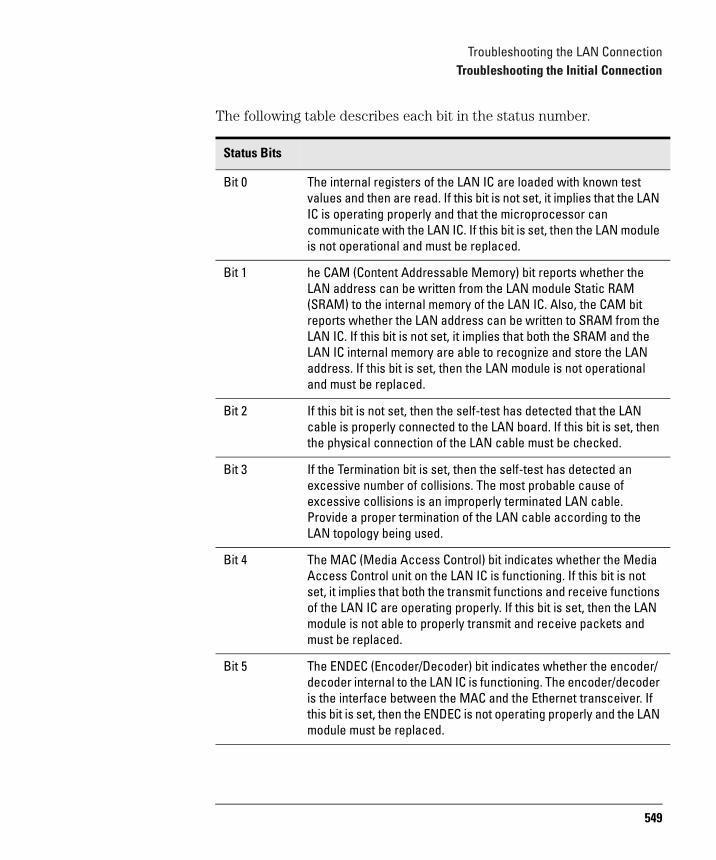
Troubleshooting the LAN ConnectionTroubleshooting the Initial Connection
The following table describes each bit in the status number.
Status Bits
Bit 0 The internal registers of the LAN IC are loaded with known test values and then are read. If this bit is not set, it implies that the LAN IC is operating properly and that the microprocessor can communicate with the LAN IC. If this bit is set, then the LAN module is not operational and must be replaced.
Bit 1 he CAM (Content Addressable Memory) bit reports whether the LAN address can be written from the LAN module Static RAM (SRAM) to the internal memory of the LAN IC. Also, the CAM bit reports whether the LAN address can be written to SRAM from the LAN IC. If this bit is not set, it implies that both the SRAM and the LAN IC internal memory are able to recognize and store the LAN address. If this bit is set, then the LAN module is not operational and must be replaced.
Bit 2 If this bit is not set, then the self-test has detected that the LAN cable is properly connected to the LAN board. If this bit is set, then the physical connection of the LAN cable must be checked.
Bit 3 If the Termination bit is set, then the self-test has detected an excessive number of collisions. The most probable cause of excessive collisions is an improperly terminated LAN cable. Provide a proper termination of the LAN cable according to the LAN topology being used.
Bit 4 The MAC (Media Access Control) bit indicates whether the Media Access Control unit on the LAN IC is functioning. If this bit is not set, it implies that both the transmit functions and receive functions of the LAN IC are operating properly. If this bit is set, then the LAN module is not able to properly transmit and receive packets and must be replaced.
Bit 5 The ENDEC (Encoder/Decoder) bit indicates whether the encoder/decoder internal to the LAN IC is functioning. The encoder/decoder is the interface between the MAC and the Ethernet transceiver. If this bit is set, then the ENDEC is not operating properly and the LAN module must be replaced.
549

Troubleshooting the LAN ConnectionTroubleshooting the Initial Connection
Status Bits (continued)
Status Bits
Bit 6 The TRANS (Transceiver, such as Ethernet transceiver) bit indicates whether the circuitry between the LAN IC and the LAN cable is functioning. If this bit is not set, then the path between the LAN cable and the LAN IC is operating properly. If this bit is set, then either the CPU board or the I/O board must be replaced.
Bit 7 Timeout bit. If the Timeout bit is set, then bits 4, 5, or 6 will also be set. Refer to the appropriate bit for a suggested course of action.
Bit 8 The Tx bit indicates whether the transmission portion of the MAC, ENDEC, or TRANS test failed. Therefore, the Tx bit is used in conjunction with bits 4, 5, and 6. Refer to the appropriate bit for the suggested course of action.
Bit 9 The Rx bit indicates whether the receive portion of the MAC, ENDEC, or TRANS test failed. The Rx bit is used in conjunction with bits 4, 5, and 6. Refer to the appropriate bit for the suggested course of action.
Bit 10 The Parameters bit indicates the integrity of the LAN module self-test parameters. If this bit is not set, then the parameters sent to the self-test routine are correct. If this bit is set, then contact your nearest Agilent Technologies Sales and Service Office.
Bit 11 The EPROM that is used to hold the Ethernet address, IP address, and gateway address has been corrupted. If this bit is set, the LAN board must be replaced.
Bits 12-15 Not Used
550
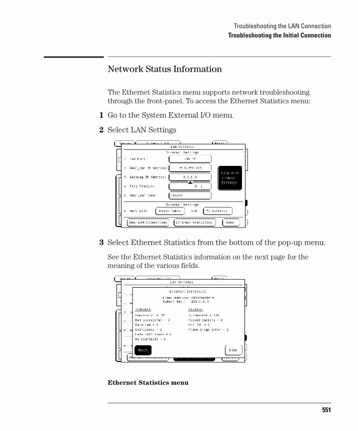
Troubleshooting the LAN ConnectionTroubleshooting the Initial Connection
Network Status Information
The Ethernet Statistics menu supports network troubleshooting through the front-panel. To access the Ethernet Statistics menu:
1 Go to the System External I/O menu.
2 Select LAN Settings
3 Select Ethernet Statistics from the bottom of the pop-up menu.
See the Ethernet Statistics information on the next page for the meaning of the various fields.
Ethernet Statistics menu
551
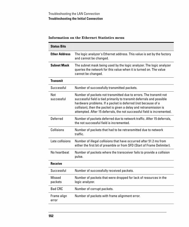
Troubleshooting the LAN ConnectionTroubleshooting the Initial Connection
r
.
,
.
Information on the Ethernet Statistics menu
Status Bits
Ether Address The logic analyzer's Ethernet address. This value is set by the factoryand cannot be changed.
Subnet Mask The subnet mask being used by the logic analyzer. The logic analyzequeries the network for this value when it is turned on. The value cannot be changed.
Transmit
Successful Number of successfully transmitted packets.
Not successful
Number of packets not transmitted due to errors. The transmit not successful field is tied primarily to transmit deferrals and possible hardware problems. If a packet is deferred (not because of a collision), then the packet is given a delay and retransmission is attempted. After 15 deferrals, the not successful field is incremented
Deferred Number of packets deferred due to network traffic. After 15 deferralsthe not successful field is incremented.
Collisions Number of packets that had to be retransmitted due to network traffic.
Late collisions Number of illegal collisions that have occurred after 51.2 ms from either the first bit of preamble or from SFD (Start of Frame Delimiter)
No heartbeat Number of packets where the transceiver fails to provide a collisionpulse.
Receive
Successful Number of successfully received packets.
Missed packets
Number of packets that were dropped for lack of resources in the logic analyzer.
Bad CRC Number of corrupt packets.
Frame align error
Number of packets with frame alignment error.
552
Troubleshooting the LAN ConnectionSolutions to Common Problems
Solutions to Common ProblemsThis section describes common problems you may encounter when using the logic analyzer LAN. It assumes you have been able to connect to the logic analyzer in the past. If this is not so, refer to the previous section first.
If you cannot connect to the logic analyzer
If you suspect a bad LAN connection between your computer and the logic analyzer, you can verify the network connection by using the ping command or another similar echo request utility.
If a bad connection is revealed:
Make sure the logic analyzer is on.
Check the physical connection to the LAN.
Make sure the Internet (IP) Address of the logic analyzer is set up correctly in the LAN Settings menu under System External I/O.
If the logic analyzer and the computer are on different networks or subnets, make sure the Gateway Address in the LAN Settings menu is set to the address of the gateway machine. Get the address of gateway machine from your system administrator.
553
Troubleshooting the LAN ConnectionSolutions to Common Problems
If you cannot mount the logic analyzer file system
If you get a "device busy" message:
Make sure that another user is not already accessing the file system as the control user or connected to the command parser socket.
If you get a "stale NFS file handle" message:
Unmount the file system and try mounting again. The likely cause of this error is turning off power to the logic analyzer before unmounting.
If you get a "server not responding" message:
If the power to the logic analyzer was just turned on, make sure that you wait 15 seconds after the Analyzer Configuration menu is displayed before attempting the mount.
Verify the LAN connection between your computer and the logic analyzer. Refer to "If you cannot connect to the logic analyzer" earlier in this section.
If you cannot access the file system via ftp
If you get a "connection refused" message:
If the power to the logic analyzer was just turned on, make sure that you wait 15 seconds after the Analyzer Configuration menu is displayed before attempting the connection.
If you get a "connection timed out" message:
Verify the LAN connection between your computer and the logic analyzer. Refer to "If you cannot connect to the logic analyzer" earlier in this section.
554
Troubleshooting the LAN ConnectionSolutions to Common Problems
If you get an "already mounted" or "no more mounts available" message:
If you are trying to access the file system as the control user, try accessing the file system as the data user instead. If another user is currently accessing the logic analyzer file system as the control user, you will not be able to access the file system as the control user.
If you cannot start the XWindow interface
If you get an "Unable to open window on <IP address>.<display>.<screen>" message:
Make sure that the logic analyzer has permission to open a window on the Xserver. For example, you may have to enter an "xhost +<IPaddress>" command on your Xserver machine.
If your X Window looks odd
If certain of the symbols, such as the activity indicators, look odd:
Load the X Window fonts. See "To load custom fonts" on page 505.
If the X Window is only using two or three colors:
Release colors by closing down some applications, and restart your X Windows session.
555
Troubleshooting the LAN ConnectionSolutions to Common Problems
If you cannot copy files from the logic analyzer
If you can only copy a few bytes of a file:
Copy the file of interest to your PC or workstation, and use the new, local copy as your working copy. Some applications cannot work directly with the dynamic files from the logic analyzer.
If you are on a UNIX workstation, try using dd instead of cp.
If you cannot restore raw files
If the setup.raw and data.raw files seem to be ignored when you copy them to the logic analyzer:
Verify the LAN connection between your computer and the logic analyzer. Refer to "If you cannot connect to the logic analyzer" earlier in this section.
Change the file time-out. To change the time-out:
1 Go to the logic analyzer System External I/O menu.
2 Select the LAN Settings field.
3 Set the file time out.
A value of about 1.5 seconds should be sufficient. Set the time out to the minimum value that will allow network operations to work reliably.
556
Troubleshooting the LAN ConnectionSolutions to Common Problems
If you get an "operation timed-out" message
Check the LAN connection between the computer and logic analyzer. Refer to "If you cannot connect to the logic analyzer" in this section.
Increase the file time-out value on your PC or workstation.
If the logic analyzer begins to operate slowly
The logic analyzer may operate more slowly if multiple users are trying to use the system at the same time.
Check the number of network connections. Either copy the file \system\mount.txt to your local computer and view it with a text editor, or on the analyzer go to the LAN Settings menu and select Show LAN Connections. Check to see if many other users are currently connected to the system.
If the logic analyzer does not respond
When the logic analyzer is transmitting a large file such as a deep- memory acquisition or a screen image, or when it is transmitting a dynamic file, it does not respond. Please be patient.
If the analyzer does not respond after several minutes, cycle the power. It may take up to twenty minutes to transmit.
557
Troubleshooting the LAN ConnectionSolutions to Common Problems
If all else fails
Contact your system administrator.
If you still cannot solve the problem, contact an Agilent Technologies Service Center for repair information.
558

Troubleshooting the LAN ConnectionGetting Service Support
Getting Service SupportThis section provides information about support services.
Return to Agilent service
The benchtop logic analyzers default to return to Agilent Technologies service. With return to Agilent Technologies service, you return the equipment to your nearest Agilent Technologies service center for repair. During the warranty period, Agilent Technologies pays for parts and labor needed for repair. After the warranty period, you are billed for the parts and labor.
To arrange for Return to Agilent Technologies Service, contact your local Agilent Technologies service representative. In the United States, call 1-800-403-0801. In Japan call 81-426-56-7799.
Other local service representitives can be found on the World Wide Web at http://www.agilent.com/find/clservice under Contact Us.
559

Troubleshooting the LAN ConnectionGetting Service Support
560
Section 3
Symbol Utility
561

562
23
Symbol Utility Introduction
563
Symbol Utility IntroductionSymbol Utility Introduction
Symbol Utility IntroductionThe Symbol Utility provides you with a new way to view your logic analysis data. The Symbol Utility maps trace data onto meaningful, symbolic names. The symbols can include variable names, procedure or function names, and source file names and line numbers. The linkage between the symbol names and the trace data values comes from one of two sources:
• Object Module Format (OMF) files generated by your compiler and linker, or
• ASCII files that you create with a text editor
Using the symbol utility, you have two new capabilities:
• you can view symbols from OMF files in a logic analyzer state listing
• you can use the OMF symbols as trigger terms in a logic analyzer trigger specification.
NOTE: We assume that you are familiar with the operation of your logic analyzer. If not, refer to the Logic Analyzer Training Kit for information on how to use the logic analyzer interface or the appropriate User's Guide for details on the system menus and functions.
NOTE: Refer to your software tool documentation for information about how to generate OMF files during compilation and linking.
Equipment Required
• 1670G-series logic analyzer
564

Symbol Utility IntroductionSymbol Utility Introduction
Supported Symbol File Formats
The Symbol Utility will support OMF files in the following formats:
ELF/DWARF. This OMF is a portable format consisting of ELF (Executable and Linkable Format) and DWARF (Debugging Information Format) for various processors, including Intel 80960, PowerPC, and MIPS.
GPA. The General-Purpose ASCII file format, which can be used to provide symbols for an Object Module Format which is not explicitly supported. See the "General-Purpose ASCII Symbol File Format" on page 605 for more details.
Agilent-MRI IEEE-695. The OMF produced by Agilent Technologies and MRI cross-compilers and cross-assemblers. This format is fully supported by the Symbol Utility's IEEE-695 reader.
IEEE-695. This OMF is usually produced by language tools for non-Intel microprocessors. Some language tools which claim to output this format may deviate from the IEEE-695 standard in ways which make the OMF file unreadable by the Symbol Utility's reader.
OMF286. This OMF is produced by language tools for Intel 80x86 series and Pentium microprocessors running in real and/or protected mode. The supported OMF286 file types are Single-task Loadable and Bootloadable.
OMF386. This OMF is produced by language tools for Intel 80x86 series and Pentium microprocessors running in real and/or protected mode. The supported OMF386 file types are Loadable and Boot loadable.
565
Symbol Utility IntroductionSymbol Utility Introduction
OMF86. This OMF is produced by language tools for Intel 80x86 series and Pentium microprocessors running in real mode only.
OMF96. This OMF is produced by language tools for the Intel 80196 family of processors.
TI-COFF. This OMF is produced by language tools for Texas Instruments microprocessors.
566
Symbol Utility IntroductionSymbol Utility Introduction
Symbol Utility section overview
The chapters in the Symbol Utility section of this User’s Guide provides a detailed description of the features. The following is a brief description of each chapter.
Getting Started. Describes how to locate the menus associated with the Symbol Utility.
Using the Symbol Utility. Describes how to use the Symbol Utility to perform common tasks like triggering on an OMF symbol.
Features and Functions. Describes the features and functions of the Symbol Utility. It also provides a detailed description of the General-Purpose ASCII file format.
567

Symbol Utility IntroductionSymbol Utility Introduction
568
24
Getting Started with the Symbol Utility
569
Getting Started with the Symbol UtilityGetting Started with the Symbol Utility
Getting Started with the Symbol UtilityYou can use the OMF Symbol Load menu to load Object Module Format (OMF) symbol files into the analyzer. Once you have loaded the files, you can view the symbols in the Listing and Waveform menus. You can use the OMF Symbol browser menu to create trigger conditions for your logic analyzer.
See Also The Logic Analyzer Training Kit for information on how to use the logic analyzer interface.
The Logic Analyzer section of this book for information on the features and functions of the logic analyzer.
570
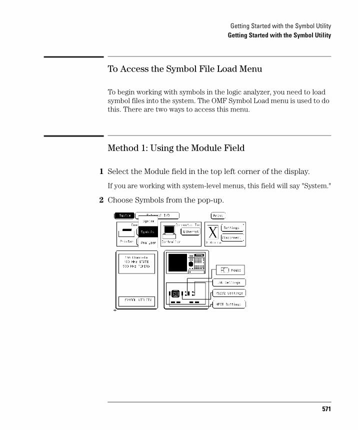
Getting Started with the Symbol UtilityGetting Started with the Symbol Utility
To Access the Symbol File Load Menu
To begin working with symbols in the logic analyzer, you need to load symbol files into the system. The OMF Symbol Load menu is used to do this. There are two ways to access this menu.
Method 1: Using the Module Field
1 Select the Module field in the top left corner of the display.
If you are working with system-level menus, this field will say "System."
2 Choose Symbols from the pop-up.
571
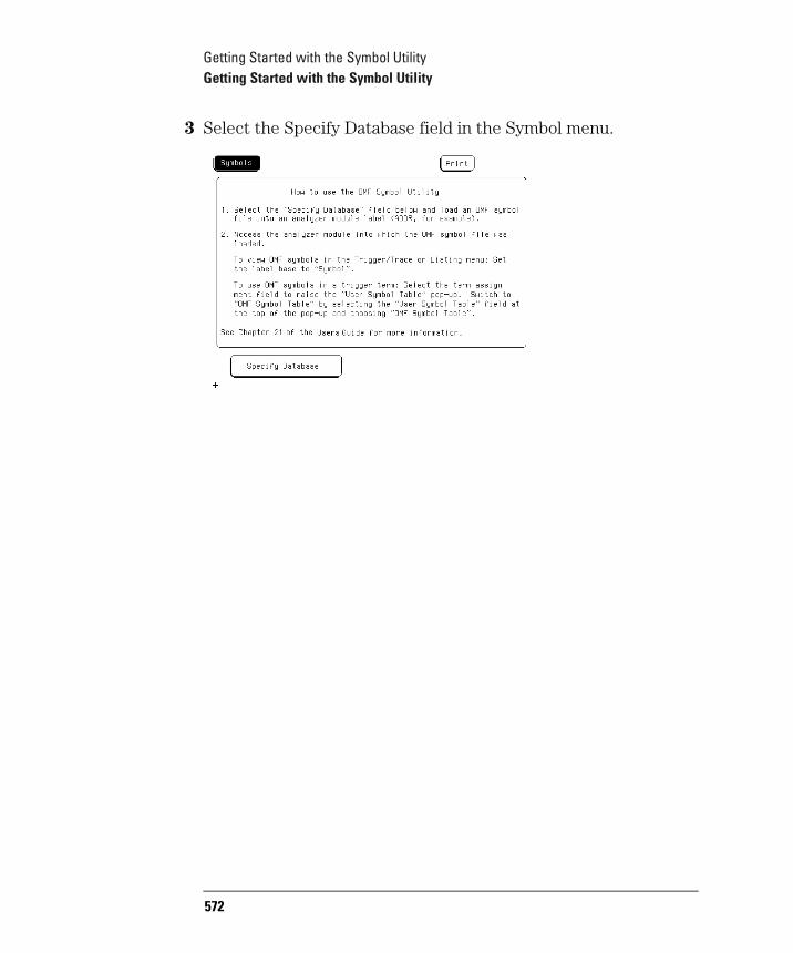
Getting Started with the Symbol UtilityGetting Started with the Symbol Utility
3 Select the Specify Database field in the Symbol menu.
572

Getting Started with the Symbol UtilityGetting Started with the Symbol Utility
Method 2: Using the Symbol Field in the Format Menu
1 Go to the Analyzer Format menu.
2 In the Format menu, select the Symbols field.
3 In the Symbols pop-up, select the large field at the top of the display. Choose OMF Symbol Table from the pop-up.
573
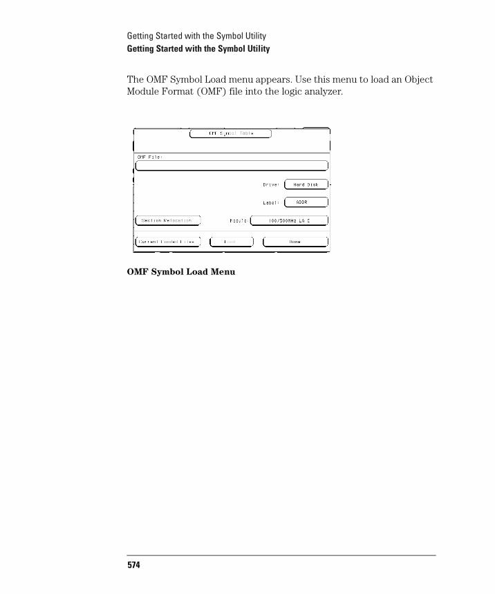
Getting Started with the Symbol UtilityGetting Started with the Symbol Utility
The OMF Symbol Load menu appears. Use this menu to load an Object Module Format (OMF) file into the logic analyzer.
OMF Symbol Load Menu
574
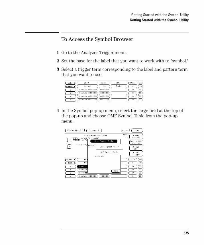
Getting Started with the Symbol UtilityGetting Started with the Symbol Utility
To Access the Symbol Browser
1 Go to the Analyzer Trigger menu.
2 Set the base for the label that you want to work with to "symbol."
3 Select a trigger term corresponding to the label and pattern term that you want to use.
4 In the Symbol pop-up menu, select the large field at the top of the pop-up and choose OMF Symbol Table from the pop-up menu.
575
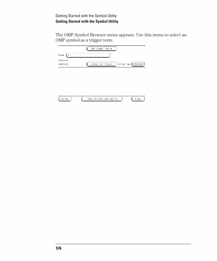
Getting Started with the Symbol UtilityGetting Started with the Symbol Utility
The OMF Symbol Browser menu appears. Use this menu to select an OMF symbol as a trigger term.
576
25
Using the Symbol Utility
577
Using the Symbol Utility
To generate a symbol file
In order to view symbols from your software in the Listing or Waveform menus of the logic analyzer, you need to create a symbol file in one of the formats that are supported by the Symbol Utility. If your language tools cannot generate an OMF symbol file which is compatible with the Symbol utility, you may create a symbol file in the General-Purpose ASCII (GPA) file format.
1 Compile, assemble, and link your program using the "generate symbol file" option of your language tools.
2 Transfer the DOS-formatted symbol file to the logic analyzer. You can put the file on a flexible disk, or use a LAN interface to transfer the file directly to the hard disk.
NOTE: If you need help creating OMF files, refer to your software tool documentation for information about how to generate OMF files during compilation and linking.
See also "The General-Purpose ASCII File Format" on page 605 for a complete description of the ASCII symbol file format.
"Supported Symbol File Formats," on page 565 for a list of the symbol file formats that are supported.
578
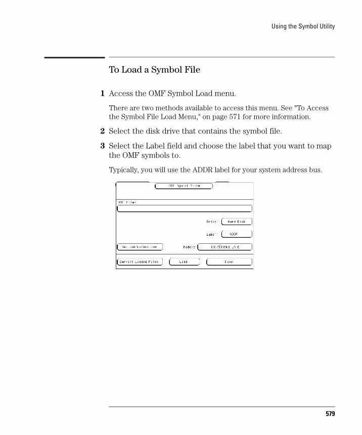
Using the Symbol Utility
To Load a Symbol File
1 Access the OMF Symbol Load menu.
There are two methods available to access this menu. See "To Access the Symbol File Load Menu," on page 571 for more information.
2 Select the disk drive that contains the symbol file.
3 Select the Label field and choose the label that you want to map the OMF symbols to.
Typically, you will use the ADDR label for your system address bus.
579
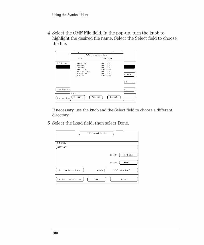
Using the Symbol Utility
4 Select the OMF File field. In the pop-up, turn the knob to highlight the desired file name. Select the Select field to choose the file.
If necessary, use the knob and the Select field to choose a different directory.
5 Select the Load field, then select Done.
580
Using the Symbol Utility
The symbol file is loaded into the analyzer. You can load several symbol files into the analyzer.
When you load a symbol file, a database file is created by the logic analyzer. Database files have an extension ".ns". If your OMF file was loaded from the hard disk drive, the database file will appear in the same subdirectory as your OMF file. If your OMF file was loaded from the flexible disk drive, the database file will appear on the hard disk drive in the same directory it was in on the flexible disk. The logic analyzer creates any necessary subdirectories on the hard disk.
See Also "To Access the Symbol File Load Menu" on page 571.
581
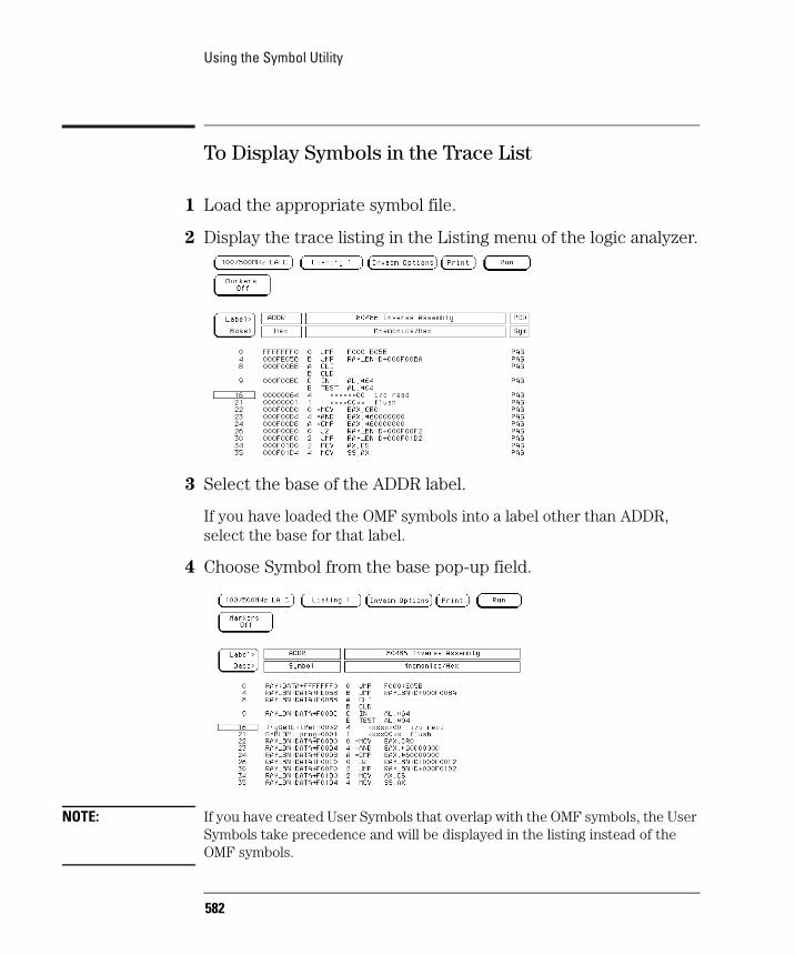
Using the Symbol Utility
To Display Symbols in the Trace List
1 Load the appropriate symbol file.
2 Display the trace listing in the Listing menu of the logic analyzer.
3 Select the base of the ADDR label.
If you have loaded the OMF symbols into a label other than ADDR, select the base for that label.
4 Choose Symbol from the base pop-up field.
NOTE: If you have created User Symbols that overlap with the OMF symbols, the User Symbols take precedence and will be displayed in the listing instead of the OMF symbols.
582
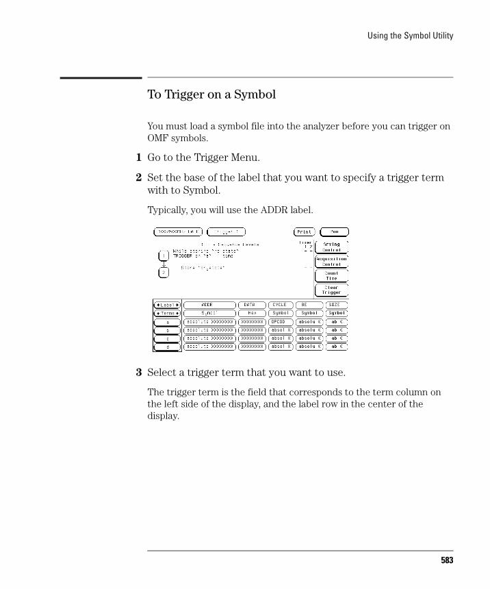
Using the Symbol Utility
To Trigger on a Symbol
You must load a symbol file into the analyzer before you can trigger on OMF symbols.
1 Go to the Trigger Menu.
2 Set the base of the label that you want to specify a trigger term with to Symbol.
Typically, you will use the ADDR label.
3 Select a trigger term that you want to use.
The trigger term is the field that corresponds to the term column on the left side of the display, and the label row in the center of the display.
583

Using the Symbol Utility
4 In the pop-up menu, select the User Symbol Table field. Choose OMF Symbol Table.
5 Use the knob to scroll through the list of symbols and pick the one that you want. Select Done.
The trigger term is now defined as one of your OMF symbols.
6 Use the symbol term in the trigger specification to trigger the logic analyzer.
584

Using the Symbol Utility
To View a List of Symbol Files Currently Loaded into the System
1 Access the OMF Symbol Load menu.
There are two methods available to access this menu. See "To Access the Symbol File Load Menu" on page 571 for more information.
2 Select the Current Loaded Files field, in the bottom left corner of the display.
A list of the symbol files that are currently loaded is displayed.
3 Select Done to return to the OMF Symbol Table menu.
585
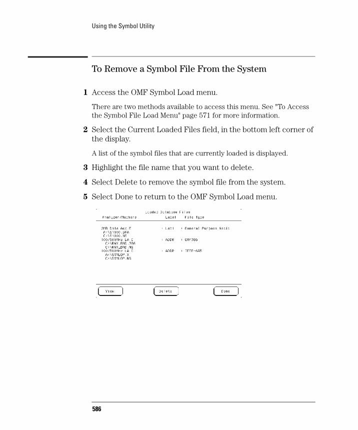
Using the Symbol Utility
To Remove a Symbol File From the System
1 Access the OMF Symbol Load menu.
There are two methods available to access this menu. See "To Access the Symbol File Load Menu" page 571 for more information.
2 Select the Current Loaded Files field, in the bottom left corner of the display.
A list of the symbol files that are currently loaded is displayed.
3 Highlight the file name that you want to delete.
4 Select Delete to remove the symbol file from the system.
5 Select Done to return to the OMF Symbol Load menu.
586

26
Symbol Utility Features and Functions
587
Symbol Utility Features and FunctionsSymbol Utility Features and Functions
Symbol Utility Features and FunctionsThe Symbol Utility adds two main menus to your logic analyzer. They are the Symbol File Load menu and the Symbol Browser menu. This chapter describes the features and functions of both of these menus.
The symbol utility also provides a General-Purpose ASCII (GPA) symbol file format that you can use if your language tool chain does not produce OMF files in one of the supported formats. The details of the GPA file format are also described in this chapter.
See Also The Logic Analyzer Training Kit for information on how to use the logic analyzer interface.
The Logic Analyzer section of this book for information on the features and functions of the logic analyzer.
588

Symbol Utility Features and FunctionsThe OMF Symbol File Load Menu
The OMF Symbol File Load MenuThe OMF Symbol Load menu is used to load the OMF files containing the symbols that you want into the logic analyzer.
OMF Symbol File Load Menu
589
Symbol Utility Features and FunctionsThe OMF Symbol File Load Menu
OMF File Field
The OMF File field is used to select the OMF file that you would like to load into the system. When you initially access the OMF Symbol Table menu, the OMF File field will be blank. To use this field, select it. A File Selection pop-up menu appears. The pop-up menu shows you a list of files at the root of the drive that is currently selected in the Drive field. Scroll the list of files to select the symbol file that you want to use. Use the Select field to choose the file, or to choose a subdirectory to browse through. Select Cancel to close the menu.
Refresh Field
The Refresh field causes the Symbol Utility to reread the contents of the disk drive. Changes made to the disk drive contents are not immediately read by the symbol utility. Use the Refresh key to re-read the disk drive contents if they have changed.
Drive Field
Use this field to specify the disk drive that contains the OMF file that you want to load. You can specify "Hard Disk" for the analyzer hard disk drive, or "Flexible Disk" for the analyzer flexible disk drive.
590
Symbol Utility Features and FunctionsThe OMF Symbol File Load Menu
Label Field
Use this field to specify the data label that the symbols will correspond to. In most cases you will use the ADDR label, since you will be loading symbols into the system that correspond to the address bits of the processor that you are working with. If you would like to load symbols that correspond to another label, select this field then choose the label that you want to use from the pop-up menu.
Module Field
This field is always Analyzer. Once the symbol file is loaded, you will be able to view the symbols in the Listing and Trigger menus.
591
Symbol Utility Features and FunctionsThe OMF Symbol File Load Menu
Load Field
Select this field to load the symbol file into the logic analyzer. During the load process, a symbol database file with a ".ns" extension will be created by the Symbol Utility. You can load multiple symbol databases into the system at the same time. One .ns database file will be created for each symbol file that you load.
If the OMF symbol file is loaded from the hard disk drive, the .ns database file will be created on the same subdirectory that the OMF file is in. If the OMF file is loaded from the flexible disk drive, the directory path from the flexible disk drive will be duplicated on the hard disk drive. The .ns database file will be created on the hard disk drive, in the same subdirectory that the OMF file was in on the flexible disk drive.
Once the .ns file is created, the Symbol Utility will use this file as its working symbol database. The next time you need to load the symbols into the system, you can load the .ns file explicitly, by placing the .ns file name in the "OMF file" field. You can purge the OMF file from the disk, once the .ns file is created.
OMF file versions
If you load an OMF file that has been loaded previously, the system will compare the time stamps on the .ns file and the OMF file. If the OMF file is newer than the existing .ns file, a new .ns file will be created and the old one will be overwritten. If the OMF file being loaded has not been updated since it was last loaded, the existing .ns file will be used.
Multiple files
You can load multiple symbol files into the analyzer. Symbols from each of the files that you load will appear in the OMF Symbol Browser menu and can be used to create trigger terms for the logic analyzer.
592
Symbol Utility Features and FunctionsThe OMF Symbol File Load Menu
Current Loaded Files Field
Select this field to view a list of the symbol files that are currently loaded. The Loaded Database Files pop-up menu provides a Delete field that you can use to remove a symbol database. Use the knob to highlight the symbol file that you want to remove. Select the Delete field to remove the file.
View Field
The View field is used to select the database that you want to be work with in the OMF Symbol Table load menu. If more than one database has been loaded, you can choose the database that you want to work with by highlighting the analyzer and file name and selecting the View field.
The file name that you select will appear in the OMF File field in the main OMF Symbol Table load menu. You can now change the file characteristics, such as the Section Relocation options.
593
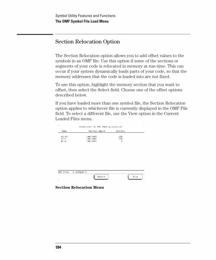
Symbol Utility Features and FunctionsThe OMF Symbol File Load Menu
Section Relocation Option
The Section Relocation option allows you to add offset values to the symbols in an OMF file. Use this option if some of the sections or segments of your code is relocated in memory at run-time. This can occur if your system dynamically loads parts of your code, so that the memory addresses that the code is loaded into are not fixed.
To use this option, highlight the memory section that you want to offset, then select the Select field. Choose one of the offset options described below.
If you have loaded more than one symbol file, the Section Relocation option applies to whichever file is currently displayed in the OMF File field. To select a different file, use the View option in the Current Loaded Files menu.
Section Relocation Menu
594
Symbol Utility Features and FunctionsThe OMF Symbol File Load Menu
Set Absolute Section Location
Use this option to set an absolute address for the start of the selected section, when you know the run-time address of the section.
Offset This Section
Use this option to add an offset to the start of the selected section, when you know the relocation offset of the section. The value entered will be added to the section address that was contained in the OMF file. All symbols falling within the address range of this section will be offset by this value.
Offset All Sections
This option adds an offset to the starting addresses of all sections in the selected OMF file. The values entered will be added to all relocatable sections in your program. You will typically use this option if you have PC relative code and data.
A section that contains symbols for hardware addresses will usually be indicated as nonrelocatable in the OMF file. The symbols for these sections will not be relocated.
595
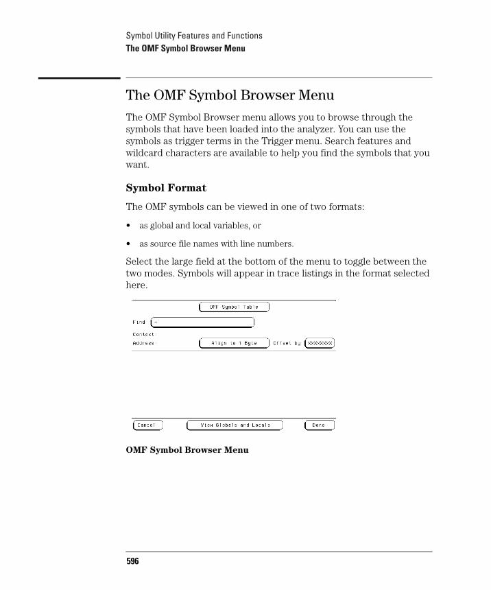
Symbol Utility Features and FunctionsThe OMF Symbol Browser Menu
The OMF Symbol Browser MenuThe OMF Symbol Browser menu allows you to browse through the symbols that have been loaded into the analyzer. You can use the symbols as trigger terms in the Trigger menu. Search features and wildcard characters are available to help you find the symbols that you want.
Symbol Format
The OMF symbols can be viewed in one of two formats:
• as global and local variables, or
• as source file names with line numbers.
Select the large field at the bottom of the menu to toggle between the two modes. Symbols will appear in trace listings in the format selected here.
OMF Symbol Browser Menu
596

Symbol Utility Features and FunctionsThe OMF Symbol Browser Menu
Symbol Type Selection Field (User vs. OMF)
This field allows you to choose between the two types of symbols available in the logic analyzer. The choices are:
• "User Symbols," corresponding to the symbols that you can define in the Format menu, and
• "OMF Symbols," corresponding to the symbols in an OMF symbol file that you have loaded using the Symbol Utility.
This field appears at the top of the pop-up menu, when you select a trigger term.
Symbol Type Selection Pop-up
597

Symbol Utility Features and FunctionsThe OMF Symbol Browser Menu
Find Field
Use this field to locate particular symbols in the symbol databases that you would like to use in a trigger specification. When you first access the OMF Symbol Table menu, the Find field will display an asterisk (*). The asterisk is a wildcard character that you can use in browsing the symbol database for the symbol that you want. To begin using this field, select it, type in the name of a file or symbol, then select Done. When you type in a symbol name and select Done, the system searches the symbol database for symbols that match this name.
Asterisk wildcard (*)
The asterisk wildcard represents "any characters." When you perform a search on the symbol database using just the asterisk, you will see a list of all symbols contained in the database. The asterisk can also be added to a search word to find all symbols that begin or end with the same letters.
Example To find all of the symbols that begin with the letters "st", select the Find field and type "st*". Select Done and the browse results look like this:
Highlight the symbol that you want and select Done to use the symbol as a trigger term.
598
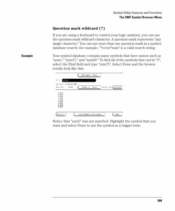
Symbol Utility Features and FunctionsThe OMF Symbol Browser Menu
Question mark wildcard (?)
If you are using a keyboard to control your logic analyzer, you can use the question mark wildcard character. A question mark represents "any single character." You can use more than one question mark in a symbol database search; for example, "?ector?num" is a valid search string.
Example Your symbol database contains many symbols that have names such as "sym1," "sym17," and "sym20." To find all of the symbols that end in "5", select the Find field and type "sym?5". Select Done and the browse results look like this:
Notice that "sym5" was not matched. Highlight the symbol that you want and select Done to use the symbol as a trigger term.
599

Symbol Utility Features and FunctionsThe OMF Symbol Browser Menu
Browse Results Display
This area of the display shows you a list of the symbols that satisfy the search criteria that you have specified. Depending on the mode selected in the large field at the bottom of the display, the browse results display will show file names and line numbers, or the symbol names. The field can be scrolled to view additional symbols that are offscreen.
Scroll Files field
This field appears if the symbol mode field, at the bottom of the screen, is set to "View Files and Line Numbers." Select this field to scroll the listing of the browse results. If this field is not selected, then the Line Number field can be scrolled.
600
Symbol Utility Features and FunctionsThe OMF Symbol Browser Menu
Align to xx Byte Option
Most processors do not fetch instructions from memory on byte boundaries. In order to trigger a logic analyzer on a symbol at an odd-numbered address, the address must be masked off. The "Align to Byte" option allows you to mask off an address.
Example The symbol "main" occurs at address 100F. The processor being probed is a 68040, which fetches instructions on long word (4-byte) boundaries. In order to trigger on the address 100F, the address must be masked off to the nearest 4-byte boundary. The Align to Byte option would be set to "Align to 4 bytes." The Symbol Utility masks the address of the symbol "main" to 100C hex before it is used as a trigger term.
601

Symbol Utility Features and FunctionsThe OMF Symbol Browser Menu
Offset Option
The Offset option allows you to add an offset value to the starting point of the symbol that you want to use as a trigger term. You might do this in order to trigger on a point in a function that is beyond the preamble of the function, or to trigger on a point that is past the prefetch depth of the processor. Setting an offset helps to avoid false triggers in these situations.
The offset specified in the Offset field is applied before the address masking is done by the "Align to xx Byte" option.
Example An 80386 processor has a prefetch depth of 16 bytes. Functions func1 and func2 are adjacent to each other in physical memory, with func2 following func1. In order to trigger on func2, without getting a false trigger from a prefetch beyond the end of func1, you need to add an offset value that is equal to or greater than the prefetch depth of the processor to your trigger term. In this case you want to add an offset of 16 bytes, so you would set the value of the "Offset by" field to 10 hex. When you specify func2 as your trigger term, the logic analyzer will trigger on address func2+10.
602
Symbol Utility Features and FunctionsThe OMF Symbol Browser Menu
Context Display
The Context display, just below the Find field, indicates the original OMF source file for the symbol that is currently highlighted in the Browse Results display. A: indicates the flexible disk drive. C: indicates the hard disk drive.
Some OMF formats, such as IEEE-695, provide information about the path name of the original source files. If you are using one of these OMF formats, you will see path information for the individual files in the browse results display. The source file path name is separated from the OMF path by a colon (:).
Example An OMF file called symlop.x has been loaded from the hard disk drive of the Agilent Technologies 16500B. One of the source files for the OMF was called main.c. When you browse symbols from the symbol database, the context display might look like this:
Context: C:\symlop.x:/users/fred/project/src/main.c
C:\symlop.x is the path for the OMF file on the 16500B hard disk. /users/fred... is the path for the file main.c in the original environment where it was compiled.
Address Display
The Address display indicates the address corresponding to the symbol that is currently highlighted in the Browse Results display. The addresses are displayed as physical values. Intel 80x86 segment:offset values are converted to physical address values before they are displayed.
603
Symbol Utility Features and FunctionsThe OMF Symbol Browser Menu
Symbol Mode Field
The OMF symbols can be viewed in one of two formats:
• as global and local symbols, or
• as source file names with line numbers
Select the large field at the bottom of the display to toggle between the two modes. Symbols appear in the trace listing in the format that is selected here.
When the "View Globals and Locals" mode is selected, the browse results are displayed as symbolic names. When the "View Files and Line Numbers" mode is selected, the browse results display lists source file names from the OMF file. In the "View Files and Line Numbers" mode, two additional fields appear in the OMF Symbol Browser menu.
The Scroll Files Field
Select this field to assign the knob to scroll the Browse Results listing.
Line Number Field
The Line Number field is used to select a line number of a source file as a trigger term. Select the field once and it can be used to scroll through the line numbers of valid, existing lines of code. Select the field a second time and a keypad pop-up allows you to specify a particular line number.
Not all lines in a source file have code associated with them. When you type in a line number that contains no code, the field defaults to the next highest line number that does contain code. If you select a line number higher than any line number in the file, the field defaults to the highest line number in the file.
604
Symbol Utility Features and FunctionsThe General-Purpose ASCII File Format
The General-Purpose ASCII File FormatThe Symbol Utility supports a General-Purpose ASCII (GPA) file format. If your language tool chain does not produce one of the supported file types, you can create a GPA file to define symbols for the Symbol Utility. You can also use a GPA file to define symbols which are not included in a supported OMF file.
605

Symbol Utility Features and FunctionsThe General-Purpose ASCII File Format
Creating a GPA Symbol File
You can create a GPA symbol file using any text editor that supports ASCII format text. Each entry in the file you create must consist of a symbol name followed by an address or address range.
Each symbol name is a string of ASCII characters. The string can be very long, but the logic analyzer will truncate the string and use only the first 16 characters. The address or address range corresponding to a given symbol is a hexadecimal number. The address must appear immediately on the same line of the text file as the symbol name. Addresses must be separated from symbol names by one or more blank spaces or tabs. Address can be specified as a single hexadecimal value, or as a range in the following format:
beginning address..ending address
It is possible to generate a GPA file from the symbol or load map output of most language tools.
Simple Format
A GPA file can be a simple list of name/address pairs.
Example main 00001000..00001009
test 00001010..0000101F
var1 00001E22 #this is a variable
This example defines two symbols that correspond to address ranges and one point symbol that corresponds to a single address.
606
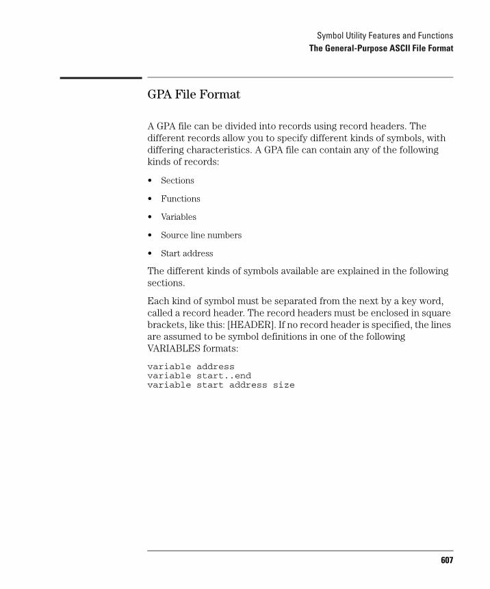
Symbol Utility Features and FunctionsThe General-Purpose ASCII File Format
GPA File Format
A GPA file can be divided into records using record headers. The different records allow you to specify different kinds of symbols, with differing characteristics. A GPA file can contain any of the following kinds of records:
• Sections
• Functions
• Variables
• Source line numbers
• Start address
The different kinds of symbols available are explained in the following sections.
Each kind of symbol must be separated from the next by a key word, called a record header. The record headers must be enclosed in square brackets, like this: [HEADER]. If no record header is specified, the lines are assumed to be symbol definitions in one of the following VARIABLES formats:
variable addressvariable start..endvariable start address size
607
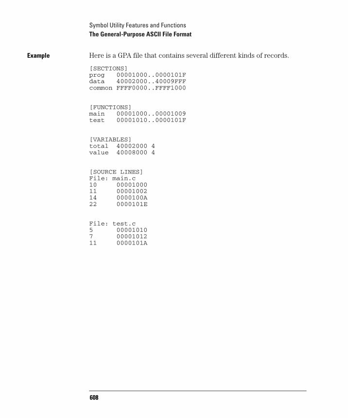
Symbol Utility Features and FunctionsThe General-Purpose ASCII File Format
Example Here is a GPA file that contains several different kinds of records.
[SECTIONS]prog 00001000..0000101Fdata 40002000..40009FFFcommon FFFF0000..FFFF1000
[FUNCTIONS]main 00001000..00001009test 00001010..0000101F
[VARIABLES]total 40002000 4value 40008000 4
[SOURCE LINES]File: main.c10 0000100011 0000100214 0000100A22 0000101E
File: test.c5 000010107 0000101211 0000101A
608
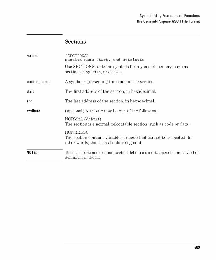
Symbol Utility Features and FunctionsThe General-Purpose ASCII File Format
Sections
Format [SECTIONS]section_name start..end attribute
Use SECTIONS to define symbols for regions of memory, such as sections, segments, or classes.
section_name A symbol representing the name of the section.
start The first address of the section, in hexadecimal.
end The last address of the section, in hexadecimal.
attribute (optional) Attribute may be one of the following:
NORMAL (default)The section is a normal, relocatable section, such as code or data.
NONRELOCThe section contains variables or code that cannot be relocated. In other words, this is an absolute segment.
NOTE: To enable section relocation, section definitions must appear before any other definitions in the file.
609

Symbol Utility Features and FunctionsThe General-Purpose ASCII File Format
Example [SECTIONS]prog 00001000..00001FFFdata 00002000..00003FFFdisplay_io 00008000..0000801F NONRELOC
NOTE: If you use section definitions in a GPA symbol file, any subsequent function or variable definitions must fall within the address ranges of one of the defined sections. Those functions and variables that do not will be ignored by the Symbol Utility.
610
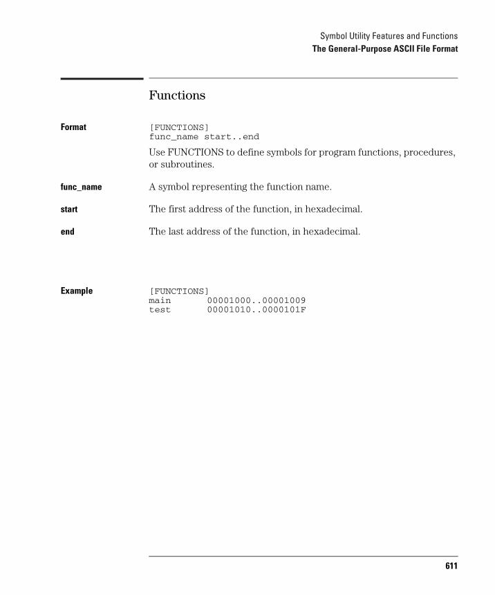
Symbol Utility Features and FunctionsThe General-Purpose ASCII File Format
Functions
Format [FUNCTIONS]func_name start..end
Use FUNCTIONS to define symbols for program functions, procedures, or subroutines.
func_name A symbol representing the function name.
start The first address of the function, in hexadecimal.
end The last address of the function, in hexadecimal.
Example [FUNCTIONS]main 00001000..00001009test 00001010..0000101F
611
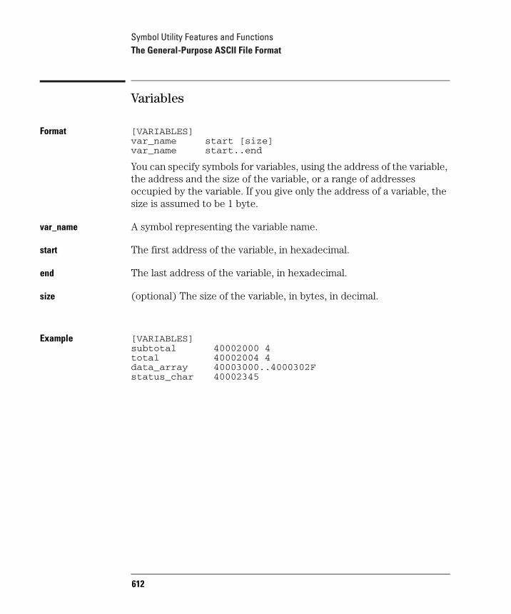
Symbol Utility Features and FunctionsThe General-Purpose ASCII File Format
Variables
Format [VARIABLES]var_name start [size]var_name start..end
You can specify symbols for variables, using the address of the variable, the address and the size of the variable, or a range of addresses occupied by the variable. If you give only the address of a variable, the size is assumed to be 1 byte.
var_name A symbol representing the variable name.
start The first address of the variable, in hexadecimal.
end The last address of the variable, in hexadecimal.
size (optional) The size of the variable, in bytes, in decimal.
Example [VARIABLES]subtotal 40002000 4total 40002004 4data_array 40003000..4000302Fstatus_char 40002345
612
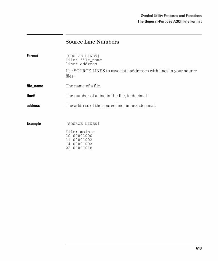
Symbol Utility Features and FunctionsThe General-Purpose ASCII File Format
Source Line Numbers
Format [SOURCE LINES]File: file_nameline# address
Use SOURCE LINES to associate addresses with lines in your source files.
file_name The name of a file.
line# The number of a line in the file, in decimal.
address The address of the source line, in hexadecimal.
Example [SOURCE LINES]
File: main.c10 0000100011 0000100214 0000100A22 0000101E
613
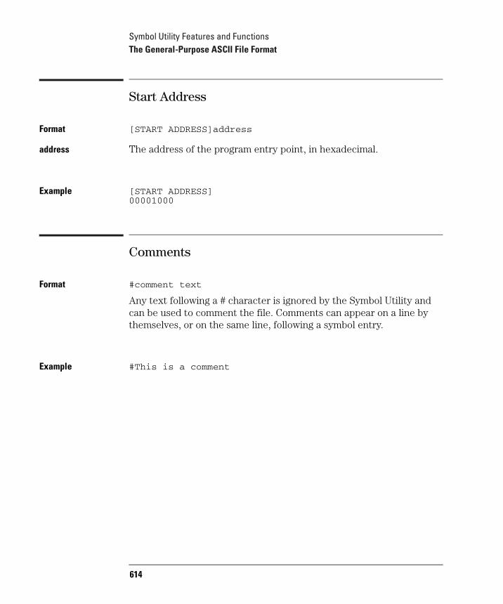
Symbol Utility Features and FunctionsThe General-Purpose ASCII File Format
Start Address
Format [START ADDRESS]address
address The address of the program entry point, in hexadecimal.
Example [START ADDRESS]00001000
Comments
Format #comment text
Any text following a # character is ignored by the Symbol Utility and can be used to comment the file. Comments can appear on a line by themselves, or on the same line, following a symbol entry.
Example #This is a comment
614
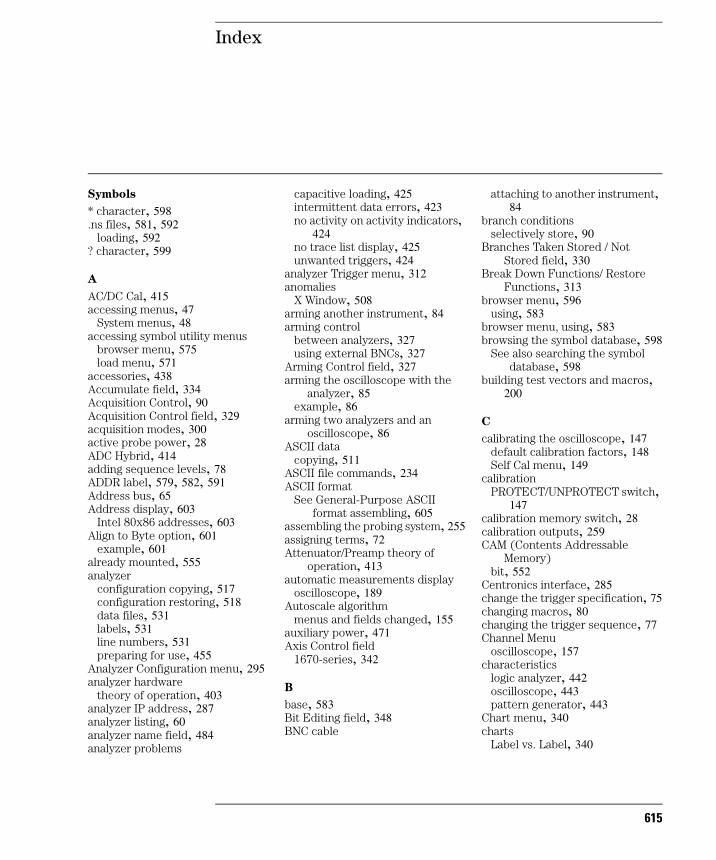
Index
Symbols
* character, 598.ns files, 581, 592
loading, 592? character, 599
A
AC/DC Cal, 415accessing menus, 47
System menus, 48accessing symbol utility menus
browser menu, 575load menu, 571
accessories, 438Accumulate field, 334Acquisition Control, 90Acquisition Control field, 329acquisition modes, 300active probe power, 28ADC Hybrid, 414adding sequence levels, 78ADDR label, 579, 582, 591Address bus, 65Address display, 603
Intel 80x86 addresses, 603Align to Byte option, 601
example, 601already mounted, 555analyzer
configuration copying, 517configuration restoring, 518data files, 531labels, 531line numbers, 531preparing for use, 455
Analyzer Configuration menu, 295analyzer hardware
theory of operation, 403analyzer IP address, 287analyzer listing, 60analyzer name field, 484analyzer problems
capacitive loading, 425intermittent data errors, 423no activity on activity indicators,
424no trace list display, 425unwanted triggers, 424
analyzer Trigger menu, 312anomalies
X Window, 508arming another instrument, 84arming control
between analyzers, 327using external BNCs, 327
Arming Control field, 327arming the oscilloscope with the
analyzer, 85example, 86
arming two analyzers and an oscilloscope, 86
ASCII datacopying, 511
ASCII file commands, 234ASCII format
See General-Purpose ASCII format assembling, 605
assembling the probing system, 255assigning terms, 72Attenuator/Preamp theory of
operation, 413automatic measurements display
oscilloscope, 189Autoscale algorithm
menus and fields changed, 155auxiliary power, 471Axis Control field
1670-series, 342
B
base, 583Bit Editing field, 348BNC cable
attaching to another instrument, 84
branch conditionsselectively store, 90
Branches Taken Stored / Not Stored field, 330
Break Down Functions/ Restore Functions, 313
browser menu, 596using, 583
browser menu, using, 583browsing the symbol database, 598
See also searching the symbol database, 598
building test vectors and macros, 200
C
calibrating the oscilloscope, 147default calibration factors, 148Self Cal menu, 149
calibrationPROTECT/UNPROTECT switch,
147calibration memory switch, 28calibration outputs, 259CAM (Contents Addressable
Memory)bit, 552
Centronics interface, 285change the trigger specification, 75changing macros, 80changing the trigger sequence, 77Channel Menu
oscilloscope, 157characteristics
logic analyzer, 442oscilloscope, 443pattern generator, 443
Chart menu, 340charts
Label vs. Label, 340
615
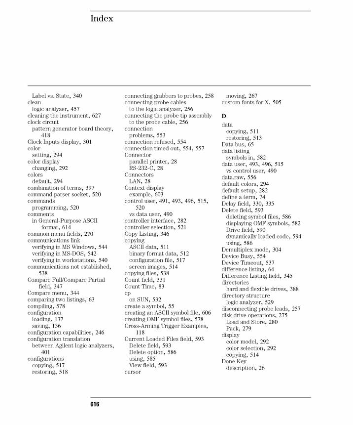
Index
Label vs. State, 340clean
logic analyzer, 457cleaning the instrument, 627clock circuit
pattern generator board theory, 418
Clock Inputs display, 301color
setting, 294color display
changing, 292colors
default, 294combination of terms, 397command parser socket, 520commands
programming, 520comments
in General-Purpose ASCII format, 614
common menu fields, 270communications link
verifying in MS Windows, 544verifying in MS-DOS, 542verifying in workstations, 540
communications not established, 538
Compare Full/Compare Partial field, 347
Compare menu, 344comparing two listings, 63compiling, 578configuration
loading, 137saving, 136
configuration capabilities, 246configuration translation
between Agilent logic analyzers, 401
configurationscopying, 517restoring, 518
616
connecting grabbers to probes, 258connecting probe cables
to the logic analyzer, 256connecting the probe tip assembly
to the probe cable, 256connection
problems, 553connection refused, 554connection timed out, 554, 557Connector
parallel printer, 28RS-232-C, 28
ConnectorsLAN, 28
Context displayexample, 603
control user, 491, 493, 496, 515, 520
vs data user, 490controller interface, 282controller selection, 521Copy Listing, 346copying
ASCII data, 511binary format data, 512configuration file, 517screen images, 514
copying files, 538Count field, 331Count Time, 83cp
on SUN, 532create a symbol, 55creating an ASCII symbol file, 606creating OMF symbol files, 578Cross-Arming Trigger Examples,
118Current Loaded Files field, 593
Delete field, 593Delete option, 586using, 585View field, 593
cursor
moving, 267custom fonts for X, 505
D
datacopying, 511restoring, 513
Data bus, 65data listing
symbols in, 582data user, 493, 496, 515
vs control user, 490data.raw, 556default colors, 294default setup, 282define a term, 74Delay field, 330, 335Delete field, 593
deleting symbol files, 586displaying OMF symbols, 582Drive field, 590dynamically loaded code, 594using, 586
Demultiplex mode, 304Device Busy, 554Device Timeout, 537difference listing, 64Difference Listing field, 345directories
hard and flexible drives, 388directory structure
logic analyzer, 529disconnecting probe leads, 257disk drive operations, 275
Load and Store, 280Pack, 279
displaycolor model, 292color selection, 292copying, 514
Done Keydescription, 26
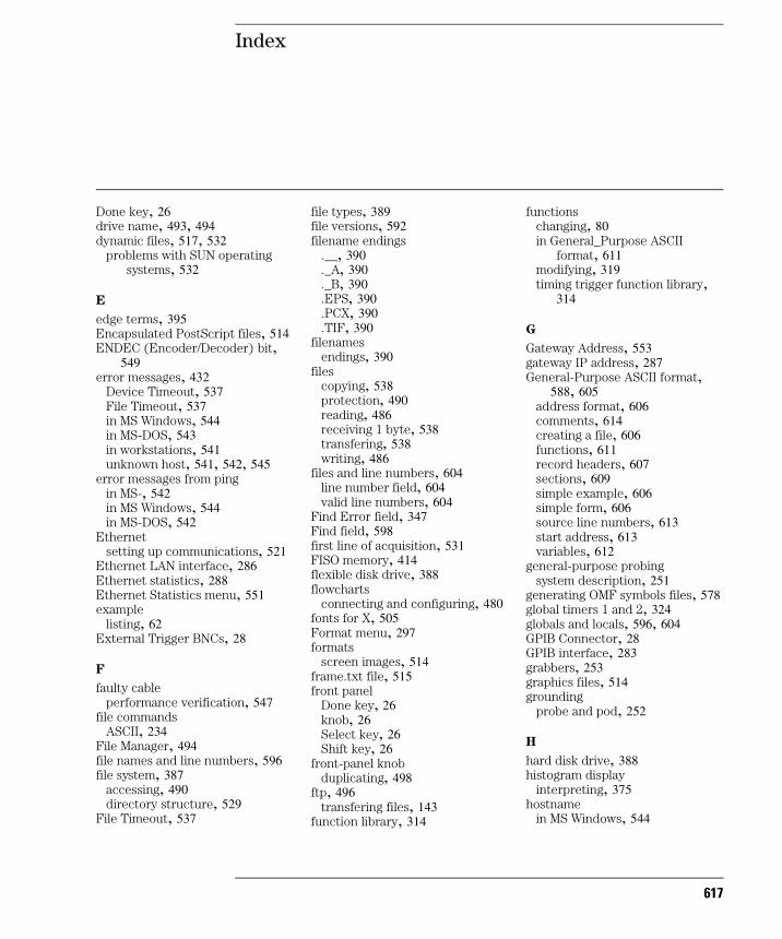
Index
Done key, 26drive name, 493, 494dynamic files, 517, 532
problems with SUN operating systems, 532
E
edge terms, 395Encapsulated PostScript files, 514ENDEC (Encoder/Decoder) bit,
549error messages, 432
Device Timeout, 537File Timeout, 537in MS Windows, 544in MS-DOS, 543in workstations, 541unknown host, 541, 542, 545
error messages from pingin MS-, 542in MS Windows, 544in MS-DOS, 542
Ethernetsetting up communications, 521
Ethernet LAN interface, 286Ethernet statistics, 288Ethernet Statistics menu, 551example
listing, 62External Trigger BNCs, 28
F
faulty cableperformance verification, 547
file commandsASCII, 234
File Manager, 494file names and line numbers, 596file system, 387
accessing, 490directory structure, 529
File Timeout, 537
file types, 389file versions, 592filename endings
.__, 390
._A, 390
._B, 390
.EPS, 390
.PCX, 390
.TIF, 390filenames
endings, 390files
copying, 538protection, 490reading, 486receiving 1 byte, 538transfering, 538writing, 486
files and line numbers, 604line number field, 604valid line numbers, 604
Find Error field, 347Find field, 598first line of acquisition, 531FISO memory, 414flexible disk drive, 388flowcharts
connecting and configuring, 480fonts for X, 505Format menu, 297formats
screen images, 514frame.txt file, 515front panel
Done key, 26knob, 26Select key, 26Shift key, 26
front-panel knobduplicating, 498
ftp, 496transfering files, 143
function library, 314
functionschanging, 80in General_Purpose ASCII
format, 611modifying, 319timing trigger function library,
314
G
Gateway Address, 553gateway IP address, 287General-Purpose ASCII format,
588, 605address format, 606comments, 614creating a file, 606functions, 611record headers, 607sections, 609simple example, 606simple form, 606source line numbers, 613start address, 613variables, 612
general-purpose probingsystem description, 251
generating OMF symbols files, 578global timers 1 and 2, 324globals and locals, 596, 604GPIB Connector, 28GPIB interface, 283grabbers, 253graphics files, 514grounding
probe and pod, 252
H
hard disk drive, 388histogram display
interpreting, 375hostname
in MS Windows, 544
617
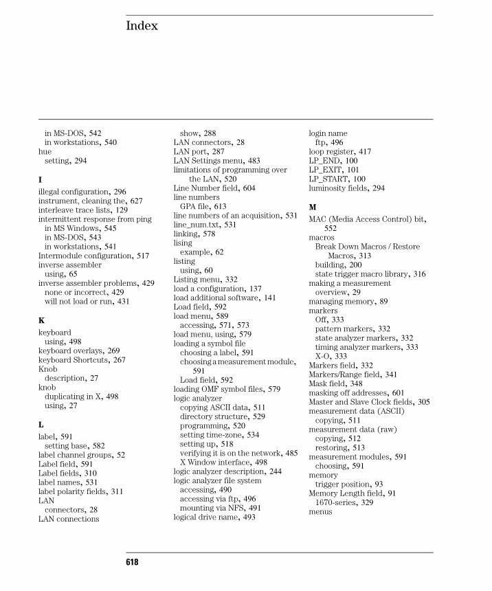
Index
in MS-DOS, 542in workstations, 540
huesetting, 294
I
illegal configuration, 296instrument, cleaning the, 627interleave trace lists, 129intermittent response from ping
in MS Windows, 545in MS-DOS, 543in workstations, 541
Intermodule configuration, 517inverse assembler
using, 65inverse assembler problems, 429
none or incorrect, 429will not load or run, 431
K
keyboardusing, 498
keyboard overlays, 269keyboard Shortcuts, 267Knob
description, 27knob
duplicating in X, 498using, 27
L
label, 591setting base, 582
label channel groups, 52Label field, 591Label fields, 310label names, 531label polarity fields, 311LAN
connectors, 28LAN connections
618
show, 288LAN connectors, 28LAN port, 287LAN Settings menu, 483limitations of programming over
the LAN, 520Line Number field, 604line numbers
GPA file, 613line numbers of an acquisition, 531line_num.txt, 531linking, 578lising
example, 62listing
using, 60Listing menu, 332load a configuration, 137load additional software, 141Load field, 592load menu, 589
accessing, 571, 573load menu, using, 579loading a symbol file
choosing a label, 591choosing a measurement module,
591Load field, 592
loading OMF symbol files, 579logic analyzer
copying ASCII data, 511directory structure, 529programming, 520setting time-zone, 534setting up, 518verifying it is on the network, 485X Window interface, 498
logic analyzer description, 244logic analyzer file system
accessing, 490accessing via ftp, 496mounting via NFS, 491
logical drive name, 493
login nameftp, 496
loop register, 417LP_END, 100LP_EXIT, 101LP_START, 100luminosity fields, 294
M
MAC (Media Access Control) bit, 552
macrosBreak Down Macros / Restore
Macros, 313building, 200state trigger macro library, 316
making a measurementoverview, 29
managing memory, 89markers
Off, 333pattern markers, 332state analyzer markers, 332timing analyzer markers, 333X-O, 333
Markers field, 332Markers/Range field, 341Mask field, 348masking off addresses, 601Master and Slave Clock fields, 305measurement data (ASCII)
copying, 511measurement data (raw)
copying, 512restoring, 513
measurement modules, 591choosing, 591
memorytrigger position, 93
Memory Length field, 911670-series, 329
menus

Index
new, 533Min and Max scaling fields, 341mixed display
state and timing, 131Mixed Display menu, 338Modify Trigger field, 313Module field, 591module status, 515mount
control user, 486data user, 486error message, 486in UNIX, 486
mounting and unmounting, 486mouse
using, 498MS Windows
error messages from ping, 545File Manager, 494intermittent response from ping,
545mount, 487, 494no response from ping, 545ping, 485
MS-DOSerror messages, 542error messages from ping, 542hostname, 542intermittent response from ping,
543mount, 487, 493no response from ping, 543normal response from ping, 542ping, 485, 542unknown host, 542
multiple OMF files, 592multiple symbol files, 592
N
networkconfiguring the logic analyzer,
482, 484
connecting, 481mounting, 486statistics, 551
network addressesaccessing, 482configuring, 482
no heartbeat, 552no more mounts available, 555no response from ping
in MS-DOS, 543in workstations, 541
filename endings, 390
normal response from pingin MS-DOS, 542in workstations, 540
numbers, 604
O
occurrence counters, 321odd-numbered addresses, 601offset
adding to address values, 594all sections, 595code section, 595trigger term, 602
Offset All Sections option, 595Offset option of browser menu, 602
example, 602Offset This Section option, 595OMF File field, 590
Refresh field, 590using, 580
OMF Load fieldusing, 580
OMF symbol filescreating, 578currently loaded, 585deleting, 586versions, 592
OMF Symbol Tablebrowser menu, 596
browser menu, accessing, 575load menu, accessing, 571
OMF Symbol Table menus, 588OMF symbols
browsing, 575, 598loading into logic analyzer, 571,
579symbol type, 597
operating environment, 452, 455operation timed out, 557Operation Timeout, 537operator’s service, 453oscilloscope
Accumulate mode, 161automatic measurement
algorithms, 191automatic measurements
display, 189automatic time markers, 179Autoscale, 154Autoscale run, 152Auto-Trig field, 171Average mode, 160calibrating, 147channel label field, 187Channel Menu, 157Connect Dots field, 162Count field, 170, 175Coupling field, 158coupling field selections, 158Delay field, 156Display Marker Values, 163Display Options field, 163Display Sample Period, 163Displaying the waveform, 155edge trigger mode, 165Grid field, 162immediate trigger mode, 166manual time markers, 176manual/automatic time markers,
184Mode field, 160Mode/Arm menu, 164
619
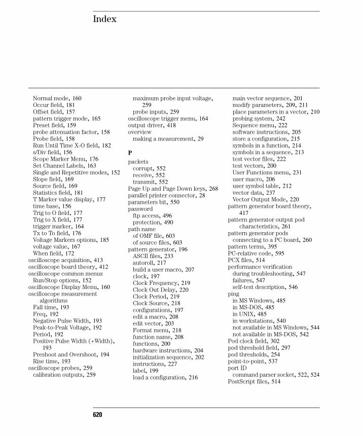
Index
Normal mode, 160Occur field, 181Offset field, 157pattern trigger mode, 165Preset field, 159probe attenuation factor, 158Probe field, 158Run Until Time X-O field, 182s/Div field, 156Scope Marker Menu, 176Set Channel Labels, 163Single and Repetitive modes, 152Slope field, 169Source field, 169Statistics field, 181T Marker value display, 177time base, 156Trig to O field, 177Trig to X field, 177trigger marker, 164Tx to To field, 176Voltage Markers options, 185voltage value, 167When field, 172
oscilloscope acquisition, 413oscilloscope board theory, 412oscilloscope common menus
Run/Stop options, 152oscilloscope Display Menu, 160oscilloscope measurement
algorithmsFall time, 193Freq, 192Negative Pulse Width, 193Peak-to-Peak Voltage, 192Period, 192Positive Pulse Width (+Width),
193Preshoot and Overshoot, 194Rise time, 193
oscilloscope probes, 259calibration outputs, 259
620
maximum probe input voltage, 259
probe inputs, 259oscilloscope trigger menu, 164output driver, 418overview
making a measurement, 29
P
packetscorrupt, 552receive, 552transmit, 552
Page Up and Page Down keys, 268parallel printer connector, 28parameters bit, 550password
ftp access, 496protection, 490
path nameof OMF file, 603of source files, 603
pattern generator, 196ASCII files, 233autoroll, 217build a user macro, 207clock, 197Clock Frequency, 219Clock Out Delay, 220Clock Period, 219Clock Source, 218configurations, 197edit a macro, 208edit vector, 203Format menu, 218function name, 208functions, 200hardware instructions, 204initialization sequence, 202instructions, 227label, 199load a configuration, 216
main vector sequence, 201modify parameters, 209, 211place parameters in a vector, 210probing system, 242Sequence menu, 222software instructions, 205store a configuration, 215symbols in a function, 214symbols in a sequence, 213test vector files, 222test vectors, 200User Functions menu, 231user macro, 206user symbol table, 212vector data, 237Vector Output Mode, 220
pattern generator board theory, 417
pattern generator output pod characteristics, 261
pattern generator podsconnecting to a PC board, 260
pattern terms, 395PC-relative code, 595PCX files, 514performance verification
during troubleshooting, 547failures, 547self-test description, 546
pingin MS Windows, 485in MS-DOS, 485in UNIX, 485in workstations, 540not available in MS Windows, 544not available in MS-DOS, 542
Pod clock field, 302pod threshold field, 297pod thresholds, 254point-to-point, 537port ID
command parser socket, 522, 524PostScript files, 514
Index
power requirements, 455power-up tests, 461prefetch, 601
offsetting trigger term, 602preprocessor problems, 426
erratic trace measurements, 428slow clock, 427target system boot up failure, 426
Print All, 272Print Disk, 272Print field, 271Print Partial, 272Print Screen, 271printer interface, 282probe and pod grounding, 252probe cable, 253probe leads, 252probe tip assemblies, 251probing, 248
assembling the probing system, 255
connecting grabbers to probes, 258
general-purpose, 249grabbers, 253maximum probe input voltage,
254microprocessor and bus-specific
interfaces, 249minimum signal amplitude, 253oscilloscope probes, 259pattern generator output pod
characteristics, 261pod thresholds, 254probe cable, 253termination adapter, 250
programmingsetting up, 521
PROTECT/UNPROTECT switch, 147
R
RAMpattern generator board theory,
418range terms, 395raw measurement data
copying, 512restoring, 513
reading files, 486reading statistics, 551read-only access to file system, 490read-write access to file system,
490Real Time Clock Adjustments field,
289real-time limitations, 520receive an arm signal
from another instrument, 87receive packets, 552record headers, 607Reference Listing field, 345Refresh field, 590relative trigger time, 515relocation of code, 594removing symbol files, 586Repetitive, 273Rescale field, 343Resource terms, 323return to Agilent service, 559Roll fields, 274RS-232-C interface, 284RS-232-C, GPIB, and Centronics
Interfaces, 282Run/Stop field, 273Rx bit, 550
S
sampling rates, 94Saturation
setting, 294save a configuration, 136
save a trace list in ASCII format, 139
Scope Auto Measure menu, 188screen images, 514Scroll Files field, 600, 604searching the symbol database, 598
results, 600sec/Div field, 334Section Relocation Option, 594
Offset All Sections option, 595Offset This Section option, 595Set Absolute Section Location
option, 595sections
in General-Purpose ASCII format, 609
Select Keydescription, 26
Select key, 26self-tests, 462Self-tests description, 420sequence levels, 392
adding, 78server not responding, 554service
return to Agilent, 559Set Absolute Section Location
option, 595set the memory length, 91set up time correlation
between a timing and a state analyzer, 83
between two state analyzers, 82setting
color, 294hue, 294saturation, 294
setting the manual/automatic time markers
oscilloscope, 184setup.raw, 556setup.raw files
copying, 517
621
Index
restoring, 518Setup/Hold field, 307Shift Key
description, 27Shift key, 27single-client/single-server, 537,
543, 545size of files, 532slow operation, 557socket, 520
command parser, 524port ID number, 522, 524
source line numbersin General-Purpose ASCII
format, 613SPA (System Performance
Analysis)changing between SPA and the
analyzer, 383programming, 383using in Group Runs, 384using with other features, 383
special displaysinterleaved trace lists, 128Mixed Display mode, 128
specifications, 437logic analyzer, 440oscilloscope, 441
stale NFS file handle, 491start address
in General-Purpose ASCII format, 613
state acquisition modes, 298state acquisitions
comparing, 63State Histogram example, 365State Histogram mode, 362
using, 376state listings
interleaving, 338State Overview mode
using, 373state tags, 531
622
state trigger function library, 316statistics markers, 333status bits, 549status information, 515status number
description, 548SUN workstations, 532supplemental characteristics
logic analyzer, 445oscilloscope, 450
support services, 559symbol
create, 55symbol base, 582symbol browser menu
accessing, 575using, 583
symbol database.ns files, 581creating, 592
symbol file load menu, 589accessing, 571using, 579
symbol format, 596choosing, 604
symbol modechoosing, 604
symbol type, 597precedence, 582
symbolsbrowsing, 598
Symbols field, 308system configuration, 517System Performance Analysis
description, 352labels, 358measurement processes, 357operating characteristics, 353sampling and sorting, 358State Histrogram mode, 354State Overview example, 361State Overview mode, 353, 359three trace modes example, 370
Time Interval example, 369Time Interval mode, 354, 366
System Performance Analysis (SPA)
getting started using, 355System Performance Analysis
(SPA) Software, 350System Utilities, 289system.txt file, 515
T
tagsTime and State, 331
termdefine, 74
termination adapter, 250termination bit, 552terms
assigning, 72assigning bit by bit, 325bit pattern terms a-j, 323changing names and values, 324combination of terms, 326edge terms 1 and 2, 324range terms 1 and 2, 323using preset values, 325
testlogic analyzer, 457
theory of operation, 404logic acquisition board, 408oscilloscope board, 412pattern generator board, 417
TIFF files, 514Time Correlation, 81Time Interval mode
using, 379time tags, 531time_abs.txt, 531time-correlated displays, 339timeout bit, 550timeout errors, 537timers, 321, 395

Index
timing acquisition modes, 299timing sampling rates, 94timing trigger function library, 314trace listing
symbols in, 582trace lists
interleave, 129trace modes (SPA), 357TRANS (Transceiver) bit, 550transfer files using ftp, 143transferring files, 538
using the flexible disk drive, 135using the LAN, 142
transmit packets, 552trigger
customizing a basic trigger, 71trigger example
nth recursive call of a recursive function, 102
trigger examplescapture a write of known bad data
to a particular variable, 106capture the waveform of a glitch,
123detect a glitch, 122detect bus contention, 117execution of a subroutine, 98expected data does not appear
when requested, 112find the nth assertion of a chip
select line, 110handshake violation, 116look at control and status signals,
121loop overrun, 107minimum and maximum pulse
limits, 114monitor two coprocessors in a
target system, 126nth iteration of a loop, 100software execution when a timing
violation occurs, 119
timing analysis of a count-down on a set of data lines, 125
trigger after lines have finished transitioning, 109
trigger on entry to a function, 104verify correct return from a
function call, 108verify the chip select line is
strobed after the address is stable, 111
view your target system processing an interrupt, 124
trigger functionschanging, 80
trigger positionstart, center, end, 93
Trigger Position field, 329trigger sequence
state analyzer, 400timing analyzer, 400
trigger sequence levels, 312trigger sequence specification, 392trigger specification
changing, 75trigger term, 583, 596triggering on a symbol, 583
browser menu, 596finding the symbol you want, 598odd-numbered addresses, 601
triggersbranching, 321
troubleshooting, 422analyzer problems, 423error messages, 432in MS Windows, 544in MS-DOS, 542in workstations, 540inverse assembler problems, 429preprocessor problems, 426
troubleshooting flowcharts, 458, 459
Tx bit, 550
U
unable to open window, 555UNIX
mount, 486, 491ping, 485
unknown host messagein MS Windows, 544in MS-DOS, 542in workstations, 540
unmount, 486Update FLASH ROM field, 290User Symbols, 582, 597
V
variableGeneral-Purpose ASCII format,
612vector
place parameters, 210vectors
building, 200versions of OS, 515versions of symbol files, 592View field, 593View Files and Line Numbers, 604
valid line numbers, 604View Globals and Locals, 604viewing OMF symbols, 582Voltage Markers options
oscilloscope, 185
W
W Window interfaceanomalies, 508
waveformusing, 57
Waveform display, 337waveform label field, 335Waveform menu, 334waveform menu, 57wildcard characters
*character, 598
623
Index
workstationserror messages, 541error messages from ping, 541hostname, 540intermittent response from ping,
541no response from ping, 541normal response from ping, 540troubleshooting in, 540
writing files, 486
X
X Window Interfaceloading custom fonts, 505
X Window interface, 498closing, 504starting, 499
624
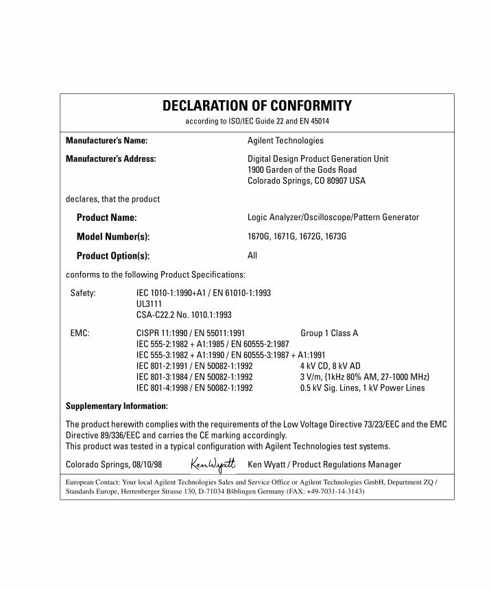
DECLARATION OF CONFORMITYaccording to ISO/IEC Guide 22 and EN 45014
Manufacturer’s Name: Agilent Technologies
Manufacturer’s Address: Digital Design Product Generation Unit1900 Garden of the Gods RoadColorado Springs, CO 80907 USA
declares, that the product
Product Name: Logic Analyzer/Oscilloscope/Pattern Generator
Model Number(s): 1670G, 1671G, 1672G, 1673G
Product Option(s): All
conforms to the following Product Specifications:
Safety: IEC 1010-1:1990+A1 / EN 61010-1:1993UL3111CSA-C22.2 No. 1010.1:1993
EMC: CISPR 11:1990 / EN 55011:1991 Group 1 Class AIEC 555-2:1982 + A1:1985 / EN 60555-2:1987IEC 555-3:1982 + A1:1990 / EN 60555-3:1987 + A1:1991IEC 801-2:1991 / EN 50082-1:1992 4 kV CD, 8 kV ADIEC 801-3:1984 / EN 50082-1:1992 3 V/m, 1kHz 80% AM, 27-1000 MHzIEC 801-4:1998 / EN 50082-1:1992 0.5 kV Sig. Lines, 1 kV Power Lines
Supplementary Information:
The product herewith complies with the requirements of the Low Voltage Directive 73/23/EEC and the EMC Directive 89/336/EEC and carries the CE marking accordingly.This product was tested in a typical configuration with Agilent Technologies test systems.
Colorado Springs, 08/10/98 Ken Wyatt / Product Regulations Manager
European Contact: Your local Agilent Technologies Sales and Service Office or Agilent Technologies GmbH, Department ZQ / Standards Europe, Herrenberger Strasse 130, D-71034 Bšblingen Germany (FAX: +49-7031-14-3143)
Product Regulations
Safety IEC 1010-1:1990+A1 / EN 61010-1:1993UL3111CSA-C22.2 No. 1010.1:1993
EMC This Product meets the requirement of the European Communities (EC) EMC Directive 89/336/EEC.
Emissions EN55011/CISPR 11 (ISM, Group 1, Class A equipment)IEC 555-2 and IEC 555-3
Immunity EN50082-1 Code1 Notes2
IEC 801-2 (ESD) 8kV ADIEC 801-3 (Rad.) 3V/mIEC 801-4 (EFT) 1kV
111
1Performance Codes:1 PASS - Normal operation, no effect.2 PASS - Temporary degradation, self recoverable.3 PASS - Temporary degradation, operator intervention required.4 FAIL - Not recoverable, component damage.
2Notes: (none)
Sound Pressure Level
Less than 60 dBA
Regulatory Information for Canada
ICES/NMB-001
This ISM device complies with Canadian ICES-001.Cet appareil ISM est confomre à la norme NMB-001 du Canada.
Regulatory Information for Australia/New Zealand
This ISM device complies with Australian/New Zealand AS/NZS 2064.1
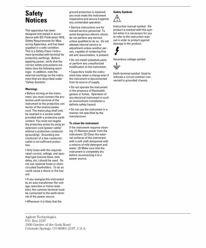
Safety NoticesThis apparatus has been designed and tested in accor-dance with IEC Publication 1010, Safety Requirements for Mea-suring Apparatus, and has been supplied in a safe condition. This is a Safety Class I instru-ment (provided with terminal for protective earthing). Before applying power, verify that the correct safety precautions are taken (see the following warn-ings). In addition, note the external markings on the instru-ment that are described under "Safety Symbols."
Warnings• Before turning on the instru-ment, you must connect the pro-tective earth terminal of the instrument to the protective con-ductor of the (mains) power cord. The mains plug shall only be inserted in a socket outlet provided with a protective earth contact. You must not negate the protective action by using an extension cord (power cable) without a protective conductor (grounding). Grounding one conductor of a two-conductor outlet is not sufficient protec-tion.
• Only fuses with the required rated current, voltage, and spec-ified type (normal blow, time delay, etc.) should be used. Do not use repaired fuses or short-circuited fuseholders. To do so could cause a shock or fire haz-ard.
• If you energize this instrument by an auto transformer (for volt-age reduction or mains isola-tion), the common terminal must be connected to the earth termi-nal of the power source.
• Whenever it is likely that the
Agilent TechnologiesP.O. Box 21971900 Garden of the Gods RoColorado Springs, CO 80901
ground protection is impaired, you must make the instrument inoperative and secure it against any unintended operation.
• Service instructions are for trained service personnel. To avoid dangerous electric shock, do not perform any service unless qualified to do so. Do not attempt internal service or adjustment unless another per-son, capable of rendering first aid and resuscitation, is present.
• Do not install substitute parts or perform any unauthorized modification to the instrument.
• Capacitors inside the instru-ment may retain a charge even if the instrument is disconnected from its source of supply.
• Do not operate the instrument in the presence of flammable gasses or fumes. Operation of any electrical instrument in such an environment constitutes a definite safety hazard.
• Do not use the instrument in a manner not specified by the manufacturer.
To clean the instrumentIf the instrument requires clean-ing: (1) Remove power from the instrument. (2) Clean the exter-nal surfaces of the instrument with a soft cloth dampened with a mixture of mild detergent and water. (3) Make sure that the instrument is completely dry before reconnecting it to a power source.
ad-2197, U.S.A.
Safety Symbols
Instruction manual symbol: the product is marked with this sym-bol when it is necessary for you to refer to the instruction man-ual in order to protect against damage to the product..
Hazardous voltage symbol.
Earth terminal symbol: Used to indicate a circuit common con-nected to grounded chassis.
!

Notices© Agilent Technologies, Inc. 2002
No part of this manual may be reproduced in any form or by any means (including electronic storage and retrieval or translation into a foreign language) without prior agreement and written consent from Agilent Technologies, Inc. as governed by United States and international copyright laws.
Manual Part Number01670-97022, August 2002
Print History01670-97020, November 200101670-97017, May 200101670-97016, January 200101670-97014, January 2000
Agilent Technologies, Inc.1900 Garden of the Gods Road Colorado Springs, CO 80907 USA
Restricted Rights LegendIf software is for use in the per-formance of a U.S. Government prime contract or subcontract, Software is delivered and licensed as “Commercial com-puter software” as defined in DFAR 252.227-7014 (June 1995), or as a “commercial item” as defined in FAR 2.101(a) or as “Restricted computer software” as defined in FAR 52.227-19 (June 1987) or any equivalent agency regulation or contract clause. Use, duplication or dis-closure of Software is subject to Agilent Technologies’ standard commercial license terms, and non-DOD Departments and Agencies of the U.S. Govern-ment will receive no greater than Restricted Rights as defined in FAR 52.227-19(c)(1-2) (June 1987). U.S. Government users will receive no greater than Limited Rights as defined in FAR 52.227-14 (June 1987) or
DFAR 252.227-7015 (b)(2) (November 1995), as applicable in any technical data.
Document WarrantyThe material contained in this document is provided “as is,” and is subject to being changed, without notice, in future editions. Further, to the maximum extent permitted by applica-ble law, Agilent disclaims all warranties, either express or implied, with regard to this manual and any information contained herein, including but not limited to the implied war-ranties of merchantability and fitness for a particular purpose. Agilent shall not be liable for errors or for inci-dental or consequential damages in connection with the furnishing, use, or per-formance of this document or of any information con-tained herein. Should Agi-lent and the user have a separate written agreement with warranty terms cover-ing the material in this docu-ment that conflict with these terms, the warranty terms in the separate agreement shall control.
Technology Licenses The hardware and/or software described in this document are furnished under a license and may be used or copied only in accordance with the terms of such license.
WARNING
A WARNING notice denotes a hazard. It calls attention to an operating procedure, practice, or the like that, if not correctly performed or adhered to, could result in personal injury or death. Do not proceed beyond a WARNING notice until the indicated conditions are fully understood and met.
CAUTION
A CAUTION notice denotes a hazard. It calls attention to an operating procedure, practice, or the like that, if not correctly performed or adhered to, could result in damage to the product or loss of important data. Do not proceed beyond a CAUTION notice until the indicated conditions are fully understood and met.
Trademark AcknowledgmentsUNIX is a registered trademark of the Open Group.