aggregate planning objective is to minimize cost over the planning period by adjusting production...

Aggregate PlanningAggregate Planning

Objective is to minimize cost over the Objective is to minimize cost over the planning period by adjustingplanning period by adjusting Production ratesProduction rates

Labor levelsLabor levels

Inventory levelsInventory levels

Overtime workOvertime work

SubcontractingSubcontracting

Other controllable variablesOther controllable variables

Determine the quantity and timing of Determine the quantity and timing of production for the immediate futureproduction for the immediate future


A logical overall unit for measuring A logical overall unit for measuring sales and outputsales and output

A forecast of demand for intermediate A forecast of demand for intermediate planning period in these aggregate unitsplanning period in these aggregate units

A method for determining costsA method for determining costs

A model that combines forecasts and A model that combines forecasts and costs so that scheduling decisions can costs so that scheduling decisions can be made for the planning periodbe made for the planning period

Required for aggregate planningRequired for aggregate planning

Master production

schedule and MRP

systems

Detailed work

schedules

Process planning and

capacity decisions

Aggregateplan for

production


Figure 13.2Figure 13.2

Product decisions

Demand forecasts,

orders

Marketplace and

demand

Researchand

technology

Raw materials available

Externalcapacity

(subcontractors)

Workforce

Inventoryon

hand


Combines appropriate resources Combines appropriate resources into general termsinto general terms

Part of a larger production planning Part of a larger production planning systemsystem

Disaggregation breaks the plan Disaggregation breaks the plan down into greater detaildown into greater detail

Disaggregation results in a master Disaggregation results in a master production scheduleproduction schedule

Aggregate Planning StrategiesAggregate Planning Strategies

1.1. Use inventories to absorb changes in Use inventories to absorb changes in demanddemand

2.2. Accommodate changes by varying Accommodate changes by varying workforce sizeworkforce size

3.3. Use part-timers, overtime, or idle time to Use part-timers, overtime, or idle time to absorb changesabsorb changes

4.4. Use subcontractors and maintain a stable Use subcontractors and maintain a stable workforceworkforce

5.5. Change prices or other factors to Change prices or other factors to influence demandinfluence demand

Capacity OptionsCapacity Options

Changing inventory levelsChanging inventory levels Increase inventory in low demand Increase inventory in low demand

periods to meet high demand in periods to meet high demand in the futurethe future

Increases costs associated with Increases costs associated with storage, insurance, handling, storage, insurance, handling, obsolescence, and capital obsolescence, and capital investmentinvestment

Shortages can mean lost sales due Shortages can mean lost sales due to long lead times and poor to long lead times and poor customer servicecustomer service


Varying workforce size by hiring Varying workforce size by hiring or layoffsor layoffs Match production rate to demandMatch production rate to demand

Training and separation costs for Training and separation costs for hiring and laying off workers hiring and laying off workers

New workers may have lower New workers may have lower productivityproductivity

Laying off workers may lower Laying off workers may lower morale and productivitymorale and productivity


Varying production rate through Varying production rate through overtime or idle timeovertime or idle time Allows constant workforceAllows constant workforce

May be difficult to meet large May be difficult to meet large increases in demandincreases in demand

Overtime can be costly and may Overtime can be costly and may drive down productivitydrive down productivity

Absorbing idle time may be Absorbing idle time may be difficultdifficult


SubcontractingSubcontracting Temporary measure during Temporary measure during

periods of peak demandperiods of peak demand

May be costlyMay be costly

Assuring quality and timely Assuring quality and timely delivery may be difficultdelivery may be difficult

Exposes your customers to a Exposes your customers to a possible competitorpossible competitor


Using part-time workersUsing part-time workers Useful for filling unskilled or low Useful for filling unskilled or low

skilled positions, especially in skilled positions, especially in servicesservices

Demand OptionsDemand Options

Influencing demandInfluencing demand Use advertising or promotion to Use advertising or promotion to

increase demand in low periodsincrease demand in low periods

Attempt to shift demand to slow Attempt to shift demand to slow periodsperiods

May not be sufficient to balance May not be sufficient to balance demand and capacitydemand and capacity


Back ordering during high- Back ordering during high- demand periodsdemand periods Requires customers to wait for an Requires customers to wait for an

order without loss of goodwill or order without loss of goodwill or the orderthe order

Most effective when there are few Most effective when there are few if any substitutes for the product if any substitutes for the product or serviceor service

Often results in lost salesOften results in lost sales


Counterseasonal product and Counterseasonal product and service mixingservice mixing Develop a product mix of Develop a product mix of

counterseasonal itemscounterseasonal items

May lead to products or services May lead to products or services outside the company’s areas of outside the company’s areas of expertiseexpertise

Aggregate Planning OptionsAggregate Planning Options

OptionOption AdvantagesAdvantages DisadvantagesDisadvantages Some Some CommentsComments

Changing Changing inventory inventory levelslevels

Changes in Changes in human human resources are resources are gradual or gradual or none; no none; no abrupt abrupt production production changeschanges

Inventory Inventory holding cost holding cost may increase. may increase. Shortages may Shortages may result in lost result in lost sales.sales.

Applies mainly Applies mainly to production, to production, not service, not service, operationsoperations

Varying Varying workforce workforce size by size by hiring or hiring or layoffslayoffs

Avoids the Avoids the costs of other costs of other alternativesalternatives

Hiring, layoff, Hiring, layoff, and training and training costs may be costs may be significantsignificant

Used where size Used where size of labor pool is of labor pool is largelarge



Varying Varying production production rates rates through through overtime overtime or idle or idle timetime

Matches Matches seasonal seasonal fluctuations fluctuations without hiring/ without hiring/ training coststraining costs

Overtime Overtime premiums; premiums; tired workers; tired workers; may not meet may not meet demanddemand

Allows flexibility Allows flexibility within the within the aggregate planaggregate plan

Sub-Sub-contractingcontracting

Permits Permits flexibility and flexibility and smoothing of smoothing of the firm’s the firm’s outputoutput

Loss of quality Loss of quality control; control; reduced reduced profits; loss of profits; loss of future businessfuture business

Applies mainly Applies mainly in production in production settingssettings



Using part-Using part-time time workersworkers

Is less costly Is less costly and more and more flexible than flexible than full-time full-time workersworkers

High turnover/ High turnover/ training costs; training costs; quality suffers; quality suffers; scheduling scheduling difficultdifficult

Good for Good for unskilled jobs unskilled jobs in areas with in areas with large large temporary temporary labor poolslabor pools

Influencing Influencing demanddemand

Tries to use Tries to use excess excess capacity. capacity. Discounts Discounts draw new draw new customers.customers.

Uncertainty in Uncertainty in demand. Hard demand. Hard to match to match demand to demand to supply exactly.supply exactly.

Creates Creates marketing marketing ideas. ideas. Overbooking Overbooking used in some used in some businesses.businesses.



Back Back ordering ordering during during high-high-demand demand periodsperiods

May avoid May avoid overtime. overtime. Keeps capacity Keeps capacity constant.constant.

Customer must Customer must be willing to be willing to wait, but wait, but goodwill is lost.goodwill is lost.

Allows flexibility Allows flexibility within the within the aggregate planaggregate plan

Counter-Counter-seasonal seasonal product product and and service service mixingmixing

Fully utilizes Fully utilizes resources; resources; allows stable allows stable workforceworkforce

May require May require skills or skills or equipment equipment outside the outside the firm’s areas of firm’s areas of expertiseexpertise

Risky finding Risky finding products or products or services with services with opposite opposite demand demand patternspatterns

Quantitative Techniques For Quantitative Techniques For APPAPP

Pure StrategiesPure Strategies Mixed StrategiesMixed Strategies Linear ProgrammingLinear Programming Transportation Transportation

MethodMethod Other Quantitative Other Quantitative

TechniquesTechniques

Pure StrategiesPure Strategies

Hiring costHiring cost = $100 per worker= $100 per worker

Firing costFiring cost = $500 per worker= $500 per worker

Regular production cost per pound = $2.00Regular production cost per pound = $2.00

Inventory carrying costInventory carrying cost = $0.50 pound per quarter= $0.50 pound per quarter

Production per employeeProduction per employee = 1,000 pounds per quarter= 1,000 pounds per quarter

Beginning work forceBeginning work force = 100 workers= 100 workers

QUARTERQUARTER SALES FORECAST (LB)SALES FORECAST (LB)

SpringSpring 80,00080,000SummerSummer 50,00050,000FallFall 120,000120,000WinterWinter 150,000150,000

Example:Example:

Level Production StrategyLevel Production Strategy

Level production

= 100,000 pounds(50,000 + 120,000 + 150,000 + 80,000)

4

SpringSpring 80,00080,000 100,000100,000 20,00020,000SummerSummer 50,00050,000 100,000100,000 70,00070,000FallFall 120,000120,000 100,000100,000 50,00050,000WinterWinter 150,000150,000 100,000100,000 00

400,000400,000 140,000140,000Cost of Level Production Strategy

(400,000 X $2.00) + (140,00 X $.50) = $870,000

SALESSALES PRODUCTIONPRODUCTIONQUARTERQUARTER FORECASTFORECAST PLANPLAN INVENTORYINVENTORY

Chase Demand StrategyChase Demand Strategy

SpringSpring 80,00080,000 80,00080,000 8080 00 2020SummerSummer 50,00050,000 50,00050,000 5050 00 3030FallFall 120,000120,000 120,000120,000 120120 7070 00WinterWinter 150,000150,000 150,000150,000 150150 3030 00

100100 5050

SALESSALES PRODUCTIONPRODUCTION WORKERSWORKERS WORKERSWORKERS WORKERSWORKERSQUARTERQUARTER FORECASTFORECAST PLANPLAN NEEDEDNEEDED HIREDHIRED FIREDFIRED

Cost of Chase Demand StrategyCost of Chase Demand Strategy

(400,000 X $2.00) + (100 x $100) + (50 x $500) = $835,000 (400,000 X $2.00) + (100 x $100) + (50 x $500) = $835,000

Mixed StrategyMixed Strategy

Combination of Level Production and Combination of Level Production and Chase Demand strategiesChase Demand strategies

Examples of management policiesExamples of management policies no more than x% of the workforce can be laid

off in one quarter inventory levels cannot exceed x dollars

Many industries may simply shut down Many industries may simply shut down manufacturing during the low demand manufacturing during the low demand season and schedule employee vacations season and schedule employee vacations during that timeduring that time

Mixing Options to Develop a PlanMixing Options to Develop a Plan

Chase strategyChase strategy Match output rates to demand forecast Match output rates to demand forecast

for each periodfor each period

Vary workforce levels or vary Vary workforce levels or vary production rateproduction rate

Favored by many service Favored by many service organizationsorganizations

Level strategyLevel strategy Daily production is uniformDaily production is uniform

Use inventory or idle time as bufferUse inventory or idle time as buffer

Stable production leads to better Stable production leads to better quality and productivityquality and productivity

Some combination of capacity Some combination of capacity options, a mixed strategy, might be options, a mixed strategy, might be the best solutionthe best solution

Mixing Options to Develop a PlanMixing Options to Develop a Plan

Graphical and Charting MethodsGraphical and Charting Methods

Popular techniquesPopular techniques

Easy to understand and useEasy to understand and use

Trial-and-error approaches that do Trial-and-error approaches that do not guarantee an optimal solutionnot guarantee an optimal solution

Require only limited computationsRequire only limited computations

1.1. Determine the demand for each periodDetermine the demand for each period

2.2. Determine the capacity for regular time, Determine the capacity for regular time, overtime, and subcontracting each periodovertime, and subcontracting each period

3.3. Find labor costs, hiring and layoff costs, Find labor costs, hiring and layoff costs, and inventory holding costsand inventory holding costs

4.4. Consider company policy on workers and Consider company policy on workers and stock levelsstock levels

5.5. Develop alternative plans and examine Develop alternative plans and examine their total coststheir total costs

Graphical and Charting MethodsGraphical and Charting Methods

Planning - Example 1Planning - Example 1

MonthMonth Expected DemandExpected DemandProduction Production

DaysDaysDemand Per Day Demand Per Day

(computed)(computed)

JanJan 900900 2222 4141

FebFeb 700700 1818 3939

MarMar 800800 2121 3838

AprApr 1,2001,200 2121 5757

MayMay 1,5001,500 2222 6868

JuneJune 1,1001,100 2020 5555

6,2006,200 124124

= = 50= = 50 units per day units per day6,2006,200

124124

Average Average requirementrequirement ==

Total expected demandTotal expected demand

Number of production daysNumber of production days

70 70 –

60 60 –

50 50 –

40 40 –

30 30 –

0 0 –JanJan FebFeb MarMar AprApr MayMay JuneJune == MonthMonth

2222 1818 2121 2121 2222 2020 == Number ofNumber ofworking daysworking days

Pro

du

ctio

n r

ate

per

wo

rkin

g d

ayP

rod

uct

ion

rat

e p

er w

ork

ing

day

Level production using average Level production using average monthly forecast demandmonthly forecast demand

Forecast demandForecast demand


Cost InformationCost Information

Inventory carrying costInventory carrying cost $ 5$ 5 per unit per month per unit per month

Subcontracting cost per unitSubcontracting cost per unit $10$10 per unit per unit

Average pay rateAverage pay rate $ 5$ 5 per hour per hour ($40($40 per per dayday))

Overtime pay rateOvertime pay rate$ 7$ 7 per hour per hour

((above above 88 hours per hours per dayday))

Labor-hours to produce a unitLabor-hours to produce a unit 1.61.6 hours per unit hours per unit

Cost of increasing daily production rate Cost of increasing daily production rate (hiring and training)(hiring and training)

$300$300 per unit per unit

Cost of decreasing daily production Cost of decreasing daily production rate (layoffs)rate (layoffs)



Table 13.3Table 13.3

Month

Production at 50 Units per

DayDemand Forecast

Monthly Inventory Change

Ending Inventory

Jan 1,100 900 +200 200

Feb 900 700 +200 400

Mar 1,050 800 +250 650

Apr 1,050 1,200 -150 500

May 1,100 1,500 -400 100

June 1,000 1,100 -100 0

1,850

Total units of inventory carried over from onemonth to the next = 1,850 units

Workforce required to produce 50 units per day = 10 workers


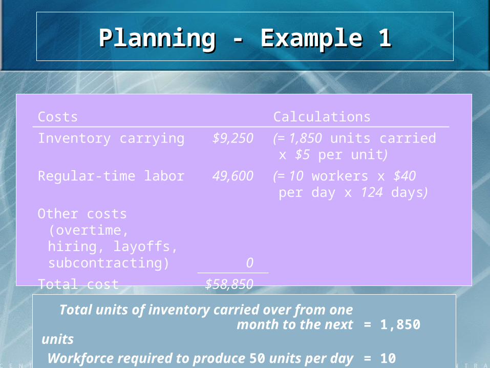
Table 13.3Table 13.3Total units of inventory carried over from onemonth to the next = 1,850 units

Workforce required to produce 50 units per day = 10 workers

Costs Calculations

Inventory carrying $9,250 (= 1,850 units carried x $5 per unit)

Regular-time labor 49,600 (= 10 workers x $40 per day x 124 days)

Other costs (overtime, hiring, layoffs, subcontracting) 0

Total cost $58,850


Cu

mu

lati

ve d

eman

d u

nit

sC

um

ula

tive

dem

and

un

its

7,000 7,000 –

6,000 6,000 –

5,000 5,000 –

4,000 4,000 –

3,000 3,000 –

2,000 –

1,000 –

–JanJan FebFeb MarMar AprApr MayMay JuneJune

Cumulative forecast Cumulative forecast requirementsrequirements

Cumulative level Cumulative level production using production using average monthly average monthly

forecast forecast requirementsrequirements

Reduction Reduction of inventoryof inventory

Excess inventoryExcess inventory





JanJan 900900 2222 4141

FebFeb 700700 1818 3939

MarMar 800800 2121 3838

AprApr 1,2001,200 2121 5757

MayMay 1,5001,500 2222 6868

JuneJune 1,1001,100 2020 5555

6,2006,200 124124

Minimum requirementMinimum requirement = 38 = 38 units per day units per day


70 70 –

60 60 –

50 50 –

40 40 –

30 30 –



Pro

du

ctio

n r

ate

per

wo

rkin

g d

ayP

rod

uct

ion

rat

e p

er w

ork

ing

day

Level production Level production using lowest using lowest

monthly forecast monthly forecast demanddemand

Forecast demandForecast demand


In-house production = 38 units per day x 124 days

= 4,712 units

Subcontract units = 6,200 - 4,712= 1,488 units




Inventory carry costInventory carry cost $ 5$ 5 per unit per month per unit per month










In-house production = 38 units per day x 124 days

= 4,712 units

Subcontract units = 6,200 - 4,712= 1,488 units

Costs Calculations

Regular-time labor $37,696 (= 7.6 workers x $40 per day x 124 days)

Subcontracting 14,880 (= 1,488 units x $10 per unit)

Total cost $52,576





JanJan 900900 2222 4141

FebFeb 700700 1818 3939

MarMar 800800 2121 3838

AprApr 1,2001,200 2121 5757

MayMay 1,5001,500 2222 6868

JuneJune 1,1001,100 2020 5555

6,2006,200 124124

Production = Expected DemandProduction = Expected Demand


70 70 –

60 60 –

50 50 –

40 40 –

30 30 –



Pro

du

ctio

n r

ate

per

wo

rkin

g d

ayP

rod

uct

ion

rat

e p

er w

ork

ing

day Forecast demand and Forecast demand and

monthly productionmonthly production














MonthForecast (units)

Daily Prod Rate

Basic Production

Cost (demand x 1.6 hrs/unit

x $5/hr)

Extra Cost of Increasing Production

(hiring cost)

Extra Cost of Decreasing Production (layoff cost)

Total Cost

Jan 900 41 $ 7,200 — — $ 7,200

Feb 700 39 5,600 —$1,200

(= 2 x $600)6,800

Mar 800 38 6,400 —$600

(= 1 x $600)7,000

Apr 1,200 57 9,600$5,700

(= 19 x $300)— 15,300

May 1,500 68 12,000$3,300

(= 11 x $300)— 15,300

June 1,100 55 8,800 —$7,800

(= 13 x $600)16,600

$49,600 $9,000 $9,600 $68,200


Comparison of Three PlansComparison of Three Plans

CostCost Plan 1Plan 1 Plan 2Plan 2 Plan 3Plan 3

Inventory carryingInventory carrying $ 9,250$ 9,250 $ 0$ 0 $ 0$ 0

Regular laborRegular labor 49,60049,600 37,69637,696 49,60049,600

Overtime laborOvertime labor 00 00 00

HiringHiring 00 00 9,0009,000

LayoffsLayoffs 00 00 9,6009,600

SubcontractingSubcontracting 00 00 00

Total costTotal cost $58,850$58,850 $52,576$52,576 $68,200$68,200

Plan 2 is the lowest cost optionPlan 2 is the lowest cost option

Mathematical ApproachesMathematical Approaches

Useful for generating strategiesUseful for generating strategies Transportation Method of Linear Transportation Method of Linear

ProgrammingProgramming Produces an optimal planProduces an optimal plan

Management Coefficients ModelManagement Coefficients Model Model built around manager’s Model built around manager’s

experience and performanceexperience and performance

Other ModelsOther Models Linear Decision RuleLinear Decision Rule

SimulationSimulation

General Linear Programming (LP) Model

LP gives an optimal solution, but demand and costs must be linear

Let Wt = workforce size for period t Pt =units produced in period t It =units in inventory at the end of

period t Ft =number of workers fired for period t Ht = number of workers hired for period

t

LP MODELMinimize Z = $100 (H1 + H2 + H3 + H4)

+ $500 (F1 + F2 + F3 + F4)

+ $0.50 (I1 + I2 + I3 + I4)

Subject to

P1 - I1 = 80,000 (1)

Demand I1 + P2 - I2 = 50,000 (2)

constraints I2 + P3 - I3 = 120,000 (3)

I3 + P4 - I4 = 150,000 (4)

Production 1000 W1 = P1 (5)

constraints 1000 W2 = P2 (6)

1000 W3 = P3 (7)

1000 W4 = P4 (8)

100 + H1 - F1 = W1 (9)

Work force W1 + H2 - F2 = W2 (10)

constraints W2 + H3 - F3 = W3 (11)

W3 + H4 - F4 = W4 (12)

Transportation Method- Example Transportation Method- Example 11

11 900900 10001000 100100 50050022 15001500 12001200 150150 50050033 16001600 13001300 200200 50050044 30003000 13001300 200200 500500

Regular production cost per unitRegular production cost per unit $20$20Overtime production cost per unitOvertime production cost per unit $25$25Subcontracting cost per unitSubcontracting cost per unit $28$28Inventory holding cost per unit per periodInventory holding cost per unit per period $3$3Beginning inventoryBeginning inventory 300 units300 units

EXPECTEDEXPECTED REGULARREGULAR OVERTIMEOVERTIME SUBCONTRACTSUBCONTRACTQUARTERQUARTER DEMANDDEMAND CAPACITYCAPACITY CAPACITYCAPACITY CAPACITYCAPACITY

Transportation TableauTransportation Tableau

UnusedPERIOD OF PRODUCTION 1 2 3 4 Capacity Capacity

Beginning 0 3 6 9

Inventory 300 — — — 300

Regular 600 300 100 — 1000

Overtime 100 100

Subcontract 500

Regular 1200 — — 1200

Overtime 150 150

Subcontract 250 250 500

Regular 1300 — 1300

Overtime 200 — 200

Subcontract 500 500

Regular 1300 1300

Overtime 200 200

Subcontract 500 500

Demand 900 1500 1600 3000 250

1

2

3

4

PERIOD OF USE

20 23 26 29

25 28 31 34

28 31 34 37

20 23 26

25 28 31

28 31 34

20 23

25 28

28 31

20

25

28

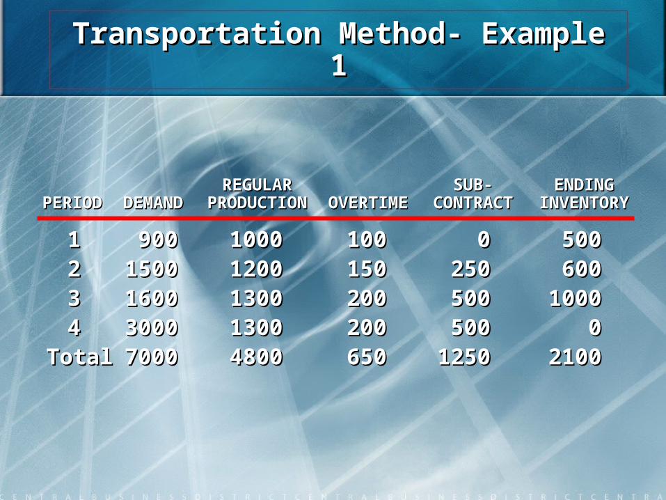
11 900900 10001000 100100 00 50050022 15001500 12001200 150150 250250 60060033 16001600 13001300 200200 500500 1000100044 30003000 13001300 200200 500500 00

TotalTotal 70007000 48004800 650650 12501250 21002100

REGULARREGULAR SUB-SUB- ENDINGENDINGPERIODPERIOD DEMANDDEMAND PRODUCTIONPRODUCTION OVERTIMEOVERTIME CONTRACTCONTRACT INVENTORYINVENTORY


Sales PeriodSales PeriodMarMar AprApr MayMay

DemandDemand 800800 1,0001,000 750750Capacity:Capacity: RegularRegular 700700 700700 700700 OvertimeOvertime 5050 5050 5050 SubcontractingSubcontracting 150150 150150 130130Beginning inventoryBeginning inventory 100100 tires tires

CostsCostsRegular timeRegular time $40$40 per tireper tireOvertimeOvertime $50$50 per tireper tireSubcontractingSubcontracting $70$70 per tireper tireCarryingCarrying $ 2$ 2 per tireper tire


Important pointsImportant points

1.1. Carrying costs are Carrying costs are $2$2/tire/month. If /tire/month. If goods are made in one period and held goods are made in one period and held over to the next, holding costs are over to the next, holding costs are incurredincurred

2.2. Supply must equal demand, so a Supply must equal demand, so a dummy column called “unused dummy column called “unused capacity” is addedcapacity” is added

3.3. Because back ordering is not viable in Because back ordering is not viable in this example, cells that might be used to this example, cells that might be used to satisfy earlier demand are not availablesatisfy earlier demand are not available


Important pointsImportant points

4.4. Quantities in each column designate the Quantities in each column designate the levels of inventory needed to meet levels of inventory needed to meet demand requirementsdemand requirements

5.5. In general, production should be In general, production should be allocated to the lowest cost cell allocated to the lowest cost cell available without exceeding unused available without exceeding unused capacity in the row or demand in the capacity in the row or demand in the columncolumn

Transportation Method- Example 2Transportation Method- Example 2

Management Coefficients Management Coefficients ModelModel

Builds a model based on manager’s Builds a model based on manager’s experience and performanceexperience and performance

A regression model is constructed A regression model is constructed to define the relationships between to define the relationships between decision variablesdecision variables

Objective is to remove Objective is to remove inconsistencies in decision makinginconsistencies in decision making

Other Quantitative Other Quantitative TechniquesTechniques

Linear decision rule (LDR)Linear decision rule (LDR) Search decision rule (SDR)Search decision rule (SDR) Management coefficients modelManagement coefficients model

Hierarchical Nature of Planning

ItemsItems

Product lines Product lines or familiesor families

Individual Individual productsproducts

ComponentsComponents

Manufacturing Manufacturing operationsoperations

Resource Resource LevelLevel

PlantsPlants

Individual Individual machinesmachines

Critical Critical work work

centerscenters

Production Production PlanningPlanning

Capacity Capacity PlanningPlanning

Resource requirements

plan

Rough-cut capacity

plan

Capacity requirements

plan

Input/ output control

Aggregate production

plan

Master production schedule

Material requirements

plan

Shop floor

schedule

All All work work

centerscenters

Available-to-Promise (ATP)

Quantity of items that can be promised to Quantity of items that can be promised to the customerthe customer

Difference between planned production Difference between planned production and customer orders already receivedand customer orders already received

AT in period 1 = (On-hand quantity + MPS in period 1) –

- (CO until the next period of planned production)

ATP in period n = (MPS in period n) –

- (CO until the next period of planned production)

ATP: ExampleATP: Example

ATP: ExampleATP: Example (cont.) (cont.)

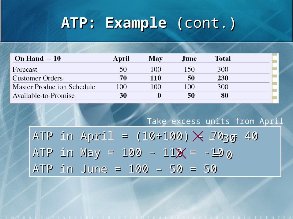
ATP: ExampleATP: Example (cont.) (cont.)

ATP in April = (10+100) – 70 = 40ATP in April = (10+100) – 70 = 40

ATP in May = 100 – 110 = -10ATP in May = 100 – 110 = -10

ATP in June = 100 – 50 = 50ATP in June = 100 – 50 = 50

= 30= 30

= 0= 0

Take excess units from April

Rule Based ATPRule Based ATPProduct Request

Is the product available at

this location?

Is an alternative product available

at an alternate location?

Is an alternative product available at this location?

Is this product available at a

different location?

Available-to-promise

Allocate inventory

Capable-to-promise date

Is the customer willing to wait for

the product?

Available-to-promise

Allocate inventory

Revise master schedule

Trigger production

Lose sale

YesYes

NoNo

YesYes

NoNo

YesYes

NoNo

YesYes

NoNo

YesYes

NoNo

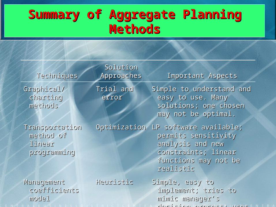
Summary of Aggregate Planning Summary of Aggregate Planning MethodsMethods

TechniquesTechniquesSolution Solution

ApproachesApproaches Important AspectsImportant Aspects

Graphical/charting Graphical/charting methodsmethods

Trial and errorTrial and error Simple to understand and Simple to understand and easy to use. Many easy to use. Many solutions; one chosen may solutions; one chosen may not be optimal.not be optimal.

Transportation Transportation method of linear method of linear programmingprogramming

OptimizationOptimization LP software available; LP software available; permits sensitivity analysis permits sensitivity analysis and new constraints; linear and new constraints; linear functions may not be functions may not be realisticrealistic

Management Management coefficients coefficients modelmodel

HeuristicHeuristic Simple, easy to implement; Simple, easy to implement; tries to mimic manager’s tries to mimic manager’s decision process; uses decision process; uses regressionregression

Aggregate Planning for ServicesAggregate Planning for Services

1.1. Most services can’t be inventoriedMost services can’t be inventoried

2.2. Demand for services is difficult to predictDemand for services is difficult to predict

3.3. Capacity is also difficult to predictCapacity is also difficult to predict

4.4. Service capacity must be provided at the Service capacity must be provided at the appropriate place and timeappropriate place and time

5.5. Labor is usually the most constraining Labor is usually the most constraining resource for servicesresource for services

Controlling the cost of labor is criticalControlling the cost of labor is critical

1.1. Close scheduling of labor-hours to Close scheduling of labor-hours to assure quick response to customer assure quick response to customer demanddemand

2.2. Some form of on-call labor resourceSome form of on-call labor resource

3.3. Flexibility of individual worker skillsFlexibility of individual worker skills

4.4. Individual worker flexibility in rate of Individual worker flexibility in rate of output or hoursoutput or hours

Aggregate Planning for Aggregate Planning for ServicesServices

Law Firm ExampleLaw Firm Example

(3)(3) (4)(4) (5)(5) (6)(6)(1)(1) (2)(2) LikelyLikely WorstWorst MaximumMaximum Number ofNumber of

Category ofCategory of Best CaseBest Case CaseCase CaseCase Demand inDemand in QualifiedQualifiedLegal BusinessLegal Business (hours)(hours) (hours)(hours) (hours)(hours) PeoplePeople PersonnelPersonnel

Trial workTrial work 1,8001,800 1,5001,500 1,2001,200 3.63.6 44Legal researchLegal research 4,5004,500 4,0004,000 3,5003,500 9.09.0 3232Corporate lawCorporate law 8,0008,000 7,0007,000 6,5006,500 16.016.0 1515Real estate lawReal estate law 1,7001,700 1,5001,500 1,3001,300 3.43.4 66Criminal lawCriminal law 3,5003,500 3,0003,000 2,5002,500 7.07.0 1212

Total hoursTotal hours 19,50019,500 17,00017,000 15,00015,000Lawyers neededLawyers needed 3939 3434 3030

Yield ManagementYield Management

Allocating resources to customers at Allocating resources to customers at prices that will maximize yield or prices that will maximize yield or revenuerevenue

1.1. Service or product can be sold in advance of Service or product can be sold in advance of consumptionconsumption

2.2. Demand fluctuatesDemand fluctuates

3.3. Capacity is relatively fixedCapacity is relatively fixed

4.4. Demand can be segmentedDemand can be segmented

5.5. Variable costs are low and fixed costs are highVariable costs are low and fixed costs are high

Yield Management

Yield Management (cont.)

Yield Management:Yield Management: Example-1Example-1

NO-SHOWSNO-SHOWS PROBABILITYPROBABILITY PP((NN < < XX))

00 .15.15 .00.0011 .25.25 .15.1522 .30.30 .40.4033 .30.30 .70.70

Optimal probability of no-showsOptimal probability of no-shows

P(P(nn < < xx) ) = = .517 = = .517CCuu

CCuu + + CCoo

757575 + 7075 + 70

.517.517

Hotel should be overbooked by two rooms

Demand Demand CurveCurve

Yield ManagementYield Management : Example- : Example-22

Passed-up contribution

Money left on the table

Potential customers exist who Potential customers exist who are willing to pay more than the are willing to pay more than the $15$15 variable cost of the room variable cost of the room

Some customers who paid Some customers who paid $150$150 were actually willing were actually willing to pay more for the roomto pay more for the room

$ $ marginmargin ==((PricePrice)) x x (50(50roomsrooms))==($150 - $15)($150 - $15)x x (50)(50)==$6,750$6,750

PricePrice

Room salesRoom sales

100100

5050

$150$150Price charged Price charged

for room for room

$15$15Variable costVariable cost

of roomof room

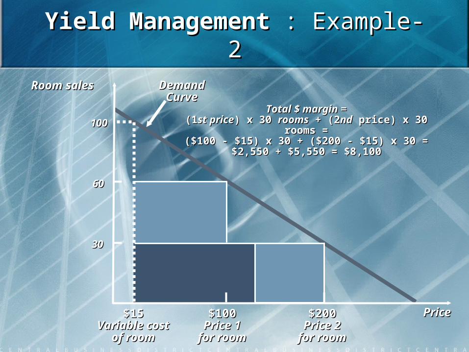
Total $ margin =Total $ margin =(1(1st pricest price) x 30 ) x 30 roomsrooms + (2 + (2ndnd price) x 30 rooms = price) x 30 rooms =

($100 - $15) x 30 + ($200 - $15) x 30 =($100 - $15) x 30 + ($200 - $15) x 30 =$2,550 + $5,550 = $8,100$2,550 + $5,550 = $8,100

Demand Demand CurveCurve

PricePrice

Room salesRoom sales

100100

6060

3030

$100$100Price 1Price 1

for roomfor room

$200$200Price 2Price 2

for roomfor room

$15$15Variable costVariable cost

of roomof room

Yield ManagementYield Management : Example- : Example-22

Yield Management MatrixYield Management Matrix

Du

rati

on

of

use

Un

pre

dic

tab

le

Pre

dic

tab

le

Price

Tend to be fixed Tend to be variable

Quadrant 1: Quadrant 2:

Movies HotelsStadiums/arenas Airlines

Convention centers Rental carsHotel meeting space Cruise lines

Quadrant 3: Quadrant 4:

Restaurants Continuing careGolf courses hospitals

Internet serviceproviders

72

Making Yield Management WorkMaking Yield Management Work

1.1. Multiple pricing structures must be Multiple pricing structures must be feasible and appear logical to the feasible and appear logical to the customercustomer

2.2. Forecasts of the use and duration of Forecasts of the use and duration of useuse

3.3. Changes in demandChanges in demand

TIME - BREAKTIME - BREAK

aggregate planning objective is to minimize cost over the planning period by adjusting production...

Documents

demand slide

demand overtime

aggregate planning slide

capacity slide

high demand

demand research

forecast of demand

low demand periods