Agenda

1. Housekeeping: readings, team name & e-e-mail, etc.

2. News1. Surveillance data mining2. Shopping basket analysis

3. Segmentation marketing1. Basics of segmentation2. Geographics 3. Demographics4. Lifecycle5. Cohorts6. Psychographics & behavior

4. Team discussion questions1. Profile yourself as consumer2. Profile your customers: How does this enable you to

respond to their needs better5. Next week: consumer behavior– why we buy what we buy

Use the various consumer profiling methods to:

1. Profile yourself as a consumer (use VALS-2, Prism, and other demographic, psychographic, and lifestyle descriptors).

2. What are the implications for marketers (e.g., how is this reflected in how they do/can market to you more effectively)?

3. Profile the customers in your business (or department).

4. How does this information about your customers enable you to provide better products/services to them?

5. What more do you need to know? How could you find out?

Group discussion questions for tonight

You might understand the parts, but might miss the whole chicken

What is?

Demographic/Geographic refers to age, sex, income, education, race, martial status, size of household, geographic location, size of city, and profession.

Life stage refers to chronological benchmarking of people's lives at different ages (e.g., pre-teens, teenagers, empty-nesters, etc.).

Lifestyle refers to the collective choice of hobbies, recreational pursuits, entertainment, vacations, and other non-work time pursuits

Psychographics refers to personality and emotionally based behavior linked to purchase choices; for example, whether customers are risk-takers or risk-avoiders, impulsive buyers, etc.

Belief and value systems includes religious, political, nationalistic, and cultural beliefs and values.

Behavior analysis includes what behaviors consumers actually engage in (after all is said and done)

Methods of Seg-men-ta-tion

Requirements for segmentation

Question: What are some criteria that could be used to ensure that a segmentation has utility?

Identifiable: the differentiating attributes of the segments must be measurable so that they can be identified.

Relevant/Accessible: the segments must be reachable through communication and distribution channels.

Substantial: the segments should be sufficiently large to justify the resources required to target them.

Unique needs: to justify separate offerings, the segments must respond differently to the different marketing mixes.

Durable: the segments should be relatively stable to minimize the cost of frequent changes.

Pitfalls of Segmentation

• appeal to segments that are too small

• misread consumer similarities and differences

• become cost inefficient

• spin off too many imitations of their original products or brands

• become short-run rather than long-run oriented

• unable to use certain media (due to small segment size)

• compete in too many markets

• confuse people

• become locked in to a declining market

• too slow to seek innovation possibilities for new products

Demographic Profile

Business segmentation can help companies align their sales territories based on the opportunitieson the ground. The BEFOREmap shows territories determine by geometry—four quadrants dividing the central area—while the AFTERmap shows territories that vary in size based on the number andpotential value of target businesses (the red dots indicating the locations of target businesses). Bymapping its business prospects by size and industry type in Lexington, Kentucky, a company canbetter realign its sales territories based on the concentrations of its high-quality prospects.

In online communities, who are the influencers?

Social Network Analysis

The Hypernetworked World

Profile of Motor Boat Owner Segmentation

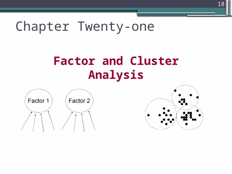
Chapter Twenty-one

18

Factor and Cluster Analysis

Factor Analysis

•Combines questions or variables to create new factors

•Combines objects to create new groups

Uses in Data Analysis

▫ To identify underlying constructs in the data from the groupings of variables that emerge

▫ To reduce the number of variables to a more manageable set

19

Factor Analysis (Contd.)

Methodology

•Principal Component Analysis

▫Summarizes information in a larger set of variables to a smaller set of factors

•Common Factor Analysis

▫Uncovers underlying dimensions surrounding the original variables

20

Factor Analysis - Example

21

Export Data Set - Illustration

22

Respid Will(y1) Govt(y2) Train(x5) Size(x1) Exp(x6) Rev(x2) Years(x3)

Prod(x4)

1 4 5 1 49 1 1000 5.5 6

2 3 4 1 46 1 1000 6.5 4

3 5 4 1 54 1 1000 6.0 7

4 2 3 1 31 0 3000 6.0 5

5 4 3 1 50 1 2000 6.5 7

6 5 4 1 69 1 1000 5.5 9

. . . . . . . . .

. . . . . . . . .

. . . . . . . . .

115 4 3 1 45 1 2000 6.0 6

116 5 4 1 44 1 2000 5.8 11

117 3 4 1 46 0 1000 7.0 3

118 3 4 1 54 1 1000 7.0 4

119 4 3 1 49 1 1000 6.5 7

120 4 5 1 54 1 4000 6.5 7

Description of Variables

23

Variable Description Corresponding Name in Output

Scale Values

Willingness to Export (Y1) Will 1(definitely not interested) to 5 (definitely interested)

Level of Interest in Seeking Govt Assistance (Y2)

Govt 1(definitely not interested) to 5 (definitely interested)

Employee Size (X1) Size Greater than Zero

Firm Revenue (X2) Rev In millions of dollars

Years of Operation in the Domestic Market (X3)

Years Actual number of years

Number of Products Currently Produced by the Firm (X4)

Prod Actual number

Training of Employees (X5) Train 0 (no formal program) or 1 (existence of a formal program)

Management Experience in International Operation (X6)

Exp 0 (no experience) or 1 (presence of experience)

Factors

Factor

▫ A variable or construct that is not directly observable but needs to be inferred from the input variables

▫ All included factors (prior to rotation) must explain at least as much variance as an “average variable”

Eigenvalue Criteria

▫ Represents the amount of variance in the original variables that is associated with a factor

▫ Sum of the square of the factor loadings of each variable on a factor represents the eigenvalue

▫ Only factors with eigenvalues greater than 1.0 are retained

24

How Many Factors - Criteria

Scree Plot Criteria

▫A plot of the eigenvalues against the number of factors, in order of extraction.

▫ The shape of the plot determines the number of factors

25

How Many Factors: Criteria (Contd.)

Percentage of Variance Criteria

▫The number of factors extracted is determined so

that the cumulative percentage of variance

extracted by the factors reaches a satisfactory

level

Significance Test Criteria

▫Statistical significance of the separate

eigenvalues is determined, and only those factors

that are statistically significant are retained

26

Extraction using Principal Component Method - Unrotated

Component Matrix(a)

Component

1 2 x5 .566 .724 x1 .880 .022 x6 .695 -.344 x2 -.100 .503 x3 -.297 .809 x4 .806 .124

Extraction Method: Principal Component Analysis. a 2 components extracted.

Total Variance Explained

Initial Eigenvalues Extraction Sums of Squared Loadings

Component Total % of Variance Cumulative % Total % of Variance Cumulative % 1 2.326 38.761 38.761 2.326 38.761 38.761 2 1.567 26.109 64.870 1.567 26.109 64.870 3 .918 15.306 80.175 4 .594 9.894 90.069 5 .362 6.035 96.104 6 .234 3.896 100.000

Extraction Method: Principal Component Analysis.

Component Score Coefficient Matrix

Component 1 2 x5 .244 .462 x1 .378 .014 x6 .299 -.220 x2 -.043 .321 x3 -.128 .517 x4 .347 .079

Extraction Method: Principal Component Analysis. Component Scores.

27

Factor Loadings Factor Score Coefficient

Extraction using Principal Component Method - Factor Rotation

28

Total Variance Explained

Initial Eigenvalues Extraction Sums of Squared Loadings Rotation Sums of Squared Loadings

Component Total % of Variance Cumulative % Total % of Variance Cumulative % Total % of Variance Cumulative % 1 2.326 38.761 38.761 2.326 38.761 38.761 2.309 38.479 38.479 2 1.567 26.109 64.870 1.567 26.109 64.870 1.583 26.391 64.870 3 .918 15.306 80.175 4 .594 9.894 90.069 5 .362 6.035 96.104 6 .234 3.896 100.000

Extraction Method: Principal Component Analysis.

Component Score Coefficient Matrix

Component

1 2 x5 .310 .421 x1 .376 -.043 x6 .263 -.262 x2 .006 .324 x3 -.049 .530 x4 .355 .027

Extraction Method: Principal Component Analysis. Rotation Method: Varimax with Kaiser Normalization. Component Scores.

Rotated Component Matrix(a)

Component

1 2 x5 .668 .632 x1 .873 -.110 x6 .636 -.444 x2 -.023 .512 x3 -.173 .844 x4 .816 .002

Extraction Method: Principal Component Analysis. Rotation Method: Varimax with Kaiser Normalization. a Rotation converged in 3 iterations.

Not significantly different from unrotated values

Common Factor Analysis

▫ The factor extraction procedure is similar to that of principal component analysis except for the input correlation matrix

▫ Communalities or shared variance is inserted in the diagonal instead of unities in the original variable correlation matrix

▫ The total amount of variance that can be explained by all the factors in common factor analysis is the sum of the diagonal elements in the correlation matrix

▫ The output of common factor analysis depends on the amount of shared variance

29

Common Factor Analysis – Results (Contd.)

30

Common Factor Analysis - Results

31

Common Factor Analysis – Results (Contd.)

32

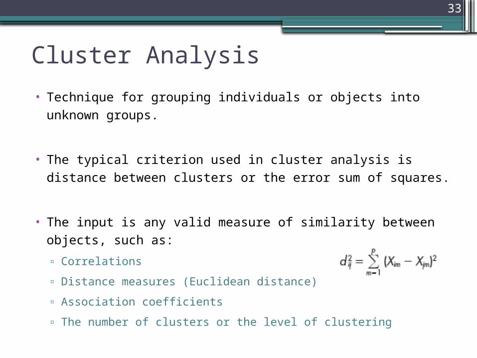
Cluster Analysis

• Technique for grouping individuals or objects into unknown groups.

• The typical criterion used in cluster analysis is distance between clusters or the error sum of squares.

• The input is any valid measure of similarity between objects, such as:

▫ Correlations

▫ Distance measures (Euclidean distance)

▫ Association coefficients

▫ The number of clusters or the level of clustering

33

Steps in Cluster Analysis

Define the problem

Decide on the

appropriate similarity measure

Decide on how to

group the objects

Decide the number of clusters

Interpret, describe,

and validate the clusters

34

Cluster Analysis (Contd.)

Hierarchical Clustering

▫ Can start with all objects in one cluster and divide and subdivide them

until all objects are in their own single-object cluster ( ‘top-down’ or

decision approach)

▫ Can start with each object in its own single-object cluster and

systematically combine clusters until all objects are in one cluster

(‘bottom-up’ or agglomerative approach)

Non-hierarchical Clustering

▫ Permits objects to leave one cluster and join another as clusters are being formed

▫ A cluster center is initially selected and all the objects within a pre-specified threshold distance are included in that cluster

35

Hierarchical Clustering

• Single Linkage▫ Clustering criterion

based on the shortest distance

• Complete Linkage▫ Clustering criterion

based on the longest distance

36

Hierarchical Clustering (Contd.)

• Average Linkage▫ Clustering criterion

based on the average distance

• Ward's Method

▫ Based on the loss of information resulting from grouping of the objects into clusters (minimize within cluster variation)

37

Hierarchical Clustering (Contd.)

• Centroid Method

▫Based on the distance between the group centroids (the point whose coordinates are the means of all the observations in the cluster)

38

Hierarchical Cluster Analysis - Example

39

Hierarchical Cluster Analysis (Contd.)

40

A dendrogram for hierarchical clustering of bank data

Hierarchical Cluster Analysis (Contd.)

41

▫ Number of clusters is specified by the analyst for theoretical or practical reasons.

▫ Level of clustering with respect to clustering criterion is specified.

▫ Determine the number of clusters from the pattern of clusters generated. The distances between clusters or error variability measure at successive steps can be used to decide the number of clusters (from the plot of error sum of squares with the number of clusters).

▫ The ratio of total within-group variance to between group variance is plotted against the number of clusters and the point at which an elbow occurs indicates the number of clusters.

42

Criteria for Determining the Number of Clusters

Assumptions◦ The basic measure of similarity on which the clustering is

based is a valid measure of the similarity between the objects.

◦ There is theoretical justification for structuring the objects into clusters

Limitations◦ It is difficult to evaluate the quality of the clustering◦ It is difficult to know exactly which clusters are very similar

and which objects are difficult to assign.◦ It is difficult to select a clustering criterion and program on

any basis other than availability.43

Assumptions and Limitations of Cluster Analysis