aerosol effects on cloud-precipitation and land … · aerosol effects on cloud-precipitation and...

Toshihisa MatsuiDepartment of Atmospheric Science

Colorado State UniversityFt. Collins, CO 80523-1371, USA

Aerosol Effects on Cloud-Precipitation and Land-Surface Processes

Big Acknowledgements

This entire Ph.D. work is funded by NASA-CSU CEAS fellowship (NAG512105), NASA Radiation (NNG04GB87G), and NASA Interdisciplinary Sciences (NNG04GL61G). Myspecial thanks go to my family, Miwa and Schunta Matsui, for their unconditional love and enduring support; my advisors, Roger A. Pielke and Wei-Kuo Tao, for their great mentorship and funding support; my Ph.D. committees and collaborators, Sonia Kreidenweis, Dev Niyogi, Michael Coughenour, and A. Scott Denning, for their excellent academic and research guidance; Pielke’s research groups, Adriana Beltrán-Przekurat, Chris Castro, Glen Liston, John Lin, Chris Hiemistra, Giovanni Leoncini, Ji-Wang Wang, John Strack, Cartis Martial, David Stokowski, and Dallas Staley, for spending wonderful research time; department stuffs including Melissa Tucker, Jen Weingardt, and Marilyn Hanson, for their assist of my administration processes; department colleagues, Tak Yamaguchi, K.D. Corbin, Derek Posselt, Ian Baker, Lixing Lu, Gustavo Cario, Sue Van Den Heever, Hong-Li Jiang, Kevin Schaefer, for useful discussion in diverse research topics; department professors, Bill Cotton, Chris Kummerow, Wayne Schubert and Graeme Stephens for their academic classes and useful discussions; NASA GSFC’s colleagues, Mian Chin, Lorein Remer, Allen Chu, Steve Lang, Hongbin Yu, Eric Moody, Brian Cosgrove, Kristi Arsenault, Jim Geyger and Sujay Kumar, for their cutting-edge research skill and collaborations; computer system administrators: Tony Arcieri, Sloan Johnson and Michael Aumock for their patience of teaching computer skill to me. In addition, the first half of this dissertation (aerosol-cloud interactions) was strongly inspired by Yoram Kaufman at NASA GSFC, who was accidentally passed away in spring 2006, and Hirohiko Masunaga, a former CSU scientist and a new professor in Nagoya University.

Introduction of Aerosol Effects

• Atmospheric aerosols, suspended atmospheric particles, derive from natural sources and from anthropogenic sources, and are characterized by different compositions, sizes, and shapes.

• In the last century, increases in world population have drastically increased the amount of aerosol emissions from anthropogenic sources [IPCC 2001].

• Aerosols and their effects on climate have increased attention from the science community, because of their proposed counter impact against the warming effect of anthropogenic greenhouse gases (GHGs) [Anderson et al. 2003].

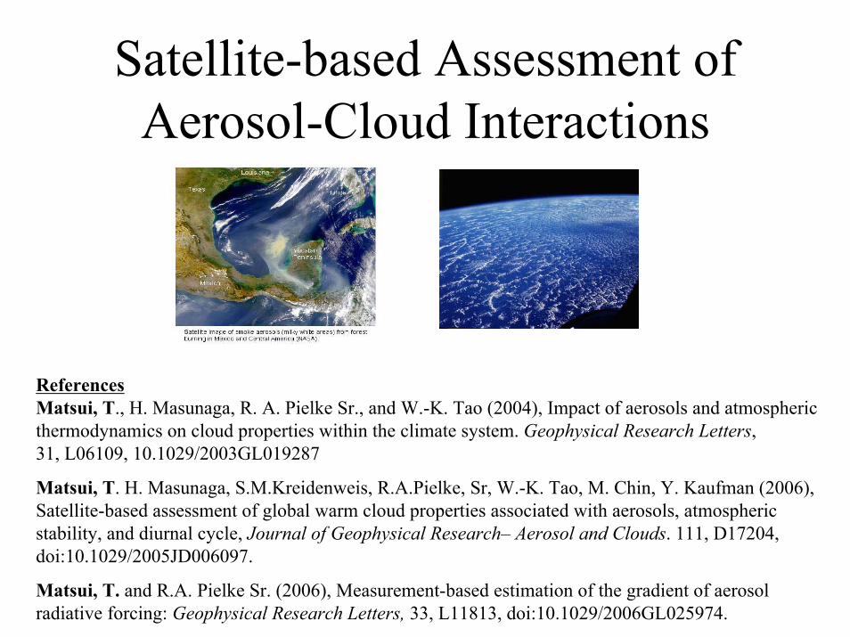
Satellite-based Assessment of Aerosol-Cloud Interactions

ReferencesMatsui, T., H. Masunaga, R. A. Pielke Sr., and W.-K. Tao (2004), Impact of aerosols and atmospheric thermodynamics on cloud properties within the climate system. Geophysical Research Letters, 31, L06109, 10.1029/2003GL019287

Matsui, T. H. Masunaga, S.M.Kreidenweis, R.A.Pielke, Sr, W.-K. Tao, M. Chin, Y. Kaufman (2006), Satellite-based assessment of global warm cloud properties associated with aerosols, atmospheric stability, and diurnal cycle, Journal of Geophysical Research– Aerosol and Clouds. 111, D17204, doi:10.1029/2005JD006097.

Matsui, T. and R.A. Pielke Sr. (2006), Measurement-based estimation of the gradient of aerosol radiative forcing: Geophysical Research Letters, 33, L11813, doi:10.1029/2006GL025974.

Atmospheric Aerosols

Cloud formation

Water Cycle Energy CycleAerosol Dynamic Effect

PrecipitationProcess

Aerosol Indirect Effect

Direct Absorption &Scattering of SW

Atmospheric Radiation Budget

Aerosol Direct Effect

Aerosols and Warm Rain Process• Amount of marine low clouds is strongly controlled by the thermodynamics, which

is represented by lower-tropospheric stability (LTS) [Klein 1996].

• Aerosols also control marine low clouds properties by acting as cloud condensation nuclei (CCN) to form cloud droplets. A high conenctrations of aerosols tends to reduce mean size of cloud droplet size [Kaufman and Fraser 1997; Nakajima et al.2001; Bréon et al. 2002 ] and warm rain process [Rosenfeld 1999].

Question• How are mean size of cloud droplet and warm-rain process distributed and related to

aerosol concentrations as well as thermodynamics on the large scale?

ReferencesMatsui, T., H. Masunaga, R. A. Pielke Sr., and W.-K. Tao (2004), Impact of aerosols

and atmospheric thermodynamics on cloud properties within the climate system. Geophysical Research Letters, 31, L06109, 10.1029/2003GL019287

Marine Low Cloud Properties (Ttop > 273K)

MW

CLWP

VIS

tau

liquid Cloud

NIR

Re(top)

IR

Tc

Re(column)

Ocean

Warm Rain Process• Comparison between

Re(top) and Re(column) at each rid box can be used to diagnose the low cloud mode: non-precipitating, transitional, and precipitating.

• Near-global map of marine liquid cloud mode (Mar-May 2000 statistics).

Precipitating

TransitionalNon-precipitating

Uncertain

Global distribution of non-precipitating, transitional, and precipitating low cloudaveraged through March-May in 2000.

AI and LTS• Aerosol Concentrations Aerosol Index: AI=AOD*ANG [Nakajima et al.

2001] derived from MODIS products in order to account for both aerosol optical depth and size distribution.

• Thermodynamics Lower tropospheric stability (LTS): θ700mb - θsurface[Klein and Hartmann, 1993] derived from NCEP/NCAR reanalysis

Global distribution of aerosol index (dark shaded) and low-troposphere static stability LTS (K) (colored contour) averaged through March-May in 2000.

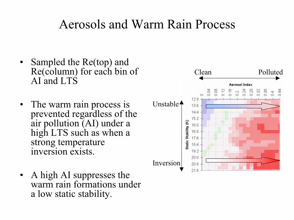
Aerosols and Warm Rain Process

• Sampled the Re(top) and Re(column) for each bin of AI and LTS

• The warm rain process is prevented regardless of the air pollution (AI) under a high LTS such as when a strong temperature inversion exists.

• A high AI suppresses the warm rain formations under a low static stability.

Clean Polluted

Unstable

Inversion

Aerosols and Marine Low Cloud Process

• A high concentration of the aerosols is expected to reduce mean size of cloud droplet, which is expected to increase cloud albedo for a constant liquid water path [Twomey et al. 1984].

• Cloud liquid water is expected to be increased for higher aerosol concentrations due to suppressed drizzle process [Albrecht 1998].

Questions• How is the cloud liquid water path (CLWP) related with variability of aerosol

concentrations?

• Which factor (either aerosols or thermodynamics) is more important to describe variability of marine low cloud properties (Re, CLWP, and cloud fraction)?

Reference

Matsui, T. H. Masunaga, S.M.Kreidenweis, R.A.Pielke, Sr, W.-K. Tao, M. Chin, Y. Kaufman (2006), Satellite-based assessment of global warm cloud properties associated with aerosols, atmospheric stability, and diurnal cycle, Journal of Geophysical Research– Aerosol and Clouds. 111, D17204, doi:10.1029/2005JD006097.

Sampling• Sampling period is from March 2000 to February

2001.

• Sampling number is highly concentrated in subtropics due to TRMM’s unique overpass and natural variability of warm cloud distribution.

• Histograms of MODIS/GOCART AI and NCEP LTS were made. 95 % of the most frequent values of AI and LTS were considered in the statistics.

• The sampling ranges (max and minimum bin) between AI and LTS are the same frequencies in this sampling. This allows us to compare the aerosols and thermodynamics forcing.

• Total sampling number is about 0.7 million.

Case 1: TRMM cloud vs. MODIS AI – NCEP LTS

Case 2: TRMM cloud vs. GOCART AI – NCEP LTS

0

0.02

0.04

0.06

0.08

0.1

0.12

0.14

0 0.1 0.2 0.3 0.4AI

PD

F

MODIS: 95% of range(0.0075 - 0.3825)

GOCART: 95% of range(0.0075 - 0.2525)

95% of range (9.95 - 20.75)

00.0020.0040.0060.0080.01

0.0120.0140.0160.0180.02

5 15 25

LTS (K)

PDF

Sampled 95% of PDF

Global Statitics

10.512.5

14.516.5

18.50.03

0.100.18

0.250.33

810.51315.518

20.5

23

25.5

28

30.5

Re(colum

n) (micron)

NCEP LTS (stability)

MODIS AI

28-30.525.5-2823-25.520.5-2318-20.515.5-1813-15.510.5-138-10.5

10.512.5

14.516.5

18.50.02

0.070.12

0.170.22

810.51315.518

20.5

23

25.5

28

30.5

Re(colum

n) (micron)


GOCART AI

28-30.525.5-2823-25.520.5-2318-20.515.5-1813-15.510.5-138-10.5

• Cloud droplet sizes tend to be smallest in polluted and strong-inversion environment. Variability of AI explains the variability of Re (e.g., warm rain process) about twice as LTS does.

• The cloud liquid water path (CLWP) tends to be smaller for higher AI. These results do not support the hypotheses or assumption of constant or increased CLWP associated with high aerosol concentrations [Twomey 1984, Albrecht1993].

• Corrected cloud albedo (CCA: product of cloud albedo and cloud fraction) appear to be larger for higher LTS. CCA-LTS correlations appear to be stronger than CCA-AI correlation.

10.512.5

14.516.5

18.5 0.030.10

0.180.25

0.33

20

30

40

50

60

70

80

Cloud LW

P (g/m2)


MODIS AI

70-8060-7050-6040-5030-4020-30

10.512.5

14.516.5

18.5 0.020.07

0.120.17

0.22

20

30

40

50

60

70

80

Cloud LW

P (kg/m2)


GOCART AI

70-8060-7050-6040-5030-4020-30

10.5

12.5

14.516.5

18.5

0.030.10

0.180.25

0.330

0.05

0.1

0.15

0.2

albedo


MODIS AI

0.15-0.20.1-0.150.05-0.10-0.05

10.5

12.5

14.516.5

18.5

0.020.07

0.120.17

0.220.1

0.15

0.2

0.25

0.3

0.35

0.4

1-deg Cloud Fraction


GOCART AI

0.35-0.40.3-0.350.25-0.30.2-0.250.15-0.20.1-0.15

Linear correlation coefficient in each 4-degree box on a global grid for the same annual sampling period.Non-sampled grids (over land) and statistically insignificant correlations (approximately, |r| < 0.05) with the

t-distribution critical level set to 0.05 are shown in white.

Diurnal Cycles of Marine Low Cloud Properties

1.92

2.12.22.32.42.52.62.7

7 9 11 13 15 17local time (hour)

clou

d-to

p he

ight

(km

)

101214161820222426


Re(

colu

mn)

(mic

ron)

20

30

40

50

60

70

80


CLW

P (g

/m2)

LTS

0

0.02

0.04

0.06

0.08

0.1

0.12


Cor

rect

ed C

loud

Alb

edo 19.6

17.5

15.4

13.3

11.2

a. Diurnal cycle of cloud properties in different LTS regions

1.92

2.12.22.32.42.52.62.7


clou

d-to

p he

ight

(km

)

101214161820222426


Re(

colu

mn)

(mic

ron)

20

30

40

50

60

70

80


CLW

P (g

/m2)

MODIS AI

0

0.02

0.04

0.06

0.08

0.1

0.12


Cor

rect

ed C

loud

Alb

edo 0.38

0.29

0.21

0.13

0.05

b. Diurnal cycle cloud properties in different AI regions

Spatial Gradient of Aerosol Radiative Forcing

• A science community tends to quantify the aerosol radiative forcing as the global averaged top-of-atmosphere (TOA) value to compare with that of GHGs [Anderson et al. 2003].

Questions• How can a heterogeneous radiative forcing be effectively quantified as

linked to atmospheric circulation and regional climate?

ReferenceMatsui, T. and R.A. Pielke Sr. (2006), Measurement-based estimation of the

gradient of aerosol radiative forcing: Geophysical Research Letters, 33, L11813, doi:10.1029/2006GL025974.

Aerosol Direct Radiative Forcing (ADRF)RADRF = R(currnet AOD) - R(potential

AOD)

• RADRF is estimated in clear-sky conditions.

• The current AOD: the MODIS instantaneous AOD at 0.55 µm and 0.865µm. Total column AOD is subdivided into dust, sea salt, organic carbon, black carbon and sulfate components based on the co-located daily product of GOCART [Chin et al. 2004].

• Potential AOD: the sum of estimated sea salt and dust AOD.

• Aerosol optical properties: Optical Properties of Aerosol and Cloud (OPAC) values [Hess et al. 1998].

Aerosol Indirect Radiative Forcing (AIRF)

RAIRF=R(current cloud properties) -R(potential cloud properties)

• RAIRF is derived without aerosol direct effect. Potential cloud properties (Re, CLWP, and fraction) are estimated as a function of ambient AI for a given LTS, by using the correlation in Matsui et al. [2005].

• The estimation of AIRF accounts for low liquid clouds with cloud top temperatures greater than 273 K.

Spatial Mean Radiative Forcing

• Anthropogenic radiative forcing is currently expressed as the spatial (often on global scale) mean TOA radiative forcing in climate assessment reports.

• This metric is useful for the energy budget of the entire Earth as a closed system.

• Note that GHG radiative forcing (GRF) was estimated from the difference in infrared radiative cooling between pre-industrial and current levels of CO2, N2O , CH4, CFC-11, CFC-12, and CFC-113, respectively.

mean TOA radiative forcing

-1.38-1.591.7

-2

-1

0

1

2

GRF ADRF AIRF

radi

tive

forc

ing

(W/m

2)

Spatial Gradient of Radiative Forcing

• Normalized Gradient of Radiative Forcing (NGoRF) essentially represents the fraction of the present Earth’s heterogeneous insolation attributed to human activity on different horizontal scales.

• E.g., For ADRF, NGoRF is

atmosphere

00.050.1

0.150.2

0 5 10 15 20

NG

oRF

ADRF(zone) AIRF(zone) GRF(zone)ADRF(meri) AIRF(meri) GRF(meri)

total

ADRF

GoRFGoRFNGoRF = surface

00.050.1

0.150.2

0 5 10 15 20distance (degree)

NG

oRF

λ∂∂

= totaltotal

RGoRF

λ∂∂

= ADRFADRF

RGoRF

ReferenceKim, M., and W. Lee (2006), Dynamic feedbacks of troposphere aerosols on marine low cloud during boreal spring, Geophys. Res. Lett., 33, L16704, doi:10.1029/2006GL026351.

•Sensitivity experiments using GEOS fv-GCM with and without ADRF .

•Distribution of (a) aerosol optical thickness (contour) and lower-troposphere static stability (shaded) of NA experiment,

•(b) aerosol induced net radiative forcing (AIRF) at the surface, and

• (c) low-cloud amount anomaly (dCL) during boreal spring.

•Contour intervals in (a), (b), and (c) are 0.05, 10 Wm-2 and 3%, respectively. AIRF and dCL are calculated by the difference between all aerosols experiment (AA) and no aerosol experiment (NA). In (c) contour line of 0% is omitted for simplicity and significance levels are shaded in different colors.

ReferenceTakemura, T., Y. J. Kaufman, L. A. Remer, T. Nakajima (2006), Two competing pathways of aerosols effect on cloud and precipitation formation, Geophysical Research Letter, (submitted).

• 50-year integration of coupled aerosol-atmosphere-ocean model

• A nudged experiment (b) shows the small changes in CLWP and precipitation.

• A free-running experiments (c) shows the large changes in the spatial distributinof CLWP and precipitation.

Summary of Aerosol-Cloud Interactions

• Satellite-based statistical studies indicate that high aerosol concentrations tends to reduce the means size of clouds and precipitation process but simultaneously decrease the cloud liquid water path.

• Stronger correlation between Re and AI (than Re-LTS correlation) indicates the importance of aerosols on warm rain process.

• Stronger correlation between CCA and LTS (than CCA-AI correlation) indicates that the importance of teleconnection on the cloud radiative forcing due to heterogeneous aerosols radiative forcing.

Aerosol Forcing on Land-Surface Process over Eastern U.S.

ReferencesMatsui, T., S. M. Kreidenweis, R.A. Pielke Sr., B. Schichtel, H. Yu, M. Chin, D.A. Chu, and D. Niyogi (2004b), Regional comparison and assimilation of GOCART and MODIS aerosol optical depth across the eastern U.S. Geophysical Research Letters., 31, L21101, doi:10.1029/2004GL021017.

Matsui, T., A. Beltrán-Przekurat, R. A. Pielke Sr., D. Niyogi, and M. B. Coughenour (2006), Continental-scale multi-observation calibration and assessment of Colorado State University Unified Land Mode: Part I. Surface albedo, Journal of Geophysical Research - Biogeoscience. (Accepted)

Matsui, T., A. Beltrán-Przekurat, R. A. Pielke Sr., D. Niyogi, S. A. Denning, M. Coughenour, and Z. Wan (2006d), Mechanistic Response of Plant Productivity and Surface Energy Budget to the Aerosol Direct Effect over Eastern U.S., Using A Well-Calibrated Sun-Shade Canopy Model, Journal of Geophysical Research - Biogeoscience. (in preparation)


Cloud formation




Diffuse Radiation

Water Cycle Energy Cycle Carbon Cycle

Plant Productivity& Carbon sink

Aerosol Diffuse-Radiation Effect

Aerosol Indirect EffectAerosol Direct Effect

Aerosol Dynamic Effect

Aerosol Forcing on Land-Surface Process over Eastern U.S.

Aerosol diffuse-radiation effect• Diffuse solar radiation is absorbed on the

plant canopy more homogeneously than direct radiation is, and is efficiently utilized in the photosynthesis process without exceeding the plant photosynthesis capacity. On the other hand, direct solar radiation is absorbed by the sunlit canopy and usually exceeds the plant photosynthesis capacity around noon [Goudriaan 1977; Gu et al.2002].

• Ground-based observational studies have shown that aerosol loading tends to enhance diffuse radiation and terrestrial CO2 sink over the eastern U.S. [Niyogi et al. 2004; Chang 2004].

Question:• How are the spatio-temporal variations of

aerosol diffuse-diffuse radiation effect on the regional scale, particularly over the eastern United States?

Shad

ed ca

nopy

Sunlit canopy

Light-limited P-capacity-limited

NASA Land Information System

1km MODIS UMD LULC

1km MODIS LAI

FAO sand/clay fractionFluxnet location

CSU ULM has been developed within the NASA GSFC’s Land Information System (LIS) that contains several different LSMs and a wide variety of surface boundary conditions and meteorological forcings. Thus, off-line simulations of LSM can be tested anywhere on globe down to the urban-resolving scale (Peters-Lidard et al. 2004).

• Subgrid #: 1~13 (+1) based on the MODIS LULC class. (+1) indicates the patch allocated for Fluxnet sites if available. Mhe minimum tile fraction is 0.0013 that fully utilize 1km MODIS information.

• LAI: The 1km LAI data are aggregated for each UMD LULC classes on the 0.25°grid map. Fluxnet patch uses the nearest 1km MODIS LAI.

• Initial Soil Moisture: 1-year spun up of control simulation

ReferencePeters-Lidard, C. D., S. Kumar, Y. Tian, J. L. Eastman, and P. Houser, 2004. Global Urban-

Scale Land-Atmosphere Modeling with the Land Information System, Symposium on Planning, Nowcasting, and Forecasting in the Urban Zone, 84th AMS Annual Meeting 11-15 January 2004 Seattle, WA, U.S.A.

NASA GSFC Land Information System

Model Grid

Subgrid 1~13 (+1)LULC-based tunable

parameters

Off-line (uncoupled) simulation

• CSU LSM is run in off-line (uncoupled mode), and is driven by the North American Land Data Assimilation System (NLDAS) and/or ground-truth meteorological field on a one-hour time step.

• NLDAS meteorological forcing consists of following data [Cosgrove et al. 2002]:

Rader-gauge assimilated precipitation: Hourly National Weather Service Doppler radar-based (WSR-88D0) precipitation analyses were used to disaggregate the daily NCEP CPC gauge-based precipitation to produce an hourly observation-based precipitation data set.

GOES-based surface radiation: Surface downwelling solar and thermal radiation is derived from GOES radiation data.

ETA field: Surface air temperatures, water vapor mixing ratios, horizontal winds, and surface pressures are derived from NCEP EDAS output fields.

Merged precipitation

GOES-derived radiationAll above figures from Cogrove et al. (2003)

Separation of SW radiation• A sun-shade canopy scheme

requires the proper separation of solar radiation into diffuse and direct components [Gu et al. 2002].

• Current products provide the broad-band (direct and diffuse) downwelling solar radiation.

• Diffuse radiation fraction, DRF (Rd/Rg, where Rd is diffuse solar irradiance and Rg is total global irradiance at the surface), was estimated from the transmittance (Rg/Rext, where Rext is extra-terrestrial global irradiance) observed at ISIS network [Hicks et al. 1996] .

0.05

0.3

0.55

0.8 0.05

0.25

0.45

0.65

0.85

0

0.2

0.4

0.6

0.8

1

Rd/Rg

Rg/Rext

u

A sun-shade canopy model in ULM

A sun-shade model was developed in the Unified Land Model (ULM). Leaf-level sunlit fraction, photosynthesis capacity, and wind are exponentially profiled from canopy top to bottom (cumulative LAI (x)). These profiles are integrated for sunlit and shaded canopy, which is developed within the CSU Unified Land Model (ULM).

Top (x=0)

Bottom (x=L)

x

Light penetration

xksun

bexf −=)( ∫ −=L xk

sun dxeLAI b

0

xktopcanleaf

neVxV −=)(

xktopcan

ueuxu −=)(

∫ −−=L xkxktop

cansun

can dxeeVV bn

0

∫ −=L xksun

can dxexuu u

0)(

Leaf Sunlit Canopy

∫ −−=L xk

sha dxeLAI b

0)1(

∫ −− −=L xkxktop

cansha

can dxeeVV bn

0)1(

Shaded Canopy

∫ −− −=L xkxktop

canshacan dxeeuu bu

0)1(

A sun-shade canopy model

• A sun-shade canopy model separately prognoses canopy temperature, latent/sensible/CO2flux for sunlit and shaded canopy.

0=−−−= sunsunsunsunsun EHLWSWR

0=−−−= shashashashasha EHLWSWR

Separate Energy Budget Equations

How can we improve the model?Tuning-Oriented Satellite-Hydrology-Integrated (TOSHI) Cycles

Parameter Estimation Model

Update tunable parameters by

Gauss-Marquardt-Levenberg iterations

Errors

Spectral albedo, land surface temperature

CO2, LHF, SHF

If (Ψ (sum of squared deviationbetween model and observation)has no more improvement)

FinishInitial set of tunable

parametersLand Information System

Met

eoro

logi

cal

Forc

ing

point

FLUXNETNLDAS

area

Off

-line

si

mul

atio

n

Xserve G5

Observations

MODIS spectral albedo, land surface temperature

FLUXNET CO2, LHF,

SHF

New set of tunable

parameters

∂∂

∂∂

∂∂

∂∂

=

n

mm

n

pc

pc

pc

pc

J

L

M

MO

M

M

L

1

1

1

1

Maximum performance ~300GFlops

Application of MODIS Surface AlbedoCanopy Energy Budget Equation

• Although the ULM initialization uses a consistent set of the MODIS LAI and LULC data, the ULM does not produce surface spectral albedo that are consistent with the MODIS radiances due to differences in the sophistication and assumptions of the canopy radiative transfer algorithms and soil albedo configurations



MODIS radiance

MODIS albedo

MODIS LULC

2/3-D RTM+ empirical

MODIS LAI

2-stream RTMin LSM

LSMalbedoConsistent?

Tunable Parameters• Tunable coefficients in two-

stream canopy radiative transfer model:

leaf albedo:Stem/dead leaf albedo: Leaf angle projection:

• These parameters determine the upscattering fraction of diffuse and direct radiation in TCRT

• New tunable soil albedo map as a function of the log-normalized difference of maximum leaf area index (Lmax)

• Tunable coefficients:

• Actual albedo interpolates between

NIRleaf

VISleaf ρρ

NIRstem

VISstem ρρ

lχ

)()( lχβτρωβ +=

),()( loo χµβτρωβ +=

ρτρρ

ρ ⋅=+

⋅+⋅= 865.0,

SAILAISAILAI stemleaf

)2.0ln()7ln()2.0ln()ln( max

−−

=LLND

LNDba VISVISVISdry +

=01.0α

NIRNIRVISVIS baba ,,, VISsat

VISdry and αα

Initial Experiment uses initial set of tunable parameters, which is commonly used in the community. This experiment also uses the global soil albedo map from Reynolds et al. (1999)

Tunable parameters of each LULC class before the calibration. Pre-calibration soil albedo uses the global soil albedo map (Reynolds et al. 1999).

Scatter plots and statistics (m: mean, s: standard deviation, and rmse: root mean square error) of the pre-calibration difference (MODIS–ULM) in spectral surface black- and white-sky albedo (×100). X-axis represents the fraction (0.8~1.0) of each land-cover class. VIS and NIR albedo use different scales in y-axis.

Spatial map of pre-calibration differences (MODIS – ULM) in spectral surface black- and white-sky albedos (×100). Note VIS and NIR albedo use different scales.

Post Calibrationwas

implemented from the lessons learned from the first calibration:i) fixed the functional error in diffuse-radiation upscattering fraction, ii) manually fixed the surface albedo for the urban class (0.06 (VIS) and 0.20 (NIR) based on the mean albedo of the urban pixels fromthe MODIS, and iii) is fixed as the initial value (not calibrated) to prevent the unrealistic diurnal cycle of within-canopy sunlight penetration.

Tunable parameters of each LULC class before the calibration. Pre-calibration soil albedo uses the global soil albedo map (Reynolds et al. 1999).

Scatter plots and statistics (m: mean, s: standard deviation, and rmse: root mean square error) of the pre-calibration difference (MODIS– ULM) in spectral surface black and white albedo (×100). X-axis represents the fraction (0.8~1.0) of each land-cover class. VIS and NIR albedo use different scales in y-axis.

Spatial map of post-calibration differences (MODIS – ULM) in spectral surface black and white albedo (×100). Note VIS and NIR albedo use different scales.

Albedo Validation

Multi-Year Validation

0

2

4

6

8

pre post pre post pre post pre post pre post

2000 2001 2002 2003 2004

obje

ctiv

e fu

nctio

n (x

1E+0

6)

White VIS Black VISWhite NIR Black NIR

• While the calibrations are conducted in three separate months in 2000, the set of calibrated parameters also improved the representation of albedo in ULM for the non-calibrated period at the same level.

• This indicates that the TOSHI cycles successfully generalizedthe tuning parameter on the large-scale model.

Multi-Season Validation

0

2

4

6

8

10

pre post pre post pre post

AMJ ASO DJF

obje

ctiv

e fu

nctio

n (x

1E+0

6)

White VIS Black VISWhite NIR Black NIR

Application of MODIS LST and Fluxnet Observation

PhotosynthesisStomatal Conductance• For a given short- and long-wave

radiation with tuned albedo, land surface temperature is a function of turbulent sensible and latent heat flux and ground conductance.

• Each of the component and surface temperature interacts in non-linear manner.



Area observation: MODIS LST

Consistent?

Point observation: FLUXNET LHF, SHF, CO2

CSU ULMLST LHF, SHF,

CO2

Soil MoistureBulk Heat Inertia

Turbulent drag coefficient

Tuning Parametersa Q10 (T opt =308K)

0

1

2

3

4

270 290 310 330 350leaf temperature (K)

f T

2 4 6

01.63.

24.8

0.10.40.71

0

20

40

60

80

100

Vm

(canopy)

LAIa n

V m (top) = 20 (umol/m2/s) and k d =1.0

b soil

0

0.2

0.4

0.6

0.8

1

0 0.5 1

top-soil moisture fraction

RHso

il

1 2 3

kn = an kd, )])(1.002.0exp[(1 10

10/)16.298(10

optsunQ

TQ

T TTa

af

sun

sun −++

⋅=

−

−

Θ

Θ⋅−+= 12(exp11

sat

topsoisoisoil baRH

∫∫

−

−−

= L kx

L kxxktoprefsun

refdxe

dxeeVV

n

0

0

In addition, canopy roughness length (zcan) and reference soil respiration (s1 and s2) and the quantum yield of electron transport (qe) are also chosen for the calibration.

∫∫

−

−−

−

−= L kx

L kxxktoprefsha

refdxe

dxeeVV

n

0

0

)1(

)1(

Pre-Calibration ExperimentMODIS LST Vs ULM LST

• The canopy roughness lengths (zcan) have been considerably reduced in all LULC classes that suppress turbulent heat fluxes

.062.06croplands

.006.06grasslands

.0191.925mixed forests

.0061.925deciduous broadleaf forests

.028.935evergreen needleleaf forests

postpre

zcan(m)LULC-dependent

parameter

Post-Calibration Experiment

FLUXNET Vs. ULM• This study also uses CO2

flux, latent/sensible heat flux measurements from the network of surface eddy covariance measurements Fluxnet [Baldocchi et al.2001].

• In addition to these fluxes, light use efficiency (LUE) for the cosine of solar zenith angle greater than 0.5 is also computed and compared with the model output, since LUE is critical for examining the ADE [Niyogi et al. 2004; Chang 2004].

Mixed forests Evergreen Broadleaf forestsFLUXNET Vs. ULM

• Calibration process is very effective for A, E, H, and LUEof broadleaf forests and mixed forests sites, which are the dominant LULC classes over eastern U.S.

Pre- and Post-calibration ProcessGrasslandsCroplands

• Calibration process is somewhat effective for croplands and grasslands sites.

• However single Fluxnet site was available for each LULC class, which leaves the uncertainty of in the performance of ULM.

ConclusionThe performance of ULM is drastically improved after the calibration. Similar to the albedo calibration, the same order of improvement is demonstrated for May-Sep 2001.

A Reliable Regional AOD Map• It is difficult to retrieve the AOD over land due to heterogeneous surface

reflectance.

• MODIS provide the first over-land AOD product on the near-global scale since March 2000 [Kaufman et al. 1997], while GOCART global model also provides the distribution of AOD [e.g., Chin et al. 2002].

• Yu et al. [2002] demonstrated that MODIS-GOCART assimilated AOD has better agreement with ground-based observations.

ReferencesMatsui, T., S. M. Kreidenweis, R.A. Pielke Sr., B. Schichtel, H. Yu, M. Chin,

D.A. Chu, and D. Niyogi (2004b), Regional comparison and assimilation of GOCART and MODIS aerosol optical depth across the eastern U.S. Geophysical Research Letters., 31, L21101, doi:10.1029/2004GL021017.

How can we develop a reliable AOD map?

22-month (Mar 1, 2000– Dec 31, 2001) averaged AOD at 0.55 µm from the MODIS retrievals, the GOCART simulation, and the MODIS-GOCART assimilation (ASSIM). AERONET and IMPROVE sites are represented with 1 and 0 in white box, respectively.

• a) Daily (black dots) and 22-month averaged (red dots) comparison between corresponding gridded AOD and AERONET measurements. (# of sample = 2627, # of site = 10) b) Daily (black dots) and 22-month averaged (red dots) comparison between corresponding gridded AOD and IMPROVE measurements. (# of sample = 4328, # of site = 48)

• Note that red open circles represent the sites in the coastal zone; the thick gray line represents a 1:1 ratio; and thin gray line represents estimated errors of the corresponding aerosol products [Chu et al. 2002; Chin et al. 2002].

• Same as 2a, but integrated for warm and cold season. Warm Season (Red, April – September, # of sample = 1609, # of site = 10). Cold Season (Blue, October –March, # of sample = 1018, # of site = 10). Vertical and horizontal bars represent the standard deviation at each site.

• Same as 2b, but integrated for warm and cold season. Warm Season (Red, April – September, # of sample = 2322, # of site = 47). Cold Season (Blue, October –March, # of sample = 2006, # of site = 48). Dotted line is the regression with zero intercept.

PDF validation

Probability distribution function of MODIS, GOCART, ASSIM, and the AERONET measurements. 3-day running means (Run-Mean) are performed for the AERONET measurements to represent the approximate grid-volume transformation.

ConclusionOptimal interpolation of MODIS and GOCART products improves the daily-scale RMSE of AODs from either MODIS or GOCART alone in warm seasons, while it does not improves the AOD in cold season due to the positive biases of MODIS and GOCART products.

Sensitivity of Plant Productivity and Energy Budget to the Routine Aerosol Loading

• A unbiased regional AOD map and a unbiased sun-shade canopy model have been prepared.

Sensitivity Experiments• CTL experiments: AOD• POT experiments: No AOD

Excepting AOD, both experiments are in all-sky (including clouds) conditions with identical sets of initial and boundary conditions and meteorological forcings.

Simulation Periods• May – September in 2000 and 2001.

Sensitivity of SW radiation

Seasonally averaged MODIS-GOCART assimilated aerosol optical depth AOD (0.55μm), inversely derived cloud optical depth (COD), differences (CTL-POT) in shortwave radiation (dSW), differences (CTL-POT) in diffuse radiation fraction (dDRF). m represents a domain-averaged value.

• Note that CODs are inversely derived from NLDAS forcing, which was used for calibration process.

• SW radiation is derived from delta-4-stream correlated-k Fu-Liou RTM with the MODIS-GOCART assimilated AOD, NLDAS-derived COD, vertical profiles of air temperature, humidity and ozone for every 1-hour step.

Results• Seasonally averaged control (CTL) and

sensitivity (CTL-POT) values of net primary production (NPP), latent heat flux (E), sensible heat flux (H), and land-surface temperature (LST).

• The CTL-POT showed that aerosol loading increases the NPP in the mixed forest and deciduous broadleaf in the southeast U.S. in 2000 and 2001.

• ADE on NPP appears to be negligible or slightly negative over the croplands and grasslands regions down to -14g C/m2.

• For the whole domain, aerosol loading slightly decreased latent heat flux (-3.10W/m2 in 2000 and -3.12W/m2 in 2001), sensible heat flux (-7.57W/m2 in 2000 and -8.36W/m2 in 2001), and LST (-0.25K in 2000 and –0.27K).

Temporal Variability of ADENote that values are averaged over the entire domains, deciduousbroadleaf forests, mixed forests, and croplands.

-0.4

-0.2

0

0.2

0.4

0.6

0.8

12Z

14Z

16Z

18Z

20Z

22Z

24Z

Y2000

dAto

t(um

ol/m

2/s)

Total Broad

-0.4

-0.2

0

0.2

0.4

0.6

0.8

12Z

14Z

16Z

18Z

20Z

22Z

24Z

Y2001

dAto

t(um

ol/m

2/s)

Mix Crop

Daytime diurnal cycles of sensitivity of total-canopy photosynthesis (dAtot) to the aerosol loading. ADE becomes most productive around noon.

-3

-1

1

3

5

7

May Jun Jul

Aug Sep

Y2000

dNPP

(g C

/m2)

Total Broad

-3

-1

1

3

5

7

May Jun Jul

Aug Sep

Y2001

dNPP

(g C

/m2)

Mix Crop

Seasonal cycles of sensitivity of NPP (dNPP) to the aerosol loading. ADE is most productive in either July or August for the whole domain as well as the individual LULC class.

Response of Sunlit- and Shaded-Canopy Photosynthesis

EJVleaf WWWA ,,min=

Γ−

Γ−= *

*

2leaf

leafPAReJ c

cqW φ

Light-limited rate

++

Γ−=

)/1(

*

oleafcleaf

leafmV kokc

cVW

P-capacity-limited rate

Sensitivity (CTL-POT) of sunlit- and shaded-canopy photosynthesis (dAsun and dAsha) to the aerosol loading at 18:00Z, and scatter plots between each canopy photosynthesis and corresponding light-limited carbon assimilation rate (dWJ) and rubisco-limited carbon assimilated rate (dWV) . Note that WJ and WV are scaled for sunlit- or shaded canopy. m represents a domain-averaged value. r represents a linear correlation coefficient.

Which factor controls the variability of the aerosol diffuse-radiation effect?

• Scatter plots of seasonally averaged normalized aerosol diffuse-radiation effect (ADE, defined as dAtot/dAOD) and different factors, including cloud optical depth (COD), aerosol optical depth (AOD), leaf area index (LAI), and 10m-above-canopy air temperature (Tatm).

• All variables are integrated over daytime diurnal cycle. The scatter plots are further clustered for deciduous broadleaf forests (green), mixed forests (red), and croplands(yellow) in all-sky and clear-sky conditions.

• Normalized ADE appears to be most productive for high LAI, optimum temperature, and less COD (i.e., clear-sky conditions), and is least productive for opposite environments.

Summary

• Sensitivity experiments shows that aerosol loading increased plant productivity over most of the forest regions, while it decreases the plant productivity over the croplands and grasslands. Spatio-temporal variation of ADE is well explained by cloudiness, LAI, and air temperature.

• ADE becomes most productive around noon in clear-sky conditions. Previous observations studies [Gu et al. 2002; Niyogi et al. 2004; Chang2004] focused on their statistical sampling namely in the most productive time period.

• However, when the effects were integrated over the diurnal cycle and cloudy-sky conditions, aerosol loading tends to have relatively weak effects on the terrestrial plant productivity (–0.09% in 2000 and +0.5% in 2001).

• ADE on the croplands has relatively high uncertainties due to the lack of calibration sites.

Question?

Tired?


Cloud formation




Diffuse Radiation

Water Cycle Energy Cycle Carbon Cycle

Plant Productivity& Carbon sink

Aerosol Diffuse-Radiation Effect

Aerosol Indirect EffectAerosol Direct Effect

Aerosol Dynamic Effect

aerosol effects on cloud-precipitation and land … · aerosol effects on cloud-precipitation and...

Documents