Embry-Riddle Aerospace Engineering| Benjamin Tincher, Dr. David Sypeck

ERAU Determination of Mechanical Properties of Aluminum Honeycomb Structures Using Finite Element Analysis

Table of Contents1. Introduction

2. Background

a. Honeycomb Structures

b. Material Property Characterization

c. Finite Element Analysis

3. Experiment

4. Results and Discussion

5. Conclusions

6. Future Work

7. References

8. Acknowledgements

2

1. Introduction

Commonly found in aerospace applications, honeycomb panels are known for exceptional strength to weight properties. Honeycomb structures are relatively cheap and simple to mass produce [1]. When designing honeycomb type structures, it is very beneficial to predict the material properties of a designed structure even before a sample is made. Finite Element Analysis (FEA) allows for this type of prediction for many structural applications. Current theories have been presented to predict material properties based on the geometry of the honeycomb. These theories have been proven relatively accurate, but FEA offers much more than the limiting material properties. Not only can FEA confirm and possibly increase accuracy of the predicted values from theory calculations, but also it can give visualizations of deformation and stress distributions within the structure. The aim of this work is to conduct FEA on common commercially available aluminum honeycomb structures as a proof of concept. Having theoretical values for material properties of the honeycomb, the analysis methods can be confirmed or disqualified. Having proved methods for FEA of known honeycomb structures, the same methods can then be applied to novel honeycomb designs.

2. Background

a. Honeycomb Structures

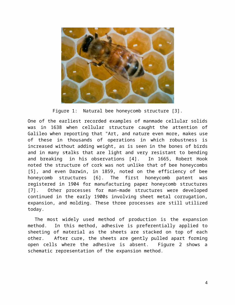
Cellular solids are those which contain portions of empty space and portions of solid material. The empty space can be either closed or open to the atmosphere and form ‘cells’ within the volume. Many cellular solids can be found in nature such as foams, sponges, and woods. Honeycomb structures are a specific type of cellular solid in which thin solid walls forming prismatic cells are nested together to fill a single plane [2]. As with many structural designs, honeycombs borrow their shape and name from nature; specifically the hexagonal honeycomb of bees as shown in Figure 1. Hexagonal shapes are often found in nature, like carbon structures, due to their high special efficiency, and it is not surprising that nature produces hexagonal honeycombs.

Figure 1: Natural bee honeycomb structure [3].

3

One of the earliest recorded examples of manmade cellular solids was in 1638 when cellular structure caught the attention of Galileo when reporting that "Art, and nature even more, makes use of these in thousands of operations in which robustness is increased without adding weight, as is seen in the bones of birds and in many stalks that are light and very resistant to bending and breaking” in his observations [4]. In 1665, Robert Hook noted the structure of cork was not unlike that of bee honeycombs [5], and even Darwin, in 1859, noted on the efficiency of bee honeycomb structures [6]. The first honeycomb patent was registered in 1904 for manufacturing paper honeycomb structures [7]. Other processes for man-made structures were developed continued in the early 1900s involving sheet metal corrugation, expansion, and molding. These three processes are still utilized today.

The most widely used method of production is the expansion method. In this method, adhesive is preferentially applied to sheeting of material as the sheets are stacked on top of each other. After cure, the sheets are gently pulled apart forming open cells where the adhesive is absent. Figure 2 shows a schematic representation of the expansion method.

Figure 2: Expansion process for honeycomb production [8].

For processing higher density honeycomb from thicker materials corrugation is the most common method of production. Sheets of metal are first corrugated to specified geometry. Then, adhesive is applied to the most external faces and the corrugated sheets are stacked so that they are aligned to form hexagonal cells. Figure 3 shows the corrugation production process. It should be noted that both the expansion and corrugated methods of production produce structures having double wall thickness where adhesive is applied which increases both weight and strength.

4

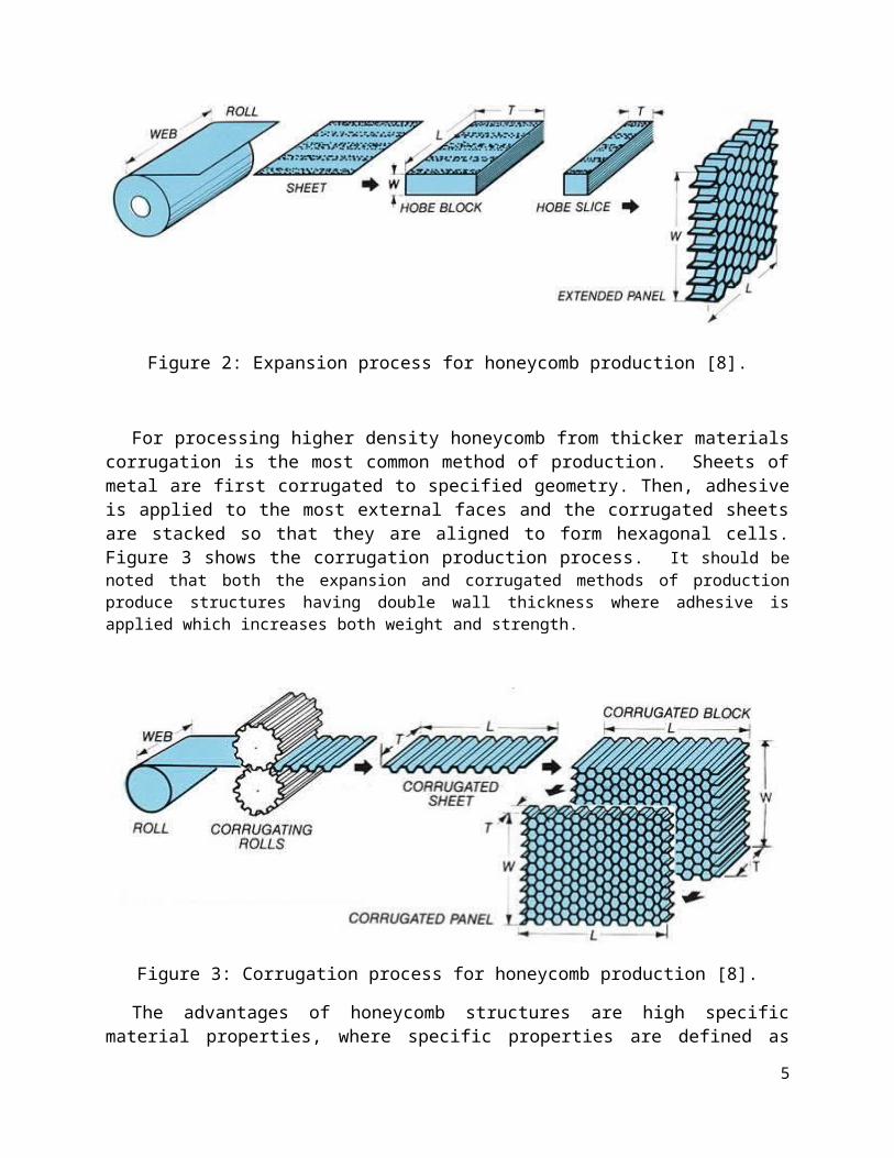
Figure 3: Corrugation process for honeycomb production [8].

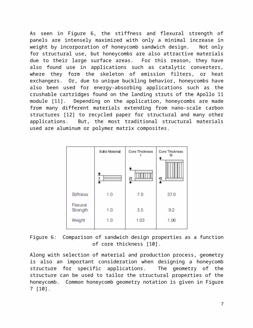
The advantages of honeycomb structures are high specific material properties, where specific properties are defined as characteristic values divided by a reference value (solid material properties, weight, mass, density, etc.). When honeycombs are sandwiched between facing panels, the resulting composite exhibits excellent specific strength and stiffness in bending as well as axial buckling resistance. For this reason, sandwich panel design is commonly used in aerospace and automotive industries where weight saving is crucial. Much like an I-beam, the facing plates resist most of the in-plane normal stresses, tension and compression; whereas, the honeycomb core resists shear stresses as shown in Figure 4 and 5 [9].

Figure 4: Honeycomb sandwich panel compared to I-beam [10].

5

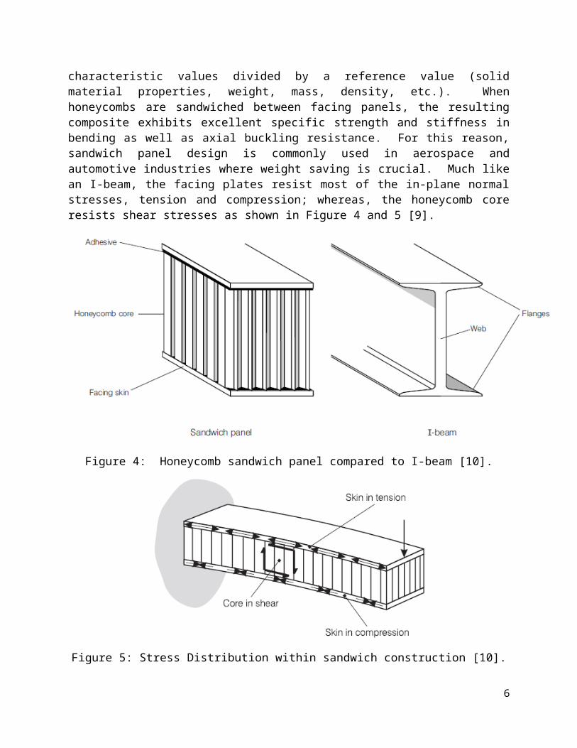
Figure 5: Stress Distribution within sandwich construction [10].

As seen in Figure 6, the stiffness and flexural strength of panels are intensely maximized with only a minimal increase in weight by incorporation of honeycomb sandwich design. Not only for structural use, but honeycombs are also attractive materials due to their large surface areas. For this reason, they have also found use in applications such as catalytic converters, where they form the skeleton of emission filters, or heat exchangers. Or, due to unique buckling behavior, honeycombs have also been used for energy-absorbing applications such as the crushable cartridges found on the landing struts of the Apollo 11 module [11]. Depending on the application, honeycombs are made from many different materials extending from nano-scale carbon structures [12] to recycled paper for structural and many other applications. But, the most traditional structural materials used are aluminum or polymer matrix composites.

Figure 6: Comparison of sandwich design properties as a function of core thickness [10].

Along with selection of material and production process, geometry is also an important consideration when designing a honeycomb structure for specific applications. The geometry of

6

1

23

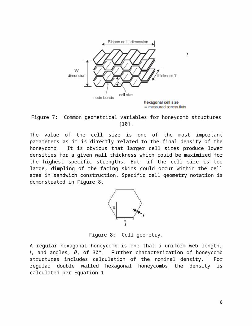
the structure can be used to tailor the structural properties of the honeycomb. Common honeycomb geometry notation is given in Figure 7 [10].

Figure 7: Common geometrical variables for honeycomb structures [10].

The value of the cell size is one of the most important parameters as it is directly related to the final density of the honeycomb. It is obvious that larger cell sizes produce lower densities for a given wall thickness which could be maximized for the highest specific strengths. But, if the cell size is too large, dimpling of the facing skins could occur within the cell area in sandwich construction. Specific cell geometry notation is demonstrated in Figure 8.

Figure 8: Cell geometry.

A regular hexagonal honeycomb is one that a uniform web length, l, and angles, θ, of 30°. Further characterization of honeycomb structures includes calculation of the nominal density. For regular double walled hexagonal honeycombs the density is calculated per Equation 1

ρ¿

ρs=

8( tl )3√3

(1)

where ρ* is the honeycomb density and ρs is the base material density. This relative density is an important factor and is commonly used to predict many material properties of the honeycomb structure.

b. Material Property Characterization

7

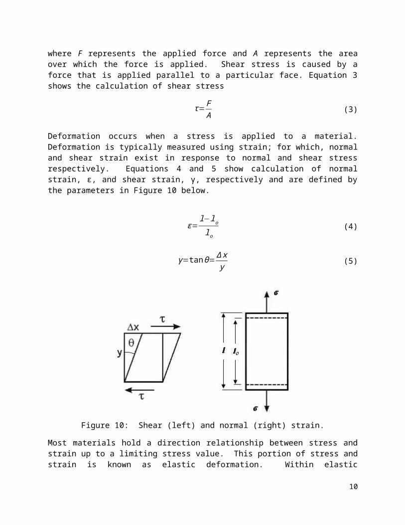
Consider Figure 9 below depicting the application of force to the faces of a simple cube.

Figure 9: Normal (left) and shear (right) stresses.

When characterizing mechanical properties of materials, it is important to be able to predict deformation of a material in response to a defined stress. In general, two types of stresses can be applied to a material, normal and shear. Normal stress is caused by a force that acts normal, or perpendicular, to a particular face. Equation 2 represents the calculation of normal stress

σ= FA (2)

where F represents the applied force and A represents the area over which the force is applied. Shear stress is caused by a force that is applied parallel to a particular face. Equation 3 shows the calculation of shear stress

τ= FA (3)

Deformation occurs when a stress is applied to a material. Deformation is typically measured using strain; for which, normal and shear strain exist in response to normal and shear stress respectively. Equations 4 and 5 show calculation of normal strain, ε, and shear strain, γ, respectively and are defined by the parameters in Figure 10 below.

ε=l−lolo

(4)

γ=tan θ=∆ xy (5)

8

Figure 10: Shear (left) and normal (right) strain.

Most materials hold a direction relationship between stress and strain up to a limiting stress value. This portion of stress and strain is known as elastic deformation. Within elastic deformation, the direct relationship is defined by a linear constant, specifically Young’s modulus, E, for normal stress/strain and shear modulus, G, for shear stress/strain. The equations governing elastic stress and strain are shown in Equations 6 and 7.

σ=εE (6)

τ=γG (7)

Elastic modulus values are used to compare the stiffness of different materials and structures. The higher the modulus, the stiffer the structure; or more simply, less deformation is experienced under loading. The properties of a particular honeycomb are often listed as the ratio of the honeycomb property to that of the base solid material. This study is a comparison of the out-of-plane material properties where these are defined as material properties referencing the open cell direction (thickness direction). For normal stress, out-of-plane stress is loading parallel to the cell direction; whereas for shear, out-of-plane stresses are applied perpendicular to the cell direction. It has been shown that relationship between the relative out-of-plane material properties can be closely predicted using the geometrical design or relative density properties of the honeycomb [13]. For the double-walled honeycombs in question, the relative Young’s modulus, E3*, has been shown to follow the trend as described below.

E3¿

E s≈ ρ

¿

ρs=2.67 % (8)

The relative shear modulus in the L-direction (G23*) for regular honeycombs has been shown to

fall within a range of values given by the cell geometrical relationships as follows [14].

9

32√3 ( tl )≤ G23

¿

Gs≤ 5

3√3 ( tl ) (9)

Or, later a more specific theoretical value was suggested by the relationship below using the upper and lower limits of Equation 9 [15].

G23¿ ≅G23lower

¿ +0.787 (G23upper¿ −G23lower

¿ ) (10)

For the W-direction, the relative shear modulus (G13*) has also been related to geometrical

values.

G13¿

G s=√3

3 ( tl ) (11)

c. Finite Element Analysis

FEA is a very powerful tool in understanding and designing structural components. The foundations of FEA lie in mathematical techniques developed in the early 1940s that evolved into the ‘finite element method’ in a paper written by R.W. Clough published in 1960 [16]. Gaining much attention across numerous fields of science and engineering from the 1940s to the 1970s, thermal/fluid dynamics and structural FEA was progressing steadily. Most studies of the new methods were focused in structural analysis, but by applying finite element methods to the Navier-Stokes equations, fluid and thermal analysis also became possible. Soon advances in structural FEA and the addition of more powerful computers allowed FEA to be applied more easily. Today, FEA is used in nearly every area of engineering, and it is not only an extremely important engineering tool but also an immense contributor to conserving design resources (e.g. iteratively predict without wasteful sample production and testing).

3. Experiment

a. ModelingThe models created for the purpose of this study were made to match the geometry and

specifications as close as possible to a commercially available honeycomb. The honeycomb used for modeling is made by Hexcel (Stamford, Connecticut) from Aluminum. The geometry of the model was matched to that used in a previous study performed to experimentally determine the material properties of the selected honeycomb [17].

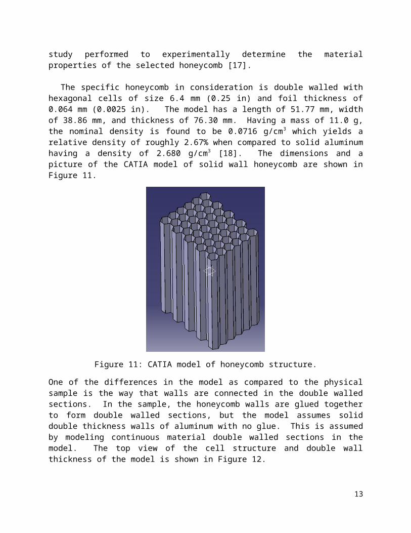
The specific honeycomb in consideration is double walled with hexagonal cells of size 6.4 mm (0.25 in) and foil thickness of 0.064 mm (0.0025 in). The model has a length of 51.77 mm, width of 38.86 mm, and thickness of 76.30 mm. Having a mass of 11.0 g, the nominal density is found to be 0.0716 g/cm3 which yields a relative density of roughly 2.67% when compared to solid aluminum having a density of 2.680 g/cm3 [18]. The dimensions and a picture of the CATIA model of solid wall honeycomb are shown in Figure 11.

10

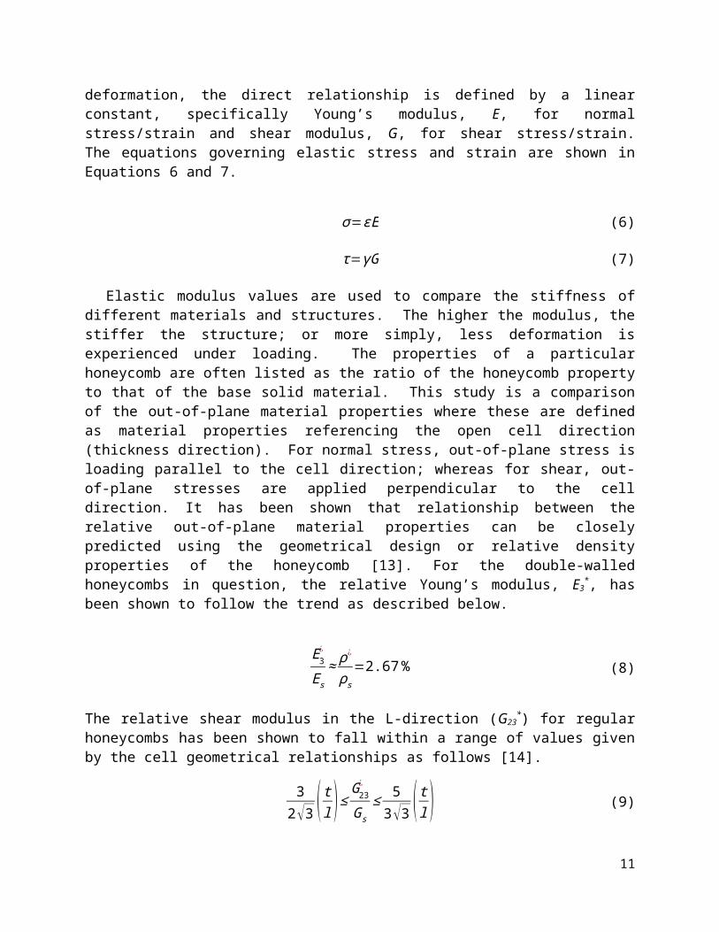
Figure 11: CATIA model of honeycomb structure.

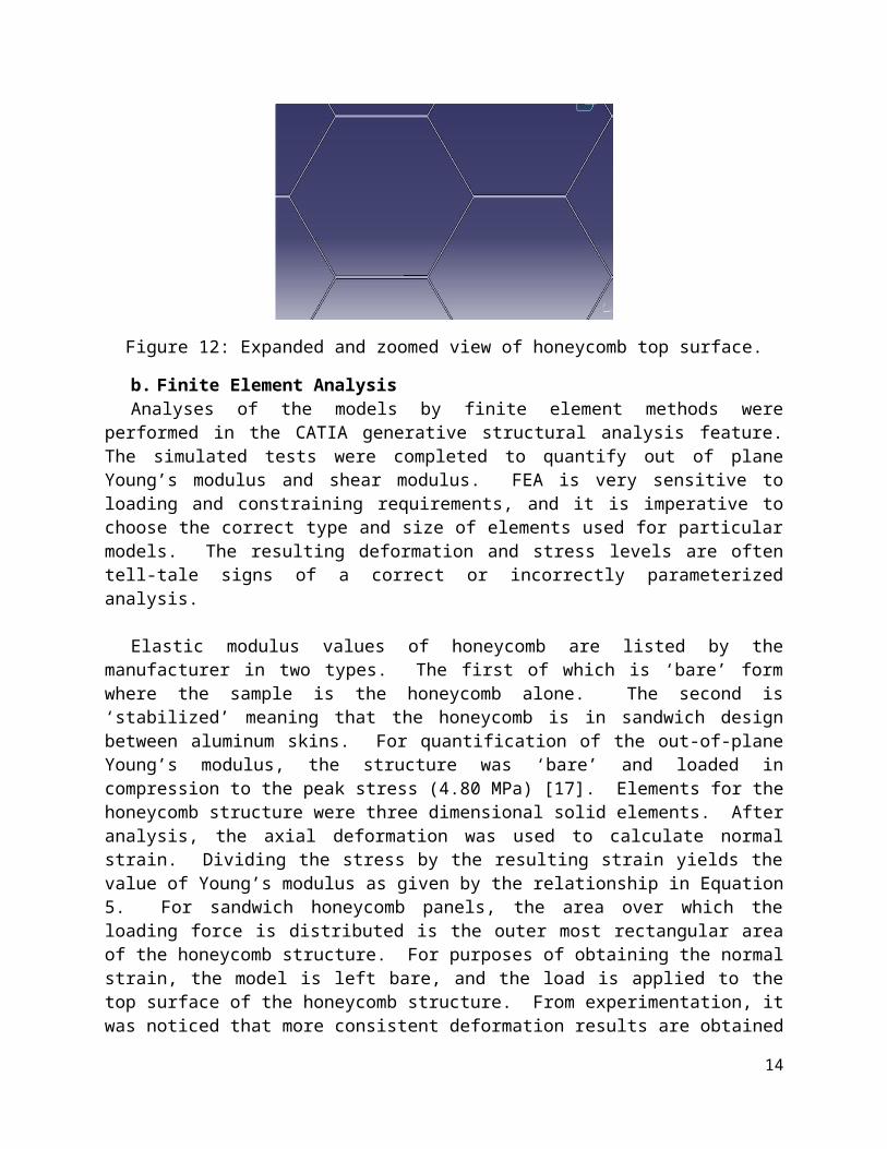
One of the differences in the model as compared to the physical sample is the way that walls are connected in the double walled sections. In the sample, the honeycomb walls are glued together to form double walled sections, but the model assumes solid double thickness walls of aluminum with no glue. This is assumed by modeling continuous material double walled sections in the model. The top view of the cell structure and double wall thickness of the model is shown in Figure 12.

Figure 12: Expanded and zoomed view of honeycomb top surface.

b. Finite Element AnalysisAnalyses of the models by finite element methods were performed in the CATIA generative

structural analysis feature. The simulated tests were completed to quantify out of plane Young’s modulus and shear modulus. FEA is very sensitive to loading and constraining requirements, and it is imperative to choose the correct type and size of elements used for particular models.

11

The resulting deformation and stress levels are often tell-tale signs of a correct or incorrectly parameterized analysis.

Elastic modulus values of honeycomb are listed by the manufacturer in two types. The first of which is ‘bare’ form where the sample is the honeycomb alone. The second is ‘stabilized’ meaning that the honeycomb is in sandwich design between aluminum skins. For quantification of the out-of-plane Young’s modulus, the structure was ‘bare’ and loaded in compression to the peak stress (4.80 MPa) [17]. Elements for the honeycomb structure were three dimensional solid elements. After analysis, the axial deformation was used to calculate normal strain. Dividing the stress by the resulting strain yields the value of Young’s modulus as given by the relationship in Equation 5. For sandwich honeycomb panels, the area over which the loading force is distributed is the outer most rectangular area of the honeycomb structure. For purposes of obtaining the normal strain, the model is left bare, and the load is applied to the top surface of the honeycomb structure. From experimentation, it was noticed that more consistent deformation results are obtained by applying loads as a surface force density (N/m2) instead of a distributed load. But, the stress applied to the rectangular surface cannot be applied to the top surface of the honeycomb because it is not the stress that is transferred to the honeycomb by the facing plate, but the force. Therefore, the loading of the top surface needs to be modified to apply an equivalent stress. This is done dividing the force transferred by the plate by the surface area of the honeycomb top surface. For a desired stress of 4.80 MPa, and a rectangular area of 2012 mm2, the equivalent stress is calculated below per Equation 6

σ R=FAR

(12)

F=σ R A R=( 4.80 x106 Pa ) ( 2.012 x10−3m2 ) (13)

F=9658N (14)

σ applied=FAH

= 9658 N53.39 x10−6m2 (15)

σ applied=1.809 x108Pa (16)

where σR is the desired stress, σapplied is the equivalent stress, AR is the rectangular area over which the desired stress is applied, AH is the top surface area of the honeycomb, and F is the transferred force. Lastly, when calculating Young’s modulus, the stress used for is the desired stress that would be distributed over the plate rectangular area.

The restraints for this experiment are relatively simple requiring just that the bottom face opposite of the loaded face resist translation in the loading direction. To allow for unhindered deformation in the loading direction, the two orthogonal directions are allowed to ‘slide’ on the imaginary surface at the bottom face. In CATIA, the restraint used is a ‘surface slider’. In order to use the surface sliding restraint, the body must also be iso-statically restrained. This restraint

12

is the equivalent to simply supporting the body in such a way that translation of the body is impossible without restraining internal translation or rotation. The iso-static restraint will choose three points to restrain by the 3-2-1 rule thereby restraining any singularity causing translation or rotation. Figure 13 shows an example of a body iso-statically restrained where the red arrows represent a restrained degree of freedom.

Figure 13: Iso-statically restrained body.

Without the iso-static restraint, the honeycomb would be free to translate along the ‘surface’ to infinity causing a singularity. This restraint must be used with caution so that the body is not over constrainded, but in this case, the body is still free to translate locally in the two orthogonal directions. Figure 14 shows the model restrained and loaded, just before starting the analysis.

Figure 14: Loaded and restrained model.

13

The measure peak stress value of out-of-plane compression is 4.80 MPa. From theory given by Ashby in Equation 7, and using know material data for 5052 aluminum [18] (although, the exact foil is not known), the calculated estimated modulus value is show below.

E¿

69.6GPa≈ 0.0712g /cm3

2.68g /cm3 (17)

E¿≈1.85GPa (18)

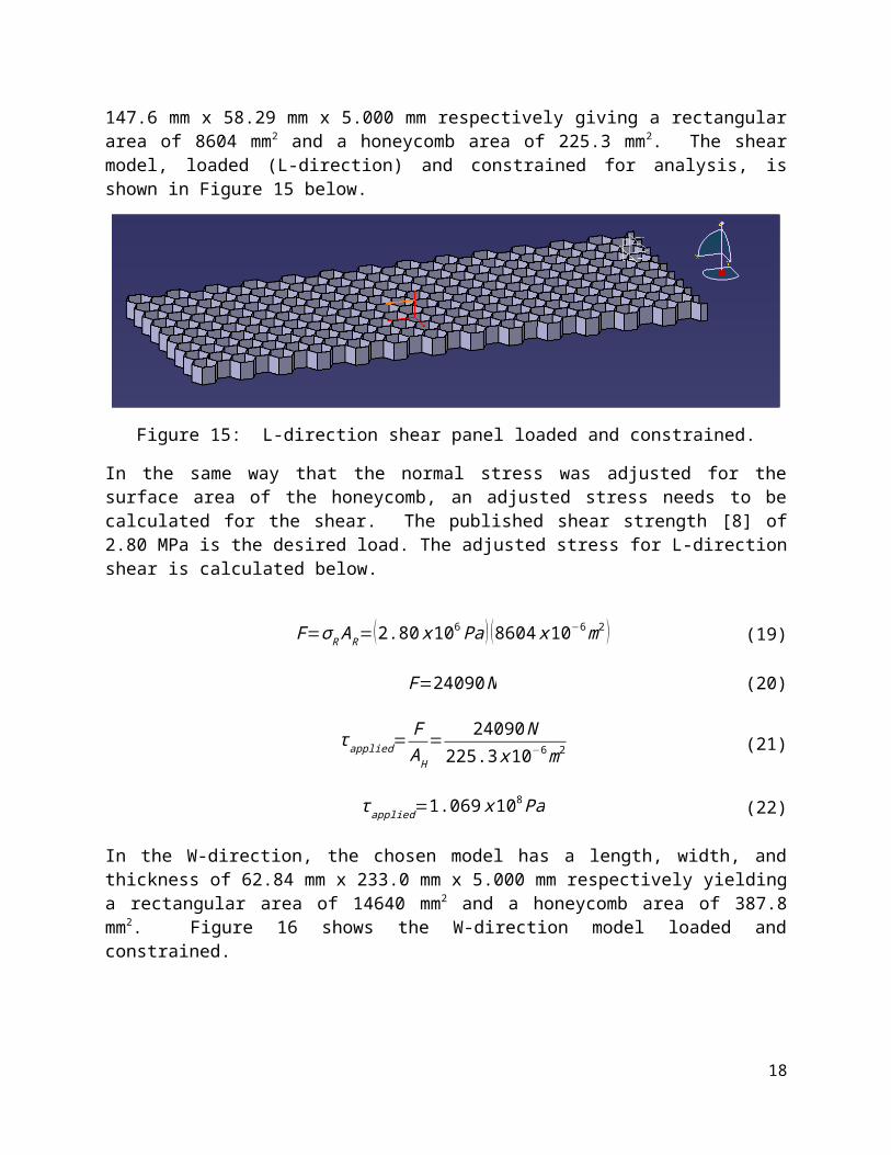
For analysis of the material properties under shear stress, the models were again left bare. For shear analysis, it was determined that the honeycomb outer dimensions needed to be adjusted which will be discussed in more detail later. In the L-direction, the chosen model has a length, width, and thickness of 147.6 mm x 58.29 mm x 5.000 mm respectively giving a rectangular area of 8604 mm2 and a honeycomb area of 225.3 mm2. The shear model, loaded (L-direction) and constrained for analysis, is shown in Figure 15 below.

Figure 15: L-direction shear panel loaded and constrained.

In the same way that the normal stress was adjusted for the surface area of the honeycomb, an adjusted stress needs to be calculated for the shear. The published shear strength [8] of 2.80 MPa is the desired load. The adjusted stress for L-direction shear is calculated below.

F=σ R A R=(2.80 x106Pa ) (8604 x 10−6m2 ) (19)

F=24090N (20)

τ applied=FAH

= 24090 N225.3 x10−6m2 (21)

τ applied=1.069 x108Pa (22)

In the W-direction, the chosen model has a length, width, and thickness of 62.84 mm x 233.0 mm x 5.000 mm respectively yielding a rectangular area of 14640 mm2 and a honeycomb area of 387.8 mm2. Figure 16 shows the W-direction model loaded and constrained.

14

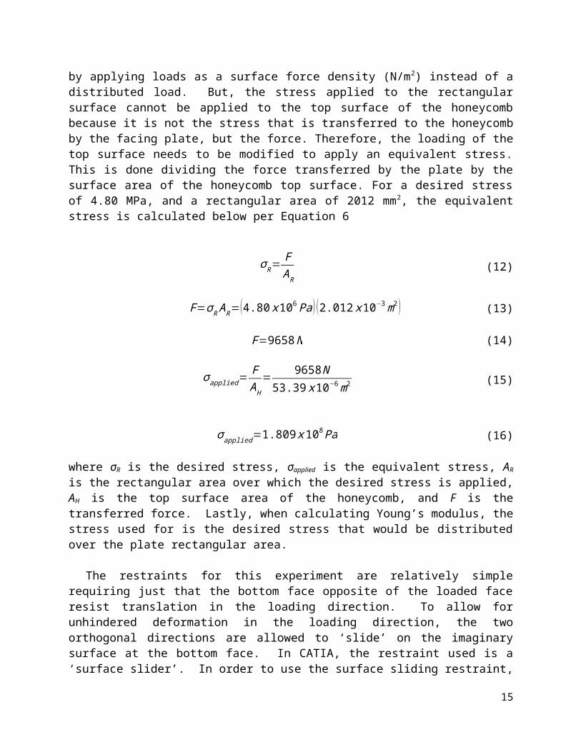
Figure 16: W-direction shear panel loaded and constrained

The published shear strength of 1.80 MPa is the desired load. The adjusted stress for W-direction shear is as follows.

F=σ R A R=(1.80 x106Pa ) (14640 x10−6m2 ) (23)

F=26,350 N (24)

τ applied=FAH

= 26350 N387.8 x10−6m2 (25)

τ applied=0.6795 x108Pa (26)

To allow the model to deform under shear the bottom face of the honeycomb structure needs to be simply supported such that all translation is restricted but free to rotate. The applied shear stress is then applied as a linear force density to the top face in either the L or W direction. In this case, the iso-static restraint may cause deformation issues due to the fact that the 3-point rule will restrict translation of the material above the simply supported bottom face. If the shear stress is in the same direction of the third corner of the iso-static restraint, then irregular deformation can occur. From Equation 8, a theoretical range of values for L-direction shear modulus is calculated below taking the shear modulus of aluminum as 26.54 GPa [18].

32√3 ( .064mm

3.739mm )≤ G23¿

26.54GPa ≤5

3√3 ( .064mm3.739mm ) (27)

393.4MPa≤G23¿ ≤437.1MPa (28)

From Equation 9, we receive a more specific theoretical value.

G23¿ ≅ 392.8MPa+0.787 (437.1MPa−392.8MPa ) (29)

G23¿ ≅ 427.7MPa (30)

15

From Equation 10, the theoretical W-direction shear modulus is calculated below.

G13¿

26.54GPa=√33 (0.064mm

3.739mm ) (31)

G13¿ =262.3MPa (32)

4. Results and Discussion

Figure 17 shows the deformed view of the model after compressive loading.

Figure 17: Deformed view after analysis.

It can be seen that the resulting deformation is consistent not creating any irregularities suggesting that the analysis was correctly loaded and constrained.

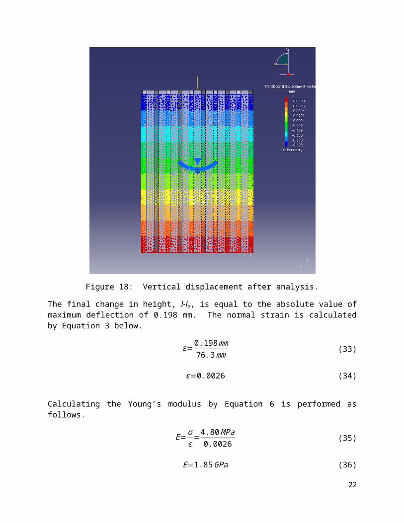
Figure 18 shows the displacement in the loading direction. Since the deformation is in the negative direction, displacement values are negative. The maximum deflection can be seen in blue on the top surface where the load is applied.

16

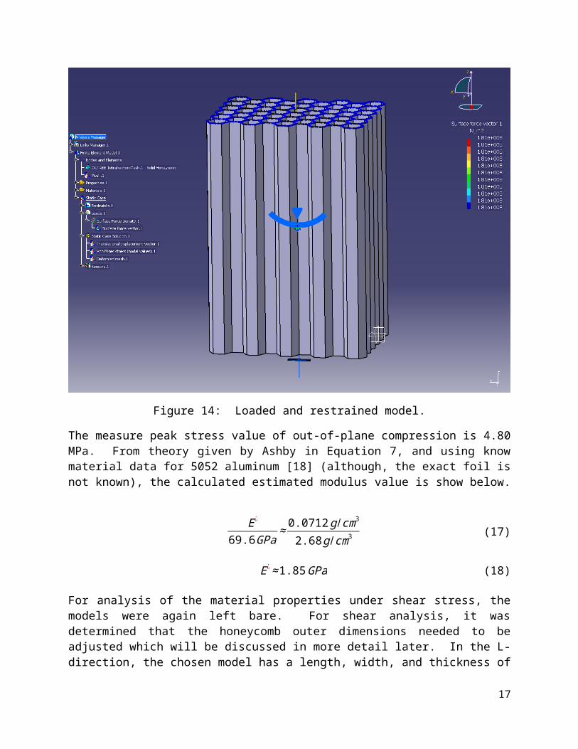
Figure 18: Vertical displacement after analysis.

The final change in height, l-lo, is equal to the absolute value of maximum deflection of 0.198 mm. The normal strain is calculated by Equation 3 below.

ε=0.198mm76.3mm (33)

ε=0.0026 (34)

Calculating the Young’s modulus by Equation 6 is performed as follows.

E=σε=4.80MPa

0.0026 (35)

E=1.85GPa (36)

It can be seen that the analyzed model matches the theoretical value of Young’s modulus. This result is an excellent qualification of FEA analysis of Young’s modulus for solid regular hexagonal honeycomb structures.

17

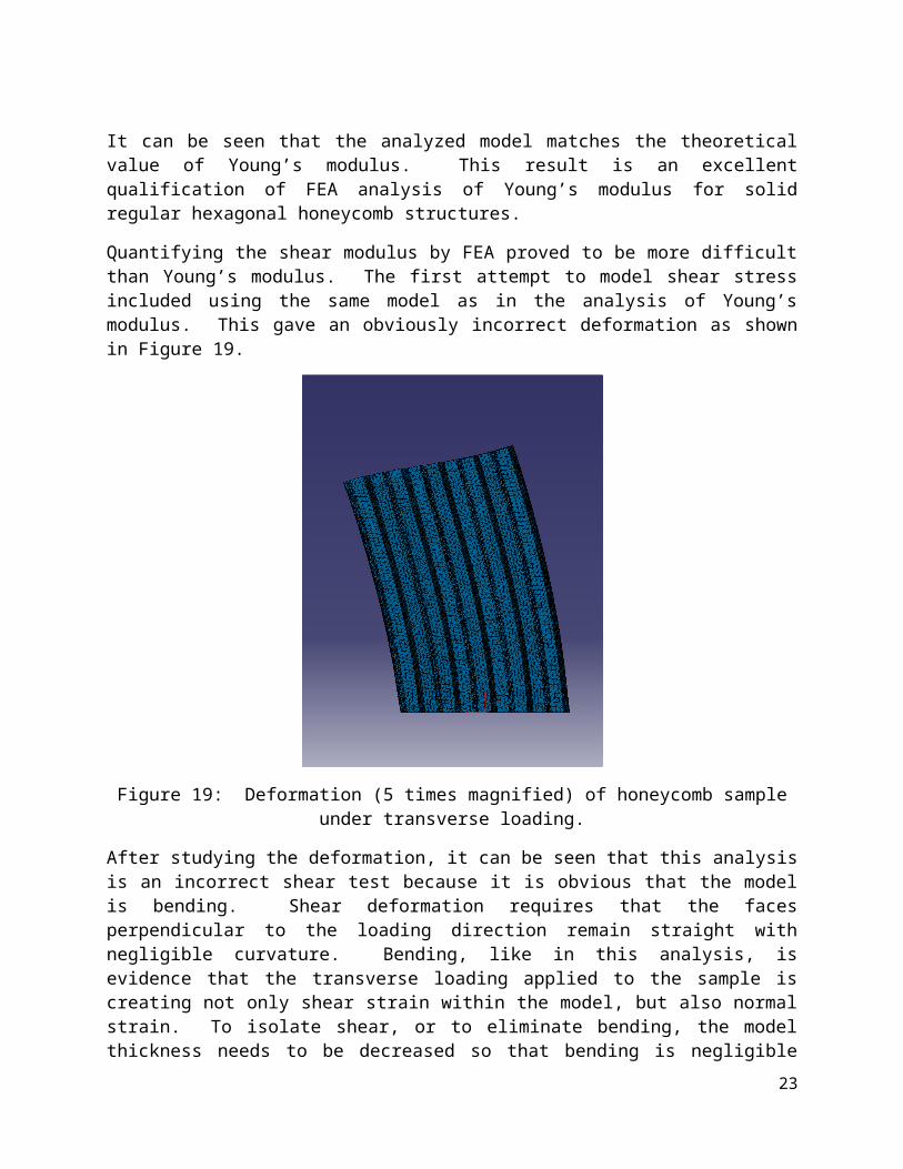
Quantifying the shear modulus by FEA proved to be more difficult than Young’s modulus. The first attempt to model shear stress included using the same model as in the analysis of Young’s modulus. This gave an obviously incorrect deformation as shown in Figure 19.

Figure 19: Deformation (5 times magnified) of honeycomb sample under transverse loading.

After studying the deformation, it can be seen that this analysis is an incorrect shear test because it is obvious that the model is bending. Shear deformation requires that the faces perpendicular to the loading direction remain straight with negligible curvature. Bending, like in this analysis, is evidence that the transverse loading applied to the sample is creating not only shear strain within the model, but also normal strain. To isolate shear, or to eliminate bending, the model thickness needs to be decreased so that bending is negligible compared to shear strain. If the thickness of this model is decreased to 5 mm (less than 10% of the original thickness), the sample no longer contains much material volume compared to the outer structure volume. This could yield inaccurate results, so to gain more accuracy, it was thought to increase the length and width as the thickness is decreased. In laboratory practice, thickness of honeycomb shear samples is traditionally at least one order of magnitude less than the dimension in the loading direction. To apply this principle to the model analysis, a shear panel (L-direction analysis) was modeled having the same foil thickness and cell size and dimensions of 295.3 mm x 116.58 mm x 10 mm. The resulting deformation of this model under shear was acceptable having negligible curvature. When the shear modulus was calculated from this test, it did not match the theoretical values, so the element size was decreased for more accuracy. With iterations of finer elements, the shear modulus result approached the theoretical range. Unfortunately, the decreased element size became impractical due to long computer computation times. To help decrease the computation times, all three dimensions were halved which still fulfilled the one order of magnitude criteria.

18

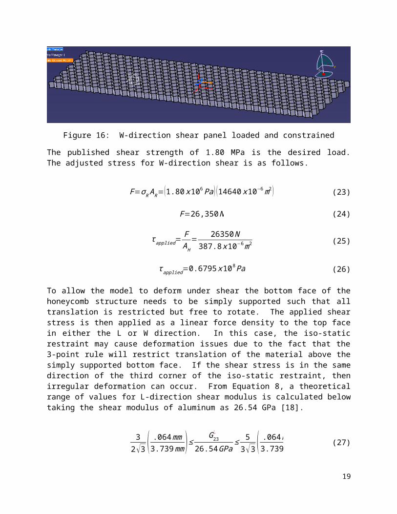
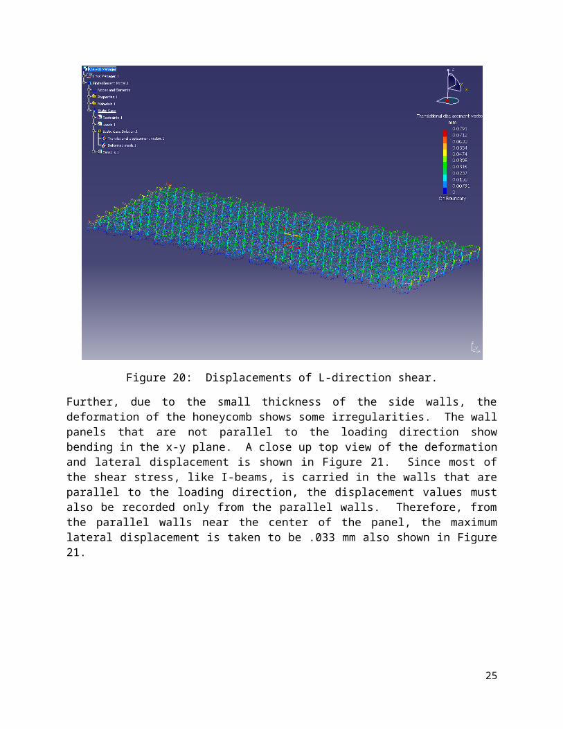
Figure 20 shows the displacement values (L-direction analysis) in the loading direction due to the applied shear stress. It can be seen that the displacements on the edges of the panel contain the extreme values of displacement and do not reflect pure shear deflection. Therefore, displacement values are taken from the center of the panel.

Figure 20: Displacements of L-direction shear.

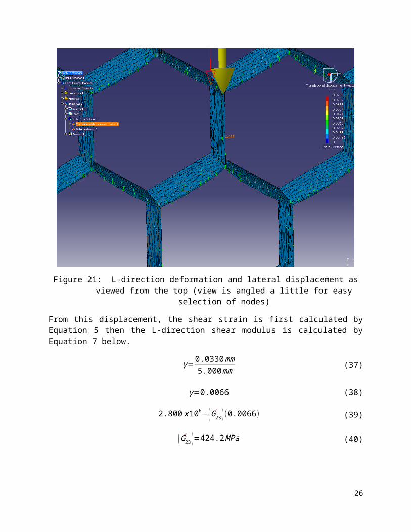
Further, due to the small thickness of the side walls, the deformation of the honeycomb shows some irregularities. The wall panels that are not parallel to the loading direction show bending in the x-y plane. A close up top view of the deformation and lateral displacement is shown in Figure 21. Since most of the shear stress, like I-beams, is carried in the walls that are parallel to the loading direction, the displacement values must also be recorded only from the parallel walls. Therefore, from the parallel walls near the center of the panel, the maximum lateral displacement is taken to be .033 mm also shown in Figure 21.

19

Figure 21: L-direction deformation and lateral displacement as viewed from the top (view is angled a little for easy selection of nodes)

From this displacement, the shear strain is first calculated by Equation 5 then the L-direction shear modulus is calculated by Equation 7 below.

γ=0.0330mm5.000mm (37)

γ=0.0066 (38)

2.800 x106=(G23¿ )(0.0066) (39)

(G23¿ )=424.2MPa (40)

This result falls within the theoretical range calculated for L-direction shear modulus and is 0.81% less than the specific theoretical value.

The same type of dimension adjustments were applied to the model for W-direction shear analysis except the longest length is assigned to the W-direction. Figure 22 shows the lateral displacements due to the applied shear stress.

20

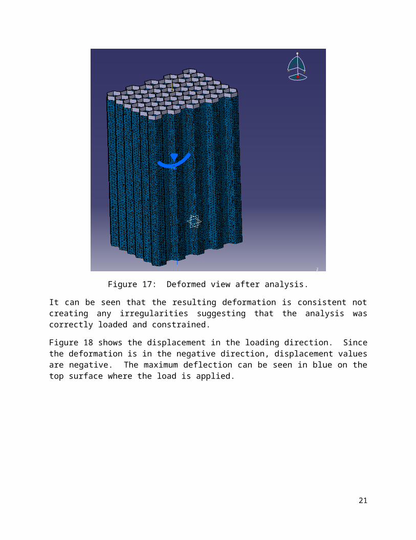
Figure 22: Displacements of W-direction shear.

When the model is loaded in the W-direction under shear, no specific wall is parallel to the loading direction; hence, the shear strength is decreased. As shown in Figure 23, all walls exhibit a certain amount of bending. For this, reason displacement values are taken at the intersection of walls. Displacements at these intersections are not all the same and give a small range of displacements also shown in Figure 23. The range of displacements for L-direction shear is taken as 0.0331 and 0.0340.

Figure 23: W-direction deformation and lateral displacement as viewed from the top (view is angled a little for easy selection of nodes)

21

From this displacement, the upper and lower limit shear strain is first calculated by Equation 5 then the limits of W-direction shear modulus are calculated by Equation 7 below.

γupper limit=0.0331mm5.000mm (41)

γupper limit=0.0066 (42)

1.800 x106=(G23¿ )(0.0066) (43)

(G13¿ )upper limit=271.9MPa (44)

γlower limit=0.0340mm5.000mm (45)

γlower limit=0.0068 (46)

1.800 x106=(G23¿ )(0.0068) (47)

(G13¿ )lower limit=264.7MPa (48)

The average value between these two results is 268.3 MPa which is 2.29 % of the theoretical W-direction value.

The final results of all analysis sets are compared to the theoretical values in Table 1.

Table 1: Results of FEA compared to theoretical values.

FEA (GPa) Theoretical (MPa) Error (%)E 1.85 1.85 0

G23 424.2 427.7 0.82G13 268.3 262.3 2.29

5. Conclusions

The possibility of using FEA methods for predicting material properties of solid wall honeycomb structures has been presented. The work accomplished in this study has qualified the application of FEA to honeycomb structures for prediction of elastic moduli. It has been shown that the FEA model accurately predicted Youngs modulus with less than 1 % difference and both L and W direction shear moduli with less than 3 % difference of theoretical values.

6. Future Work

22

Having established FEA within common honeycomb structures, the next step is to extend these capabilities to novel honeycomb designs. FEA will allow prediction of structural properties of new honeycombs even before production of physical samples. Such novel structures are truss-wall honeycombs like those presented by Dr. David Sypeck of Embry-Riddle Aeronautical University [17]. It is believed that these honeycombs could produce higher stiffness and strength properties per unit weight than the solid wall honeycomb structures. A truss wall honeycomb structure with similar cell size and density as the solid wall structure studied above is shown in Figure 24.

Figure 24: Truss wall honeycomb.

Preliminary study has begun on these structures. Geometrical and material constraints (i.e. cell size and honeycomb density) are used to determine the foil thickness and dimensions of trusses. Since corrugation methods would still be the best method for producing truss wall honeycombs, the model was also designed to have double wall characteristics. To yield a honeycomb having similar cell size and density, the foil thickness was set at 0.213 mm and the truss dimensions are 1.181 mm squares with spacing such that the cross-section of each member is a square (same length as the foil thickness). It should be noted that modeling the double wall trusses so that the honeycomb dimensions are correct has proven to be very difficult. The best result to date is a honeycomb having a mean cell size of 6.542 mm (6.613 mm when measured along W direction and 6.506 mm when measured in the two directions 60° offset from W direction) and a density of 0.0622 g/cm3 (+2.22 % and -13.1 % difference respectively).

23

Large surface areas and complex geometry make FEA more difficult of which truss wall honeycombs possess both. When attempting to conduct analysis on this model, computer memory and processing capabilities both became limiting factors. With these issues, analysis has only been performed with large mesh sizes that produce questionable and unverifiable results. One solution to this problem is to decrease the outer dimension of the honeycomb test model therefore decreasing the necessary computer power necessary allowing for smaller mesh sizes. But, when dimensions are decreased to workable sizes, the honeycomb properties are changed due to the fact that there are not enough cells to represent the full honeycomb structure. In fact, the structure is significantly less stiff when reduced to only a few cells. Figure 25 shows an attempt to analyze Youngs modulus of the truss wall honeycomb stabilized on the top and bottom. For correct analysis constraints, it was necessary to analyze these honeycombs stabilized; therefore, it would be necessary to compare these results with a stabilized solid honeycomb. But, this attempt was aborted due to lack of memory.

Figure 25: Stabilized analysis attempt.

Future work includes finding methods for increasing computer capabilities so that larger models having reasonable mesh sizes can be computed. Or, it may be necessary to use more powerful FEA systems such as NeiNASTRAN for future analysis of truss wall honeycomb structures.

7. References

1. Bitzer, T., Honeycomb Technology: Materials, Design, Manufacturing, Applications and Testing. 1997: Chapman and Hall.

2. Gibson, L.J.A., M.F., Cellular Solids: Structure and Properties. 1988, Oxford: Pergamon Press.3. Bee Honeycomb, 04/26/2011,

http://www.google.com/imgres?imgurl=http://www.wuway.com/graphics/bee%2520honeycomb.jpg&imgrefurl

4. Galilei, G., Discorsi e dimostrazioni matematiche, intorno á due nuoue scienze. 1638.

24

5. Hooke, R., Micrographia. 1665: London.6. Darwin, C., On the Origin of Species by Means of Natural Selection, J. Murray, Editor. 1859:

London.7. Budwig, D., Process of Manufaturing Honeycomb Paper, U.S.P. Office, Editor. 1904: United

States.8. Hexweb Honeycomb Attributes and Properties. 1999, Hexcel Composites.9. Campbell, F.C., Strucutral Composite Materials. 2010: ASM International.10. Hexweb Honeycomb Sandwich Design Technology. 2000, Hexcel Composites.11. Bryan, C. and Strasburger, W., Lunar Module Structures Handout LM-5. 1969, NASA.12. Angelucci, R., Boscolo, I., et al., Honeycomb arrays of carbon nanotubes in alumina templates for

field emission based devices and electron sources. Physica E: Low-dimensional Systems and Nanostructures, 2010. 42(5): p. 1469-1476.

13. Gibson, L.J.A., M.F., Cellular Solids: Structure and Properties. 1999: Cambridge University Press.14. Kelsey, S., Gellatly, R.A., and Clark, B.W., The Shear Modulus of Foil Honeycomb Cores: A

Theoretical and Experimental Investigation on Cores Used in Sandwich Construction, in Aircraft Engineering and AerospaceTechnology. 1958. p. 294-302.

15. Grediac, M., A finite element study of the transverse shear in honeycomb cores. International Journal of Solids and Structures, 1993. 30(13): p. 1777-1788.

16. Champion, E.R., Finite Element Analysis with Personal Computers. 1988: Marcel Dekker, Inc.17. Sypeck, D.J., Fabrication and Crushing Behavior of Highly Vented Honeycomb Structures, in

International Conference on Composites/Nano Engineering. 2010: Anchorage, Alsaka. p. 719-720.

18. Metallic Materials and Elements for Aerospace Vehicle Structures, in Military Handbook. 1998.

25

Acknowledgements

I would like to thank and recognize the help and opportunities offered to me during the completion of this work. First, to Dr. Zhao, department head and advisor of the Embry-Riddle graduate aeronautical engineering department, I would like to express my appreciation for the approval of this project. Also, I would like to recognize and thank the help of Dr. Radosta for advice and direction involving FEA intricacies and execution. Lastly, I would like to thank Dr. Sypeck, advising professor for this work, for allowing me this opportunity. Much appreciation is due to Dr. Sypeck for meeting regularly with me and offering not only much time but also advice on project direction and planning.

26