adrin huyer - ir.library.oregonstate.edu · parodia and pd. a study of wind, oceanic temperature...
TRANSCRIPT

AN ABSTRACT OF THE THESIS OF
FRANCISCO A. MEDINA for the degree of MASTER OF SCIENCE
(Name) (Degree)
in OCEANOGRAPHY (PHYSICAL) presented on 13 October 1978
(Major) (Date)
Title: A STUDY OF WIND. OCEANIC TEMPERATURE AND HYDROGRAPHY IN THE
UPWELLING AREA OFF PERU
Abstract approved:
Adrin Huyer
Observations of sea temperature, wind and hydrography obtained
during the three months' period of MAM 77 - CUEA experiment (JOINT-il)
along the C-line, near 15°S are described. Wind and temperature
observations made during March - May 1977 are compared to demonstrate
that a relationship exists.
Linear correlation analysis was performed on the temperature
data and on the alongshore component of wind and wind stress. Auto-
correlations and cross-correlations were computed for the temperature
and wind. These analyses show that the aiongshore fluctuations of
the wind are very similar at the different stations, and the wind at
each location was favorable for upwelling throughout the period of
measurements. Temperature fluctuations in the near-surface, the near-
shore and the near-bottom water over the shelf are coherent with
temperature changes at a depth of 150 - 280 m over the upper slope.
Temperature-wind analysis show that there is a good response of
the near-surface temperature to the wind force. The time lag between
Redacted for privacy

the wind and the near-surface temperature was about 24 hours nearshore;
the wind always led the temperature. Subsurface temperatures were
not as well correlated with the alongshore wind, both negative and
positive correlations were observed in this analysis, and the time
lag between the wind and temperature was variable; on a few occasions
the temperature led the wind.
Vertical sections of sigma-t and temperature indicate the
existence of conditions consistent with upwelling. Oscillation in
the wind with periods of several days caused significant changes in
the region inshore of 25 km.

A STUDY OF WIND, OCEANIC TEMPERATURE ANDHYDROGRAPHY IN THE UPWELLING AREA OFF PERU
Francisco A. Medina
A THESIS
submitted to
Oregon State University
in partial fulfillment of
the requirements for the
degree of
Master of Science
June 1979

APPROVED:
Research Assistant Professor af\Oceanographyin charge ofrriajor
Dean of School of Oceanography
Dean of Graduate School
Date thesis is presented 13 October 1978
Typed by Laina Reynolds Hardenburger for Francisco A. Medina
Redacted for privacy
Redacted for privacy
Redacted for privacy

This thesis is dedicated to my wife, Mercy. Herconcern, good humor, encouragement and supporthave played a very important part in this effort.
AC KNO WL EDGMENTS
I would like to express my appreciation to Dr. Adriana Huyer for
the constant encouragement and guidance which she extended to me
during the period of this research.
The author wishes to thank all members of the CUEA family at
Oregon State University who contributed in one way or another to the
outcome of this project. For his ideas and suggestions, I am grateful
of Dr. Dave Enfield,. Dr. Ken Brink made useful comments on the
coastal wind analysis. Mr. Bill Gilbert drafted the illustrations.
Most of the data used in this research were provided by the
Oregon State University. I especially want to thank Dr. Dave Halpern
of the University of Washington who provided the wind and temperature
data from the surface moorings. I also want to express my thanks to
LASPAU (Latin American Scholarship Program American University) and
the Escuela Superior Politecnica del Litoral (ESPOL) in Ecuador for
their support while working on my M.S. program.
Finally, I am indebted to Laina Hardenburger for her gracious
and efficient help in typing the drafts and final version of this
thesis.
Research for this thesis was supported under grants OCE 76-00594
and OCE 78-03381 from the Office for the International Decade of
Ocean Exploration, National Science Foundation. This is a contribu-
tion to the Coastal Upwelling Ecosystems Analysis Program0

TABLE OF CONTENTS
PageI. INTRODUCTION 1
The 1976-1977 Coastal Upwelling Experiment - JOINT II 2
II. DESCRIPTION OF DATA 6
Time Series from Moored Instruments 9
Temperature time series 9Wind observations 13Temperature-wind relationship 20
Hydrographic Observations 21
Variations of the hydrographic field 26
III. DATA ANALYSIS 28
Correlation Analysis 28Wind-Wind Correlations 29
Temperature-Temperature Correlations 30
Wind-Temperature Correlations 44
Correlations between temperature and 44wind stress at PSS
Correlation between near-surface temperature 52
and wind at the same locationCorrelation with near-shore and offshore wind 54
IV. SUMMARY AND CONCLUSIONS 57
V. REFERENCES 60
LIST OF FIGURESFigure Page
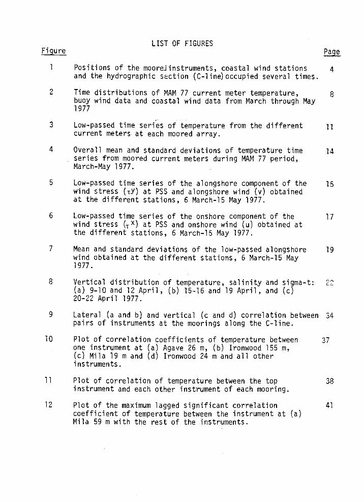
1 Positions of the moorej instruments, coastal wind stations 4and the hydrographic section (C-line)occupied several times.
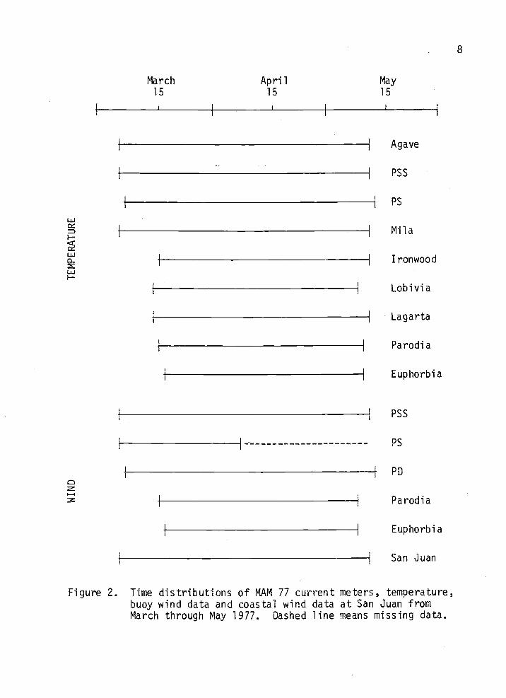
2 Time distributions of MAM 77 current meter temperature, 8buoy wind data and coastal wind data from March through May1977
3 Low-passed time series of temperature from the different 11
current meters at each moored array.
4 Overall mean and standard deviations of temperature time 14series from moored current meters during MAM 77 period,March-May 1977.
5 Low-passed time series of the alongshore component of the 15wind stress (TY) at PSS and alongshore wind (v) obtainedat the different stations, 6 March-15 May 1977.
6 Low-passed time series of the onshore component of the 17wind stress (IX) at PSS and onshore wind (u) obtained atthe different stations, 6 March-15 May 1977.
7 Mean and standard deviations of the low-passed alongshore 19wind obtained at the different stations, 6 March-15 May1977.
8 Vertical distribution of temperature, salinity and sigma-t: 22
(a) 9-10 and 12 April, (b) 15-16 and 19 April, and Cc)20-22 April 1977.
9 Lateral (a and b) and vertical (c and d) correlation between 34pairs of instruments at the moorings along the C-line.
10 Plot of correlation coefficients of temperature between 37one instrument at (a) Agave 26 m, (b) Ironwood 155 m,(c) Mila 19 m and (d) Ironwood 24 m and all otherinstruments.
11 Plot of correlation of temperature between the top 38instrument and each other instrument of each mooring.
12 Plot of the maximum lagged significant correlation 41
coefficient of temperature between the instrument at (a)Mila 59 m with the rest of the instruments.

Figure Page
13 Plot of the maximum lagged significant correlation 42
coefficient of temperature between one instrumentat (a) Agave 26 m, (b) Ironwood 155 m, (c) Mila 19 m,and (d) Ironwood 24 m with all other instruments.
14 Correlation between wind stress at PSS and temperature 49
from instruments along the C-Line.
15 Plots of (a) maximum lagged correlation between wind 54
stress (TY) arid temperature from current meters on themooring array along the C-line.

LIST OF TABLES
Table Page
1 Summary of positions, water depths and instruments 3
depths for instrument arrays in MAM 77.
2 Correlation coefficient at zero lag for onshore and 31
alongshore components of the windat different locations.
3 Simple linear regression coefficients between the "low 31
passe alongshore wind at PSS with other stations.
4 Correlation coefficients at zero lag between temperature 33records from different instruments along the C-line.
5 Maximum lagged correlation coefficients between temperature 39records from different instruments along the C-line.
6 Correlation coefficient between near-surface temperature 46at PSS, PS, Euphorbia and Parodia and the alongshore windstress at PSS.
7 Correlation coefficients between the alongshore wind 48stress at PSS and the temperature records from thesubsurface moorings along the C-line.
8 Correlation coefficient between the near-surface tempera- 53
ture records at PSS, PS, Euphorbia and Parodia and thealongshore wind at the same station.
9 Correlation coefficients between temperature at each 55
location and the alongshore component of the wind at PSS,Parodia and PD.

A STUDY OF WIND, OCEANIC TEMPERATURE ANDHYDROGRAPHY IN THE UPWELLING AREA OFF PERU
I. INTRODUCTION
Coastal upwelling is a dominant feature of the oceanographic
regime off the coast of Peru. Smith (1964) stated that it is along
the western coasts of the continents that the eastern boundary cur-
rents flow equatorward from high latitudes, and that it is there also
that the relative orientation of the predominant wind to the coastline
is suitable for sustained upwelling. This reasoning is applicable to
the area off Peru where the Peru current and a southerly wind are
prominent observed features.
Smith (1968) defined upwelling as an ascending motion of some
minimum duration and extent by which water from subsurface layers is
brought into the surface layer and is removed from the area of upwel-
ling by horizontal flow. In general, upwelling is the result of
divergence in the surface layer. Along the coast of Peru, a divergence,
hence coastal upwelling, occurs when the wind from the south causes an
Ekman tranposrt of surface waters away from the coast
This study describes wind and temperature data obtainedfrom
instrument arrays moored on the continental shelf and farther offshore
off Peru for the period from March through May 1977. Coastal wind
and hydrographic data are also described. The purpose of the present
work is to determine as well as possible the relationship between
wind and temperature fields for the three-month period. Also this
study is an attempt to use changes in wind and hydrographic data as
indicators of the oceanic phenomenon of upwelling.

The 1976-1977 Coastal Upwelling Experiment - JOINT-IL
The 1976-1977 interdisciplinary CUEA (Coastal Upwelling Ecosystems
Analysis) JOINT-LI experiment off Peru, has been the most recent study
carried out by the CUEA program, which has intensively studied other
areas of upwelling, i.e., Oregon and Northwest Africa (Huyer, 1976;
Halpern, 1976; Barton et al., 1977; Mittlestaedt, Pillsbury and Smith,
1975) to understand the characteristics that cause these areas to be
among the most biologically productive areas of the ocean.
The JOINT-Il experiment was a three phase field program. The
three intensive periods which JOINT-Il covered were March-May 1976
(MAM 76), July - October 1976 (JASON), and March-May 1977 (MAM 77).
The region studied extends about 660 kms in the alongshore direction:
from l6°S to about 1O°S, and about 200 km in the offshore direction.
Hydrographic surveys were made aboard ships from different U.S.
oceanographic institutions. Moored instruments were maintained
primarily by Oregon State University (OSU). In addition meteorologi-
cal buoys and near-surface current meters were installed by the NOAA
Pacific Marine Environmental Laboratory (PMEL).
This study utilizes the temperature data obtained from moored
current meters deployed along and near the
the MAM 77 phase field of JOINT-Il. Table
water depths and instrument depths for the
The locations of the moorings are shown in
During MAM 77, the continuous tempera
were supplemented by hydrographic sections
C-line (near l5°S) during
1 summarizes the positions,
different moorings examined.
Figure 1.
ture and wind measurements
along the C-line

Table I Summary of positions, water depths and instrunentdepths for instrument arrays in MAM 77. Onlyinstruments frorirwhich data were obtained arelisted M Meteorological buoy
Distance From WaterStation Position Shore (Kin) Depth (in) tnstrur'ent Depths (m)
Subsurface Moorings
Agave1 15°04 0'S 75°27 8'W 4 0 86 26 46 67 77
Mila1 15°06.O'S 75°30.8'W 12.0 121 19,39,59,80,100,115
Ironwood' 15°09 9'S 75°32 9'W 19 5 205 24,44,63 105,155 180
Lobivia' 15l1 5'S 75G34 3'W 24 0 580 58,83 183 283
Lagarta' 15°lO 0'S 75°36 O'W 24 0 620 92 115 214,512
Surface Moorings
Parodia 14°55 7'S 75°39 8W 10 5 12 M 3
Euphorbia' 15'31 2'S 75OO 8'W 7 0 123 M 3
P552 15°03 4'S 75°27 O'W 5 0 75 M 4 5 8,12 16
PS2 15°06 8'S 75°30 2'W 10 0 121 M 2 4 6 3 1 12,16 20 24
PD' 1°52 6'S 76°24 lW 125 D 26O '1
1 Oregon State University (OSU)
2 Pacif c arine Environrie'ital Laooraorj (?'4EL)

PDS
LCdbo Nozca
925 km
_____________I
00o
N /\Iosçna
76°W 75030 7c°
Figure 1. Positions of the moored instruments, coastal wind stations and thehydrographic sections (C-line) occupied several times.
150 S
5030'

5
(Figure 1) which were made from two ships: the R/V MELVILLE of
Scripps Institution of Oceanography and the R/V C. O'D. ISELIN of
University of Miami. This study utilizes only the hydrographic data
collected along the C-line by R/V ISELIN between 9 to 22 April 1977.

II. DESCRIPTION OF DATA
Current meter moorings were deployed along the C-line (near 15°S)
between March-May 1977. The moorings were of two kinds: surface and
subsurface taut-wire installations. The surface moorings were
deployed and recovered by Dr. Halpern's (Pacific Marine Environmental
Laboratory) group, CUEA Component 3. The mooring system used by this
group to measure wind, temperature and near-surface currents are
similar to the system used in previous expeditions (Halpern, Holbrook
and Reynolds, 1974) except that all current meters were VACM's
(Halpern, 1978). Measurements of the near-surface wind speed and
direction were made from surface buoys at 3 sites, called PSS, PS and
PD. The anemometer used to measure the wind was a VAWR type and its
calibration has been described in Halpern et al. (1974). Also,
temperature observations were obtained on the moorings at PSS and PS
on the continental shelf at a number of depths above 24.0 m.
Subsurface moorings were deployed and recovered by Oregon State
University (OSU). All these current meters were Aanderaa RCM4's
moored as describedby Pillsbury et al., (1974). Measurements of
the near surface wind were obtained at Parodia and Euphorbia (Table 1)
from meteorological buoys equipped with Aanderaa anemometers and data
loggers. Temperature data that are analyzed in this work are:
Parodia (3 m), and Euphorbia (3 m), and subsurface at Agave, Mila,
Ironwood, Lobivia, Lagarta and near surface at PSS and PS (Table 1).
In addition to wind measurements from buoys, the coastal
meteorological station at Pta. San Juan (15°2l2'S, 75°10.8'W),

7
installed and maintained by Dr. Stuartts group (CUEA Component 27),
provided us with an almost complete record of wind for this period.
In order to obtain a continuous coastal wind record, a gap of several
days in Stuart's record (Stuart, 1978) has been treated and filled
using a continuous wind record obtained during the same period at the
same location by the meteorological station maintained by Coorporacion
Peruana de Aviacion Civil (Medina, 1978). The time distribution of
the Aanderaa and VACM temperature data, the buoy winds and the coastal
wind at San Juan are shown in Figure 2.
Three different kinds of anemometers were used: Aanderaa (OSU)
data loggers, which recorded average speed and instantaneous
direction; vector averaging wind recorders (PMEL) which recorded
integrated values of the east and north components; and an MRI type
anemometer (Dr. Stuart's) which records speed and direction on a
strip chart recorder.
Two different types of temperature sensors (Aanderaa and VACM)
were used during MAM 77. Most of the temperature sensors on the
Aanderaa current meters used in MAM 77 as well as the temperature
sensors on the meteorological buoys at Parodia and Euphorbia were
calibrated before and after their use in JOINT-Il (Enfield, Smith
and Huyer, 1978). The resolutions of the temperature sensors of the
Aanderaa current meters and temperature sensors on meteorological
buoys are 0.02 and 0.08°C, respectively. For most of the current
meters employed in this study the post-calibration agreed well with
the pre-calibration except for Agave 46 m, and Mila 19 m which
LJ
I-
wwI-
March April May15 15 15
I I
I IAgave
I I
Pss
1
PS
I
Mila
I
Ironwood
Lobivia
ILagarta
I
Parodia
I
Euphorbia
I
PsS
II ----------------------- PS
I FPD
Parodia
Euphorbia
-i San Juan
Figure 2. Time distributions of MAM 77 current meters, temperature,buoy wind data and coastal wind data at San Juan fromMarch through May 1977. Dashed line means missing data.

disagreed. For the current meters which did not agree, the post-
calibration curve was used to process the data. Euphorbia and Parodia
temperature sensors showed good agreement on the calibration. To our
knowledge, the temperature sensors of the VACM's were not calibrated.
All the current meter measurements were quite nearshore and
within 25 km from the coast. Each Aanderaa current meter recorded
temperature at 20 or 30 minute intervals, while VACM types recorded
temperature at 15 minute intervals. Hourly data sets were formed and
these were filtered to eliminate tidal and higher frequencies by means
of a symmetrical low pass filter (half power at 0.6 cpd) spanning
121 hours. The filter-passed signals have nil amplitude at 1 cpd,
half amplitude at O7 cpd, and 95% amplitude at 0.5 cpd. Wind data
was rotated by 45° counterclockwise, the approximate general direction
of the coastline.
Time Series From Moored Instruments
Temperature time series. Figure 3 shows the low-passed time
series of temperature obtained from the different moorings. At the
nearshore surface mooring (PSS) the temperature variations between
5 m and 20 m were all in phase, while the temperature at the neighbor-
ing subsurface mooring (Agave) sometimes fluctuated out of phase
with the temperature above 20 m at PSS. Two other features are
observed in these low-passed time series of temperature recorded at
PSS and Agave: first, a fairly constant weak gradient is observed at
Agave from 26 to 77 m with some periods where the temperature is

isothermal between 67 and 77 m,
of the upper 16 m at PSS varies
.03°C m1 on April 11, when the
of uniformity in the temperatur
on several occasions during the
The plot of the low passed
10
and; second, the temperature gradient
between .16°C m1 on March 30 to about
temperature was very uniform. Periods
within the upper 16 m were observed
two months of observations.
time series of temperature at the
surface and subsurface midshelf moorings (PS and Mila) shows that the
temperature for the upper 24 m at PS is also decreasing and increasing
in phase as was observed at the nearshore PSS station. Despite the
fact that warmer temperatures were observed at PS (Le., 18.3°C at
2.5 m), the fluctuations for both PS and PSS, Agave and down to 80 m
at Mila show similar patterns. The vertical gradients of temperature
observed at PS and Mila are quite comparable to those measured at the
nearshore stations Agave and PSS; thus, for the same day, March 30,
the vertical gradient at PS was .1°C m1, decreasing to about
.009°C m1 on April 11.
The temperature time series at Ironwood, Lobivia and Lagarta
show that there exist two different regimes, above and below 120 m.
At Ironwood, the temperature variations above 120 m occur approxi-
mately in phase, especially in the last part of the record, i.e.
April and May. The water below 120 m seems to behave quite differently
from the water above 120 m. This is especially observed in the deeper
temperature time series for Ironwood (155 and 180 m), Lobivia (183 and
283 m) and Lagarta (214 m), which behave very similarly to each other,
but not to the shallower ones. This feature may perhaps be related
to the proximity of these measurements to the slope and shelf-break.

11
19.0
18.0 1 4.5 m PSS
18.0
17.0
1.o. 26
3.4.0 i. .19.0
m
.. .:17.0
6 Mcrch 1 April
Figure3. Low-passed time series of temperature from thedifferent current meters at each moored array.
AGAVE
May

18.0
17.0
16.0
15.0
14.0
13.0
12.0
16.0
15.0
14.0
13.0
12.0
il.0
10.0
18.0
15.0
14.0
13.0
12.0
IRON WOOD
24n,
9.0
8.0
7.0
8.0
17 Mcrch
Figure 3. Continued.
5/2
t May
12

13
The general properties of the temperature field measured at the
moored instruments is seen on Figure 4a, The mean temperature distri-
bution depicts isotherms (15 - 16°C) above 100 m rising upward toward
the coast as an indicator of the upwelling process which is in agree-
ment with Wyrtki (1963) who estimated upwelling off Peru to be limited
to the upper 100 m. Below 100 m the mean isotherms slope downward
toward the continental slope. The standard deviation of temperature
(Figure 4b) is highest near the surface and least between about 30 m
and 90 m.
Wind observations. Figures 5 and 6 show the plots of the low
passed alongshore Cv, northwestward) and onshore (u, northeastward)
component of the wind measured at the different locations during
MAM 77. The alongshore component (Figure 5) of the wind is northwest-
ward for almost the entire period of measurements, except for brief
calms and very short periods when the wind became southeastward, on
12 April at Parodia (P) and 21 April at Euphorbia CE). There seems
to be no significant difference in the mean alongshore wind between
stations PS, PSS, and PD (Brink, Halpern and Smith, 1978) or between
these and the meteorological station at San Juan (Figure 5). Parodia
and Euphorbia have the lowest mean alongshore wind through the period
of measurements, Figure 7 shows the mean and standard deviation of
the alongshore component of the wind for the different locations of
measurements. The San Juan wind has the highest mean ( = 5.8 m sec'),
while PSS has the most variability (V1= 2.0 m sec'),
The main feature observed in Figure 5 is that there is a similar-
ity in the fluctuations in the low passed alongshore wind measured

15°12 15°!0 15°0414
LoLa M A/6rn- 0
:_____:--- tOO
/4
200 E-
I/2fI
0
300
400
ITemperature (°C)Overall Mean
I52 t5°tO 5°O4
0/ March-May 1977 500 LoLa______________________I M A
/
/
0 <a2
20 km 0 02
04, 200
I
/ 300
4.)
I
0-I
Temperature (°CStandard Deviation
0 March-May 1977
20 km 0
Figure 4. Overall mean and standard deviations of temperature timeseries from moored current meters during MAN 77 period,March - May 1977.

2.0
-S
.0
9.0
6.0
3.0
.0
9.0
-St.)
6.0
. 3.0
.0
3
6
3
0
ALONGSHORE COMPONENTS 15
PSS
Pss
PS
March I Aprf May
Figure 5. Low-passed time series of the alongshore (northwestward)component of the wind stress (Y) at PSS and alongshore wind(v) obtained at the different stations, 6 March - 15 May 1977.

16
(J 3
0
-3
E
Figure 5. Continued.

ONSHORE-OFFSHORE COMPONENTS2.0
1
1.0
/- I_' r\ A - A
.0
3.0
.0 I I
3.0
.0 .
3.
17
PSs
flJ.l I_Pc _'t.# PP
-3. -
Figure 6. Low-passed time series of the onshore (northeastward) compo-nent of the wind stress (TX) at PSS and onshore wind (u)obtained at the different stations, 6 1'1arch 15 May 1977.

6r
3
3
-3
3
su
E
March I April I May
_3L.
Figure 6. Continued.
1I3

-
C
\'-
\\ 0 rn/Sec 5
N
750
5° 5
'505
750
Figure 7. Mean (top) and standard deviations (bottom) of the low-passedalongshore component of the wind obtained at the differentstations, 6 March - 15 May 1977.

20
over an area 125 km in the offshore and 50 m in the alongshore direc-
tion. Halpern (1978) has calculated the mean onshore-offshore gradient
of the alongshore wind. He obtained a value of 9.4 x l0 sec'
between PSS and PS and -7.3 x l0 sec1 between PS and PD. The
negative gradient obtained between PS and PD stations is the conse-
quence of larger mean wind at the offshore station PD (Figure 7). The
low passed onshore (u) component of the winds (Figure 6) did not show
the variability observed for the alongshore component.
Temperature-wind relationship. Zuta et al. (1975) observed that
temperature fluctuations over the area off San Juan have large
variations between 0 m and 20 m, but little variation between 50 m to
100 m. This agrees with the results presented in Figure 3.
Periods of strong favorable wind lasting 3 to 5 days were
separated by episodes of weak wind (Figure 5). During the periods of
intense upwelling as on 7-10 March and 10-14 April, the temperature
gradient of the upper 16 m at PSS and of the upper 24 m at PS is about
.03°C m1. With the decreasing of the southerly wind after these
periods, the upper layer at stations PSS and PS warmed considerably
and the temperature gradient increased to about .15°C m1 at station
PS, returning to temperature values near those measured before the
events.
The fluctuations of the nearshore temperature at PSS, PS and
Agave (Figure 3) are closely related to the changes in the alongshore
wind. Thus the appearance of colder (<l60°C) surface temperature
accompanied periods of northward wind stronger than 5 m sec1 and

21
warming periods occurred at times of weak wind. However, the apparent
response of the temperature field to the wind was not instantaneous.
A lag of about one day occurred between the onset of strong equator-
ward wind and a significant drop in temperature nearshore. A similar
lag was evident between the weakening of the wind and a rise of
temperature nearshore0
Hydrographic Observations
As a complement to the current meter observations, several
hydrographic sections were made along the C-line by the R/V MELVILLE
and the R/V C. O'D. ISELIN from early March to mid-May 1977. Station
separations ranged from 5 to 30 km. Observations were made with a
Geodyne Conductivity-Temperature-Depth (CTD) system and Niskin bottles
equipped with protected and unprotected thermometers0
As an early step in analyzing the CTD data, vertical sections of
temperature, salinity and sigma-t were drawn for every offshore line.
Examples are shown for the period 9-22 April 1977, surveyed by the
R/V ISELIN (Figure 8). The temperature data revealed evidence for
upwelling throughout the study period. Isotherms above 75 m slope
upward toward the coast and isotherms below 75 m slope downward
toward the continental slope. This divergence of isotherms is observed
within 30 km of the coast. The tendency of the isotherms to sink
shoreward at approximately 100 km from the coast is in agreement with
Zuta et al. (1975).

;;
7--
-
-
T (C)7 9-97
II
e5n
35./__5
347
346
345
II
250L/ 255
'-.- 260 _______________________260 /262
1100
-I-
L26.4' / 200
-26.6(
300L
68 ___________ 268__ 1I -400
270 I
270 /
/ SIGMA-I/
SIGMA-I soo
272I-
I I! I
'50 00 50 0 0 20 0
0/STANCE FROM SHORE (Rn,)
Figure 8a. Vertical distribution of temperature, salinityand sigma-t: 9-10 and 12 April 1977.
100
I4;-'3-----
/2
/
I
I 400
/
100C- L ne
2 April 977I
I R/V
5-
22

f09-8
I (CI
5-6 Ap 977
fl/V sehiv,
35. /.----------------------------
348
>34.8
348
---------- 34.7 -
26.8
27.0
/SALJNITY
25.9
260...
26.4
SIGMA-I
/6
I3
- -
T(C)C- LIM
9 Apr. 977
fl/V Is&m
262
SIGMA-I 5O0
0 40 20 0
0/STANCE FROM SHORE 1km)
Figure 8b. Vertical distribution of temperature, salinityand sigma-t: 15-16 and 19 April, 1977.
23

24
-J 300
T ICI - 500C - Une
7 ______________________________ 20-22 Ape, 77
P/V sCm,4500
I ii. I I I I I --i I 1 1
______L_.._________52__ ______350
348
300
346/SALINITYt246 250
j266/I I
220SIGMAT -soo
J. J J.1 I
50 too 50 0
DISTANCE FROM SHORE (kin)
Figure 8c. Vertical distribution of temperature, salinity andsigma-t: 20-22 April, 1977.

25
Barton (1977) has stated that the temperature field off Peru can
be taken as an accurate indicator of the density field. This conclu-
sion is verified in this study where temperature and sigma-t sections
both show similar distributions. The depth of the upwelling, based
upon the shoreward rise of isograms (temperature and sigma-t), is
estimated to be about 75 m which is the depth of the permanent thermo-
dine according to Wyrtki (1964). This estimate of the depth of
upwelling off Peru, is in agreement with Wyrtki (1963) who estimated
that upwelling off Peru is limited to the upper 100 m.
The sigma-t sections show that the 25.8 - 26.1 density band is
a good indicator of the upwelling process over the area off Peru.
That result differs from the 25.5 - 26.0 band commonly used for Oregon
(Pillsbury, 1972) and Northwest Africa (Ralpern, 1974). It is also
observed in Figure 8 that the isopycnals below 26.1, which was
approximately at 100 m, tended to sink shoreward resulting in a weak
density gradient between 75 m and 100 m. Enfield (1970) attributed
the sinking of the isograms to the presence of a coastal undercurrent.
The vertical distribution of salinity is also included in
Figure 8. In general, salinity decreases with depth from 35.1 o/oo
at the surface to 34.5% at depth of 500 m. Two prominent features
are observed on these sections: first, a relative minimum at approxi-
mately 100 m, and second, a relative maximum at about 175 m, both far
offshore. The existence of the minimum is attributed to a northward
flow (Wooster and Gilinartin, 1961) and the maximum observed below the
minimum is considered to be an indication of a poleward undercurrent.

26
Wyrtki (1963) stipulated that this undercurrent could be associated
with the Peru countercurrent. Apparently this result is not in agree-
ment with current observations obtained for MAM 77 (Brink, Allen and
Smith, 1978), where maximum mean poleward flow was observed at about
100 m, and only a weak poleward flow was observed below 200 m.
However, these current meter observations are far inshore of the region
where the minimum and maximum were observed.
Variations of the hydrographic field, The main features of the
hydrographic regime changes little during this sequence of observa-
tions. The isopycnals and isotherms generally rose and converged
toward the coast, and each of the sections was consistent with the
description of the hydrographic regime during the upwelling season
given by Enfield (1970) and by Zuta et al. (1975).
The similarity between the hydrographic sections was limited to
the interior of each section. Changes occurred in what appear to be
boundary layers near the surface, the shore and the bottom.
The first hydrographic section on 9-10 April (Figure 8a) clearly
shows the effect of upwelling. isopycnals rise toward the coast
gradually offshore and steeply as they approach the coast. The 26.0
sigma-t surface is at a depth of about 75 m at 75 km offshore and rises
to a minimum depth of about 25 m near the coast. The temperature
distribution resembles the sigma-t distributions, and the 16° isotherm
rises to the surface about 12 km from the coast. Farther offshore
than 100 km, the isotheniis are almost horizontal.
The wind began to decrease a little in intensity on 11 April and
its effects on the hydrography are apparent from the sections on

27
12 April (Figure 8b). The isopycnals have become less steeply inclined
nearshore. The 26.0 sigma-t surface which was observed on 9-10 April
at 25 m, is now found at 50 m depth. Only the 25.8 isopycnal is
observed at the surface very close to the coast. Even though the
distribution of temperatur does not show the changes observed in the
sigma-t distribution, it appears that an intrusion of warmer water
has squeezed the colder water (e.g. 16°C) against the coast. The
35.1 o/oo patches of salinity observed on the 9 April sections have
disappeared and only a narrower 35.1 0/00 patch is still observed at
about 50 km offshore.
From 12 April through 18 April the wind is variable in intensity.
The sections of 15-16 April resemble those of 12 April. On 18 April
the alongshore velocity of the wind is observed to reach values of
7.0 m sec1, The section of 19 April shows that the surface layer
nearshore became cooler and denser. Patches of 35.0 0/00 salinity
were observed at the surface to about 50 km offshore.
Large volumes of dense water (25.8 - 26.0 sigma-t band) were
observed over the shelf during all the sections examined0 Increased
isopycnal slopes were observed on 9-10 April, 18 April and 20-22
April, and we conclude that upwelling occurred during these periods.
Changes in the nearshore area were limited to the region less
than 20 km from the coast, and seemed to be related to the changes
in the surface layer. The isograms of temperature and sigma-t
diverged toward the shore. This characteristic is more apparent over
the shelf and break slope; this may be explained by the increase of
mixing in this region.

III. DATA ANALYSIS
Correlation Analysis
In order to make quantitative comparisons among the wind and
temperature time series, we computed auto and cross correlation
functions following Bendat and Piersol (1966).
The cross correlation function of two sets of random data
describes the general dependence of the values of one set of data on
the other. As a measure of time delays between sets of data, lagged
correlations are examined. The correlation coefficient, r, which
is dimensionless relates the change in y to the change in x was
computed as: (Crow et al., 1969).
- _xy
xy
where>and S, are the sample standard deviations of x and y,
respectively. Sxy is the covariance of x and y, which is defined as:
N
E
i=l (xj-X) (Yi-Y)xy N-1
Correlation coefficients at lags from 0 to 5 days at increments of
6 hours were computed between the various time series. For each cor-
relation the number of degrees of freedom was found using the method
suggested by Davis (1976), and the significance level was obtained
from Pearson and Hartley (1970, p. 146). For zero lag correlation,
the 95% confidence level (i.e., the probability that a given correla-
tion coefficient would be obtained from uncorrelated variables is less

29
than 0,05) is used as the test of significance. For lagged correla-
tion, the 99% confidence level was used as the test of significance.
The magnitudes of the critical correlation coefficients, rc, at
the 95% and 99% confidence levels varied from one pair of records to
another because of differences in the length of each time series.
The value of rc also varies because the integral scale T, which
estimates the time period between independent measurements, was
different for each pair of records.
The linear trend was removed from each time series before any of
the correlation computations were performed. The detrending was by
the least squares methods, The computations were performed on the
CDC 3300 computer of the OS-3 operating system. The correlations
were computed by a program which used the DETREND and CCORR sub-
routines in the OS-3 ARAND system (Ochs et al., 1973).
Wind-Wind Correlations
Comparison of the wind measurements made along the C-line and at
San Juan during MAM 77 (Figures 5 through 7) indicated that the along-
shore fluctuations of the wind are similar over the area of study.
Table 2 presents the values of correlation coefficients at zero lag
of the onshore and alongshore components of the wind at the different
stations. All values of correlations for alongshore components are
significant at the 99% confidence level (r > .43). This table shows
that the alongshore wind fluctuations at one location are correlated
with each other. No significant correlation values at 0 lag are
30
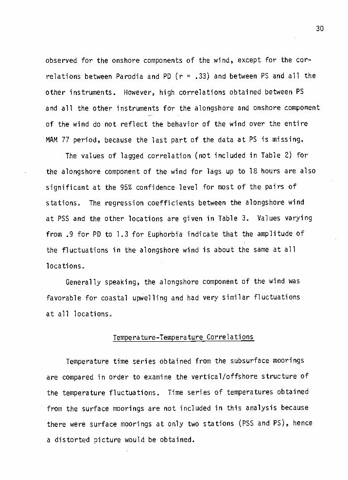
observed for the onshore components of the wind, except for the cor-
relations between Parodia and PD (r = .33) and between PS and all the
other instruments. However, high correlations obtained between PS
and all the other instruments for the alongshore and onshore component
of the wind do not reflect the behavior of the wind over the entire
MAM 77 period, because the last part of the data at PS is missing.
The values of lagged correlation (not included in Table 2) for
the alongshore component of the wind for lags up to 18 hours are also
significant at the 95% confidence level for most of the pairs of
stations. The regression coefficients between the alongshore wind
at PSS and the other locations are given in Table 3. Values varying
from .9 for PD to 1.3 for Euphorbia indicate that the amplitude of
the fluctuations in the alongshore wind is about the same at all
locations.
Generally speaking, the alongshore component of the wind was
favorable for coastal upwelling and had very similar fluctuations
at all locations.
Temperature-Temperature Correlations
Temperature time series obtained from the subsurface moorings
are compared in order to examine the vertical/offshore structure of
the temperature fluctuations. Time series of temperatures obtained
from the surface moorings are not included in this analysis because
there were surface moorings at only two stations (PSS and PS), hence
a distorted picture would be obtained.

31
Table 2. Correlation coefficients at zero lag for onshore (abovediagonal) and alongshore (below diagonal) components ofthe wind at different locations along and near the C-line.
Parodia Euphorbia San Juan PSS PS PD
Parodia - .06 -.28 .17 34* 33*
Euphorbia .80** - .09 .02 .31* - .22
San Juan .81** 77** - .23 .32* .13
PSS .89** .70** .80** - 73** .15
PS .92** .84** .87** .98** - 53**
PD .65** 47** 74** 76** 74** -
* Denotes correlation is significant at the 95% level.** Denotes correlation is significant at the 99% level.Italics are used for comparisons using data from PS because of itsmuch shorter record length.
Data intervals used in the comparisons are: PARODIA: 19 March-10 May(210 pts); EUPHORBIA: 22 March-10 May (199 pts); SAN JUAN: 6 March-13 May (273 pts); PSS: 6 March-13 May (273 pts); PS: 7 March-14April (156 pts); and PD: 9 March-15 May (270 pts).
Table 3. Simple linear regression coefficients between the "low pass"alongshore wind at PSS with the other stations
PS SJ P E PD
PSS 1.11 .94 .95 1.31 .90
Data intervals used in computations are the same as Table 2.
32
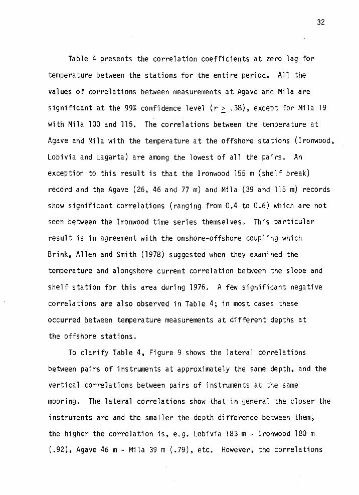
Table 4 presents the correlation coefficients at zero lag for
temperature between the stations for the entire period0 All the
values of correlations between measurements at Agave and Mila are
significant at the 99% confidence level (r > 38), except for Mila 19
with Mila 100 and 115. The correlations between the temperature at
Agave and Mila with the temperature at the offshore stations (Ironwood,
Lobivia and Lagarta) are among the lowest of all the pairs. An
exception to this result is that the Ironwood 155 m (shelf break)
record and the Agave (26, 46 and 77 m) and Mila (39 and 115 m) records
show significant correlations (ranging from 0.4 to 0.6) which are not
seen between the Ironwood time series themselves0 This particular
result is in agreement with the onshore-offshore coupling which
Brink, Allen and Smith (1978) suggested when they examined the
temperature and alongshore current correlation between the slope and
shelf station for this area during l976 A few significant negative
correlations are also observed in Table 4; in most cases these
occurred between temperature measurements at different depths at
the offshore stations0
To clarify Table 4, Figure 9 shows the lateral correlations
between pairs of instruments at approximately the same depth, and the
vertical correlations between pairs of instruments at the same
mooring. The lateral correlations show that in general the closer the
instruments are and the smaller the depth difference between them,
the higher the correlation is, e0g. Lobivia 183 m - Ironwood 180 m
(.92), Agave 46 m - Mila 39 m (.79), etc. However, the correlations

Table 4. Correlation coefficients at zero lag between temperature records from different instruments along the C-line.Agave Mila Ironwood Lobivia Lagarta
26 46 67 77 19 39 59 80 100 115 I 24 44 63 105 155 180 I 58 183 283 I 92 115 214 512
26 *92 *80 *75 *77 *82 *64 *50 *52 *54 .33 .08 -.00 .07 *54 *50 -.18 *43 .22 -.04 .06 .38 .35A
46 *91 *.82 *66 *79 *.78 *69 *.67 *58 .21 -.08 -.09 .08 *40 .28 -.29 .22 .01 -.07 .02 .15 .1867 *92 *56 *53 *.76 *.78 *73 *59 .05 -.23 -.08 .18 .29 .11 *_37 .07 -.17 -.02 .06 -.04 -.0477 *44 *55 *66 *.72 *.76 *.67 .04 -.18 -.06 .21 *40 .25 -.32 .23 -.03 -.02 .05 .06 .0219 *6] *41 *34 .28 .22 .63 .24 .01 -.14 -.06 .06 -.05 -.07 .22 -.09 -.11 .32 .3539 *.76 *50 *49 *46 .48 *53 *33 -.03 *40 .27 .20 .14 .11 .11 .11 .17 .11
*.88 *.72 *49 .01 -.01 .11 .16 .20 -.05 -.14 03 *.40 .04 .10 -.33 -.23Mila80 *87 *52 .02 -.27 -.11 .17 .04 -.13 -.26 -.09 *37 -.06 -.01 -.29 -.24
100 *49 .02 -.18 -.04 .28 .30 .09 -.18 .l3 -.12 .07 .08 -.09 -.15115 .14 .05 .08 .31 *60 *.38 -.02 *40 .22 *.83 .22 .16 .03
*61 Q5 *3p .02 .12 .20 ...67 .26 .18 .16 .31 .31*35 *.29 *3] *3] *65 .16 .26 .04 .07 .17 .10
63 * 34 * 26 04 * 55 - 02 03 * 62 * 57 - 16 -25Ironwood105 .22 -.18 -.15 -.03 -.17 *79 *78 -.28 *_5Q155 *78 .26 *77 .22 .25 *33 .29 .02180 OATA INTERVAL .23 *.92 .40 -.09 -.05 *.65 *4]58
.16 .11 .29 .28 .01 -.12Lobivia 183 AGAVE: 6 March - 13 May (272 pts) .33 -.03 .03 *59 35
283 MILA: 7 March - 13 May (270 pts) *.77*.48_QL_-.Q.89 -.22 *..4992 IRONWOOD: 18 March - 13 May (227 pts)
115 LOBIVIA: 17 March - 10 May (217 pts) -.29 *_53Lagarta214 LAGARTA: 17 March - 13 May (229 pts) *52512
Coefficients in italics are not significant at the 95% level. An asterisk indicates the correlation is significant at the 99% level.
()

IY2 l510 I50 504LoLa M A
.-63-77------- /I
,//--.?6--_... I
(0)
.77z.42,..
_65
00
200
00
400
500
15?IZ I5l0' u50
LoLa I M A.-33/
(b)
7/
40 20 km 0 40 20 km 0
Cc)
iT:''1
t1j.62/
00
200
300
4CC
500
Itl2 l5'I0 504LoLo M A
3o28.22T:;iCd)
34
U
m
100
200
300
400
500
U
m
'Co
200
300
400
500
40 20 km 0 40 20 km 0
Figure 9. Lateral (a and b) and vertical (c and d) correlationbetween pairs of instruments at the moorings alongthe C-line.

35
between Mila arid Agave are higher than between the offshore stations,
despite the greater distance between them. Also, there is essentially
no correlation between the mid-depth Mila (59 and 100 m) and Ironwood
(63 and 105 m) instruments. Except for these two pairs, all lateral
correlations between neighboring moorings are significant, but there
is no significant lateral correlation between moorings farther apart,
Le. between Ironwood and Agave or between Lobivia or Lagarta and
Mila (Figure 9b).
Figure 9c shows the vertical correlations between adjacent
instruments on the same moorings treating Lobivia and Lagarta together
as a single mooring, as well as separately. Generally speaking, the
temperature records from adjacent instruments are significantly cor-
related, although this is not observed at Lobivia, or at the inter-
mediate depths at Ironwood0 Only at Agave is the top temperature
record positively correlated with the deepest one (Figure 9d).
Records with similar vertical separations (about 50 m) at the other
moorings are riot significantly correlated (Figure 9d). There is weak
negative correlation between the 92 m and 512 m instruments at
Lagarta, but Figure 3 indicates that this negative correlation is due
to very low frequency trends: warming at 92 m and 115 m and cooling
at 512 m from the beginning of the record until about 10 April 1977,
and then cooling at 92 and 115 m and warming at 512 m until the end
of the record.
To see to what extent the temperature fluctuations at the differ-
ent instruments act together, Figure 10 shows the value of correlation

36
coefficients obtained between the shal lowest instruments at Agave,
Mila and Ironwood and Ironwood 155 and all the other instruments.
The significant correlation coefficients (r > .30) between Agave 26
and other instruments (Figure lOa) show that the fluctuations over
the inner shelf are correlated with those in the near-bottom water in
the vicinity of the shelf-break. Also the changes in the near bottom
water over the shelf are coherent with temperature changes at a depth
of 150 - 250 m offshore. This coherence is more clearly shown in
Figure lOb, which shows the correlation coefficients between Ironwood
155 m and the rest of the instruments. This result again emphasizes
the strong onshore-offshore coupling already mentioned for the correla-
tion between Ironwood 155 m with the shallower instruments at Agave
and Mila (Table 4).
Figures lOc and lOd are the plots of the correlations between
Mila 19 and Ironwood 24 with all other instruments. Those figures
suggest that besides the onshore-offshore coupling mentioned before,
the near surface temperature fluctuation seems to be coherent over
the shelf. Figure 11 shows the vertical correlations between the top
instrument and each other instrument of each mooring. The vertical
correlation decreases with increasing water depth and distance from
shore.
Table 5 presents the maximum lagged values of correlation
coefficients for temperature between all instruments. Only values
significant at the 99% confidence level and their corresponding lag
are included. A comparison between the zero lag correlation and

(a)
15°12 1510 I506 I5O4
LoLa I M A
\JIIll -
Correlation with// qove26/ / March-May 1977
4
U
m
100
200
300
40 20 km 0
15'IZ 1510 I5O I504
LoLa I M A
(c) x
x
x )(
x
x
Correlation with
/ Mila 19
400
500
U
m
100
200
300
400
500
37
1512 510 I5O6 I5O4
LoLa M A
(b)0.3x-..
0Jx
<03x
/ Correlation withj Ironwood 155
K
40 20 km 0
I592 5I0 I506 I504
LoLa I M A
(d)<.4
x
K X
x
K
Correlation with
/ Ironwood 24'I
Figure 10. Plot of correlation coefficients of temperature betweenone instrument (designated by a star) at (a) Agave 26 m,
(b) Ironwood 155 m, (c) Mila 19 m, and (d) Ironwood 24 m
and all other instruments. Instruments marked with an
X do not have significant correlation at the 95% level.
0
rn
100
200
300
400
500
U
m
100
200
300
400
500

-1.0 0 1.0 0I
I -r
50 Lobivk
I00Iz
Lagaric
200
300
4..
500
Ironwood
1.0 0.5 1.0 0-,
I
ii li/a
1.0-0m
-'100
A gave
Figure 11. Plot of correlation of temperature between the topinstrument (designated by a star) and each otherinstrument of each mooring.

Table 5. Maximum lagged correlation coefficients (above diagonal) between temperature records from different instruments along theC-line, March - May 1977, and the lag (below diagonal) at which the maximum occurs.
Agave
Mi la
I ronwoo
Lobibia
Lagarta
Agave Mila Ironwood Lobivia Lagarta
26 46 67 77 19 39 59 80 100 115 24 44 63 105 155 180 58 183 283 92 115 214 512
26 .92 .80 .75 .77 .82 .64 .50 .52 .54 .34 - - - .56 .54 - .51 - - - - -
46 0 .91 .82 .66 .79 .78 .69 .67 .58 .36 - - - .44 .34 - - - - - - -
67 0 0 .92 .57 .64 .76 .78 .74 .60 - - - - .41 - - - - - - - -
77 0 0 0 .46 .58 .66 .72 .77 .70 - - - - .47 .39 - - - - - - -
19 0 0 -1 -2 .67 .41 .35 - - .63 - - - - - - - - - - - .53
39 0 0 -1 -2 0 .76 .50 .50 .47 .48 .53 - - .40 - - - - - - - -
59 0 0 0 0 0 0 .88 .72 .49 - - .41 - - - - -.51 -.54 - - -.66 -
80 0 0 0 0 0 0 0 .87 .52 - - - - - -.54, - -.60 -.52 - - -.66 -
100 0 0 -1 -1 - 0 0 0 .49 - - - - .42 - - - - - - -.62 -.49
115 0 0 -1 -1 - 0 0 0 0 - - - - .69 .53 - .49 - .83 - - -
24 -1 -9 - - 0 0 - - - - .61 - -.36 - - - - - - - - -
44 - - - - - 0 - - - - 0 .36 - .34 - .65 ;-
63 - - - - - - 16 - - - - -1 .43 - - .59 - - .64 .57 - -
105 - - - - - - - - - - -2 - 3 .44 - - - - .80 .78 - -.51
155 -1 2 3 3 - 0 - - -5 3 - 2 - -10 .81 - .77 - - - - -
18023 - 4 - - - 8 --4 - - - - 1 - .92 - - - .65 -
58 - - - - - - - - - - - 0 0 - - - - - - - - -
1833- - - - - 8 8 --3 - - - - 0 0 - - - - .59 -
283 - - - - - - 8 8 - - - - - - - - - - - - . 79 -
92 - - - - - - - - - 0 - - -1 1 - - - - - . - -
115-- - - - - - - - - 0 0 - -: - - - U - -
214 - - - - - - 8 8 10 - - - - - - 0 - -1 -1 - - .63
512 - - - - -18 - - - 11 - - - - 0 - - - - - - - -1
Only correlation coefficients significantly different from zero at the 99% level are included. The lags are multiples of six hours,and are positive when the instrument nearer shore (or nearer the surface, if at the same location) leads. Data intervals are thesame as in Table 4.
c.)

40
lagged values (Tables 4 and 5) shows that the difference between the
zero lag and the maximum lagged correlation between Agave and Mila is
less than .03, and hence the lag is not significantly different from
zero. The lag (if any) for these nearshore stations varies from 6
to 12 hours, Mila leading' Agave. A similar result is observed for
the correlations between Agave and Ironwood, where the difference
between the zero lag and the lagged correlations did not exceed .07.
The lag varies from 6 to 54 hours, and in most cases Agave leads
Ironwood. Also, as was observed for zero lag, no significant correla-
tion at the 99% confidence level is observed between Agave and Lobivia
or Lagarta. The exception to this, as was observed for zero lag, is
found between Agave 26 and Lobivia 183.
Zero and lagged correlation coefficients between Mila and Iron-
wood showed almost no difference. The exception to this, is observed
between Mila 80 m and Ironwood 180 m which are uncorrelated at zero
lag but have a significant negative lagged correlation with Mila
leading. Significant negative correlations are also found between
the instruments at mid-depth at Mila (59 m, 80 m, and 100 m) and the
instruments at Lobivia and Lagarta from 180 to 512 m. Figure 12 shows
the plot of the maximum lagged correlation coefficient, and the lags,
between the instrument at Mila 59 and all other instruments. From
this figure it looks as if the temperature measured at depths of
about 150 - 200 m over the shelf break and upper slope is fluctuating
in the opposite direction than at mid-depth at Mila.
Figure 13 shows the distribution of the maximum lagged correla-
tion coefficients and the lags between all instruments and the

l5i2 5iO' 1506 5'04'
LoLa I M A
11i
!
J'Lagged Correlation
I with Mlo 59'C
20 km 0
0
m
I00
200
300
400
00
40
5'12' I5'IO I5O6' 1504'
LoLa I M A
'C'0
'C 0'C
'16 * 0.
'C
'8 'C
8
8
Lags,. Mila 59
20 km 0
Figure 12. Plot of the maximum lagged significant correlationcoefficient of temperature between the instrumentdesignated by a star at Mila 59 m and the otherinstruments. The lags (multiples of six hours)positive when Mila 59 leads are also shown. Instruments
marked with an X do not have significant correlation atthe 95% level.
shallowest instruments at Agave, Mila and Ironwood and Ironwood 155.
Although larger values are observed for lagged correlation than for
zero lag correlation, the distributions are very similar to those for
zero lag (Figure 10). The random distributions of the lags, which
range -60 to +12 hours (Figure 13), suggest that the lagged
correlations may not be very reliable.
41
0
m
00
500

l5t2 15°IO 1506' 1504
LoLa M A
(a)
x
Lagged Correlationj with Agave 26
x
40 20 km 0
I5I2 1510 506 15'04
LoLo M A
j Lagged Correlation
Jwith Ironwood 155
xf
0
In
00
200
300
400
500
0
m
00
200
300
400
500
1512 15010 15006 i5O4
LoLa I M A
*1g ;'o 0
xX
X
.3 '2
x
x
Logs, Agave 26
40 20 km 0
I5l2' 1510 1506 I504
LoLa I M A
x 0-I
x
x
'I
x
/Logs, Ironwood 155
x
40 20 km 0 40 20 km 0
Figure 13. Plot of the maximum lagged significant correlationcoefficient of temperature between one instrument(designated by a star at (a) Agave 26 m, and (b)Ironwood 155 iii, and all other instruments0 The lags(multiples of six hours) are positive when the starredinstrment leads. Instruments marked with an X donot have significant correlation at the 95% level.
U
m
tOO
200
300
00
500
U
m
00
200
300
400
500

15I2' l5'IO :506 tso4
LOLC I M A
Cc) x<
100
x
x X
200x
I'
x300
4CC
j Logged CorretatonI with Mila 19
40 20 Im 0
I5t2 I5l0 I5'06 504LOLO I M A
40
Cd)
U
m
00
200
300
/ Logged Correlation
Jwith tronwood 24
20 km 0
400
500
1512 1510 I5"06 i5'04'
LoLa I U A
x 0 0
x
x X
x
x
Lags, Mila t
I8j
43
U
m
100
zoo
300
400
500
40 20 km 0
I5I2' 1510 I506 i5'04'
LoLa I U A
40
* 0 .j0
x
-2
x
x
x
Ix I
Logs, tronwood 24
V
m
100
200
300
400
500
20 km 0
Figure 13. (Continuation). Plot of maximum lagged significantcorrelation coefficient of temperature between oneinstrument(designated by a star) at (c) Mila 19 m and(d) Ironwood 24, and all other instruments. The lags(multiples of six hours) are positive when the starredinstrument leads. Instruments marked with an X do nothave significant correlation at the 95% level.

44
Wind-Temperature Correlations
Several combinations of wind and temperature data are used for the
description of the relationship between temperature and wind during
MAM 77.
i) Alongshore wind stress (r'') at PSS with near-surface and
subsurface temperature at the different stations on the C-line.
ii) Alongshore wind (v) at PSS, PS, E and P with near-surface
temperature at each location.
iii) Alongshore wind (v) at PSS, P and PD with subsurface
temperature at the different stations on the C-line.
Each of these combinations is used to examine a different aspect
of the relationship between the wind and the temperature distribution over
the shelf and upper slope. First, since all wind records are well
correlated, and have similar fluctuations, we choose one (PSS) to be
representative of all, and compare the force associated with this
wind (i.e. wind stress) with all temperature records. Next, we compare
the near-surface temperatures to the wind at the same location to see
if the small spatial differences in the wind field affected the near-
surface temperature. Finally, temperatures from the sub-surface arrays
along the C-line are compared to the wind at two locations over the
shelf (PSS and Parodia) and one location offshore (PD) to see whether
nearshore winds or offshore winds are more effective in changing the
temperature field.
Correlation between temperature and wind stress at PSS. Time series
measurements of wind stress (rX, 1Y) were computed for PSS using the

45
stress equation:
= paCdIUaUa
where:
= Density of air-3
Cd = Dimensionless drag coefficient (1.5 x 10 )
and Ua = Wind velocity.
The calculations of wind stress were made with hourly wind data, fromy
which the low-passed time series of both the north-south (T ) and thex
east-west ( ) components were obtained. The low-passed north-south
component of the wind stress (') (Figure 5) was usually much larger
than the east-west component (Figure 6). The values of the lagged
and unlagged correlation coefficients between the alongshore component
of the wind stress and temperature time series at PSS, PS, Euphorbia
(3 m) and Parodia (3 m) are given in Table 6. That table shows that
all the values of correlation at lag 0 between wind stress and
temperature at PSS are significant at the 95% and 99% confidence
levels, except for the measurements at 16 m. Also Table 6 shows that
all the values of maximum lagged correlation between wind stress and
temperature are significant at the 99% confidence level. From these
values of correlation coefficients, we can say that fluctuations in
temperatures at PSS are highly correlated with the fluctuations in the
alongshore component of the wind stress at that location. The wind
stress leads the temperature by 1 day at this station.

46
Table 6. Correlation coefficients between near surface temperaturesat PSS, PS, Euphorbia and Parodia and the alongshore windstress at PSS. Unlagged, CC0, and maximum correlationcoefficients, CCm, are shown with the lag (in hours) whichis positive when wind leads. Correlation coefficientssignificantly different from zero at the 95% and 99%levels are denoted by one and two asterisks, respectively.
PSS (wind stress) vs. PSS (temperature)
Depth (m) CC0 CCm Lag (hours)
45 _,44** _.67** 24
8.0 _.38** _.63** 24
12.0 _.32* _55** 24
16.0 -.26 _.48** 24
PSS (wind stress) vs. PS (temperature)
Depth Cm) CC CC Lag (hours)0 m
2.5 _.42** _.65** 18
4.6 _.32* _.60** 24
8.1 -.21 _.52** 24
12.0 -.09 _.41** 30
16.0 -.07 _.30* 30
20.0 -.09 -.24 --
24.0 -.12 -.21 --
PSS (wind stress) vs. Euphorbia
Depth (m) CC0 CCm Lag (hours)
3.0 -.16 _.50** 38
PSS (wind stress) vs. Parodia
Depth (m) CC0 CCm Lag (hours)
3.0 ...34* _57** 24

47
The correlation between the PSS wind stress and the temperature
at PS shows similar results. However, significant correlation
values at lag 0 for the 95% and 99% confidence levels are only
observed at the shallowest instruments (2.5 m and 4.6 m). At PS not
all values of maximum lagged correlation are significant. Thus only
the upper 12 m shows significant correlation at the 99% confidence
level and the temperature at 16 m is significantly correlated at the
95% confidence level; below 16 m the observed values are low and not
significant. Again, the fluctuation in wind stress at PSS leads the
temperature at PS by about one day.
Finally, the correlation with Parodia and Euphorbia temperatures
(Table 6) show that only Parodia presents significant correlations at
zero lag for the 95% confidence level. However significant lagged
correlations are observed for both records and the lag varied from 24
hours at Parodia to 30 hours at Euphoriba, with the wind always leadina
temperature. Generally speaking, the temperature fluctuations in the
upper 16 m at both locations PS and PSS and at 3 m at Parodia and
Euphorbia respond strongly to the wind stress which leads by about one
day. This characteristic response of the temperature to the wind
stress off Peru is similar to that observed off Northwest Africa
(Barton et al., 1977) and off Oregon (Halpern, 1975; Huyer, 1976).
The correlation coefficients between the alongshore component
of the wind stress (r') at PSS and temperature time series from the
subsurface arrays along the C-line are presented in Table 7 and
Figure 14. The lag is included in Table 7 for the instruments which
show significant lagged correlations. Except at Labivia 183 m and Ironwood

Table 7. Correlation coefficients between the alongshore wind stressat PSS and the temperature records from the subsurface mooringsalong the C-line. Unlagged, CC0, and maximum correlationcoefficients, CCm, are shown with the lag (in hours) which ispositive when the wind leads. Correlation coefficientssignificantly different from zero at the 95% and 99% levelare denoted by one and two asterisks, respectively. Forpairs where there is high positive correlation, we havealso shown the maximum negative correlation and thecorresponding lag in parentheses.
Depth (m) CC0 CCm Lag (hours)
26 -.23 _.36* 24Agave 46 -.18 ..,33* 30
67 -.17 _39* 42
77 -.20 _37* 30
19 -.11 _35* 3039 -.15 -.18 --
Mila 59 -.17 -.25 --
80 -.17 -.28 --
100 -.16 -.20 --
115 -.14 -.14 --
24 -.04 -.05 --
44 -.11 -.13 --
63 .22 35* (-.05) 48 (-90)Ironwood 105 .26 .38* (-.18) -30 (78)
155 -.22 -.23 --
180 _.36* _.38* -12
58 -.09 -.15 --
Lobivia 183 - .50** -. 50 0
283 -.08 .31 (-.24) --
92 .29 .34*(_.05) -18 (90)115 .27 .37*(.09) -24 (90)
Lagarta 214 -.19 -.20 --
512 -.29 ...33* -60

iJ
-1.0 0 1.0 0I -, I
Lob/v/c
50
(I'ISO
Lager/c
i
200
500
-1.0 0 -0.5 0
0
I0
0I
I I
0
/Mi/c
/
/
Ironwood
0
I
0
0
-J 00
A gave
Figure 14. Plot of zero lag (solid line) and lagged (dashed line)correlation between wind stress at PSS and each otherinstrument of each mooring.

50
180 m, the zero lag correlation coefficients are not significant. The
maximum lagged correlation (Table 7) shows different results for each
location. At Agave, temperatures over the whole column (77 m) are
significantly correlated at the 95% confidence level with the wind
stress; wind stress leads temperature by about 24 hours at 26 m, 30
hours at 46 m and 77 m and 48 hours at 67 m. At Mila the 19 m tempera-
ture is significantly correlated with the wind stress with a lag of about
30 hours but deeper temperatures are not well correlated with the wind
stress. This is consistent with the results for nearby PS (Table 6).
At Ironwood, the shallowest temperatures are not significantly
correlated with the wind stress; the mid-depth temperatures are
positively correlated, i.e., temperature increases when the wind increases,
contrary to what one might expect; the deepest temperatures are
significantly correlated with wind stress, and in this case, the
correlation is negative as expected. The lags of maximum correlation
at Ironwood are also puzzling: at two instruments the temperature
leads the PSS wind stress. At Lobivia neither the shallowest nor the
deepest temperature records are significantly correlated with the wind
stress, but the 183 m temperature is very well correlated with the wind
stress at zero lag. Lagarta shows results similar to those of Ironwood:
temperatures at about 100 m are positively correlated with the wind, but
the deepest instrument shows significant negative correlation; as at
Ironwood, these temperatures lead the PSS wind stress.
The positive significant correlation values obtained between wind
stress and temperature for the offshore station (Ironwood 63 m and 105 m
and Lagarta 92 m and 115 rn) seemed doubtful at first. Maximum negative

51
correlations calculated for the same depths showed extremely low values
with large lags (parenthetical values in Table 7). From this we
concluded that the positive values are indeed significant.
Comparing Figures 11 and 14 it looks as if the general features
of both figures are quite comparable. The most striking feature is
observed at Ironwood where the depth of maximum lagged correlation of
temperature with wind stress, coincide with the depth of maximum
negative correlation for the temperature at the same station. Lagarta
shows a trend from positive to negative values of correlation which is
comparable in both figures, and the nearshorestation Agave and Mila
show similar trends in both figures. However, Lobivia did not show the
same pattern.
To clarify Tables 6 and 7, Figure 15 shows the distribution of
the maximum lagged correlation, and the lags, between the wind stress
at PSS and the temperature at all instruments along the C-line. We see
negative correlation over the entire water column nearshore, at PSS and
Agave. Over the mid-shelf, at PS and Mila, there is negative correlation
near the surface down to 19 m and no significant correlation below
20 m. Over the shelf break and upper slope, Ironwood, Lagarta and
Lobivia, there is no significant correlation at the upper instruments
(note that there are no near surface instruments here); positive correlation
between about 60 m and 120 m and negative correlation at about 180 m. The
region of positive correlation seems to correspond approximately to the
position of downward-sloping isotherms in Figure 8.

52
Correlation between near-surface temperature and wind at the same
location. There were four locations for which both near-surface
temperature data and wind data are available: PSS, PS, Euphorbia and
Parodia (Table 1). The values of lagged and unlagged correlation
coefficients between the near-surface temperature and wind at each of
these locations are shown Th Table 8. No significant values at 0 lag
are observed between wind and temperature at PS, except for the shallowest
instrument at 2.5 m. Parodia and Euphorbia temperatures seem to have
no significant unlagged correlation with the wind at the same location.
At PSS temperature and wind are significantly correlated at zero
lag at 4.5, 8 and 12 m.
Maximum lagged correlations (Table 8) show that all the temperatures
within the upper 20 m are significantly correlated with the alongshore
component of the wind at that location. The wind leads temperature at
each location; however, a difference in the lag between the temperature
and the wind is observed. Thus, while the lag of the temperature to
the wind at PSS (upper 16 m) and at Parodia (3 m) is 24 hours, at
Euphorbia 3 m the lag is 30 hours and at PS location the lag varies
from 24 hours at the shallower measurements (2.5 m-4.6 m) to 66 hours
at 20 m.
As expected, the correlatior coefficients obtained between the
alongshore component of the wind and the temperature at each location
are similar to that obtained between PSS wind stress and temperature
(Table 6). Note, however, that the temperatures at PSS are slightly
better correlated with wind rather than with wind stress: this is

53
Table 8. Correlation coefficients between the near-surface temperatureat PSS, PS, Euphorbia and Parodia and the alongshore windat the same location. Unlagged, CC0, and maximum correlationcoefficients, CCm, are shown with the lag (in hours) whichis positive when the wind leads.
PSS (alongshore wind) vs. PSS (temperature)
Depth (m) CC0 - CCm Lag (in hours)
4.5 _43** _.7l** 24
8.0 _.36* _.65** 24
12.0 _.30* 57** 24
16.0 -.25 _.48** 24
Parodia (wind) vs. Parodia (temperature)
Depth (m) CC0 CCm Lag (in hours)
3.0 -.32 ...59** 24
Euphorbia (wind) vs. Euphorbia (temperature)
Depth Cm) CC0 CCm Lag (in hours)
3.0 -.13 _.50** 30
PS (wind) vs. PS (temperature)
Depth (m) CC0 CCm Lag (in hours)
2.5 _.42* _.71** 24
4.6 -.32 _.65** 24
8.1 -.21 57** 30
12.0 -.12 _47* 36
16.0 -.13 _44* 60
20.0 -.17 _.40* 66
24.0 -.22 -.34 60
* Correlation is significant at 95%** Correlation is significant at 99%

5I2' 50 5°06 5'04'
LoLa M A
Correlation withPSS Wind Stress
0
m
too
200
300
I.
1512 I5°t l50 t5O4'
LoL.a I M A
x '6,
Lags, PSS Wind Stress
-12.
40 20 tim 0 40 20
54
km 0
Figure 15. Plot of the maximum lagged correlation between wind stress(TY) and temperature from all other instruments. The lags(multiple of six hours) are positive when wind stress leads.Instruments marked with an X do not have significantcorrelation at the 95% level.
U
m
200
300
probably because the noise as well as the signal is squared in the
process of calculating wind stress. Also, for each location, the tempera-
ture is better correlated with the local wind than with the PSS wind stress.
Correlation with near-shore and offshore wind. Table 9 presents the
value of the correlation coefficients at 0 lag between the alongshore
component of the wind measured at PSS, Parodia and PD stations, and the
temperature at the different subsurface moorings for the time period
each covered. Maximum correlation coefficients are also included. The
lag is presented only for the instruments which show significant
correlations at the 95% and 99% confidence levels.

T.thle 9. Correlation coefficients between temperature at each location and the alongshore componentof the wind at PSS, Parodia and PD. Unlagged, CC0, and maximum correlation coeFficientsCciii, are shown with lag (in hours) positive when wind leads. When there is high positivecorrelation, we have also shown the maximum negative correlation with the corresponding lag.
CC0 _______CCrn___ _______LagDepth (m) PSS Par PD PSS Par PD PSS Par
26 -.21 -.11 -.03 35* 4Q* -.18 24 24 -Acjtve 46 - .19 .06 .02 _35* _39* -.22 30 30 -
67 -.19 .04 -.03 _.41** _43** -.19 42 48 -77 -.22 -.11 -.03 _.38* _39* ]8 30 36 -
19 -.07 .02 -.11 33* .36* -.26 30 24 -39 - 13 - 07 - 01 - 17 - 22 - 18 - - -
tliit 59 -.18 .03 -.03 -.25 .36* +.25 - -54 -81) -.20 -.04 -.04 -.28 -.26 -.16 - -100 -.16 -.15 .01 -.20 -.23 -.10 - -115 13 - 2 01 14 21 14 -
24 - 01 - 11 - 13 - 01 - 16 - 21 * - -44 -.08 -.18 _.32* 09 -.22 .46** 4863 .20 .22 .07 .32 44** 34**
- 54 48IYO1)Od 105 21 3D 26* 33* 44** 32 -30 -24 24
155 - 25 - 23 - 20 25 - 23 45**- 54
180 37* - 3g* - 23 - 38* - 41* 33**_(_ 25)-6 -18 54 (-6)
58 - 06 - 12 - 19 - 11 - 23 33** 66
LOIHVia 183 - 51** - 51 - 36* - 51 - 51** 42k*..(_ 36*)0 0 60 (0)283 14 - 09 08 37* - 21 - 32* 72 - 66
92 25 21 22 32* 34* 22 -24 -24 -Lagarta 115 22 32 16 34k 39* 23 -24 -18 -
214 -16 -27 05 -19 -27 -15 - - -512 - 25 - 31* 10 - 32A - 37* - 30 60 12 -
C.),
U,

56
Almost none of the temperatures are significantly correlated with
the wind at zero lag; this is consistent with results presented earlier
in Tables 6-8. Only temperatures near the shelf break (Lobivia 183 and
Ironwood 180) are significantly correlated at zero lag with the near-
shore (PSS and Parodia) winds, and one of these also has significant
zero lag correlation with the offshore (PD) wind.
The lagged correlation (Table 9) shows quite different results for
the nearshore winds, at PSS and Parodia, than for the offshore wind at
PD. All temperatures at Agave are significantly correlated with the
nearshore winds, but not with the offshore wind. Almost all tempera-
tures at Ironwood are correlated with the offshore wind with wind
leading temperature, but only a few are correlated with the nearshore
wind, and Ironwood temperatures seem to lead the nearshore wind. The
temperature near the shelf break (180 m Ironwood and 183 m Lobivia)
are negatively correlated at zero or small negative lag with the
nearshore wind, but positively correlated with the offshore wind with
a lag of 2 1/2 days. Positive correlations may be more consistent with
the generally downward sloping isotherms at this location, and
certainly a finite lag between wind and temperature is more plausible
than no lag, or temperature leading the wind. We conclude that
temperatures over the outer shelf and upper slope are influenced more by
offshore than by nearshore wind variations. However, nearshore
temperatures vary in accordance with the near-shore rather than the
offshore wind.

57
IV. SUMMARY AND CONCLUSIONS
In the present study the relationship between temperature data
from moored instruments, as well as the analysis of wind with the
hydrography and temperature time series observations have been examined
for a zone of known upwellmg.
The temperature fluctuations nearshore and nearsurface over the
shelf behave coherently throughout the period of measurements. The
temperature at the upper slope also behave coherently with temperature
nearshore (Figure 3). However the temperature fluctuation at Mila
(midshelf) and Iroriwood (outersheif) do not fluctuate in phase with
temperature at Lobivia and Lagarta (upper slope), and it looks as if
warming of the water at the offshore station occurs simultaneously with
cooling at Mila and Ironwood, and vice versa. Temperature correlation
(Figure 9-12) confirms the above results, and positive correlation
between temperature nearshore at Agave and PSS with Lobivia and
Lagarta at about 150-200 rn is observed. The negative correlation
between temperature at mid-depth on Mila with temperature at Lobivia
and Lagarta at about 150-200 m could be attributed to very low
frequency trends: warming at Mila and cooling at Lobivia and
Lagarta and vice versa.
The definition of upwelling is in terms of upward vertical velocity,
but vertical velocity has not been successfully measured, and the process
of upwelling has been studied indirectly from other observations, e.g.
sloped isopycnals, modified water properties and a modified flow
regime. It is due to the near surface offshore Ekmian drift induced
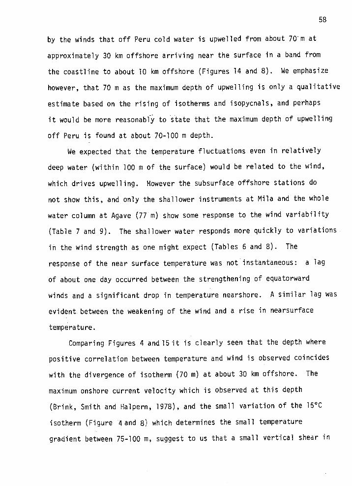
by the winds that off Peru cold water is upwelled from about 70m at
approximately 30 km offshore arriving near the surface in a band from
the coastline to about 10 km offshore (Figures 14 and 8). We emphasize
however, that 70 m as the maximum depth of upwelling is only a qualitative
estimate based on the rising of isotherms and isopycnals, and perhaps
it would be more reasonabi' to state that the maximum depth of upwelling
off Peru is found at about 70-100 m depth.
We expected that the temperature fluctuations even in relatively
deep water (within 100 rn of the surface) would be related to the wind,
which drives upwelling. However the subsurface offshore stations do
not show this, and only the shallower instruments at Mila and the whole
water column at Agave (77 m) show some response to the wind variability
(Table 7 and 9). The shallower water responds more quickly to variations
in the wind strength as one might expect (Tables 6 and 8). The
response of the near surface temperature was not instantaneous: a lag
of about one day occurred between the strengthening of equatorward
winds and a significant drop in temperature nearshore. A similar lag was
evident between the weakening of the wind and a rise in nearsurface
temperature.
Comparing Figures 4 and 15 it is clearly seen that the depth where
positive correlation between temperature and wind is observed coincides
with the divergence of isotherm (70 m) at about 30 km offshore. The
maximum onshore current velocity which is observed at this depth
(Brink, Smith and Halpern, 1978), and the small variation of the 15°C
isotherm (Figure 4and 8) which determines the small temperature
gradient between 75-100 m, suggest to us that a small vertical shear in

59
the alongshore current velocity would also be observed. Changes on the
direction of the current nearshore and at the upper slope should be related
with changes in the thermal structure (VT) suggesting the potential
validity of the thermal wind equation. In order to explore how the
thermal-wind equation holds, spectral analysis with current and
temperature time series wóuld be useful.
Observing the wind records at the different stations (Figure 5)
it is apparent that the fluctuations of the alongshore wind are
correlated significantly over the area of measurements (Tables 2 and
3). Despite this fact the significant departure of the results for
correlation between temperature and wind at PD with that which results
for nearshore winds at PSS and Parodia (Table 9) suggest to us that
perhaps the temperature nearshore responds more to very high
frequency while temperature offshore is better responding to very low
frequency; spectral analysis for wind time series might answer this
question.
Additional research is required before conclusive answers can be
found regarding the relationship between temperature time series,
hydrography and wind, mainly to determine the physical process
involved in maintaining the different regimes observed.
V. REFERENCES
Barton, E. D. 1977. JOINT-lI - R/V THOMAS G. THOMPSON Cruise 108,Leg 1, CTD measurements off the coast of Peru near Cabo Nazca,April-May 1976. International Decade of Ocean Exploration,Coastal Upwelling Ecosystems Analysis. Data Report 39, 140 pp.
Barton, E. D., A. Huyer and R. L. Smith. 1977. Temporal variationobserved in the hydrographic regime near Cabo Corveiro in theNorthwest African upwelling region, February to April 1974,Deep-Sea Res., 24: 7-23.
Bendat, J. S. and A. G. Piersol. 1966. Measurements and analysisof random data. New York, John Wiley and Son. 390 pp.
Brink, K. H., J. S. Allen and R.L. Smith. 1978. A study of lowfrequency fluctuations near the Peru coast, submitted to J.Phys. Oceanogr.
Brink, K. D., D. Halpern and R. L. Smith. 1978. A preliminaryprospectus of a compendium of the time-series measurements frommoored instrumentation during the MAM 77 phase of JOINT-Il. In
preparation.
Crow, E. L., F. A. Davis and 11. W. Maxfield. 1969. Statistics Manual.
New York, Dover Publications. 288 pp.
Davis, R. E. 1976. Predictability of sea surface temperature and sealevel pressure anomalies over the North Pacific Ocean. J. Phys.
Oceanogr., 6: 249-266.
Enfield, D. B. 1970. A mesoscale study of coastal currents andupwelling off Peru. M. S. dissertation, Oregon State University,Corvallis, Oregon. 67 pp.
Enfield, D. B., R. L. Smith and A. Huyer. 1978. A compilation ofobservations from moored current meters. Vol. XII, Winds, currentsand temperature over the continental shelf and slope off Peru duringJOINT-Il, March 1976-May 1977. Oregon State University, School ofOceanography, Corvallis, Oregon. Data Report 70. Reference 78-4.
343 pp.
Halpern, D. 1974. Variation in the density field during coastalupwelling. Tethys, 6(l-2):363-374.
Halpern, D. 1976. Structure of a coastal upwelling event observedoff Oregon during July 1973. Deep-Sea Res., 23:495-508.
61
Halpern, D. 1978. JOINT-2 near-surface circulation studies:Progress Report 1. Coastal Upwellirig Ecosystems Analysis.
Synapse Notes, No. 2, 2-13.
Halpern, D., T. R. Holbrook, and R. M. Reynolds. 1974. A compilationof wind, current and temperature measurements: Oregon, July andAugust 1973. CUEA Tech. Rept. 6, Ref. M74-73, Dept. ofOceanography, University of Washington, 190 pp.
Huyer, A. 1976. A compaison of upwelling events in two locations:Oregon and Northwest Africa. J. Mar. Res., 34:531-546.
Medina, F. A. 1978. A continuous time series of the wind atPta. San Juan, Peru, during JOINT-Il. Coastal Upwelling Eco-systems Analysis. Synapse Notes No. 4, 1-13.
Mittelstaedt, E., R. D. Pillsbury and R. L. Smith. 1975. Flow
patterns in the Northwest African upwelling area. Dr. Hydrogr. Z.
28:145-167.
Ochs, L., J. A. Baughman and J. Ballance. 1973. OS-3 ARAND SYSTEM:Documentation and examples, Vol I. CCR-70-4. O.S.U. ComputerCenter, Oregon State University, Corvallis, Oregon. 155 p.
Pearson, E. S. and H. 0. Hartley, editors. 1970. Brometrika
Tables for Statisticians. Cambridge University Press, 270 pp.
Pillsbury, R. D. 1972. descriDtion of hydrography, winds and currentduring the upwelling season near Newport, Oregon. Ph.D.
Dissertation, Oregon State University, Corvallis, Oregon. 163 pp.
Pillsbury, R. 0., J. S. Bottero, R. E. Still and W. E. Gilbert. 1974.
A compilation of observations from moored current meters,Vol. VI, Oregon continental shelf, April-October 1972. Oregon
State University, School of Oceanography, Corvallis. Data Report
57, Reference 74-2.
Smith, R. L. 1964. An investigation of upweuling along the Oregoncoast. Ph.D. Dissertation. Oregon State University, Corvallis.83 numbered pages.
Smith, R. L. 1968. Upwelling. Oceanogr. Mar. Biol. Ann. Rev., 6:11-46.
Stuart, D. W. 1978. Wind events during JOINT-Il. Coastal Upwelling
Ecosystems Analysis. Synapse Notes No. 2, 13-18.
Wooster, W. S. and M. Gilmartin. 1961. The Peru-Chile undercurrent.
J. Mar. Res., 19:97-122.

Wyrtki, K. 1963. The horizontal and vertical field of motion in thePeru current. Bull. Scripps Inst. Oceanogr., 8:313-346.
Wyrtki, K. 1964. The thermal structure of the Eastern Pacific Ocean.Dt. Hydrogr. Z., Erganzungsh. A., 6, 84 pp.
Zuta, S., T. Rivera and A. Bustamante. 1975. Hydrological aspectsof the main upwelling areas off Peru. Paper presented at theThird International Symposium on Upwelling Ecosystem, Kiel,August 25-28, 1975.