adaptive fusion of multisensor precipitation using …efi.eng.uci.edu/papers/efg_113.pdf · ·...

Adaptive fusion of multisensor precipitation using Gaussian‐scalemixtures in the wavelet domain

Ardeshir Mohammad Ebtehaj1,2 and Efi Foufoula‐Georgiou1

Received 7 May 2011; revised 20 August 2011; accepted 22 August 2011; published 19 November 2011.

[1] The past decades have witnessed a remarkable emergence of new sources ofmultiscale multisensor precipitation data, including global spaceborne active and passivesensors, regional ground‐based weather surveillance radars, and local rain gauges. Optimalintegration of these multisensor data promises a posteriori estimates of precipitation fluxeswith increased accuracy and resolution to be used in hydrologic applications. In thiscontext, a new framework is proposed for multiscale multisensor precipitation data fusionwhich capitalizes on two main observations: (1) non‐Gaussian statistics of precipitationimages, which are concisely parameterized in the wavelet domain via a class ofGaussian‐scale mixtures, and (2) the conditionally Gaussian and weakly correlatedlocal representation of remotely sensed precipitation data in the wavelet domain, whichallows for exploiting the efficient linear estimation methodologies while capturing thenon‐Gaussian data structure of rainfall. The proposed methodology is demonstrated usinga data set of coincidental observations of precipitation reflectivity images by thespaceborne precipitation radar aboard the Tropical Rainfall Measurement Mission satelliteand by ground‐based weather surveillance Doppler radars.

Citation: Ebtehaj, A. M., and E. Foufoula‐Georgiou (2011), Adaptive fusion of multisensor precipitation using Gaussian‐scalemixtures in the wavelet domain, J. Geophys. Res., 116, D22110, doi:10.1029/2011JD016219.

1. Introduction

[2] Availability of multisensor observations and the desirefor accurate high‐resolution forecasts have always been astrong motivation to explore algorithms for optimal inte-gration of multisensor, multiscale geophysical data into amore complete set of information with reduced uncertainty.In the last decade, a large set of multiscale precipitation datahas been collected using locally distributed traditional net-works of rain gauges and regional ground‐based weathersurveillance radars, e.g., Next Generation Radar (NEXRAD)and global spaceborne active and passive satellite sensors,e.g., Tropical Rainfall Measuring Mission (TRMM). Theacquired remotely sensed precipitation data might bemathematically understood as the convolution of the highlyirregular reflectivity field of the atmospheric hydrometeorswith a low‐pass operator, naturally corrupted with noise dueto intrinsic measurement fluctuations or to sensor noise.Several studies have been conducted to characterize themeasurement error of the remotely sensed precipitation data[e.g., Ciach and Krajewski, 1999; Wang and Wolff, 2009],whereas much less attention has been devoted to developingconsistent and robust algorithms that can be used to filter out

these errors and optimally merge (fuse) the multisensor datafor obtaining a posteriori estimates of the precipitationfields.[3] The standard linear Gaussian filtering methods on

Markov treelike structures, the so‐called scale‐recursiveestimation (SRE) technique, has been commonly proposedto assimilate remotely sensed rainfall observations at dif-ferent scales into a stochastic (e.g., multiplicative randomcascade) model of rainfall fields [Gorenburg et al., 2001;Tustison et al., 2002; Gupta et al., 2006; Bocchiola andRosso, 2006; Bocchiola, 2007; Van de Vyver and Roulin,2009]. The main advantage of this method is its efficiencyto provide a recursive least squares solution for high‐dimensional multiscale Gauss‐Markov estimation problems.Consequently, by construction, fusion of multisensor rainfalldata using SRE is based on the assumption that the multi-scale statistical structure of the precipitation fields (or logtransformed fields) is linear and can be explained in theGaussian domain.[4] Early observations signified that spatial rainfall exhi-

bits a clustered behavior [e.g., LeCam, 1961], meaning thatareas of high‐intensity precipitation, referred to as “rainfallcells,” tend to occur in clusters within regions of lower rainrate. This had been the earliest motivation for modelingapproaches that sought to represent the observed geometryand statistical structure of precipitation by means of clus-tered point processes [e.g., see Gupta and Waymire, 1993].These isolated high‐intensity clusters of rainfall cells man-ifest themselves in the tail statistics of the rainfall histogramwhich are remarkably thicker than the domain of Gaussiandistributions, including the lognormal density [Ebtehaj and

1Saint Anthony Falls Laboratory, Department of Civil Engineering andNational Center for Earth‐Surface Dynamics, University of Minnesota,Twin Cities, Minneapolis, Minnesota, USA.

2School of Mathematics, University of Minnesota, Twin Cities,Minneapolis, Minnesota, USA.

Copyright 2011 by the American Geophysical Union.0148‐0227/11/2011JD016219

JOURNAL OF GEOPHYSICAL RESEARCH, VOL. 116, D22110, doi:10.1029/2011JD016219, 2011

D22110 1 of 19

http://dx.doi.org/10.1029/2011JD016219

Foufoula‐Georgiou, 2010, 2011]. These observations indi-cate that by using the SRE method for rainfall multiscaleestimation problems, important high‐order statistical char-acteristics of rainfall cannot be thoroughly captured and theresult of the rainfall data fusion may be an overly smoothrepresentation without adequate detailed features of thestorm rainfall cells and extreme intensity values. This obvi-ously calls for developing consistent and well‐structuredfiltering and fusion methodologies that can efficientlyaddress the distinct non‐Gaussian estimation issues of high‐dimensional precipitation fields and also permit incorpora-tion of different sources of the multiscale measurementerrors in the fusion process.[5] Recent studies [Ebtehaj and Foufoula‐Georgiou, 2011]

demonstrated that a particular mixture of Gaussian randomvariables can well capture the observed heavy tail propertiesof the precipitation data in the wavelet domain. In this paper,we will explain how this probability model in the waveletdomain can be exploited for optimal multiscale fusion ofmultisensor precipitation data. Using the developed meth-odology, we present a case study in which, first, rain gaugecorrected products are derived via filtering the measurementerror from the coincidental observations of the TRMM‐PRsatellite and ground‐based NEXRAD reflectivity data and,second, the rain gauge corrected products are merged in amultiscale framework. The advantages of the introducedmethod over the conventional linear Gaussian estimationtechnique are also discussed. Accordingly, this paper isstructured as follows:[6] Section 2 is devoted to briefly discussing the statistics

and non‐Gaussian structure of rainfall reflectivity imagesin the wavelet and Fourier domains. In the context of pre-cipitation multisensor fusion, the standard linear Gaussianestimation method is explained and implemented in section 3.Practical aspects of implementation and shortcomings of this

method are also discussed in section 3. Section 4 explainsthe new proposed probability model, namely the Gaussian‐scale mixture (GSM), for precipitation reflectivity imagesin the wavelet domain which can be used for consistentand robust multiscale multisensor data fusion. In section 5,basic theoretical and practical concepts of optimal estimationin the wavelet domain using the GSM probability modelare explained. A synthetic one‐dimensional example is alsopresented to elaborate the main advantages of the proposedmethodology compared with the SRE method. Section 6describes the implementation of the new model for pre-cipitation estimation and data fusion by applying it to areal storm event coincidentally measured by ground‐basedNEXRAD and TRMM‐PR sensors. Section 7 presents asummary of the study and points out some directions forfuture research.

2. Non‐Gaussian Statistics of PrecipitationImages

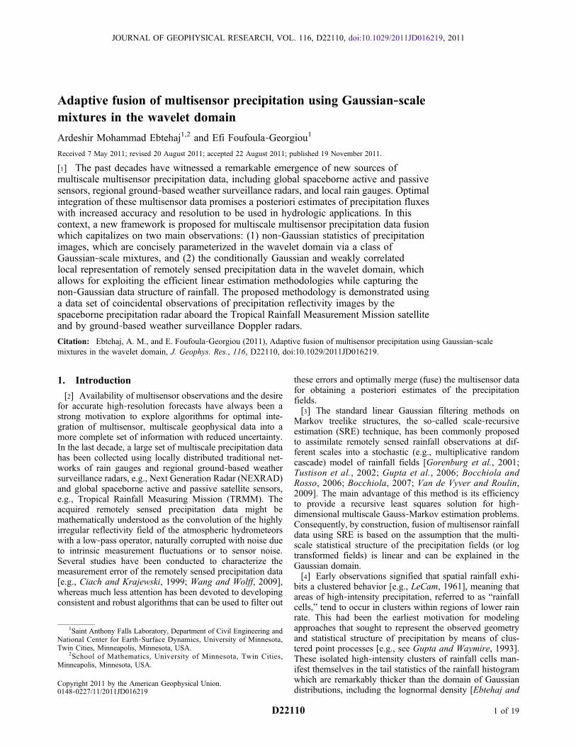
[7] Ebtehaj and Foufoula‐Georgiou [2011] studied thestatistical structure of a data set populated by near‐surfaceprecipitation images in decibels of reflectivity (dBZ), fromtwo hundred independent storms coincidentally observed byNEXRAD and TRMM precipitation radars over two TRMMground validation (GV) sites in Houston, Texas (HSTN) andMelbourne, Florida (MELB). It was demonstrated that theFourier and wavelet decompositions of these fields permitconcise parameterization across a range of spatial scales.Specifically, it was revealed that besides the power lawdecay of the Fourier spectra (see Figure 1a), the distributionof the wavelet coefficients (smoothed increments) shows asymmetric cusp singularity around the center with extendedheavy tails significantly thicker than the Gaussian case (seeFigure 1b). Although the conversion of rainfall reflectivity

Figure 1. (a) Radially averaged ensemble spectrum of 105 NEXRAD precipitation single‐level near‐surface reflectivity images at resolution 1 × 1 km over the ground validation site of the TRMM satellitein Melbourne, Florida. Frequencies are in cycle per pixel (c/p), which are equivalent to the inverse ofpseudo spatial scale km−1. (b) Associated average histogram of the horizontal subband coefficients d.The solid circles show the mean empirical histogram, and the solid line is the fitted generalized Gaussiandistribution p(x) / exp (−∣x=s∣a). The dashed lines are the 95% estimation quantiles.

EBTEHAJ AND FOUFOULA‐GEORGIOU: PRECIPITATION MULTISENSOR FUSION D22110D22110

2 of 19

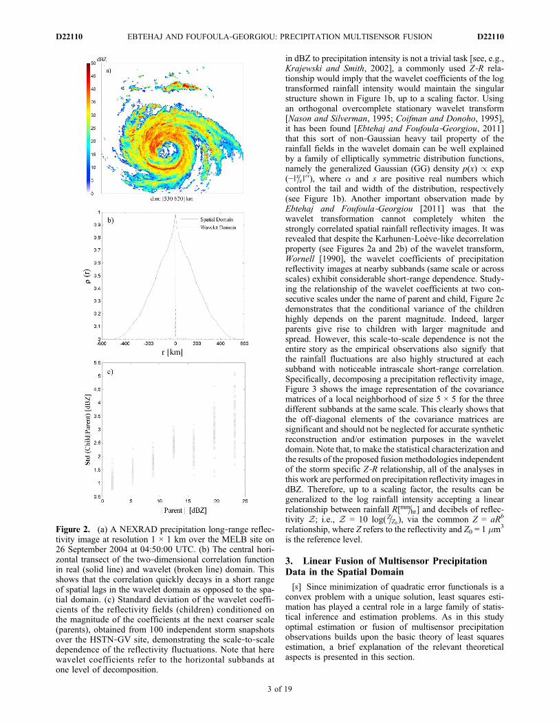
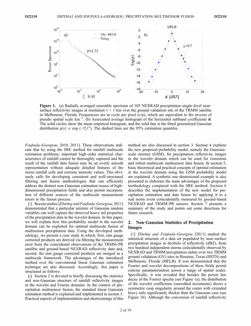
in dBZ to precipitation intensity is not a trivial task [see, e.g.,Krajewski and Smith, 2002], a commonly used Z‐R rela-tionship would imply that the wavelet coefficients of the logtransformed rainfall intensity would maintain the singularstructure shown in Figure 1b, up to a scaling factor. Usingan orthogonal overcomplete stationary wavelet transform[Nason and Silverman, 1995; Coifman and Donoho, 1995],it has been found [Ebtehaj and Foufoula‐Georgiou, 2011]that this sort of non‐Gaussian heavy tail property of therainfall fields in the wavelet domain can be well explainedby a family of elliptically symmetric distribution functions,namely the generalized Gaussian (GG) density p(x) / exp(−∣x=s∣a), where a and s are positive real numbers whichcontrol the tail and width of the distribution, respectively(see Figure 1b). Another important observation made byEbtehaj and Foufoula‐Georgiou [2011] was that thewavelet transformation cannot completely whiten thestrongly correlated spatial rainfall reflectivity images. It wasrevealed that despite the Karhunen‐Loève‐like decorrelationproperty (see Figures 2a and 2b) of the wavelet transform,Wornell [1990], the wavelet coefficients of precipitationreflectivity images at nearby subbands (same scale or acrossscales) exhibit considerable short‐range dependence. Study-ing the relationship of the wavelet coefficients at two con-secutive scales under the name of parent and child, Figure 2cdemonstrates that the conditional variance of the childrenhighly depends on the parent magnitude. Indeed, largerparents give rise to children with larger magnitude andspread. However, this scale‐to‐scale dependence is not theentire story as the empirical observations also signify thatthe rainfall fluctuations are also highly structured at eachsubband with noticeable intrascale short‐range correlation.Specifically, decomposing a precipitation reflectivity image,Figure 3 shows the image representation of the covariancematrices of a local neighborhood of size 5 × 5 for the threedifferent subbands at the same scale. This clearly shows thatthe off‐diagonal elements of the covariance matrices aresignificant and should not be neglected for accurate syntheticreconstruction and/or estimation purposes in the waveletdomain. Note that, to make the statistical characterization andthe results of the proposed fusion methodologies independentof the storm specific Z‐R relationship, all of the analyses inthis work are performed on precipitation reflectivity images indBZ. Therefore, up to a scaling factor, the results can begeneralized to the log rainfall intensity accepting a linearrelationship between rainfall R[mm=hr] and decibels of reflec-tivity Z; i.e., Z = 10 log(Z=Z0 ), via the common Z = aRb

relationship, where Z refers to the reflectivity and Z0 = 1 mm3

is the reference level.

3. Linear Fusion of Multisensor PrecipitationData in the Spatial Domain

[8] Since minimization of quadratic error functionals is aconvex problem with a unique solution, least squares esti-mation has played a central role in a large family of statis-tical inference and estimation problems. As in this studyoptimal estimation or fusion of multisensor precipitationobservations builds upon the basic theory of least squaresestimation, a brief explanation of the relevant theoreticalaspects is presented in this section.

Figure 2. (a) A NEXRAD precipitation long‐range reflec-tivity image at resolution 1 × 1 km over the MELB site on26 September 2004 at 04:50:00 UTC. (b) The central hori-zontal transect of the two‐dimensional correlation functionin real (solid line) and wavelet (broken line) domain. Thisshows that the correlation quickly decays in a short rangeof spatial lags in the wavelet domain as opposed to the spa-tial domain. (c) Standard deviation of the wavelet coeffi-cients of the reflectivity fields (children) conditioned onthe magnitude of the coefficients at the next coarser scale(parents), obtained from 100 independent storm snapshotsover the HSTN‐GV site, demonstrating the scale‐to‐scaledependence of the reflectivity fluctuations. Note that herewavelet coefficients refer to the horizontal subbands atone level of decomposition.


3 of 19

3.1. Principles of Least Squares Estimation

[9] Consider a set of noisy measurements y 2 RN of aparameter vector x 2 RK with joint covariance matrix of theform S = [Sx, Sxy; Syx, Sy]. Without having any a prioriassumption about the density of observations and parametervectors, the Bayesian least squares estimator of x and theassociated covariance (S) of estimation can be derived as,

x ¼ mx þ SxyS�1y y� my

� �Sx ¼ Sx � SxyS�1

y Syx;

where mx = E[x] and my = E[y] [see, e.g., Levy, 2008].[10] Casting this problem in the context of a linear mea-

surement equation of the form y = Cx + v in the Gaussiannoise environment v ∼ N (0, Sv), where C 2 RN×K is themeasurement matrix, and knowing SAx, By = ASxyB

T for any

matrices A and B of relevant size, the above expression canbe further expanded as follows.

x ¼ mx þ SxCT CSxC

T þ Sv

� ��1y� Cmxð Þ ð1Þ

Sx ¼ Sx � SxCT CSxC

T þ Sv

� ��1CSx: ð2Þ

[11] The least squares estimation x of x given y, is indeedthe projection of x onto the linear subspace spanned by y orsay span{y}, which is optimal in the sense that E [∣x − x∣2] ≤E [∣x − span{y}∣2]. In the case that x and y are in the Gaussiandomain (linear filtering), the least squares estimator is fullyoptimal in the sense that it coincides with the conditionalexpectation x = E [x∣y]. However, in the case of non‐Gaussian distributions (nonlinear filtering), the conditionalexpectation is a nonlinear function of the measurements and

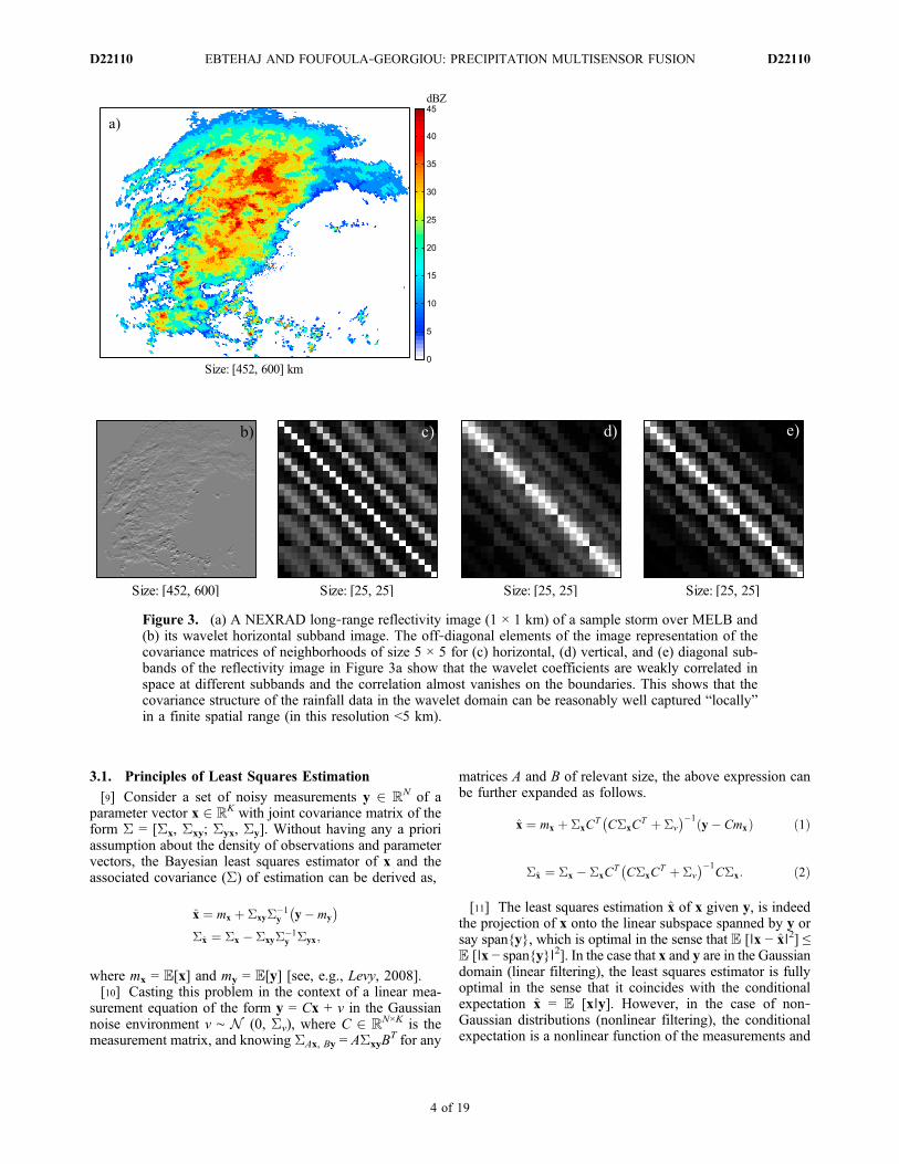
Figure 3. (a) A NEXRAD long‐range reflectivity image (1 × 1 km) of a sample storm over MELB and(b) its wavelet horizontal subband image. The off‐diagonal elements of the image representation of thecovariance matrices of neighborhoods of size 5 × 5 for (c) horizontal, (d) vertical, and (e) diagonal sub-bands of the reflectivity image in Figure 3a show that the wavelet coefficients are weakly correlated inspace at different subbands and the correlation almost vanishes on the boundaries. This shows that thecovariance structure of the rainfall data in the wavelet domain can be reasonably well captured “locally”in a finite spatial range (in this resolution <5 km).


4 of 19

the least squares estimator is just a suboptimal linear esti-mation of the conditional expectation. Note that in general,the conditional expectation is optimal in the sense thatE [∣x − E [x∣y]∣2] ≤ E [∣x − f (y)∣2], where f (y) denotes anynonlinear function of the observations [see Fristedt et al.,2007; Levy, 2008]. In practice, for high‐dimensional pro-blems obtaining this estimator may require inversion of themeasurement covariance matrix, which might be compu-tationally cumbersome especially in temporal systems whileonline measurements become available sequentially andcumulative in time.[12] A least squares estimation paradigm was introduced

by Kalman [1960] for the estimation of discrete time linearGauss‐Markov stochastic processes, i.e., xt = At−1xt−1 + wt−1,where At is the temporal transition matrix and wt ∼N (0, Swt

)is a white Gaussian noise vector, known as the model error.Minimizing the trace of the covariance matrix of the esti-mates, this formalism allows us to sequentially obtain theconditional expectation of the system state variables xt =E [xt∣y0,y1,…,yt] in time, given the noisy observations in theframework of an affine measurement equation yt = Ctxt + vt,where Ct relates the system state to the measurements andvt ∼ N (0, Svt). Obviously, for such a Gaussian dynamicsystem, Kalman filter (KF) is an optimal estimator as theconditional expectation, and the associated covariance canfully explain the entire probabilistic structure of the sys-tem. Replacing the notion of time with scale, the originalidea of the linear estimation of temporal Gauss‐Markovsystems was further expanded by Chou et al. [1994] to theoptimal estimation of multiresolution auto‐regressive (MAR)Gaussian processes [e.g., Luettgen et al., 1993; Daniel andWillsky, 1999; Willsky, 2002]. In MAR representation, amultiresolution process is naturally defined on a treelikegraph structure T (see Figure 4), where each node s 2 T on

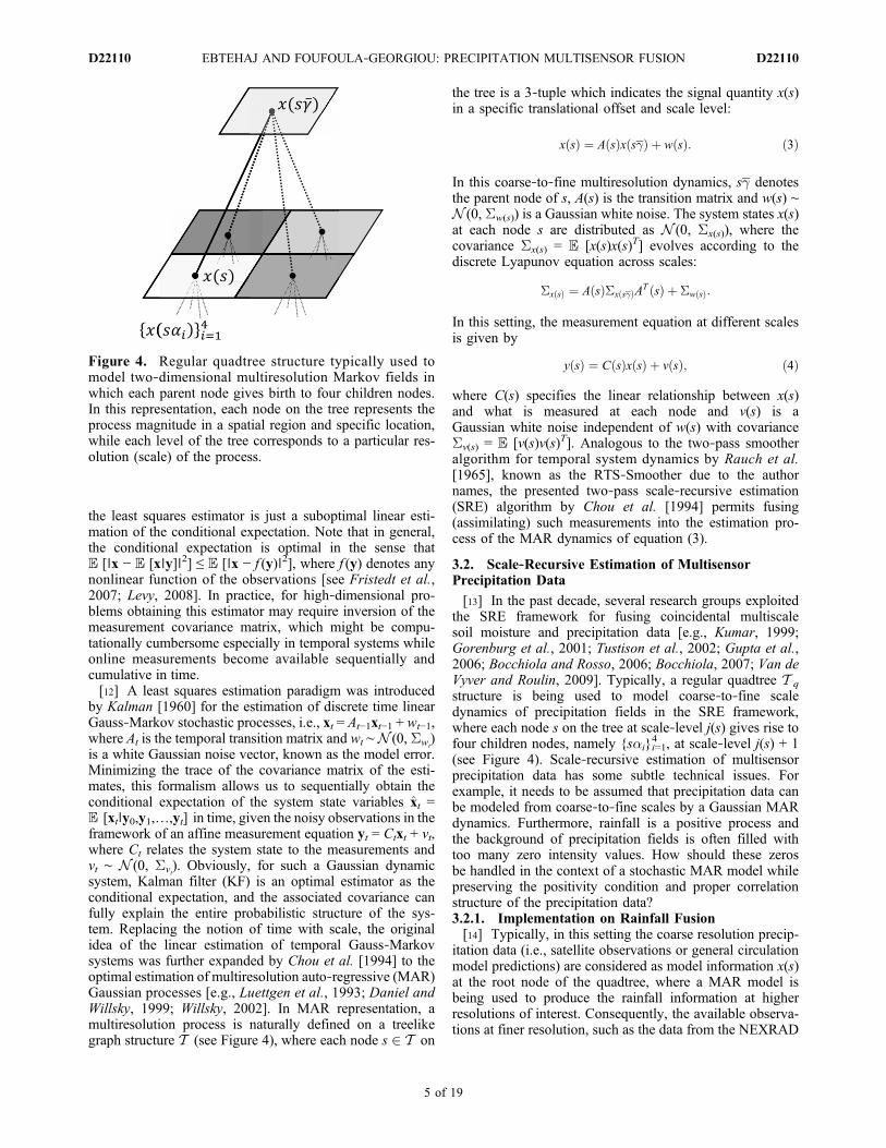
the tree is a 3‐tuple which indicates the signal quantity x(s)in a specific translational offset and scale level:

x sð Þ ¼ A sð Þx s�ð Þ þ w sð Þ: ð3Þ

In this coarse‐to‐fine multiresolution dynamics, s� denotesthe parent node of s, A(s) is the transition matrix and w(s) ∼N (0, Sw(s)) is a Gaussian white noise. The system states x(s)at each node s are distributed as N (0, Sx(s)), where thecovariance Sx(s) = E [x(s)x(s)T] evolves according to thediscrete Lyapunov equation across scales:

Sx sð Þ ¼ A sð ÞSx s�ð ÞAT sð Þ þ Sw sð Þ:

In this setting, the measurement equation at different scalesis given by

y sð Þ ¼ C sð Þx sð Þ þ v sð Þ; ð4Þ

where C(s) specifies the linear relationship between x(s)and what is measured at each node and v(s) is aGaussian white noise independent of w(s) with covarianceSv(s) = E [v(s)v(s)T]. Analogous to the two‐pass smootheralgorithm for temporal system dynamics by Rauch et al.[1965], known as the RTS‐Smoother due to the authornames, the presented two‐pass scale‐recursive estimation(SRE) algorithm by Chou et al. [1994] permits fusing(assimilating) such measurements into the estimation pro-cess of the MAR dynamics of equation (3).

3.2. Scale‐Recursive Estimation of MultisensorPrecipitation Data

[13] In the past decade, several research groups exploitedthe SRE framework for fusing coincidental multiscalesoil moisture and precipitation data [e.g., Kumar, 1999;Gorenburg et al., 2001; Tustison et al., 2002; Gupta et al.,2006; Bocchiola and Rosso, 2006; Bocchiola, 2007; Van deVyver and Roulin, 2009]. Typically, a regular quadtree T q

structure is being used to model coarse‐to‐fine scaledynamics of precipitation fields in the SRE framework,where each node s on the tree at scale‐level j(s) gives rise tofour children nodes, namely {sai}i=1

4 , at scale‐level j(s) + 1(see Figure 4). Scale‐recursive estimation of multisensorprecipitation data has some subtle technical issues. Forexample, it needs to be assumed that precipitation data canbe modeled from coarse‐to‐fine scales by a Gaussian MARdynamics. Furthermore, rainfall is a positive process andthe background of precipitation fields is often filled withtoo many zero intensity values. How should these zerosbe handled in the context of a stochastic MAR model whilepreserving the positivity condition and proper correlationstructure of the precipitation data?3.2.1. Implementation on Rainfall Fusion[14] Typically, in this setting the coarse resolution precip-

itation data (i.e., satellite observations or general circulationmodel predictions) are considered as model information x(s)at the root node of the quadtree, where a MAR model isbeing used to produce the rainfall information at higherresolutions of interest. Consequently, the available observa-tions at finer resolution, such as the data from the NEXRAD

Figure 4. Regular quadtree structure typically used tomodel two‐dimensional multiresolution Markov fields inwhich each parent node gives birth to four children nodes.In this representation, each node on the tree represents theprocess magnitude in a spatial region and specific location,while each level of the tree corresponds to a particular res-olution (scale) of the process.


5 of 19

weather surveillance radars, are generally considered asmeasurements y(s).[15] In the context of rainfall data, it has long been argued

[e.g., Lovejoy and Schertzer, 1990; Gupta and Waymire,1993] that these fields can be explained using a nonlinearmultiplicative scale‐to‐scale stochastic structure; e.g., r(s) =r(s�)z(s), where z(s) represents a driving random compo-nent known as the cascade generator with E [z(s)] = 1, ina canonical form. Working on high‐resolution rainfall data,Menabde et al. [1997] proposed a lognormal density for thez(s). To treat this nonlinear recursion and make it consistentwith the settings in equations (3) and (4), typically the SREmethod is performed in the log transformed rainfall; i.e., log[r(s)]: = x(s), or say a shifted version of the reflectivityfields [e.g., Gorenburg et al., 2001; Tustison et al., 2002],

log r sð Þ½ � ¼ log r s�ð Þ½ � þ log � sð Þ½ �; ð5Þ

where log[z(s)] is a Gaussian white noise, equivalent to theterm w(s) in equation (3). In terms of the first‐order andmarginal statistics, this transformation seems fine; however,the log transformation cannot completely transform a rain-fall field into a Gaussian process and change the multipli-cative scale‐to‐scale correlation into an additive structure.For instance, it is easy to check that the conditional variancein a multiplicative recursion depends on the magnitude ofthe process at the next coarser scale; i.e., var [r(s)∣r(s�)] =(r(s�))2 var [z(s)], which is not the case in equation (5), aslong as the term log[z(s)] remains a “white” type of Gaussiannoise at different scales. In effect, some important higher‐order scale‐to‐scale statistical structures are ignored in linearestimation of rainfall data in the log transformed domain.Moreover, we have also shown that the marginal histogramof the rainfall reflectivity data (logarithm of rainfall throughZ‐R relationship) is far from being in the Gaussian domain ofattraction (see Figure 1b) [Ebtehaj and Foufoula‐Georgiou,2010, 2011].[16] Considering all of these major MAR model incom-

patibilities with the observed statistical structure of rainfall,the standard Gaussian multiscale filtering technique stillprovides a very efficient global least square estimator ofthe multiscale multisensor precipitation data. Here an exam-ple is provided which uses the SRE framework to mergeprecipitation given from TRMM‐PR and ground‐basedNEXRAD coincidental precipitation reflectivity imageries.We assumed that the reflectivity images can be partiallyexplained by the linear MAR model in equation (3). The treeis assumed stationary in the sense that A(s) = I and asexplained the “model” information x(s) is obtained from thecoarse resolution TRMM near‐surface reflectivity images at≈4 × 4 km and the “observations” y(s) are set to theNEXRAD high‐resolution reflectivity imageries at 1 × 1 km.We assumed that both sensors provide unbiased precipita-tion estimates in a global sense and hence we set C(s) = I. Toaddress the self‐similarity and commonly observed 1/f spec-trum in the rainfall reflectivity images (see, e.g., Figure 1a),it is assumed that the variance of the driving noise term w(s)decays geometrically from coarse‐to‐fine scales by assigningSw(s) / 2−Hj(s)I, where the scalar parameter H > 0 refersto the self‐similarity index, and j(s) represents coarse‐to‐finescale levels at node s. This parameter controls the dropoff

rate of the power spectrum of the synthesized fields [Danieland Willsky, 1999] and can be estimated from the availablehigh‐resolution NEXRAD data. To this end, we simplyemployed the concept of image pyramid encoding [Burt andAdelson, 1983]. The original NEXRAD image can becoarsened by smoothing and downsampling by a factorof 2, using an average filter of size 2 × 2, to produce an“approximate” representation of the field at the next coarserscale. The approximate coarse scale image is then upsampledby a factor of 2 and convolved with a nearest neighborhoodinterpolator to produce the so‐called “prediction field,”whichwill have the same dimensions as the original NEXRADimage. The difference between the prediction field and theoriginal one indeed gives us the “detail information” whichis needed to reconstruct perfectly the high‐resolution origi-nal image given the low‐resolution (approximate) versionat the next coarser scale [see Gonzalez and Woods, 2008].Recursive implementation of this encoding procedure yieldscharacterization of the scale‐to‐scale detail information andcharacterization of the noise term w(s) in equation (3).Indeed, we used the high‐resolution NEXRAD precipitationdata to estimate the required self‐similarity exponent of theMAR model to provide TRMM rainfall information x(s) athigher resolution of interest on the tree.[17] The background effect in rainfall fields is significant,

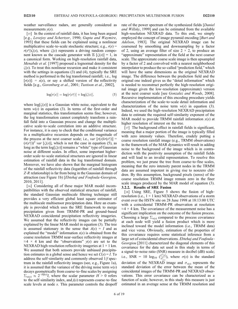
meaning that a major portion of the image is typically filledwith zero intensity values. Therefore, crudely putting acoarse resolution rainfall image (e.g., TRMM observations)in the framework of the MAR dynamics will result in addingnoise to the background of the image which is in contra-diction with the positivity assumption of the rainfall fieldsand will lead to an invalid representation. To resolve thisproblem, we just prune the tree from coarse‐to‐fine scales,meaning that the zero intensity parent nodes in the TRMMdata are assumed impotent in giving rise to nonzero chil-dren. By this assumption, background pixels (zeros) of thecoarse resolution TRMM image remain zero in the finerscale images produced by the MAR model of equation (3).3.2.2. Results of SRE Fusion[18] Using SRE, Figure 5 shows the fusion of high‐

resolution (i.e., 1 × 1 km) NEXRAD observations of a stormevent over the HSTN site on 28 June 1998 at 18:13:00 UTCwith a coincidental TRMM‐PR observation at resolution≈4 × 4 km. The covariance of the measurement noise has asignificant implication on the outcome of the fusion process.Choosing a large Sv(s) compared to the process covarianceat each node will yield a fusion product which is moreinclined toward the model information (i.e., TRMM data)and vice versa. Obviously, estimation of the properties ofthis covariance requires some statistical inference from alarge set of coincidental observations. Ebtehaj and Foufoula‐Georgiou [2011] characterized the diagonal elements of thiscovariance for the data set used in this study in terms ofa signal‐to‐noise ratio (SNR) measure in decibel (dB) scale;i.e., SNR = 10 log10 (�

2 sð Þ�2v sð Þ), where s(s) is the standard

deviation of the NEXRAD image and sv(s) represents thestandard deviation of the error between the mean of thecoincidental images of the TRMM‐PR and NEXRAD obser-vations. This error covariance can be characterized as afunction of scale; however, in this study this measure is justestimated in an average sense at the TRMM resolution and


6 of 19

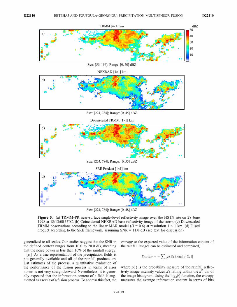
generalized to all scales. Our studies suggest that the SNR inthe defined context ranges from 10.0 to 20.0 dB, meaningthat the noise power is less then 10% of the rainfall energy.[19] As a true representation of the precipitation fields is

not generally available and all of the rainfall products arejust estimates of the process, a quantitative evaluation ofthe performance of the fusion process in terms of errornorms is not very straightforward. Nevertheless, it is gener-ally expected that the information content of a field is aug-mented as a result of a fusion process. To address this fact, the

entropy or the expected value of the information content ofthe rainfall images can be estimated and compared,

Entropy ¼ �X

kp Zkð Þ log2 p Zkð Þ½ �

where p(·) is the probability measure of the rainfall reflec-tivity image intensity values Zk falling within the kth bin ofthe image histogram. Using the log2(·) function, the entropymeasures the average information content in terms of bits

Figure 5. (a) TRMM‐PR near‐surface single‐level reflectivity image over the HSTN site on 28 June1998 at 18:13:00 UTC. (b) Coincidental NEXRAD base reflectivity image of the storm. (c) DownscaledTRMM observations according to the linear MAR model (H = 0.6) at resolution 1 × 1 km. (d) Fusedproduct according to the SRE framework, assuming SNR = 11.0 dB (see text for discussion).


7 of 19

per pixel [see Gonzalez and Woods, 2008]. In the studiedstorm images of Figure 5, using SNR = 11.0 dB, as theconsequence of fusion, the average information content of thefinal high‐resolution fused product was increased approxi-mately by 33% compared to the original NEXRAD image.Apart from different probable sources of false detection (e.g.,ground clutter) which need to be treated separately, due tothe inherent differences in the way that the two sensorsinterrogate the vertical profile of the atmosphere, in fusionof precipitation snapshots there might be some spots that asensor detects as rainy areas where the other sensor is blind.Therefore, naturally the wetted area (positive part) of thefused products is greater or equal compared to the individualoriginal measurements. Consequently, a major part of thisentropy increase can be due to the growth of the wetted areaas a natural result of the fusion process.[20] We can also compare matrix norms of the processed

(fused) and unprocessed images (original) to quantify howthis fusion process may affect the overall second‐ordermarginal statistics of the fields. As a result of the fusionprocess, we do expect that the final processed image pos-sesses a 2‐norm measure which falls within the range of the2‐norm of the original input images; i.e., TRMM‐PR andNEXRAD data. To this end, the Frobenius norm (F‐norm) ofthe processed and unprocessed reflectivity images Z 2 RM×N

at two scales of interest are computed and compared:

Zk kF¼

ffiffiffiffiffiffiffiffiffiffiffiffiffiffiffiffiffiffiffiffiffiffiffiffiffiffiffiXMi¼1

XNj¼1

zi; j�� 2

vuut ¼ffiffiffiffiffiffiffiffiffiffiffiffiffiffiffiffiffiffiffitr ZTZ� �

:q

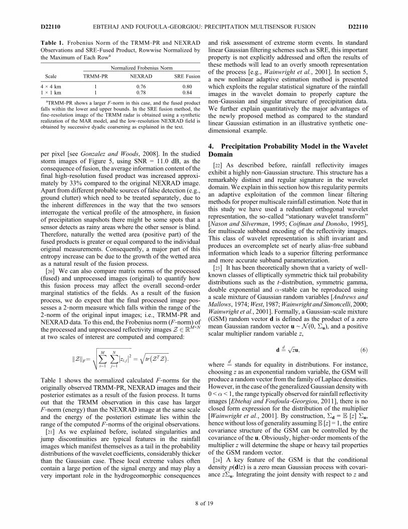
Table 1 shows the normalized calculated F‐norms for theoriginally observed TRMM‐PR, NEXRAD images and theirposterior estimates as a result of the fusion process. It turnsout that the TRMM observation in this case has largerF‐norm (energy) than the NEXRAD image at the same scaleand the energy of the posteriori estimate lies within therange of the computed F‐norms of the original observations.[21] As we explained before, isolated singularities and

jump discontinuities are typical features in the rainfallimages which manifest themselves as a tail in the probabilitydistributions of the wavelet coefficients, considerably thickerthan the Gaussian case. These local extreme values oftencontain a large portion of the signal energy and may play avery important role in the hydrogeomorphic consequences

and risk assessment of extreme storm events. In standardlinear Gaussian filtering schemes such as SRE, this importantproperty is not explicitly addressed and often the results ofthese methods will lead to an overly smooth representationof the process [e.g., Wainwright et al., 2001]. In section 5,a new nonlinear adaptive estimation method is presentedwhich exploits the regular statistical signature of the rainfallimages in the wavelet domain to properly capture thenon‐Gaussian and singular structure of precipitation data.We further explain quantitatively the major advantages ofthe newly proposed method as compared to the standardlinear Gaussian estimation in an illustrative synthetic one‐dimensional example.

4. Precipitation Probability Model in the WaveletDomain

[22] As described before, rainfall reflectivity imagesexhibit a highly non‐Gaussian structure. This structure has aremarkably distinct and regular signature in the waveletdomain.We explain in this section how this regularity permitsan adaptive exploitation of the common linear filteringmethods for proper multiscale rainfall estimation. Note that inthis study we have used a redundant orthogonal waveletrepresentation, the so‐called “stationary wavelet transform”[Nason and Silverman, 1995; Coifman and Donoho, 1995],for multiscale subband encoding of the reflectivity images.This class of wavelet representation is shift invariant andproduces an overcomplete set of nearly alias‐free subbandinformation which leads to a superior filtering performanceand more accurate subband parameterization.[23] It has been theoretically shown that a variety of well‐

known classes of elliptically symmetric thick tail probabilitydistributions such as the t‐distribution, symmetric gamma,double exponential and a‐stable can be reproduced usinga scale mixture of Gaussian random variables [Andrews andMallows, 1974;West, 1987;Wainwright and Simoncelli, 2000;Wainwright et al., 2001]. Formally, a Gaussian‐scale mixture(GSM) random vector d is defined as the product of a zeromean Gaussian random vector u ∼ N (0, Su), and a positivescalar multiplier random variable z,

d ¼dffiffiz

pu; ð6Þ

where ¼d stands for equality in distributions. For instance,choosing z as an exponential random variable, the GSM willproduce a randomvector from the family of Laplace densities.However, in the case of the generalized Gaussian density with0 < a < 1, the range typically observed for rainfall reflectivityimages [Ebtehaj and Foufoula‐Georgiou, 2011], there is noclosed form expression for the distribution of the multiplier[Wainwright et al., 2001]. By construction, Sd = E [z] Su,hence without loss of generality assumingE [z] = 1, the entirecovariance structure of the GSM can be controlled by thecovariance of the u. Obviously, higher‐order moments of themultiplier z will determine the shape or heavy tail propertiesof the GSM random vector.[24] A key feature of the GSM is that the conditional

density p(d∣z) is a zero mean Gaussian process with covari-ance zSu. Integrating the joint density with respect to z and

Table 1. Frobenius Norm of the TRMM‐PR and NEXRADObservations and SRE‐Fused Product, Rowwise Normalized bythe Maximum of Each Rowa

Scale

Normalized Frobenius Norm

TRMM‐PR NEXRAD SRE Fusion

4 × 4 km 1 0.76 0.801 × 1 km 1 0.78 0.84

aTRMM‐PR shows a larger F‐norm in this case, and the fused productfalls within the lower and upper bounds. In the SRE fusion method, thefine‐resolution image of the TRMM radar is obtained using a syntheticrealization of the MAR model, and the low‐resolution NEXRAD field isobtained by successive dyadic coarsening as explained in the text.


8 of 19

using Bayes’ theorem, the GSM multivariate density can becharacterized as [Wainwright et al., 2001]:

pD dð Þ ¼Z ∞

0p djzð ÞpZ zð Þdz ¼

Z ∞

0

exp � dT zSuð Þ�1d2

� �2�ð ÞN=2 det zSuj jð Þ1=2

p zð Þdz:

[25] A finite dimensional version of this representation isreminiscent of the Gaussian kernel density estimation par-adigm in the statistical literature. Indeed in discrete space,the probability mass function of the GSM is a convexweighted sum of different rescaled versions of some zeromean Gaussian kernels, where given a set of observations,the weights and bandwidths (i.e., pZ(z) and z) of the kernelsneed to be estimated in an optimal sense.

5. GSM Optimal Estimation in the WaveletDomain

5.1. Basics of the Framework

[26] Given a set of independent observations y 2 RN of aGSM random vector d 2 RN (d =

ffiffiz

pu) in a Gaussian noise:

y ¼ dþ v; ð7Þ

where v ∼ N (0, Sv) and assuming E [z] = 1, without loss ofgenerality, equations (6) and (7) result in:

Syjz ¼ zSu þ Sv

Sy ¼ Su þ Sv:ð8Þ

In this case, the likelihood function of the multivariate GSMdensity can be expressed as follows:

p yjzð Þ ¼ 1

2�ð ÞN=2 det zSu þ Svj jð Þ1=2exp

�yT zSu þ Svð Þ�1y2

!:

[27] With no a priori assumption on pZ(z) and perfectwhitening effect of the wavelet transform, Strela [2000] andStrela et al. [2000] derived the maximum likelihood (ML)estimator for the multiplier z. However, as explained previ-ously, it has been found that the wavelet decompositioncannot completely decorrelate the rainfall reflectivity imagesand the wavelet coefficients are highly structured with a shortrange of spatial dependence (see Figures 2a, 2b, and 3). Thisimplies that the assumption about the diagonality of thecovariance matrix of the wavelet coefficients might not be agood assumption for modeling of spatial rainfall.[28] Studying the heavy tail properties of these images

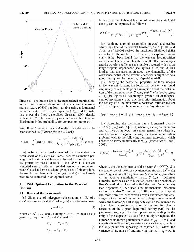
in the wavelet domain, the lognormal density was foundempirically as a suitable prior assumption about the distribu-tion of the multiplier pZ(z) [Ebtehaj and Foufoula‐Georgiou,2011] (see Figure 6). Accordingly, given a set of indepen-dent observations y 2 RN and the a priori information aboutthe density of z, the maximum a posteriori estimate (MAP)of the multiplier can be computed in a Bayesian setting:

zMAP ¼ argmaxz

log p zjyð Þf g ¼ argmaxz

log p yjzð Þ þ log p zð Þ:f g

[29] Assuming the multiplier has a lognormal densityz ∼ LN (mz, sz) with E [z] = 1, where mz and sz are the meanand variance of the log(z), in a more general case where Su

and Sv are not diagonal, solving the above optimizationproblem leads to the following nonlinear expression whichneeds to be solved numerically for zMAP [Portilla et al., 2001,2003],

f zMAPð Þ ¼ log zMAP þ 3�2z=2

zMAP�2z

þ 1

2SN

n¼1

zMAP � ��1n v2n � 1� �

zMAP þ ��1n

� �2 ¼ 0;

ð9Þ

where vn are the components of the vector V = QTS−1y; S isthe square root of the error covariance matrix (i.e., SST = Sv)and (L, Q) contains the eigenvalues ln 2 L and eigenvectorsof the positive semidefinite matrix S−1SuS

−T. Differentnumerical methods such as bisection, secant, false position orBrent’s method can be used to find the root of equation (9)(see Appendix A). We used a multidimensional bisectionmethod [see also Portilla et al., 2001], one of the simplestand most primitive ones which always guarantees the con-vergence to a root as long as the search begins in an intervalwhere the function f (·) takes opposite sign on the boundaries.[30] Note that solving equation (9) requires full charac-

terization of the a priori lognormal density pZ(z) and itsparameters (mz, sz). The assumption corresponding to theunity of the expected value of the multiplier reduces thenumber of unknown parameters to one, as mz +

�2z2 = 0, and

therefore it suffices only to estimate the variance sz2 as it is

the only parameter appearing in equation (9). Given thevariance of the noise sv

2 and knowing that su2 = sy

2 − sv2, it

Figure 6. The broken line is the standardized marginal his-togram (unit standard deviation) of a generated Gaussian‐scale mixture (GSM) random variable using a lognormalmultiplier with sz ≊ 1.2 (see equation (12)), and the solidline shows the fitted generalized Gaussian (GG) densitywith a ≊ 0.7. The inverted parabola shows the Gaussiandistribution in log probability for comparison purposes.


9 of 19

can be shown after some algebra that this parameter can beestimated as (see Appendix A):

�2z ¼ log E z2

� � �¼ log

E y4½ �=3� 2�2y�

2v þ �4

v

�2y � �2

v

� �20B@

1CA: ð10Þ

[31] Assuming that the wavelet coefficients of rainfallimages d 2 RN can be explained using a GSM model with alog prior density for the multiplier, filtering and optimalfusion of different sources of noisy measurements can beperformed efficiently in the wavelet domain while charac-teristic heavy tail distributions and local singularities can bewell captured.[32] In the form of a general linear measurement equation

y = Cd + v, referring to the conditional Gaussian density ofthe GSM model and expressions in equations (1) and (2), theconditional expectation of the zero mean noisy waveletcoefficients and its covariance can be written as:

d ¼ E djy; z½ � ¼ zSuCT C zSuð ÞCT þ Sv½ ��1y

Sd ¼ zSu � z2SuCT C zSuð ÞCT þ Sv½ ��1CSu:

[33] Assuming an unbiased system of measurement equa-tions with identity measurement matrix C = I, given theMAP estimator of the multiplier, this conditional expecta-tion can be simplified into:

E djy; zMAP½ � ¼ zMAPSu zMAPSu þ Svð Þ�1y: ð11Þ

[34] When applied to a local neighborhood of coefficients,this expression is indeed an adaptive local Wiener filterwhich in an individual subband (i.e., a particular scale of

interest) can be exploited to recover the “contaminated”wavelet coefficients in a Gaussian noise environment. Notethat in this setting as the entire structure of the covariancematrix is incorporated, a correlated noise also can be usedand there is no restriction on choosing only a white typeof Gaussian noise (diagonal Sv). Obviously, obtaining thefiltered wavelet coefficients for each subband, a denoisedversion of the process of interest (e.g., rainfall reflectivity)can be recovered using the inverse wavelet transform, whichis optimal both in the least squares and maximum likelihoodsense in the wavelet domain.

5.2. Global Versus Local Filtering

[35] Implementation of the filter discussed above in thewavelet domain requires estimation of Su for each subband,which can be obtained from equation (8) given the mea-surement error covariance Sv. As the wavelet decompositionapproximately whitens the precipitation fields, assuminga finite correlation length for the wavelet coefficients, thiscovariance can be estimated via characterization of thedependence of a local “neighborhood” of the wavelet coef-ficients. In high‐dimensional problems, this local character-ization not only makes the estimation process computationallymore tractable but also leads to a superior estimation, in thesense that the local singular structures of interest (precipita-tion local extremes) can be better recovered from noisyobservations [Strela, 2000; Portilla et al., 2001]. In effect,modulating the measurement covariance by the estimatedmultiplier, the significance of filtering is adaptively adjustedaccording to the local singular features of the field. For largemultiplier values over the singular points of the process, thefiltering is less significant and the filter accepts the obser-vations close to the true values; however, when the multi-plier modulates the Su in the same order of magnitude asthat of the noise covariance, the filter smooths out theobservations by suppressing the noise.[36] In general, a local neighborhood may include clusters

of nearby wavelet coefficients from different subbands atmultiple scales around a reference point. In this study, weuse a pyramidal neighborhood of the wavelet coefficientswhich includes two clusters of the coefficients, each in anindividual subband at two successive scales (see Figure 7).In this construction, the elements of a neighborhood of sizeffiffiffiffiN

p×

ffiffiffiffiN

pof the wavelet coefficients have to be stacked

according to a fixed order into a vector form y 2 RN. Slidingthe neighborhood over the entire subband of size RM×L in anoverlapping manner, the sample covariance matrixSu 2RN×N

can be estimated for each individual subband of largedimension as:

Su �

XM�L

i¼1

yyT� �

i

M � L� Sv:

[37] To resolve the block filtering boundary issues, eachsubband has been padded symmetrically with “mirrorreflection” of itself around the boundaries. For implementa-tion of the GSM‐Wiener filter in equation (11), this covari-ance (Su) only needs to be estimated once for each subband.On the other hand, the multiplier has to be estimated locallyaccording to equation (9) for every neighborhood loca-tion, while it slides over the entire subband domain. The

Figure 7. A general pyramidal neighborhood of size N = 10for each individual wavelet subband where a cluster of3 × 3 pixels (children) is connected to one pixel at the nextcoarser scale (parent). In this multiscale representation of ageneralized neighborhood, scale‐to‐scale and short‐rangeintrascale dependence of the wavelet coefficients can beexplicitly captured in the local covariance matrix. The parentnode information is only taken into account where coarser‐scale subband data are available in the wavelet domain. Inother words, for coarsest‐scale subband information, struc-ture of the generalized neighborhood reduces to a simpleneighborhood of 3 × 3 pixels.


10 of 19

conditional expectation in equation (11) gives an estimateof the entire neighborhood elements, where only the centralvalue needs to be kept as the posterior estimate for eachpoint. This posteriori estimate of the central value is indeeda weighted average of all surrounding elements in the neigh-borhood while the weights are adaptively modulated by theestimated multiplier zMAP.[38] Note that by construction the estimated Su is always

symmetric; however, it may not be positive semidefinite forhigh levels of noise. To ensure the positive semidefinitenessof Su, we first factorized the matrix using eigenvaluedecomposition Su = VDVT and then only nonnegativeeigenvalues {di}i=1

n were picked to reconstruct a positivesemidefinite version of the estimated covariance matrix. Ofcourse, if the leading eigenvalue becomes negative thesubband information cannot be recovered at the assumedpower of noise.

5.3. Synthetic One‐Dimensional Implementation

[39] As previously demonstrated, one of the mainadvantages of the local GSM‐Wiener filter is its adaptabilityto the local structure of the signal compared to its globalstandard Gaussian counterpart (i.e., SRE), leading thus to asuperior estimation of non‐Gaussian heavy tail precipitationfields with frequent isolated intense rainfall clusters. Thispotential achievement and verification may not be very clearwhile filtering out the measurement noise and fusing pre-cipitation images especially when the true intensity valuesof the processes are not available. In this section, a syntheticstudy is conducted to show how this filter provides asuperior framework to recover the true process from noisyobservations of a one‐dimensional multiscale process withnon‐Gaussian heavy tail marginals. For this purpose, anal-ogous to the observed heavy tail multiscale structure of therainfall fluctuations [Ebtehaj and Foufoula‐Georgiou,2011], a one‐dimensional GSM process using a lognormalmultiplier is simulated over a dyadic Markov tree. First, amultiscale nonstationary Gaussian process u(s) is producedon a dyadic tree according to the coarse‐to‐fine scaledynamics of equation (3). The variance of the driving noiseis tuned with a relevant geometrical decay rate from coarse‐to‐fine scales to reproduce an asymptotically dyadic self‐similar process with 1/f spectrum. This process is multipliedelementwise by a sequence of random variables drawn froma lognormal density at different levels of the tree to producea multiscale GSM process on a treelike structure,

u sð Þ ¼ A sð Þu s�ð Þ þ B sð Þw sð Þ

d sð Þ ¼ffiffiffiffiffiffiffiffiz sð Þ

pu sð Þ;

where w(s) ∼ N (0, 1) and B(s) = 2−Hj(s)/2. Setting sv2 = 0 in

equation (10), observe that the kurtosis �(·) of a simulatedlognormal GSM can be solely determined by the variance ofthe multiplier z,

� d sð Þ½ � ¼ 3 exp �2z sð Þ

� : ð12Þ

[40] As the marginal distribution of the lognormal GSMresembles the family of generalized Gaussian densities[Wainwright et al., 2001], this also implies that the shapeof the equivalent GG density is only characterized by the

variance of the multiplier, knowing that the tail parameter(a) of a GG density can be uniquely estimated from thesample kurtosis �(·) = G 1=�ð ÞG 5=�ð Þ=G2 3=�ð Þ [see, e.g., Nadarajah,2005].[41] In this study, the sample path of the generated GSM

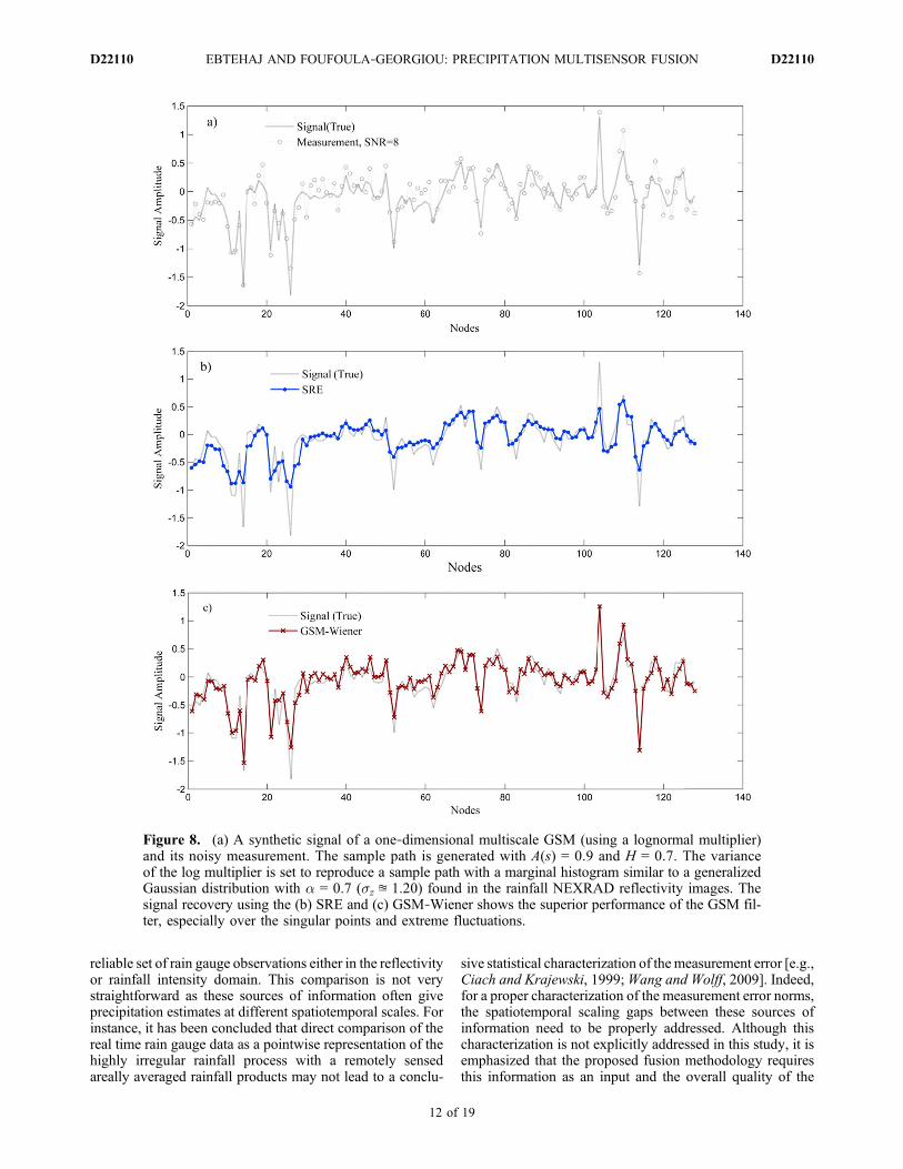
signal is considered as the true values which have to berecovered, given a set of noisy observations y(s) = d(s) + v(s),where v(s) ∼ N (0, Sv(s)). For this particular case of one‐dimensional simulation, the signal‐to‐noise ratio, was set onthe order of 8 dB to generate the noisy measurements. Toexploit the multiscale structure of the process, the general-ized neighborhood includes a single reference point of theprocess and only a single parent node in the next coarserscale; i.e.,Su is a 2 × 2 matrix. This allows us to incorporate alocal scale‐to‐scale correlation (see, e.g., Figure 2) and cap-ture the parent and child dynamics, for improving the signalrecovery. A realization of this synthetic simulation and therecovered signal, using the standard linear multiscale esti-mation (SRE) and the local GSM‐Wiener filter is presentedin Figure 8 for the seventh scale level on a dyadic treewith 27 leaf nodes. Qualitatively, the GSM‐Wiener is out-performing the SRE method especially over the recovery ofthe peaks and singularities. Note that for both cases, theestimation process suppresses the noise over the regionswhere the signal is of low amplitude; however, the GSM‐Wiener filter shows a better performance over the singularpoints. This can also be quantitatively evaluated in terms ofsome vector norms of error; i.e., kekp. A normalized mea-sure ðkeskp�keGkpÞ=keSkp is defined, where keSkp and keGkp arethe p‐norms of the error for the recovered signal using SREand GSM‐Wiener filters, respectively. For instance, in thisparticular case, assuming p = 2, the 2‐norm (energy) of erroris improved about 20 percent while this gain rose to about45 percent for the infinity norm or the maximum absolutevalue of the error vector. This significant improvementimplies that GSM‐Wiener filtering can outperform standardGaussian methods on the recovery of the commonly observedtypes of singularities in the precipitation fields, while alsokeeping the other common norms of the error even lower thanthe standard linear estimation algorithms.[42] Analogous to the explained one‐dimensional case, it

is expected that estimating multisensor precipitation datausing standard linear Gaussian filtering methods such as theSRE, may result in not properly capturing important sin-gular features of the fields which can potentially be of greathydrometeorological importance.

6. GSM Multisensor Fusion of Precipitation Data

6.1. Conceptual Development

[43] In this section we describe how the explained GSM‐Wiener filter can be employed for optimal estimation andfusion of the precipitation reflectivity images, given differ-ent sources of noisy observations. It has long been recog-nized that all of the active and passive precipitation sensorshave their own specific measurement error structure [see, e.g.,Wang and Wolff, 2009]. As explained previously, in recentdecades significant effort has been devoted to error charac-terization of the remotely sensed precipitation products.Typically, using an appropriate Z‐R relationship, this involvesstatistical comparison of the remotely sensed data with a


11 of 19

reliable set of rain gauge observations either in the reflectivityor rainfall intensity domain. This comparison is not verystraightforward as these sources of information often giveprecipitation estimates at different spatiotemporal scales. Forinstance, it has been concluded that direct comparison of thereal time rain gauge data as a pointwise representation of thehighly irregular rainfall process with a remotely sensedareally averaged rainfall products may not lead to a conclu-

sive statistical characterization of themeasurement error [e.g.,Ciach and Krajewski, 1999;Wang and Wolff, 2009]. Indeed,for a proper characterization of the measurement error norms,the spatiotemporal scaling gaps between these sources ofinformation need to be properly addressed. Although thischaracterization is not explicitly addressed in this study, it isemphasized that the proposed fusion methodology requiresthis information as an input and the overall quality of the

Figure 8. (a) A synthetic signal of a one‐dimensional multiscale GSM (using a lognormal multiplier)and its noisy measurement. The sample path is generated with A(s) = 0.9 and H = 0.7. The varianceof the log multiplier is set to reproduce a sample path with a marginal histogram similar to a generalizedGaussian distribution with a = 0.7 (sz ≊ 1.20) found in the rainfall NEXRAD reflectivity images. Thesignal recovery using the (b) SRE and (c) GSM‐Wiener shows the superior performance of the GSM fil-ter, especially over the singular points and extreme fluctuations.


12 of 19

fusion process highly depends on this error characterization.Note that the proposed fusion methodology is just a filteringmethod to estimate the conditional expectation of the unbi-ased noisy precipitation data. Therefore, it is also assumedthat there is no systematic bias in the observation instrumentsand any sort of bias adjustment has to be performed prior toapplying the presented fusion algorithm.[44] To address the scaling issues involved in precipita-

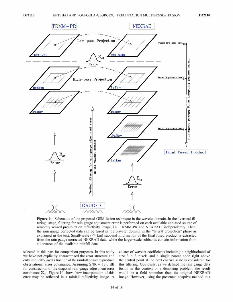
tion multisensor estimation, the new proposed fusion meth-odology possesses a multiscale filtering structure. Practicalimplementation of this methodology does not necessarilyrequire a stochastic or physically based precipitation modelto fill the scaling gaps between the available high‐resolution(NEXRAD) and low‐resolution (TRMM‐PR) precipitationproducts. Indeed, as the estimation process is performed in apyramidal data structure in the wavelet domain, in the pre-sented case study, the high‐resolution (i.e., <4 km) infor-mation of the final fused product would be solely based onthe rain gauge corrected NEXRAD wavelet coefficients.However, in the scales where the TRMM data are alsoavailable; i.e., ≥4 km, the fusion process exploits all sourcesof information (see Figure 9).[45] Basically, by comparing different sources of rainfall

measurements, three different error covariance matricesneed to be characterized for proper implementation of theproposed fusion technique: (1) Sv1, NEXRAD versus raingauges; (2)Sv2, TRMM‐PR versus rain gauges; and (3)Sv3,NEXRAD versus TRMM‐PR. Hereafter, the error covar-iances Sv1 and Sv2 are called “rain gauge adjustment error.”Note that although the results of the fusion process will bemore complete using all of the error covariance information,lack of knowledge about any of these error matrices is notprohibitive for practical implementation of the introducedmethodology. This becomes more clear as we proceed toelaborate the method in detail.[46] The proposed GSM multisensor multiscale method-

ology consists of twomajor steps namely “Vertical Filtering”and “Lateral Projection” (see Figure 9). In the vertical fil-tering phase, incorporation of the measurement errors isconsidered as a filtering problem of the sort y = x + v,where y denotes the remotely sensed precipitation obser-vation and x is the true precipitation process which is cor-rupted by a Gaussian noise v. Substituting Sv1 and Sv2 aserror covariance matrices in equation (11), the rain gaugeadjustment errors are first filtered out from the wavelet high‐pass subbands of the TRMM and NEXRAD data, indepen-dently. Afterwards, in the scales where both the TRMM andNEXRAD data become available (i.e., ≥4 km), given thecharacterized error covariance Sv3, the rain gauge correctedsubband information of the TRMM images can be laterallyprojected at the same scales onto the subspace spanned by therain gauge corrected subbands of the NEXRAD measure-ments. For the scales, where the TRMM‐PR data are notavailable (i.e., <4 km) the high‐pass subband information ofthe fused product will be solely obtained from the rain gaugecorrected NEXRADwavelet coefficients. At the last step, theerror corrected wavelet coefficients at all scales are used toreconstruct the final fused product using the inverse wavelettransform (see Figure 9).[47] Theoretically speaking, using equation (11) in lateral

projection phase, we can keep decomposing the observations(i.e., TRMM and NEXRAD) into multiple levels until we end

up with a single valued low‐pass subband and performingthe GSM fusion on the high‐pass coefficients over all thescales where the data from both sensors are available. Thisprocedure might be computationally expensive and it seemsreasonable to perform finite levels of the wavelet decom-position for fusion and denoising purposes, knowing thathigh‐frequency noisy features of a signal are typicallycaptured at the first levels of wavelet high‐pass coefficients.Consequently, at a certain scale level, we eventually need toproject the nonzero mean low‐pass coefficients of the low‐resolution products (TRMM) onto the similar subspace (samescale) spanned by the high‐resolution data (NEXRAD).As the non‐Gaussian features of the signals are typicallycaptured in high‐pass subbands in the wavelet domain [seeEbtehaj and Foufoula‐Georgiou, 2011], the low‐pass coef-ficients can be fused using a conventional least squares for-malism as expressed in equations (1) and (2),

E xljyl½ � � mxl þSxl Sxl þSv3ð Þ�1 yl � myl

� �; ð13Þ

where yl,myl denote the NEXRAD low‐pass coefficients andtheir mean in a local spatial neighborhood; andmxl,Sxl are theaverage and covariance of the TRMM low‐pass coefficientsin that neighborhood, respectively. Obviously, as there isno lower‐scale subband information available while fusinglow‐pass coefficients, the neighborhoods in this case justinclude a cluster of coefficients in a single subband and thereis no information of parent nodes encoded in the covariancematrices of equation (13).[48] Besides the input error covariances, a set of two

parameters need to be determined in the presented fusionmethodology, including: (1) the structure and size of thegeneralized neighborhood and (2) the levels of the waveletdecomposition. In this work, we did not perform a quantita-tive assessment of different choices of the parameters on thefusion results and simply chose values we found empiricallyto perform well.[49] As explained previously, the correlation of the rain-

fall wavelet coefficients almost vanishes over a neighbor-hood of size 3 to 5 pixels (km) for the first level of subbandcoefficients. In general, it is found that increasing the sizeof the neighborhood (i.e., enlarging the estimated correlationdomain) gives rise to a smoother and more blurred fusionproduct. On the other hand, smaller spatial neighborhoodsgenerally generate a product which contains sharper andmore detailed structure of the high‐intensity rain cells.[50] It is also observed that over the decomposition levels

2–4 (i.e., 4–16 km) the noise (observational error) can bewell captured in the wavelet domain and the results ofthe fusion are satisfactory. Of course, for higher levels ofdecomposition the low‐pass fusion takes place at largerscales which means that more detailed features of the fusedproduct will be obtained from the higher‐resolution data(e.g., NEXRAD) and incorporation of small‐scale informa-tion of the low‐resolution sensor (e.g., TRMM‐PR) wouldbe less significant.

6.2. A Case Study on Precipitation Data

[51] The TRMM‐PR and NEXRAD coincidental reflec-tivity image of a storm on 28 June 1998 over the HSTN site,used for the SRE implementation (see section 3.2), is also


13 of 19

selected in this part for comparison purposes. In this studywe have not explicitly characterized the error structure andonly implicitly used a fraction of the rainfall power to produceobservational error covariance. Assuming SNR = 13.0 dBfor construction of the diagonal rain gauge adjustment errorcovariance Sv1, Figure 10 shows how incorporation of thiserror may be reflected in a rainfall reflectivity image. A

cluster of wavelet coefficients including a neighborhood ofsize 3 × 3 pixels and a single parent node right abovethe central point at the next coarser scale is considered forthis filtering. Obviously, as we defined the rain gauge datafusion in the context of a denoising problem, the resultwould be a field smoother than the original NEXRADimage. However, using the presented adaptive method this

Figure 9. Schematic of the proposed GSM fusion technique in the wavelet domain. In the “vertical fil-tering” stage, filtering for rain gauge adjustment error is performed on each available unbiased source ofremotely sensed precipitation reflectivity image, i.e., TRMM‐PR and NEXRAD, independently. Then,the rain gauge corrected data can be fused in the wavelet domain in the “lateral projection” phase asexplained in the text. Small‐scale (<4 km) subband information of the final fused product is extractedfrom the rain gauge corrected NEXRAD data, while the larger‐scale subbands contain information fromall sources of the available rainfall data.


14 of 19

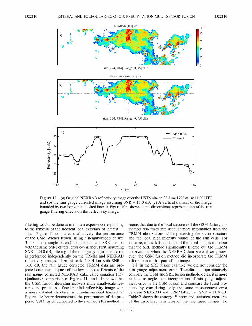
filtering would be done at minimum expense correspondingto the removal of the frequent local extremes of interest.[52] Figure 11 compares qualitatively the performance

of the GSM‐Wiener fusion (using a neighborhood of size3 × 3 plus a single parent) and the standard SRE methodwith the same order of total error covariance. First, assumingSNR = 24.0 dB, filtering of the rain gauge adjustment erroris performed independently on the TRMM and NEXRADreflectivity images. Then, at scale 4 × 4 km with SNR =16.0 dB, the rain gauge corrected TRMM data are pro-jected onto the subspace of the low‐pass coefficients of therain gauge corrected NEXRAD data, using equation (13).Qualitative comparison of Figures 11a and 11b shows thatthe GSM fusion algorithm recovers more small‐scale fea-tures and produces a fused rainfall reflectivity image witha more detailed structure. A one‐dimensional transect inFigure 11c better demonstrates the performance of the pro-posed GSM fusion compared to the standard SRE method. It

seems that due to the local structure of the GSM fusion, thismethod also takes into account more information from theTRMM observations while preserving the storm structureand the local high‐intensity values of the rain cells. Forinstance, in the left‐hand side of the fused images it is clearthat the SRE method significantly filtered out the TRMMobservations when the NEXRAD data were absent; how-ever, the GSM fusion method did incorporate the TRMMinformation in that part of the image.[53] In the SRE fusion example we did not consider the

rain gauge adjustment error. Therefore, to quantitativelycompare the GSM and SRE fusion methodologies, it is morerealistic to neglect the incorporation of rain gauge adjust-ment error in the GSM fusion and compare the fused pro-ducts by considering only the same measurement errorbetween NEXRAD and TRMM‐PR; i.e., SNR = 11.0 dB.Table 2 shows the entropy, F‐norm and statistical measuresof the associated rain rates of the two fused images. To

Figure 10. (a) Original NEXRAD reflectivity image over the HSTN site on 28 June 1998 at 18:13:00UTCand (b) the rain gauge corrected image assuming SNR = 13.0 dB. (c) A vertical transect of the image,bounded by two horizontal dashed lines in Figure 10b, shows a one‐dimensional representation of the raingauge filtering effects on the reflectivity image.


15 of 19

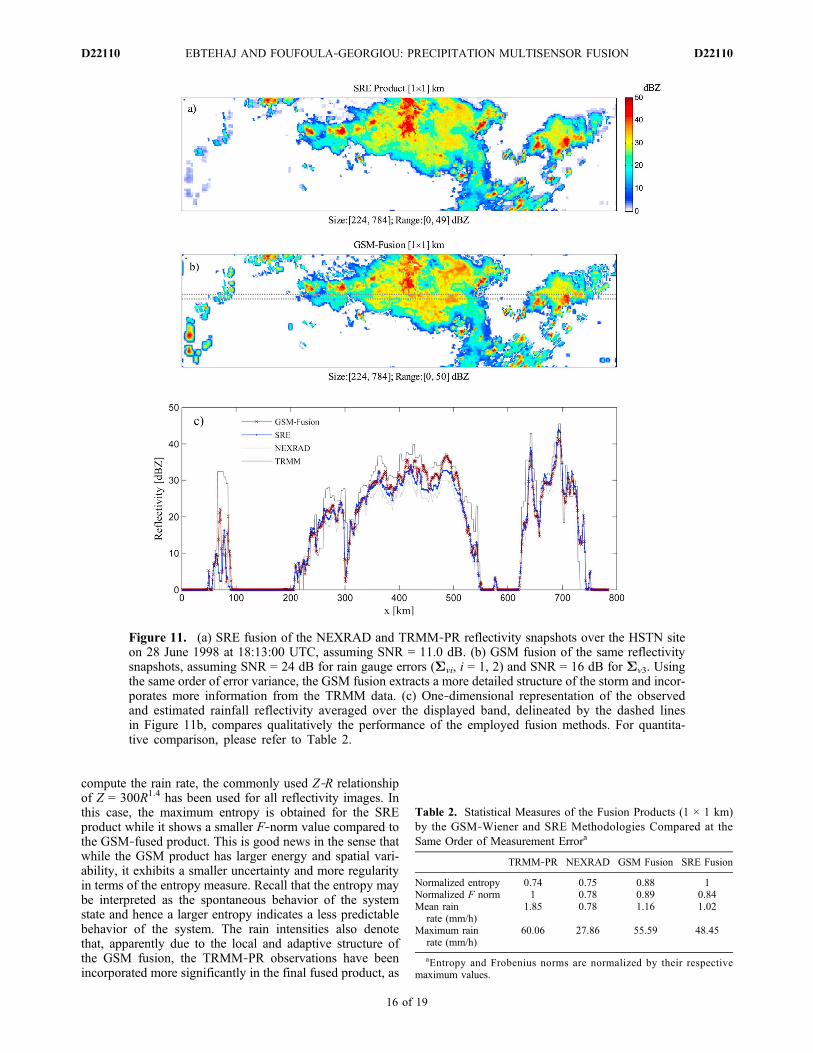
compute the rain rate, the commonly used Z‐R relationshipof Z = 300R1.4 has been used for all reflectivity images. Inthis case, the maximum entropy is obtained for the SREproduct while it shows a smaller F‐norm value compared tothe GSM‐fused product. This is good news in the sense thatwhile the GSM product has larger energy and spatial vari-ability, it exhibits a smaller uncertainty and more regularityin terms of the entropy measure. Recall that the entropy maybe interpreted as the spontaneous behavior of the systemstate and hence a larger entropy indicates a less predictablebehavior of the system. The rain intensities also denotethat, apparently due to the local and adaptive structure ofthe GSM fusion, the TRMM‐PR observations have beenincorporated more significantly in the final fused product, as

Figure 11. (a) SRE fusion of the NEXRAD and TRMM‐PR reflectivity snapshots over the HSTN siteon 28 June 1998 at 18:13:00 UTC, assuming SNR = 11.0 dB. (b) GSM fusion of the same reflectivitysnapshots, assuming SNR = 24 dB for rain gauge errors (Svi, i = 1, 2) and SNR = 16 dB for Sv3. Usingthe same order of error variance, the GSM fusion extracts a more detailed structure of the storm and incor-porates more information from the TRMM data. (c) One‐dimensional representation of the observedand estimated rainfall reflectivity averaged over the displayed band, delineated by the dashed linesin Figure 11b, compares qualitatively the performance of the employed fusion methods. For quantita-tive comparison, please refer to Table 2.

Table 2. Statistical Measures of the Fusion Products (1 × 1 km)by the GSM‐Wiener and SRE Methodologies Compared at theSame Order of Measurement Errora

TRMM‐PR NEXRAD GSM Fusion SRE Fusion

Normalized entropy 0.74 0.75 0.88 1Normalized F norm 1 0.78 0.89 0.84Mean rain

rate (mm/h)1.85 0.78 1.16 1.02

Maximum rainrate (mm/h)

60.06 27.86 55.59 48.45

aEntropy and Frobenius norms are normalized by their respectivemaximum values.


16 of 19

the GSM product shows a larger mean and larger maximumvalues compared to the SRE method (see Figure 11c).Knowing that the wetted area in the studied storm snapshotis about 120 × 103 km2, the difference between the esti-mated rain budget from the original and fused productsseems significant which denotes the importance of the pre-cipitation fusion. The precipitation products that we haveused in this study might not be the best from an operationalstandpoint and to substantiate more the practical benefits ofthe proposed precipitation fusion methodology, these find-ings need to be further investigated and solidified by moredetailed analysis of other storm cases for which “groundtruth” highly accurate rain gauge data are available.

7. Conclusion

[54] A new method is presented which allows us to inte-grate multiscale multiplatform precipitation measurements toprovide a posteriori estimates of spatial rainfall. This methodexploits the multiscale representation of precipitation imagesin the wavelet domain and specifically a particular class ofGaussian‐scale mixture (GSM) distributions as the proba-bility model of the wavelet high‐pass coefficients of rainfalldata. This algorithm is structured in a way that it can addressthe non‐Gaussian statistics and capture the extreme inten-sity values of the precipitation fields in a Gaussian noiseenvironment with a superior performance and many otheradvantages compared to the commonly used standard lin-ear Gaussian fusion techniques. Exploiting the decorrelatingeffects of the wavelet decomposition, the posteriori estimatesrely on the local multiscale spatial covariance structure ofthe rainfall fields in the wavelet domain. Therefore, as thewavelet decomposition converts a strongly correlated fieldinto a set of weakly correlated subbands, in lieu of estimat-ing the entire covariance of the original field in the spatialdomain, a local representation of the covariance is estimatedin each subband and used for optimal estimation and fusion.This makes the problem computationally more efficient whileallowing to capture the non‐Gaussian marginal statistics ofthese fields. Depending on the typical rainfall domain sizefor a single NEXRAD station and without any special opti-mization in coding style, running the MATLAB code of thealgorithm on an Intel(R)‐i7CPU with 2.80 GHz clock rate,takes in the order of less than 5 min.[55] Using the developed fusion methodology, we can

obtain a posteriori estimates of rainfall images as long asground‐based and spaceborne precipitation data are coinci-dentally available. Therefore, according to the revisitingtime of the TRMM satellite or other sources of spaceborneprecipitation data, we could update the satellite reflectivityimages all over the contiguous United States using thenational NEXRADmosaic images. The fused rainfall productin this sense can be used in data assimilation systems toimprove forecasts at the local and regional scales. Applica-bility of the developed methodology for obtaining posterioriestimates of spatial rainfall fields, given TRMM MicrowaveImager (TMI) rainfall information, seems feasible and mightbe of great interest for future development of this work. Itis worth nothing that, this fusion methodology can also beapplied to rainfall data at different time scales (e.g., daily ormonthly data), as long as the error covariance is properly

determined for that specific time scale. However, for larger‐scale cumulative precipitation data the non‐Gaussian sig-nature is naturally less significant.[56] Due to the local structure of the proposed estimation

or fusion methodology, the range dependence effects of thesensors can also be easily incorporated in the error covari-ance matrices. This might be of great interest for estimationand fusion of the orbital satellite products produced by crosstrack instruments, where the measurement error shows asystematic dependence on the distance of the detected pre-cipitation with respect to the centerline of the swath (e.g.,Advanced Microwave Sounding Unit). Furthermore, in abroader context, applicability of the GSM probability modelfor data assimilation of non‐Gaussian large‐scale geophys-ical processes (e.g., soil moisture, atmospheric state vari-ables) could also be of great interest for future research.Obviously, developing efficient algorithms in this contextcan significantly improve the shortcomings of the conven-tional Gaussian‐based assimilation methods with respect tothe typically observed extremes and singularities of interestin natural processes.

Appendix A: Details of Some DerivationsA1. Maximum a Posteriori Estimate of the LognormalMultiplier

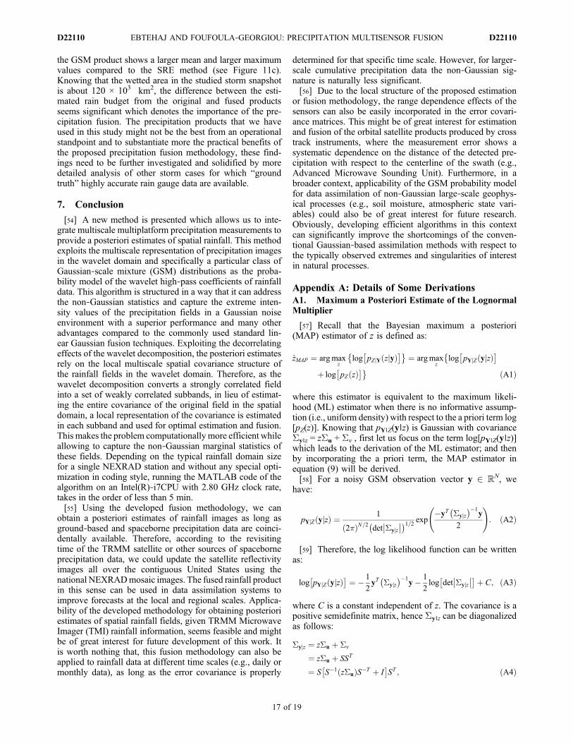
[57] Recall that the Bayesian maximum a posteriori(MAP) estimator of z is defined as:

zMAP ¼ argmaxz

log pZjY zjyð Þ� �

¼ argmaxz

log pYjZ yjzð Þ�

þ log�pZ zð Þ

�ðA1Þ

where this estimator is equivalent to the maximum likeli-hood (ML) estimator when there is no informative assump-tion (i.e., uniform density) with respect to the a priori term log[pZ(z)]. Knowing that pY∣Z(y∣z) is Gaussian with covarianceSy∣z = zSu + Sv , first let us focus on the term log[pY∣Z(y∣z)]which leads to the derivation of the ML estimator; and thenby incorporating the a priori term, the MAP estimator inequation (9) will be derived.[58] For a noisy GSM observation vector y 2 RN, we

have:

pYjZ yjzð Þ ¼ 1

2�ð ÞN=2 det Syjz�� 1=2 exp �yT Syjz

� ��1y

2

!: ðA2Þ

[59] Therefore, the log likelihood function can be writtenas:


¼ � 1

2yT Syjz� ��1

y� 1

2log det Syjz

�� þ C; ðA3Þ

where C is a constant independent of z. The covariance is apositive semidefinite matrix, hence Sy∣z can be diagonalizedas follows:

Syjz ¼ zSu þ Sv

¼ zSu þ SST

¼ S S�1 zSuð ÞS�T þ I�

ST ; ðA4Þ


17 of 19

where S is the square root of Sv = SST which can be com-puted using Cholesky or eigenvalue decomposition. Notethat S−1SuS

−T is also a symmetric positive semidefinitematrix, which can be diagonalized by an eigenvalue decom-position (i.e., spectral factorization) as S−1SuS

−T = QLQT,where {Q, L} are matrices containing orthogonal eigenvec-tors QQT = I and positive eigenvalues ln 2 L, respectively.Therefore, diagonalization in equation (A4) can be writtenas:

Syjz ¼ SQ zLþ Ið ÞQTST : ðA5Þ

[60] Using this diagonalized version of the covariancematrix, equation (A3) can be further expanded as follows:


¼ � 1

2yT SQ zLþ Ið ÞQTST� ��1

y

� 1

2log det SQ zLþ Ið ÞQTST

�� þ C

¼ � 1

2QTS�1y� �T

zLþ Ið Þ�1 QTS�1y� �

� 1

2log det SQ zLþ Ið ÞQTST

�� þ C

¼ � 1

2VT zLþ Ið Þ�1V � 1

2log det zLþ Ij j½ � þ C′;

ðA6Þ

where the vector V = QTS−1y. Note that zL + I is a diagonalmatrix whose determinant is equal to the multiplicationof its diagonal elements {zln + 1}n=1

N . Therefore, takingderivative of equation (A6) with respect to z, we have:

@ log pYjZ yjzð Þ� @z

¼ 1

2VT L zLþ Ið Þ�2� �

V � 1

2

XNn¼1

�n

z�n þ 1

¼ 1

2

XNn¼1

�nv2nz�n þ 1ð Þ2

� 1

2

XNn¼1

�n

z�n þ 1

¼ 1

2

XNn¼1

��1n v2n � 1� �

� z

zþ ��1n

� �2 : ðA7Þ

[61] Note that assuming a noninformative density for themultiplier, setting equation (A7) equal to zero, the root givesthe maximum likelihood estimator of z.[62] Assuming a lognormal density pZ(z; mz, sz) = 1

zffiffiffiffi2�

p�z

exp (� logz�zð Þ22�2z

), the derivative of the log likelihood is thengiven by:

log pZ zð Þ½ � ¼ � log z� zð Þ2

2�2z

� log zð Þ þ C ðA8Þ

@ log pZ zð Þ½ �@z

¼ � log zþ z � �2z

z�2z

: ðA9Þ

[63] Then combining equations (A7) and (A9), leads tothe derivation of equation (9):

log zMAP þ 32�

2z

zMAP�2z

þ 1

2

XNn¼1

zMAP � ��1n v2n � 1� �

zMAP þ ��1n

� �2 ¼ 0: ðA10Þ

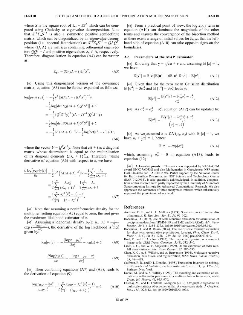
[64] From a practical point of view, the log zMAP term inequation (A10) can dominate the magnitude of the otherterms and ensures the convergence of the bisection methodas there exists a range of initial values for zMAP, that the left‐hand side of equation (A10) can take opposite signs on theboundaries.

A2. Parameters of the MAP Estimator

[65] Knowing that y =ffiffiz

pu + v and assuming E [z] = 1,

we have:

E y4�

¼ E z2�

E u4�

þ 6E u2�

E v2�

þ E v4�

: ðA11Þ

[66] Given that for the zero mean Gaussian distributionE [u4] = 3su

4 and E [v4] = 3sv4 leads to:

E z2�

¼ E y4½ �=3� 2�2u�

2v � �4

v

�4u

: ðA12Þ

[67] As su2 = sy

2 − sv2, equation (A12) can be updated to:

E z2�

¼E y4½ �=3� 2�2

y�2v þ �4

v

�2y � �2

v

� �2 : ðA13Þ

[68] As we assumed z is LN (mz, sz) with E [z] = 1, wehave mz + 1

2sz2 = 1, hence:

E z2�

¼ exp �2z

� �; ðA14Þ

which, assuming sv2 = 0 in equation (A13), leads to

equation (12).

[69] Acknowledgments. This work was supported by NASA‐GPMaward NNX07AD33G and also Mathematics in Geosciences NSF grantsEAR‐0824084 and EAR‐0835789. Partial support by the National Centerfor Earth‐Surface Dynamics, an NSF Science and Technology Center(EAR‐0120914), is also gratefully acknowledged. In addition, computa-tions of this research were partly supported by the University of MinnesotaSupercomputing Institute for Advanced Computational Research. We alsoappreciate the comments of three anonymous referees which substantiallyimproved the presentation of our work.

ReferencesAndrews, D. F., and C. L. Mallows (1974), Scale mixtures of normal dis-tributions, J. R. Stat. Soc., Ser. B., 36, 99–102.

Bocchiola, D. (2007), Use of scale recursive estimation for assimilation ofprecipitation data from TRMM (PR and TMI) and NEXRAD, Adv. WaterResour., 30(11), 2354–2372, doi:10.1016/j.advwatres.2007.05.012.

Bocchiola, D., and R. Rosso (2006), The use of scale recursive estimationfor short term quantitative precipitation forecast, Phys. Chem. Earth,Parts A, B, C, 31(18), 1228–1239, doi:10.1016/j.pce.2006.03.019.

Burt, P., and E. Adelson (1983), The Laplacian pyramid as a compactimage code, IEEE Trans. Commun., 31(4), 532–540.

Ciach, J. G., and W. F. Krajewski (1999), On the estimation of radar rain-fall error variance, Adv. Water Resour., 22, 585–595.

Chou, K. C., A. S. Willsky, and A. Benveniste (1994), Multiscale recursiveestimation, data fusion, and regularization, IEEE Trans. Autom. Control,39, 464–478.

Coifman, R. R., and D. L. Donoho, (1995), Translation‐invariant de‐noising,in Wavelets and Statistics, Lecture Notes Stat., vol. 103, pp. 125–150,Springer, New York.

Daniel, M., and A. S. Willsky (1999), The modeling and estimation of sta-tistically self‐similar processes in a multiresolution framework, IEEETrans. Inf. Theory, 45, 955–970.

Ebtehaj, M., and E. Foufoula‐Georgiou (2010), Orographic signature onmultiscale statistics of extreme rainfall: A storm‐scale study, J. Geophys.Res., 115, D23112, doi:10.1029/2010JD014093.


18 of 19

Ebtehaj, M., and E. Foufoula‐Georgiou (2011), Statistics of precipitationreflectivity images and cascade of Gaussian‐scale mixtures in the waveletdomain: A formalism for reproducing extremes and coherent multiscalestructures, J. Geophys. Res., 116, D14110, doi:10.1029/2010JD015177.

Fristedt, B., N. Jain, and N. Krylov (2007), Filtering and Prediction: APrimer, Student Math. Libr., vol. 8, 252 pp., Am. Math. Soc., Providence,R. I.

Gonzalez, R. C., and R. E.Woods (2008),Digital Image Processing, 3rd ed.,954 pp., Prentice Hall, Upper Saddle River, N. J.

Gorenburg, I. P., D. McLaughlin, and D. Entekhabi (2001), Scale‐recursiveassimilation of precipitation data, Adv. Water Resour., 24(9‐10), 941–953,doi:10.1016/S0309-1708(01)00033-1.

Gupta, V. K., and E. C. Waymire (1993), A statistical analysis of mesoscalerainfall as a random cascade, J. Appl. Meteorol., 32, 251–267.

Gupta, R., V. Venugopal, and E. Foufoula‐Georgiou (2006), A methodol-ogy for merging multisensor precipitation estimates based on expecta-tion‐maximization and scale‐recursive estimation, J. Geophys. Res.,111, D02102, doi:10.1029/2004JD005568.

Kalman, R. (1960), A new approach to linear filtering and prediction pro-blems, J. Basic Eng., 82, 35–45.

Krajewski, W. F., and J. A. Smith (2002), Radar hydrology: Rainfall esti-mation, Adv. Water Resour., 25(8–12), 1387–1394, doi:10.1016/S0309-1708(02)00062-3.

Kumar, P. (1999), A multiple scale state‐space model for characterizingsubgrid scale variability of near‐surface soil moisture, IEEE Trans.Geosci. Remote Sens., 37, 182–197.

LeCam, L. (1961), A stochastic description of precipitation, in Proceedingsof the Fourth Berkeley Symposium onMathematical Statistics and Probabil-ity, vol. 4, Biology and Problems of Health, vol. 4, edited by J. Neyman,pp. 165–186, Univ. of Calif. Press, Berkeley.

Levy, B. C. (2008), Principles of Signal Detection and Parameter Estima-tion, 639 pp., Springer, New York.

Lovejoy, S., and D. Schertzer (1990), Multifractals, universality classes andsatellite and radar measurements of clouds and rain fields, J. Geophys.Res., 95(D3), 2021–2034.

Luettgen, M. R., W. C. Karl, A. S. Willsky, and R. R. Tenney (1993), Multi-scale representations ofMarkov random fields, IEEETrans. Signal Process.,41, 3377–3396.

Menabde, M., D. Harris, A. Seed, G. Austin, and D. Stow (1997), Multi-scaling properties of rainfall and bounded random cascades, WaterResour. Res., 33(12), 2823–2830, doi:10.1029/97WR02006.

Nadarajah, S. (2005), A generalized normal distribution, J. Appl. Stat., 32(7),685–694.

Nason, G. P., and B. W. Silverman (1995), The stationary wavelet trans-form and some statistical applications, in Wavelets and Statistics, LectureNotes Stat., vol. 103, pp. 281–299, Springer, New York.

Portilla, J., V. Strela, M. Wainwright, and E. Simoncelli (2001), AdaptiveWiener denoising using a Gaussian scale mixture model in the waveletdomain, in Proceedings of 2001 International Conference on Image Pro-cessing, pp. 37–40, IEEE Press, New York.

Portilla, J., V. Strela, M. J. Wainwright, and E. P. Simoncelli (2003), Imagedenoising using scale mixtures of Gaussians in the wavelet domain, IEEETrans. Image Process., 12(11), 1338–1351.

Rauch, H., F. Tung, and C. Strieble (1965), Maximum likelihood estimatesof linear dynamic systems, AIAA J., 3(8), 1445–1450.

Strela, V. (2000), Denoising via block Wiener filtering in wavelet domain,in Proceedings of the Third European Congress of Mathematics, vol. 2,Birkhäuser, Basel, Switzerland.

Strela, V., J. Portilla, and E. Simoncelli (2000), Image denoising using alocal Gaussian scale mixture model in the wavelet domain, paper pre-sented at SPIE Conference on Wavelet Applications in Signal and ImageProcessing, Int. Soc. for Opt. Eng., San Diego, Calif.

Tustison, B., E. Foufoula‐Georgiou, and D. Harris (2002), Scale‐recursiveestimation for multisensor quantitative precipitation forecast verification:A preliminary assessment, J. Geophys. Res., 107(D8), 8377, doi:10.1029/2001JD001073.

Van de Vyver, H., and E. Roulin (2009), Scale recursive estimation formerging precipitation data from radar and microwave cross track scan-ners, J. Geophys. Res., 114, D08104, doi:10.1029/2008JD010709.

Wainwright, M. J., and E. P. Simoncelli (2000), Scale mixtures of Gaus-sians and the statistics of natural images, Adv. Neural Inf. Process. Syst.,12, 855–861.

Wainwright, M. J., E. P. Simoncelli, and A. S. Willsky (2001), Randomcascades on wavelet trees and their use in analyzing and modeling naturalimages, Appl. Comput. Harmonic Anal., 11, 89–123.

Wang, J., and D. B. Wolff (2009), Evaluation of TRMM ground‐validationradar‐rain errors using rain gaugemeasurements, J. Appl.Meteorol. Climatol.,49(2), 310–324, doi:10.1175/2009JAMC2264.

West, M. (1987), On scale mixtures of normal distributions, Biometrika,74(3), 646–648.

Willsky, A. S. (2002), Multiresolution Markov models for signal and imageprocessing, Proc. IEEE, 90, 1396–1458.

Wornell, G. W. (1990), A Karhunen‐Loève‐like expansion for 1/f pro-cesses via wavelets, IEEE Trans. Inf. Theory, 36, 859–861.

A.M. Ebtehaj and E. Foufoula‐Georgiou, Saint Anthony Falls Laboratory,Department of Civil Engineering, University of Minnesota, Twin Cities, 2Third Ave. SE, Minneapolis, MN 55414‐2196, USA. ([email protected])


19 of 19

adaptive fusion of multisensor precipitation using …efi.eng.uci.edu/papers/efg_113.pdf · ·...

Documents