adaptive finite element methods lecture 2: a posteriori ... · outline model problem a posteriori...

Adaptive Finite Element MethodsLecture 2: A Posteriori Error Estimation

Ricardo H. Nochetto

Department of Mathematics andInstitute for Physical Science and Technology

University of Maryland, USA

www.math.umd.edu/˜rhn

School - Fundamentals and Practice of Finite ElementsRoscoff, France, April 16-20, 2018

Outline Model Problem A Posteriori Error Analysis H−1 Data Role of Oscillation Surveys

Outline

Model Problem and FEM

FEM: A Posteriori Error Analysis

Dealing with H−1 Data (Cohen, DeVore, N’ 12)

Role of Oscillation Revisited (Kreuzer, Veeser’ 18)

Surveys

Adaptive Finite Element Methods Lecture 2: A Posteriori Error Estimation Ricardo H. Nochetto

Outline

Surveys

Model Problem: Basic Assumptions

Consider model problem

−div(A∇u) = f in Ω, u|∂Ω = 0,

with

I Ω polygonal domain in Rd, d ≥ 2;

I T0 is a conforming mesh made of simplices with compatible labeling;

I A(x) is symmetric and positive definite for all x ∈ Ω with eigenvalues λ(x)satisfying

0 < amin ≤ λi(x) ≤ amax, x ∈ Ω;

I A is piecewise Lipschitz in T0;

I f ∈ L2(Ω) (and f ∈ H−1(Ω) later in Lecture 2);

I V(T ) space of continuous elements of degree ≤ n over a conformingrefinement T of T0 (by bisection).

I Exact numerical integration.

Page 5: Adaptive Finite Element Methods Lecture 2: A Posteriori ... · Outline Model Problem A Posteriori Error Analysis H 1 Data Role of Oscillation Surveys A Priori Error Analysis If u2A

Galerkin Method

I Function space: V := H10 (Ω).

I Bilinear form: B : V× V→ R

B(v, w) :=

∫Ω

A∇v · ∇w ∀v, w ∈ V.

Then solution u of model problem satisfies

u ∈ V : B(u, v) = 〈f, v〉 ∀v ∈ V.

I Finite element space: If Pn(T ) denote polynomials of degree ≤ n overT , then

V(T ) := v ∈ H10 (Ω) : v|T ∈ Pn(T ) ∀T ∈ T .

I Galerkin solution: The discrete solution U = UT satisfies

U ∈ V(T ) : B(U, V ) = 〈f, V 〉 ∀V ∈ V(T ).

Page 6: Adaptive Finite Element Methods Lecture 2: A Posteriori ... · Outline Model Problem A Posteriori Error Analysis H 1 Data Role of Oscillation Surveys A Priori Error Analysis If u2A

Galerkin Method (Continued)

I Residual: R ∈ V ∗ = H−1(Ω) is given by

〈R, v〉 := 〈f, v〉 − B(U, v) = B(u− U, v) ∀v ∈ V.

I Galerkin Orthogonality:

〈R, V 〉 = 〈f, V 〉 − B(U, V ) ∀V ∈ V(T ).

I Quasi-Best Approximation (Cea Lemma): Let α1 ≤ α2 be the coercivityand continuity constants of B

α1‖u− U‖2V ≤ B(u− U, u− U) = B(u− U, u− V )

≤ α2‖u− U‖V‖u− V ‖V ∀V ∈ V(T ).

⇒ ‖u− U‖V ≤α2

α1inf

V ∈V(T )‖u− V ‖V.

I Approximation Class As: Let 0 < s ≤ n/d (n ≥ 1) and

As :=v ∈ V : |v|s := sup

N>0

(Ns inf

#T −#T0≤Ninf

V ∈V(T )‖v − V ‖V

)⇒ ∃ T ∈ T : #T −#T0 ≤ N, inf

V ∈V(T )‖v − V ‖V ≤ |v|sN−s.

Page 7: Adaptive Finite Element Methods Lecture 2: A Posteriori ... · Outline Model Problem A Posteriori Error Analysis H 1 Data Role of Oscillation Surveys A Priori Error Analysis If u2A

A Priori Error Analysis

If u ∈ As, 0 < s ≤ n/d, there exists T ∈ T with #T −#T0 ≤ N and

‖u− U‖V ≤α2

α1|u|sN−s.

I If n = 1, d = 2, p > 1, and u ∈ V ∩W 2p (Ω; T0), then GREEDY shows that

|u|1/2 4 ‖D2u‖Lp(Ω;T0) whence (optimal estimate)

∃ T ∈ T : #T −#T0 ≤ N, ‖u− U‖V 4 ‖D2u‖Lp(Ω;T0)N−1/2.

I GREEDY needs access to the element interpolation error ET and so to theunknown u. It is thus not practical.

I The a posteriori error analysis provides a tool to extract this missinginformation from the residual R. This is discussed next.

I The a priori analysis is valid for a bilinear for B on a Hilbert space V thatis continuous and satisfies a discrete inf-sup condition

|B(v, w)| ≤ α2‖v‖V‖w‖V ∀v, w ∈ V;

α1‖V ‖V ≤ supW∈V

B(V,W )

‖W‖V∀V ∈ V(T ).

Page 8: Adaptive Finite Element Methods Lecture 2: A Posteriori ... · Outline Model Problem A Posteriori Error Analysis H 1 Data Role of Oscillation Surveys A Priori Error Analysis If u2A

‖u− U‖V ≤α2

α1|u|sN−s.

|B(v, w)| ≤ α2‖v‖V‖w‖V ∀v, w ∈ V;

B(V,W )

‖W‖V∀V ∈ V(T ).

Page 9: Adaptive Finite Element Methods Lecture 2: A Posteriori ... · Outline Model Problem A Posteriori Error Analysis H 1 Data Role of Oscillation Surveys A Priori Error Analysis If u2A

‖u− U‖V ≤α2

α1|u|sN−s.

|B(v, w)| ≤ α2‖v‖V‖w‖V ∀v, w ∈ V;

B(V,W )

‖W‖V∀V ∈ V(T ).

Outline

Surveys

Error-Residual Equation (Babuska-Miller’ 87)

• Since 〈R, v〉 = 〈f, v〉 − B(U, v) = B(u− U, v) for all v ∈ V, we deduce

‖u− U‖V ≤1

α1‖R‖V∗ ≤

α2

α1‖u− U‖V.

• Residual representation: elementwise integration by parts yields

〈R, v〉 =∑T∈T

∫T

f + div(A∇U)︸︷︷︸=r(U)

v +∑S∈S

∫S

[A∇U ] · ν︸︷︷︸=j(U)

v ∀v ∈ V

where r = r(U), j = j(U) are the interior and jump residuals.

• Localization: The Courant (hat) basis φzz∈N (T ) satisfy the partition ofunity property

∑z∈N (T ) φz = 1. Therefore, for all v ∈ V,

〈R, v〉 =∑

z∈N (T )

〈R, vφz〉 =∑

z∈N (T )

(∫ωz

rvφz +

∫γz

jvφz).

• Galerkin orthogonality:∫ωzrφz +

∫γzjφz = 0 ∀z ∈ N0(T )

Page 12: Adaptive Finite Element Methods Lecture 2: A Posteriori ... · Outline Model Problem A Posteriori Error Analysis H 1 Data Role of Oscillation Surveys A Priori Error Analysis If u2A

Reliability: Global Upper A Posteriori Bound

• Exploit Galerkin orthogonality

〈R, v〉 =∑

z∈N (T )

(∫ωz

r(v − αz(v))φz +

∫γz

j(v − αz(v))φz)

and take αz(v) :=∫ωz

vφz∫ωz

φzif z is interior and αz(v) = 0 if z ∈ ∂Ω.

• Use Poincare inequality in ωz

‖v − αz(v)‖L2(ωz) ≤ C0hz‖∇v‖L2(ωz) ∀z ∈ N (T )

and a scaled trace lemma, to deduce∣∣〈R, vφz〉∣∣ 4 (hz‖rφ1/2z ‖L2(ωz) + h1/2

z ‖jφ1/2z ‖L2(γz)

)‖∇v‖L2(ωz).

• Sum over z ∈ N (T ) and use∑z∈N (T ) ‖∇v‖

2L2(ωz) 4 ‖∇v‖

2L2(Ω) to get

‖R‖V∗ 4( ∑z∈N (T )

h2z‖rφ1/2

z ‖2L2(ωz) + hz‖jφ1/2z ‖2L2(γz)

)1/2

.

Page 13: Adaptive Finite Element Methods Lecture 2: A Posteriori ... · Outline Model Problem A Posteriori Error Analysis H 1 Data Role of Oscillation Surveys A Priori Error Analysis If u2A

〈R, v〉 =∑

z∈N (T )

(∫ωz

∫γz

j(v − αz(v))φz)

vφz∫ωz

)‖∇v‖L2(ωz).

2L2(ωz) 4 ‖∇v‖

2L2(Ω) to get

‖R‖V∗ 4( ∑z∈N (T )

h2z‖rφ1/2

z ‖2L2(ωz) + hz‖jφ1/2z ‖2L2(γz)

)1/2

.

Page 14: Adaptive Finite Element Methods Lecture 2: A Posteriori ... · Outline Model Problem A Posteriori Error Analysis H 1 Data Role of Oscillation Surveys A Priori Error Analysis If u2A

〈R, v〉 =∑

z∈N (T )

(∫ωz

∫γz

j(v − αz(v))φz)

vφz∫ωz

)‖∇v‖L2(ωz).

2L2(ωz) 4 ‖∇v‖

2L2(Ω) to get

‖R‖V∗ 4( ∑z∈N (T )

h2z‖rφ1/2

z ‖2L2(ωz) + hz‖jφ1/2z ‖2L2(γz)

)1/2

.

Page 15: Adaptive Finite Element Methods Lecture 2: A Posteriori ... · Outline Model Problem A Posteriori Error Analysis H 1 Data Role of Oscillation Surveys A Priori Error Analysis If u2A

Upper A Posteriori Bound (Continued)

• Use that hz 4 h(x) for all x ∈ ωz, and∑z∈N (T ) φz = 1, to derive

‖R‖V ∗ 4(‖hr‖2L2(Ω) + ‖h1/2j‖2L2(Γ)

)1/2

in terms of weighted (and computable) L2 norms of the residuals.

• Upper bound: Introduce element indicators ET (U, T )

ET (U, T )2 = h2T ‖r‖2L2(T ) + hT ‖j‖2L2(∂T )

and error estimator ET (U)2 =∑T∈T ET (U, T )2. Then

‖u− U‖V ≤1

α1‖R‖V ∗ 4

1

α1ET (U).

• Jump residual dominates interior residual: Let rz = 〈r,φz〉〈φz ,1〉 ∈ R and note∫

ωzr(v − αz(v))φz =

∫ωz

(r − rz)(v − αz(v))φz. Then

⇒ ‖R‖V∗ 4( ∑z∈N (T )

h2z‖(r − rz)φ1/2

z ‖2L2(ωz) + hz‖jφ1/2z ‖2L2(γz)

)1/2

.

Page 16: Adaptive Finite Element Methods Lecture 2: A Posteriori ... · Outline Model Problem A Posteriori Error Analysis H 1 Data Role of Oscillation Surveys A Priori Error Analysis If u2A

Upper A Posteriori Bound (Continued)

• Use that hz 4 h(x) for all x ∈ ωz, and∑z∈N (T ) φz = 1, to derive

‖R‖V ∗ 4(‖hr‖2L2(Ω) + ‖h1/2j‖2L2(Γ)

)1/2

in terms of weighted (and computable) L2 norms of the residuals.

• Upper bound: Introduce element indicators ET (U, T )

ET (U, T )2 = h2T ‖r‖2L2(T ) + hT ‖j‖2L2(∂T )

and error estimator ET (U)2 =∑T∈T ET (U, T )2. Then

‖u− U‖V ≤1

α1‖R‖V ∗ 4

1

α1ET (U).

• Jump residual dominates interior residual: Let rz = 〈r,φz〉〈φz ,1〉 ∈ R and note∫

ωzr(v − αz(v))φz =

∫ωz

(r − rz)(v − αz(v))φz. Then

⇒ ‖R‖V∗ 4( ∑z∈N (T )

h2z‖(r − rz)φ1/2

z ‖2L2(ωz) + hz‖jφ1/2z ‖2L2(γz)

)1/2

.

Page 17: Adaptive Finite Element Methods Lecture 2: A Posteriori ... · Outline Model Problem A Posteriori Error Analysis H 1 Data Role of Oscillation Surveys A Priori Error Analysis If u2A

Localized A Posteriori Bound (Stevenson ’07)

If U∗ ∈ V(T∗) is the Galerkin solution for a conforming refinement T∗ of T , andR = RT→T∗ = T \ T∗ (refined set), then

|||U − U∗|||2Ω ≤ C1ET (U,R)2.

To prove this, write v = U − U∗ ∈ V∗ and let IT v ∈ V be a suitableScott-Zhang interpolant that reproduces v on T \ R; thus v −T v = 0 inT \ R. Since B[v, IT v] = 0, we have

α1|v|2H1(Ω) ≤ B[v, v − IT v] = 〈R, v − IT v〉 . E(U,R)|v|H1(Ω).

Page 18: Adaptive Finite Element Methods Lecture 2: A Posteriori ... · Outline Model Problem A Posteriori Error Analysis H 1 Data Role of Oscillation Surveys A Priori Error Analysis If u2A

Efficiency: Local Lower A Posteriori Bound (n = 1) (Verfurth’89)

• Local dual norms: for v ∈ H10 (ω) we have with |v|ω = |v|H1(ω)

〈R, v〉 = B(u− U, v) ≤ α2|u− U |ω‖v‖ω ⇒ ‖R‖H−1(ω) ≤ α2|u− U |ω

• Interior residual: take ω = T ∈ T and note 〈R, v〉 =∫Trv. Then

‖R‖H−1(T ) = ‖r‖H−1(T )

• Upper bound: Poincare inequality yields ‖r‖H−1(T ) 4 hT ‖r‖L2(T )∫T

rv ≤ ‖r‖L2(T )‖v‖L2(T ) 4 hT ‖r‖L2(T )‖∇v‖L2(T )

• Pw constant r: Let η ∈ H10 (T ), |T | 4

∫Tη, ‖∇η‖L∞(T ) 4 h−1

T . Then

‖r‖2L2(T ) 4∫T

r(rη) ≤ ‖r‖H−1(T )‖r‖L2(T )‖∇η‖L∞(T )

4 h−1T ‖r‖H−1(T )‖r‖L2(T ) ⇒ hT ‖r‖L2(T ) 4 ‖r‖H−1(T )

Page 19: Adaptive Finite Element Methods Lecture 2: A Posteriori ... · Outline Model Problem A Posteriori Error Analysis H 1 Data Role of Oscillation Surveys A Priori Error Analysis If u2A

‖R‖H−1(T ) = ‖r‖H−1(T )

∫Tη, ‖∇η‖L∞(T ) 4 h−1

T . Then

‖r‖2L2(T ) 4∫T

r(rη) ≤ ‖r‖H−1(T )‖r‖L2(T )‖∇η‖L∞(T )

Page 20: Adaptive Finite Element Methods Lecture 2: A Posteriori ... · Outline Model Problem A Posteriori Error Analysis H 1 Data Role of Oscillation Surveys A Priori Error Analysis If u2A

‖R‖H−1(T ) = ‖r‖H−1(T )

∫Tη, ‖∇η‖L∞(T ) 4 h−1

T . Then

‖r‖2L2(T ) 4∫T

r(rη) ≤ ‖r‖H−1(T )‖r‖L2(T )‖∇η‖L∞(T )

Page 21: Adaptive Finite Element Methods Lecture 2: A Posteriori ... · Outline Model Problem A Posteriori Error Analysis H 1 Data Role of Oscillation Surveys A Priori Error Analysis If u2A

Lower A Posteriori Bound (Continued)

• Oscillation of r: hT ‖r − rT ‖L2(T ) with meanvalue rT . Then

hT ‖r‖L2(T ) 4 ‖R‖H−1(T ) + hT ‖r − rT ‖L2(T )

• Data oscillation: if A is pw constant, then r = f and

hT ‖r − rT ‖L2(T ) = hT ‖f − fT ‖L2(T ) = oscT (f, T )

• Oscillation of j: likewise hS‖j − jS‖L2(S) with meanvalue jS and

h1/2S ‖j‖L2(S) 4 ‖R‖H−1(ωS) + h

1/2S ‖j − jS‖L2(S) + hS‖r‖L2(ωS)

where ωS = T1 ∪ T2 with T1 ∩ T2 = S and T1, T2 ∈ T .

• Local lower bound: let ωT = ∪S∈∂TωS and the local oscillation beoscT (U, ωT ) := ‖h(r − r)‖L2(ωT ) + ‖h1/2(j − j)‖L2(∂T ). Then

ET (U, T ) 4 α2‖∇(u− U)‖L2(ωT ) + oscT (U, ωT ).

Page 22: Adaptive Finite Element Methods Lecture 2: A Posteriori ... · Outline Model Problem A Posteriori Error Analysis H 1 Data Role of Oscillation Surveys A Priori Error Analysis If u2A

h1/2S ‖j‖L2(S) 4 ‖R‖H−1(ωS) + h

1/2S ‖j − jS‖L2(S) + hS‖r‖L2(ωS)

Page 23: Adaptive Finite Element Methods Lecture 2: A Posteriori ... · Outline Model Problem A Posteriori Error Analysis H 1 Data Role of Oscillation Surveys A Priori Error Analysis If u2A

h1/2S ‖j‖L2(S) 4 ‖R‖H−1(ωS) + h

1/2S ‖j − jS‖L2(S) + hS‖r‖L2(ωS)

Page 24: Adaptive Finite Element Methods Lecture 2: A Posteriori ... · Outline Model Problem A Posteriori Error Analysis H 1 Data Role of Oscillation Surveys A Priori Error Analysis If u2A

• Quality of estimator: if oscT (U, ωT ) . ‖∇(u− U)‖L2(ωT ), we expect

ET (U, T ) . ‖∇(u− U)‖L2(ωT ). If f ∈ H1(T ) and A = I, then

osc(U, T ) = osc(f, T ) . h2T ‖∇f‖L2(T ).

• Marking: if ET (U, T ) 4 ‖∇(u− U)‖L2(ωT ) and ET (U, T ) is largerelative to ET (U), then T contains a large portion of the error. HenceT should be refined to improve the global error.

• Global lower bound: we have ET (U) 4 α2‖u− U‖V + oscT (U) where

oscT (U) = ‖h(r − r)‖L2(Ω) + ‖h1/2(j − j)‖L2(Γ).

• Discrete local lower bound (Dorfler’96, Morin, N, Siebert’00):

ET (U, T ) 4 α2‖∇(U∗ − U)‖L2(ωT ) + oscT (U, ωT )

provided the interior of T and each of its sides contain a node ofT∗ ≥ T (interior node property). Use bubble functions in V∗.

Page 25: Adaptive Finite Element Methods Lecture 2: A Posteriori ... · Outline Model Problem A Posteriori Error Analysis H 1 Data Role of Oscillation Surveys A Priori Error Analysis If u2A

Page 26: Adaptive Finite Element Methods Lecture 2: A Posteriori ... · Outline Model Problem A Posteriori Error Analysis H 1 Data Role of Oscillation Surveys A Priori Error Analysis If u2A

Page 27: Adaptive Finite Element Methods Lecture 2: A Posteriori ... · Outline Model Problem A Posteriori Error Analysis H 1 Data Role of Oscillation Surveys A Priori Error Analysis If u2A

Error Overestimation: Poisson Equation

• Overestimation: Let Ω = (0, 1) and f = ±1 oscillates with periodε hT = h for all T ∈ T (uniform mesh) so that |u|H1(Ω) ≈ ε and U = 0

|u− U |H10 (Ω) = |u|H1

0 (Ω) ≈ ε E(U, T ) = osc(f, T ) = ‖hf‖L2(Ω) ≈ h.

Note thatE(U, T ) = ‖R‖H−1(Ω) = ‖f‖H−1(Ω) ≈ ε.

• H−1 Data: This example suggests ’computing’ the oscillation in H−1. Thisis a delicate matter and the very reason for having a weighted L2-norminstead.

• Pre-asymtotic regime: Can overestimation be cured as the meshsize tendsto 0? This is the case for the example above with two scales ε and h.

Outline

Surveys

Localization of H−1-norm of the Residual

• Poisson equation: for −∆u = f ∈ H−1(Ω) we have residuals

r(U) = f, j(U) = [∇U ] · ν.

• Partition of unity approach: use property∑z∈N φz = 1 of hat functions

φz, and elementwise integration by parts of B(U, v)

〈R, v〉 = 〈f, v〉+

∫Γ(T )

j(U)v =∑

z∈N (T )

(〈f, vφz〉+

∫γz

jvφz)

for all v ∈ H10 (Ω) (Γ(T ) skeleton of T ). It makes sense: vφz ∈ H1

0 (Ω).

• Galerkin orthogonality: 〈R, φz〉 = 〈f, φz〉+∫γzj(U)φz = 0 for all

z ∈ N0(T ) implies

〈R, v〉 =∑

z∈N (T )

(〈f, (v − αz(v))φz〉+

∫γz

j(U)(v − αz(v))φz)

Page 30: Adaptive Finite Element Methods Lecture 2: A Posteriori ... · Outline Model Problem A Posteriori Error Analysis H 1 Data Role of Oscillation Surveys A Priori Error Analysis If u2A

A Posteriori Error Estimates

• Abstract estimates:

‖R‖2H−1(Ω) . ‖u− U‖2V . ‖R‖2H−1(Ω) ≈

∑z∈N

‖R‖2H−1(ωz)

‖R‖2H−1(ωz) . ‖u− U‖2V(ωz).

• Upper and local lower bounds:

‖u− U‖2V .∑z∈N

hz‖j(U)‖2L2(γz) + ‖f‖2H−1(ωz)︸︷︷︸=osc(f,ωz)2

hz‖j(U)‖2L2(γz) . ‖u− U‖2V(ωz) + osc(f, ωz)

2

• Data oscillation: is

osc(f, T ) =(∑z∈N

osc(f, ωz)2)1/2

a better notion asymptotically that the previous L2-based oscillation?

Page 31: Adaptive Finite Element Methods Lecture 2: A Posteriori ... · Outline Model Problem A Posteriori Error Analysis H 1 Data Role of Oscillation Surveys A Priori Error Analysis If u2A

Computable Data Indicators

Example 1: f ∈ Lp(Ω) with p > 1

If f ∈ Lp(Ω) with p > 1, then we consider the surrogate data indicator

‖f‖H−1(ωz) ≤ C0|ωz|2q

(∫ωz

|f |p) 1

p.

with 1p

+ 1q

= 1.

Example 2: Dirac Distributions on Curves

If f = gδC with C Lipschitz and g ∈ Lp(C), p > 1, then we consider thesurrogate data indicator

‖f‖H−1(ωz) ≤ C0|ωz|1/2q(∫C∩ωz

|g|p) 1

p.

Page 32: Adaptive Finite Element Methods Lecture 2: A Posteriori ... · Outline Model Problem A Posteriori Error Analysis H 1 Data Role of Oscillation Surveys A Priori Error Analysis If u2A

Computable Data Indicators

Example 1: f ∈ Lp(Ω) with p > 1

If f ∈ Lp(Ω) with p > 1, then we consider the surrogate data indicator

‖f‖H−1(ωz) ≤ C0|ωz|2q

(∫ωz

|f |p) 1

p.

with 1p

+ 1q

= 1.

Example 2: Dirac Distributions on Curves

If f = gδC with C Lipschitz and g ∈ Lp(C), p > 1, then we consider thesurrogate data indicator

‖f‖H−1(ωz) ≤ C0|ωz|1/2q(∫C∩ωz

|g|p) 1

p.

Outline

Surveys

Shortcomings of osc(f, T )

• Asymptotic: (Cohen, DeVore, N’12) There exists f ∈ H−1(Ω) and asequence of meshes Tkk ⊂ T(T0) such that

osc(f, Tk)

‖u− Uk‖V→∞ as k →∞.

The issue is not resolved by redefining data oscillation as

osc(f, ωz) := ‖f − αz(f)‖H−1(ωz) . hz‖f − αz(f)‖L2(ωz).

• Nonasymptotic (Piecewise linear solution): if u = U ∈ V(T ), then‖u− U‖V = 0 but

〈f, v〉 = −∫

Γ(T )

j(U)v 6= 0 ⇒ osc(f, T ) 6= 0.

• Residual splitting: Estimating R = f + ∆U as

‖R‖H−1(Ω) ≤ ‖∆U‖H−1(Ω) + ‖f‖H−1(Ω)

is the cause of overestimation.

Page 35: Adaptive Finite Element Methods Lecture 2: A Posteriori ... · Outline Model Problem A Posteriori Error Analysis H 1 Data Role of Oscillation Surveys A Priori Error Analysis If u2A

New Data Oscillation

• Residual splitting: let PT :H−1(Ω)→H−1(Ω) be locally computable

R(U) = (PT f + ∆U) + (f − PT f),

and ‖R(U)‖H−1(ωz) ≤ E(U, ωz) + osc(f, ωz) with

E(U, ωz) := ‖PT f + ∆U‖H−1(ωz), osc(f, ωz) := ‖f − PT f‖H−1(ωz).

• Lower bound? E(V, ωz) + osc(f, ωz) . ‖R(V )‖H−1(ωz) ∀V ∈ V(T )

• Necessary properties:

I Local stability: ‖PT f‖H−1(ωz) . ‖f‖H−1(ωz) (take V = 0)

I Local invariance: PT∆V = ∆V ∀V ∈ V(T ) (take f = −∆V ).

Page 36: Adaptive Finite Element Methods Lecture 2: A Posteriori ... · Outline Model Problem A Posteriori Error Analysis H 1 Data Role of Oscillation Surveys A Priori Error Analysis If u2A

Local Lower Bounds

• Lower bound for E(U, ωz):

E(U, ωz) = ‖PT f + ∆U‖H−1(ωz)

= ‖PT (f + ∆U)‖H−1(ωz)

. ‖f + ∆U‖H−1(ωz) = ‖R(U)‖H−1(ωz)

• Lower bound for osc(f, ωz):

osc(f, ωz) = ‖f − PT f‖H−1(ωz)

= ‖(f + ∆U)− PT (f + ∆U)‖H−1(ωz)

. ‖f + ∆U‖H−1(ωz) = ‖R(U)‖H−1(Ωz).

Page 37: Adaptive Finite Element Methods Lecture 2: A Posteriori ... · Outline Model Problem A Posteriori Error Analysis H 1 Data Role of Oscillation Surveys A Priori Error Analysis If u2A

Construction of Operator PT

• Definition of PT : Let PT : H−1(Ω)→ H−1(Ω) be defined as

〈PT f, v〉 :=∑T∈T

∫T

fT v +∑S∈S

∫S

fSv ∀ v ∈ H10 (Ω).

• Element contributions: if v = ψT is the element bubble, then

fT = fT (f) :=〈f, ψT 〉∫TψT

.

• Edge contributions: if v = ψS is the edge bubble and S = T1 ∩ T2, then

fS = fS(f) :=〈f, ψS〉 −

∑2i=1

∫TifTi , ψS∫

ΩψS

.

Page 38: Adaptive Finite Element Methods Lecture 2: A Posteriori ... · Outline Model Problem A Posteriori Error Analysis H 1 Data Role of Oscillation Surveys A Priori Error Analysis If u2A

Properties of Operator PT : Invariance

• Invariance of characteristic functions χT of T ∈ T :

fT (χT ) =〈χT , ψT 〉∫

TψT

= 1, fS(χT ) =〈χT , ψS〉 −

∫TfTψS∫

ΩψS

= 0.

• Invariance of Dirac deltas δS for S ∈ S:

fT (δS) =〈δS , ψT 〉∫TψT

= 0, fS(δS) =

=∫S ψS︷︸︸︷

〈δS , ψS〉−∑2i=1

=0︷︸︸︷∫Ti

fTiψs∫ΩψS

= 1.

Page 39: Adaptive Finite Element Methods Lecture 2: A Posteriori ... · Outline Model Problem A Posteriori Error Analysis H 1 Data Role of Oscillation Surveys A Priori Error Analysis If u2A

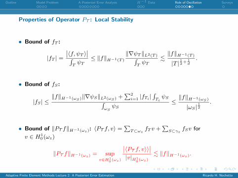
Properties of Operator PT : Local Stability

• Bound of fT :

|fT | =∣∣〈f, ψT 〉∣∣∫TψT

≤ ‖f‖H−1(T )

‖∇ψT ‖L2(T )∫TψT

.‖f‖H−1(T )

|T | 12 + 1d

.

• Bound of fS:

|fS | ≤‖f‖H−1(ωS)‖∇ψS‖L2(ωS) +

∑2i=1 |fTi |

∫TiψS∫

ωSψS

≤‖f‖H−1(ωS)

|ωS |12

.

• Bound of ‖PT f‖H−1(ωz): 〈PT f, v〉 =∑T⊂ωz

fT v +∑S⊂γz fSv for

v ∈ H10 (ωz)

‖PT f‖H−1(ωz) = supv∈H1

0 (ωz)

∣∣〈PT f, v〉〉∣∣|v|H1

0 (ωz)

. ‖f‖H−1(ωz).

Page 40: Adaptive Finite Element Methods Lecture 2: A Posteriori ... · Outline Model Problem A Posteriori Error Analysis H 1 Data Role of Oscillation Surveys A Priori Error Analysis If u2A

New Residual Estimator

• Local estimator: for all z ∈ N we have

E(U, ωz) = ‖PT f + ∆U‖2H−1(ωz)

≈∑T⊂ωz

h2z‖fT ‖2L2(T ) +

∑S⊂γz

hz‖j(U) + fS‖2L2(S).

• Jump residual: Modified jumps j(U) + fS appeared already in

I R.H. Nochetto, Pointwise a posteriori error estimates for elliptic problems onhighly graded meshes, Math. Comp., 64 (1995), 1-22.

I E. Bansch and P. Morin, and R.H. Nochetto, An adaptive Uzawa FEM for theStokes problem: Convergence without the inf-sup condition, SIAM J. Numer.Anal. 40 (2002), 1207–1229.

• Data oscillation: the term ‖f − PT f‖H−1(ωz) is not computable but it iscontrolled by the error ‖∇(u− U)‖L2(ωz).

Outline

Surveys

• R.H. Nochetto Adaptive FEM: Theory and Applications to GeometricPDE, Lipschitz Lectures, Haussdorff Center for Mathematics, University ofBonn (Germany), February 2009 (seewww.hausdorff-center.uni-bonn.de/event/2009/lipschitz-nochetto/).

• R.H. Nochetto, K.G. Siebert and A. Veeser, Theory of adaptivefinite element methods: an introduction, in Multiscale, Nonlinear andAdaptive Approximation, R. DeVore and A. Kunoth eds, Springer (2009),409-542.

• R.H. Nochetto and A. Veeser, Primer of adaptive finite elementmethods, in Multiscale and Adaptivity: Modeling, Numerics andApplications, CIME Lectures, eds R. Naldi and G. Russo, Springer, (2012),125–225.

adaptive finite element methods lecture 2: a posteriori ... · outline model problem a posteriori...

Documents