Adaptive Adaptive IndexingFelix Martin Schuhknecht1, Jens Dittrich2, Laurent Linden3

Saarland Informatics CampusSaarland University, Germany

1 felix.schuhknecht@infosys.uni-saarland.de2 jens.dittrich@infosys.uni-saarland.de

3 laurent.linden@gmx.net

Abstract—In nature, many species became extinct as theycould not adapt quickly enough to their environment. They weresimply not fit enough to adapt to more and more challengingcircumstances. Similar things happen when algorithms are toostatic to cope with particular challenges of their “environment”,be it the workload, the machine, or the user requirements.In this regard, in this paper we explore the well-researchedand fascinating family of adaptive indexing algorithms. Classicaladaptive indexes solely adapt the indexedness of the data to theworkload. However, we will learn that so far we have overlookeda second higher level of adaptivity, namely the one of the indexingalgorithm itself. We will coin this second level of adaptivitymeta-adaptivity.

Based on a careful experimental analysis, we will develop anadaptive index, which realizes meta-adaptivity by (1) generalizingthe way reorganization is performed, (2) reacting to the evolvingindexedness and varying reorganization effort, and (3) defusingskewed distributions in the input data. As we will demonstrate,this allows us to emulate the characteristics of a large setof specialized adaptive indexing algorithms. In an extensiveexperimental study we will show that our meta-adaptive indexis extremely fit in a variety of environments and outperforms alarge amount of specialized adaptive indexes under various queryaccess patterns and key distributions.

I. INTRODUCTION

An overwhelming amount of adaptive indexing algorithmsexists today. In our recent studies [1], [2], we analyzed 8 pa-pers including 18 different techniques on this type of indexing.The reason for the necessity of such a large number ofmethods is that adaptivity, while offering many nice properties,introduces a surprising amount of unpleasant problems [1],[2] as well. For instance, as the investigation of these worksshowed, adaptive indexing must deal with high variance, slowconvergence speed, weak robustness against different queryworkloads and data distributions, and the trade-off betweenindividual and accumulated query response time.

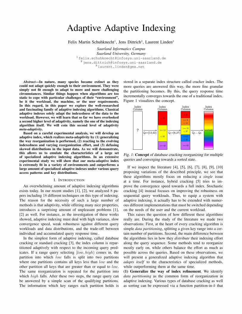
In the simplest form of adaptive indexing, called databasecracking or standard cracking [3], the index column is repar-titioned adaptively with respect to the incoming query pred-icates. If a range query selecting [low, high) comes in, thepartition into which low falls is split into two partitionswhere one partitions contains all keys less than low and theother partition all keys that are greater than or equal to low.The same reorganization is repeated for the partition intowhich high falls. After these two steps, the range query canbe answered by a simple scan of the qualifying partitions.The information which key ranges each partition holds is

stored in a separate index structure called cracker index. Themore queries are answered this way, the more fine granularthe partitioning becomes. By this, the query response timeincrementally converges towards the one of a traditional index.Figure 1 visualizes the concept.

?

Index Column

< 13

>= 13

< 42

>= 42

Index Column

Q0=[13,42)

Index Column

sortedQ2 Qn...Q1=[6,27)

< 6

>= 6< 13

>= 13< 27

>=27< 42

>= 42

Index Column

Fig. 1: Concept of database cracking reorganizing for multiplequeries and converging towards a sorted state.

If we inspect the literature [4], [5], [6], [7], [8], [9], [10]proposing variations of the described principle, we see thatthese algorithms mostly focus on reducing a single issueat a time. For instance, hybrid cracking [5] tries to im-prove the convergence speed towards a full index. Stochasticcracking [4] instead focuses on improving the robustness onsequential query workloads. Thus, to equip a system withadaptive indexing, it actually has to be extended with numer-ous different implementations that must be switched dependingon the needs of the user and the current workload.

This raises the question of how different these algorithmsreally are. During the study of the literature we made twoobservations: First, at the heart of every cracking algorithm issimple data partitioning, splitting a given key range into a cer-tain number of partitions. Second, the main difference betweenthe algorithms lies in how they distribute their indexing effortalong the query sequence. Some methods tend to reorganizemostly early on, while others balance the effort as much aspossible across the queries. Based on these observations, wewill present a generalized adaptive indexing algorithm thatadapts itself to the characteristics of specialized methods,while outperforming them at the same time.(1) Generalize the way of index refinement. We identifydata partitioning as the common form of reorganization inadaptive indexing. Various types of database cracking as wellas sorting can be expressed via a function partition-in-k that

produces k disjoint partitions. For instance, we can emulatestandard cracking (respectively crack-in-two) using k = 2,while sorting on 64-bit keys can be expressed using the fan-out k = 264. Consequently, partition-in-k will be the solecomponent of reorganization in our algorithm, realized usingboth in-place and out-of-place versions of highly efficient radixpartitioning techniques.(2) Adapt the reorganization effort by adjusting the parti-tioning fan-out k with respect to the size of the partition towork on. Classical approaches keep their reorganization effortstatic during their lifetime. For instance, crack-in-two splits itsinput always into two parts, independent of the partition sizeand the state of the index. However, the reorganization effortshould be carefully adapted to the input to refine the index asmuch as possible in an individual step without deteriorating thequery response time. To achieve this, we perform the followingstrategy: with a decrease in size of the input partition that hasto be refined, we increase the fan-out k of partition-in-k. Thus,we exploit the decrease in reorganization effort and reorganizemore fine-granular to speed up the convergence while ensuringfast response times. Consequently, if a partition reaches asufficiently small size, we “finish” it via sorting, also enablinginteresting orders on the data.(3) Identify and defuse skewed key distributions and adjustthe reorganization mechanism accordingly to counter them.By default, radix partitioning creates balanced partitions onlyif the key distribution is uniform. While uniformity is oftenpresent, it is careless to rely on it. Thus, we introduce amechanism that is able to defuse the problems caused bythe presence of skew in the very first query already. Weachieve two things: First, we are able to detect skew in theinput without overhead. Second, in the presence of skew, werecursively split partitions that are way larger than the averageto enforce a balanced processing of subsequent queries.

Following these three simple concepts, we are able toemulate a large set of specialized adaptive indexing algorithms.Via seven configuration parameters, our general algorithm canbe specialized to focus on properties such as convergencespeed, variance reduction, or the resistance towards skew, andthus it can emulate and possibly replace a large number ofspecialized indexes. We will generate method signatures tovisualize the quality of our emulation. Apart from applyingmanual configurations, we will use simulated annealing tooptimize the parameter set towards the minimal accumulatedquery response time for a given workload. Let us now see howwe can realize such a meta-adaptive algorithm.

II. GENERALIZING INDEX REFINEMENT

Simple data partitioning is at the core of any adaptive in-dexing algorithm. The applied fan-out of the partitioning pro-cess dictates the characteristics of the method by influencingconvergence speed, variance, and distribution of the indexingeffort. Thus, an algorithm that is able to set the fan-out of thepartitioning procedure freely is able to adapt to the behavior ofvarious adaptive indexing algorithms. Consequently, we willsolely use a partition-in-k step to perform the reorganization.

Apart from the used partitioning fan-out, the actual imple-mentation of partition-in-k plays an important role. Classicalapproaches mostly rely on comparison-based methods, asthey partition the keys with respect to the incoming querypredicates. We decided to use a radix based partitioningalgorithm as this type of reorganization method offers a higherpartitioning throughput than comparison-based methods [11].Of course, in contrast to comparison based methods, radixbased partitioning does not generate partitions with respectto the given predicates, and thus, filtering the generatedpartitions for qualifying entries is required. Still, consideringthe performance advantage, this is a price worth paying.

Further, we have to distinguish between the very first query,which can utilize an out-of-place partitioning algorithm, andsubsequent queries, where the index column is reorganizedsolely in-place. In the former case, we can use a highlyoptimized out-of-place radix partitioning, that has shown itssuperior performance already in our study [12]. It enhancesthe partitioning process using software-managed buffers, non-temporal streaming stores, and an optimized micro-layout. Inthe latter case, we use an in-place radix partitioning algorithm,that swaps elements between partitions in a cuckoo-stylefashion [13], without the need of additional memory. Bothalgorithms together build the core of reorganization in ourmeta-adaptive index and will be presented in detail in the nextsection.

III. ADAPTING REORGANIZATION EFFORT

With a look at the previous section, it remains the questionof how to steer the amount of reorganization. When should weinvest how much into partitioning? To approach this question,we will run a set of experiments to investigate the impactof varying fan-outs on the partitioning process in differentsituations. We have to distinguish between the very firstquery, which can exploit out-of-place partitioning, and theremaining ones, which reorganize in-place. Further, we haveto distinguish between different input partition sizes, as theyhighly influence the required cost of reorganization. Let usstart by looking solely on the first query.

A. Data Partitioning in the Very First Query

For the very first query, we analyze the runtime of the out-of-place partitioning of 100 million entries of 8B key and 8BrowID. The used machine is a mid-range server that we alsouse in the experimental evaluation later on (see Section VIII-Afor a detailed description). Thus, in total, around 1.5GB ofdata must be moved. The keys are picked in a uniformand random fashion from the entire unsigned 64-bit integerrange. We reorganize for a single range query [low, high),where the low predicate splits the key range into partitionsof size 1/3 and 2/3 of the data size. The high predicatesplits the partition of size 2/3 subsequently into two equalsized partitions. To reorganize for this query we consider twooptions: The classical way (as employed by standard cracking)is to partition the data out-of-place into two partitions withrespect to low and then to perform in-place crack-in-two onthe upper partition with respect to high. The created middle

0

0.5

1

1.5

2

2.5

3

3.5

4

4.54 8

16

32

64

128

256

512

1024

2048

4096

8192

16384

32768

Runtim

e in [s]

Partitioning Fanout

Out-of-place radix partitioningOut-of-place crack-in-two + In-place crack-in-two

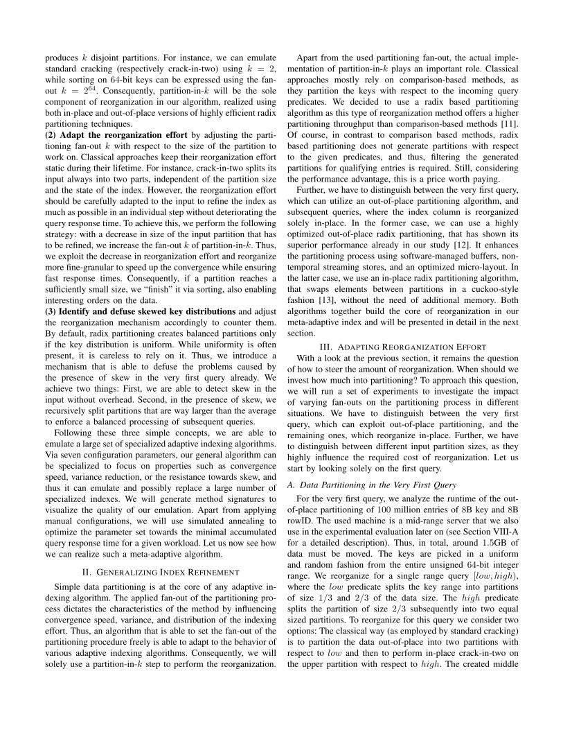
(a) Reorganization for the very first query. Standard crackingperforms an out-of-place crack-in-two step with respect to predi-cate low and an in-place crack-in-two step with respect to high.In comparison, we show out-of-place radix partitioning as presentedin [12] under a varying fan-out of 4 to 32,768.

0

5

10

15

20

25

30

35

4 32 512 4 32 512 4 32 512 4 32 512

32KB (L1) 256KB (L2) 2MB (Page) 10MB (L3)

Ru

ntim

e in

[m

s]

Partitioning Fanout

Input data size

2 x In-place crack-in-two2 x In-place radix partitioning

(b) Reorganization for a subsequent query. We test the partition inputsizes 32KB (L1 cache), 256KB (L2 cache), 2MB (HugePage), and 10MB(L3 cache). For in-place radix partitioning, we show fan-outs of 4, 32, and512 as representatives.

Fig. 2: Comparison of reorganization options for a range query selecting [low, high). We have to distinguish between the veryfirst query (Figure 2(a)), where the keys are copied from the base table into the index column, and subsequent queries (Figure 2(b)),that reorganize in-place. We test the strategy applied by standard cracking and compare it with radix partitioning.

partition answers the query. As an alternative, since we haveto copy the entire column anyway, we can ignore the querypredicates and instead directly partition the data out-of-placeusing our highly optimized radix based method [12] with acustom fan-out. Although this form of reorganization requiresadditional filtering to answer the query, it is a valid alternativeas the partitions to filter are small for reasonable fan-outs.

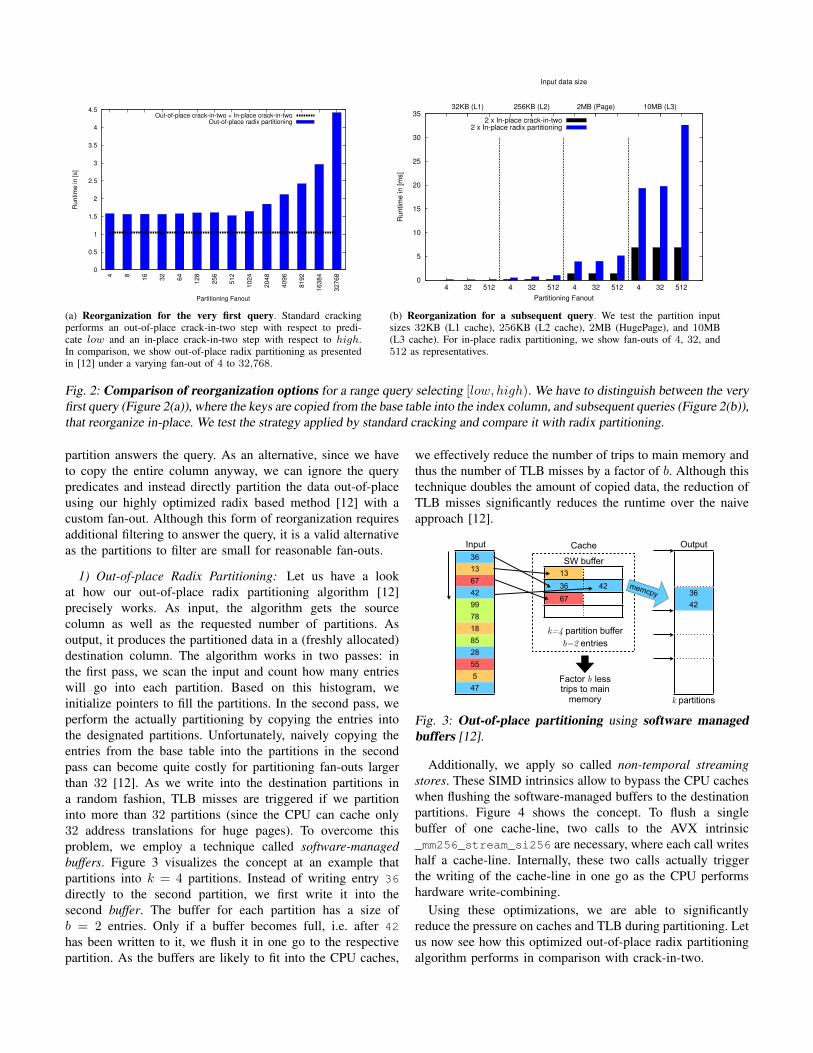
1) Out-of-place Radix Partitioning: Let us have a lookat how our out-of-place radix partitioning algorithm [12]precisely works. As input, the algorithm gets the sourcecolumn as well as the requested number of partitions. Asoutput, it produces the partitioned data in a (freshly allocated)destination column. The algorithm works in two passes: inthe first pass, we scan the input and count how many entrieswill go into each partition. Based on this histogram, weinitialize pointers to fill the partitions. In the second pass, weperform the actually partitioning by copying the entries intothe designated partitions. Unfortunately, naively copying theentries from the base table into the partitions in the secondpass can become quite costly for partitioning fan-outs largerthan 32 [12]. As we write into the destination partitions ina random fashion, TLB misses are triggered if we partitioninto more than 32 partitions (since the CPU can cache only32 address translations for huge pages). To overcome thisproblem, we employ a technique called software-managedbuffers. Figure 3 visualizes the concept at an example thatpartitions into k = 4 partitions. Instead of writing entry 36

directly to the second partition, we first write it into thesecond buffer. The buffer for each partition has a size ofb = 2 entries. Only if a buffer becomes full, i.e. after 42

has been written to it, we flush it in one go to the respectivepartition. As the buffers are likely to fit into the CPU caches,

we effectively reduce the number of trips to main memory andthus the number of TLB misses by a factor of b. Although thistechnique doubles the amount of copied data, the reduction ofTLB misses significantly reduces the runtime over the naiveapproach [12].

On the Surprising Difficulty of Simple Things:the Case of Radix Partitioning

Felix Martin Schuhknecht Pankaj Khanchandani Jens DittrichInformation Systems Group, Saarland University, infosys.uni-saarland.de

Original

0

1

2

3

4

5

1 10 100 1000

Radix

part

itionin

g tim

e [s]

Number of cache-lines per partition buffer

Numberof

Partitions

25

26

27

28

29

210

211

212

213

214

0

1

2

3

4

5

1 10 100 1000

Radix

part

itionin

g tim

e [s]

Number of cache-lines per partition buffer

Numberof

Partitions

25

26

27

28

29

210

211

212

213

214

0

1

2

3

4

5

1 10 100 1000

Radix

part

itionin

g tim

e [s]

Number of cache-lines per partition buffer

Numberof

Partitions

25

26

27

28

29

210

211

212

213

214

0

1

2

3

4

5

32 64 128 256 512 1024 2048 4096 8192 16384

Ra

dix

pa

rtiti

on

ing

tim

e [

s]

Number of partitions

Original (4KB)Original (2MB)

SW Buffers + Streaming store (4KB)SW Buffers + Streaming store (2MB)

SW

BUFFERS

STREAMING

STORES

PREFETCHING

MICRO

ROW

PAGE

SIZE

0

0.75

1.5

2.25

Number of partitions16384819240962048102451225612864R

educ

tion

of ru

ntim

eov

er o

rigin

al v

ersi

on [s

]

64

512

4KB: L1 dTLB

L2 TLB

32

-

2MB: L1 dTLB

L2 TLB

TLB Characteristics

361367429978188528555

47

Input Output

3642

1336 4267

k=4 partition bufferb=2 entries

k partitions

Cache

Factor b lesstrips to main

memory

memcpy

3642

Output

1336 4267

k partitions

_mm256_stream_si256

Cache

Cacheline36 42

Hardwarewrite-combine buffer

flush

Bypass cacheswhen writing output

Input Output

13 prefetch3667 prefetch

k partitions

Cache

prefetch

fill slot i ➞ prefetch slot i+1

SUMMARY

0

0.5

1

1.5

2

2.5

3

3.5

4

32 64 128 256 512 1024 2048 4096 8192 16384Number of partitions

Par

titio

ning

tim

e [s

]

SW Buffers

SW Buffers + Streaming

Original (prefetched)

SW Buffers + Streaming Stores

Original

SW Buffers + Streaming Stores + Micro Row Layout

E1 E2 E3 E4 E5 E6 E7 Fillstate Destination

Cacheline (64B)

8B 8B 8B 8B 8B 8B 8B 8BStore working

variables in last slot

Minimize number of accessed cachelines

361367429978188528555

47

_mm256_stream_si256

SW buffer

SW buffer

SW buffer

k=4 partition bufferb=2 entries

k=4 partition bufferb=2 entries

Fig. 3: Out-of-place partitioning using software managedbuffers [12].

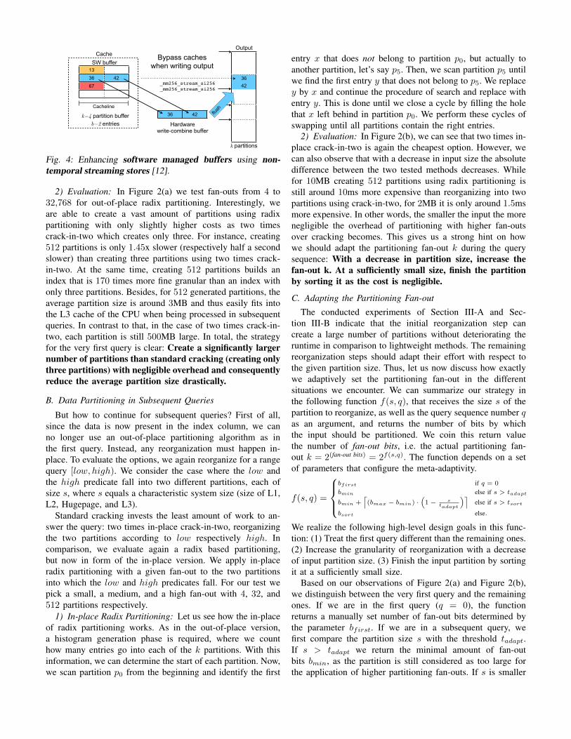
Additionally, we apply so called non-temporal streamingstores. These SIMD intrinsics allow to bypass the CPU cacheswhen flushing the software-managed buffers to the destinationpartitions. Figure 4 shows the concept. To flush a singlebuffer of one cache-line, two calls to the AVX intrinsic_mm256_stream_si256 are necessary, where each call writeshalf a cache-line. Internally, these two calls actually triggerthe writing of the cache-line in one go as the CPU performshardware write-combining.

Using these optimizations, we are able to significantlyreduce the pressure on caches and TLB during partitioning. Letus now see how this optimized out-of-place radix partitioningalgorithm performs in comparison with crack-in-two.

On the Surprising Difficulty of Simple Things:the Case of Radix Partitioning

Felix Martin Schuhknecht Pankaj Khanchandani Jens DittrichInformation Systems Group, Saarland University, infosys.uni-saarland.de

Original

0

1

2

3

4

5

1 10 100 1000

Radix

part

itionin

g tim

e [s]

Number of cache-lines per partition buffer

Numberof

Partitions

25

26

27

28

29

210

211

212

213

214

0

1

2

3

4

5

1 10 100 1000

Radix

part

itionin

g tim

e [s]

Number of cache-lines per partition buffer

Numberof

Partitions

25

26

27

28

29

210

211

212

213

214

0

1

2

3

4

5

1 10 100 1000

Radix

part

itionin

g tim

e [s]

Number of cache-lines per partition buffer

Numberof

Partitions

25

26

27

28

29

210

211

212

213

214

0

1

2

3

4

5

32 64 128 256 512 1024 2048 4096 8192 16384

Radix

part

itionin

g tim

e [s]

Number of partitions

Original (4KB)Original (2MB)

SW Buffers + Streaming store (4KB)SW Buffers + Streaming store (2MB)

SW

BUFFERS

STREAMING

STORES

PREFETCHING

MICRO

ROW

PAGE

SIZE

0

0.75

1.5

2.25

Number of partitions16384819240962048102451225612864Red

uctio

n of

runt

ime

over

orig

inal

ver

sion

[s]

64

512

4KB: L1 dTLB

L2 TLB

32

-

2MB: L1 dTLB

L2 TLB

TLB Characteristics

361367429978188528555

47

Input Output

3642

1336 4267

k=4 partition bufferb=2 entries

k partitions

Cache

Factor b lesstrips to main

memory

memcpy

3642

Output

1336 4267

k partitions

_mm256_stream_si256

Cache

Cacheline36 42

Hardwarewrite-combine buffer

flush

Bypass cacheswhen writing output

Input Output

13 prefetch3667 prefetch

k partitions

Cache

prefetch

fill slot i ➞ prefetch slot i+1

SUMMARY

0

0.5

1

1.5

2

2.5

3

3.5

4

32 64 128 256 512 1024 2048 4096 8192 16384Number of partitions

Par

titio

ning

tim

e [s

]

SW Buffers

SW Buffers + Streaming

Original (prefetched)

SW Buffers + Streaming Stores

Original

SW Buffers + Streaming Stores + Micro Row Layout

E1 E2 E3 E4 E5 E6 E7 Fillstate Destination

Cacheline (64B)

8B 8B 8B 8B 8B 8B 8B 8BStore working

variables in last slot

Minimize number of accessed cachelines

361367429978188528555

47

_mm256_stream_si256

SW buffer

SW buffer

SW buffer

k=4 partition bufferb=2 entries

k=4 partition bufferb=2 entries

Fig. 4: Enhancing software managed buffers using non-temporal streaming stores [12].

2) Evaluation: In Figure 2(a) we test fan-outs from 4 to32,768 for out-of-place radix partitioning. Interestingly, weare able to create a vast amount of partitions using radixpartitioning with only slightly higher costs as two timescrack-in-two which creates only three. For instance, creating512 partitions is only 1.45x slower (respectively half a secondslower) than creating three partitions using two times crack-in-two. At the same time, creating 512 partitions builds anindex that is 170 times more fine granular than an index withonly three partitions. Besides, for 512 generated partitions, theaverage partition size is around 3MB and thus easily fits intothe L3 cache of the CPU when being processed in subsequentqueries. In contrast to that, in the case of two times crack-in-two, each partition is still 500MB large. In total, the strategyfor the very first query is clear: Create a significantly largernumber of partitions than standard cracking (creating onlythree partitions) with negligible overhead and consequentlyreduce the average partition size drastically.

B. Data Partitioning in Subsequent Queries

But how to continue for subsequent queries? First of all,since the data is now present in the index column, we canno longer use an out-of-place partitioning algorithm as inthe first query. Instead, any reorganization must happen in-place. To evaluate the options, we again reorganize for a rangequery [low, high). We consider the case where the low andthe high predicate fall into two different partitions, each ofsize s, where s equals a characteristic system size (size of L1,L2, Hugepage, and L3).

Standard cracking invests the least amount of work to an-swer the query: two times in-place crack-in-two, reorganizingthe two partitions according to low respectively high. Incomparison, we evaluate again a radix based partitioning,but now in form of the in-place version. We apply in-placeradix partitioning with a given fan-out to the two partitionsinto which the low and high predicates fall. For our test wepick a small, a medium, and a high fan-out with 4, 32, and512 partitions respectively.

1) In-place Radix Partitioning: Let us see how the in-placeof radix partitioning works. As in the out-of-place version,a histogram generation phase is required, where we counthow many entries go into each of the k partitions. With thisinformation, we can determine the start of each partition. Now,we scan partition p0 from the beginning and identify the first

entry x that does not belong to partition p0, but actually toanother partition, let’s say p5. Then, we scan partition p5 untilwe find the first entry y that does not belong to p5. We replacey by x and continue the procedure of search and replace withentry y. This is done until we close a cycle by filling the holethat x left behind in partition p0. We perform these cycles ofswapping until all partitions contain the right entries.

2) Evaluation: In Figure 2(b), we can see that two times in-place crack-in-two is again the cheapest option. However, wecan also observe that with a decrease in input size the absolutedifference between the two tested methods decreases. Whilefor 10MB creating 512 partitions using radix partitioning isstill around 10ms more expensive than reorganizing into twopartitions using crack-in-two, for 2MB it is only around 1.5msmore expensive. In other words, the smaller the input the morenegligible the overhead of partitioning with higher fan-outsover cracking becomes. This gives us a strong hint on howwe should adapt the partitioning fan-out k during the querysequence: With a decrease in partition size, increase thefan-out k. At a sufficiently small size, finish the partitionby sorting it as the cost is negligible.

C. Adapting the Partitioning Fan-out

The conducted experiments of Section III-A and Sec-tion III-B indicate that the initial reorganization step cancreate a large number of partitions without deteriorating theruntime in comparison to lightweight methods. The remainingreorganization steps should adapt their effort with respect tothe given partition size. Thus, let us now discuss how exactlywe adaptively set the partitioning fan-out in the differentsituations we encounter. We can summarize our strategy inthe following function f(s, q), that receives the size s of thepartition to reorganize, as well as the query sequence number qas an argument, and returns the number of bits by whichthe input should be partitioned. We coin this return valuethe number of fan-out bits, i.e. the actual partitioning fan-out k = 2(fan-out bits) = 2f(s,q). The function depends on a setof parameters that configure the meta-adaptivity.

f(s, q) =

bfirst if q = 0

bmin else if s > tadapt

bmin +⌈(bmax − bmin) ·

(1 − s

tadapt

)⌉else if s > tsort

bsort else.

We realize the following high-level design goals in this func-tion: (1) Treat the first query different than the remaining ones.(2) Increase the granularity of reorganization with a decreaseof input partition size. (3) Finish the input partition by sortingit at a sufficiently small size.

Based on our observations of Figure 2(a) and Figure 2(b),we distinguish between the very first query and the remainingones. If we are in the first query (q = 0), the functionreturns a manually set number of fan-out bits determined bythe parameter bfirst. If we are in a subsequent query, wefirst compare the partition size s with the threshold tadapt.If s > tadapt we return the minimal amount of fan-outbits bmin, as the partition is still considered as too large forthe application of higher partitioning fan-outs. If s is smaller

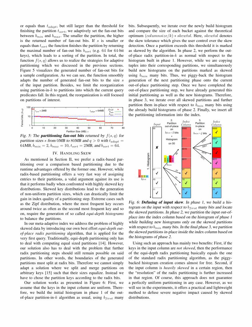
or equals than tadapt, but still larger than the threshold forfinishing the partition tsort, we adaptively set the fan-out bitsbetween bmin and bmax. The smaller the partition, the higheris the returned number of fan-out bits. If s is smaller orequals than tsort the function finishes the partition by returningthe maximal number of fan-out bits bsort (e.g. 64 for 64-bitkeys), which leads to a sorting of the partition. In total, thefunction f(s, q) allows us to realize the strategies for adaptivepartitioning which we discussed in the previous sections.Figure 5 visualizes the generated number of fan-out bits fora sample configuration. As we can see, the function smoothlyadapts the number of generated fan-out bits to the size sof the input partition. Besides, we limit the reorganizationusing partition-in-k to partitions into which the current querypredicates fall. In this regard, the reorganization is still focusedon partitions of interest.

1

10

100

0 10 20 30 40 50 60 70 80

Fanout bits:

f(s,

q)

Partition Size (MB): s

tadapt = 64MBtsort = 2MBf(s,q)bminbmax

Fig. 5: The partitioning fan-out bits returned by f(s, q) forpartition sizes s from 0MB to 80MB and q > 0 with tadapt =64MB, bmin = 2, bmax = 10, tsort = 2MB, and bsort = 64.

IV. HANDLING SKEW

As mentioned in Section II, we prefer a radix-based par-titioning over a comparison based partitioning due to theruntime advantages offered by the former one. However, whileradix-based partitioning offers a very fast way of assigningentries to their partitions, a valid argument against its use isthat it performs badly when confronted with highly skewed keydistributions. Skewed key distributions lead to the generationof non-uniform partition sizes, which can drastically limit thegain in index quality of a partitioning step. Extreme cases suchas the Zipf distribution, where the most frequent key occursaround twice as often as the second most frequent key and soon, require the generation of so called equi-depth histogramsto balance the partitions.

In our meta-adaptive index we address the problem of highlyskewed data by introducing our own best effort equi-depth out-of-place radix partitioning algorithm, that is applied for thevery first query. Traditionally, equi-depth partitioning only hasto deal with computing equal sized partitions [14]. However,our solution also has to deal with the problem that furtherradix partitioning steps should still remain possible on saidpartitions. In other words, the boundaries of the generatedpartitions must split at radix bits. Therefore we cannot simplyadapt a solution where we split and merge partitions onarbitrary keys [15] such that their sizes equalize. Instead wehave to chose the partition keys according to the radix bits.

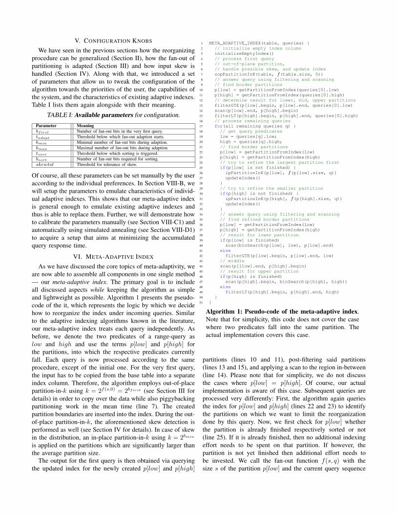
Our solution works as presented in Figure 6: First, weassume that the keys in the input column are uniform. There-fore, we build the initial histogram in phase 1 of the out-of-place partition-in-k algorithm as usual, using bfirst many

bits. Subsequently, we iterate over the newly build histogramand compare the size of each bucket against the theoreticaloptimum (columnsize/k) ∗ skewtol. Here, skewtol denotesthe skew tolerance which gives the user control over the skewdetection. Once a partition exceeds this threshold it is markedas skewed by the algorithm. In phase 2, we perform the out-of-place radix partition-in-k as normal with respect to thehistogram built in phase 1. However, while we are copyingtuples into their corresponding partitions, we simultaneouslybuild new histograms on the partitions marked as skewedusing bmin many bits. Thus, we piggy-back the histogramgeneration of the next partitioning phase onto the currentout-of-place partitioning step. Once we have completed theout-of-place partitioning step, we have already generated thisinitial partitioning as well as the new histograms. Therefore,in phase 3, we iterate over all skewed partitions and furtherpartition them in-place with respect to bmin many bits usingthe already build histograms of phase 2. Finally, we insert allthe partitioning information into the index.

✘

✓

✓

✓

Input

1. H

isto

gram

IndexColumn

✓

✓

✓

2. Partition

out-of-place on

bfirst=2 bits+

Histogram on 00

00

01

10

11

0000

01

10

11

0001

0010

0011

IndexColumn

✓

✓

✓

✓

✓

✓

✓

0000

01

10

11

0001

0010

0011

3. Partitionin-place

on bmin=4 bits

00

01

10

11

0000

0001

00100011

bfirst

bmin

00 01 10 11

0000

0001

0010

0011

Fig. 6: Defusing of input skew. In phase 1, we build a his-togram on the input with respect to bfirst many bits and locatethe skewed partitions. In phase 2, we partition the input out-of-place into the index column based on the histogram of phase 1while building new histograms only on the skewed partitionswith respect to bmin many bits. In the final phase 3, we partitionthe skewed partitions in-place inside the index column based onthe histograms of phase 2.

Using such an approach has mainly two benefits: First, if thekeys in the input column are not skewed, then the performanceof the equi-depth radix partitioning basically equals the oneof the standard radix partitioning algorithm, as the piggy-backed histogram creation comes almost for free. Second, ifthe input column is heavily skewed in a certain region, thenthe “resolution” of the radix partitioning is further increasedin that region. Of course, this approach does not guaranteea perfectly uniform partitioning in any case. However, as wewill see in the experiments, it offers a practical and lightweightmethod to defuse severe negative impact caused by skeweddistributions.

V. CONFIGURATION KNOBS

We have seen in the previous sections how the reorganizingprocedure can be generalized (Section II), how the fan-out ofpartitioning is adapted (Section III) and how input skew ishandled (Section IV). Along with that, we introduced a setof parameters that allow us to tweak the configuration of thealgorithm towards the priorities of the user, the capabilities ofthe system, and the characteristics of existing adaptive indexes.Table I lists them again alongside with their meaning.

TABLE I: Available parameters for configuration.

Parameter Meaningbfirst Number of fan-out bits in the very first query.tadapt Threshold below which fan-out adaption starts.bmin Minimal number of fan-out bits during adaption.bmax Maximal number of fan-out bits during adaption.tsort Threshold below which sorting is triggered.bsort Number of fan-out bits required for sorting.skewtol Threshold for tolerance of skew.

Of course, all these parameters can be set manually by the useraccording to the individual preferences. In Section VIII-B, wewill setup the parameters to emulate characteristics of individ-ual adaptive indexes. This shows that our meta-adaptive indexis general enough to emulate existing adaptive indexes andthus is able to replace them. Further, we will demonstrate howto calibrate the parameters manually (see Section VIII-C1) andautomatically using simulated annealing (see Section VIII-D1)to acquire a setup that aims at minimizing the accumulatedquery response time.

VI. META-ADAPTIVE INDEX

As we have discussed the core topics of meta-adaptivity, weare now able to assemble all components in one single method— our meta-adaptive index. The primary goal is to includeall discussed aspects while keeping the algorithm as simpleand lightweight as possible. Algorithm 1 presents the pseudo-code of the it, which represents the logic by which we decidehow to reorganize the index under incoming queries. Similarto the adaptive indexing algorithms known in the literature,our meta-adaptive index treats each query independently. Asbefore, we denote the two predicates of a range-query aslow and high and use the terms p[low] and p[high] forthe partitions, into which the respective predicates currentlyfall. Each query is now processed according to the sameprocedure, except of the initial one. For the very first query,the input has to be copied from the base table into a separateindex column. Therefore, the algorithm employs out-of-placepartition-in-k using k = 2f(s,0) = 2bfirst (see Section III fordetails) in order to copy over the data while also piggybackingpartitioning work in the mean time (line 7). The createdpartition boundaries are inserted into the index. During the out-of-place partition-in-k, the aforementioned skew detection isperformed as well (see Section IV for details). In case of skewin the distribution, an in-place partition-in-k using k = 2bmin

is applied on the partitions which are significantly larger thanthe average partition size.

The output for the first query is then obtained via queryingthe updated index for the newly created p[low] and p[high]

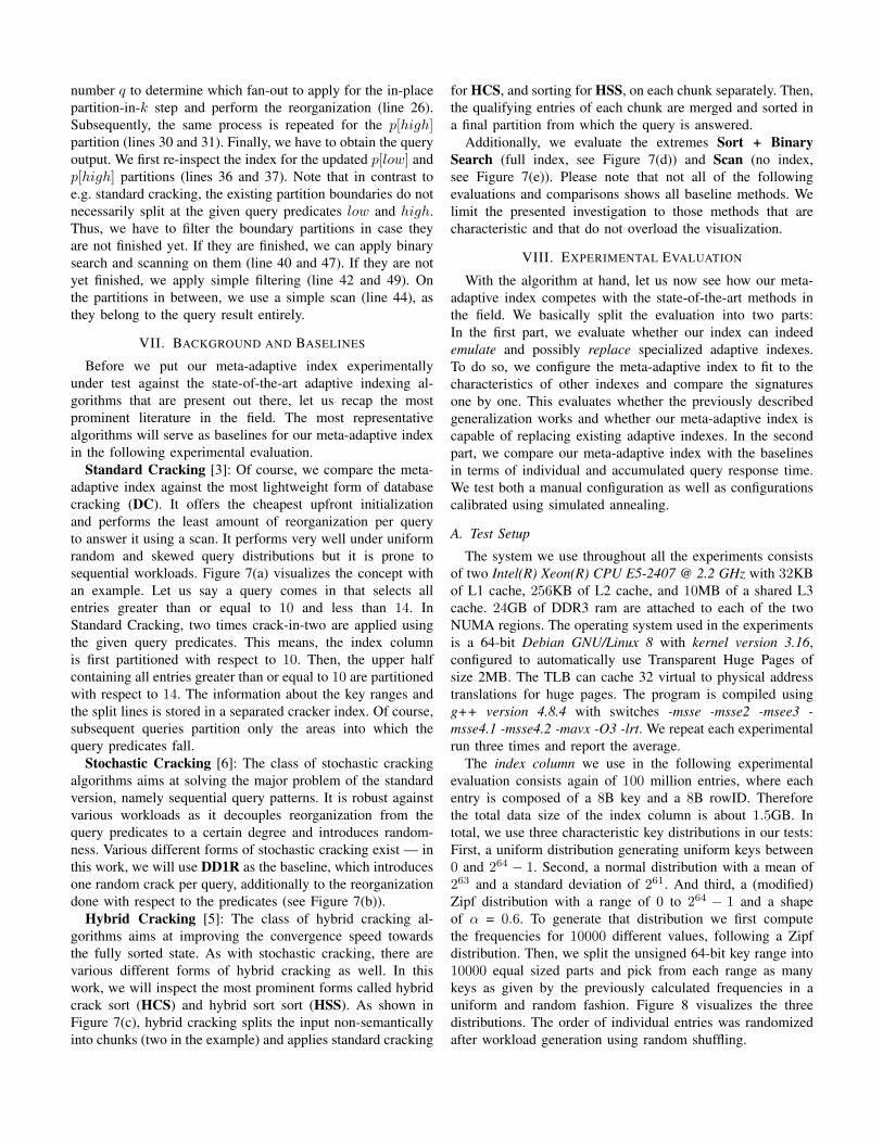
1 META_ADAPTIVE_INDEX(table, queries) {2 // initialize empty index column3 initializeEmptyIndex()4 // process first query5 // out-of-place partition,6 // handle possible skew, and update index7 oopPartitionInK(table, f(table.size, 0))8 // answer query using filtering and scanning9 // find border partitions

10 p[low] = getPartitionFromIndex(queries[0].low)11 p[high] = getPartitionFromIndex(queries[0].high)12 // determine result for lower, mid, upper partitions13 filterGTE(p[low].begin, p[low].end, queries[0].low)14 scan(p[low].end, p[high].begin)15 filterLT(p[high].begin, p[high].end, queries[0].high)16 // process remaining queries17 for(all remaining queries q) {18 // get query predicates19 low = queries[q].low;20 high = queries[q].high;21 // find border partitions22 p[low] = getPartitionFromIndex(low)23 p[high] = getPartitionFromIndex(high)24 // try to refine the largest partition first25 if(p[low] is not finished) {26 ipPartitionInK(p[low], f(p[low].size, q))27 updateIndex()28 }29 // try to refine the smaller partition30 if(p[high] is not finished) {31 ipPartitionInK(p[high], f(p[high].size, q))32 updateIndex()33 }34 // answer query using filtering and scanning35 // find refined border partitions36 p[low] = getPartitionFromIndex(low)37 p[high] = getPartitionFromIndex(high)38 // result for lower partition39 if(p[low] is finished)40 scan(binSearch(p[low], low), p[low].end)41 else42 filterGTE(p[low].begin, p[low].end, low)43 // middle44 scan(p[llow].end, p[high].begin)45 // result for upper partition46 if(p[high] is finished)47 scan(p[high].begin, binSearch(p[high], high))48 else49 filterLT(p[high].begin, p[high].end, high)50 }51 }

Algorithm 1: Pseudo-code of the meta-adaptive index.Note that for simplicity, this code does not cover the casewhere two predicates fall into the same partition. Theactual implementation covers this case.

partitions (lines 10 and 11), post-filtering said partitions(lines 13 and 15), and applying a scan to the region in-between(line 14). Please note that for simplicity, we do not discussthe cases where p[low] = p[high]. Of course, our actualimplementation is aware of this case. Subsequent queries areprocessed very differently: First, the algorithm again queriesthe index for p[low] and p[high] (lines 22 and 23) to identifythe partitions on which we want to limit the reorganizationdone by this query. Now, we first check for p[low] whetherthe partition is already finished respectively sorted or not(line 25). If it is already finished, then no additional indexingeffort needs to be spent on that partition. If however, thepartition is not yet finished then additional effort needs tobe invested. We call the fan-out function f(s, q) with thesize s of the partition p[low] and the current query sequence

number q to determine which fan-out to apply for the in-placepartition-in-k step and perform the reorganization (line 26).Subsequently, the same process is repeated for the p[high]partition (lines 30 and 31). Finally, we have to obtain the queryoutput. We first re-inspect the index for the updated p[low] andp[high] partitions (lines 36 and 37). Note that in contrast toe.g. standard cracking, the existing partition boundaries do notnecessarily split at the given query predicates low and high.Thus, we have to filter the boundary partitions in case theyare not finished yet. If they are finished, we can apply binarysearch and scanning on them (line 40 and 47). If they are notyet finished, we apply simple filtering (line 42 and 49). Onthe partitions in between, we use a simple scan (line 44), asthey belong to the query result entirely.

VII. BACKGROUND AND BASELINES

Before we put our meta-adaptive index experimentallyunder test against the state-of-the-art adaptive indexing al-gorithms that are present out there, let us recap the mostprominent literature in the field. The most representativealgorithms will serve as baselines for our meta-adaptive indexin the following experimental evaluation.

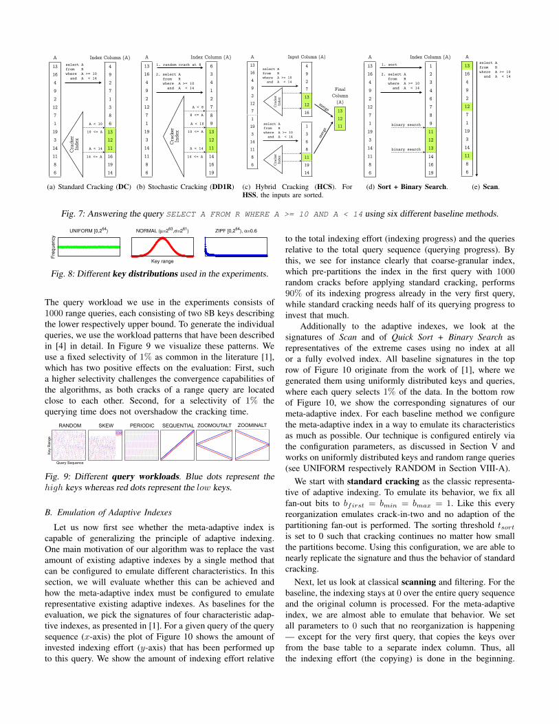
Standard Cracking [3]: Of course, we compare the meta-adaptive index against the most lightweight form of databasecracking (DC). It offers the cheapest upfront initializationand performs the least amount of reorganization per queryto answer it using a scan. It performs very well under uniformrandom and skewed query distributions but it is prone tosequential workloads. Figure 7(a) visualizes the concept withan example. Let us say a query comes in that selects allentries greater than or equal to 10 and less than 14. InStandard Cracking, two times crack-in-two are applied usingthe given query predicates. This means, the index columnis first partitioned with respect to 10. Then, the upper halfcontaining all entries greater than or equal to 10 are partitionedwith respect to 14. The information about the key ranges andthe split lines is stored in a separated cracker index. Of course,subsequent queries partition only the areas into which thequery predicates fall.

Stochastic Cracking [6]: The class of stochastic crackingalgorithms aims at solving the major problem of the standardversion, namely sequential query patterns. It is robust againstvarious workloads as it decouples reorganization from thequery predicates to a certain degree and introduces random-ness. Various different forms of stochastic cracking exist — inthis work, we will use DD1R as the baseline, which introducesone random crack per query, additionally to the reorganizationdone with respect to the predicates (see Figure 7(b)).

Hybrid Cracking [5]: The class of hybrid cracking al-gorithms aims at improving the convergence speed towardsthe fully sorted state. As with stochastic cracking, there arevarious different forms of hybrid cracking as well. In thiswork, we will inspect the most prominent forms called hybridcrack sort (HCS) and hybrid sort sort (HSS). As shown inFigure 7(c), hybrid cracking splits the input non-semanticallyinto chunks (two in the example) and applies standard cracking

for HCS, and sorting for HSS, on each chunk separately. Then,the qualifying entries of each chunk are merged and sorted ina final partition from which the query is answered.

Additionally, we evaluate the extremes Sort + BinarySearch (full index, see Figure 7(d)) and Scan (no index,see Figure 7(e)). Please note that not all of the followingevaluations and comparisons shows all baseline methods. Welimit the presented investigation to those methods that arecharacteristic and that do not overload the visualization.

VIII. EXPERIMENTAL EVALUATION

With the algorithm at hand, let us now see how our meta-adaptive index competes with the state-of-the-art methods inthe field. We basically split the evaluation into two parts:In the first part, we evaluate whether our index can indeedemulate and possibly replace specialized adaptive indexes.To do so, we configure the meta-adaptive index to fit to thecharacteristics of other indexes and compare the signaturesone by one. This evaluates whether the previously describedgeneralization works and whether our meta-adaptive index iscapable of replacing existing adaptive indexes. In the secondpart, we compare our meta-adaptive index with the baselinesin terms of individual and accumulated query response time.We test both a manual configuration as well as configurationscalibrated using simulated annealing.

A. Test Setup

The system we use throughout all the experiments consistsof two Intel(R) Xeon(R) CPU E5-2407 @ 2.2 GHz with 32KBof L1 cache, 256KB of L2 cache, and 10MB of a shared L3cache. 24GB of DDR3 ram are attached to each of the twoNUMA regions. The operating system used in the experimentsis a 64-bit Debian GNU/Linux 8 with kernel version 3.16,configured to automatically use Transparent Huge Pages ofsize 2MB. The TLB can cache 32 virtual to physical addresstranslations for huge pages. The program is compiled usingg++ version 4.8.4 with switches -msse -msse2 -msee3 -msse4.1 -msse4.2 -mavx -O3 -lrt. We repeat each experimentalrun three times and report the average.

The index column we use in the following experimentalevaluation consists again of 100 million entries, where eachentry is composed of a 8B key and a 8B rowID. Thereforethe total data size of the index column is about 1.5GB. Intotal, we use three characteristic key distributions in our tests:First, a uniform distribution generating uniform keys between0 and 264 − 1. Second, a normal distribution with a mean of263 and a standard deviation of 261. And third, a (modified)Zipf distribution with a range of 0 to 264 − 1 and a shapeof α = 0.6. To generate that distribution we first computethe frequencies for 10000 different values, following a Zipfdistribution. Then, we split the unsigned 64-bit key range into10000 equal sized parts and pick from each range as manykeys as given by the previously calculated frequencies in auniform and random fashion. Figure 8 visualizes the threedistributions. The order of individual entries was randomizedafter workload generation using random shuffling.

13164921271193141186

A49271386131211161914

Index Column (A)

10 <= A

14 <= A

A < 10

Crac

ker

Inde

x

select A from R where A >= 10 and A < 14

A < 14

(a) Standard Cracking (DC)

13164921271193141186

A Index Column (A)

2. select A from R where A >= 10 and A < 14

Crac

ker

Inde

x

1. random crack at 8 63412789131211141619

10 <= A

14 <= A

A < 10

A < 14

A < 8

8 <= A

(b) Stochastic Cracking (DD1R)

13164921271193141186

A Input Column (A)

select A from R where A >= 10 and A < 14

select A from R where A >= 10 and A < 14

Crac

ker

Inde

xCr

acke

rIn

dex

131211

merge

4927131216

1368111914

merg

e

Final Column

(A)

(c) Hybrid Cracking (HCS). ForHSS, the inputs are sorted.

13164921271193141186

A Index Column (A)

2. select A from R where A >= 10 and A < 14

1. sort 12346789111213141619

binary search

binary search

(d) Sort + Binary Search.

13164921271193141186

Aselect A from R where A >= 10 and A < 14

(e) Scan.

Fig. 7: Answering the query SELECT A FROM R WHERE A >= 10 AND A < 14 using six different baseline methods.

Fre

qu

en

cy

UNIFORM [0,264

)

Key range

NORMAL (µ=263

,σ=261

) ZIPF [0,264

), α=0.6

Fig. 8: Different key distributions used in the experiments.

The query workload we use in the experiments consists of1000 range queries, each consisting of two 8B keys describingthe lower respectively upper bound. To generate the individualqueries, we use the workload patterns that have been describedin [4] in detail. In Figure 9 we visualize these patterns. Weuse a fixed selectivity of 1% as common in the literature [1],which has two positive effects on the evaluation: First, sucha higher selectivity challenges the convergence capabilities ofthe algorithms, as both cracks of a range query are locatedclose to each other. Second, for a selectivity of 1% thequerying time does not overshadow the cracking time.

RANDOM SKEW PERIODIC

Key

Range

SEQUENTIAL

Query Sequence

ZOOMOUTALT ZOOMINALT

RANDOM SKEW PERIODIC

Key

Range

SEQUENTIAL

Query Sequence

ZOOMOUTALT ZOOMINALT

RANDOM SKEW PERIODIC

Key

Range

SEQUENTIAL

Query Sequence

ZOOMOUTALT ZOOMINALT

RANDOM SKEW PERIODIC

Key

Range

SEQUENTIAL

Query Sequence

ZOOMOUTALT ZOOMINALT

RANDOM SKEW PERIODIC

Key

Range

SEQUENTIAL

Query Sequence

ZOOMOUTALT ZOOMINALT

RANDOM SKEW PERIODIC

Ke

y R

an

ge

SEQUENTIAL

Query Sequence

ZOOMOUTALT ZOOMINALTZOOMOUTALT ZOOMINALTSEQUENTIALPERIODICSKEWRANDOM

Query Sequence

Key

Ran

ge

Fig. 9: Different query workloads. Blue dots represent thehigh keys whereas red dots represent the low keys.

B. Emulation of Adaptive Indexes

Let us now first see whether the meta-adaptive index iscapable of generalizing the principle of adaptive indexing.One main motivation of our algorithm was to replace the vastamount of existing adaptive indexes by a single method thatcan be configured to emulate different characteristics. In thissection, we will evaluate whether this can be achieved andhow the meta-adaptive index must be configured to emulaterepresentative existing adaptive indexes. As baselines for theevaluation, we pick the signatures of four characteristic adap-tive indexes, as presented in [1]. For a given query of the querysequence (x-axis) the plot of Figure 10 shows the amount ofinvested indexing effort (y-axis) that has been performed upto this query. We show the amount of indexing effort relative

to the total indexing effort (indexing progress) and the queriesrelative to the total query sequence (querying progress). Bythis, we see for instance clearly that coarse-granular index,which pre-partitions the index in the first query with 1000random cracks before applying standard cracking, performs90% of its indexing progress already in the very first query,while standard cracking needs half of its querying progress toinvest that much.

Additionally to the adaptive indexes, we look at thesignatures of Scan and of Quick Sort + Binary Search asrepresentatives of the extreme cases using no index at allor a fully evolved index. All baseline signatures in the toprow of Figure 10 originate from the work of [1], where wegenerated them using uniformly distributed keys and queries,where each query selects 1% of the data. In the bottom rowof Figure 10, we show the corresponding signatures of ourmeta-adaptive index. For each baseline method we configurethe meta-adaptive index in a way to emulate its characteristicsas much as possible. Our technique is configured entirely viathe configuration parameters, as discussed in Section V andworks on uniformly distributed keys and random range queries(see UNIFORM respectively RANDOM in Section VIII-A).

We start with standard cracking as the classic representa-tive of adaptive indexing. To emulate its behavior, we fix allfan-out bits to bfirst = bmin = bmax = 1. Like this everyreorganization emulates crack-in-two and no adaption of thepartitioning fan-out is performed. The sorting threshold tsortis set to 0 such that cracking continues no matter how smallthe partitions become. Using this configuration, we are able tonearly replicate the signature and thus the behavior of standardcracking.

Next, let us look at classical scanning and filtering. For thebaseline, the indexing stays at 0 over the entire query sequenceand the original column is processed. For the meta-adaptiveindex, we are almost able to emulate that behavior. We setall parameters to 0 such that no reorganization is happening— except for the very first query, that copies the keys overfrom the base table to a separate index column. Thus, allthe indexing effort (the copying) is done in the beginning.

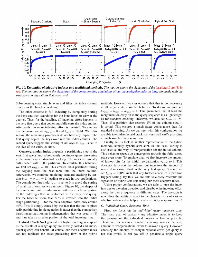
Fig. 10: Emulation of adaptive indexes and traditional methods. The top row shows the signatures of the baselines from [1] inred. The bottom row shows the signatures of the corresponding emulations of our meta-adaptive index in blue, alongside with theparameter configurations that were used.

Subsequent queries simply scan and filter the index columnexactly as the baseline is doing it.

The other extreme is full indexing by completely sortingthe keys and then searching for the boundaries to answer thequeries. Thus, for the baseline, all indexing effort happens inthe very first query that copies and fully sorts the index entries.Afterwards, no more indexing effort is invested. To emulatethis behavior, we set bfirst = 0 and tsort = 100M. With thissetting, the remaining parameters do not have any impact. Thefirst query copies the keys over into the index column. Thesecond query triggers the sorting of all keys as tsort is set tothe size of the entire column.

Coarse-granular index prepends a partitioning step to thevery first query and subsequently continues query answeringin the same way as standard cracking. The index is basicallybulk-loaded with 1000 partitions. To emulate this behavior,we first set bfirst = 10. This creates 1024 partitions duringthe copying from the base table into the index column.Afterwards, we continue emulating standard cracking by set-ting bmin = bmax = 1, leading to crack-in-two applications.The completion threshold tsort is set to 0 to avoid the sortingof small partitions. As we can see in Figure 10, the shapes ofthe curves are quite similar — in both cases, a large portionof the indexing effort is performed in the very first query.For the baseline, more than 80% is invested into the initialrange partitioning — for the meta-adaptive index, only around40%. This is simply caused by the fact that the out-of-placeradix partitioning implementation is faster than the comparisonbased range-partitioning implementation that was used in [1]and thus takes a smaller portion of the total indexing time.

Hybrid Crack Sort generates a higher convergence speedas the results of a range query are directly sorted and subse-quent queries can benefit. Of course, our meta-adaptive indexcan not replicate the exact processing flow of the hybrid

methods. However, we can observe that this is not necessaryat all to generate a similar behavior. To do so, we first setbfirst = bmin = bmax = 1. This guarantees that at least thereorganization early on in the query sequence is as lightweightas for standard cracking. However, we also set tsort = 1M.Thus, if a partition size reaches 1% of the column size, itis sorted. This ensures a much faster convergence than forstandard cracking. As we can see, with this configuration weare able to emulate hybrid crack sort very well while providinga much simpler processing flow.

Finally, let us look at another representative of the hybridmethods, namely hybrid sort sort. In this case, sorting isalso used as the way of reorganization for the initial column.This behavior speeds up convergence towards the fully sortedstate even more. To emulate that, we first increase the amountof fan-out bits for the initial reorganization bfirst to 8. Thisdoes not fully sort the column, but increases the amount ofinvested indexing effort in the very first query. Second, weset tsort = 100M such that any further access of a partitiontriggers sorting. By this, we are able to closely resemble thesignature of hybrid sort sort using our meta-adaptive index.

Using proper configurations, we are able to tune the indexinto one or the other direction and distribute the indexing effortalong the query sequence in different ways. The question isnow: does the ability to adapt to the characteristics of variousadaptive indexes also help in terms of query response times?

C. Individual Query Response TimeFirst, we focus on the individual query response time.

The main goal of basically any adaptive index is to keepthe pressure on the individual queries as low as possible.Therefore, for instance standard cracking invests the leastamount of reorganizational work to answer a query. However,choosing the amount of reorganizational effort per query isnot that trivial. It can pay off to penalize a single query

Meta-adaptive Index (Manually configured)DC DD1R HCS

1

10

100

1000

10000

1 10 100 1000

Sing

le Q

uery

Res

pons

e Ti

me

[ms]

Query Sequence

Sort + Binary Search

(a) U(min = 0,max = 264 − 1)

1

10

100

1000

10000

1 10 100 1000

Sin

gle

Query

Response T

ime [m

s]

Query Sequence

(b) N (µ = 263, σ = 261)

1

10

100

1000

10000

1 10 100 1000

Sin

gle

Query

Response T

ime [m

s]

Query Sequence

(c) Z(min = 0,max = 264 − 1, α = 0.6)

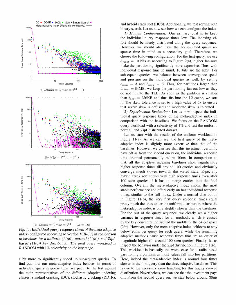
Fig. 11: Individual query response times of the meta-adaptiveindex (configured according to Section VIII-C1) in comparisonto baselines for a uniform (11(a)), normal (11(b)), and Zipf-based (11(c)) key distribution. The used query workload isRANDOM with 1% selectivity on the key range.

a bit more to significantly speed up subsequent queries. Tofind out how our meta-adaptive index behaves in terms ofindividual query response time, we put it to the test againstthe main representatives of the different adaptive indexingclasses: standard cracking (DC), stochastic cracking (DD1R),

and hybrid crack sort (HCS). Additionally, we test sorting withbinary search. Let us now see how we can configure the index.

1) Manual Configuration: Our primary goal is to keepthe individual query response times low. The indexing ef-fort should be nicely distributed along the query sequence.However, we should also have the accumulated query re-sponse time in mind as a secondary goal. Therefore, wechoose the following configuration: For the first query, we usebfirst = 10 bits as according to Figure 2(a), higher fan-outsmake the partitioning significantly more expensive. Thus, withindividual response time in mind, 10 bits are the limit. Forsubsequent queries, we balance between convergence speedand pressure on the individual queries as well, by settingbmin = 3 and bmax = 6. Thus, for partitions larger thantadapt = 64MB, we keep the partitioning fan-out low as theydo not fit into the TLB. As soon as the partition is smallerthan tsort = 256KB and thus fits into the L2 cache, we sortit. The skew tolerance is set to a high value of 5x to ensurethat severe skew is defused and moderate skew is tolerated.

2) Experimental Evaluation: Let us now inspect the indi-vidual query response times of the meta-adaptive index incomparison with the baselines. We focus on the RANDOMquery workload with a selectivity of 1% and test the uniform,normal, and Zipf distributed dataset.

Let us start with the results of the uniform workload inFigure 11(a). As we can see, the first query of the meta-adaptive index is slightly more expensive than that of thebaselines. However, we can see that this investment certainlypays off as from the second query on, the individual responsetime dropped permanently below 10ms. In comparison tothat, all the adaptive indexing baselines show significantlyhigher response times till around 100 queries and obviouslyconverge much slower towards the sorted state. Especiallyhybrid crack sort shows very high response times even after100 seen queries if it has to merge entries into the finalcolumn. Overall, the meta-adaptive index shows the moststable performance and offers early on fast individual responsetimes, similar to the full index. Under a normal distributionin Figure 11(b), the very first query response times equalpretty much the ones under the uniform distribution, where themeta-adaptive index is only slightly slower than the baselines.For the rest of the query sequence, we clearly see a highervariance in response times for all methods, which is causedby the key concentration around the middle of the 64-bit space(263). However, only the meta-adaptive index achieves to staybelow 20ms per query for each query, while the remainingadaptive methods cause response times that are an order ofmagnitude higher till around 100 seen queries. Finally, let usinspect the behavior under the Zipf distribution in Figure 11(c).This workload is basically the worst case for a radix basedpartitioning algorithm, as most values fall into few partitions.Here, indeed the meta-adaptive index is around four timesslower in the first query than the three adaptive baselines. Thisis due to the necessary skew handling for this highly skeweddistribution. Nevertheless, we can see that the investment paysoff: From the second query on, we stay below around 30ms

per query, while the remaining methods show the spread wehave seen previously already. Overall, we can see how wellthe meta-adaptive index behaves in terms of individual queryresponse time under these extreme key distributions. It is ableto outperform the three main representatives of the majoradaptive indexing classes. Let us now see how it behaves interms of accumulated query response times.

D. Accumulated Query Response Time

To test the performance with respect to accumulated queryresponse time, we use again the manual configuration ofSection VIII-C1. The evaluation of the individual responsetime indicated already that this configuration is also a veryvalid choice in terms of accumulated time. Nevertheless, wealso want to evaluate how well an automatically generatedconfiguration can perform. Thus, we use simulated annealingto come up with a configuration, that tries to optimize theparameters with respect to accumulated response time. Thus,let us first discuss how simulated annealing works conceptuallyand how it can be applied in our case.

1) Automatic Configuration: As the parameters to configuredepend on each other, we use simulated annealing [16] to con-firm that a particular set of parameters indeed results in shortaccumulated query response times. We implement simulatedannealing as described in [17]. It is a well known technique forapproximating the global optimum of a function via stochasticprobing. The general idea is to start with an initial configu-ration and a hot temperature. The temperature is decreasedevery few steps. While the temperature continues to decrease,the configuration is varied in every step. The magnitude ofchange in the configuration depends on (1) the temperaturetemp, (2) a random number r ∈ [0, 1), and (3) manually setminimum and maximum values for the parameters to vary.After a certain temperature threshold is reached the algorithmstops. The final configuration is considered to be a reasonableapproximation of the global minimum.

For the initial configuration we choose the parameters basedon the manual configuration of our previous experiments. Thetemperature temp is initialized to 1.0, and is reduced viadivision (by a constant α) of 2.0 in this case. The numberof steps performed per temperature is set to 12, which istwice the number of parameters to optimize (bsort is fixedto 64 and thus not considered). The parameters to changeare chosen based on a rotation. The probability pAccept ofaccepting a ”worse” configuration is set to e−(dQRT/temp),where dQRT represents the change in accumulated queryresponse times. The stopping criterion is set so that the finalconfiguration is obtained if either temp reaches approximately0.0 or the configuration does not change between 20 tem-perature changes. As a quality function we simply use theaccumulated query response time of the meta-adaptive indexunder the given configuration. The time to reach the finalconfiguration is essentially dominated by the execution of theworkload using the individual configurations. For example, forthe uniform random workload, reaching the final configurationtook 28 minutes. For each of the three key distributions, we

perform an individual simulated annealing run to obtain aspecialized configuration. In each case, we use the randomquery pattern as a representative workload. Table II presentsthe three obtained configurations.

TABLE II: Configuration to minimize accumulated query re-sponse time as determined by simulated annealing.

Parameter Uniform Normal Zipfbfirst 12 bits 10 bits 5 bitsbmin 2 bits 1 bit 3 bitsbmax 5 bits 5 bits 5 bitstadapt 218MB 102MB 211MBtsort 354KB 32KB 32KBskewtol 4x 5x 5x

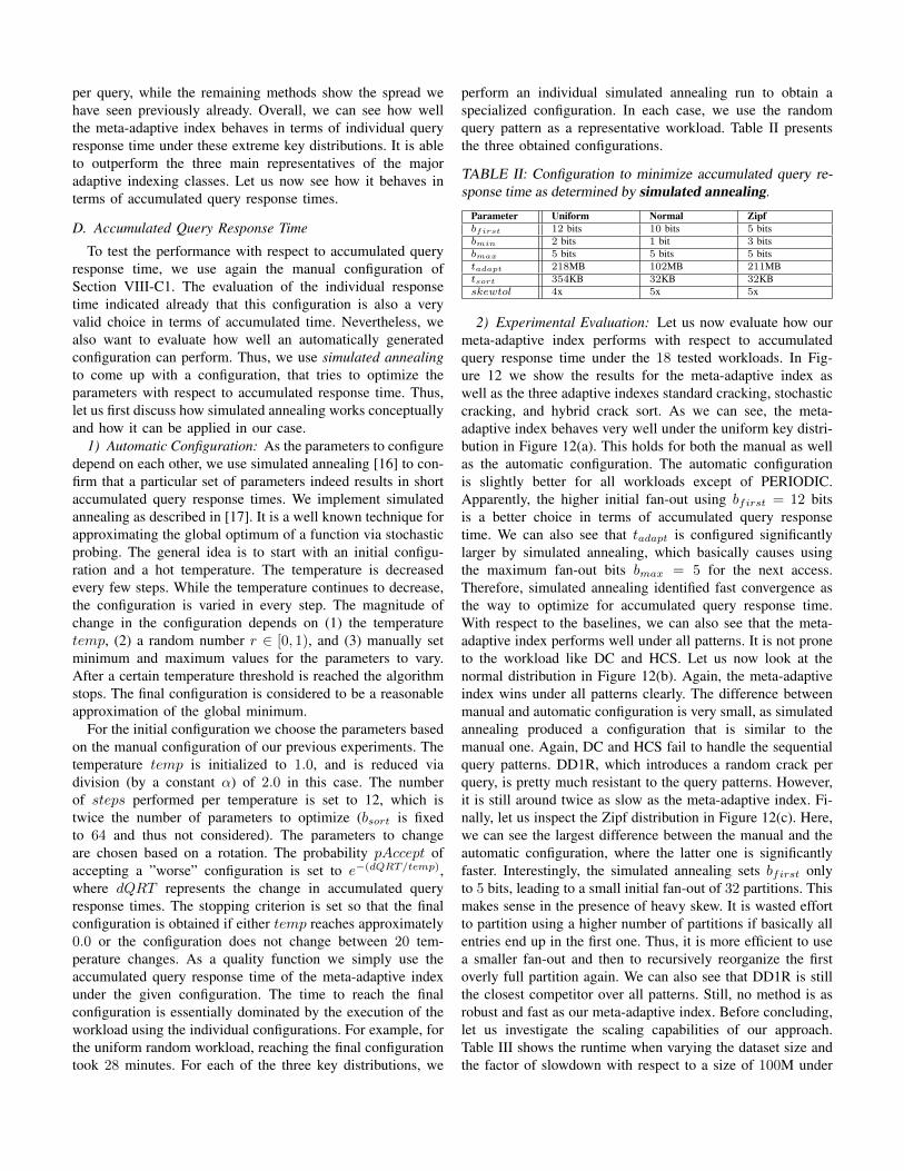
2) Experimental Evaluation: Let us now evaluate how ourmeta-adaptive index performs with respect to accumulatedquery response time under the 18 tested workloads. In Fig-ure 12 we show the results for the meta-adaptive index aswell as the three adaptive indexes standard cracking, stochasticcracking, and hybrid crack sort. As we can see, the meta-adaptive index behaves very well under the uniform key distri-bution in Figure 12(a). This holds for both the manual as wellas the automatic configuration. The automatic configurationis slightly better for all workloads except of PERIODIC.Apparently, the higher initial fan-out using bfirst = 12 bitsis a better choice in terms of accumulated query responsetime. We can also see that tadapt is configured significantlylarger by simulated annealing, which basically causes usingthe maximum fan-out bits bmax = 5 for the next access.Therefore, simulated annealing identified fast convergence asthe way to optimize for accumulated query response time.With respect to the baselines, we can also see that the meta-adaptive index performs well under all patterns. It is not proneto the workload like DC and HCS. Let us now look at thenormal distribution in Figure 12(b). Again, the meta-adaptiveindex wins under all patterns clearly. The difference betweenmanual and automatic configuration is very small, as simulatedannealing produced a configuration that is similar to themanual one. Again, DC and HCS fail to handle the sequentialquery patterns. DD1R, which introduces a random crack perquery, is pretty much resistant to the query patterns. However,it is still around twice as slow as the meta-adaptive index. Fi-nally, let us inspect the Zipf distribution in Figure 12(c). Here,we can see the largest difference between the manual and theautomatic configuration, where the latter one is significantlyfaster. Interestingly, the simulated annealing sets bfirst onlyto 5 bits, leading to a small initial fan-out of 32 partitions. Thismakes sense in the presence of heavy skew. It is wasted effortto partition using a higher number of partitions if basically allentries end up in the first one. Thus, it is more efficient to usea smaller fan-out and then to recursively reorganize the firstoverly full partition again. We can also see that DD1R is stillthe closest competitor over all patterns. Still, no method is asrobust and fast as our meta-adaptive index. Before concluding,let us investigate the scaling capabilities of our approach.Table III shows the runtime when varying the dataset size andthe factor of slowdown with respect to a size of 100M under

DC DD1R HCS

5

10

15

20

25

RA

ND

OM

SK

EW

ED

PE

RIO

DIC

SE

QU

EN

TIA

L

ZO

OM

OU

TA

LT

ZO

OM

INA

LT

Acc

um

. Q

uery

Resp

onse

Tim

e [s]

Query Workloads

DCDD1R

HCS

Madaptive Index (Manually configured)Madaptive Index (Simulated annealing configured)Meta-adaptive Index (Simulated annealing configured)

Meta-adaptive Index (Manually configured)

Query Workloads

(a) U(min = 0,max = 264 − 1)

5

10

15

20

25

RAND

OM

SKEW

ED

PERI

ODI

C

SEQ

UENT

IAL

ZOO

MO

UTAL

T

ZOO

MIN

ALT

Accu

m. Q

uery

Res

pons

e Ti

me

[s]

Query Workloads

Query Workloads

(b) N (µ = 263, σ = 261)

5

10

15

20

25

RA

ND

OM

SK

EW

ED

PE

RIO

DIC

SE

QU

EN

TIA

L

ZO

OM

OU

TA

LT

ZO

OM

INA

LT

Accum

. Q

uery

Response T

ime [s]

Query Workloads

(c) Z(min = 0,max = 264 − 1, α = 0.6)

Fig. 12: Accumulated query response times of the meta-adaptive index both manually configured (Section VIII-C1)as well automatically configured using simulated annealing(Section VIII-D1) under uniform (12(a)), normal (12(b)),and Zipf-based (12(c)) key distributions and different queryworkloads (see Section VIII-A).

the random uniform workload. As we can see, our approachscales linearly with respect to the datasize.

TABLE III: Scaling of the Meta-adaptive Index (manuallyconfigured) under uniform random workload.

Size 25M 50M 100M 200M 300M 400M 500M

Runtime 1.17s 2.39s 4.77s 9.63s 14.37s 19.82s 24.47sScaling 0.24x 0.50x 1x 2.01x 3.01x 4.15x 5.13x

IX. CONCLUSION

Our initial goal of the meta-adaptive index was to developa technique which can fulfill several of the core needs ofadaptive indexing at once. Firstly, we wanted to unify the largeamount of specialized adaptive indexes that aim at improvinga specific problem at a time in a single general method. Weachieved this by identifying the fact that partitioning is at thecore of any adaptive indexing algorithm. We proposed a meta-adaptive index that can emulate a large set of specialized in-dexes, which we were able to show by inspecting the indexingsignatures. Based on this, we secondly looked at how the meta-adaptive index compares with respect to the classical adaptiveindexing baselines and showed its superior performance under18 different workloads with an average speedup of around 2xover the best baseline. Thirdly, we looked at how to manuallyand automatically configure the meta-adaptive index. Usingsimulated annealing, we were able to push the performanceof the meta-adaptive index to the limits. Overall, the meta-adaptive index serves as a valid alternative for a large numberof specialized indexes and is able to improve in terms ofrobustness, runtime, and convergence speed over the state-of-the-art methods.

REFERENCES

[1] F. M. Schuhknecht, A. Jindal, and J. Dittrich, “The uncracked pieces indatabase cracking,” PVLDB, vol. 7, no. 2, pp. 97–108, 2013.

[2] Felix Martin Schuhknecht, Alekh Jindal and Jens Dittrich, “An experi-mental evaluation and analysis of database cracking,” VLDBJ, 2015.

[3] S. Idreos, M. L. Kersten, and S. Manegold, “Database cracking,” CIDR,pp. 68–78, 2007.

[4] F. Halim, S. Idreos, P. Karras, and R. H. C. Yap, “Stochastic databasecracking: Towards robust adaptive indexing in main-memory column-stores,” PVLDB, vol. 5, no. 6, pp. 502–513, 2012.

[5] S. Idreos, S. Manegold, H. Kuno, and G. Graefe, “Merging what’scracked, cracking what’s merged: Adaptive indexing in main-memorycolumn-stores,” PVLDB, vol. 4, no. 9, pp. 585–597, 2011.

[6] S. Idreos, M. Kersten, and S. Manegold, “Self-organizing tuple recon-struction in column-stores,” in SIGMOD 2009, pp. 297–308.

[7] H. Pirk, E. Petraki, S. Idreos, S. Manegold, and M. L. Kersten, “Databasecracking: fancy scan, not poor man’s sort!” in DaMoN, Snowbird, UT,USA, June 23, 2014, pp. 4:1–4:8.

[8] V. Alvarez, F. M. Schuhknecht, J. Dittrich, and S. Richter, “Mainmemory adaptive indexing for multi-core systems,” in DaMoN 2014,Snowbird, UT, USA, June 23, 2014, pp. 3:1–3:10.

[9] G. Graefe, F. Halim, S. Idreos et al., “Concurrency control for adaptiveindexing,” PVLDB, vol. 5, no. 7, pp. 656–667, 2012.

[10] Goetz Graefe, Felix Halim, Stratos Idreos et al, “Transactional supportfor adaptive indexing,” VLDBJ, vol. 23, no. 2, pp. 303–328, 2014.

[11] O. Polychroniou and K. A. Ross, “A comprehensive study of main-memory partitioning and its application to large-scale comparison- andradix-sort,” in SIGMOD 2014, pp. 755–766.

[12] F. M. Schuhknecht, P. Khanchandani, and J. Dittrich, “On the surprisingdifficulty of simple things: the case of radix partitioning,” PVLDB, vol. 8,no. 9, pp. 934–937, 2015.

[13] A. Maus, “Arl, a faster in-place, cache friendly sorting algorithm,” NorskInformatik konferranse NIK, vol. 2002, pp. 85–95, November 2002.

[14] Y. Ioannidis and V. Poosala, “Balancing histogram optimality andpracticality for query result size estimation,” in SIGMOD 1995, pp. 233–244.

[15] A. Aboulnaga and S. Chaudhuri, “Self-tuning histograms: Buildinghistograms without looking at data,” in SIGMOD 1999, pp. 181–192.

[16] A. Belloni, T. Liang, H. Narayanan, and A. Rakhlin, “Escaping the localminima via simulated annealing: Optimization of approximately convexfunctions,” in COLT 2015, pp. 240–265.

[17] R. Eglese, “Simulated annealing: A tool for operational research,”European Journal of Operational Research, vol. 46, no. 3, pp. 271 –281, 1990.