active contours without edges - image processing, ieee ...lvese/papers/ieeeip2001.pdf · chan and...

266 IEEE TRANSACTIONS ON IMAGE PROCESSING, VOL. 10, NO. 2, FEBRUARY 2001

Active Contours Without EdgesTony F. Chan, Member, IEEE,and Luminita A. Vese

Abstract—In this paper, we propose a new model for active con-tours to detect objects in a given image, based on techniques ofcurve evolution, Mumford–Shah functional for segmentation andlevel sets. Our model can detect objects whose boundaries are notnecessarily defined by gradient. We minimize an energy which canbe seen as a particular case of the minimal partition problem. Inthe level set formulation, the problem becomes a “mean-curvatureflow”-like evolving the active contour, which will stop on the de-sired boundary. However, the stopping term does not depend onthe gradient of the image, as in the classical active contour models,but is instead related to a particular segmentation of the image. Wewill give a numerical algorithm using finite differences. Finally, wewill present various experimental results and in particular someexamples for which the classical snakes methods based on the gra-dient are not applicable. Also, the initial curve can be anywhere inthe image, and interior contours are automatically detected.

Index Terms—Active contours, curvature, energy minimization,finite differences, level sets, partial differential equations, segmen-tation.

I. INTRODUCTION

T HE BASIC idea in active contour models or snakes is toevolve a curve, subject to constraints from a given image

, in order to detect objects in that image. For instance, startingwith a curve around the object to be detected, the curve movestoward its interior normal and has to stop on the boundary of theobject.

Let be a bounded open subset of, with its boundary.Let be a given image, and be aparameterized curve.

In the classical snakes and active contour models (see [9], [3],[13], [4]), an edge-detector is used, depending on the gradientof the image , to stop the evolving curve on the boundary ofthe desired object. We briefly recall these models next.

The snake model [9] is: , where

(1)

Here, , and are positive parameters. The first two termscontrol the smoothness of the contour (the internal energy),while the third term attracts the contour toward the object in

Manuscript received June 17, 1999; revised September 27, 2000. This workwas supported in part by ONR under Contract N00014-96-1-0277 and NSF Con-tract DMS-9626755. The associate editor coordinating the review of this man-uscript and approving it for publication was Prof. Robert J. Schalkoff.

The authors are with the Mathematics Department, University of Cali-fornia, Los Angeles, CA 90095-1555 USA (e-mail: [email protected];[email protected]).

Publisher Item Identifier S 1057-7149(01)00819-3.

the image (the external energy). Observe that, by minimizingthe energy (1), we are trying to locate the curve at the pointsof maxima , acting as an edge-detector, while keeping asmoothness in the curve (object boundary).

A general edge-detector can be defined by a positive and de-creasing function , depending on the gradient of the image,such that

For instance

where , a smoother version of , is the convo-lution of the image with the Gaussian

. The function is positive inhomogeneous regions, and zero at the edges.

In problems of curve evolution, the level set method and inparticular the motion by mean curvature of Osher and Sethian[19] have been used extensively, because it allows for cusps,corners, and automatic topological changes. Moreover, the dis-cretization of the problem is made on a fixed rectangular grid.The curve is represented implicitly via a Lipschitz function,by , and the evolution of the curve isgiven by the zero-level curve at timeof the function .Evolving the curve in normal direction with speed amountsto solve the differential equation [19]

where the set defines the initial contour.A particular case is the motion by mean curvature, whendiv is the curvature of the level-curve of

passing through . The equation becomes

div

A geometric active contour model based on the mean curva-ture motion is given by the following evolution equation [3]:

div

in

in

(2)

whereedge-function with ;is constant;initial level set function.

1057–7149/01$10.00 © 2001 IEEE

CHAN AND VESE: ACTIVE CONTOURS WITHOUT EDGES 267

Its zero level curve moves in the normal direction with speedand therefore stops on the desired

boundary, where vanishes. The constantis a correction termchosen so that the quantitydivremains always positive. This constant may be interpreted as aforce pushing the curve toward the object, when the curvaturebecomes null or negative. Also, is a constraint on the areainside the curve, increasing the propagation speed.

Two other active contour models based on level sets wereproposed in [13], again using the image gradient to stop thecurve. The first one is

in

where is a constant, and and are the maximum andminimum values of the magnitude of the image gradient

. Again, the speed of the evolving curve becomes zero on thepoints with highest gradients, and therefore the curve stops onthe desired boundary, defined by strong gradients. The secondmodel [13] is similar to the geometric model [3], with .Other related works are [14] and [15].

The geodesic model [4] is

(3)

This is a problem of geodesic computation in a Riemannianspace, according to a metric induced by the image. Solvingthe minimization problem (3) consists in finding the path ofminimal new length in that metric. A minimizer will be ob-tained when vanishes, i.e., when the curveis on the boundary of the object. The geodesic active contourmodel (3) from [4] also has a level set formulation

div

in

in

(4)

Because all these classical snakes and active contour modelsrely on the edge-function, depending on the image gradient

, to stop the curve evolution, these models can detect onlyobjects with edges defined by gradient. In practice, the dis-crete gradients are bounded and then the stopping functionis never zero on the edges, and the curve may pass throughthe boundary, especially for the models in [3], [13]–[15]. If theimage is very noisy, then the isotropic smoothing Gaussianhas to be strong, which will smooth the edges too. In this paper,we propose a different active contour model, without a stoppingedge-function, i.e. a model which is not based on the gradientof the image for the stopping process. The stopping term isbased on Mumford–Shah segmentation techniques [18]. In thisway, we obtain a model which can detect contours both with orwithout gradient, for instance objects with very smooth bound-aries or even with discontinuous boundaries (for a discussion on

different types of contours, we refer the reader to [8]). In addi-tion, our model has a level set formulation, interior contours areautomatically detected, and the initial curve can be anywhere inthe image.

The outline of the paper is as follows. In the next section weintroduce our model as an energy minimization and discuss therelationship with the Mumford–Shah functional for segmenta-tion. Also, we formulate the model in terms of level set functionsand compute the associated Euler–Lagrange equations. In Sec-tion III we present an iterative algorithm for solving the problemand its discretization. In Section IV we validate our model byvarious numerical results on synthetic and real images, showingthe advantages of our model described before, and we end thepaper by a brief concluding section.

Other related works are [29], [10], [26], and [24] on activecontours and segmentation, [28] and [11] on shape reconstruc-tion from unorganized points, and finally the recent works [20]and [21], where a probability based geodesic active regionmodel combined with classical gradient based active contourtechniques is proposed.

II. DESCRIPTION OF THEMODEL

Let us define the evolving curve in , as the boundary of anopen subset of (i.e. , and ). In what follows,inside denotes the region , andoutside denotes theregion .

Our method is the minimization of an energy based-segmen-tation. Let us first explain the basic idea of the model in a simplecase. Assume that the imageis formed by two regions of ap-proximatively piecewise-constant intensities, of distinct values

and . Assume further that the object to be detected is repre-sented by the region with the value. Let denote its boundaryby . Then we have inside the object [orinside( )],and outside the object [oroutside( )]. Now let usconsider the following “fitting” term:

where is any other variable curve, and the constants, ,depending on , are the averages of inside and respec-tively outside . In this simple case, it is obvious that , theboundary of the object, is the minimizer of the fitting term

This can be seen easily. For instance, if the curveis outsidethe object, then and . If the curve isinside the object, then but . If the curve

is both inside and outside the object, then and. Finally, the fitting energy is minimized if ,

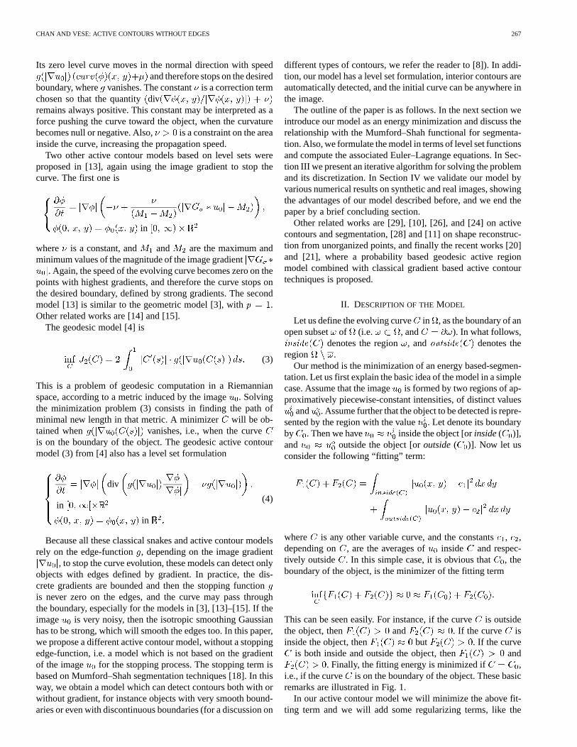
i.e., if the curve is on the boundary of the object. These basicremarks are illustrated in Fig. 1.

In our active contour model we will minimize the above fit-ting term and we will add some regularizing terms, like the


Fig. 1. Consider all possible cases in the position of the curve. The fitting termis minimized only in the case when the curve is on the boundary of the object.

length of the curve , and (or) the area of the region inside.Therefore, we introduce the energy functional , de-fined by

Length Area inside

where , , are fixed parameters. In almostall our numerical calculations (see further), we fixand .

Therefore, we consider the minimization problem:

Remark 1: In our model, the term Length could bere-written in a more general way asLength , with .If we consider the case of an arbitrary dimension (i.e.,

), then can have the following values: forall , or . For the last expression, we usethe isoperimetric inequality [7], which says in some sense thatLength is “comparable” with Areainside :

Area inside Length

where is a constant depending only on.

A. Relation with the Mumford–Shah Functional

The Mumford–Shah functional for segmentation is [18]

Length

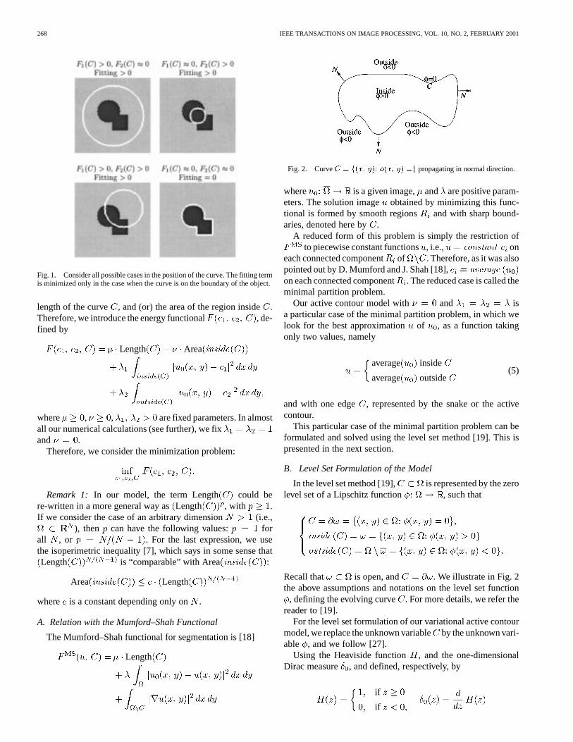
Fig. 2. CurveC = f(x; y): �(x; y) =g propagating in normal direction.

where is a given image, and are positive param-eters. The solution imageobtained by minimizing this func-tional is formed by smooth regions and with sharp bound-aries, denoted here by.

A reduced form of this problem is simply the restriction ofto piecewise constant functions, i.e., constant on

each connected componentof . Therefore, as it was alsopointed out by D. Mumford and J. Shah [18], average

on each connected component. The reduced case is called theminimal partition problem.

Our active contour model with and isa particular case of the minimal partition problem, in which welook for the best approximation of , as a function takingonly two values, namely

average inside

average outside(5)

and with one edge , represented by the snake or the activecontour.

This particular case of the minimal partition problem can beformulated and solved using the level set method [19]. This ispresented in the next section.

B. Level Set Formulation of the Model

In the level set method [19], is represented by the zerolevel set of a Lipschitz function , such that

inside

outside

Recall that is open, and . We illustrate in Fig. 2the above assumptions and notations on the level set function

, defining the evolving curve . For more details, we refer thereader to [19].

For the level set formulation of our variational active contourmodel, we replace the unknown variableby the unknown vari-able , and we follow [27].

Using the Heaviside function , and the one-dimensionalDirac measure , and defined, respectively, by

if

if


(in the sense of distributions), we express the terms in the energyin the following way (see also [7]):

Length

Area

and

Then, the energy can be written as

We note that, as defined in (5), solution of our modelas a particular case of the Mumford–Shah minimal partitionproblem, can simply be written using the level set formulationas

Keeping fixed and minimizing the energywith respect to the constants and , it is easy to expressthese constants function ofby

(6)

if (i.e. if the curve has a nonemptyinterior in ), and

(7)

if (i.e. if the curve has anonempty exterior in ). For the corresponding “degenerate”

cases, there are no constrains on the values ofand . Then,and are in fact given by

average in

average in

Remark 2: By the previous formulas, we can see that the en-ergy can be written only function of , which is the charac-teristic function of the set . Let us denote it by . Then wecan rewrite the energy in the new form

Therefore, we can consider the new minimization problem

a e (8)

among characteristic functions of sets with finite perimeter in. Here, a e means almost everywhere with respect to the

Lebesgue measure.We expect, of course, to have existence of minimizers of the

energy , due to several general results: our modelis a particular case of the minimal partition problem, for whichthe existence has been proved in [18] (assuming thatis con-tinuous on ), and also in [16] and [17], for more general data

. Also, the existence for the general Mumford–Shah segmen-tation problem has been proved in [5]. On the other hand, it canbe easily shown, by the lower-semicontinuity of the total varia-tion and classical arguments of calculus of vari-ations, that our minimization problem (8) has minimizers (thiscan be an alternative proof of the existence). In this paper, thelevel set function is used only to represent the curve and ithas many numerical advantages, but the problem could also beformulated and solved only in terms of characteristic functions.

In order to compute the associated Euler–Lagrange equationfor the unknown function , we consider slightly regularizedversions of the functions and , denoted here by and ,as . Let beany regularization of , and

. We will give further examples of such approximations. Letus denote by the associated regularized functional, definedby


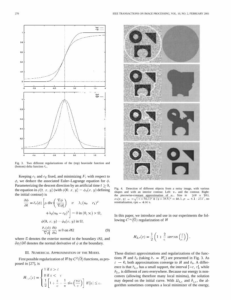
Fig. 3. Two different regularizations of the (top) heaviside function and(bottom) delta function� .

Keeping and fixed, and minimizing with respect to, we deduce the associated Euler–Lagrange equation for.

Parameterizing the descent direction by an artificial time ,the equation in (with definingthe initial contour) is

div

in

in

on (9)

where denotes the exterior normal to the boundary, anddenotes the normal derivative ofat the boundary.

III. N UMERICAL APPROXIMATION OF THEMODEL

First possible regularization of by functions, as pro-posed in [27], is

if

if

if

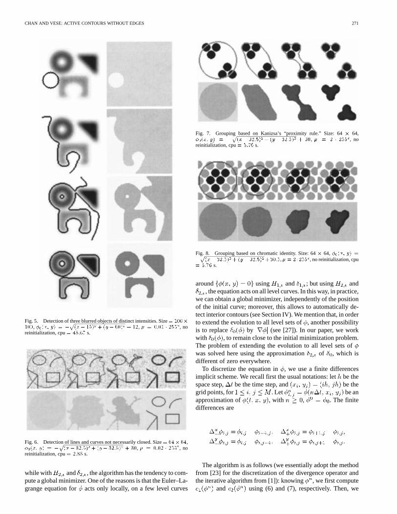
Fig. 4. Detection of different objects from a noisy image, with variousshapes and with an interior contour. Left:u and the contour. Right:the piecewise-constant approximation ofu . Size = 100 � 100,� (x; y) = � (x� 50:5) + (y � 50:5) + 48:5, � = 0:1 � 255 , noreinitialization, cpu= 4:60 s.

In this paper, we introduce and use in our experiments the fol-lowing regularization of

These distinct approximations and regularizations of the func-tions and (taking ) are presented in Fig. 3. As

, both approximations converge to and . A differ-ence is that has a small support, the interval , while

is different of zero everywhere. Because our energy is non-convex (allowing therefore many local minima), the solutionmay depend on the initial curve. With and , the al-gorithm sometimes computes a local minimizer of the energy,


Fig. 5. Detection of three blurred objects of distinct intensities. Size= 100�100, � (x; y) = � (x� 15) + (y � 60) + 12, � = 0:01 � 255 , noreinitialization, cpu= 48:67 s.

Fig. 6. Detection of lines and curves not necessarily closed. Size= 64� 64,� (x; y) = � (x� 32:5) + (y � 32:5) + 30, � = 0:02 � 255 , noreinitialization, cpu= 2:88 s.

while with and , the algorithm has the tendency to com-pute a global minimizer. One of the reasons is that the Euler–La-grange equation for acts only locally, on a few level curves

Fig. 7. Grouping based on Kanizsa’s “proximity rule.” Size: 64� 64,� (x; y) = � (x� 32:5) + (y � 32:5) + 30, � = 2 � 255 , noreinitialization, cpu= 5:76 s.

Fig. 8. Grouping based on chromatic identity. Size: 64� 64, � (x; y) =� (x� 32:5) + (y � 32:5) +30:5,� = 2 �255 , no reinitialization, cpu= 5:76 s.

around using and ; but using and, the equation acts on all level curves. In this way, in practice,

we can obtain a global minimizer, independently of the positionof the initial curve; moreover, this allows to automatically de-tect interior contours (see Section IV). We mention that, in orderto extend the evolution to all level sets of, another possibilityis to replace by (see [27]). In our paper, we workwith , to remain close to the initial minimization problem.The problem of extending the evolution to all level sets ofwas solved here using the approximation of , which isdifferent of zero everywhere.

To discretize the equation in, we use a finite differencesimplicit scheme. We recall first the usual notations: letbe thespace step, be the time step, and be thegrid points, for . Let be anapproximation of , with , . The finitedifferences are

The algorithm is as follows (we essentially adopt the methodfrom [23] for the discretization of the divergence operator andthe iterative algorithm from [1]): knowing , we first compute

and using (6) and (7), respectively. Then, we


Fig. 9. Object with smooth contour. Top: results using our model without edge-function. Bottom: results using the classical model (2) with edge-function.

compute by the following discretization and linearizationof (9) in

This linear system is solved by an iterative method, and for moredetails, werefer the reader to [1].

When working with level sets and Dirac delta functions, astandard procedure is to reinitialize to the signed distancefunction to its zero-level curve, as in [25] and [27]. This pre-vents the level set function to become too flat, or it can be seenas a rescaling and regularization. For our algorithm, the reini-tialization is optional. On the other hand, it should not be toostrong, because, as it was remarked by Fedkiw, it prevents in-terior contours from growing. Only for a few numerical resultswe have applied the reinitialization, solving the following evo-lution equation [25]:

sign(10)

where is our solution at time . Then the newwill be , such that is obtained at the steady state of (10).The solution of (10) will have the same zero-level setas and away from this set, will converge to 1. Todiscretize the equation (10), we use the scheme proposed in [22]and [25].

Finally, the principal steps of the algorithm are:

• Initialize by , .• Compute and by (6) and (7).• Solve the PDE in from (9), to obtain .• Reinitialize locally to the signed distance function to the

curve (this step is optional).• Check whether the solution is stationary. If not,

and repeat.

We note that the use of a time-dependent PDE foris notcrucial. The stationary problem obtained directly from the mini-mization problem could also be solved numerically, using a sim-ilar finite differences scheme.

IV. EXPERIMENTAL RESULTS

We conclude this paper by presenting numerical resultsusing our model on various synthetic and real images, withdifferent types of contours and shapes. We show the activecontour evolving in the original image , and the associatedpiecewise-constant approximation of (given by the averages

and ). In our numerical experiments, we generally choosethe parameters as follows: , ,(the step space), (the time step). We only use theapproximations and of the Heaviside and Dirac deltafunctions ( ), in order to automatically detect interiorcontours, and to insure the computation of a global minimizer.Only the length parameter, which has a scaling role, is notthe same in all experiments. If we have to detect all or as manyobjects as possible and of any size, thenshould be small.If we have to detect only larger objects (for example objectsformed by grouping), and to not detect smaller objects (like


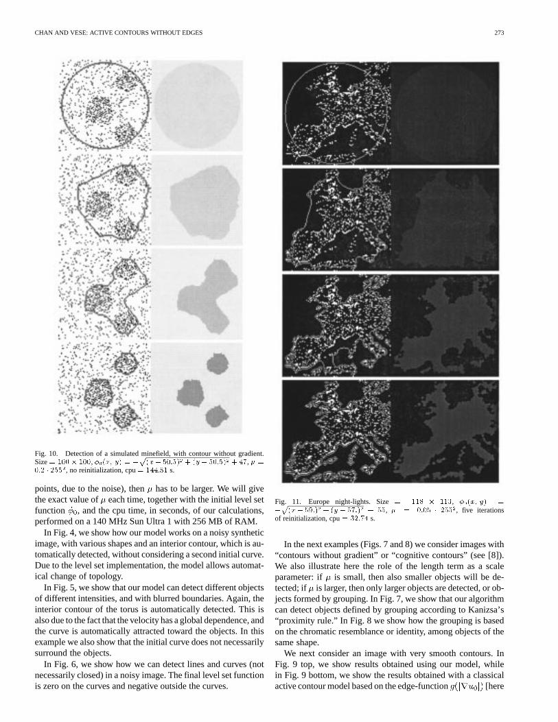
Fig. 10. Detection of a simulated minefield, with contour without gradient.Size= 100� 100, � (x; y) = � (x� 50:5) + (y � 50:5) + 47, � =0:2 � 255 , no reinitialization, cpu= 144:81 s.

points, due to the noise), thenhas to be larger. We will givethe exact value of each time, together with the initial level setfunction , and the cpu time, in seconds, of our calculations,performed on a 140 MHz Sun Ultra 1 with 256 MB of RAM.

In Fig. 4, we show how our model works on a noisy syntheticimage, with various shapes and an interior contour, which is au-tomatically detected, without considering a second initial curve.Due to the level set implementation, the model allows automat-ical change of topology.

In Fig. 5, we show that our model can detect different objectsof different intensities, and with blurred boundaries. Again, theinterior contour of the torus is automatically detected. This isalso due to the fact that the velocity has a global dependence, andthe curve is automatically attracted toward the objects. In thisexample we also show that the initial curve does not necessarilysurround the objects.

In Fig. 6, we show how we can detect lines and curves (notnecessarily closed) in a noisy image. The final level set functionis zero on the curves and negative outside the curves.

Fig. 11. Europe night-lights. Size= 118 � 113, � (x; y) =� (x� 59:) + (y � 57:) + 55, � = 0:05 � 255 , five iterationsof reinitialization, cpu= 32:74 s.

In the next examples (Figs. 7 and 8) we consider images with“contours without gradient” or “cognitive contours” (see [8]).We also illustrate here the role of the length term as a scaleparameter: if is small, then also smaller objects will be de-tected; if is larger, then only larger objects are detected, or ob-jects formed by grouping. In Fig. 7, we show that our algorithmcan detect objects defined by grouping according to Kanizsa’s“proximity rule.” In Fig. 8 we show how the grouping is basedon the chromatic resemblance or identity, among objects of thesame shape.

We next consider an image with very smooth contours. InFig. 9 top, we show results obtained using our model, whilein Fig. 9 bottom, we show the results obtained with a classicalactive contour model based on the edge-function [here


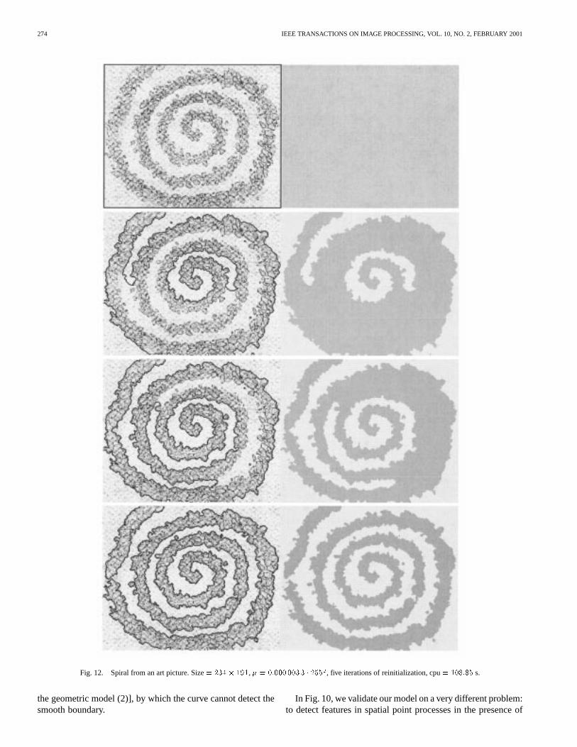
Fig. 12. Spiral from an art picture. Size= 234� 191, � = 0:0000033 � 255 , five iterations of reinitialization, cpu= 108:85 s.

the geometric model (2)], by which the curve cannot detect thesmooth boundary.

In Fig. 10, we validate our model on a very different problem:to detect features in spatial point processes in the presence of


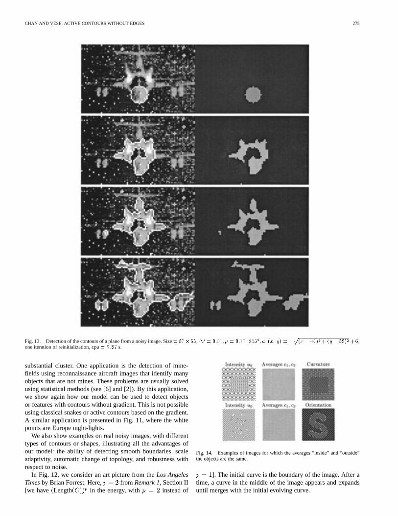
Fig. 13. Detection of the contours of a plane from a noisy image. Size= 87� 53,�t = 0:01,� = 0:17 � 255 , � (x; y) = � (x� 45) + (y � 39) +6,one iteration of reinitialization, cpu= 2:87 s.

substantial cluster. One application is the detection of mine-fields using reconnaissance aircraft images that identify manyobjects that are not mines. These problems are usually solvedusing statistical methods (see [6] and [2]). By this application,we show again how our model can be used to detect objectsor features with contours without gradient. This is not possibleusing classical snakes or active contours based on the gradient.A similar application is presented in Fig. 11, where the whitepoints are Europe night-lights.

We also show examples on real noisy images, with differenttypes of contours or shapes, illustrating all the advantages ofour model: the ability of detecting smooth boundaries, scaleadaptivity, automatic change of topology, and robustness withrespect to noise.

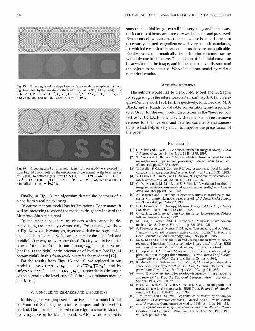
In Fig. 12, we consider an art picture from theLos AngelesTimesby Brian Forrest. Here, from Remark 1, Section II[we have Length in the energy, with instead of

Fig. 14. Examples of images for which the averages “inside” and “outside”the objects are the same.

]. The initial curve is the boundary of the image. After atime, a curve in the middle of the image appears and expandsuntil merges with the initial evolving curve.


Fig. 15. Grouping based on shape identity. In our model, we replacedu fromFig. 14 top left, by the curvature of the level curves ofu (Fig. 14 top right). Size= 64�64,� = 0:05 � 255 , � (x; y) = � (x� 32:5) + (y � 32:5) +30:5, 5 iterations of reinitialization, cpu= 10:20 s.

Fig. 16. Grouping based on orientation identity. In our model, we replacedufrom Fig. 14 bottom left, by the orientation of the normal to the level curvesof u (Fig. 14 bottom right). Size:64 � 64, � = 0:025 � 255 , � = 0:02 �255 , � (x; y) = � (x� 32:5) + (y � 32:5) + 30, five iterations ofreinitialization, cpu= 10:25 s.

Finally, in Fig. 13, the algorithm detects the contours of aplane from a real noisy image.

Of course that our model has its limitations. For instance, itwill be interesting to extend the model to the general case of theMumford–Shah functional.

On the other hand, there are objects which cannot be de-tected using the intensity average only. For instance, we showin Fig. 14 two such examples, together with the averages insideand outside the objects, which are practically the same (left andmiddle). One way to overcome this difficulty, would be to useother informations from the initial image , like the curvature(see Fig. 14 top right), or the orientation of level sets (see Fig. 14bottom right). In this framework, we refer the reader to [12].

For the results from Figs. 15 and 16, we replaced in ourmodel by curvature div , and byorientation respectively (the angleof the normal to the level curves). Other discriminants may beconsidered.

V. CONCLUDING REMARKS AND DISCUSSIONS

In this paper, we proposed an active contour model basedon Mumford–Shah segmentation techniques and the level setmethod. Our model is not based on an edge-function to stop theevolving curve on the desired boundary. Also, we do not need to

smooth the initial image, even if it is very noisy and in this way,the locations of boundaries are very well detected and preserved.By our model, we can detect objects whose boundaries are notnecessarily defined by gradient or with very smooth boundaries,for which the classical active contour models are not applicable.Finally, we can automatically detect interior contours startingwith only one initial curve. The position of the initial curve canbe anywhere in the image, and it does not necessarily surroundthe objects to be detected. We validated our model by variousnumerical results.

ACKNOWLEDGMENT

The authors would like to thank J.-M. Morel and G. Sapirofor suggesting us the references on Kanisza’s work [8] and Para-gios–Deriche work [20], [21], respectively, to R. Fedkiw, M. J.Black, and S. Ruuth for valuable conversations, and especiallyto S. Osher for the very useful discussions in the “level set col-lective” at UCLA. Finally, they wish to thank all three unknownreferees for their general and detailed comments and sugges-tions, which helped very much to improve the presentation ofthe paper.

REFERENCES

[1] G. Aubert and L. Vese, “A variational method in image recovery,”SIAMJ. Numer. Anal., vol. 34, no. 5, pp. 1948–1979, 1997.

[2] S. Byers and A. Raftery, “Nearest-neighbor cluster removal for esti-mating features in spatial point processes,”J. Amer. Statist. Assoc., vol.93, no. 442, pp. 577–584, 1998.

[3] V. Caselles, F. Catté, T. Coll, and F. Dibos, “A geometric model for activecontours in image processing,”Numer. Math., vol. 66, pp. 1–31, 1993.

[4] V. Caselles, R. Kimmel, and G. Sapiro, “On geodesic active contours,”Int. J. Comput. Vis., vol. 22, no. 1, pp. 61–79, 1997.

[5] G. Dal Maso, J. M. Morel, and S. Solimini, “A variational method inimage segmentation: existence and approximation results,”Acta Matem-atica, vol. 168, pp. 89–151, 1992.

[6] A. Dasgupta and A. Raftery, “Detecting features in spatial point pro-cesses with cluster via model-based clustering,”J. Amer. Statist. Assoc.,vol. 93, no. 441, pp. 294–302, 1998.

[7] L. C. Evans and R. F. Gariepy,Measure Theory and Fine Properties ofFunctions. Boca Raton, FL: CRC, 1992.

[8] G. Kanizsa,La Grammaire du Voir. Essais sur la perception: DiderotEditeur, Arts et Sciences, 1997.

[9] M. Kass, A. Witkin, and D. Terzopoulos, “Snakes: Active contourmodels,”Int. J. Comput. Vis., vol. 1, pp. 321–331, 1988.

[10] S. Kichenassamy, A. Kumar, P. Olver, A. Tannenbaum, and A. Yezzy,“Gradient flows and geometric active contour models,” inProc. Int.Conf. Computer Vision, Cambridge, MA, 1995, pp. 810–815.

[11] M.-S. Lee and G. Medioni, “Inferred descriptions in terms of curves,regions and junctions from sparse, noisy binary data,” inProc. IEEEInt. Symp. Computer Vision, Coral Gables, FL, 1995, pp. 73–78.

[12] C. Lopez and J. M. Morel, “Axiomatization of shape analysis and ap-plication to texture hyper discrimination,” inProc. Trento Conf. SurfaceTension Movement Mean Curvature, Berlin, Germany, 1992.

[13] R. Malladi, J. A. Sethian, and B. C. Vemuri, “A topology independentshape modeling scheme,” inProc. SPIE Conf. Geometric Methods Com-puter Vision II, vol. 2031, San Diego, CA, 1993, pp. 246–258.

[14] , “Evolutionary fronts for topology-independent shape modelingand recovery,” inProc. 3rd Eur. Conf. Computer VisionStockholm,Sweden, 1994, vol. 800, pp. 3–13.

[15] R. Malladi, J. A. Sethian, and B. C. Vemuri, “Shape modeling with frontpropagation: A level set approach,”IEEE Trans. Pattern Anal. MachineIntell., vol. 17, pp. 158–175, Feb. 1995.

[16] J. M. Morel and S. Solimini,Segmentation of Images by VariationalMethods: A Constructive Approach. Madrid, Spain: Revista Matem-atica Universidad Complutense de Madrid, 1988, vol. 1, pp. 169–182.

[17] , Segmentation d’Images par Méthode Variationnelle: Une PreuveConstructive d’Existence. Paris, France: C.R. Acad. Sci. Paris, 1989,vol. 308, pp. 465–470.


[18] D. Mumford and J. Shah, “Optimal approximation by piecewise smoothfunctions and associated variational problems,”Commun. Pure Appl.Math, vol. 42, pp. 577–685, 1989.

[19] S. Osher and J. A. Sethian, “Fronts propagating with curvature-depen-dent speed: Algorithms based on Hamilton–Jacobi Formulation,”J.Comput. Phys., vol. 79, pp. 12–49, 1988.

[20] N. Paragios and R. Deriche, “Geodesic Active Regions for Texture Seg-mentation,” INRIA RR-3440, 1998.

[21] , “Geodesic active regions for motion estimation and tracking,”INRIA RR-3631, 1999.

[22] E. Rouy and A. Tourin, “A viscosity solutions approach to shape-from-shading,”SIAM J. Numer. Anal., vol. 29, no. 3, pp. 867–884, 1992.

[23] L. Rudin, S. Osher, and E. Fatemi, “Nonlinear total variation based noiseremoval algorithms,”Phys. D, vol. 60, pp. 259–268, 1992.

[24] K. Siddiqi, Y. B. Lauziére, A. Tannenbaum, and S. W. Zucker, “Area andlength minimizing flows for shape segmentation,”IEEE Trans. ImageProcessing, vol. 7, pp. 433–443, Mar. 1998.

[25] M. Sussman, P. Smereka, and S. Osher, “A level set approach for com-puting solutions to incompressible two-phase flow,”J. Comput. Phys.,vol. 119, pp. 146–159, 1994.

[26] C. Xu and J. L. Prince, “Snakes, shapes and gradient vector flow,”IEEETrans. Image Processing, vol. 7, pp. 359–369, Mar. 1998.

[27] H.-K. Zhao, T. Chan, B. Merriman, and S. Osher, “A variational levelset approach to multiphase motion,”J. Comput. Phys., vol. 127, pp.179–195, 1996.

[28] H.-K. Zhao, S. Osher, B. Merriman, and M. Kang, “Implicit, nonpara-metric shape reconstruction from unorganized points using a variationallevel set method,” UCLA CAM Rep. 98-7, 1998.

[29] S. C. Zhu, T. S. Lee, and A. L. Yuille, “Region competition: unifyingsnakes, region growing, energy/bayes/MDL for multi-band image seg-mentation,” inProc. IEEE 5th Int. Conf. Computer Vision, Cambridge,MA, 1995, pp. 416–423.

Tony F. Chan (M’98) received the B.S. degree inengineering and the M.S. degree in aerospace engi-neering, both in 1973, from the California Instituteof Technology, Pasadena, and the Ph.D. degreein computer science from Stanford University,Stanford, CA, in 1978.

He is currently the Department Chair of the De-partment of Mathematics, University of California,Los Angeles, where he has been a Professor since1986. His research interests include PDE methods forimage processing, multigrid, and domain decomposi-

tion algorithms, iterative methods, Krylov subspace methods, and parallel algo-rithms.

Luminita A. Vese received the M.S. degree in mathe-matics from the University of Timisoara, Romania, in1993 and the M.S. and Ph.D. degrees in applied math-ematics, both from the University of Nice-Sophia An-tipolis, France, in 1992 and 1996, respectively. HerPh.D. subject was variational problems and partialdifferential equations for image analysis and curveevolution.

She held teaching and research positions at theUniversity of Nice, Nice, France, (1996–1997),the University of Paris IX, Paris, France, (1998),

and the Department of Mathematics, University of California (UCLA), LosAngeles (1997–2000). Currently she is computational and applied mathematicsAssistant Professor at UCLA. Her research interests include problems of curveevolution and segmentation using PDEs, variational methods, and level setmethods.

active contours without edges - image processing, ieee ...lvese/papers/ieeeip2001.pdf · chan and...

Documents