Gold Standard

Methodology to Estimate and Verify Averted Mortality and Disability

Adjusted Life Years (ADALYs) from Cleaner Household Air

Draft 0.1

November 2, 2016

Funded By

1

2

Table of Contents

Acknowledgments............................................................................................4Glossary...........................................................................................................5Introduction.....................................................................................................6Section I: Source and Applicability...................................................................7

1.1 Eligibility............................................................................................71.2 Overview of Methodological Approach..............................................9

Section II: Methodology for Characterizing Exposure....................................102. Project boundary..................................................................................103. Pollutants included in this methodology..............................................114. Baseline scenario monitoring...............................................................12

4.1 Baseline scenario definition............................................................124.2 Household survey............................................................................134.3 Personal exposure monitoring.........................................................134.4 Notation of special circumstances...................................................15

5. Project scenario monitoring.................................................................155.1 Project scenario definition...............................................................165.2 Household survey............................................................................165.3 Personal exposure measurement....................................................165.4 Technology usage monitoring (drop-off).........................................165.5 Carbon monoxide (CO) monitoring for charcoal-based interventions

175.6 Notation of special circumstances...................................................17

6. Monitoring guidelines...........................................................................176.1 Timing of first monitoring................................................................176.2 Personal exposure monitoring.........................................................176.3 Technology usage monitoring (drop-off).........................................19

Section III: Methodology for Converting to ADALYs.......................................191. HAPIT methodology and inputs............................................................192. Schedule for HAPIT maintenance and updating...................................22

Annex 1: Recommendations for applying the methodology..........................23Annex 2: Household survey and PEM monitoring guidelines.........................25Annex 3: Stove use monitoring (SUMs) use guidelines..................................35

3

Annex 4: HAPIT methods and assumptions...................................................37Annex 5: Key elements of conservativeness and non-conservativeness.......48

4

Acknowledgments

Several organizations and individuals have contributed to the development of this methodology.

Sincere thanks to:

ClimateCare: Tom OwinoSNV: Jason SteeleIndependent Consultant: Matt SpannagleGlobal Alliance for Clean Cookstoves: Sumi MehtaBerkeley Air Monitoring Group: David PenniseUC Berkeley: Ajay Pillarisetti, Prof. Kirk R. SmithWorld Bank: Rutu Dave, Tamer RabieWorld Vision Australia: Tim TempanyNexleaf Solutions Nithya Ramanathan, Jake Shual-BerkeRollins School of Public Health Prof. Thomas Clasen

The Author Team: Susan Anenberg, Prof. Patrick Kinney, Ken Newcombe, Vikash Talyan, Abhishek Goyal, Owen Hewlett

Gold Standard gratefully acknowledges the pioneering work of Prof. Kirk Smith and his team, including developing and piloting approach upon which this methodology is based.

We would also like to thank our funding partners Goldman Sachs, World Bank, Department of Foreign Affairs and Trade (Australian Aid) and World Vision-Australia for their support.

Enquiries should be directed to the Gold Standard at: info@goldstandard.org

5

Glossary

ADALY Averted disability-adjusted life year (also called DALY Averted)ALRI Acute lower respiratory infectionAF Adjustment factorCO2 Carbon dioxideCOPD Chronic obstructive pulmonary disorderDALY Disability-adjusted life yearGBD Global Burden of DiseaseGHG Greenhouse gasIER Integrated Exposure Response IHD Ischemic heart diseaseIHME Institute for Health Metrics and EvaluationISO International Organization for StandardizationHAPIT Household Air Pollution Intervention ToolLPG Liquefied petroleum gasPE Personal exposurePEM Personal exposure monitoringPM2.5 Particulate Matter less than 2.5 microns average diameter RAM Room area concentration monitoringSUMs Stove use monitoringYLD Years of life with disabilityYLL Years of life lostVER Voluntary emission reductionWHO World Health Organization

6

Methodology to Estimate and Verify Averted Mortality and Disability Adjusted Life Years (ADALYs) from Cleaner Household Air

This methodology is relevant to Sustainable Development Goal – 3 “Ensure healthy lives and promote well-being for all at all ages”

Draft Version 0.1, November 2, 2016

IntroductionThe development of this methodology was strongly informed by decades of evidence and experience from household air pollution exposure monitoring and epidemiological studies1, a proposed methodology for quantifying a saleable health product from household cooking interventions2 based on field work in Laos3 developed by UC Berkeley and Berkeley Air Monitoring Group, and the World Health Organization Indoor Air Quality Guidelines4.

This methodology uses exposure to fine particulate matter (PM2.5) as the best indicator of household air pollution. PM2.5 exposure causes negative health impacts, such as cardiovascular disease, respiratory disease, and lung cancer, all of which can end in premature death. It is considered to be the dominant contributor to the overall burden of disease from air pollution, no matter what the source.

The methodology focuses on measurements of personal exposure of households since measurements of pollution in particular places, such as the kitchen, are often poor indicators of actual exposure levels. 1 Smith KR, Bruce N, Balakrishnan K, Adair-Rohani H, Balmes J, Chafe Z, Dherani M, Hosgood HD, Mehta S, Pope D, Rehfuess E, and others in the HAP CRA Expert Group, Millions dead: how do we know and what does it mean? Methods used in the Comparative Risk Assessment of Household Air Pollution, Ann Rev of Public Health, 35: 185-206, 2014.2 Smith, K.R., A. Pillarisetti, L.D. Hill, D. Charron, S. Delapena, C. Garland, D. Pennise. (2015). Proposed Methodology: Quantification of a saleable health product (aDALYs) from household cooking interventions. University of California, Berkeley, and Berkeley Air Monitoring Group (funded by World Bank). Available at: http://ehsdiv.sph.berkeley.edu/krsmith/publications/2015/aDALY_Methodology.pdf, Accessed August 23, 2016.3 Hill L, Pillarisetti A, Delapena S, Garland C, Jagoe K, Koetting P, Pelletreau A, Boatman M, Pennise D, Smith K (2015) Air pollution and impact analysis of a pilot stove intervention: Report to the Ministry of Health and Inter-Ministerial Clean Stove Initiative of the Lao People’s Democratic Republic, University of California, Berkeley, and Berkeley Air Monitoring Group. Available at: http://ehsdiv.sph.berkeley.edu/krsmith/publications/2015/Lao_MoH_Main_report.pdf, Accessed September 28, 2016.4 World Health Organization (2014) Indoor Air Quality Guidelines: Household Fuel Combustion. WHO Guidelines for Indoor Air Quality. World Health Organization, Geneva, Switzerland. Available at: http://www.who.int/indoorair/guidelines/hhfc/en/, Accessed August 23, 2016.

7

Section I: Source and Applicability

1.1 EligibilityThis methodology is applicable to project activities that introduce technologies and/or practices for household thermal energy requirements and lighting that reduce household air pollution exposures and associated risk of harmful health impacts as compared to the baseline situation. These are termed “cleaner” in the rest of this document.

Projects that lead to verifiable reduction in PM2.5 exposure levels via a change in household energy use and/or emissions for cooking, heating, lighting are eligible under this methodology. Projects shall include cleaner cooking devices, fuels, or practices (e.g. improved application of eligible technologies, a shift from solid fuel or kerosene to biogas, etc.).

In addition to the cooking improvements which are required to be eligible for this methodology, the project may also include technologies such as solar lighting that lead to additional PM2.5 exposure reductions and count these exposure reductions in the health benefit calculation. Projects that improve/enhance ventilation of indoor air only (i.e., there is no improvement in technology, fuel, or practices) are not currently eligible.

Throughout the methodology, the term “technologies” is used to refer to both new technologies, fuel, and practices surrounding the use of the new technology.

Examples of eligible technologies include cleaner cookstoves (including biomass5, biogas, ethanol, other biofuels like plant oils and dimethyl ether derived from 100% renewable feedstock, and other modern fuel stoves such as LPG, natural gas, electric stoves, and electromagnetic induction cookstoves, etc,), space and water heaters (solar and otherwise), heat retention cookers, solar cookers and safe water supply and treatment technologies. Projects that involve a fuel switch to coal, charcoal, or kerosene are not eligible. Projects leading to greater efficiency in use of coal or kerosene compared to the baseline are also not eligible for this methodology.6 However, projects leading to more efficient use of charcoal compared to the baseline are eligible. Safe water supply and treatment technologies are only eligible if in the baseline situation solid fuels are burned to treat drinking water (e.g. boiling water).

5 Unprocessed biomass and biomass briquettes produced from agricultural waste such as coconut shell, sawdust etc or derived from dedicated biomass feedstock are eligible.6 These fuels are discouraged by the World Health Organization. World Health Organization (2014) Indoor Air Quality Guidelines: Household Fuel Combustion. WHO Guidelines for Indoor Air Quality. World Health Organization, Geneva, Switzerland. Available at: http://www.who.int/indoorair/guidelines/hhfc/en/, Accessed August 23, 2016.

8

These eligibility criteria reflect what is currently known of the potential benefits of different technology and various interventions. Additional types of interventions may be included in the future as additional information becomes available.

In the case of cleaner cookstoves and heating stoves, the project activities using this methodology shall meet the following conditions for the project technology:

Minimum 20% thermal efficiency based on lab test using the latest version of Water Boiling Test (WBT) protocol7;

Inclusion of incentive mechanism(s) to discourage the parallel use of baseline technology8 (actual discontinuity of baseline technology use not required); and

Evaluation criteria to avoid double counting of same project technology in other activities.

Projects that include modern fuels (e.g. liquefied petroleum gas, LPG and electricity derived from fossil fuels) can substantially reduce PM2.5 exposures and are eligible for this methodology. However, all projects shall adhere to Gold Standard Version 3.0 Safeguarding Principles (when finalized).

Important issues to consider when applying for this methodology are described in Annex 1.

1.2 Overview of Methodological ApproachThis methodology describes the quantification approach to be used to calculate health benefits from reductions in PM2.5 exposures resulting from the introduction of these technologies and related practices. PM2.5 related health impacts are quantified by use of published exposure-response relations that link PM2.5 levels to five major diseases established as related to air pollution exposure (stroke, ischemic heart disease, chronic obstructive pulmonary disease, lung cancer, and acute lower respiratory infection) (See Annex 4). These produce outcomes in terms of premature deaths expected 7 Water Boiling Test (WBT) available at http://cleancookstoves.org/technology-and-fuels/testing/protocols.html 8 Using the baseline technology as a backup or auxiliary technology in parallel with the cleaner technology introduced by the project activity is permitted as long as a mechanism is put into place to encourage the removal of the old technology (e.g. discounted price for the cleaner technology) and the definitive discontinuity of its use. The project documentation must provide a clear description of the approach chosen and the monitoring plan must allow for a good understanding of the extent to which the baseline technology is still in use after the introduction of the cleaner technology. For example, whether the existing baseline technology is or is not surrendered at the time of the introduction of the clean technology, or whether a new baseline technology is acquired and put to use by targeted end users during the project crediting period. The success of the mechanism put into place must therefore be monitored, and the approach must be adjusted if proven unsuccessful.

9

for each disease at the pollution level before intervention and after, the difference being averted by the intervention.

As deaths of children are not easily added to those for adults and the non-lethal impacts vary by disease, the methodology also produces results for Disability-Adjusted Life Years (DALYs), which include both years of life lost due to early death and years of healthy life lost due to onset of disease. The DALY is thus a single metric that combines both mortality and morbidity. It is a common metric used by public health and development entities globally as a way of comparing the burden of disease due to various risk factors and to evaluate and compare the effectiveness of health-related interventions, particularly when comparing different age groups and disease types. Using the DALY metric therefore enables the development of methodologies to quantify the health benefits of other types of public health interventions (e.g. water and sanitation) using a common and comparable metric. Averted DALYs (ADALYs, alternatively called DALYs averted) and averted mortality are the metrics used to quantify the health benefit of reduced PM2.5 exposures achieved from project implementation.

This methodology requires a two-step process wherein project developers shall:

1) monitor personal PM2.5 exposures before and after the project technology is introduced, and

2) convert monitored PM2.5 exposures to ADALYs using a web-based computer model based on current health literature called HAPIT – Household Air Pollution Intervention Tool.

Project developers shall use field monitored baseline and project PM2.5 exposure levels as inputs into HAPIT (available at: https://hapit.shinyapps.io/HAPIT/). HAPIT uses epidemiologically derived exposure-response9 functions to convert the monitored change in exposure to ADALYs.10 HAPIT only functions if local measurements are available, but does adjust output according to national or subnational conditions including background disease rates. Project developers must also monitor technology use to ensure that ADALYs are only calculated for the population using the technology. 9 Burnett RT, Pope CA III, Ezzati M, Olives C, Lim SS, Mehta S, Shin HH, Singh G, Hubbell B, Brauer M, Anderson HR, Smith KR, Balmes JR, Bruce NG, Kan H, Laden F, Prüss-Ustün A, Turner MC, Gapstur SM, Diver WR, Cohen A. 2014. An integrated risk function for estimating the global burden of disease attributable to ambient fine particulate matter exposure. Environ Health Perspectives 122:397–403; http://dx.doi.org/10.1289/ehp.130704910 Pillarisetti, A., S. Mehta, K. Smith. (2016). HAPIT, the Household Air Pollution Intervention Tool, to Evaluate the Health Benefits and Cost-Effectiveness of Clean Cooking Interventions. In E. Thomas (Ed), Broken Pumps and Promises: Incentivizing Impact in Environmental Health (pp. 147-169). Switzerland: Springer International Publishing.

10

Section II: Methodology for Characterizing Exposure

2. Project boundaryThe project developer shall provide clear definitions of the project boundary.11

In most cases, only members of the households (i.e. family members living in household permanently) targeted for the project technology may be included in the ADALYs calculation.

Although individual household PM2.5 emission reductions can substantially improve ambient air quality and positively affect health at community levels, community exposures may be difficult to attribute to the project, and ADALYs from ambient air quality improvements are therefore not included in this methodology. However, project developers can develop a rigorous and credible methodology to include community benefits (i.e., from reduced exposures to people beyond the project’s target households) and submit the methodology to the Gold Standard Foundation for review and approval. This should be discussed with Gold Standard at the earliest opportunity prior to development in order to ensure compatibility and viability with Gold Standard’s wider approach.

3. Pollutants included in this methodology The only pollutant addressed in this methodology is fine particulate matter (PM2.5). PM2.5 is a mixture of components, including black carbon, organic carbon, sulfates, nitrates and other trace components. Evidence is currently inconclusive regarding differential toxicity of individual components and mixtures on human health. Inefficient fuel combustion for cooking activities releases other harmful pollutants (e.g. carbon monoxide), but PM2.5 is the dominant contributor to the resulting public health impacts and has well-established exposure-response functions for multiple health outcomes. Therefore, total PM2.5 exposure is used as the indicator for calculating ADALYs from reduced exposure to household air pollution, and all other pollutants are excluded from this methodology.

This methodology sets forth methods for characterizing PM2.5 exposure from residential fuel combustion. PM2.5 exposure is not necessarily correlated with

11 The project boundary is the physical, geographical site of the baseline evaluation and the project technologies. This boundary could also host the baseline and project fuel collection and production (e.g. charcoal, plant oil) facilities associated with fuel processing, transportation.

11

stove PM2.5 emissions nor with monitored indoor PM2.5 concentrations. These terms are defined as follows:

Emissions: The rate of release of a pollutant per unit time or per unit of fuel. Often measured ‘directly’ from the combustion source and can be measured in the laboratory or the field.

Concentrations: The mass of a pollutant in a volume of air. Indoor concentrations result from the level of emissions, as well as the conditions of the room, such as ambient concentrations, ventilation rates, and processes, like deposition of the pollutant onto surfaces. Concentrations are usually measured in households in a particular room, such as the kitchen or living room, for example by placing a monitor on the wall of the kitchen for 24 hours. Concentration measurements do not account for the presence of people.

Exposures: The average concentration of a pollutant to which an individual or population is exposed over a specific period of time, accounting for their movement into and out of polluted microenvironments (e.g. between rooms and outdoors). Because human activity and corresponding exposure follows a diurnal pattern that may differ on different days, exposure should be monitored for at least a 48-hour period. If longer periods are chosen for monitoring exposure, they should be done in multiples of 24 hours after the first 48 hours.

In addition to reduced emissions from residential fuel combustion, some efficient technologies or practices may change the level of PM2.5 emissions produced during fuel production and transport. This may be the case, for example, where there is a change in fuel type from the baseline to the project scenario. Emissions released during fuel production, processing and transportation are excluded from this methodology because they are unlikely to substantially affect household-level PM2.5 exposures and it is not currently feasible to quantify upstream ADALYs.

4. Baseline scenario monitoringProject developers are required to conduct two studies for the baseline scenario: baseline household survey (Section 4.2) and personal exposure monitoring (Section 4.3). To ensure that the monitoring tests reflect normal conditions, households shall be instructed to follow their typical daily activity patterns during the monitoring. 4.1 Baseline scenario definition A baseline scenario is defined by the typical baseline fuel consumption pattern, PM2.5 exposures, and technology use in the population that is targeted to adopt the new project technology. This “target population” is used to calculate the representative baselines for the project activity.

12

For projects lasting longer than five years, the baseline scenario shall be reassessed every five years (i.e. a new round of baseline surveys and baseline personal exposure monitoring shall be conducted every five years).

Figure 1: Re-assessment of baseline personal exposures

4.2 Household surveyThe project developer shall conduct a baseline household survey prior to distribution of the project technology in the target population. The baseline surveys shall be carried out following the household survey guidelines, provided in Annex 2.4.3 Personal exposure monitoring Baseline and project PM2.5 exposure levels are a primary input to HAPIT for quantifying ADALYs (See Section III). Baseline personal exposure monitoring (PEM) of PM2.5 establishes the baseline exposure before the project technology is in use. PEM is only required in a sample of households in the target population (Annex 2).

For each of the sampled households, PEM shall be conducted for the primary cook for at least 48 continuous hours to capture diurnal and inter-day variation in cooking activities and exposure levels. PEM should be conducted in the season that is most representative of the full year or in a season that leads to conservative PEM value in the baseline scenario. Households in which the main cook smokes shall be excluded from the PEM sample, as the variability in personal exposure levels caused by smoking makes it difficult to

13

isolate the influence of the intervention. Similarly, houses using diesel generators, burning trash nearby, or experiencing other polluting sources that do not represent the conditions of the majority of the community should be excluded from the sample. The potential use of proxies in place of PEM for PM2.5 (e.g. carbon monoxide monitoring, room area monitoring, using exposure values from other studies) will be reassessed in the future.

PEM shall be done using either gravimetric monitoring alone or optical monitoring augmented by gravimetric monitoring. Gravimetric monitoring is more accurate than optical measurements because it directly measures PM2.5 mass, rather than a proxy based on light scattering measurements. Gravimetric (or “filter-based”) sampling uses a pump to draw air first through an inlet that removes particles larger than 2.5 micrometers, and then onto a filter that collects all of the remaining particles (i.e., PM2.5). The filter is weighed before and after sampling to calculate the integrated particle mass collected over the sampling time. This mass is then divided by the volume of air sampled to compute concentration in units of micrograms per cubic meter of air. However, gravimetric sampling requires expensive analytical balances for weighing filters and careful filter handling in a controlled laboratory.

Compared with optical monitors, gravimetric monitoring also typically requires study participants to wear more burdensome equipment. Optical (or “light scattering” of “nephelometry”) sampling estimates particle concentrations based on the amount of light scattered from a constant beam of light, and allows for near-continuous (e.g., minute by minute) monitoring using less burdensome equipment worn by study participants. However, studies show that optical monitors usually report values for PM2.5 that are biased either too high or too low as compared with gravimetric monitors. The direction and magnitude of the bias depends on the nature of the particles being monitored, the relative humidity, and other factors. Active sampling optical monitors with a defined size cut-point are typically more accurate than passive sampling optical monitors without a defined cut-point.

Where optical monitoring is used to measure exposures, an adjustment factor shall be applied to the measurements to correct for bias and convert them to “gravimetrically-equivalent” concentrations. The adjustment factor may vary by location, season, fuel type, and cooking practices, and thus shall be estimated in the relevant field setting. The adjustment factor is computed based on a set of at least 10 side-by-side 24 hour gravimetric and optical measurements, as described below. The correlation between the set of measurements reported by the two methods should exceed 0.75 in order to develop a valid adjustment factor; otherwise all PEM samples shall be monitored with gravimetric monitors.

Adjustment factor (AFoptical):14

Project developers using optical monitoring shall calculate an optical monitoring adjustment factor (AFoptical) as follows:

AFoptical=(meanPE gravimetric

mean PEoptical)

The AFoptical is the ratio of means for gravimetric and optical monitoring across all households that underwent monitoring. For optical monitoring, the mean of the optical signals during the monitoring period when the pump is on shall be applied. To estimate adjusted personal exposure (PEadjusted), the exposure measured by optical monitoring (PEoptical) shall then be multiplied by the AFoptical:

PEadjusted=PE optical∗AFo ptical

Adjusted personal exposure (PEadjusted) is used as the exposure input to HAPIT. Adjustment factors shall be developed separately in baseline and project scenarios to account for differences in aerosol composition due to changes in the primary cooking technology.

PEM is only required for the primary cook of the household. HAPIT uses default adjustment factors for other household members of 0.60 for non-cook adults and 0.85 for children, following methods used to calculate impacts in the IHME Global Burden of Disease project12,13 ).4.4 Notation of special circumstancesAt the time each household is monitored, a form should be completed to note any special circumstances in the household during monitoring (for example, cooking for a festival or large party or eating away from home). If the circumstances depart too far from normal, the monitoring session shall be repeated or the household shall be excluded from the sample.

5. Project scenario monitoringThe project developer shall conduct three studies to determine exposure reductions attributable to the project:

1. project household survey (Section 5.2) and12 Smith KR, Bruce N, Balakrishnan K, Adair-Rohani H, Balmes J, Chafe Z, Dherani M, Hosgood HD,Mehta S, Pope D, Rehfuess E, and others in the HAP CRA Expert Group, Millions dead: how do we know and what does it mean? Methods used in the Comparative Risk Assessment of Household Air Pollution, Ann Rev of Public Health, 35: 185-206, 2014.13 World Health Organization (2014) Indoor Air Quality Guidelines: Household Fuel Combustion. WHO Guidelines for Indoor Air Quality. World Health Organization, Geneva, Switzerland. Available at: http://www.who.int/indoorair/guidelines/hhfc/en/, Accessed August 23, 2016.

15

2. personal exposure monitoring (Section 5.3) and 3. technology usage monitoring (Section 5.4Error: Reference source not

found).4. projects involving charcoal-based interventions are also required to

conduct carbon monoxide (CO) room area monitoring (Section 5.5). Project monitoring shall occur no sooner than six months after the new technology is disseminated and shall be conducted in the same season as the baseline monitoring in locations where there are major seasonal variations.

As for baseline monitoring, households shall be instructed to follow their typical daily activity patterns during the monitoring. In case of paired sampling (before and after monitoring) if the technology is being used in a different location than in the baseline monitoring or if a different person is cooking (unless being done in a comparable way so as not to change the outcome), these data points should be excluded from the analysis. To account for this and other reasons that households may not end up being suitable for inclusion in monitoring, the initial monitoring sample size should be larger than the sample size required for PEM. 5.1 Project scenario definitionA project scenario is defined by the PM2.5 exposures and technology usage of end-users within the target population. PM2.5 exposure reductions are accounted for by comparing exposures in the project scenario to the baseline scenario.5.2 Household surveyThe project developer shall conduct a project household survey to determine how the project technology or practice is being implemented and whether household circumstances have changed. The project household survey shall be carried out following the household survey guidelines, provided in Annex 2 5.3 Personal exposure measurement PEM of PM2.5 shall be monitored in a sample of project households. Only households still using the project technology shall be included in the PEM sample to avoid averaging exposure levels with households not using the project technology and match the population used to calculate ADALYs. PEM monitoring shall be carried out for at least 48 continuous hours in each household in the monitoring sample. Optical measurements (PEoptical¿shall be adjusted to scale to gravimetric monitoring (PEgravimetric) values, following Section 4.3. 5.4 Technology usage monitoring (drop-off)

16

Project technology usage (simply whether it is being used at all or not) shall be monitored simultaneously with PEM via surveys or stove use monitors (SUMs) to determine the portion of project households still using the technology. A variety of SUMs are available and may be used following the guidelines provided in Annex 3. SUMs should be applied consistently to the project technology in each sampled household. The usage rate is applied in HAPIT to limit the ADALY calculations to just the households using the technology. The objective of technology use monitoring is to exclude the households that are no longer using the technology from the ADALY calculation.5.5 Carbon monoxide (CO) monitoring for charcoal-based interventionsCO levels above World Health Organization (WHO) air quality guidelines14 could result in adverse health effects. For charcoal-based interventions only, room area monitoring of CO is required in all households undergoing PM2.5 PEM. CO monitoring is required to run for 24 hours at a minimum in sample households. If the 24 hour average CO concentration exceeds the WHO 24hr CO concentration guideline i.e., 7 mg/m3 in a fraction of monitored households, the same fraction of project households in the total project population will no longer be eligible for claiming ADALYs.5.6 Notation of special circumstancesAs for baseline monitoring, a form to note special circumstances shall be used at the time each household is monitored as described in Section 4.4.

6. Monitoring guidelines Monitoring determines the extent to which PM2.5 exposure reductions and technology usage rates measured during project monitoring are maintained as the project is implemented over time. 6.1 Timing of first monitoring The first monitoring for the project scenario after distribution of the technology can be conducted any time after six months after start of use of the new technology in the households. 6.2 Personal exposure monitoringThe health benefits are based on the difference in exposure level between the baseline and project household data.

Please refer to Annex 2 for sampling approach and sample size requirements and guidelines for PEM monitoring.

14 World Health Organization (2014) Indoor Air Quality Guidelines: Household Fuel Combustion. WHO Guidelines for Indoor Air Quality. World Health Organization, Geneva, Switzerland. Available at: http://www.who.int/indoorair/guidelines/hhfc/en/, Accessed August 23, 2016.

17

PEM shall be conducted every other year (i.e. every second year) at a minimum. For the years in which no PEM is conducted (e.g. year 2, year 4, etc.), PEM values from the prior year shall be used with the usage rate from the current year (e.g. for year 2, year 1 PEM value shall be used with year 2 usage rate). To ensure that ADALYs are not over-allocated, 40% of issuable ADALYs calculated in the off-years (i.e. in which no PEM is conducted) will be held in reserve pending exposure measurements in the following year. If the following year’s monitored exposure levels are below those used in the off year, the 40% reserved ADALYs will be awarded back to the project. If the following year’s monitored exposure levels are higher than those used in the off year, such that the project was over-allocated ADALYs in the off year even after the 40% reserve, the difference will be subtracted from the following year’s ADALY issuance.

Figure 2: Allocation of ADALYs with biennial monitoring of personal exposure

6.3 Technology usage monitoring (drop-off)Technology usage monitoring is carried out to determine if the project technology is in use or not. The technology usage frequency or stacking (use of traditional stove in parallel with project technology) shall be captured through the PEM. Therefore the objective of usage monitoring is to

18

determine the fraction of users who have stopped using the project technology completely i.e., drop off. The project developer shall carry out the usage survey annually, or more frequently, and in all cases on time for any request of issuance. Usage monitoring provides a single usage parameter that is weighted based on drop off rates that are representative of the age distribution for project technologies in the total sales record.15 Please refer to Annex 2 for usage survey requirements and guidelines.

Section III: Methodology for Converting to ADALYs

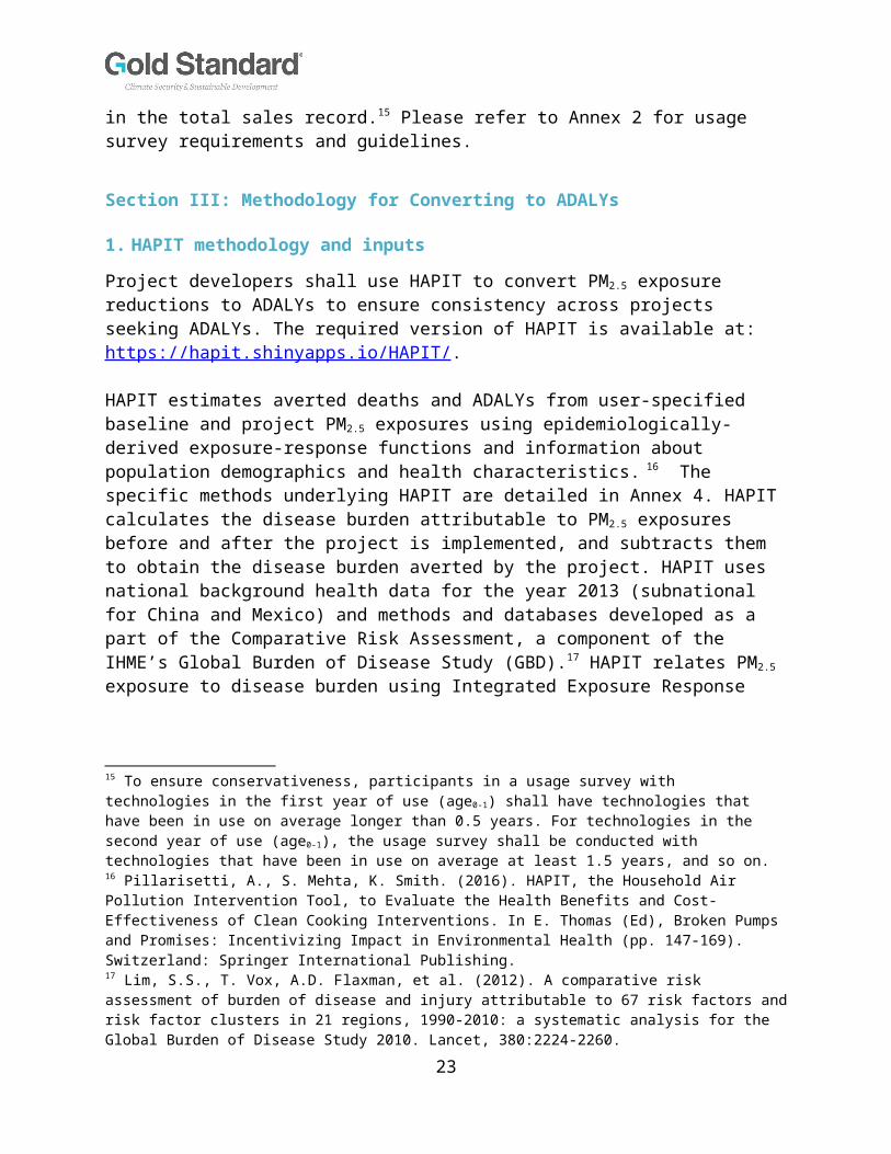
1. HAPIT methodology and inputsProject developers shall use HAPIT to convert PM2.5 exposure reductions to ADALYs to ensure consistency across projects seeking ADALYs. The required version of HAPIT is available at: https://hapit.shinyapps.io/HAPIT/.

HAPIT estimates averted deaths and ADALYs from user-specified baseline and project PM2.5 exposures using epidemiologically-derived exposure-response functions and information about population demographics and health characteristics. 16 The specific methods underlying HAPIT are detailed in Annex 4. HAPIT calculates the disease burden attributable to PM2.5 exposures before and after the project is implemented, and subtracts them to obtain the disease burden averted by the project. HAPIT uses national background health data for the year 2013 (subnational for China and Mexico) and methods and databases developed as a part of the Comparative Risk Assessment, a component of the IHME’s Global Burden of Disease Study (GBD).17 HAPIT relates PM2.5 exposure to disease burden using Integrated Exposure Response (IER) functions for the major disease categories associated with PM2.5 exposure.18

The five major disease categories for which HAPIT estimates ADALYs are:15 To ensure conservativeness, participants in a usage survey with technologies in the first year of use (age0-1) shall have technologies that have been in use on average longer than 0.5 years. For technologies in the second year of use (age0-1), the usage survey shall be conducted with technologies that have been in use on average at least 1.5 years, and so on. 16 Pillarisetti, A., S. Mehta, K. Smith. (2016). HAPIT, the Household Air Pollution Intervention Tool, to Evaluate the Health Benefits and Cost-Effectiveness of Clean Cooking Interventions. In E. Thomas (Ed), Broken Pumps and Promises: Incentivizing Impact in Environmental Health (pp. 147-169). Switzerland: Springer International Publishing.17 Lim, S.S., T. Vox, A.D. Flaxman, et al. (2012). A comparative risk assessment of burden of disease and injury attributable to 67 risk factors and risk factor clusters in 21 regions, 1990-2010: a systematic analysis for the Global Burden of Disease Study 2010. Lancet, 380:2224-2260.18 Burnett RT, Pope CA III, Ezzati M, Olives C, Lim SS, Mehta S, Shin HH, Singh G, Hubbell B, Brauer M, Anderson HR, Smith KR, Balmes JR, Bruce NG, Kan H, Laden F, Prüss-Ustün A, Turner MC, Gapstur SM, Diver WR, Cohen A. 2014. An integrated risk function for estimating the global burden of disease attributable to ambient fine particulate matter exposure. Environ Health Perspectives 122:397–403; http://dx.doi.org/10.1289/ehp.1307049

19

Ischemic heart disease (IHD) Stroke Chronic obstructive pulmonary disease (COPD) Lung cancer Child (under 5 years) acute lower respiratory infection (ALRI)

The IERs provide exposure-response relationships across the entire range of PM2.5 exposures (up to 1000 µg/m3) for each of these health endpoints. See Annex 4 for more details.

HAPIT will be updated regularly as per the GBD is updated to incorporate new evidence on health effects becomes available, and as population demographics changes, in consultation with the Gold Standard Technical Governance Committee. These changes may increase or decrease the ADALYs per unit reduction in PM2.5. Project developers will be issued ADALYs that are estimated by the version of HAPIT in use at the time of requesting issuance of ADALYs certificates.

HAPIT uses a variety of input parameters to estimate averted deaths and ADALYs. Parameters that are hard-wired into HAPIT and cannot be altered by the project developer include exposure-response functions, population, and baseline disease incidence rates (see Annex 4 and ).

Parameters that are required to be monitored and input by the project developer include baseline and project PM2.5 exposures, number of targeted households, fraction of targeted households using the intervention, percentage of project population using solid fuels and the useful intervention lifetime (). The user must also input the country where the project is located to use the appropriate national or subnational baseline health data. Projects in China and Mexico shall input the province or state where the project is located to use the subnational baseline health data published by the GBD study. Table 1. User-defined parameters required to run the HAPIT tool, along with their units and data sources.

Parameter Units Data SourceCountry or province/state where project is located

Country or province/state name

Country or province/state where the project is located

Baseline PM2.5 exposure µg/m3 PEM or alternative methods detailed in Section 4.3

Project PM2.5 exposure µg/m3 PEM or alternative methods detailed in Section 5.3

20

Number of targeted households

# Number of households targeted for inclusion in the intervention (includes households not utilizing the technology)

Number people per household # Household surveys or HAPIT default

Percentage of project population using polluting fuels (PFUfraction)

% Household surveys

Number children per household age under 5 years

# Household surveys or HAPIT default

Fraction of targeted households using intervention (usage rate)19

# (0 to 1) Household surveys and/or stove use monitoring (Section 5.4)

Useful intervention lifetime # years Manufacturer specification

Outputs from HAPIT are the reduction in mortality and DALYs among the population from reduced PM2.5 exposure achieved during each year of the project’s operation. As HAPIT runs in full calendar year increments, results output by HAPIT shall be multiplied by the weighted average fraction of days of the year during which the project stoves were operational. Long-term health benefits associated with each year’s exposure reduction are still included in the annual estimates and will be awarded to the project in the year exposure was reduced (i.e. for exposure reduction in year 2016, associated health benefits in year 2016-2020 are awarded in 2016). ADALYs and avoided mortality will be awarded to projects each year of the project’s lifetime using the monitored exposures and usage rates as per monitoring requirements. These benefits would be expected regardless of whether exposure levels return to baseline in the next year. For conservativeness, HAPIT will calculate health benefits for only the five years following a one-year exposure reduction, or 80% of the total health benefits that would be expected over the 20 years following the one-year exposure reduction based on US EPA cessation lag.20 The total health benefits for the project are the sum of the 5-year health benefits accrued for each year of exposure reduction (i.e. 5-year health benefits for exposure reduction in 1 year + 5-

19 It does not account for the fraction of baseline technology use that is displaced by the new technology. In other words, usage fraction incorporates any household using the new technology at all, regardless of how much the new technology is used and how much the baseline technology is used.20 U.S. Environmental Protection Agency – Science Advisory Board. 2004. Advisory Council on Clean Air Compliance Analysis Response to Agency Request on Cessation Lag. EPA-COUNCIL-LTR-05-001. December. Available at: https://yosemite.epa.gov/sab%5CSABPRODUCT.NSF/39F44B098DB49F3C85257170005293E0/$File/council_ltr_05_001.pdf, Accessed October 17, 2016.

21

year health benefits for exposure reduction in year 2, and so on through the project’s lifetime).

2. Schedule for HAPIT maintenance and updatingHAPIT is planned to be updated as the evidence relating PM2.5 exposure to individual health outcomes evolves, as assessed on an ongoing basis by the Global Burden of Disease (GBD) project.21 The HAPIT version required by this methodology is expected to be updated annually to incorporate updated baseline incidence rates and at least every five years to incorporate changes in the PM2.5 exposure-response functions.

21 As the GBD is the broadest and most rigorous assessment of the health literature for household air pollution, this methodology will rely on GBD for evaluating the weight of the evidence for including or excluding individual health endpoints and their exposure-response functions.

22

Annex 1: Recommendations for applying the methodologyThis annex provides key issues to consider when applying for this methodology.

Potential cost-effectiveness based on stove performance and usageProjects using cookstoves that do not substantially reduce PM2.5 emissions and those using cookstoves that have low usage rates and/or rates of displacing the baseline technology will produce a substantially and disproportionately smaller number of ADALYs per household due to the non-linear nature of the exposure-response curves. Project developers using these technology types should carefully assess the cost-effectiveness of using this methodology.

For IHD, stroke, and ALRI, the IERs flatten out substantially at the high PM2.5 exposures typically found in households that burn solid fuels inefficiently indoors. Since IHD, stroke, and ALRI are the main contributors to household PM2.5-related ADALYs, the flattening of the exposure-response curve at high exposures indicates that for individual exposure at these high levels, incremental reductions in PM2.5 exposure will not yield substantial health benefits or estimated ADALYs. For projects using cookstoves that do not substantially reduce PM2.5 exposures or for any technology that does not displace the traditional stove for the majority of cooking time, project developers should expect these conditions to result in a low number of ADALYs.

Pre-assessment of project technology usage and durabilityProject developers are encouraged to assess the usage, stacking, and technology survival and durability for the planned project technology in the target population prior to undertaking the project and conducting project monitoring. The new technology chosen for dissemination should meet the needs of the target population (including local cooking patterns and fuel availability) and should have low pollutant emissions.

The number of ADALYs that can be awarded to a project depend on both the new technology substantially displacing baseline stove use and on the degree to which the new technology reduces PM2.5 emissions. Even if the project technology is very clean, if it does not substantially displace use of the baseline technology, the project may only be awarded a small number of ADALYs. Project developers should, therefore, only proceed to project implementation and monitoring after usage, stacking, and survival of the project technology is found acceptable.

23

As a general rule, the project technology may be considered acceptable if it displaces at least 80% of the baseline technology use and if less than 10% of households experience technology failure over the period monitored. Additional quantitative guidance is given by Johnson et al. (2015).22 Protocol for determining durability is available at the Global Alliance for Clean Cookstove website. If the project technology does not meet the above guidelines for acceptable usage and durability, project developers should evaluate whether a different approach or technology is needed to increase the chances that the project will successfully reduce PM2.5 exposures and yield ADALYs.

If verification results do not meet the above guidelines for baseline technology displacement and new technology survival, the project developers should reconsider whether to seek annual verification of ADALYs. Project developers who do not assess technology usage and viability prior to starting the project, therefore, are incurring a risk that the project will not yield sufficient ADALYs.

22 Johnson, Michael A., et al., 2015, "Quantitative guidance for stove usage and performance to achieve health and environmental targets." Environmental Health Perspectives 123.8: 820-826.

24

Annex 2: Household survey and PEM monitoring guidelines

1.0 Survey Guidelines The household surveys are required for analyzing both baseline and project scenario. The following guidelines are to assist planning and conducting successful household surveys and personal exposure monitoring (PEM) of PM2.5.

In every household participating in the study, a consent form should be administered that guarantees data privacy, low risk from the equipment, non-responsibility for loss or damage to the equipment, and the ability to withdraw from the study at any time without penalty. Any data form showing personal identifiers (name, household number, address, etc.) should be kept locked away by the project field manager. Personal identifiers should not be entered into the database that will be available for analysis. Instead, households should be identified in the database only by ID numbers, with the code linking these numbers to personal identifiers kept locked away by the project field manager.

In a similar fashion, no photos should be taken in which individuals can be identified without an oral consent. If the intention is to use the photo in publications, websites, or project reports, a written consent should be on file, although the person does not actually have to personally sign in illiterate populations (fieldworker can sign and date in their stead after oral consent is given).

Survey and monitoring activities may be exempt from ethics and/or Institutional Review Board (IRB) clearance if the results are used exclusively to assess programme performance and do not constitute research designed to develop or contribute to generalizable knowledge. Local requirements should be consulted. If survey and monitoring activities are not exempt, then the programme developer is obligated to secure such clearance.

The project developer should conduct the household surveys in accordance with the steps listed below.

A provisional first estimate should be made of fuel mix utilized in each households, in the sense of how they are apportioned. For example, it may be determined that some customers use dung and wood in approximately equal measure, while others use only wood or only charcoal. If fuel mixing is prevalent in target households, a project developer shall treat each fuel group as separate. An initial assessment should also be made of other factors which determine fuel consumption patterns that may influence the emission profile of the household. This, for example, includes characteristics

25

such as whether the households are cooking commercially or for domestic consumption only, whether the households cook indoors or outdoors or both, whether the kitchen is separate from or attached to the main house, whether there is significant variation in seasons, whether they are doubling cook-stoves as space-heaters or not, whether they are collecting fuel manually or purchasing it and so on. Steps 1 to 3 should be followed for this provisional first estimate.

1.1 Baseline household surveys

Step 1: Establish a pilot distribution record:A pilot distribution and installation is useful to collect data for the population that is targeted by the project technology. The developer shall randomly pick the households who could be the subjects of pilot surveys for characterising cooking, heating and lighting practices.

Step 2: Provisionally assess fuel types, baseline technology, fuel mix, and kitchen regimes: Project developers shall specify the fuels and energy sources used in the pilot households, in both the baseline and project scenarios, dividing them into the fuel type categories such as firewood, charcoal, biogas, LPG, kerosene, dung, agriculture residue, fuel mix, etc. The pilot surveys shall be carried out in minimum 30 households.

Step 3: Divide pilot distribution record into customer groups:Having provisionally distinguished the factors that determine emission profiles of the pilot households, the project proponent should divide the total distribution record into major end user groups displaying distinct patterns of fuel consumption and stove type. It is not necessary to split the distribution record into different end-user groups at this stage if no obvious major distinctions exist.

The above assessment is provisional, allowing the target population to be divided into major end user groups each of which will then be analysed in more detail, through baseline surveys (see steps 4 and 5 below) with respect to the characteristics set out here.

Step 4: Carryout the qualitative baseline survey: The baseline survey should be carried out for each major group of end user (each group provisionally assessed), randomly selected from the relevant set of customers on the distribution Record, following these guidelines as to minimum sample size:

Group size < 300: Minimum sample size 30 Group size 300 to 1000: Minimum sample size 10% of group size Group size > 1000 Minimum sample size 100

26

The baseline survey involves observations and questionnaires undertaken by an expert survey team visiting target households. A sample outline of questionnaire is available in Appendix 1.

Step 5: Refine demarcation of end user groups and populate Project Database: The results of the baseline survey are used to revise the provisional groupings, if any, made in step three above. The determination of groups allows individual distribution in the distribution record to be sorted properly in the Project Database.

The Project Database is simply the distribution record re-organised for calculation of health benefits. Since the exposure level determining health benefits are specific to each end user group, the Project Database should contain distinct lists for each group, wherever this is possible.

The baseline survey should conclude with a formal report on its findings. It will typically conclude with a set of end-user groups, for further consideration during the project design process.

1.2 Project household surveys:Similar to baseline surveys, annual project surveys are conducted with end users representative of the project scenario target population. The annual project survey results will allow developers to identify changes over time in a project scenario. It provides critical information on year-to-year trends in end user characteristics such as technology use, type of fuel use, kitchen characteristics and seasonal variations. The project survey has the same sample sizing and data collection guidelines as the baseline survey described above in Step 4. The project surveys can be conducted with usage survey participants, however the sample size and sampling strategy shall meet the requirements of usage surveys.

1.3 Usage Survey Guidelines Usage survey is an annual event which results in a usage parameter to account for drop off rates as project technologies age and are replaced.23 A usage parameter is required that is weighted to be representative of the quantity of project technologies of each age being credited in a given project scenario. For example, if only technologies in the first year of use (age0-1) are being credited, a usage parameter shall be established through a usage survey for technologies age0-1. If an equal number of technologies in the first year of use (age0-1) and second year of use (age1-2) are credited, a usage

23 It may be the case that the drop off rate is lower in the second year than in the first year, reflecting possible difficulties in the early adoption of a new technology.

27

parameter is required that is weighted to be equally representative of drop off rates for technologies age0-1 and age1-2. The minimum total sample size required for usage surveys is 100, with at least 30 samples for project technologies of each age being credited.24 Any sampling methods can be used, provided that the sample is selected randomly. Most common sampling approaches are discussed in Guidelines for sampling and surveys for CDM project activities and programme of activities. Usage surveys shall be conducted in person and should include observation by the interviewer within the household in question.

If using surveys to determine usage rate, the majority of interviews in a usage survey shall be conducted in person and include expert observation by the interviewer within the kitchen in question, while the remainder may be conducted via telephone by the same interviewers on condition that in-kitchen observational interviews are first concluded and analysed such that typical circumstances are well understood by the telephone interviewers.

Annual usage survey and project surveys can be carried out together provided that the sample size and sampling strategy requirements of the usage survey are met.

(Detailed Usage Survey Guidelines are currently being developed that will be referenced for use along with these guidelines.)

2.0 PEM monitoring Guidelines It is recommended that an experienced professional group be engaged to conduct the air pollution monitoring that is part of the ADALYs quantification methodology. Here, however, we note just a few of the major issues that need to be considered when doing such monitoring.

• Before beginning, a group of local women should be requested to choose among the available methods to carry personal monitors (backpack, sling, hip pack, or shoulder pouch) to optimize comfort and cultural acceptance.

Personal exposure measurements should only be done with non-pregnant women, 18 years or older.

Survey and monitoring activities may be exempt from ethics/ Institutional Review Board (IRB) clearance if the results are used exclusively to assess programme performance and do not constitute

24 Thus if technologies of age 1-5 are credited, the usage survey shall include 30 representative samples from each age for a total of 150 samples. The resulting usage parameter should be weighted based on the proportion of technologies in the total sales record of each age.

28

research designed to develop or contribute to generalizable knowledge. Local requirements should be consulted. If survey and monitoring activities are not exempt, then the programme developer is obligated to secure such clearance.

For each of the sampled households, PEM shall be conducted for the primary cook for at least 48 continuous hours to capture diurnal and inter-day variation in cooking activities and exposure levels

The approach taken to conduct the PEM tests must in any case be such that:

- it is transparent and can easily be replicated, - the sample is selected so as to be representative of the larger

population of households adopting the technology for baseline scenario and technology users in project scenario. This is most often achieved by random sampling (see below),

- the impact of daily and seasonal variations on the expected PEM is accounted for,

- at the time each household is monitored, a form should be completed to note any special circumstances in the household during monitoring (for example, cooking for a festival or large party or eating away from home). If the circumstances depart too far from normal, the monitoring session shall be repeated or the household excluded from the sample.

All relevant guidelines dictating such field studies in the countries in which measurements will be made should be followed.

2.1 Sampling approach Project developers may opt to use either a “before-after” design (paired sampling) or a cross-sectional design (unpaired sampling). Simple random sampling approaches can be applied for PEM monitoring within a particular project scenario (same cookstove is used as project technology). Simple random sample can be taken from the entire population for a particular project scenario with population having different vintages (age group e.g. 0-1 year, 1-2 years, 2-3 years and so on) of same stoves with at least total 30 samples. Alternate approaches like cluster sampling, stratified sampling etc. can be used with justification.

2.2 Sample sizeBaseline and project monitoring sample sizes for PEM are based on statistical approaches for health studies as provided in the table below. 90/30 confidence / precision level25 (i.e., the end-points of the 90% confidence interval of the mean lie within +/- 30% of the estimated mean), is required for exposure reductions monitored using PEM. A two-sided test should be applied to 90 / 30 check. A minimal sample size of 30 households should be 25 https://ump.pnnl.gov/showthread.php/5106-2.3-Confidence-and-Precision

29

used for sampling, and conservative bound of the confidence interval shall be used if the statistical precision is not met. This means that in case of baseline PEM if the statistical precision is not met the mean PEM value should be adjusted with two sided lower bound of the error and vice-versa for project scenario PEM. Since a normal distribution curve is generally not obtained for PEM, the 90/30 precision shall be applied to log-transformed values for PEM. An example to illustrate 90/30 confidence/precision check approach is provided in Appendix -2.

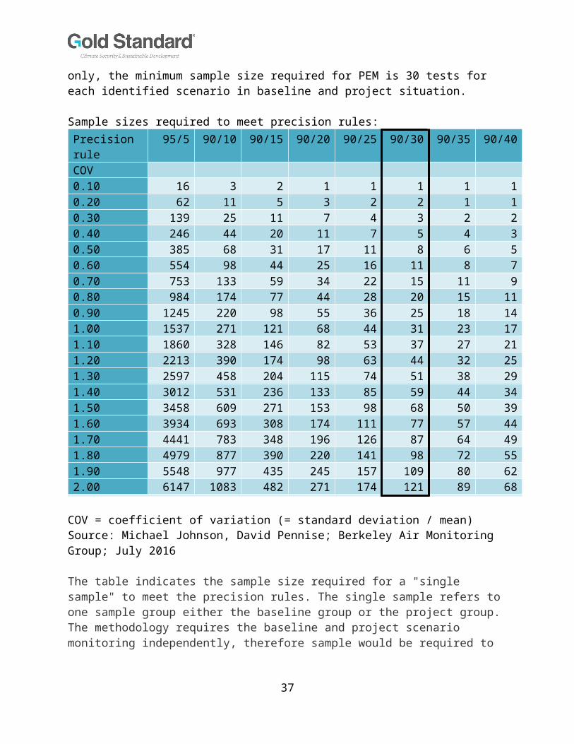
The following table delineates the size of the samples required from the target population for paired designs (before-and-after with no control group) and un-paired (cross-sectional) designs to evaluate personal exposure for new compared to baseline technologies. These sample sizes are indicative for baseline and project PEM. It shall be noted that it is an indicative list only, the minimum sample size required for PEM is 30 tests for each identified scenario in baseline and project situation.

Sample sizes required to meet precision rules:Precision rule

95/5 90/10 90/15 90/20 90/25 90/30 90/35 90/40

COV  0.10 16 3 2 1 1 1 1 10.20 62 11 5 3 2 2 1 10.30 139 25 11 7 4 3 2 20.40 246 44 20 11 7 5 4 30.50 385 68 31 17 11 8 6 50.60 554 98 44 25 16 11 8 70.70 753 133 59 34 22 15 11 90.80 984 174 77 44 28 20 15 110.90 1245 220 98 55 36 25 18 141.00 1537 271 121 68 44 31 23 171.10 1860 328 146 82 53 37 27 211.20 2213 390 174 98 63 44 32 251.30 2597 458 204 115 74 51 38 291.40 3012 531 236 133 85 59 44 341.50 3458 609 271 153 98 68 50 391.60 3934 693 308 174 111 77 57 441.70 4441 783 348 196 126 87 64 491.80 4979 877 390 220 141 98 72 551.90 5548 977 435 245 157 109 80 622.00 6147 1083 482 271 174 121 89 68

COV = coefficient of variation (= standard deviation / mean) Source: Michael Johnson, David Pennise; Berkeley Air Monitoring Group; July 2016

30

The table indicates the sample size required for a "single sample" to meet the precision rules. The single sample refers to one sample group either the baseline group or the project group. The methodology requires the baseline and project scenario monitoring independently, therefore sample would be required to meet the precision rule for the baseline and project groups independently.

2.3 Statistical analysisBefore beginning the analysis, be sure to check for “outliers”, i.e. values which are very different to the majority of the sample. Outliers should be examined to check for mistakes with data recording, or investigated to ascertain if there were unusual circumstances which led to that result. If so, then the observation should be removed or corrected before the analysis and it shall be justified and recorded in the monitoring report. One way to identify potential outliers is to produce a box plot of the data. Most statistical software enables this. Any points which are plotted individually on the box plot are candidates for outliers and should be investigated. Equivalently, potential outliers can be identified as those points which are either greater than 1.5 times the inter quartile range (IQR) from the third quartile, or less than 1.5 times the IQR from the first quartile.

3.0 Sampling approaches Any sampling methods can be used, provided that the sample is selected randomly. Most common sampling approaches are discussed in Guidelines for sampling and surveys for CDM project activities and programme of activities. A few most relevant approaches are discussed below.

3.1 Simple random samplingA simple random sample is a subset of a population (e.g. villages, individuals, households) chosen randomly, such that each household has the same probability of being selected. The sample-based estimate (mean or proportion) is an unbiased estimate of the population parameter.

Simple random sampling is conceptually straightforward and easy to implement – provided that a sampling frame of all households of the population exists. Its simplicity makes it relatively easy to analyse the collected data.

Simple random sampling is suited to populations that are relatively homogeneous in terms of factors that influence household air pollution (such as urban vs. rural, fuel types, kitchen types, ethnicity, and socioeconomic circumstances). In many instances a large population size and dispersed

31

nature of population may cause a lack of homogeneity, while in some cases those factors may have relatively low impact on homogeneity. The costs of data collection under simple random sampling could be higher than other sampling approaches when the population is large and geographically dispersed.

3.2 Stratified random samplingWhen the population under study is not homogeneous but instead consists of several sub-populations which are known (or thought) to vary in ways that could impact household air pollution levels, then it is better to take a random sample within each of these sub-populations separately. This is called stratified random sampling. The sub-populations are called the strata. Stratification helps to ensure that estimates of population characteristics are accurate, especially if there are differences amongst the strata. When considering stratified random sampling it is important to note that when identifying the strata no population element can be excluded and every element must be assigned to only one stratum. For example, if a project involves both rural and urban areas, they shall be put into separate strata.

Stratified random sampling is most applicable to situations where there are obvious groupings of population whose characteristics are more similar within groups than across groups (e.g. rural users are likely to be more similar to one another in terms of cooking practice and fuel type). It requires that the grouping variable be known for all elements in the sampling frame.

32

Appendix 1: Objectives of Surveys and Sample Questions

Objectives of SurveysInformation to be captured in baseline surveys:1. For what purposes are baseline fuels burned for household energy needs

(e.g. cooking, heating, lighting)?2. What types of fuel are used for each purpose? 3. What is the type of cookstove?4. Where is cooking performed (e.g. inside the home, outdoors, inside a

separate structure from the living area such as a cookhouse)?5. What is the gender and age of the primary cook of the household?6. How many people are living in the house that are under 5 years old?7. How many other people are living in the house, excluding children under

5 years and the primary cook?

Information to be captured in project surveys:1. Are there any changes in where the technology targeted by the project is

being used?2. Are there any changes in the types or extent to which other fuels are used

for household energy needs?3. Are there any changes to the total number of people living in the house

and children under 5 years?4. Is the project stove being used on daily basis by household? If yes, for

what purpose?

Sample QuestionsQ.1 What cookstove does the household use for cooking (including cooking food, making tea and boiling drinking water)? Q.2 What types of fuel(s) or energy source(s) does the household use in the cookstove? (Primary, secondary and tertiary) Q.3 Of the fuels selected in Q.2, which one is used most often in the main cookstove for cooking?Q.4 Does the cookstove has fan or chimney?Q.5 Where is the cooking with this main cookstove usually done? (e.g. inside the home, outdoors, inside a separate structure from the living area such as a cookhouse)?Q.6 What other cookstove(s) does this household use for cooking?Q.7 What type(s) of fuel(s) does this household use in the other cookstoves just reported?Q.8 What space heater or heating system does this household mainly use to heat the home when needed?Q.9 What types of fuel(s) or energy source(s) does this household use in this heater?Q.10 At night, what does this household use for lighting?

33

Q.11 How many household members are in age group 0-5, age group 5-15 and age group 15 -65 and age group 65 older? Also specify gender of each family member.Q.12 Is the primary cook 18 years old or older?Q.13 How many family members smoke tobacco in your households? Q.14 At home, where does cooking usually take place?Q.15 Is cooking done outside (in open air) during the entire current season or only for part of the season? Q.16 Please identify the ventilation characteristics of the kitchen? Chimney, open windows etc. Q.17 Does seasonal variation affect the cooking pattern? If yes, how?Q.18 Address and contact details of the household owner?

Examples of a more detailed baseline and project survey questions used, can be found starting on page A-49 Annex A of Hill et al. (2015), available at: http://ehsdiv.sph.berkeley.edu/krsmith/publications/2015/Lao_Appendices_all_Jul_20_15.pdf, Accessed March 22, 2016.

Appendix -2 Example 90/30 confidence/precision check Please refer to the xls sheet available here.

34

Annex 3: Stove use monitoring (SUMs) use guidelines

This annex describes guidelines for stove uses monitoring, as first developed by Smith et al. (2015).

Stove use can be monitored using temperature-sensing data loggers known as stove use monitors (SUMs) which can log operation of the devices. Project developers can run SUMs measurement campaigns to monitor technology use over time. The campaign shall be conducted in minimum 100 households for at least 90 days, with at least 30 samples for project technologies of each age being credited. SUMs is a generic term for devices that monitor and log time-resolved stove usage, usually through keeping track of temperature. The most widely applied device for this purpose has been the iButton, a small and relatively inexpensive (~USD $20) device developed for the food industry. Newer systems relying on infrared radiation or thermocouples are also coming into use. Below are some of the primary publications available on their development and use. As this is an active field, however, others will be appearing in future.

iButton-based SUMs have revolutionized studies of household stoves by replacing imprecise, intrusive, and time-consuming survey techniques that are also subject to recall bias by participants and modification of responses due to the presence of the investigators (Hawthorne effect). Now one does not have to ask a woman how many hours she used her stove yesterday or last week, one can just download the data. They are most valuable for intervention studies when deployed on both the new and old stove, thus providing objective measures of both usage and stacking. Placement of iButton SUMs on traditional stoves can be quite challenging, as the stoves vary widely in design and materials. Care shall be taken to establish common placement practices in advance of a wide deployment of SUMs to ensure consistencies and reduce instrument failure.

Although understanding of patterns is greatly assisted by deployment of SUMs, they do not replace qualitative assessment entirely in that, alone, they cannot derive the reasons for these patterns (e.g. Thomas et al. 2016).

Although operating on simple principles and being relatively simple to deploy, SUMs produce large datasets for each stove that are not so easily managed and analysed. To date, in fact, there is no agreed algorithm for evaluating data to obtain a common metric of usage for every situation, but much progress is being made. For these reasons, they may be used and analysed by independent professional organisations familiar with the

35

techniques. Before long, however, the devices and techniques for data handling and analysis may become sufficiently regularized to be effectively applied more widely by other groups.

References:Ruiz-Mercado I, Lam NL, Canuz E, Davila G, 2008, Smith KR, Low-cost

temperature loggers as stove use monitors (SUMs), Boiling Point 55: 16 -19.

Ruiz-Mercado I, Canuz E, Smith KR, 2012, Temperature dataloggers as Stove Use Monitors (SUMs): Field methods and signal analysis. Biomass and Bioenergy, 47: 459-468.

Ruiz-Mercado I, Walker JL, Canuz E, Smith KR, 2013, Quantitative metrics of stove adoption using Stove Use Monitors (SUMs). Biomass and Bioenergy, 57: 136-148.

Smith, K.R., A. Pillarisetti, L.D. Hill, D. Charron, S. Delapena, C. Garland, D. Pennise. (2015). Proposed Methodology: Quantification of a saleable health product (aDALYs) from household cooking interventions. University of California, Berkeley, and Berkeley Air Monitoring Group (funded by World Bank). Available at: http://ehsdiv.sph.berkeley.edu/krsmith/publications/2015/aDALY_Methodology.pdf, Accessed August 23, 2016.

Pillarisetti A, Vaswani M, Jack D, Balakrishnan K, Bates MN, Arora NK, Smith KR, 2014, Patterns of stove usage after introduction of an advanced cookstove: the long-term application of household sensors. Environ Sci Technol 48 (24), pp 14525–14533.

Thomas EA, Tellez-Sanchez S, Wick C, Kirby M, Zambrano L, Abadie Rosa G, Clasen TF, Nagel C, 2016, Behavioral Reactivity Associated With Electronic Monitoring of Environmental Health Interventions-A Cluster Randomized Trial with Water Filters and Cookstoves. Environ. Sci. Technol, 50 (7): 3773–3780.

36

Annex 4: HAPIT methods and assumptions

The methods used by the HAPIT tool to estimate ADALYs from PM2.5 exposure reductions are described in detail by Pillarisetti et al. (2016).26 This Annex summarizes important aspects of HAPIT inputs and equations for the purpose of using this GSF methodology.

Key assumptions behind the HAPIT model:Below are some key assumptions relevant for application of this methodology:

Change in personal exposures of the cook adequately indicates change of exposure to other household members adjusted by the default relationship between women’s and child exposures. (HAPIT V3)

• Measurements of changes over a few months adequately indicate changes over years if the new cooking system continues to be used and maintained, i.e. that seasonal and secular variations do not alter the basic conclusions.

• That the inevitably somewhat different dissemination approaches during the planned large-scale intervention will not result in significantly different performance and usage compared to what is observed during the first verification study.

• The international PM2.5 exposure-response relationships in HAPIT adequately reflect health impacts for the risk of the five diseases estimated

• National (or sub-national, where available) background disease patterns available from IHME or other accepted sources adequately describe the patterns in the dissemination region and will remain relatively constant over the evaluation period.

Integrated Exposure Response functions:

26 Pillarisetti, A., S. Mehta, K. Smith. (2016). HAPIT, the Household Air Pollution Intervention Tool, to Evaluate the Health Benefits and Cost-Effectiveness of Clean Cooking Interventions. In E. Thomas (Ed), Broken Pumps and Promises: Incentivizing Impact in Environmental Health (pp. 147-169). Switzerland: Springer International Publishing.

37

HAPIT uses the Integrated Exposure Response (IERs) functions developed for the 2010 Global Burden of Disease.27,28 The IERs integrate PM2.5 exposures and exposure-response information from epidemiological research around the world on ambient air pollution, second-hand smoke, household air pollution, and active smoking. The integration of these four exposure sources allows for a continuous exposure-response function across a wide range of PM2.5 concentrations and populations. Where previous health impact assessment studies have had to extrapolate the results of epidemiological studies performed in one location (typically in the United States or Europe) to study populations in other locations and exposed to substantially higher concentrations, the IERs now enable air pollution health impact assessments anywhere in the world drawing from the entire body of health epidemiology research.

While these curves reflect the state-of-the-science, they make several important assumptions. These assumptions include that the health effects of ambient air pollution, second-hand smoke, household air pollution, and active smoking are a function of PM2.5 mass inhaled concentration across all combustion particle sources, regardless of PM2.5 composition. For example, they assume that the health effects of exposure to PM2.5 from coal combustion for industrial power generation is equal to that of exposure to PM2.5 from residential biomass combustion, despite that the components within the PM2.5 mixtures from produced from these two sources may differ substantially. They also assume that the PM2.5 exposure-response relationship is not necessarily restricted to a linear function, that the risk of chronic disease experienced by people exposed to these four PM2.5 sources is a function of long-term, cumulative exposure and does not depend on the temporal pattern of exposure. In addition, they assume that there is no interaction among the different exposure types for any cause of mortality. The IERs further assume that relative risks of mortality and incidence are equal for each of the health endpoints, which implies that there is no effect of the exposures on case-fatality rates.

27 Burnett, RT, Pope CA 3rd, Ezzati M, Olives C, Lim SS, Mehta S, Shin HH, Singh G, Hubbell B, Brauer M, Anderson HR, Smith KR, Balmes JR, Bruce NG, Kan H, Laden F, Pruss-Ustun A, Turner MC, Gapstur SM, Diver WR, Cohen A (2014) An integrated risk function for estimating the global burden of disease attributable to ambient particulate matter exposure. Environ Health Perspectives 122(4):397–403. doi:10.1289/ehp.130704928 The recently published 2015 Global Burden of Disease Study updated the Integrated Exposure Response curves used to estimate the mortality burden from household air pollution exposure. As these updated IERs have not been documented in detail at the time of the publication of this methodology, HAPIT currently utilizes the most recently peer-reviewed and fully documented version of the IERs, published by Burnett et al. (2014). The citation for mortality burdens from individual risk factors estimated for the 2015 Global Burden of Disease Study is: Forouzanfar et al. (2016) Global, regional, and national comparative risk assessment of 79 behavioural, environmental and occupational, and metabolic risks or clusters of risks, 1990-2015: a systematic analysis for the Global Burden of Disease Study 2015. Lancet 388:1659-1724.

38

In addition, as is necessary in all risk studies, a baseline or counterfactual level must be chosen against which to compare exposures. The IERs use a theoretical minimum risk exposure level (TMREL) by drawing from a uniform distribution between the minimum (5.8 µg/m3) and fifth percentile (8.8 µg/m3) of one of the largest ambient air pollution cohort studies. The TMREL is the level of risk with the lowest level of health burden. As the IERs are updated over time to incorporate new scientific evidence, the theoretical minimum will also change.29 HAPIT applies a counterfactual level of 7 µg/m3, roughly the midpoint between the IER TMREL bounds. This counterfactual is applied consistently to all scenarios. Applying even the lowest of these counterfactuals may still underestimate health benefits of interventions that reduce PM2.5 exposures to a level lower than the threshold, i.e., electric cooking. On the other hand, at these low levels, measurements are difficult to conduct and interpret due partly to emissions from the food itself.

The IERs draw from the body of ambient air pollution, second-hand tobacco smoke, household air pollution, and active smoking epidemiological studies to form a curve along PM2.5 exposure levels from very low concentrations to very high concentrations (1000 µg/m3). Four major chronic health endpoints were determined to be associated with exposure to PM2.5: ischemic heart disease (IHD), stroke, chronic obstructive pulmonary disease (COPD), and lung cancer. In addition, acute lower respiratory infection (ALRI) among children under 5 years was found to be associated with PM2.5 exposure. For each of these five disease categories, IERs were drawn to relate a unit concentration change across the entire range of exposure concentrations to a change in relative risk. Details of the development of the IER for each health endpoint are described by Burnett et al. (2014). 30 IERs are applied within HAPIT for all ages for the four chronic diseases and only the population under 5 years for ALRI, following methods used by the IHME Global Burden of Disease Study. Additional health endpoints that have been associated with PM2.5 exposure (e.g. cataracts, Tuberculosis (TB), low birth weight) are not currently included in HAPIT, but may be included in the future as the strength of the evidence evolves.

Table summarizes the number of epidemiological studies from each exposure source used to derive the IERs for each health outcome. Some studies have more power and confidence than others due to the size of the population studied. For example, only one active smoking study was used to 29 Krewski D, Jerrett M, Burnett RT, Ma R, Hughes E, Shi Y, et al. 2009. Extended Follow-Up and Spatial Analysis of the American Cancer Society Study Linking Particulate Air Pollution and Mortality. HEI Research Report 140. Boston, MA: Health Effects Institute.30 Burnett, RT, Pope CA 3rd, Ezzati M, Olives C, Lim SS, Mehta S, Shin HH, Singh G, Hubbell B, Brauer M, Anderson HR, Smith KR, Balmes JR, Bruce NG, Kan H, Laden F, Pruss-Ustun A, Turner MC, Gapstur SM, Diver WR, Cohen A (2014) An integrated risk function for estimating the global burden of disease attributable to ambient particulate matter exposure. Environ Health Perspectives 122(4):397–403. doi:10.1289/ehp.1307049

39

estimate the IERs, but this study was an extremely large study with over 1 million adults included. Several of the ambient air pollution studies are also quite large. More details on each of these studies is given in the Supplemental Material by Burnett et al. (2014). The small number of epidemiological studies for household air pollution demonstrates the utility of drawing an exposure-response curve that leverages epidemiological studies across all four exposure sources. This method allows for exposure-response relationships to be filled in at exposure levels typical of households burning solid fuels indoors, between the range found in ambient and second-hand smoke studies and active smoking exposure levels.

Table 3. The number of epidemiological studies from each exposure used to derive the IER for each health outcome associated with PM2.5 exposure.31

Health outcome

Exposure sourceAmbient air pollution

Second-hand smoke

Household air pollution

Active smoking

IHD 8 8 0 1Stroke 5 10 0 1COPD 3 0 1 1Lung cancer 4 43 1 1ALRI 4 23 1 0

Based on the epidemiological studies included, for each disease category, the IERs are parameterized with the form (Equation 1):

RR ( z )=1+α {1−exp [−γ ( z−zcf )δ ]}

where z is the exposure to PM2.5 in µg/m3, zcf is the counterfactual exposure to PM2.5 in µg/m3, and where α, γ, and δ are model parameters for each health endpoint calculated by Burnett et al. (2014) and released by the Institute of Health Metrics and Evaluation (IHME).32 These formulas and parameters cannot be altered by project developers.

Using this function form, the IER for each health endpoint is a non-linear curve with a different marginal impact per unit change in PM2.5 exposure depending on the overall concentration level (Figure ). The IERs for IHD, stroke, and ALRI are highly non-linear and flatten substantially at exposure levels greater than approximately 125 µg/m3 for IHD and stroke and 375 µg/m3 for ALRI. Unless projects reduce exposure levels below these levels, only a modest number of ADALYs will be estimated for the project. The IERs for COPD and lung cancer are more linear, indicating that even incremental 31 Summarized from Table S1 by Burnett et al. (2014), found in the associated Supplemental Material published with the article.32 IHME (2010) Global burden of disease study, ambient air pollution risk model 1990–2010. Institute for Health Metrics and Evaluation (IHME), Seattle.

40

exposure reductions will result in some averted COPD and lung cancer cases. However, overall ADALYs for projects achieving incremental exposure reductions will still be modest.

Figure 3. Integrated Exposure Response (IER) curves relating exposure to PM2.5 to health endpoints associated with exposure to air pollution, including ischemic heart disease (IHD), stroke, chronic obstructive pulmonary disease (COPD), and lung cancer (LC) and acute lower respiratory infection (ALRI) in children. Reproduced from: Pillarisetti et al. (2016)33 and based on Burnett et al. (2014).34

Estimating ADALYs:HAPIT estimates the number of cases of each health endpoint attributable to the change in exposure by first calculating the population attributable fraction (PAF) and then the averted burden of disease (both premature deaths and DALYs) due to the intervention (ABint). PAF is the percentage that a disease incidence rate in a given population would be reduced if the exposure to a risk factor were eliminated (e.g. no household solid fuel combustion). The PAF is calculated as (Equation 2):

33 Pillarisetti, A., S. Mehta, K. Smith. (2016). HAPIT, the Household Air Pollution Intervention Tool, to Evaluate the Health Benefits and Cost-Effectiveness of Clean Cooking Interventions. In E. homas (Ed), Broken Pumps and Promises: Incentivizing Impact in Environmental Health (pp. 147-169). Switzerland: Springer International Publishing.34 Burnett, RT, Pope CA 3rd, Ezzati M, Olives C, Lim SS, Mehta S, Shin HH, Singh G, Hubbell B, Brauer M, Anderson HR, Smith KR, Balmes JR, Bruce NG, Kan H, Laden F, Pruss-Ustun A, Turner MC, Gapstur SM, Diver WR, Cohen A (2014) An integrated risk function for estimating the global burden of disease attributable to ambient particulate matter exposure. Environ Health Perspectives 122(4):397–403. doi:10.1289/ehp.1307049

41

PAF= PFU (RR−1)PFU (RR−1 )+1

where PFU refers to the percent of the population using polluting fuels (solid fuels and kerosene) and RR refers to the relative risk calculated using the IERs described above.

In this case, PAF is not reduced to 0 after any particular project or intervention – even the cleanest technologies are not expected to eliminate PM2.5 exposure as some level of emissions will likely remain, and air pollution from surrounding homes and the ambient air will affect exposures even in households that have dramatically reduced their own emissions. Therefore, averted deaths and DALYs associated with a project are calculated by subtracting the PAF after the project (PAFpost-intervention) from the PAF before the project (PAFpre-intervention) and multiplying the result by the user input usage fraction (Usefraction); the underlying disease burden (Bendpoint) for a specific country, health endpoint, and age-group; and the percentage of polluting-fuel use in the target population (PFUfraction), as follows (Equation 3):

AB∫¿=(PAF pre−intervention−PAF post− intervention)x B endpointx Usefraction x PFU fraction¿

HAPIT takes into account the number of targeted households by multiplying the above by the following:¿(Number of targeted households∗People per households (ag egroup))/PFU❑

User-defined parameters required to run HAPIT are described in Section 1 and . describes the parameters required to run HAPIT that are set within the tool and may not be altered by project developers.

Table 4. Parameters used by the HAPIT tool to quantify ADALYs from PM2.5 exposures (user-defined parameters also described in ).Parameter Description Units Data Sourceα, γ, and δ model parameters

for each health endpoint

none Calculated by Burnett et al. (2014) and released by the Institute of Health Metrics and Evaluation (IHME)35

ABint Averted burden due to the intervention

ADALYs and averted deaths

Calculated in HAPIT

Average household size

Average household size

# people per

Global Alliance for Clean Cookstoves

35 IHME (2010) Global burden of disease study, ambient air pollution risk model 1990–2010. Institute for Health Metrics and Evaluation (IHME), Seattle.

42

household Data and Statistics website36

Bendpoint Baseline disease burden for individual health outcomes and age ranges, year 2000

# DALYs or deaths per year

Institute for Health Metrics and Evaluation, Global Burden of Disease 2010 Country Databases37

PAFpre-intervention Population attributable fraction pre-intervention

% Calculated in HAPIT

PAFpost-intervention Population attributable fraction post-intervention

% Calculated in HAPIT

Population (year 2010)

Population all ages and under 5 years

# people United States Census International Bureau38; United Nations World Urbanization Project39

Projects can use HAPIT default values or use project specific values collected through surveys

RR Relative Risk None Calculated in HAPIT PFU Percentage of

country population using polluting fuels

% World Health Organization Global Health Observatory data repository for 201440

PFUfraction Percentage of project population using polluting fuels

% Surveys

36 Available at: http://cleancookstoves.org/country-profiles/index.html , Accessed several dates 2013-201437 Available at http://www.healthdata.org/gbd/data, Accessed April 2016.38 USCB (2015) International programmes. United States Census Bureau. http://www.census.gov/population/international/39 UNDESA (2014) Revision of world urbanization prospects. United Nations Department ofEconomic and Social Affairs. http://esa.un.org/unpd/wup/40 Available at: http://apps.who.int/gho/data/node.main.SDGFUELS712?lang=en, Accessed September 20, 2016.

43

Usefraction Household energy technology usage fraction

Fraction (0-1)

User input from Stove Use Monitors (SUMs)

Number of targeted households

Number of households where technology is installed

# number Project sales record

z PM2.5 exposure µg/m3 Personal exposure monitoring

zcf Counterfactual PM2.5 exposure of 7.3 µg/m3, below which RR=1 and no health effects are quantified.

µg/m3 Defined in HAPIT

For ALRI, HAPIT assumes that all deaths and DALYs are accrued instantaneously upon implementation of the intervention. For the chronic diseases included in HAPIT (COPD, stroke, IHD, lung cancer), HAPIT applies a 20-year distributed cessation lag model used by the U.S. Environmental Protection Agency (U.S. EPA) in air pollution and health estimates. The cessation lag model is a step function used to estimate the accrual of benefits resulting from air pollution changes. It assumes that, in response to a one-year reduction in PM2.5 exposure, 30% of the health benefits occur in the first year, 50% are evenly distributed between years two through five, and the remaining 20% are distributed evenly in years 6 through 20.41 These benefits would be expected regardless of whether exposure levels return to baseline in the next year. For conservativeness, HAPIT accrues health benefits for only the five years following a one-year exposure reduction, or 80% of the total health benefits that would be expected over the 20 years following the exposure reduction. The total health benefits for the project are the sum of the 5-year health benefits accrued for each year of exposure reduction (i.e. 5-year health benefits for exposure reduction in 1 year + 5-year health benefits for exposure reduction in year 2, and so on through the project’s lifetime).

HAPIT limits an intervention’s useful lifetime to a maximum of 5 years, since evidence from the field indicates that many current interventions do not

41 EPA (2004) Advisory on plans for health effects analysis in the analytical plan for EPA’s second prospective analysis – benefits and costs of the clean air act, 1990–2020. Scientific Advisory Board, United States Environmental Protection Agency, Washington, DC.

44

have a useful life beyond 2 or 3 years at most.42,43 Projects with a longer time lifetime will be able to calculate annual ADALYs over entire life using updated version of HAPIT at each issuance.

To convert deaths to DALYs, HAPIT uses a global standard life expectancy of 86 years regardless of social class, country of origin, socioeconomic status, occupation, or other characteristics.44 This approach calculates loss of life years due to premature death and associated disability in the same fashion everywhere in the world, following what is sometimes termed the “like is like” principle , i.e., all people are treated equally. The death of a 56 year old in Bangladesh is counted the same as one in Belgium. It is consistent with the approach used by the GBD 2010 project.45

Uncertainties Each of the parameters used to estimate ADALYs from user-input PM2.5 exposure reductions carries uncertainty. Although each of these uncertainty sources add to the uncertainty in the estimated results, they are not currently propagated through the series of equations used by the HAPIT tool. Below are several key sources of uncertainty that may lead to over- or under-estimation in the results.

Two of the main sources of uncertainty are exposure estimates and relative risk estimates. Exposure estimates are input by the user and derived according to this methodology. HAPIT addresses this uncertainty source by generating 1000 pairs of pre- and post-intervention exposure estimates by sampling from a lognormal distribution reconstructed from the user input and user-input measurement standard deviation. In some situations, this methodology allows for the use of proxies and adjustment factors to estimate exposure, and allows for monitoring exposure of a single member of the household (the cook) to estimate exposure for additional household members. Where proxies are used, however, reduction factors must be applied to the calculated ADALYs to ensure that the methodology is conservative and does not lead to over-attribution of ADALYs. 42 Hill L, Pillarisetti A, Delapena S, Garland C, Jagoe K, Koetting P, Pelletreau A, Boatman M, Pennise D, Smith K (2015) Air pollution and impact analysis of a pilot stove intervention: Report to the Ministry of Health and Inter-Ministerial Clean Stove Initiative of the Lao People’s Democratic Republic, Berkeley.43 Pillarisetti A, Vaswani M, Jack D, Balakrishnan K, Bates MN, Arora NK, Smith KR (2014) Patterns of stove usage after introduction of an advanced cookstove: the long-term application of household sensors. Environ Sci Technol 48(24):14525–14533. doi:10.1021/es504624c.44 Mathers CD, Lopez AD, Murray CJL (2006) The burden of disease and mortality by condition: data, methods, and results for 2001. In: Lopez AD, Mathers CD, Ezzati M, Jamison DT, Murray CJL (eds) Global burden of disease and risk factors. World Bank, Washington, DC.45 Murray CJ, Ezzati M, Flaxman AD, Lim S, Lozano R, Michaud C, Naghavi M, Salomon JA, Shibuya K, Vos T, Wikler D, Lopez AD (2012) GBD 2010: design, definitions, and metrics. Lancet 380(9859):2063–2066. doi:10.1016/S0140-6736(12)61899-6.

45

Relative risk estimates are drawn from state-of-the-science Integrated Exposure Response functions (IERs) developed for the Global Burden of Disease 2010 project. Each of the IERs is based on several epidemiological studies, each of which in turn carries with it some degree of uncertainty based on error in the method of assigning exposure and the relationship between exposure and incidence of the health outcome. These uncertainties have been addressed within the HAPIT tool by using look-up tables of 1000 values of zcf, α, γ, and δ, the parameters of the IER functions. These look-up tables are used in concert with the 1000 pairs of pre- and post-intervention exposure estimates to generate 1000 estimates of the averted burden due to the intervention (ABint). HAPIT then returns the means of the 1000 averted burden estimates generated using the mean, lower bounds, and upper bounds of the IERs.

Including ambient air pollution in future versions of HAPIT is being planned, but raised several difficulties in estimation. Current estimates refer to changes in exposure around households due to changes in cooking emissions and not just indoors, but there is no clear demarcation between near household levels and downwind ambient pollution which is also influence by households. Ambient air pollution can impact public health on community levels and on even broader spatial scales. Community benefits may result from reduced household air pollution ventilating to the outdoor air, reduced emissions from cooking outdoors, and broader community adoption of more efficient cookstoves. Community benefits may be incorporated in the future as the strength of the evidence and impact quantification tools advance. In general, however, inclusion of ambient effects would increase the benefits of cleaner household technologies.

46

Annex 5: Key elements of conservativeness and non-conservativeness

The following table summarizes key elements of the methodology that are likely to be conservative or non-conservative, or for which it is unknown whether they are conservative or non-conservative. Overall, the methodology is likely to be conservative. However, several factors are highly uncertain, and future changes could lead either to higher or lower ADALY estimates per unit exposure reduction compared with the current state of knowledge.

Table 5: Key elements of conservativeness and non-conservativeness considered for health benefits accounting Conservative factors Non-conservative

factorsFactors that could be conservative or non-

conservativeHealth benefits only calculated for 5 years (80%)

Inclusion of smokers in the ADALY calculations (exposure levels for smokers are realistically higher and on the flatter portion of the Integrated Exposure Response curves compared with the personal exposure monitoring sample mean, which excludes smokers)

Light-scattering to gravimetric adjustment factor

Exclusion of health-harmful combustion-related pollutants other than PM2.5 (e.g. CO)

Exclusion of life cycle analysis of stove production – health effects of stove workers, emissions

Future changes in disease incidence rates

Exclusion of cataract and other potential health risks (pregnancy/birth outcomes, burns – GBD excludes)

Exclusion of PM2.5 exposure from fuel production and transport impacts (fuel switching to fossil fuels)

Future changes in PM2.5 exposure-response relationships

For rural projects: Use of national ALRI incidence rates (rural may be higher)

Seasonality of fuel use/emissions and PEM

47

For rural projects: Use of default household size (rural may be higher)

Adjustment factors for cook’s exposure to other adults’ and kids’ exposures

Exclusion of PM2.5 exposure from fuel production and transport impacts (fuel efficiency)

Assumption of equal toxicity for all PM2.5 components and mixtures

48