achieving real-time target tracking using wireless …tianhe/papers/he-tracking-tecs.pdfachieving...
TRANSCRIPT

Achieving Real-Time Target Tracking Using
Wireless Sensor Networks
Tian He§, Pascal Vicaire†, Ting Yan†, Liqian Luo‡, Lin Gu†, Gang Zhou†,
Radu Stoleru†, Qing Cao‡, John A. Stankovic† and Tarek Abdelzaher‡
†Department of Computer Science, University of Virginia§Department of Computer Science and Engineering, University of Minnesota‡Department of Computer Science, University of Illinois, Urbana-Champaign
Target tracking systems need to meet certain real-time constraints in response to transientevents, such as fast-moving targets. While the real-time performance is a major concern in theseapplications, it should be compatible with other important system properties such as energyconsumption and accuracy. This work presents the real-time design and analysis of VigilNet,
a large-scale sensor network system which tracks, detects and classifies targets in a timely andenergy efficient manner. Based on a deadline partition method and theoretical derivations to
guarantee each sub-deadline, we are able to make guided engineering decisions to meet the end-to-end tracking deadline. The results from 10,000-node simulation and 200 mote field test revealthe effectiveness of our design.
Categories and Subject Descriptors: C.3. [Special-Purpose and Application-Based Sys-
tems]: Real-Time and Embedded Systems; C.2. [Computer Communication Networks]:
Distributed Systems
General Terms: Design, Performance, Experimentation
Additional Key Words and Phrases: Sensor Networks, Real-Time, Tracking, Energy Conservation
1. INTRODUCTION
Recent developments in sensor techniques make wireless sensor networks (WSNs)available to many application domains [Dutta et al. 2005; He et al. 2004; Juanget al. 2002; Simon et al. 2004; Xu et al. 2004; Arora and et al. 2005]. Most of theseapplications, such as battlefield surveillance, disaster and emergency response, dealwith various kinds of real-time constraints in response to the physical world. Forexample, surveillance may require a sensor node to detect and classify a fast movingtarget within 1 second before it moves out of the sensing range. Compared with thetraditional distributed systems, the real-time guarantee for sensor networks is morechallenging due to the following reasons. First, sensor networks directly interactwith the real world, in which the physical events may exhibit unpredictable spa-tiotemporal properties. These properties are hard to characterize with traditionalmethods. Second, although the real-time performance is a key concern, it shouldbe performance compatible with many other critical issues such as energy efficiencyand system robustness. For example, it is not efficient to activate the sensors all thetime only for the benefit of a fast response. This naive approach severely reduces

the system lifetime [He et al. 2004]. Third, the resource constraints restrict thedesign space we could trade off. For example, the limited computation power insensor nodes makes the Fast Fourier Transformation not quite suitable for real-timedetection. All these issues challenge us with two questions. How to make the designof a large-scale real-time sensor network system manageable? And how to trade offamong system metrics while maintaining the real-time guarantee? Our answer tothese questions, presented in this paper, is a case study of the VigilNet system, areal-time outdoor tracking system using a large-scale wireless sensor network.
Our contribution lies in the following aspects: 1) This work addresses a real-world application with a running real-time system, designed and implemented overthe last few years. 2) We demonstrate how to guarantee the end-to-end trackingdeadline in a complex sensor system. For a given sub-deadline partition, we identifythe system configurations that meet the sub-deadlines without compromising otherimportant system properties. 3) The real-time design and tradeoffs are validatedby a large-scale field evaluation with 200 XSM motes and an extensive simulationwith 10,000 nodes. These evaluations reveal quite a few practical design suggestionsthat can be applied to other real-time sensor systems.
The remainder of the paper is organized as follows: Section 2 introduces the track-ing process in VigilNet. Section 3 identifies the real-time requirements. Section 4provides a real-time analysis of VigilNet’s tracking performance and its tradeoffs. InSection 5 we describe the implementation of the VigilNet system. In Section 6, weevaluate the real-time performance of VigilNet in an outdoor field test. In Section 7,we conduct a large-scale simulation to further validate and analyze the real-timeissues in VigilNet. Section 8 discusses the related work. Section 9 concludes thepaper.
2. OVERVIEW OF VIGILNET TRACKING OPERATIONS
VigilNet is an energy-efficient surveillance and tracking system, designed for spon-taneous military operations in remote areas. In these areas, the events of interesthappen at a relatively low rate, i.e. the duration of significant events (e.g., in-truders) is very short, compared with the overall system lifetime (e.g., 5-minutetracking per day). According to our empirical results [He et al. 2006], nearly 99%of energy is consumed during the idle-waiting period for potential targets. There-fore to conserve energy, the most effective approach is to selectively turn a subset ofnodes off, and wake them up on demand in the presence of significant events. Thispower management technique fundamentally shapes the VigilNet tracking process.It introduces a set of new delays that traditional tracking systems do not experience.
In this section, we give a brief overview of the VigilNet tracking operation, servingas a background for the real-time design and analysis in the following sections. Asshown in Figure 1, after a target enters the area, it activates the first sensor nodethat can confirm the detection, then other nodes nearby are awakened to form agroup to deliver the aggregated reports to the base. More specifically, the VigilNettracking operation has six phases:
A. Initial Activation: VigilNet stays in the power management state when thereare no targets. The power management protocol puts nodes into either one oftwo states: sentry and non-sentry. In brief, a node becomes a sentry node

�������� ��������
���� �������� ������
��������������
��������������
�������������
��������������
� ���� �����
�� !" # �� !" $ �� !" %
�� !" & �� !" ' �� !" (
Fig. 1. The Delay Breakdown in Tracking Operation
if it is a part of the routing infrastructure or it needs to provide the sensingcoverage. Otherwise, it becomes an inactive non-sentry node. The details ofsentry selection can be found in [He et al. 2004]. If the sentry nodes are awake100% of time (i.e. the deployed area is always covered), any incoming targetis covered by at least one sentry node immediately. On the other hand, ifthe sentry nodes have a certain duty cycle (i.e. they go to sleep and wake upperiodically to save energy), there will be an initial activation delay, denotedas Tinitial, before the first sentry node starts to sense the incoming target.
B. Initial Target Detection: After the initial activation, it takes a certain de-lay, defined as Tdetection, for the first sentry node to confirm the detection.This delay consists of the hardware response delay, the discrete sampling delayand the delay to accumulate a sufficient number of samples before a detectionalgorithm recognizes the target.
C. Wake-up: Normally, the detection from a single sentry node does not providesufficient confidence in detection and classification, therefore a group-basedtracking is designed in VigilNet. In order to form a group with a reasonablesize, non-sentry nodes need to be awakened after the initial target detectionby a sentry node in Phase B. We define the wake-up delay Twakeup as the timerequired for a sentry node to wake up other sleeping non-sentry nodes. Thisdelay is determined by the toggle period of none-sentry nodes.
D. Group Aggregation: Once awakened, all nodes that detect the same targetjoin the same logic group in order to establish a unique one-to-one mappingbetween this logic group and the detected target. Each group is represented bya leader which maintains the identity of the group as the target moves throughthe area. Group members (who by definition can sense the target) periodicallyreport to the group leader. A leader reports a detection to the base after thenumber of member reports exceeds a certain threshold, defined as the degree ofaggregation (DOA). We use Taggregation to denote the group aggregation delay,which is the time required to collect and process the detection reports from themember nodes.
E. End-to-End Report: After group aggregation, the leader node reports theevent to the nearest base. Multiple bases are used to partition a network intoseveral sections, in order to bound the end-to-end delivery delay Te2e.
F. Base Processing (Tbase): A base is in charge of processing the reports fromthe leaders of different logic groups. Since the reports from the same logicgroup are spatiotemporally correlated, a string of consecutive reports can be

further analyzed and summarized for end users. For example, taking the timestamps and the locations of targets as the inputs, a base uses the least-squareestimation to obtain the velocity of each target.
3. REAL-TIME REQUIREMENTS IN VIGILNET
To ensure the effectiveness of target tracking, VigilNet must meet a certain real-timeconstraint. Specifically, VigilNet should detect, classify and analyze the incomingtargets within a certain end-to-end deadline (e.g., 5 seconds from Phase A to F).As shown in Section 2, the end-to-end deadline is affected by many system param-eters, which form a high-dimensional design space where the number of possibleconfigurations increases exponentially with the number of system parameters. Itis intractable to identify a system-wide global optimal solution within this designspace. Therefore, we adopt the deadline partition method to divide the end-to-enddeadline into multiple sub-deadlines. By confining the real-time decisions withineach phase, we make the end-to-end analysis manageable in a lower-dimensionaldesign space. For a given end-to-end deadline, a designer can make an initialpartition, according to the workload, system resources available and preliminaryestimation of the delay in each phase. As a concrete example, supposing a targetenters the field with a speed up to 20 mph, to guarantee that this target can bedetected by the first sentry node with a probability higher than 90%, we need todesign a detection algorithm with a sub-deadline less than 1 second, assuming thedetection range is 10 meters. After the initial partition, one can identify a systemconfiguration to guarantee the sub-deadlines, based on the analysis in this work.As long as the individual sub-deadlines are met, we have a certain guarantee onthe end-to-end delay.
4. VIGILNET REAL-TIME TRACKING ANALYSIS
The description in this section follows the natural order of VigilNet’s tracking op-erations presented in Section 2. Such design and analysis is validated later with areal system implementation consisting of 200 XSM nodes as well as a large-scalesimulation in Section 6 and 7, respectively.
4.1 Initial Activation Delay and Its Tradeoffs
In a duty-cycle-based power management scheme, the sentry nodes go to sleep andwake up periodically. In this case, the initial activation delay Tinitial may not bezero, because the sentry nodes near the target’s entry point may be asleep whenthe target enters the field. In this section, we identify a quantitative relationshipbetween the energy savings and the Tinitial, which helps us make decisions to guar-antee that the initial activation finishes within a given sub-deadline Dinitial.
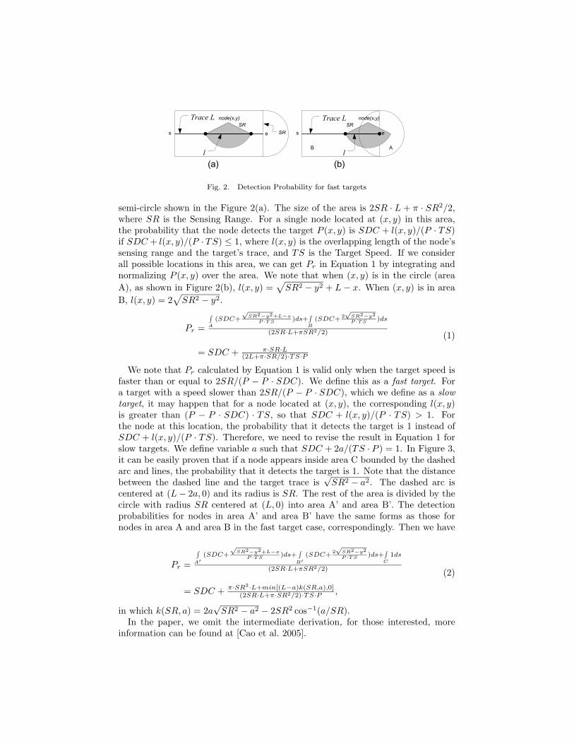
In our VigilNet design, all sentry nodes agree on a common sentry toggle period Pand a common sentry duty cycle SDC. The starting time of a period is randomizedin each node. For each period, a sentry wakes up and stays awake for P · SDC,then goes to sleep for P · (1 − SDC). Assuming a target enters the tracking areafrom point s for L meters till it reaches the point e, as shown in Figure 2(a),we first derive Pr, the probability that a single sentry node detects this target.Obviously, the nodes that may detect the target must be in the rectangle or the
��������
��
�
�
�
������� ��������
��
�
�������
��
�
��� ���
� �
Fig. 2. Detection Probability for fast targets
semi-circle shown in the Figure 2(a). The size of the area is 2SR · L + π · SR2/2,where SR is the Sensing Range. For a single node located at (x, y) in this area,the probability that the node detects the target P (x, y) is SDC + l(x, y)/(P · TS)if SDC + l(x, y)/(P · TS) ≤ 1, where l(x, y) is the overlapping length of the node’ssensing range and the target’s trace, and TS is the Target Speed. If we considerall possible locations in this area, we can get Pr in Equation 1 by integrating andnormalizing P (x, y) over the area. We note that when (x, y) is in the circle (area
A), as shown in Figure 2(b), l(x, y) =√
SR2 − y2 + L − x. When (x, y) is in area
B, l(x, y) = 2√
SR2 − y2.
Pr =
∫
A
(SDC+
√SR2
−y2+L−xP ·T S )ds+
∫
B
(SDC+2√
SR2−y2
P ·T S )ds
(2SR·L+πSR2/2)
= SDC + π·SR·L(2L+π·SR/2)·TS·P
(1)
We note that Pr calculated by Equation 1 is valid only when the target speed isfaster than or equal to 2SR/(P − P · SDC). We define this as a fast target. Fora target with a speed slower than 2SR/(P − P · SDC), which we define as a slowtarget, it may happen that for a node located at (x, y), the corresponding l(x, y)is greater than (P − P · SDC) · TS, so that SDC + l(x, y)/(P · TS) > 1. Forthe node at this location, the probability that it detects the target is 1 instead ofSDC + l(x, y)/(P · TS). Therefore, we need to revise the result in Equation 1 forslow targets. We define variable a such that SDC + 2a/(TS · P ) = 1. In Figure 3,it can be easily proven that if a node appears inside area C bounded by the dashedarc and lines, the probability that it detects the target is 1. Note that the distancebetween the dashed line and the target trace is
√SR2 − a2. The dashed arc is
centered at (L − 2a, 0) and its radius is SR. The rest of the area is divided by thecircle with radius SR centered at (L, 0) into area A’ and area B’. The detectionprobabilities for nodes in area A’ and area B’ have the same forms as those fornodes in area A and area B in the fast target case, correspondingly. Then we have
Pr =
∫
A′
(SDC+
√SR2
−y2+L−xP ·T S )ds+
∫
B′
(SDC+2√
SR2−y2
P ·T S )ds+∫
C
1ds
(2SR·L+πSR2/2)
= SDC + π·SR2·L+min[(L−a)k(SR,a),0](2SR·L+π·SR2/2)·TS·P ,
(2)
in which k(SR, a) = 2a√
SR2 − a2 − 2SR2 cos−1(a/SR).In the paper, we omit the intermediate derivation, for those interested, more
information can be found at [Cao et al. 2005].

(0,0) (L,0)
SRSR
SRA’
B’
C
(L-2a,0)
2a
),( 22aaL −− SR
Trace L
Fig. 3. Detection Probability for slower targets
Now we are ready to provide a statistical real-time guarantee for the initialactivation process, i.e., we need to ensure a target is detected before the sub-deadline Dinitial. Equivalently, a target should be detected before it enters forL = TS · Dinitial meters. Obviously, P (Tinitial < Dinitial) equals P (Tinitial · TS <L), where P (Tinitial · TS < L) is the probability that at least one of nodes inthe area (A+B) detects the target. If there are n nodes in the area, the proba-bility that at least one of them detects the target is 1 − (1 − Pr)
n. Suppose thesentry density is Ds and n conforms to a Poisson distribution with parameter λ=(2SR · L + π · SR2/2)Ds, therefore, the probability that the initial activationfinishes before sub-deadline Dinitial is:
P (Tinitial < Dinitial) = P (Tinitial · TS < L) = 1 − e−Pr·λ (3)
Equation 3 identifies a feasible region for us to decide the system parameterssuch as sentry duty cycle (SDC) and sensing range (SR) to ensure the real-timeproperty in Phase A. In addition, we can obtain the expected value of Tinitial fromthe formula E(Tinitial) =
∫ ∞0
(1 − P (Tinitial < t))dt =∫ ∞0
(1 − P (SD < TS · t))dt.According to Equations 1 and 3, we have the expected delay for a target whosespeed is greater than or equal to 2SR/(P − P · SDC):
E(Tinitial) =e−SDC·π·SR2·DS/2
(2SR · SDC · TS + πSR2/P )DS(4)
Similarly, for a target whose speed is lower than 2SR/(P − P · SDC), we have
E(Tinitial) =e−SDC·π·SR2·DS/2[1 − k(SR,a)e−(2SR·SDC·T S·P )(1−SDC)Ds/2
2SR·SDC·TS·P+πSR2+k(SR,a) ]
(2SR · SDC · TS + πSR2/P )DS(5)
One caveat in the analysis needs some attention. Above we derive the expecteddetection delay for a duty cycle based system with random deployment. However,sentry nodes are located more evenly than totally randomly case [He et al. 2004].Fortunately, we can prove that the random deployment case provides a theoreticalupper bound for the sentry-based deployment case. It can be easily proved that iffor all t, P (T1 < t) > P (T2 < t), we must have E(T1) < E(T2). For 0 < Pr < 1,1 − (1 − Pr)
n is a strictly concave function of n. Therefore, E(1 − (1 − Pr)n) ≤
1− (1−Pr)E(n), and the left side of the equation equals the right side if and only if
n is a constant. Given the same E(n), the more scattered the distribution of n is,the smaller the value of E(1−(1−Pr)
n) is. Since the sentry nodes are selected moreuniformly than the random case, P (Tinitial < Dinitial) for the sentry based systemis greater than a totally randomly distributed system, and therefore the expected
0
200
400
600
800
1000
1200
1400
1600
50 55 60 65 70 75 80 85 90 95
Del
ays(
ms)
Sentry Duty Cycle
T_inital
0
200
400
600
800
1000
1200
1400
1600
50 55 60 65 70 75 80 85 90 95
Del
ays(
ms)
Sentry Duty Cycle
T_inital
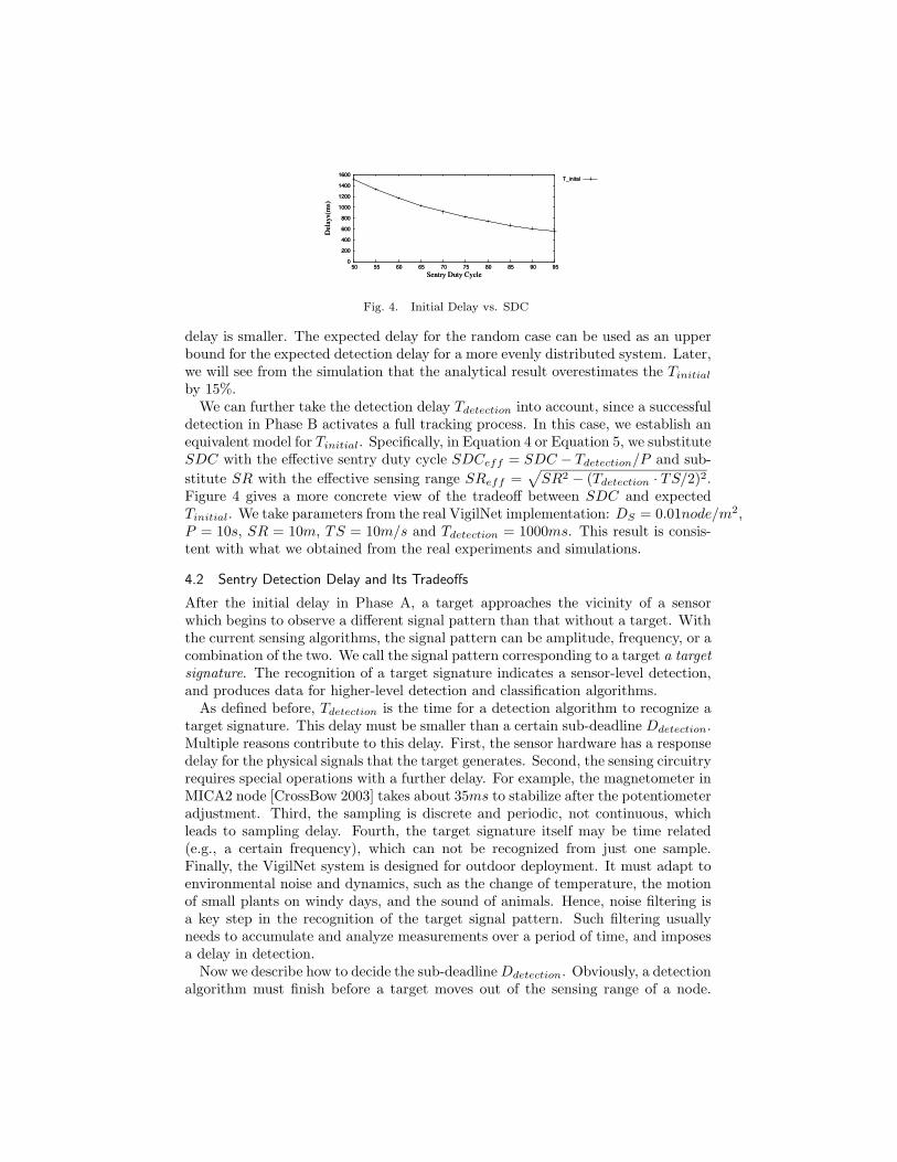
Fig. 4. Initial Delay vs. SDC
delay is smaller. The expected delay for the random case can be used as an upperbound for the expected detection delay for a more evenly distributed system. Later,we will see from the simulation that the analytical result overestimates the Tinitial
by 15%.We can further take the detection delay Tdetection into account, since a successful
detection in Phase B activates a full tracking process. In this case, we establish anequivalent model for Tinitial. Specifically, in Equation 4 or Equation 5, we substituteSDC with the effective sentry duty cycle SDCeff = SDC − Tdetection/P and sub-
stitute SR with the effective sensing range SReff =√
SR2 − (Tdetection · TS/2)2.Figure 4 gives a more concrete view of the tradeoff between SDC and expectedTinitial. We take parameters from the real VigilNet implementation: DS = 0.01node/m2,P = 10s, SR = 10m, TS = 10m/s and Tdetection = 1000ms. This result is consis-tent with what we obtained from the real experiments and simulations.
4.2 Sentry Detection Delay and Its Tradeoffs
After the initial delay in Phase A, a target approaches the vicinity of a sensorwhich begins to observe a different signal pattern than that without a target. Withthe current sensing algorithms, the signal pattern can be amplitude, frequency, or acombination of the two. We call the signal pattern corresponding to a target a targetsignature. The recognition of a target signature indicates a sensor-level detection,and produces data for higher-level detection and classification algorithms.
As defined before, Tdetection is the time for a detection algorithm to recognize atarget signature. This delay must be smaller than a certain sub-deadline Ddetection.Multiple reasons contribute to this delay. First, the sensor hardware has a responsedelay for the physical signals that the target generates. Second, the sensing circuitryrequires special operations with a further delay. For example, the magnetometer inMICA2 node [CrossBow 2003] takes about 35ms to stabilize after the potentiometeradjustment. Third, the sampling is discrete and periodic, not continuous, whichleads to sampling delay. Fourth, the target signature itself may be time related(e.g., a certain frequency), which can not be recognized from just one sample.Finally, the VigilNet system is designed for outdoor deployment. It must adapt toenvironmental noise and dynamics, such as the change of temperature, the motionof small plants on windy days, and the sound of animals. Hence, noise filtering isa key step in the recognition of the target signal pattern. Such filtering usuallyneeds to accumulate and analyze measurements over a period of time, and imposesa delay in detection.
Now we describe how to decide the sub-deadline Ddetection. Obviously, a detectionalgorithm must finish before a target moves out of the sensing range of a node.

Suppose that the nominal sensing area is a circle with a fix sensing range SR, theamount of time a target stays in a node’s sensing range can be derived from thespeed of the target, TS, and the minimum distance from the target’s trajectoryline to the sensor node. Since the target trajectory intersects with the sensingcircle randomly, we assume this minimum distance is uniformly distributed within[0, R), therefore the probability that a target stays in one sensing circle for at leastDdetection seconds can be calculated as
P (t > Ddetection) =
√
1 − (T S·Ddetection)2
4SR2 Ddetection < 2SRT S
P (t > Ddetection) = 0 Ddetection ≥ 2SRT S
(6)
According to Equation 6, the sub-deadline Ddetection can be decided by choosinga desired P (t > Ddetection) value.
0
10
20
30
40
50
60
70
80
90
100
0 0.5 1 1.5 2 2.5 3 3.5
Det
ecti
on c
onfi
den
ce (
per
cent)
Detection delay (second)
Detection confidenceP(x) order 3P(x) order 4P(x) order 5P(x) order 6P(x) order 7P(x) order 8
Fig. 5. Detection Confidence vs. Detection Delay
In addition, we desire to know how a detection algorithm performs under a givensub-deadline Ddetection. We define the Detection Confidence (DC), as the confidenceon the target detection, i.e., 100% DC indicates this sensor has no doubt about theexistence of the target. Normally, the longer Ddetection is, the more informationabout target signature a sensing algorithm can obtain, and therefore, it can achievea higher detection confidence DC. Such a relationship depends on the type ofsensors. In order to quantitatively analyze the relation between DC and Ddetection
as a case study, we performed experiments on XSM motes with the magnetic sensingalgorithm detecting a moving vehicle in an outdoor environment. We approximatethe sensing range as 7 meters around the sensor node, according to empirical data.Figure 5 plots the relation between the detection confidence and the detection delay,based on the experiments. As we can see from the figure, DC does not have a linearrelation to Ddetection. Based on experimental measurements, we use a polynomialto characterize DC versus Ddetection. Figure 5 shows a series of polynomials ofdifferent orders that fit the points representing the relation between the detectionconfidence and the detection delay. The plotting indicates that the polynomials ofan order higher than 5 are fairly close to each other and fit the points well. Hence,

we choose the polynomial of order 5 to characterize the relation, as shown below.
DC = f(Ddetection) =
5∑
i=0
aiDidetection (7)
The coefficients of the polynomial calculated from the curve fitting are a5 =1.0999, a4 = −13.1138, a3 = 51.3443, a2 = −73.2343, a1 = 54.6671, a0 = 0.2402.The polynomial f(Ddetection) characterizes the relation of the detection confidenceand the imposed sub-deadline Ddetection when the vehicle is moving at a relativelylow speed. In the scenarios where the vehicles move faster, the detection delay tendsto be shorter and detection confidence will be higher because the targets impose afaster change to the sensor readings. Hence, f(Ddetection) represents a conservativeestimation of the detection confidence, given a certain amount of time available tothe sensor node to capture and process the target signals.
We note that in the analysis of the time-related properties of the sensing algo-rithms, we choose such a conservative-case approach instead of a worst-case ap-proach. In many cases, the worst-case scenario is a rare event that the system isnot designed to handle well. For example, with the magnetic sensing algorithm,the worst case of detection delay is infinity – if a vehicle moves extremely slowly,it provides a low-frequency signal just as the background noise, resulting in a non-detection for that target. We note that an analysis with such a worst-case scenarioprovides little insight into the system. To represent a reasonably practical scenario,we study a conservative case in which a target can be detected.
In conclusion, we must provide a detection algorithm that finishes before a givensub-deadline Ddetection. According to Equations 6 and 7, when running a detectionalgorithm with a sub-deadline Ddetection, one node can detect P (t > Ddetection)percent of targets with DC percent of the confidence in detection. This analysisjustifies the benefits of fast detection algorithms and the need for group aggregationto improve the detection confidence.
4.3 Wake-up Delay and Its Tradeoff
Once a target is detected in Phase B, we need more nodes to join in order to increasethe confidence in detection. We design a wake-up service to activate the non-sentrynodes after the sentry nodes detect the incoming targets. Different target speedsimpose different sub-deadlines Dwakeup to the wake-up services.
Normally the wake-up service can be supported either through hardware or soft-ware. Several hardware solutions have been proposed in [Dutta et al. 2005; Guand Stankovic 2004]. Since the wake-up circuits accumulate the ambient energyslowly, the current hardware solutions are not fast enough for the real-time targettracking. Therefore, we propose a software-based wake-up strategy, which has ashort average delay and a predictable worse-case delay.
The wake-up operation goes as shown in Figure 6. A non-sentry actually does notsleep all the time. It periodically wakes itself up, quickly senses the radio activity ata particular frequency. If no radio activity is detected, this node goes back to sleep,otherwise it remains active and starts to sample the environment. We control thenon-sentry operation through two parameters: Toggle Period (TP ) and ChannelClear Access duration (CCA). The toggle period is defined as the time interval

) * + ,- . / + / + 0 1 23 45 6 7 8 9 : 9 7 ; 7
: <1 1 / + ) + * = < >
? @A A B CD E FG AH B ? @A A B ? @A A B CD E FG A H B ? @A A B6 <0 I 4+ 0 2 *JK L + *, 2 = < 0
4 + 0 2 *JK L + * , 2 = < 0
Fig. 6. The Wake-up Operation
between two consecutive wake-up instances. The CCA is defined as the minimaltime for a radio module to detect the existence of the radio signal. For example,the CC2420 radio transceiver takes at least 2ms (8 symbol periods, as specified by802.15.4 [IEEE ]) to access the radio activity. Based on TP and CCA, we can getthe Non-Sentry Duty Cycle (NSDC) as CCA
TP . At the sentry side, once a sentrydetects a target, it broadcasts a radio message with a long preamble. This longpreamble is guaranteed to be sensed by neighboring non-sentry nodes as long asthis preamble has a length equal to or longer than the toggle period of non-sentrynodes. The worst case wake-up delay WCDelay equals TP . In other words, the sub-deadline Dwakeup can be ensured trivially in our design by setting TP = Dwakeup.Let the power consumption for an active node during a unit of time be E, theenergy consumption for a non-sentry node is E×CCA
TP . Since the amount of time tocheck the radio activity (CCA) is constant for a specific radio hardware, the lengthof the toggle period determines the energy consumption rate in non-sentry nodes.In general, a long toggle period TP leads to a low energy consumption, however,it also leads to a long delay in waking up the non-sentry nodes. Figure 7 showssuch a tradeoff, using the CC1000 radio transceiver for MICA2/XSM motes as anexample. As shown in Figure 7, a sub-deadline of 200ms lead to a 99% energysaving for the non-sentry nodes.
0 10 20 30 40 50 60 70 80 90 10010
−2
10−1
100
101
102
Energy Conservation Percentage (%)
Wa
ke
up
De
lay (
ms)
Worse Case
Average Case
Fig. 7. Wakeup Delay Vs. Non-Sentry Energy Saving

4.4 Aggregation Delay and Its Tradeoffs
Once all nodes near the target are awakened in Phase C, the group-based trackingbegins. To avoid an excessive power consumption, instead of relaying every detec-tion message back, VigilNet sends only aggregates to the base stations for furtherprocessing. Such an online aggregation process is subject to a certain sub-deadlineDaggregation determined by the target speed and the node density.
Specifically, we organize the nodes in the vicinity of a target into one group.We use a semi-dynamic leader election [Luo et al. 2005] to minimize the delay.Nodes that detect the target become the group members, which, upon detection,immediately report their own locations and sensing data to a leader. The leaderthen averages the locations of members as the estimates of the target positions,and sends such estimates to a base station. To filter out the sporadic false alarmsof individual nodes, we introduce a configurable parameter, DOA (Degree of Ag-gregation), which forces the leader to withhold reports to a base station until thenumber of received member reports reaches DOA. To achieve a high confidence intarget detection, one should set a high DOA value (e.g., 4). On the other hand,a higher DOA value inevitably introduces a longer group aggregation delay sincethe leader waits longer to expect more member reports. This tradeoff allows us tochoose appropriate DOA to meet the sub-deadline Daggregation.
������������
������ ������
Fig. 8. The Detection Areas Before and After Movement
The relation between DOA and the group aggregation delay is complicated byvarious factors, e.g., the sensing range, the target speed, and the node density.Therefore, we make several assumptions to simplify the analysis, including a circularsensing range, a straight target trajectory and randomly distributed nodes. Basedon these assumptions, Figure 8 depicts the movement of a target with a speed TSfor a time period T . Again, the sensing range of a sensor node is SR. The whitecircle and the grey circle denote the detection area of the target before and aftermovement, respectively. Nodes located in the diagonally lined area are the newdetectors of the target, which contribute to DOA by sending reports to the leader.To guarantee a certain sub-deadline Daggregation, the number of new detectors mustexceed or equal DOA before the sub-deadline Daggregation:
Daggregation ≥ Taggregation =DOA
2 · SR · TS · D(8)

where D represents the node density. Note that after the wake-up process, notonly the sentry nodes but also the non-sentry nodes participate in the tracking.Equation 8 quantitatively reveals a feasible region for us to guarantee the sub-deadline Daggregation. For example, if the network density (D) and the sensingrange (SR) are fixed, we can exploit a feasible solution, using different DOA valuesunder different target speeds. Figure 9 gives a more concrete design space bydepicting the group aggregation delay for varied DOA values and target speedswhen the sensing range is 10m, the node density is 1 per 100 m2. We note thatthis result is consistent with the results obtained from the large-scale simulationspresented in Section 7.
0
1
2
3
4
5
1 1.5 2 2.5 3 3.5 4 4.5 5
Del
ays(
ms)
Degree of Aggregation
SPEED=5SPEED=10SPEED=15SPEED=20SPEED=25
0
1
2
3
4
5
1 1.5 2 2.5 3 3.5 4 4.5 5
Del
ays(
ms)
Degree of Aggregation
SPEED=5SPEED=10SPEED=15SPEED=20SPEED=25
Fig. 9. Minimal Group Aggregation Delay for Varying DOA and Target Speed
4.5 Communication Delay and Its Tradeoff
After group aggregation in Phase D, the leader delivers the aggregated trackingreports to a nearby base. Suppose the end-to-end communication sub-deadline isDe2e and one-hop worst case communication delay is TWC MAC [He et al. 2003],we need to ensure that the number of hops is smaller than De2e/TWC MAC . Fora given node density, the hop length Lhop can be estimated through Kleinrock-Silvester formula [L.Kleinrock and J.Slivester 1978], which gives the correlationbetween the hop length Lhop, the communication range CR and the number ofneighbors N as:
Lhop = CR × (1 + e−N −
∫ 1
−1
e−
Nπ
(arccos(t)−t√
1−t2)dt) (9)
Therefore, to guarantee a sub-deadline De2e, when we deploy the network, weshould ensure that every node can reach a base within a radius of Le2e:
Le2e =De2e · Lhop
TWC MAC(10)
In VigilNet, the sub-deadline De2e is guaranteed by partitioning the whole net-work into multiple sections based on the Voronoi diagram [Okabe et al. 2000].Specifically, a network with n bases is partitioned into n Voronoi sections such thateach section contains exactly one base and every node in that Voronoi section iscloser to its base than to any other base inside the network.

4.5.1 Base Deployment Strategy. We have shown that an ideal deployment shouldensure that each node is able to reach a base within a distance of Le2e, so that thesub-deadline De2e can be satisfied. This possesses an implicit requirement on thenumber of base stations and their positions. We therefore provide a detailed analy-sis regarding this requirement and compare the performances of different strategies.
We model the area S with each side as D. Suppose the total number of deployedbase stations is N , each serving nodes located within a radius of L. We assumethat a large number of other non-base nodes are deployed in the area as well. Theproblem is, what is probability that every non-base node can reach a base withina distance of L, given a certain deployment strategy? Furthermore, what is thebest deployment strategy available? We shall analyze three different deploymentstrategies: random, grid and optimal. In particular, we show that the optimalstrategy is a special case of the grid deployment.
We first consider random deployment. We derive the probability in question asfollows. Consider an arbitrary point Q under question. Since each base can servea radius of L, once a base station is deployed, we know that the point Q has a
probability of πL2
S of being located inside this base’s service radius. Therefore,once N bases are deployed, the coverage probability for an arbitrary point Q is
1−(1− πL2
S )N . Notice that this derivation does not take into account the boundaryeffect. This approximation is valid when S � πL2, as verified in our experiment.
0
0.1
0.2
0.3
0.4
0.5
0.6
0.7
0.8
0.9
1
25 50 75 100 125 150 175 200 225 250 275 300
Covera
ge P
robabili
ty
Number of Nodes Deployed
L=50m, Experimental ValueL=75m, Experimental Value
L=100m, Experimental ValueL=125m, Experimental Value
L=50m, Analysis ValueL=75m, Analysis Value
L=100m, Analysis ValueL=125m, Analysis Value
Fig. 10. Random Deployment Performance
Figure 10 validates our analysis on the performance of the random deploymentstrategy. In particular, we assume that D = 1000m. The number of bases N andthe serving distance L are both adjustable. All simulation results are plotted basedon 50 rounds of data, and the confidence interval is 95%. As shown in this figure,the analysis result roughly fits the experimental data, with certain inconsistencies.These inconsistencies are introduced by the boundary effect: the bases deployednear the boundary have a service area less than πL2, therefore, the observed cov-erage probability is slightly lower than the predicted coverage probability.
An interesting problem regarding deployment strategies is redundancy. Sincetypically more bases than needed are provided, it is interesting to consider the

ratio between the number of base stations deployed to the minimum number of basestations required. For example, when L = 100m, using the random deployment,we observe that roughly 150 bases are needed to provide each potential node real-time service (the coverage probability is more than 98%). The redundancy can
be calculated at πL2×ND2 , which is 4.71. This is indeed quite high. We, therefore,
discuss more efficient deployment strategies, assuming we can position the basestations at desired places accurately.
We focus on two types of grid strategies, square based and hexagon based. Thesestrategies are shown in Figure 11.
�������������
���� �������������
������������� ��
���� �������������
�
�
Fig. 11. Regular Deployment Strategies
In the first type of grid deployment, the base stations form a regular squarestructure. The redundancy can be determined to be about 1.57. The second typeof grid deployment forms the honeycomb structure, where regular hexagons areused. Notice that this figure also shows the Voronoi diagram partitions associatedwith the honeycomb structure. The second grid deployment has a redundancy of2π
3√
3, or approximately 1.208.
Previous literature [Williams 1979] has proved that the optimal redundancy ratiofor any circle covering is exactly 2π
3√
3. This result indicates that the honeycomb
based node deployment is the optimal strategy. Indeed, boundary effect also existsin this type of deployment, however, when the area is considerably large, the actualredundancy ratio should approach the optimal bound.
4.6 Base Processing Delay and Its Tradeoffs
After a base receives the reports delivered in phase E, it performs the high-levelprocessing such as the velocity estimation. In order to do so, a base node needsto accumulate several reports from the network. The delay to accumulate thereports Tbase is subject to its sub-deadline Dbase. We defined the minimal numberof reports needed by the base as K. This value can be one, if the in-networkingprocessing is sufficient. The frequency of reports depends on the speed of thetarget and the aggregation of locations from nodes at different locations. From theanalysis in Section 4, we know that after the target enters the system for time t, theexpected number of nodes that can sense the target is (π · SR2/2 + 2SR · TS · t)D.
Obviously, if the target goes further for ∆t, the expected number is increased by2SR · TS · ∆t. Considering the detection delay Tdetection, only nodes that are√
SR2 − (Tdetection · TS/2)2 meters away from the target trajectory can recognizethe target. Therefore, we can estimate the number of reports (NR) generated beforethe sub-deadline Dbase as:
NR = (2TS · D ·√
SR2 − (Tdetection · TS/2)2) · Dbase (11)
Alteratively, to guarantee Dbase, we need to select K, the minimal number ofreports needed by the base, to be a value smaller than NR.
Now we consider how the selection of K impacts the accuracy in velocity estima-tion. Since each location report is an approximation of the target location, there isan error in the result of velocity estimated using the least square method. With-out loss of generality, we first consider the velocity along the x-axis. Statistics hasestablished the variance of the estimated slope in a two-variable least square linearregression as:
σ2
∑Ki=1(xi − x̄2)
,
where σ is the standard deviation of the disturbance, which in our case is thedetection error of a single report; xi in our case is a timestamp. It is hard to getthe distribution of
∑Ki=1(xi − x̄)2, but a rough estimation can be obtained by a
simplification so that the values of xi are evenly distributed and xi = i/(2D · SR ·TS · PR). Thus we can get an estimation of the standard deviation of the velocity:
4σ · D · SR · TS · PR√
3K(K + 1)(K − 1), (12)
where σ is the standard deviation of the location error of a single report. Equa-tion 12 reveals the tradeoff between the accuracy in tracking and the delay in baseprocessing. In brief, Tbase increases linearly with the number of reports requiredand the standard deviation of the velocity estimation reduces approximately lin-early with K−3/2.
4.7 Summary of the Analysis and Tradeoffs
Dealing with the physical world, many sensor-based systems must respond to exter-nal stimuli within certain time constraints. Such constraints could change over timewith the changes of the application objectives. For example, a surveillance systemshould be able to track fast vehicles at a high energy budget as well as slow person-nel at a smaller budget. So it is desirable for a system designer to have the abilityto trade off the system parameters to satisfy certain real-time constraints. In thissection, we use the deadline partition method to guarantee the sub-deadline of eachphase, consequently guaranteeing the end-to-end deadline. This approach makesthe real-time design for a complex sensor network manageable. Since VigilNet aimsat various tracking scenarios, for a given end-to-end deadline, the actually parti-tion among the phases would vary significantly. Our analysis is independent of howthe sub-deadlines are assigned, which gives the designer more flexibility to choose

appropriate partition. Currently, the deadline partition is done statically, and weshall investigate the solutions that allow dynamic online partition in the future.
We note our analysis provides a set of generic design guidelines for other track-ing systems with or without certain features. For example, the tracking systempresented in [Arora et al. 2004] does not consider the power management, whichmakes the analytical results of Tinitial and Twakeup trivially zero, while other an-alytical results are still applicable. Other notable insights from our analysis are:First, to guarantee the same sub-deadline, a higher node density is desired in theslow-target case, however a slower duty cycle can be tolerated without jeopardizingthe detection. Second, it is very beneficial to increase the wake-up delay, whenpossible, in exchange for the energy saving. Third, fast detection algorithms are es-sential. Fourth, a low network density increases the group aggregation delay, whichindirectly reduces the detection confidence. Fifth, theoretically, honeycomb is theoptimal base placement strategy.
We also note due to the unpredictable and statistical nature of environmentalinputs (e.g., a target could move infinitely slowly, and sensing and communicationranges could be highly irregular), VigilNet is not quite amenable to the traditionalprecise worst-case real-time analysis. Nevertheless, the analytical results we providecan assist the designer to provide soft real-time guarantee and make guided decisionson system configurations. In the Section 6 and Section 7, we validate our real-timedesign and analysis through a physical test-bed with 200 XSM motes as well as alarge-scale simulator with 10,000 nodes, respectively.
5. SYSTEM IMPLEMENTATION
A large portion of code of VigilNet is written in NesC [Gay et al. 2000], a moduleoriented extension of the C programming language. Since the concept of traditionalOS kernels does not exist in TinyOS [Hill et al. 2000], a NesC programmer candirectly access the hardware devices, which facilitates the time analysis within asingle node [Mohan et al. 2004]. The network infrastructure in VigilNet is a multi-path diffusion tree rooted at bases. The contention-based B-MAC protocol [Polastreand Culler 2004] is the default media access control protocol, which has certainuncertainty in the communication delay. Three detection algorithms are designedseparately for acoustic, magnetic and motion sensors. They identify the targetsignatures through a lightweight classification scheme as described in [Gu et al.2005]. VigilNet consists 40,000 lines of code, supporting multiple existing moteplatforms including MICA2, MICA2dot and XSM. The compiled image occupies83,963 bytes of code memory and 3,586 bytes of data memory.
Among 30 protocols implemented within VigilNet, we only describe the time-related services here. Other information can be found at [He et al. 2006; He et al.2006; He et al. 2004]. VigilNet needs a millisecond-level synchronization to co-ordinate the operations among the nodes. In addition, to obtain precise timingmeasurements in the experiments, we need a network-wide synchronization be-tween a base and other nodes within the field. Several well-known schemes areable to achieve a high synchronization precision, however they do not match wellwith VigilNet requirements. GPS-based schemes [Wellenhoff et al. 1997] typicallyachieve persistent synchronization with a precision of about 200 ns. However, GPS

devices are expensive and bulky. The reference broadcast scheme (RBS) proposedin [Elson and Romer 2002] maintains information relating the phase and frequencyof each pair of clocks in the neighborhood of a node. While RBS achieves a precisionof about 1 µs, the message overhead in maintaining the neighborhood information ishigh and may not be energy-efficient in large systems. We believe that fine-grainedclock synchronization achieved by costly periodic beacon exchanges may not besuitable for the energy-constrained surveillance system. Therefore, we modifiedthe FTSP time synchronization protocol [Maroti et al. 2004] to synchronize themotes only during the initialization phase, using a synchronization beacon broad-cast by the base station at the beginning of each initialization cycle. Since theunderlying MAC layer provided by TinyOS does not guarantee reliable delivery,the base station retransmits the synchronization beacon multiple times. The syn-chronization beacons are propagated across the network through limited floodingwith timestamp values reassigned at intermediate motes immediately prior to thetransmission of the timestamp. This eliminates the uncertainty in MAC contentiondelay. Receivers take the timestamp from the beacon plus a fixed hardware delayas their own local time. The timer drift that accumulates over time is rectifiedby a new system cycle (i.e., a repeated initialization phase). The frequency of re-initialization is a configurable parameter, which can be calculated based on the rateof clock drift and the desired accuracy of time synchronization. As for the currentVigilNet system, the accuracy of tens of milliseconds is sufficient, which leads toabout once per day synchronization.
6. EVALUATION OF REAL SYSTEM PERFORMANCE
In the evaluation, we validate the analytical results as well as provide more insightsinto the timing issues from the real system and simulation perspectives.
6.1 Experimental Settings
Fig. 12. Deployment Site
As a real-time online tracking system, VigilNet is designed to complete detection,classification and velocity estimation within 4 seconds. The field test was done

on a T-shape dirt road in Florida as shown in Figure 12 from the aerial view.We deployed 200 XSM motes which are equipped with CC1000 radio, magnetic,acoustic, photo, temperature and passive infrared sensors (PIR). Along the road,nodes were randomly placed roughly 10 meters apart, covering one 300-meter roadand one 200-meter road. Through a certain localization [Stoleru et al. 2004; Heet al. 2003; Stoleru et al. 2005], nodes were aware of their positions. In order tomeasure various kinds of delay, all nodes within VigilNet synchronized with the basewithin 1∼10 milliseconds using the techniques described in [Maroti et al. 2004]. Thetime stamps of various actions such as initial detection were sent back to the base,so that we can calculate the delay. We used a Ford Explorer that weighted about4000 lbs. as the target.
6.2 Delay Measurements
When a car enters the surveillance area at about 10 meters per second (22 mph),a detection report is issued first, followed by classification reports. Finally, aftersufficient information is gathered, velocity reports are issued. Figure 13 illustratesthe cumulative distribution of different delays. The communication delay (leftmostcurve) is much smaller compared with other delays. About 80% of detections aredone within 2 seconds. Over 80% of the classification and velocity estimations aremade within 4 seconds. The empirical results from most runs are consistent withour analysis in Section 4 and the simulation results in Section 7.
0%
20%
40%
60%
80%
100%
0 1000 2000 3000 4000 5000 6000 7000 8000 9000
Delay (ms)
Cu
mu
lati
ve
Dis
trib
uti
on
of
De
lay
s
T_initial
T_initial+T_decetion+T_agg+T_e2e
T_total
T_e2e
Fig. 13. Various Delays Measurements from Field Test
We emphasize here that field experiments indicate that VigilNet meets its real-time requirement and our real-time analysis can approach the reality with a reason-able precision, despite the amount of complexity within the VigilNet (30 protocolsintegrated). On the other hand, we acknowledge that due to various physical con-straints, field experiments can only exploit a very limited design space and obtaina limited amount of data. Therefore, to understand the real-time properties inVigilNet at scale with a much larger context, we provide a large-scale simulation inthe next section.
7. LARGE-SCALE SIMULATION
Our simulator is a discrete simulator, written in C++. It emulates the trackingoperations as shown in Figure 1. We distribute 10,000 nodes randomly within a100,000 m2 rectangle area, assuming nominal circular sensing and communication

ranges. We run each experiment 30 times with different random numbers. Thefigures are plotted with the average value as well as the 95% confidence interval.
7.1 Experiment Setup
We note that our evaluation does not choose deadline/sub-deadline miss ratiosas the major metrics, because such an approach reveals less information about thetradeoff between actual delays and other system performance parameters. Since themean value and 95% confidence intervals of the delays are plotted in the figures, onecan determine the appropriate system settings for a given deadline requirement.
In our experiments, we study several system-wide parameters that directly affectthe real-time properties of VigilNet. These parameters are: 1) the target speed(TS), 2) the physical delay in detection (Tdetection), 3) the sentry duty cycle (SDC),4) the non-sentry duty cycle (NSDC), 5) the required degree of aggregation (DOA),6) the sensing range (SR) and 7) the required number of reports for base processing(K). We match the simulations with the analysis to see how well they fit with eachother.
We use the settings from the VigilNet system as the default values for thesesystem parameters, which are listed in Table I. Unless mentioned otherwise, thedefault values in Table I are used in all experiments. The metrics used to measurethe system performance are mainly the six types of delays discussed in Section 2,the end-to-end delay and the energy consumption per day per node.
Table I. Key System Parameters
Parameter Definition Default ValueTS Target Speed 10 m/sSDC Sentry Duty Cycle 50%NSDC Non-Sentry Duty Cycle 1%DOA Degree of Aggregation 1%SR Sensing Range 10K Reports required by the base 1
D Node Density 0.01 m2
0
500
1000
1500
2000
2500
3000
3500
4 6 8 10 12 14 16 18 20 22 24
Del
ays(
ms)
Target Speed
T_initalT_detection
T_wakeupT_aggT_e2e
T_baseT_total
0
500
1000
1500
2000
2500
3000
3500
4 6 8 10 12 14 16 18 20 22 24
Del
ays(
ms)
Target Speed
T_initalT_detection
T_wakeupT_aggT_e2e
T_baseT_total
Fig. 14. Delays vs. Target Speed

15
15.1
15.2
15.3
15.4
15.5
15.6
4 6 8 10 12 14 16 18 20 22 24
Av
g E
ner
gy
Co
nsu
med
P
er D
ay P
er N
od
e (m
Ah
)
Target Speed
Energy Consumption Per Day 15
15.1
15.2
15.3
15.4
15.5
15.6
4 6 8 10 12 14 16 18 20 22 24
Av
g E
ner
gy
Co
nsu
med
P
er D
ay P
er N
od
e (m
Ah
)
Target Speed
Energy Consumption Per Day
Fig. 15. Energy Consumption vs. Target Speed
7.2 Performance vs. Target Speed
The target speed determines the spatiotemporal distribution of events over a certaintime period. It is crucial to understand its impacts on the tracking performance.In this experiment, we incrementally increase the target speed (TS) from 5m/s to15m/s in steps of 1 meter. As expected from our analysis in Section 4, Tinitial andTaggregation decrease with the target speed, as shown in Figure 14. One interestingobservation is that the descend rate of Tinitial diminishes when TS becomes larger.This is because a node needs a sufficient sensing time to ensure detection. It ispossible that a quick target passes one sensor without detection, which negativelyaffects the Tinitial. Since VigilNet deals with a rare event model, the energy con-sumed during the tracking is not perceptibly affected by the target speeds as shownin Figure 15.
0
500
1000
1500
2000
2500
3000
3500
500 550 600 650 700 750 800 850 900 950
Del
ays(
ms)
Detection Delay
T_initalT_detection
T_wakeupT_aggT_e2e
T_baseT_total
0
500
1000
1500
2000
2500
3000
3500
500 550 600 650 700 750 800 850 900 950
Del
ays(
ms)
Detection Delay
T_initalT_detection
T_wakeupT_aggT_e2e
T_baseT_total
Fig. 16. Delays under Varying Detection Delay
7.3 Performance vs. Detection Delay
Different tracking systems use different sensing devices and detection algorithms,which have various detection delays Tdetection. In this experiment, we increase thedelay in the detection algorithm Tdetection from 500 ms to 1000 ms in steps of 50 ms.It is interesting to observe in Figure 16 that at a speed of 10m/s, the detection delayhas a small impact on the initial delay, however it contributes most significantly tothe overall increase of the total tracking delay. Again, since the detection time isrelatively small, this system parameter does not noticeably affect the overall energyconsumption, as shown in Figure 17.

15
15.1
15.2
15.3
15.4
15.5
15.6
500 550 600 650 700 750 800 850 900 950
Avg E
ner
gy C
onsu
med
P
er D
ay P
er N
ode
(mA
h)
Detection Delay
Energy Consumption Per Day 15
15.1
15.2
15.3
15.4
15.5
15.6
500 550 600 650 700 750 800 850 900 950
Avg E
ner
gy C
onsu
med
P
er D
ay P
er N
ode
(mA
h)
Detection Delay
Energy Consumption Per Day
Fig. 17. Energy Consumption vs. Detection Delay
0
500
1000
1500
2000
2500
3000
50 55 60 65 70 75 80 85 90 95
Del
ays(
ms)
Sentry Duty Cycle
T_initalT_detection
T_wakeupT_aggT_e2e
T_baseT_total
0
500
1000
1500
2000
2500
3000
50 55 60 65 70 75 80 85 90 95
Del
ays(
ms)
Sentry Duty Cycle
T_initalT_detection
T_wakeupT_aggT_e2e
T_baseT_total
Fig. 18. Delays vs. Sentry Duty Cycle
16
18
20
22
24
26
28
30
50 55 60 65 70 75 80 85 90 95
Av
g E
ner
gy
Co
nsu
med
P
er D
ay P
er N
od
e (m
Ah
)
Sentry Duty Cycle
Energy Consumption Per Day 16
18
20
22
24
26
28
30
50 55 60 65 70 75 80 85 90 95
Av
g E
ner
gy
Co
nsu
med
P
er D
ay P
er N
od
e (m
Ah
)
Sentry Duty Cycle
Energy Consumption Per Day
Fig. 19. Energy Consumption vs. Sentry Duty Cycle
7.4 Performance vs. Sentry Duty Cycle
From the analytical results in Section 4, we obtain an analytical delay curve betweenTinitial and SDC in Figure 4. In this experiment, we obtain a set of other curves(Figure 18) through the simulation. By comparing these two results, we concludethat they are consistent with each other. For example, at a default 50% duty cycle,Tinitial obtained from the analysis in Figure 4 is 1600ms, while Tinitial obtainedfrom the simulation (Figure 18) is 1360ms (Note that our analysis is relativelyconservative). In addition, Figure 19 reveals that the energy consumption escalateslinearly with the SDC, which indicates that an efficient sentry scheduling algorithmis beneficial.

0
500
1000
1500
2000
2500
3000
1 2 3 4 5 6 7 8 9 10
Del
ays(
ms)
Non-Sentry Duty Cycle
T_initalT_detection
T_wakeupT_aggT_e2e
T_baseT_total
0
500
1000
1500
2000
2500
3000
1 2 3 4 5 6 7 8 9 10
Del
ays(
ms)
Non-Sentry Duty Cycle
T_initalT_detection
T_wakeupT_aggT_e2e
T_baseT_total
Fig. 20. Delays vs. Non-Sentry Duty Cycle
15
15.5
16
16.5
17
17.5
18
18.5
19
19.5
20
1 2 3 4 5 6 7 8 9 10
Av
g E
ner
gy
Co
nsu
med
P
er D
ay P
er N
od
e (m
Ah
)
Non-Sentry Duty Cycle
Energy Consumption Per Day 15
15.5
16
16.5
17
17.5
18
18.5
19
19.5
20
1 2 3 4 5 6 7 8 9 10
Av
g E
ner
gy
Co
nsu
med
P
er D
ay P
er N
od
e (m
Ah
)
Non-Sentry Duty Cycle
Energy Consumption Per Day
Fig. 21. Energy Consumption vs. Non-Sentry Duty Cycle
7.5 Performance vs. Non-sentry Duty cycle
Here, we evaluate the impact of the wake-up operation on the delay and energyconsumption. First, the simulation results confirm that the average wake-up delayis approximately half of the toggle period as predicted in Section 4.3. Since thewake-up delay Twakeup is one order of magnitude smaller than other delays suchas Tinitial, a slight decrease in the wake-up delay, shown in Figure 20, does notnoticeably impact the overall delay. However, interestingly a slight increase of theNon-Sentry Duty Cycle leads to a significant increase in energy consumption asshown in Figure 21. This is because the non-sentry nodes are by far the majority,so a duty-cycle increase for the non-sentry nodes leads to a quick increase in thetotal energy. This result indicates that it is beneficial to increase the wake-up delay,when possible, in exchange for the energy saving.
0
1000
2000
3000
4000
5000
6000
1 1.5 2 2.5 3 3.5 4 4.5 5
Del
ays(
ms)
Degree of Aggregation
T_initalT_detection
T_wakeupT_aggT_e2e
T_baseT_total
0
1000
2000
3000
4000
5000
6000
1 1.5 2 2.5 3 3.5 4 4.5 5
Del
ays(
ms)
Degree of Aggregation
T_initalT_detection
T_wakeupT_aggT_e2e
T_baseT_total
Fig. 22. Delays vs. DOA

15
15.1
15.2
15.3
15.4
15.5
15.6
1 1.5 2 2.5 3 3.5 4 4.5 5
Av
g E
ner
gy
Co
nsu
med
P
er D
ay P
er N
od
e (m
Ah
)
Degree of Aggregation
Energy Consumption Per Day 15
15.1
15.2
15.3
15.4
15.5
15.6
1 1.5 2 2.5 3 3.5 4 4.5 5
Av
g E
ner
gy
Co
nsu
med
P
er D
ay P
er N
od
e (m
Ah
)
Degree of Aggregation
Energy Consumption Per Day
Fig. 23. Energy Consumption vs. DOA
7.6 Performance vs. DOA
In-network processing through data aggregation can reduce the amount of datatransmitted over the network and can increase the confidence in target detection.However, to accumulate enough report, it inevitably introduces a certain delay.This experiment studies the effects of data aggregation. We gradually increase theDOA threshold for a leader to report to the base. Since the DOA value only affectsthe tracking phase, which has a small energy consumption, DOA’s impact on theenergy consumption is not noticeable. On the other hand, with a larger DOA value,it takes more time for a leader to collect the member reports. For example as shownin Figure 22, it takes as long as 2.39 seconds to achieve DOA value of 5. We notethat this simulation result is again consistent with the analytical results shown inFigure 9, which has an estimated delay of 2.5 seconds.
0
500
1000
1500
2000
2500
3000
10 12 14 16 18 20 22 24 26 28
Del
ays(
ms)
Sensing Range
T_initalT_detection
T_wakeupT_aggT_e2e
T_baseT_total
0
500
1000
1500
2000
2500
3000
10 12 14 16 18 20 22 24 26 28
Del
ays(
ms)
Sensing Range
T_initalT_detection
T_wakeupT_aggT_e2e
T_baseT_total
Fig. 24. Delays vs. Sensing Range
7.7 Performance vs. Sensing Range
To accommodate various requirements in detection and classification, differenttracking systems use sensors with different ranges. Figure 24 and Figure 25 in-vestigate the impact of sensing range to the tracking performance and energy con-sumption. With a large sensing range, a smaller number of sentries is required.Therefore, the total energy consumption decreases quickly. For example in Fig-ure 25, the energy reduces by 75% when the sensing range increases from 10m to28m. It is interesting to see that the initial delay Tinitial actually slightly increases.This is because the number of sentry nodes reduces while the coverage per sensor

0
2
4
6
8
10
12
14
16
10 12 14 16 18 20 22 24 26 28
Av
g E
ner
gy
Co
nsu
med
P
er D
ay P
er N
od
e (m
Ah
)
Sensing Range
Energy Consumption Per Day 0
2
4
6
8
10
12
14
16
10 12 14 16 18 20 22 24 26 28
Av
g E
ner
gy
Co
nsu
med
P
er D
ay P
er N
od
e (m
Ah
)
Sensing Range
Energy Consumption Per Day
Fig. 25. Energy Consumption vs. Sensing Range
increases, the total coverage by all sentry nodes remains the same. We can de-rive from Equation 3 that the expected Tinitial is higher when the sensing range issmaller, given the same coverage in both cases. This analytic result is confirmed bythe simulation results shown in Figure 24. Due to the space constraints, we omitthe detailed derivation here.
0
1000
2000
3000
4000
5000
6000
7000
8000
1 2 3 4 5 6 7 8 9 10
Del
ays(
ms)
Number of Reports required by Base
T_initalT_detection
T_wakeupT_aggT_e2e
T_baseT_total
0
1000
2000
3000
4000
5000
6000
7000
8000
1 2 3 4 5 6 7 8 9 10
Del
ays(
ms)
Number of Reports required by Base
T_initalT_detection
T_wakeupT_aggT_e2e
T_baseT_total
Fig. 26. Delays vs. Num of Required Reports
15
15.1
15.2
15.3
15.4
15.5
15.6
1 2 3 4 5 6 7 8 9 10
Av
g E
ner
gy
Co
nsu
med
P
er D
ay P
er N
od
e (m
Ah
)
Number of Reports required by Base
Energy Consumption Per Day 15
15.1
15.2
15.3
15.4
15.5
15.6
1 2 3 4 5 6 7 8 9 10
Av
g E
ner
gy
Co
nsu
med
P
er D
ay P
er N
od
e (m
Ah
)
Number of Reports required by Base
Energy Consumption Per Day
Fig. 27. Energy Consumption vs. Num of Required Report
7.8 Performance vs. Number of Reports
To improve the estimation of target velocity and to classify targets with a highconfidence, a base node normally needs to accumulate a certain number of spa-tiotemporally related reports from the same logic tracking group. This experimentinvestigates the impact of the number of reports required by a base on the tracking

delays. Obviously, this only affects Tbase. Figure 26 shows that Tbase approximatelyincreases linearly with the number of reports, which is expected from our analyticalresults in Section 4.6. Since the operation is done at the base, there is no energyimpact to the sensor network, as shown in Figure 27.
8. RELATED WORK
Real-time protocols have been designed at different layers to guarantee the effec-tiveness of the interactions between wireless sensor networks and the physical world.At the MAC layer, RAP [Lu et al. 2002] uses a novel velocity monotonic schedulingto prioritize the real-time traffic and enforce such prioritization through a differenti-ated MAC Layer. Woo and Culler [Woo and Culler 2001] propose an adaptive ratecontrol scheme to achieve fairness among the nodes with different distances to a basestation. Li [Li et al. 2005] proposes a SLF message scheduling algorithm to exploitspatial channel reuse, so that deadline misses can be reduced. Carley [Carley et al.2003] designs a periodic message scheduler to provide a contention-free predicablemedium access control. At the network layer, He [He et al. 2003]et al. support asoft real-time communication service with a desired delivery speed across the sensornetwork, using feedback-based adaptation algorithms that enforce per-hop speed inface of unpredictable traffic. Felemban [Felemban et al. 2005] presents a novelpacket delivery mechanism, called multi-path and multi-speed routing protocol, forprobabilistic QoS guarantee in wireless sensor networks. At the aggregation layer,Vasudevan [Vasudevan et al. 2003] proposes an application-specific compression fortime delay estimation in sensor networks, and He [He et al. 2004] adaptively per-forms application independent data aggregation in a time sensitive manner. Thereal-time solutions at the application is highly diversified. Huang [Huang et al.2003] et al. propose the Mobicast protocol to provide just-in-time information dis-semination to nodes in a mobile delivery zone. Given the complete knowledge oftraffic pattern, Somasundara [Somasundara et al. 2004] proposes a mobile agentscheduling algorithm to collect the buffered sensor data, before the buffer overflowoccurs at the sensor nodes. Nam [Nam et al. 2005] proposes time-parameterizedsensing task model for real-time tracking. Yang [Yang and Vaidya 2004] proposesa wakeup scheme that assists balancing energy saving and end-to-end delay. TheLightning protocol [Wang et al. 2004] localizes the acoustic source with a boundeddelay regardless of the node density.
Besides the real-time protocol design, several researchers have focused on thetime analysis for sensor networks. Lu [Lu et al. 2005] studies how to minimizethe communication latency given that each sensor has a duty cycling requirementof being awake for only 1
k time slots on average. In [Mohan et al. 2004], Mohanet al. provides a cycle-accurate WCET analysis tool for the applications runningon the Atmega Processor Family. Abdelzaher [Abdelzaher et al. 2004] derives areal-time capacity bound for multi-hop wireless sensor networks. It is a sufficientschedulability condition for a class of fixed priority packet scheduling algorithms.Using this bound, one can determine whether a certain traffic pattern can meet itsreal-time requirement beforehand.
With advances in the sensor techniques, several large-scale sensor systems havebeen built recently. The GDI Project [Szewczyk et al. 2004] provides an environ-

mental monitoring system to record animal behaviors for a long period of time.The shooter localization system [Simon et al. 2004] collects the time-stamps ofthe acoustic detection from different nodes within the network to localize the posi-tions of the snipers. These systems mention some timing issues, however they donot treat real-time as a major concern. Our previous publications on VigilNet [Heet al. 2004; He et al. 2006] focus on the middleware services and overarching systemintegration. To the best of our knowledge, this work is the first to analyze thereal-time performance and its tradeoffs in a real-world large-scale wireless sensorsystem.
9. CONCLUSION
In this paper, we demonstrate the feasibility to design a complex real-time sen-sor network, using the deadline partition method, which guarantees an end-to-endtracking deadline by satisfying a set of sub-deadlines. We also analytically identifythe tradeoffs among system properties while meeting the real-time requirements.We validate our design and analysis through both a large-scale simulation with10,000 nodes as well as a field test with 200 XSM nodes. We contribute a set oftradeoffs that are useful for the future development of real-time sensor systems.Given real-time constraints, a system designer can make guided engineering judg-ments on the system parameters. Here we just name a few. First, to guaranteethe same sub-deadline, a higher node density is desired in the slow-target case,however a slower duty cycle can be tolerated without jeopardizing the detection.Second, it is beneficial to increase the wake-up delay, when possible, in exchangefor the energy saving. Third, fast detection algorithms are essential. Fourth, a lownetwork density increases the group aggregation delay, which indirectly reduces thedetection confidence. Fifth, theoretically, honeycomb is the optimal base placementstrategy to meet the communication sub-deadline.
Finally, we acknowledge that although it is amenable to provide the worst-casereal-time analysis for a certain protocol such as the wake-up protocol in Section 4.3,however, due to the dynamic and unpredictable nature of the sensor networks, itis a long-term research goal for us to achieve precise worst-case real-time analysisacross the whole system.
10. ACKNOWLEDGEMENTS
This work was supported in part by the DAPRPA IXO offices under the NESTproject (grant number F336615-01-C-1905), the MURI award N00014-01-1-0576from ONR, NSF grant CCR-0329609, CCR-0325197 and CNS-0435060. The au-thors specially thank the NEST program manager Dr. Vijay Raghavan for hisvaluable contributions.
REFERENCES
Abdelzaher, T. F., Prabh, S., and Kiran, R. 2004. On Real-Time Capacity Limits of
Multihop Wireless Sensor Networks. In IEEE RTSS.
Arora, A., Dutta, P., Bapat, S., Kulathumani, V., Zhang, H., Naik, V., Mittal, V., Cao,
H., Demirbas, M., Gouda, M., Choi, Y., Herman, T., Kulkarni, S., Arumugam, U.,Nesterenko, M., Vora, A., and Miyashita, M. 2004. A Wireless Sensor Network for
Target Detection, Classification, and Tracking. Computer Networks (Elsevier).

Arora, A. and et al. 2005. Exscal: Elements of an extrem scale wireless sensor network. In
11th IEEE International Conference on Embedded and Real-Time Computing Systems and
Applications (RTCSA 2005).
Cao, Q., Yan, T., Abdelzaher, T., and Stankovic, J. 2005. Analysis of target detection
performance for wireless sensor networks. In DCOSS’05.
Carley, T. W., Ba, M. A., Barua, R., and Stewart, D. B. 2003. Contention-free periodic
message scheduler medium access control in wireless sensor/actuator networks. In IEEE
RTSS.
CrossBow 2003. Mica2 data sheet. CrossBow. Available at http://www.xbow.com.
Dutta, P., Grimmer, M., Arora, A., Biby, S., and Culler, D. 2005. Design of a Wireless
Sensor Network Platform for Detecting Rare, Random, and Ephemeral Events. In IPSN’05.
Elson, J. and Romer, K. 2002. Wireless Sensor Networks: A New Regime for Time
Synchronization. In Proc. of the Workshop on Hot Topics in Networks (HotNets).
Felemban, E., Lee, C., Ekici, E., Boder, R., and Vural, S. 2005. Probabilistic qos guarantee
in reliablility and timeliness domains in wireless senosr networks. In IEEE INFOCOM 2005.
Gay, D., Levis, P., von Behren, R., Welsh, M., Brewer, E., and Culler, D. 2000. ThenesC Language: A Holistic Approach to Networked Embedded Systems. In Proceedings ofProgramming Language Design and Implementation (PLDI) 2003.
Gu, L., Jia, D., Vicaire, P., Yan, T., Luo, L., A.Tirumala, Cao, Q., T. He, J. A. S.,
T.Abdelzaher, and Krogh., B. 2005. Lightweight Detection and Classification for WirelessSensor Networks in Realistic Environments. In SenSys’05.
Gu, L. and Stankovic, J. A. 2004. Radio-Triggered Wake-Up Capability for Sensor Networks.In Proceedings of RTAS.
He, T., Blum, B. M., Stankovic, J. A., and Abdelzaher, T. F. 2004. AIDA: AdaptiveApplication Independent Data Aggregation in Wireless Sensor Networks. ACM Transactionson Embedded Computing Systems, Special issue on Dynamically Adaptable Embedded
Systems.
He, T., Huang, C., Blum, B. M., Stankovic, J. A., and Abdelzaher, T. 2003. Range-FreeLocalization Schemes in Large-Scale Sensor Networks. In MOBICOM’03.
He, T., Krishnamurthy, S., Luo, L., Yan, T., Stoleru, R., Zhou, G., Cao, Q., Vicaire, P.,Stankovic, J. A., Abdelzaher, T. F., Hui, J., and Krogh, B. 2006. VigilNet: An
Integrated Sensor Network System for Energy-Efficient Surveillance. ACM Transaction onSensor Networks.
He, T., Krishnamurthy, S., Stankovic, J. A., Abdelzaher, T., Luo, L., Stoleru, R., Yan,
T., Gu, L., Hui, J., and Krogh, B. 2004. An Energy-Efficient Surveillance System Using
Wireless Sensor Networks. In MobiSys’04.
He, T., Stankovic, J., Lu, C., and Abdelzaher, T. 2003. SPEED: A Stateless Protocol for
Real-Time Communication in Ad Hoc Sensor Networks. In ICDCS’03.
He, T., Vicaire, P., Yan, T., Cao, Q., Zhou, G., Gu, L., Luo, L., Stoleru, R., Stankovic,
J. A., , and Abdelzaher, T. 2006. Achieving Long-Term Surveillance in VigilNet. In IEEE
Infocom.
Hill, J., Szewczyk, R., Woo, A., Hollar, S., Culler, D. E., and Pister, K. S. J. 2000.System Architecture Directions for Networked Sensors. In Proc. of Architectural Support for
Programming Languages and Operating Systems (ASPLOS). 93–104.
Huang, Q., Lu, C., and Roman, G.-C. 2003. Spatiotemporal Multicast in Sensor Networks. In
SenSys 2003.
IEEE. IEEE Wireless Medium Access Control(MAC) and Physical Layer (PHY) Specifications
for Low-Rate Wireless Personal Area Networks (LR-WPANs).
Juang, P., Oki, H., Wang, Y., Martonosi, M., Peh, L., and Rubenstein, D. 2002.
Energy-Efficient Computing for Wildlife Tracking: Design Tradeoffs and Early Experiences
with ZebraNet. In Proc. of ASPLOS-X.
Li, H., Shenoy, P., and Ramamritham, K. 2005. Scheduling Messages with Deadlines in
Multi-hop Real-time Sensor Networks. In RTAS’05.

L.Kleinrock and J.Slivester. 1978. Optimum transmission radii for packet radio networks or
why six is a magic number. In national Telecomm conference.
Lu, C., Blum, B. M., Abdelzaher, T. F., Stankovic, J. A., and He, T. 2002. Rap: A
real-time communication architecture for large-scale wireless sensor networks. In IEEE RTAS.
Lu, G., Sadagopan, N., Krishnamachari, B., and Goel, A. 2005. Delay efficient sleep
scheduling in wireless sensor networks. In IEEE INFOCOM 2005.
Luo, L., He, T., Abdelzaher, T., and Stankovic, J. 2005. Design and comparison of
lightweight group management strategies in envirosuite. In DCOSS ’05: International
Conference on Distributed Computing in Sensor Networks.
Maroti, M., Kusy, B., Simon, G., and Ledeczi, A. 2004. The Flooding Time Synchronization
Protocol. In SenSys’04. 39–49.
Mohan, S., Mueller, F., Whalley, D., and Healy, C. 2004. Timing Analysis for Sensor
Network Nodes of the Atmega Processor Family. In IEEE RTSS.
Nam, M.-Y., Lee, C.-G., Kim, K., and Caccamo, M. 2005. Time-parameterized sensing task
model for real-time tracking. In IEEE RTSS 2005.
Okabe, A., Boots, B., Sugihara, K., and Chiu, S. N. 2000. Spatial Tessellations:Concepts
and Applications of Voronoi Diagrams. Wiley.
Polastre, J. and Culler, D. 2004. Versatile Low Power Media Access for Wireless Sensor
Networks. In Second ACM Conference on Embedded Networked Sensor Systems (SenSys2004).
Simon, G., Maroti, M., Ledeczi, A., Balogh, G., Kusy, B., Nadas, A., Pap, G., Sallai, J.,and Frampton, K. 2004. Sensor Network-Based Countersniper System. In SenSys’04.
Somasundara, A. A., Ramamoorthy, A., and Srivastava, M. B. 2004. Mobile ElementScheduling for Efficient Data Collection in Wireless Sensor Networks with DynamicDeadlines. In IEEE RTSS.
Stoleru, R., He, T., and Stankovic, J. A. 2004. Walking GPS: A Practical Solution forLocalization in Manually Deployed Wireless Sensor Networks. In EmNetS-I.
Stoleru, R., He, T., Stankovic, J. A., and Luebke, D. 2005. High-Accuarcy, Low-CostLocalization System for Wireless Sensor Networks. In Third ACM Conference on Embedded
Networked Sensor Systems (SenSys 2005).
Szewczyk, R., Mainwaring, A., Anderson, J., and Culler, D. 2004. An Analysis of a Large
Scale Habit Monitoring Application. In SenSys’04.
Vasudevan, L., Ortega, A., and Mitra, U. 2003. Application-Specific Compression for Time
Delay Estimation in Sensor Netowrks. In ACM SenSys 2003.
Wang, Q., Zheng, R., Tirumal, A., Liu, X., and Sha, L. 2004. Lightning: A Fast andLightweight Acoustic Localization Protocol Using Low-End Wireless Micro-Sensors. In IEEE
RTSS.
Wellenhoff, B. H., Lichtenegger, H., and Collins, J. 1997. Global Positions System:
Theory and Practice,Fourth Edition. Springer Verlag.
Williams, R. 1979. Circle Coverings. In The Geometrical Foundation of Natural Structure: A
Source Book of Design, pp. 51-52.
Woo, A. and Culler, D. 2001. A Transmission Control Scheme for Media Access in Sensor
Networks. In Proc. of Mobile Computing and Networking (Mobicom).
Xu, N., Rangwala, S., Chintalapudi, K. K., Ganesan, D., Broad, A., Govindan, R., and
Estrin, D. 2004. A Wireless Sensor Network for Structural Monitoring. In SenSys 2004.
Yang, X. and Vaidya, N. H. 2004. Awakeup scheme for sensor networks: Achieving balance
between energy saving and end-to-end delay. In IEEE RTAS 2004.