accounting disclosure and real effectsqc2/ba532/2008 kanodia foundations... · accounting...
TRANSCRIPT

Foundations and Trends R© inAccountingVol. 1, No. 3 (2006) 167–258c© 2007 C. KanodiaDOI: 10.1561/1400000003
Accounting Disclosure and Real Effects
Chandra Kanodia
Carlson School of Management, University of Minnesota, USA,[email protected]
Abstract
In this paper I advocate and illustrate a new approach to the study ofaccounting measurement and disclosure that is strikingly different fromthe usual studies of disclosure in pure exchange economies. This newapproach studies the “real effects” of accounting disclosure, arguingthat how accountants measure and report firms’ economic transactions,earnings and cash flows to capital markets has strong effects on firms’real decisions and on resource allocation in the economy. I explicitlystudy the real effects of accounting for firms’ intangible investmentsand accounting for firms’ derivatives/hedge activities. I also shed newlight on more fundamental accounting issues such as the real effectsof imprecision in accounting measurement and the real effects of peri-odic performance reporting. Studies of real effects have the potentialto inform accounting policy debates since they are built around veryspecific economic transactions and their accounting treatment.
1Introduction
In this paper, I advocate and illustrate a new approach to the study ofaccounting measurement and disclosure that is markedly different fromthe usual approach taken in the extant accounting literature. This newapproach, which I call the “real effects” perspective, argues that howaccountants measure and report firms’ economic transactions, earnings,and cash flows to capital markets has substantial effects on firms’ realdecisions and, more generally, on resource allocation in the economy.In most of the extant literature, firms are exogenously endowed withliquidating dividends that are independent of the accounting regime,and the role of accounting disclosure is to provide information aboutthese liquidating dividends. When real effects are present, they arisein one of two ways, contractual efficiency or proprietary costs. Theformer perspective is that contracts among economic agents with con-flicting interests are often based on accounting data and better infor-mation makes these contracts more efficient. For example, informationprovided to a firm’s board of directors for evaluating and rewardingmanagerial performance could enhance the efficiency of compensationcontracts, decrease risk premiums paid to managers, change manage-rial effort, and hence have real effects. The proprietary cost perspec-
168

169
tive is that disclosures have real effects because they inform competingfirms in product markets whose actions decrease the cash flows of thedisclosing firm (Dye, 1986; Gigler, 1994). While both these perspec-tives have merit, they do not address the usual kind of disclosures thataccounting standard setters are concerned with — disclosures madeto a faceless crowd of investors and traders that collectively consti-tute a capital market or a futures market, i.e., disclosures made to thepublic at large. The real effects perspective I wish to develop is thataccounting measurements and disclosure matter not merely becausethey facilitate more efficient contracts with employees and suppliers orbecause they inform rival firms but, more fundamentally, because thecapital market’s pricing of the firm is the main vehicle by which theeconomic benefits of the firm’s activities are transferred to the firm’sshareholders.
Most traditional studies of disclosure assume that the payoff toholding a firm’s shares consists of an exogenously specified liquidat-ing dividend u that is paid by the firm soon after shareholders havebought into the firm. Disclosure to the capital market is modeled as anoisy signal y of the firm’s liquidating dividend, e.g., y = u + ε. Likeany other simplifying assumption made by analytical researchers, theartifact of a liquidating dividend would be justified if it did not throwout the proverbial baby with the bath water, i.e., if it did not preclude astudy of the key economic forces that are unleashed by disclosure. I willargue that such is not the case: In fact, much of what is interesting inthe study of disclosure is lost by invoking the economic abstraction ofexogenous liquidating dividends. Since, realistically, liquidating divi-dends are almost never paid, investors satisfy their consumption, sav-ing, or liquidity needs by periodically buying and selling firms’ sharesin the capital market. Thus their payoff to holding shares is determinedby the endogenous time path of capital market prices, rather than thepayment of liquidating dividends. In turn, this implies that when mak-ing its decisions, a firm must be concerned with how those decisions areperceived and priced in the capital market. Thus, not only must mar-ket prices reflect corporate decisions and their assessed consequencesbut also corporate decisions must be affected by market pricing. Weshould think of the simultaneous determination of market prices and

170 Introduction
corporate decisions and how both are affected by the information con-tained in public disclosures.
I am not suggesting that the periodic financial statements releasedby firms are the only source of information, or even the main sourceof information, to capital markets. A vast community of financial ana-lysts and voluntary disclosure by corporate managers likely inform thecapital market on a more timely basis. However, it is difficult to imag-ine how such information could be learned or verifiably communicatedwithout systematic measurements and records. Since the systematicrecording, aggregation, classification, and reporting of the events andeconomic transactions that affect a firm is the acknowledged domainof accounting, we should study the real effects of accounting measure-ments regardless of the specific channels through which such informa-tion is released to capital markets.
A study of the real effects of disclosure can be built around very spe-cific economic transactions and accounting measurements. Such studiescan shed light on the following kinds of questions: How does the mannerin which we account for firms’ derivative transactions change a firm’srisk management, speculation and production policies; How does themeasurement or non-measurement of intangibles change a firm’s mixof tangibles and intangible investments; Does the manner in which weaccount for executive compensation change the compensation packageand the incentives of managers; Does fair value accounting for bankportfolios change its lending and portfolio strategies; Does accountingconservatism increase the efficiency of debt contracting? The answers tosuch questions have the potential to inform accounting regulators andcorporate managers who struggle with alternative accounting standardsand disclosure requirements.
Contrast these questions to the issues studied in the extant litera-ture where accounting is viewed as providing noisy signals on a firm’sexogenous liquidating dividend. In a recent survey, Verrecchia (2001)described disclosure studies as belonging to one of three categories:(i) Association-based studies that document the effect of disclosureon equilibrium asset prices and trading volume through capital markettraders’ reassessment of firms’ liquidating dividends. (ii) Discretionary-based disclosure which examines a firm’s incentives for voluntarily
171
disclosing or withholding information about its liquidating dividend.(iii) Efficiency-based disclosure where a firm makes ex ante commit-ments to publicly disclose or withhold information to reduce the costsof private information search by investors or to reduce the informationasymmetry component of its cost of capital. All of these studies are con-ducted in the framework of pure exchange economies where the objectsbeing traded are claims to exogenously given distributions of liquidat-ing dividends. In these studies, the effect of public disclosure is simplyto move prices, generate trading volume, decrease information asymme-try between informed and uninformed traders, or discourage costly pri-vate information search. It is difficult to see how studies of such effectswould inform policy debates regarding alternative ways of measuringand disclosing specific economic transactions, or even debates regard-ing general principles of accounting measurement such as accountingconservatism, imprecision in measurement, or relevance versus reliabil-ity tradeoffs. Besides the lack of policy implications, predictions of theprice effects of disclosure would be seriously in error if disclosure alsohas real effects on corporate decisions.
Another strand of the literature views accounting measurement anddisclosure as inconsequential to both capital market pricing or to cor-porate decisions. This extreme view of accounting disclosure is bestexemplified by the many empirical studies on “value relevance” whichassume that alternative accounting measurements only affect the cor-relation between accounting numbers and observed security returns,but leave the latter unchanged. The value relevance school argues thatthose accounting measurements that produce higher correlations aremore desirable because they are apparently more consistent with theinformation actually used by investors to determine valuations in thecapital market. Similarly, using the insights provided by the CapitalAsset Pricing Model (CAPM), Beaver (1972), Gonedes (1976), andmore recently Lambert et al. (2007) view accounting signals as pro-viding information on the true systematic risk of securities, i.e., onthe covariance of a security’s returns with the returns on the marketportfolio.
Any advocacy of new research directions must point out the limita-tions of extant research paradigms. I briefly discuss my view of these

172 Introduction
limitations in Chapter 2 and illustrate my arguments in subsequentchapters of the paper. But, for the most part, I focus on surveyingsome of the work that I have been associated with that concerns thereal effects of very specific kinds of disclosures. I do not attempt a com-prehensive survey of the extant disclosure literature in pure exchangesettings. Such a survey is contained in Verrecchia (2001) and supple-mented by Dye (2001). Instead, I dwell exclusively on the real effectsapproach to the study of disclosure, an approach that is also advocatedby Dye (2001), but inadequately discussed in Verrecchia’s survey.
2A Conceptual Framework for Understanding
Real Effects
Think of the economy as consisting of three components, a real sector,a financial/households sector, and an information sector. The real sec-tor is populated by firms that produce goods and services and investin land, buildings, machines, research and development, informationtechnology, etc. The financial/households sector is populated by indi-viduals who make consumption, savings and portfolio decisions, andby financial intermediaries such as banks and venture capitalists whochannel household savings to firms. For our purposes, it is not essentialto explicitly model consumption goods and product markets. It suf-fices to think of the firm as producing intertemporal distributions ofcash flows (or intertemporal distributions of some numeraire good suchas corn) through its production and investment choices. Similarly, itsuffices to think of households as choosing intertemporal distributionsof consumption of the numeraire good through their consumption andportfolio decisions.
The real sector, the financial sector, and the information sectorinteract in many complex ways, as described in Figure 2.1.
The link from information to the financial sector indicates thatthe arrival of new information causes households to reassess the
173

174 A Conceptual Framework for Understanding Real Effects
Real Sector
Financial Sector
Information Sector
Real Effects
Valuation
AssociationStudies
Information Production by Firms
Fig. 2.1 A conceptual framework.
intertemporal distributions of cash flows produced by firms thus causingrevisions in their consumption and portfolio decisions. It also results inthe destruction of risk sharing opportunities and thereby impairs thesocial value of information, as first pointed out in Hirshleifer (1971)and Hakannson et al. (1982). Such revisions result in changes in thesecurity prices and trading volumes that are observed in the capitalmarket. This is the link that has been most extensively studied in theaccounting research on disclosure and it encompasses what Verrecchiadescribes as “association-based studies,” such as Holthausen and Ver-recchia (1988), Kim and Verrecchia (1991), and many others. It alsoincludes the early empirical studies of Ball and Brown (1968), Beaver(1968), and numerous other empirical studies that document informa-tion content, earnings response coefficients, and anomalies such as postearnings-announcement drifts, the accrual anomaly, and so on. Thereis also a reverse link from the financial sector to the information sector,
175
since prices in the capital market could convey information to het-erogenously informed traders, as in Grossman (1976), Diamond andVerrecchia (1981), and many other studies.
The link from the real sector to the financial sector indicates that therevenues, costs, and profits earned by individual firms and their choiceof investment projects affects their values in the capital market. Shouldthe firm alter its production–investment policies and thereby alter itsintertemporal distribution of future cash flows, its value as determinedin the capital market will change. Lucas (1978) provides the most com-prehensive theory of how cash flow distributions are converted intoequilibrium valuations in the capital market through the intertemporalconsumption and portfolio decisions of individual traders and marketclearing requirements. The valuation models described in Ohlson andGao (2006), such as the present value of expected dividends model, theresidual income valuation model, the earnings growth model, etc. arealso concerned with this issue. Unlike Lucas, these valuation models donot rely upon the optimizing behavior of individual households and donot determine values as capital market clearing prices. Instead, valuesare determined by discounting expected future cash flows at an exoge-nously specified cost of capital. Ohlson (1995), Feltham and Ohlson(1995), Ohlson and Zhang (1999), Ohlson and Juettner-Nauroth (2005)show how accounting constructs and exogenous information dynamicsthat provide information on future earnings and growth factors can beembedded into these valuation models.
The literature on voluntary/discretionary disclosure, where man-agers decide whether to disclose or withhold information to the capitalmarket as in Dye (1985), provides insights into the link from the realsector to the information sector. The reverse link from information tothe real sector reflects firms’ information search and information pro-duction activities. Such information production by firms certainly hasreal effects, but the discovery of new information by a firm should becarefully distinguished from the disclosure of information by the firm.A farmer deciding whether to plant wheat or rice, or the quantities ofeach, will obviously be influenced by information about the quantity ofrainfall that will occur during the growing season. This effect is obviousbecause the cash flows produced by the farmer belong to the farmer

176 A Conceptual Framework for Understanding Real Effects
and he/she bears the full consequence of his/her decisions. However,a corporation that is traded in the capital market makes decisions onbehalf of its stakeholders, not on behalf of itself, and the payoff tothese stakeholders depends on the valuations determined in the capitalmarket and only indirectly on the cash flows produced by the firm.Accounting disclosure is concerned with the revelation of informationto the capital market and not with the discovery of information by thefirm. Disclosure presumes that the information is already known tothe disclosing entity. Accounting disclosure is to external parties andthe disclosure is about the firm’s economic transactions and cash flows,information that is already possessed inside the firm by its managers.In this paper, I am concerned with the real effects of disclosure notwith the real effects of information production.
The key link, in Figure 2.1, that is missing from the discussion sofar is the link from the financial sector to the real sector. It is thislink that leads to investigations of the real effects of accounting disclo-sure. Despite its importance to accounting, this link is not very wellunderstood. Yet, it must exist. The real sector does not function inde-pendently of the financial sector. The dependence of the real sectoron the financial sector is often viewed as arising from firms’ needs toraise additional capital from external sources to finance new investmentprojects. While such a dependence does exist, the effect of the financialsector on the real sector is much more comprehensive and much moresubtle.
Consider the problem of a firm that needs to choose a production–investment policy. Alternative production–investment policies resultin alternative intertemporal distributions of cash flows. The firm hasopportunities to change its decisions over time as the uncertain futureevolves and new opportunities arise. How is the firm to make its choices?Unlike individual households, firms do not have preferences, so expectedutility theory does not apply. Now, add to this scenario a multitude ofindividual households with diverse preferences for consumption overtime and possibly diverse beliefs about how the future will evolve.Each household has a stochastic stream of income from employmentand accumulated wealth from past savings and investment activities.An individual household’s task is to choose a consumption path over

177
time without violating a sequence of budget constraints. At each pointof time, a household chooses how much to consume immediately andhow much to save for future consumption. Savings are translated intofuture consumption by acquiring and selling shares in the intertemporaldistributions of cash flows that are produced by firms. When choosinga portfolio of shares in individual firms, each household must assesshow the distributions of cash flows produced by firms will unfold overtime. It must also assess how its income stream and its consumptionneeds will change probabilistically over time. It should be obvious thatindividual households face a daunting task, but they must cope with it.At each point of time, the solution to an individual household’s prob-lem yields a current level of consumption and a portfolio of securities(representing shares in each firm) that is held by that household. Now,add the market clearing conditions that must hold in a competitiveequilibrium — at each point of time all of the securities of all firmsmust be held and all of the current consumption goods produced byfirms must be consumed by the population of households. There is aset of prices at which markets clear, one price for each security (orequivalently each firm) and one for each consumption good produced.It is this kind of equilibriating process that determines valuations inthe capital market.
Notice that the complex dynamic optimization problems solved byhouseholds together with market clearing reduces each intertemporaldistribution of cash flows produced by firms into a deterministic val-uation that is observed in the capital market. As observed by Lucasand Prescott (1971), in a competitive equilibrium, the burden of eval-uating the cash flow streams produced by firms is borne not by firmsbut by traders in the capital market. The presence of valuations inthe capital market considerably simplifies a firm’s decision problem:A seemingly difficult dynamic optimization problem gets reduced to asequence of single period optimizations. At each point of time a firmmerely chooses among its feasible set of production–investment policies,that policy that yields the intertemporal distribution of cash flows thatis valued most highly in the capital market. The first welfare theorem(see Debreu (1954)) guarantees that when firms maximize their valueat each point of time the economy achieves a Pareto optimal allocation
178 A Conceptual Framework for Understanding Real Effects
of resources. In other words, an injunction to firms to maximize theircapital market values is equivalent to an injunction to firms to choosethose intertemporal distributions of consumption that households col-lectively prefer the most.
I have argued above that just as prices in static product marketsserve as an invisible hand that guides and coordinates producers andconsumers, prices in a capital market serve as an invisible hand thatguides and coordinates firms’ intertemporal choices with the intertem-poral choices of individual households. These choices include the rais-ing of new capital, but is not limited to it. What is different in capitalmarkets, relative to static product markets, is the overwhelming role ofexpectations of the future. How well the invisible hand of the marketworks in guiding corporate decisions depends crucially upon whetherthe relevant information about the future is appropriately aggregatedand reflected in capital market prices. It is this invisible hand role thatmakes public disclosure of information to capital markets so funda-mentally important, and provides the real effects perspective I wish todevelop. The invisible hand role of accounting disclosure is akin to acorporate governance role except that it does not rely on a possible mis-alignment of the personal goals of corporate managers with the goalsof the firm’s stakeholders.
Refer again to Figure 2.1. I have argued that the real sector affectsthe financial sector and the financial sector affects the real sector, andboth are affected by the information available to the capital market.Therefore, in order to understand the effect of changing the informa-tion available to traders in the capital market one must understandthe simultaneous determination of equilibrium in the real and financialsectors. Hence the need for dynamic general equilibrium theories of cor-porate decisions and asset pricing. Such theories were formulated con-currently and independently by Kanodia (1980), Prescott and Mehra(1980), and Brock (1982). The methodologies used in these papersdiffer considerably, but fundamentally all three are concerned withthe dynamic simultaneous evolution of corporate decisions and assetprices. Kanodia (1980) additionally illustrated the equilibrium effectsof informational imperfections in the capital market caused by incom-

179
plete accounting systems and thus established the foundation for thestudy of the real effects of accounting disclosure.
The unified perspective described above is very different from theframework underlying traditional disclosure studies where asset pric-ing and corporate decisions are detached and treated in piece mealfashion. Asset pricing is usually viewed through the lens of the Cap-ital Asset Pricing Model (CAPM) which derives the current pricesof assets from an assumed distribution of future asset prices, with-out any reference to corporate activities. Thus, within the frameworkof CAPM, in order to understand why current asset prices are whatthey are, it is necessary to somehow know the equilibrium distribu-tion of future asset prices, but CAPM has nothing to say about thislatter distribution. Thus CAPM yields only consistency requirementsamong the returns of different securities that must be satisfied atany given point of time, but does not provide a theory of how assetprices evolve over time or a theory of how asset prices depend onthe fundamentals of what firms do or the fundamentals of the econ-omy. Within the confines of CAPM, accounting information is neces-sarily viewed as providing signals on the exogenous true distributionof future asset prices, or liquidating dividends, or on firms’ true beta.This implies that any change in the information available to tradersin the capital market is equivalent to the substitution of one arbi-trary distribution of future asset prices (or liquidating dividends) bya different, but equally arbitrary distribution, which in turn leads todifferent current prices. The perspective that accounting informationhelps in the assessment of firms’ true beta values is particularly diffi-cult to comprehend. The behavioral theory underlying CAPM is thatinvestors form portfolios based on an assessed distribution of futureasset prices or asset returns. The aggregate demand for such portfo-lios together with market clearing requirements determines equilibriumrelationships among the prices of individual securities. These relation-ships can be stated in terms of beta values, the risk free rate of return,and the aggregate expected return on all securities (the market port-folio). But these beta values are the ones that are already implicitin investor assessments of the joint distribution of future asset pricesor asset returns. There is no theory of true beta values independent
180 A Conceptual Framework for Understanding Real Effects
of investor assessments, nor a theory of how investors choose port-folios based on assessments of true beta. Such perspectives providerather limited insights into the economic consequences of accountingdisclosure.
When the focus is on corporate decisions, it is assumed that thediscounting of expected future cash flows at an “appropriate” cost ofcapital yields a firm’s intrinsic value. Firm’s make decisions to maxi-mize their intrinsic values and thus choose among investment projectsby calculating and comparing their net present values, using the infor-mation about expected future cash flows available to its managers.The role of the capital market is not apparent except perhaps whenthe firm needs to raise new capital to finance its investments. It isassumed that intrinsic valuations and market pricing are reconciled viathe firm’s cost of capital,1 with the latter somehow determined in thecapital market. It is difficult to see how this reconciliation would occurif managers calculate expected future cash flows based on their infor-mation and the market arrives at a cost of capital number based oninformation in the capital market, and the two sets of information donot coincide. Nevertheless, it is postulated that more precise (higherquality) public disclosure must affect corporate decisions by decreasingthe firm’s cost of capital. The claim that higher quality public disclo-sure decreases the firm’s cost of capital comes from a study of assetpricing in CAPM-like models of pure exchange where the distributionof future asset prices is replaced by distributions of liquidating divi-dends, and the cost of capital of a firm is defined to be the equilibriumexpected return on that firm’s risky security. In these models, higherquality disclosure consists of more precise public information about thefirms liquidating dividend that decreases its assessed variance. Becauserisk averse investors would increase their demand for a risky securityif the assessed risk of its liquidating dividend is decreased, the equi-librium price of the security increases in response to such information,
1 Indeed, there are many empirical studies that estimate a firm’s cost of capital by cal-culating the discount rate that would equate observed prices in the capital market withthe discounted value of expected future cash flows. Expectations of future cash flows areproxied by the forecasts provided by financial analysts combined with assumed rates ofgrowth in these cash flows. See Easton et al. (2002) and Gebhardt et al. (2001).

181
thereby decreasing its expected return. A slightly more subtle argu-ment is that the release of public information reduces the informationasymmetry between informed and uninformed traders which, in turn,decreases the aggregate risk aversion in the capital market throughimproved risk sharing (Easley and O’Hara, 2004). Thus the risk pre-mium built into security prices falls and expected returns decline. But,given the absence of an equilibrium theory where firms and individ-ual households make demand and supply decisions for capital that arealigned via market adjustments to a firms’ cost of capital, there is aleap of faith here. The firm could be making decisions under the beliefthat its choices will impact its value in a certain way while observedvaluations in the capital market could be quite different.
It is readily apparent from the general equilibrium theories of Kan-odia (1980), Prescott and Mehra (1980), and Brock (1982) that thedisconnect between corporate activities and market pricing disappearswhen the distribution of future prices is endogenously derived in equi-librium, rather than assumed as in CAPM like models. Further, thesemodels yield the insight that the relationship between firms’ invest-ment policies and their pricing in the capital market is not sequential;Asset pricing affects corporate investment and corporate investmentaffects asset pricing. This interrelationship implies that as scientificobservers we cannot hope to understand disclosure issues by simplyholding the firm’s decisions fixed when studying asset pricing, and hold-ing the parameters of asset pricing fixed when studying the firm’s deci-sions. Insights derived from such partial equilibrium models regardingthe economic consequences of accounting disclosure are incomplete atbest, and could even seriously misguide policy discussions of alternativemeasurement and disclosure standards.
In the remainder of this paper, I survey some of the published liter-ature on the real effects of accounting disclosure that explicitly incor-porates the interaction between corporate decisions and their pricingin the capital market. The survey ranges over issues of general interestsuch as the economic consequences of imprecision in accounting mea-surement to very specific issues such as the measurement and reportingof intangibles.
3Real Effects of Imprecision in Accounting
Measurements
Accounting measurements have an aura of precision, but in reality theonly asset of a firm that can be measured precisely is the firm’s cashbalance. Any departure from cash accounting is necessarily based onjudgments, estimates, and conventions that may not fully fit the eco-nomic facts. D. R. Beresford, chairman of the Financial AccountingStandards Board (FASB) (1987–1997) observed, “There is virtually nostandard that the FASB has ever written that is free from judgementin its application.” Thus, at best, accounting provides outsiders witha noisy representation of a firm’s operations and the economic eventsthat affect the firm’s future. Given this fact, it is of fundamental impor-tance to study the question: What are the economic consequences ofimprecision in accounting measurements and reports?
Noise in an information signal decreases its information content, soit may seem intuitive that imprecision in accounting measurement isnecessarily harmful and should be eliminated to the extent possible.This intuition is confirmed in asset pricing models of pure trade, suchas CAPM, where accounting is viewed as providing information aboutexogenous distributions of future asset prices or exogenous liquidatingdividends. It is also confirmed in principal-agent models of contracting
182

183
where noise in performance measurement imposes risk on the agentand thereby increases the risk premium built into the agent’s compen-sation. However, disclosure of information to external parties who arenot contractually obligated to respond in prespecified ways is quite dif-ferent from information that is used in contracts. Also, disclosure ofinformation that sheds light on a party’s actions, as is often the casewith accounting disclosure, is quite different from information aboutthe state of nature. These distinctions are important to a real effectsstudy of disclosure, but they are not commonly recognized in the tra-ditional literature. From a real effects perspective, the key questionis how imprecision in accounting disclosure that is used in a sequen-tially rational way impacts the actions of the party about whom thedisclosure is being made.
Kanodia, Singh and Spero (KSS) (2005) studied the real effects ofimprecision in measuring and disclosing a firm’s real investment. Thediscussion here draws heavily on that article. The discussion here willalso serve to illustrate how the general equilibrium models of assetpricing and corporate decisions that I have mentioned earlier can besimplified to yield a tractable analysis that yields insights into specificaccounting disclosure issues. I will also highlight the key differences inmethodology and results between disclosure in settings of pure trade, asin the traditional studies of disclosure, and the real effects perspective.
I begin with a simple benchmark model of the firm’s investmentdecision when the capital market and the firm are symmetrically andperfectly informed. Assume that an investment of k units by thefirm generates a short-term return of θk − c(k) and long-term returnswhich evolve stochastically over time. Short-term returns are con-sumed directly and privately by the firm’s shareholders, while long-termreturns are consumed through the pricing of the firm in the capital mar-ket. The valuation rule in the capital market, net of short-term returns,is described by some exogenous function v(k,θ). The parameter θ isfirm specific and captures the profitability of its investment. It affectsboth the short-term return as well as the distribution of long-termreturns. Initially, I assume that the parameter θ is known to both thefirm’s managers and to investors in the capital market and the firm’sinvestment is directly observable — so there is no scope for accounting
184 Real Effects of Imprecision in Accounting Measurements
disclosure. The function c(k), assumed to be increasing and strictlyconvex, is the real cost of investment (which should not be confusedwith the cost of capital). In principle, the valuation function v(k,θ) isderived from the optimizing intertemporal consumption and portfoliodecisions of investors in the capital market and it reflects some aggre-gation of their beliefs of future cash flows, future investment oppor-tunities for the firm, and their individual preferences (including theirdiscounting of future consumption quantities). Kanodia (1980) showshow v(k,θ) would be generated endogenously from such intertemporalconsiderations. By assuming an exogenous valuation rule, I have sim-plified the dynamic general equilibrium treatment of the firm’s invest-ment decision, but have gained considerable tractability which allowslater consideration of the accounting imprecision issue that we wishto study. I assume vk > 0, vkk ≤ 0 so that the firm’s value is increas-ing in a concave fashion in the level of its investment. I also assumevθ > 0 and vkθ ≥ 0, which is consistent with an assumption that higherprofitability shifts the distribution of future cash flows to the right (inthe sense of first-order stochastic dominance), and an assumption thathigher profitability increases the marginal long-term return to invest-ment. These assumptions on the capital market’s valuation rule arereasonable, in the sense that they would likely arise endogenously froma general equilibrium analysis.
The firm’s investment problem can be succinctly stated as
Maxk θk − c(k) + v(k,θ) (3.1)
Several observations are in order. First, the above formulation of thefirm’s investment decision is consistent with my earlier observation thatin dynamic general equilibrium the burden of evaluating the firm’sfuture cash flows is borne by traders in the capital market not by thefirm, and the firm’s problem is reduced to a sequence of single periodoptimizations. Second, it may appear that I have departed from thetraditional wisdom that the firm chooses its investment to maximizeits net present value which is arrived at by discounting its expectationsof future cash flows at a suitable cost of capital. Rather than assumingsome exogenous risk adjusted cost of capital, I use the general equi-librium perspective that firm’s seek to maximize their values in the

185
capital market as incorporated in known valuation rules v(k,θ). Sinceequilibrium valuation rules reflect the time preferences and risk aver-sion of individuals who trade and consume the firm’s cash flows, firms’value maximizing actions implicitly take into account all appropriatepresent value considerations. More importantly, the capital market’svaluation rule reflects the information and beliefs of traders in the cap-ital market which, in a market economy, should in principle impact thefirm’s investment decision. The usual partial equilibrium formulationof the firm’s investment decision with the cost of capital empiricallycalculated from the capital asset pricing model would not capture suchinformational effects. It is unclear that a general equilibrium formula-tion with endogenous costs of capital is even feasible when there areinformational differences between the firm and the capital market.
The first-order condition to (3.1) describing the firm’s optimalinvestment schedule is
c′(k) = θ + vk(k,θ). (3.2)
This first-order condition indicates that the firm invests till the pointwhere its marginal real cost of investment equals its marginal short-term return plus its marginal long-term return, where the latter isdescribed by the marginal effect of investment on the capital market’svaluation. Notice that (3.1) and (3.2) capture, in a parsimonious way,the two sided interaction between the firm and the capital market thatis the foundation for a real effects study of accounting disclosure. Thefirm’s investment affects its valuation in the capital market as describedby the nontrivial presence of k in the valuation rule v(k,θ), and thecapital market’s valuation affects the firm’s investment as describedby vk in (3.2). Since vkθ ≥ 0, (3.2) indicates that the firm’s investmentincreases with its profitability parameter θ. Let kFB(θ) be the solutionto (3.2) where the subscript FB denotes first best.
In this benchmark model of the firm’s investment decision, thereare two potential sources of information asymmetry between the capi-tal market and the firm’s managers. First, managers are likely to pos-sess superior information about firm specific profitability parameters,such as θ, that affect the distribution of future cash flows from invest-ment. Much of what goes under the name “managerial talent” consists
186 Real Effects of Imprecision in Accounting Measurements
of expertize in judging and forseeing how future events and oppor-tunities that affect the firm will unfold and, empirically, managers areobserved to expend enormous time and resources to collect and analyzeinformation about the profitability of alternative investments. Much ofthis information is sensitive and non-verifiable and can only be com-municated in broad imprecise language. Second, the assumption thatthe firm’s actual investment can be precisely and directly observed bytraders in the capital market is highly suspect. Accountants and audi-tors expend a great deal of effort into separating a firm’s cash outflowsbetween investment and operating expenses and much of this sepa-ration is judgmental, contentious, and prone to random error. Thesefacts indicate that, rather than observing the firm’s investment firsthand and rather than a priori knowing the value of θ, outside partiesmust rely on inferences drawn from noisy accounting reports and theirown limited understanding of the economic opportunities facing thefirm. I will examine the real effects of accounting imprecision in thiskind of setting.
However, before studying the problem in all its complexity it isuseful to build intuition by studying two simpler settings. In each ofthese simpler settings only one of the two information asymmetries thatI have described are present. First, I consider a setting where the prof-itability parameter θ is common knowledge to both the firm’s managersand the capital market, but the firm’s actual investment is measuredimprecisely and this imprecise measurement is communicated to thecapital market. Next, I examine a setting where θ is private informa-tion to the firm’s managers, but the firm’s investment is measured andreported perfectly by the accounting process. Finally, I analyze themore realistic setting where both information asymmetries exist.
Consider the first setting. Let s denote the accounting report of thefirm’s investment. Since the report is subject to random error, but isstochastically related to the firm’s true investment, outsiders view s
as a drawing from a family of distributions F (s|k) that have densityf(s|k) and fixed support [s,s]. It seems reasonable to assume that theaccounting measurement process has the property that on average theaccounting report is higher when the firm’s true investment is higher,and that the accounting report is free from bias. To capture these claims
187
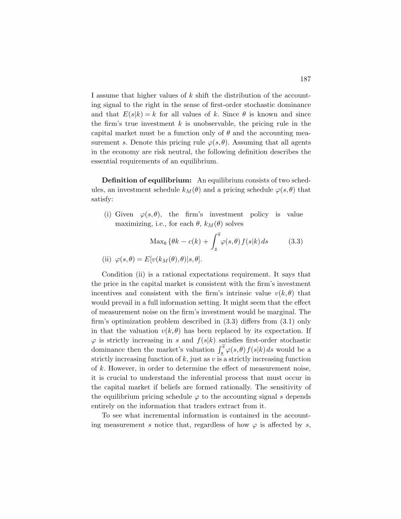
I assume that higher values of k shift the distribution of the account-ing signal to the right in the sense of first-order stochastic dominanceand that E(s|k) = k for all values of k. Since θ is known and sincethe firm’s true investment k is unobservable, the pricing rule in thecapital market must be a function only of θ and the accounting mea-surement s. Denote this pricing rule ϕ(s,θ). Assuming that all agentsin the economy are risk neutral, the following definition describes theessential requirements of an equilibrium.
Definition of equilibrium: An equilibrium consists of two sched-ules, an investment schedule kM (θ) and a pricing schedule ϕ(s,θ) thatsatisfy:
(i) Given ϕ(s,θ), the firm’s investment policy is valuemaximizing, i.e., for each θ, kM (θ) solves
Maxk θk − c(k) +∫ s
sϕ(s,θ)f(s|k)ds (3.3)
(ii) ϕ(s,θ) = E[v(kM (θ),θ)|s,θ].Condition (ii) is a rational expectations requirement. It says that
the price in the capital market is consistent with the firm’s investmentincentives and consistent with the firm’s intrinsic value v(k,θ) thatwould prevail in a full information setting. It might seem that the effectof measurement noise on the firm’s investment would be marginal. Thefirm’s optimization problem described in (3.3) differs from (3.1) onlyin that the valuation v(k,θ) has been replaced by its expectation. Ifϕ is strictly increasing in s and f(s|k) satisfies first-order stochasticdominance then the market’s valuation
∫ ss ϕ(s,θ)f(s|k)ds would be a
strictly increasing function of k, just as v is a strictly increasing functionof k. However, in order to determine the effect of measurement noise,it is crucial to understand the inferential process that must occur inthe capital market if beliefs are formed rationally. The sensitivity ofthe equilibrium pricing schedule ϕ to the accounting signal s dependsentirely on the information that traders extract from it.
To see what incremental information is contained in the account-ing measurement s notice that, regardless of how ϕ is affected by s,
188 Real Effects of Imprecision in Accounting Measurements
(3.3) indicates that the firm’s equilibrium investment is a functiononly of θ. Since θ is a priori known to traders in the capital mar-ket they can perfectly anticipate the firm’s equilibrium investment.Given such perfect anticipation, the noisy accounting measurement s
conveys no incremental information and the conditioning effect of s
in (ii) is vacuous. Thus, the equilibrium pricing rule ϕ that prevailsin the capital market cannot be a function of s and is describedby some schedule ϕ(θ) that incorporates the market’s anticipationof the firm’s investment. Given the equilibrium valuation sched-ule ϕ(θ) the firm’s investment choice problem becomes Maxk θk −c(k) + ϕ(θ), which yields the first-order condition c′(k) = θ. I haveestablished,
Proposition 3.1. When the firm’s investment is measured impreciselyand its profitability parameter θ is common knowledge, the firm’s equi-librium investment schedule is described by c′(kM (θ)) = θ and the equi-librium price schedule in the capital market is v(kM (θ),θ), ∀s.
Proposition 3.1 says that the real effect of noise in the account-ing measurement of investment is that it induces the firm to investmyopically so as to maximize only the short-term return to invest-ment and completely ignore the effect of its investment on long-termreturns. If the marginal effect of investment on long-term returns islarge the magnitude of underinvestment would be substantial. Themarket is not fooled by the cutting back of investment from firstbest levels — so the equilibrium I have characterized is fully consis-tent with the efficient markets hypothesis. The market correctly antic-ipates myopic investment and prices the firm accordingly. In turn, thefirm optimally responds to market pricing and invests myopically. Thefirm and its shareholders are trapped in a very bad, but fully ratio-nal, equilibrium where substantial value is destroyed. Any noise in theaccounting measurement of investment completely destroys its infor-mation content, even though there is a well defined statistical rela-tionship between the accounting signal and the level of the firm’sinvestment. The intuition for why the accounting report is ignored isthat, given their knowledge of θ, traders in the capital market can

189
step into the shoes of management and solve the investment problemof the firm. Thus, the capital market rationally believes it perfectlyknows the firm’s investment even though it cannot actually see thatinvestment. When the market observes an accounting report of invest-ment that does not coincide with its perfect anticipation it attributesthe difference to measurement noise and ignores the accountingreport.
To get a sense of magnitudes, suppose the real investment cost isquadratic and the perfect information pricing rule is linear in invest-ment, i.e., c(k) = 1
2ck2 and v(k,θ) = γkθ, γ > 0. Then first best invest-ment is kFB(θ) =
(1+γc
)θ, while myopic investment is kM (θ) =
(1c
)θ.
Thus if γ = 10, corresponding to a price earnings multiple of 10,myopic investment would be one-eleventh of first best investmentand the value of the firm would be one-eleventh of its first bestvalue.
The results obtained here are starkly different from the insights pro-vided by models of pure trade, such as CAPM, that have been used intraditional studies of disclosure. In these models the distribution of thefirm’s liquidating dividend is exogenous and independent of measure-ment noise, which is equivalent to holding the firm’s investment fixed.The effect of measurement noise is to simply decrease the precisionwith which the firm’s liquidating dividend is estimated. When tradersin the capital market are risk averse, this decreased precision of esti-mates is translated into higher risk premiums and therefore lower equi-librium market valuations. But the higher risk premium which arisesdue to measurement noise is at most a small second-order effect onmarket valuations, while the real effect of reduced investment on mar-ket valuations is an order of magnitude larger first-order effect. Thesimple model developed here illustrates my earlier claim that the dis-closure insights obtained from models of pure trade could be seriouslyin error.
The myopia result described in Proposition 3.1 is logically consis-tent but unrealistic. Although imprecision in accounting measurementof investment is an undeniable empirical fact, it is unlikely that suchnoisy measurements are completely ignored in the capital market andit is unlikely that firm’s invest in such an extreme myopic fashion. This
190 Real Effects of Imprecision in Accounting Measurements
suggests that the environment modeled here is not rich enough to yieldempirically sustainable results regarding the real effects of account-ing imprecision. The most unrealistic feature of this model is that itpermits outsiders to step into the shoes of management and perfectlyanticipate the firm’s investment. A likely reason why outsiders are real-istically unable to perfectly anticipate managerial actions is that theydo not have full access to the information that managers collect and usein making their decisions. The market has been assumed to know toomuch! Shareholders delegate decision making to corporate managersprecisely because they do not have the time, expertise and incentivesto continually keep track of new information and emerging opportu-nities. This suggests that a much more plausible setting for the studyof accounting imprecision is one where the profitability parameter θ
is privately known only to the firm’s managers and this informationcannot be directly communicated to the capital market. Notice that insuch settings an investment policy k(θ) in conjunction with an assessedprior distribution on θ would yield a prior distribution on the firm’sinvestment. Imprecise measurement of the firm’s investment would thenacquire information content and would be used in a Bayesian fashionto update the capital market’s assessment of how much investment hasoccurred.
Before we study the effects of accounting imprecision in this setting,let us determine the equilibrium that would be achieved if accountingmeasurements of investment were infinitely precise. Now, by assump-tion, when the firm invests k the market perfectly observes this fact,but the market also knows that the manager chooses investment inthe light of information about its profitability θ that the market doesnot know. Thus, in evaluating the cash flow consequences of an invest-ment of k, traders in the capital market must necessarily make infer-ences about the value of θ that must have been observed by managerswhen they chose k units of investment. Thus, in addition to affectingthe distribution of future cash flows, the firm’s investment acquires aninformational value. This raises the possibility of a Spence-type (1974)signalling equilibrium, where perfect measurement of the firm’s invest-ment results in perfect inferences of the firm’s profitability parameter θ.

191
Indeed such an equilibrium exists1 and is defined and characterizedbelow.
Definition of equilibrium: A fully revealing signalling equilib-rium is a triple of schedules, an investment schedule k(θ), a pricingschedule ϕ(k), and an inference schedule I(k) that satisfy:
(i) k(θ) = arg maxk θk − c(k) + ϕ(k)(ii) ϕ(k) = v(k,I(k)), and(iii) I(k(θ)) = θ, ∀θ.
Notice that the equilibrium pricing schedule in the capital marketmust be a function of k alone because θ is unknown to the capital mar-ket. However, embedded in this pricing schedule are the capital mar-ket’s inferences about the underlying value of θ that the firm’s managermust have observed when k was chosen. Condition (ii) of equilibriumsays that if the market makes the perfect inference that the value ofθ is I(k), then the equilibrium price in the capital market must cor-respond to the equilibrium price in a fully informed market given theobserved k and the inferred value of θ, i.e., ϕ(k) = v(k,I(k)). Condition(iii) of equilibrium is the standard rational expectations requirementof any fully revealing signalling equilibrium — the inferred value of θ
from any observed k is indeed the true value of θ that produced thatk. Condition (i) of the equilibrium says that the firm takes the pric-ing schedule in the capital market as given and chooses investment tomaximize its cum-dividend value.
There appears to be a misconception in the accounting literaturethat in a signalling equilibrium the informed agent seeks to consciouslysignal his/her information to the uninformed and looks for ways todo so. Such a deliberate attempt to communicate would be more inthe spirit of cheap talk games, as in Crawford and Sobel (1982). Here,the firm is not choosing to consciously signal its information. The firm
1 Technically, a fully revealing signalling equilibrium requires the satisfaction of a singlecrossing property (equivalently, the Spencian cost condition) in the firm’s payoff struc-ture. The existence of short-term returns to investment, as modeled, and their privateconsumption guarantees that this condition is met.

192 Real Effects of Imprecision in Accounting Measurements
simply responds optimally to the way in which its investment is pricedin the capital market and does not even need to be aware of the factthat the capital market is making inferences from the investment itchooses. Moreover, the capital market must form beliefs about theprofitability of investment in order to rationally price the firm, andthe rational expectations (or efficient markets) hypothesis requires thatthese beliefs are not arbitrary, but are consistent in some sense withthe investment policy actually chosen by the firm. The structure ofpayoffs here is such that the interrelationship between rationality ofbeliefs and the optimality of investment is fulfilled at a fully revealingequilibrium.2
Given the fully revealing nature of the equilibrium, an empiricalstudy of a new accounting standard that somehow required the firmto verifiably disclose its information about θ to the capital marketbefore choosing its investment, would reveal that the new disclosurehas no incremental information content. It would be deceptive toconclude that such a disclosure requirement serves no purpose. Itwill become obvious momentarily that such a disclosure policy, if itcould be implemented, would significantly change the firm’s invest-ment policy and its capital market price and thus have substantialreal effects, without changing the information in the capital market.How information reaches the capital market, through an inferentialprocess or through direct disclosure, is of fundamental importance.It is not enough to simply assess and compare the information inthe capital market in a pre-disclosure regime to a post-disclosureregime.
Proposition 3.2. When the profitability of investment θ is known tothe firm’s manager but unknown to the capital market, perfect mea-surement of investment induces the firm to over-invest relative to firstbest levels. The firm’s equilibrium investment is characterized by the
2 In settings such as we are studying, there is usually also a degenerate equilibrium where thecapital market simply uses the prior mean of θ to evaluate the firm’s investment andthe firm responds by choosing the same level of investment for every value of θ. How-ever, the off-equilibrium beliefs required to sustain such equilibria are implausible, giventhat there is also a fully revealing equilibrium.

193
first-order differential equation,
k′(θ)[c′(k(θ)) − θ − vk(k(θ),θ)] = vθ(k(θ),θ) (3.4)
k′(θ) > 0, k(θ) = kFB(θ), (3.5)
where the support of the prior distribution of θ is the interval [θ ,θ]
Proof. It is convenient to use the mechanism design methodologyto characterize the equilibrium.3 Since any equilibrium allocation(fully revealing or not) must be incentive compatible, the equilib-rium investment schedule k(θ) must be such that if θ′ and θ aretwo values of θ ∈ [θ ,θ] then the manager who observes θ′ must pre-fer to invest k(θ′) to an investment of k(θ) and when the managerobserves θ he/she would rather invest k(θ) than k(θ′). If, in addi-tion, the equilibrium is fully revealing then an investment of k(θ′)must lead to the inference that θ = θ′, and an investment of k(θ)must lead to the inference that θ = θ. Thus any fully revealing equilib-rium investment schedule must satisfy the incentive compatibility (IC)requirements:
θk(θ) − c(k(θ)) + v(k(θ),θ) ≥ θk(θ) − c(k(θ)) + v(k(θ), θ), ∀θ, θ.
(3.6)Denote the left-hand side of (3.6) by Ω(θ), so that the incentive com-patibility constraints can be equivalently expressed as
Ω(θ) ≥ Ω(θ) − k(θ)[θ − θ], ∀θ, θ. (3.7)
Reversing the roles of θ and θ yields an equivalent reverse IC constraint,
Ω(θ) ≥ Ω(θ) − k(θ)[θ − θ], ∀θ, θ. (3.8)
Equations (3.7) and (3.8) together imply that the equilibrium schedulesΩ(θ),k(θ) must satisfy,
k(θ)[θ − θ] ≤ Ω(θ) − Ω(θ) ≤ k(θ)[θ − θ], ∀θ, θ. (3.9)
3 The equivalence of the Spence-Riley methodology and the mechanism design methodologyfor constructing a signalling equilibrium is developed in Kanodia and Lee (1998).

194 Real Effects of Imprecision in Accounting Measurements
I now claim that an investment schedule k(θ) is incentive compati-ble and fully revealing if and only if (i) Ω′(θ) = k(θ) and (ii) k(θ)is increasing. The claim that k(θ) is necessarily increasing followsdirectly from the left-hand and right-hand side inequalities in (3.9).In turn, this implies that k(θ) must be continuous almost everywhere.Dividing (3.9) by (θ − θ), taking the limit as θ → θ and using thecontinuity of k(θ) yields the result that Ω(θ) is differentiable almosteverywhere and Ω′(θ) = k(θ). This establishes the necessity part ofclaims (i) and (ii).
Now to establish sufficiency it must be shown that the satisfactionof (i) and (ii) imply that incentive compatibility is satisfied. From (i)it follows that ∫ θ
θΩ′(t)dt =
∫ θ
θk(t)dt. (3.10)
Consider θ > θ. Then (3.10) implies,
Ω(θ) = Ω(θ) +∫ θ
θk(t)dt. (3.11)
Now if k(θ) is increasing, as claimed in (ii), (3.11) implies Ω(θ) ≤Ω(θ) + k(θ)[θ − θ]. Rearranging terms yields the incentive compatibil-ity condition Ω(θ) ≥ Ω(θ) − k(θ)[θ − θ], ∀θ > θ. Now, consider θ < θ.Then from (3.10) it follows that Ω(θ) = Ω(θ) +
∫ θθ k(t)dt ≥ Ω(θ) +
k(θ)[θ − θ], where the last inequality follows from claim (ii).Since claims (i) and (ii) are necessary and sufficient for incentive
compatibility, any fully revealing equilibrium investment schedule mustsatisfy those claims. From (i) it follows that,
Ω(θ) = Ω(θ) +∫ θ
θk(t)dt. (3.12)
Replacing the left-hand side of (3.12) by the definition of Ω(θ), it followsthat k(θ) must satisfy,
θk(θ) − c(k(θ)) + v(k(θ),θ) = Ω(θ) +∫ θ
θk(t)dt. (3.13)

195
Differentiating (3.13) with respect to θ gives
k(θ) + θk′(θ) − c′(k(θ))k′(θ) + vk(k(θ),θ)k′(θ) + vθ(k(θ),θ) = k(θ).
Rearranging and collecting common terms yields (3.4).The result that the firm over-invests at every θ > θ follows directly
from (3.4). Since k′(θ) > 0 in any fully revealing signalling equilib-rium and since vθ > 0 it is necessary that c′(k(θ)) − θ − vk(k(θ),θ) > 0whereas first best investment satisfies c′(k(θ)) − θ − vk(k(θ),θ) = 0.This completes the proof.
Again, to get a sense of magnitudes let us return to the exampleI considered earlier. Assume c(k) = 1
2ck2 and v(k,θ) = γkθ, γ > 0. Forthis example, and with the additional assumption that θ = 0, the solu-tion to the differential equation (3.4) is
kPS(θ) =(
1 + 2γ
c
)θ.
Thus, if γ = 10, the investment that is induced by perfect measure-ment is almost twice as much as in the first best setting. Onceagain the firm is trapped in a bad equilibrium. I have shown thatwhen the profitability parameter θ is publicly known, imprecise mea-surements of investment induce the firm to under-invest, and whenθ is privately known only to the firm’s manager perfect measure-ments of the firm’s investment induce the firm to over-invest. Theseresults suggest that perhaps some ignorance of θ in the capital marketand some imprecision in the measurement of investment may actu-ally improve the equilibrium and sustain investment levels that arecloser to first best. Ignorance of the project’s profitability preventsperfect anticipation of the firm’s investment and allows imprecise mea-surements to acquire information content, thus alleviating the under-investment problem. Imprecision in measuring the firm’s investmentcounteracts the firm’s incentive to over-invest when the project’s prof-itability is unknown to the capital market and the market is forcedto make inferences about it. The results derived below confirm thisintuition.
Assume, now, that the manager privately observes the profitabilityparameter θ before choosing the firm’s investment and that investment
196 Real Effects of Imprecision in Accounting Measurements
is measured imprecisely and reported to the capital market. The mar-ket views θ as a drawing from a probability distribution with densityh(θ) and support Θ, and observes only the imprecise measurement s
of the firm’s investment where the measurement noise is described bythe probability density f(s|k) described earlier. Now the price in thecapital market will be a function only of the accounting report s, sayϕ(s), since that is only variable observed by capital market traders.Embedded in this price schedule is the market’s inferences about boththe firm’s investment and the profitability parameter θ, conditional onthe observed value of s.
Let us first examine the nature of inferences that the capital marketwill need to make. Given that the accounting measurement s is noisy, itis clear that the capital market is unable to make perfect inferences ofeither k or θ. The capital market will need to assess posterior distribu-tions of k and θ conditional on s. In order to do this, the market needsto conjecture an investment policy k(θ) that describes beliefs about howthe firm would choose an investment level contingent on each value of θ
that the manager could observe. Given such a conjectured investmentpolicy, an assessed posterior distribution on θ would statistically implya posterior distribution on k, so no further assessments are needed. Letg(θ|s) be the assessed posterior density of θ. Rational assessments mustsatisfy Bayes rule,
g(θ|s) =f(s|k(θ))h(θ)∫
Θf(s|k(t))h(t)dt
. (3.14)
Notice that the investment policy conjectured by the market isembedded in this posterior calculation and the probability densityfunction of s at θ is described by the measurement noise f(s|k)and the belief that at θ the firm will invest k(θ). Expectationsare rational (equivalently, markets are efficient) if the investmentpolicy conjectured by the market is the same as the investment pol-icy induced by the market’s Bayesian assessments that are incorpo-rated into market valuations. This leads to the following definition ofequilibrium.
197
Definition of equilibrium: An equilibrium is a triple of func-tions, an investment schedule k(θ), Bayesian posteriors g(θ|s), and avaluation schedule ϕ(s) that satisfy:
(i) Given ϕ(s), the investment policy of the firm is value maxi-mizing, i.e., k(θ) solves:
Maxk
[θk − c(k) +
∫ s
sϕ(s)f(s|k)ds
](ii) g(θ|s) satisfies (3.14), and(iii) ϕ(s) =
∫Θ v(k(θ),θ)g(θ|s)dθ.
This definition describes a noisy signalling equilibrium. The firm’schoice of investment has information content since it affects theaccounting measurement of s, but this information content is diluted bythe measurement noise in f(s|k). Because of this noise, the inferencesmade by the market are probabilistic in nature and these probabilisticinferences are reflected in the equilibrium valuation schedule ϕ(s). Asdescribed in (iii), the valuation schedule in the market reflects a poolingof types but this is not the usual kind of pooling. The weights g(θ|s)are equilibrium weights that emerge endogenously. They depend notonly on the prior density h(θ), but also on the measurement noise inf(s|k) and the endogenous investment policy of the firm k(θ). Since theinvestment policy affects these weights, it affects the firm’s valuation inthe capital market, thus stimulating the firm to invest more than themyopic amount (see KSS, Corollary to Proposition 3).
The first-order condition to the firm’s optimization problem is
θ − c′(k) +∫ s
sϕ(s)f k(s|k)ds = 0.
Inserting the equilibrium conditions (ii) and (iii) into this first-ordercondition yields:∫ s
s
[∫Θv(k(t), t)
f(s|k(t))h(t)∫Θf(s|k(τ))h(τ)dτ
dt
]fk(s|k(θ))ds = c′(k(θ)) − θ
(3.15)

198 Real Effects of Imprecision in Accounting Measurements
Equation (3.15) is an integral equation with a single unknown, theinvestment schedule k(θ). KSS (see their Proposition 3) establishthat any investment schedule that is increasing in θ and satisfies(3.15) is an equilibrium investment schedule. In order to shed lighton the economic consequences of accounting imprecision it is nec-essary to examine how the equilibrium investment schedule wouldchange with the amount of noise in f(s|k). Unfortunately, the inte-gral equation (3.15) is too complex to accomplish this task withoutadditional specificity to the model. Therefore, I make the followingadditional assumptions, which are slightly stronger than those madein KSS.
(A1) s = k + ε, where ε is Normally distributed noise withE(ε) = 0, var(ε) = σ2
ε .(A2) The prior distribution of θ is Normal with E(θ) = 0, var(θ) =
σ2θ .
(A3) v(k,θ) = γkθ, γ > 0.(A4) c(k) = 1
2ck2.
The assumption of Normally distributed random errors allows a pre-cise specification of the amount of noise (σ2
ε ) that is present in account-ing measurements of investment. Assumption (A2) together with (A1)facilitates Bayesian updating, and Assumptions (A3) and (A4) permitlinear investment schedules to be sustained as equilibria. With theseassumptions, the integral equation (3.15) can be explicitly solved, asshown below.4
To construct the equilibrium described by (3.15), let us begin withthe conjecture (to be confirmed later) that the equilibrium investmentschedule is linear in θ, i.e., k(θ) = a + bθ, b > 0. Given such an invest-ment schedule the noisy measurement s can be represented as:
s = k(θ) + ε = a + bθ + ε.
4 The literature on noisy signalling is extremely sparse. There is no standard methodologyfor constructing and analyzing such equilibria. The approach taken by KSS is new in theliterature.

199
Thus the joint distribution of (θ, s) is Normal, and the conditionaldensity g(θ|s) is also Normal with parameters:
E(θ|s) = β
(s − a
b
), var(θ|s) = (1 − β)σ2
θ , (3.16)
where β = b2σ2θ
b2σ2θ +σ2
ε. Additionally,
ϕ(s) = E θ [γk(θ)θ|s] = aγE(θ|s) + bγE(θ2|s).Since E(θ2|s) = var(θ|s) + E2(θ|s), it follows from (3.16) that
ϕ(s) = aγβ
(s − a
b
)+ bγ(1 − β)σ2
θ + bγβ2(
s − a
b
)2
, (3.17)
which has the quadratic form:
ϕ(s) = α0 + α1s + α2s2. (3.18)
The parameters α0,α1,α2 can be calculated by matching the coefficientsin (3.18) with the corresponding coefficients in (3.17). Also, if f(s|k) isa Normal density with mean k and variance σ2
ε , f k(s|k) = f(s|k)[ s−kσ2
ε].
Using these facts, the left-hand side of the integral equation (3.15)can be expressed as∫
ϕ(s)f k(s|k)ds =1σ2
ε
[α0E(s − k|k) + α1[E(s2|k) − kE(s|k)]
+α2[E(s3|k) − kE(s2|k)]]
=1σ2
ε
[α1(σ2
ε + k2 − k2)
+α2(k3 + 3kσ2ε − k3 − kσ2
ε )]
= α1 + 2α2k.
The above characterization together with (3.15) implies that equilib-rium investment at each θ is characterized by the equality α1 + 2α2k =ck − θ, or equivalently,
k(θ) =α1
c − 2α2+(
1c − 2α2
)θ, (3.19)
which confirms the linear conjecture made earlier.
200 Real Effects of Imprecision in Accounting Measurements
In order to obtain insights into how accounting imprecision affectssustainable investment levels, it is necessary to relate the coefficientsa and b of the linear investment schedule k(θ) = a + bθ to the impre-cision parameter σ2
ε . It is convenient to do this in a backdoor way bycharacterizing the values of β,a, and σ2
ε in terms of b. From (3.19),b =
( 1c−2α2
)and a = α1b. By matching coefficients in (3.17) and (3.18),
we determine that α2 = γβ2
b and α1 = aγβb − 2aγβ2
b . Inserting the valueof α2 into the equation for b yields bc − 2γβ2 = 1, or equivalently,
β =
√bc − 1
2γ. (3.20)
Inserting the value of α1 into the equation for a gives,
a [1 − γβ + 2γβ2] = 0. (3.21)
Inserting β = b2σ2θ
b2σ2θ +σ2
εin (3.20) and solving for σ2
ε gives,
σ2ε = b2σ2
θ
[√2γ
bc − 1− 1
]. (3.22)
Equilibrium investment schedules are constructed by choosing a“sustainable” value of b, then solving for β from (3.20), then solv-ing for a from (3.21) and lastly solving for σ2
ε from (3.22). Sustainablevalues of b are those that result in values of σ2
ε that lie in the interval(0,∞). I first characterize the values of b that are sustainable by corre-
sponding values of σ2ε . From (3.22), σ2
ε ≥ 0 if and only if√
2γbc−1 − 1 ≥ 0
which, in turn, requires that b ≤ 1+2γc . Also since it is necessary that
bc − 1 ≥ 0, sustainable values of b must satisfy b ≥ 1c . Any value of b
intermediate to these two extremes is also sustainable since (3.22) willyield a positive and finite value of σ2
ε for all such intermediate val-ues. However, the equilibrium investment schedule is not necessarilyunique for exogenously given values of σ2
ε , since the solution for b isnot always unique. The remaining parameter a of the linear equilib-rium investment schedule must satisfy (3.21), from which it followsthat if the quantity [1 − γβ + 2γβ2] = 0 then the intercept a must nec-essarily be zero. Since [1 − γβ + 2γβ2] is a quadratic expression it can

201
attain a value of zero for at most two values of β, in which case thereare multiple equilibria. However, any plausible equilibrium investmentschedule must have a = 0, since otherwise the firm would be investingeven though the profitability of investment θ is zero. We have thusestablished:
Proposition 3.3. Given assumptions (A1) through (A4), when theprofitability of investment θ is known to the firm’s manager butunknown to the capital market, and the firm’s investment is measuredimprecisely, the equilibrium investment schedule has the linear formk(θ) = bθ. The value of the parameter b depends on the amount of noise(σ2
ε ) in accounting measurements. Any b in the interval 1c ≤ b ≤ 1+2γ
c
is sustainable by some corresponding value of σ2ε .
Notice that b = 1c corresponds to managerial myopia and b = 1+2γ
c
corresponds to perfect signalling. These two extremes are realized whenσ2
ε → ∞ and when σ2ε → 0, respectively. Since the first best investment
schedule corresponds to b = 1+γc , Proposition 3.3 indicates that there
is some level of accounting imprecision that would stimulate the firmto invest at first best levels. This is, indeed, the optimal level of impre-cision in accounting measurements and that optimal level is not zero.Substituting b = 1+γ
c in (3.22) and solving for σ2ε yields the optimal
level of imprecision characterized in the proposition below.
Proposition 3.4. Given assumptions (A1) through (A4), when theprofitability of investment θ is known to the firm’s manager butunknown to the capital market, there is an optimal non-zero degreeof imprecision (σ2
ε ) in accounting measurements of investment, charac-terized by:
σ2ε = σ2
θ
(1 + γ
c
)2 [√2 − 1
]. (3.23)
The greater the degree of information asymmetry (σ2θ) between the
manager and the market regarding the profitability of the firm’s invest-ment and the higher the price-earnings multiple (γ) the greater is theoptimal degree of imprecision.

202 Real Effects of Imprecision in Accounting Measurements
What is important in the above results is not the precise algebraiccalculations that are essential to any scientific investigation of account-ing issues, but the qualitative insights that are obtained from them. Itwould clearly be difficult for a regulatory body like the FASB to man-date a certain level of imprecision in accounting measurements, or evento calculate the optimal level of imprecision. However, the guiding prin-ciple, suggested by traditional studies of disclosure, that imprecision inaccounting measurements is always harmful and should be eliminatedto the extent possible, does not hold up in many plausible settingswhen the real effects of such imprecision are taken into account. Insuch settings, some degree of accounting imprecision is actually valueenhancing. More often than not, while accounting reports can com-municate managerial actions the informational basis for those actionsremains hidden from the market and cannot immediately be reflected inaccounting reports. The market must necessarily make inferences aboutthe hidden information in order to assess the cash flow consequencesof managerial actions and price the firm accordingly. Proposition 3.4yields the qualitative insight that the greater the information asym-metry regarding the information underlying managerial actions, thegreater should be our tolerance for imprecision in measuring and report-ing those actions.
4Real Effects of Measuring Intangibles
Examples of intangible investments are expenditures on research anddevelopment, information technology, human capital, brand equity, pro-cess improvements, etc. The last decade witnessed an explosive growthin such intangible investments reflecting their increased importance inthe new economy. It is now felt that many firms derive their compet-itive advantage mostly from investments in intangibles. The currentaccounting treatment of intangible assets requires a firm’s R&D expen-ditures to be listed as a separate line item in the income statement butdoes not allow its capitalization. All other expenditures on intangiblesare left comingled with operating expenses with no attempt to measureand report them separately.
In the academic literature there is a great deal of dissatisfactionwith the current accounting treatment of intangibles. Lev and Zarowin(1999), Healy et al. (2002), and many others using the “value relevance”approach to disclosure, have shown that empirically the capital marketappears to price the firm as if expenditures on intangibles are assets.Hence, they argue, accountants’ refusal to measure and capitalize suchexpenditures has caused a serious decline in the relevance and useful-ness of financial statements. On the other hand, the FASB has argued
203

204 Real Effects of Measuring Intangibles
that attempts to capitalize intangibles would seriously impair the reli-ability of accounting statements because intangible assets cannot bemeasured with reasonable precision, and attempts to measure themwould open the floodgates to earnings management by unscrupulousmanagers. The debate remains unsettled.
Kanodia, Sapra and Venugopalan (KSV) (2004) investigated thereal effects of measuring intangibles. They assume that intangiblesare value relevant, in the sense that such investments stochasticallyincrease future cash flows. They also assume that attempts to mea-sure intangibles would introduce several kinds of noise in accountingdata. Thus, their analysis gives credence to both sides of the debate.KSV argue that the value relevance approach is inconclusive becausestatistical associations between accounting data and stock prices donot by themselves identify economic consequences. If the statisticalassociations change depending on the accounting treatment of intan-gibles but nothing else in the economy changes such as firms’ invest-ments, cash flows and stock prices, then these statistical associations areof purely academic interest and lack any policy significance. Insightsinto the controversy are better developed by exploring the real eco-nomic consequences of measurement versus non-measurement takinginto account both the value relevance of intangibles and the noise intro-duced by their measurement. My discussion here is based on the KSVarticle.
Consider a setting where a firm is choosing how much to invest intangible and intangible assets. The marginal return to each kind ofasset depends on how much the firm has invested in the other. Thisassumption is consistent with the intuition that tangible and intangi-ble assets compliment each other rather than substitute for each other.More specifically, KSV assume that tangible and intangible assets com-bine in a Cobb Douglas like fashion to form the capital stock of thefirm and future cash flows are stochastically related to the firm’s capitalstock. Let
q = the firm’s capital stock,K = the firm’s investment in tangible assets, andN + γ = the firm’s expenditure on intangible assets.

205
The random variable γ, distributed Normally with zero mean andvariance σ2
γ , captures an assumption that some random component γ
of expenditures on intangibles is wasteful and unproductive1 — theproductive component is N . I assume,
q = KαNβ, α > 0, β > 0, α + β < 1. (4.1)
The assumption α + β < 1 is inconsistent with the Cobb Douglas tech-nology, but guarantees the strict concavity of q in K and N . The firmchooses its investments at date 0. At dates 1 and 2, these investmentsyield stochastic cash flows x1 and x2, respectively. Assume that (x1, x2)is joint Normally distributed with,
E(x1) = E(x2) = qµ,
Cov(x1, x2) = ρ > 0,
Var(x1) = σ2x
ρ ≤ σ2x
In the above specification µ > 0 is a commonly known profitabilityparameter. The larger the value of µ the more value relevant is thefirm’s investments. To keep the analysis simple, I have assumed thatthe firm’s capital stock increases expected cash flows but does notaffect the covariance or variance of cash flows. The assumption thatthe covariance of cash flows is positive is essential to the analysis, andthe assumption ρ ≤ σ2
x implying that Cov(x1, x2) ≤ Cov(x1, x1) canbe replaced by a weaker but more messy assumption, but it seemsreasonable.
The firm maximizes its expected date 1 price, taking the market’svaluation rule as given, and this date 1 price P is specified as,
P = Net cash assets at date 1 + E(x2|information).
This specification assumes risk neutral pricing in the market and anyknown cash balance in the firm is valued dollar for dollar. The net cashbalance at date 1 is,
z = x1 − K − N − γ. (4.2)
1 The realism of this feature of intangible investments is apparent to any one who hasengaged in research or human capital development. It is essential to the analysis, as willbecome apparent later.

206 Real Effects of Measuring Intangibles
Since cash balances are measured perfectly and reported in virtuallyevery accounting regime, I assume that the date 1 cash balance z,but not necessarily its components, is publicly known in each of theinformational regimes to be discussed.
At date 1, the primitives describing the firm’s operations are:
K = the firm’s tangible assets,N = the firm’s productive intangible assets,N + γ = the total expenditure on intangibles,x1 = the true operating income of the firm in the first period.
None of these primitive variables are observed directly by the capitalmarket. Instead, the market observes accounting reports consisting of
IK = measured tangible assets,IN = measured intangible assets,z = the firm’s cash balance at date 1, andy = reported income.
These measurements will differ from one informational regime toanother in the manner specified below. I examine three informationalregimes: a Utopian full information regime where accounting is per-fect, an expensing regime where no attempt is made to measure thefirm’s intangible assets, and an intangibles measurement regime wherethe firm’s intangibles are measured and reported with noise. I usethe superscripts u,e, and m to denote measurements in the Utopianregime, the expensing regime and the intangibles measurement regime,respectively.
In the Utopian regime, tangible investments are measured perfectly,accountants can perfectly observe the total expenditure on intangiblesand can perfectly discriminate between unproductive and productiveexpenditures. Hence, the accounting reports produced are:
IuK = K,
IuN = N,
yu = x1 − γ, where γ is reported separately from the true operatingincome of x1, and
zu = x1 − K − N − γ.

207
Of course, the Utopian regime never exists. It is included here toprovide a benchmark against which more realistic accounting regimescan be compared.
In the expensing regime, I continue to assume that tangible assetscan be measured perfectly, but since no attempt is made to measureand analyze the expenditures on intangibles, such expenditures remaincomingled with the operating expenditures that when deducted fromrevenues determines the firm’s operating income. The expression for netcash balance z is unchanged. Thus the accounting reports produced inthe expensing regime are
IeK = K,
ye = x1 − N − γ, and
ze = x1 − K − N − γ.
The measurement of intangibles is limited by several factors, andeach of them introduces noise in accounting reports. First, there isno reason to believe that accountants have the ability to discriminatebetween productive and unproductive expenditures on intangibles. So Iassume that both are treated the same way. Second, consistent with theconcerns of the FASB, I assume that the boundary between operatingexpenditures and expenditures on intangible assets is fuzzy so attemptsto measure intangibles will result in some operating expenditures beingclassified as assets and some intangible assets being classified as oper-ating expenditures. Third, an accounting regime that seeks to measureintangibles is much more permissive than an expensing regime. In anexpensing regime any doubt about the nature of an observed cash out-flow results in immediate expensing of that cash outflow. In a morepermissive regime such is not the case, causing contamination in themeasurement of tangible assets also. I model this as random misclas-sification between tangible and intangible assets. Thus, the accountingreports produced in the intangibles measurement regime are
ImK = K + η
ImN = N + γ − η + ω
zm = x1 − K − N − γ

208 Real Effects of Measuring Intangibles
ym = z + IK + IN
= x1 − K − N − γ + (K + η) + (N + γ − η + ω)
= x1 + ω.
I have introduced two new random variables, η and ω. The randomvariable η represents classification errors between tangible and intan-gible assets. Therefore, its effect is offsetting in the measurements Im
K
and ImN . The random variable ω represents misclassifications between
operating expenditures and expenditures on intangible assets. I assumethat η and ω are Normally distributed with zero means and finite vari-ances σ2
η and σ2ω, respectively. They are independent of each other and
independent of γ. Consistent with the way in which accountants calcu-late a firm’s earnings, reported income is always specified as observednet cash flow adjusted by accruals. The only accruals here are measuredtangible and intangible assets.
There are important informational differences between the theexpensing regime and the intangibles measurement regime. In theexpensing regime the firm’s net cash flow can also be expressed asze = ye − K. Since K is perfectly reported, the firm’s net cash flowcontains no information incremental to that contained in the reportedincome number. As in our previous discussion of imprecision in account-ing measurements of investment, it will turn out that the stock marketwill form rational beliefs of the firm’s investment in intangibles so that,in equilibrium, both reported income ye and net cash flow ze will com-municate the noisy estimate x1 − γ of the firm’s true operating income.In the intangibles measurement regime the firm’s net cash flow zm com-municates x1 − γ, while reported income ym communicates x1 + ω.Since γ and ω are independent, the firm’s net cash flow contains infor-mation incremental to that contained in reported income. Because ofthis feature, the intangibles measurement regime provides strictly moreinformation about the firm’s true operating income x1than the expens-ing regime. However, the measurement of intangibles contaminates themeasurement of tangible investments, so there is less information aboutthe latter. Thus the two regimes are not Blackwell comparable.
Let us now examine the firm’s investment choices in the three infor-mational regimes. In the Utopian regime, at date 1 the capital market
209
perfectly knows the values of z,x1,K,N , so that the date 1 price ofthe firm is
P (z,x1,K,N) = z + E(x2|x1,K,N).
At date 0, the firm chooses K and N to maximize the expected date 1price, i.e.,
MaxK,N E0(x1 − K − N − γ) + E0(E(x2|x1,K,N)),
where E0 denotes an expectation taken at date 0. SinceE0(E(x2|x1,K,N)) = E0(x2|K,N)) = E0(x1|K,N)) = µKαNβ, thefirm’s optimization collapses to
MaxK,N 2µKαNβ − K − N.
The first-order conditions describing the firm’s optimal investments are
2µαKα−1Nβ = 1, (4.3)
2µβKαNβ−1 = 1 (4.4)
and the firm invests in tangibles and intangibles in the efficient ratio,
K
N=
α
β. (4.5)
This implies that the technological parameters α and β also indicatethe relative importance of each kind of investment. The larger is thevalue of β relative to α, the greater will be the proportion of intangiblesin the firm’s capital stock.
Let us now turn our attention to the expensing regime. I earlierindicated that the information contained in the accounting reports canbe summarized by the tuple K,ye. Since the net cash assets of thefirm at date 1 is ze = ye − K, the date 1 price schedule in the capitalmarket is
P (K,ye) = ye − K + E(x2|K,ye).
In order to assess the expectation in this price schedule, the capitalmarket needs to assess the joint distribution of (x2, ye). But the firm’sreported income ye = x1 − N − γ contains an unknown quantity N of

210 Real Effects of Measuring Intangibles
intangible investments that is not a random variable and its distributioncannot be assessed. This implies that assessment of the joint distribu-tion of (x2, ye) requires that the unknown quantity N be replaced bysome conjecture or point estimate that the market must make. We willfind that indeed the market will be able to rationally and perfectlyanticipate the firm’s investment in intangibles. Our discussion of theUtopian regime suggests that, because of the complimentary nature oftangibles and intangibles, such a rational anticipation will take the formof a schedule N(K). Now, given N(K), the market perceives reportedincome as
ye = x1 − γ − N(K),
where for each K the quantity N(K) is a given constant. The marketmust therefore assess the joint distribution of (x2, ye) as Normal with,
Cov(x2, ye) = Cov(x2, x1 − γ − N(K)) = Cov(x2, x1) = ρ > 0.
Additionally, the market must assess E(ye) = E(x1) − N(K) =µKαN(K)β − N(K), Var(ye) = σ2
x + σ2γ , and E(x2) = µKαN(K)β.
Inserting these assessments into the market’s price schedule, yields:
P (K,ye) = ye − K + µKαN(K)β
+ρ
σ2x + σ2
γ
[ye − µKαN(K)β + N(K)
]. (4.6)
From the firm’s perspective, at date 0, the only random variable in (4.6)is the income ye that will be reported at date 1. Conditional on choosingan intangible investment of N and a tangible investment of K, the firmmust expect reported income at date 1 to be E0(ye) = E0(x1) − N =µKαNβ − N . It is important to distinguish N from N(K). N is thefirm’s true investment in intangibles and this quantity is controlled bythe firm, while N(K) is a market assessment that is embedded in themarket’s price schedule and is taken as given by the firm.
Since the firm maximizes its expectation of the date 1 price, it solves:
MaxK,N µKαNβ − K − N + µKαN(K)β
+ρ
σ2x + σ2
γ
[µKαNβ − N − µKαN(K)β + N(K)
](4.7)

211
The first-order condition with respect to N yields,
µβKαNβ−1 − 1 +ρ
σ2x + σ2
γ
[µβKαNβ−1 − 1] = 0
or, equivalently,
µβKαNβ−1 = 1 (4.8)
Equation (4.8) defines a relationship between N and K that the marketcan readily anticipate. Therefore the market’s anticipation of intangibleinvestments N(K) must satisfy (4.8). The properties of N(K) can befound by differentiating (4.8) with respect to K. This yields,
µαβKα−1N(K)β−1 + µβ(β − 1)KαN(K)β−2N ′(K) = 0
or, equivalently,
N ′(K) =α
1 − β
N(K)K
> 0. (4.9)
The first-order condition to (4.7) with respect to K yields,
2µαKα−1Nβ + N ′(K) = 1. (4.10)
Let us compare the firm’s investments in the expensing regime tothose in the Utopian regime. Analysis of (4.8), (4.9), and (4.10) providesthe following results.
Proposition 4.1. The economic consequences of not measuring afirm’s investment in intangibles are:
(i) The firm under-invests in both tangibles and intangibles.(ii) The mix of tangibles and intangibles is inefficient and biased
toward a greater proportion of tangibles in the firm’s capitalstock.
(iii) The degree of under-investment is independent of the noisein accounting measurements and depends only on the tech-nological parameters, α and β.

212 Real Effects of Measuring Intangibles
Proof. First, I express equilibrium investments in the Utopian regimein a manner that facilitates comparison to the expensing regime. From(4.5), Nβ = Kβ
(βα
)β. Substituting this expression into (4.3) gives,
K1−α−β = 2µα1−βββ. (4.11)
Similarly,
N1−α−β = 2µααβ1−α. (4.12)
Turning to the expensing regime, (4.8) yields Nβ = 1µβ
NKα . Inserting
this expression into (4.10), using (4.9), and simplifying yields,
N =β
α
(1 − β
2 − β
)K. (4.13)
Inserting (4.13) back into (4.8) gives µβKα(β
α
)β−1(1−β2−β
)β−1Kβ−1 = 1,
which upon simplification yields,
K1−α−β = µα1−βββ
(1 +
11 − β
)1−β
. (4.14)
Also, from (4.13), N1−α−β =[
βα
(1−β2−β
)]1−α−βK1−α−β. Substituting
(4.14) into this expression and simplifying gives,
N1−α−β = µααβ1−α
(1 +
11 − β
)α
. (4.15)
Comparing (4.14) to (4.11), it is clear that tangible investment in theexpensing regime is strictly smaller than in the Utopian regime if
(1 +
11−β
)1−β< 2. This inequality follows from the fact that in general the
function f(x) =(1 + 1
x
)x is strictly increasing in x and 1 < f(x) < 2for 0 < x < 1. Also,
(1 + 1
1−β
)α<(1 + 1
1−β
)1−β since the assumptionα + β < 1 implies α < 1 − β. Therefore, it is clear from a comparisonof (4.15) to (4.12) that intangible investments are also strictly smallerin the expensing regime than in the Utopian regime. Part (ii) of theproposition is proved by dividing (4.14) by (4.15) which yields,
K
N=
α
β
(1 +
11 − β
)>
α
β.
Finally, part (iii) of the proposition follows from visual inspection of(4.14) and (4.15). This completes the proof.

213
The intuition for why the expensing of intangibles causes under-investment is as follows. When investment in intangibles is not sep-arated from true operating income, any such investment decreasesreported income and a lower reported income is rationally interpretedas bad news by the market. Thus, there is an informational cost associ-ated with investments in intangibles apart from the cash cost. In casualconversations, corporate managers report that the expensing of intangi-bles allows them to directly and immediately impact the bottom line byscaling back on intangible investments and that such earnings flexibilityis valuable to them. Graham et al. (2005) find evidence that manager’ssacrifice profitable projects that would reduce the chance of meetingshort-term earnings targets. In an efficient market such incentives forscaling back are fully anticipated by the market, and the firm is pricedaccordingly. Rather than providing value, such earnings flexibility actu-ally destroys value by adversely affecting the firm’s future cash flows.The under-investment in tangible investments occurs because of thecomplimentarity with intangibles — the decrease in intangibles dragsdown the investment in tangibles by reducing its marginal returns. Ina classic value relevance study, Lev and Sougiannis (1996) find thatregressions that include an estimate of intangibles provide a better fitwith observed prices and returns in the capital market than regressionsthat do not include such an estimate. This result is fully consistentwith the analysis here, which indicates that the market forms a ratio-nal estimate of intangible investments and prices the firm in accordancewith such an estimate. In fact, a regression that does not include anestimate of intangibles is misspecified, since it arbitrarily assumes thatthe investment in intangibles is zero. But by focusing exclusively onstatistical correlations, value relevance studies completely miss the realeffect of not measuring intangibles, viz., the actual investment in intan-gibles and therefore the object that is being estimated itself becomessmaller.
I now analyze the intangibles measurement regime. Recall thatin this regime the measurement of both tangibles and intangibles iscontaminated by noise. Therefore, the market must form beliefs aboutboth kinds of investments in order to interpret and extract informa-tion from the reported cash balance and the reported income at date 1.

214 Real Effects of Measuring Intangibles
Let K, N be the market’s beliefs regarding investments in tangibles andintangibles, respectively. Given these beliefs, the market must perceivethe reported cash balance as zm = x1 − K − N − γ. As argued earlier,the market must also perceive the reported income as ym = x1 + ω.Thus, both zm and ym contain information about x1 and thereforeabout x2. Given K, N the random vector (zm, ym, x2) is joint Nor-mally distributed with,
cov(zm, x2) = cov(x1, x2) = ρ
cov(ym, x2) = cov(x1, x2) = ρ
cov(zm, ym) = σ2x
var(ym) = σ2x + σ2
ω
var(zm) = σ2x + σ2
γ .
Additionally, the market must assess the prior expectations:
E(x2) = µKα Nβ
E(zm) = µKα Nβ − K − N
E(ym) = µKα Nβ.
These assessments imply,
E(x2|zm,ym, K, N ) = µKα Nβ + b1(zm − µKα Nβ + K + N)
+b2(ym − µKα Nβ), (4.16)
where
b1 =ρσ2
ω
σ2x[σ2
ω + σ2γ ] + σ2
ωσ2γ
(4.17)
b2 =ρσ2
γ
σ2x[σ2
ω + σ2γ ] + σ2
ωσ2γ
. (4.18)
Since the equilibrium price in the market is P (zm,ym, K, N ) = zm+E(x2|zm,ym, K, N ), the firm chooses its actual investments K and N
to solve:
MaxK,N (1 + b1)E0(zm) + b2E0(ym). (4.19)

215
In specifying the firm’s problem in this manner, I have treated themarket’s estimates K and N as constants that are beyond the firm’scontrol, consistent with the assumption that the firm takes the mar-ket’s valuation rule as given. Thus the firm’s problem collapses tothe maximization of a weighted sum of its expected date 1 cash bal-ance and its expected date 1 reported income. Inserting E0(zm) =µKα Nβ − K − N and E0(ym) = µKα Nβ into (4.19) and differenti-ating with respect to K and N yields the following characterization ofthe firm’s equilibrium investments:
µαKα−1 Nβ
[1 +
b2
1 + b1
]= 1, (4.20)
µβKα Nβ−1[1 +
b2
1 + b1
]= 1. (4.21)
Dividing (4.20) by (4.21) gives NK = β
α which implies that in the intan-gibles measurement regime the firm combines tangible and intangibleinvestments in the same efficient proportion that was derived for theUtopian regime. However, from (4.18), it is clear that the assumptionρ ≤ σ2
x guarantees that b2 < 1 which implies that the firm under-investsin both tangibles and intangibles relative to the Utopian regime. Theweight on cash flows, 1 + b1, deters investment, while the weight onreported income b2 encourages investment. This is because both highernet cash balance and higher reported income are viewed as good newsby the market. Investments decrease a firm’s net cash balance butincrease a firm’s reported income, hence the deterrence and encour-agement noted above.
The relative weights that equilibrium market prices assign toreported cash flows and reported income is a very important statis-tic that begs additional empirical analysis. There is strong empiricalevidence that both weights are positive (Bowen et al., 1987), but timeseries, cross sectional and inter-country comparisons are missing. Ingeneral, cash flows acquire information content when the accountingaccruals embedded in reported income are noisy — so the variation inthis statistic over time and across industries is indicative of differencesin the “quality” of accounting. The reason why this statistic is impor-tant is that a greater relative weight on cash flows is a deterrent to
216 Real Effects of Measuring Intangibles
all actions taken by firms that decrease current cash flows but increasefuture cash flows, i.e., it promotes managerial myopia. This is the fun-damental reason why it is so important for the accounting process toseparate investments from cash flows due to operations. Kanodia andMukherji (1996) develop this idea more fully.
I have argued earlier that the measurement of intangibles introducestwo additional sources of noise in accounting data. The noise ω arisesfrom misclassifications of operating expenditures and investments, andthis source of noise is one of the principal concerns expressed by FASB.The noise η arises due to misclassifications of tangible and intangibleassets. Notice, from (4.17) and (4.18) that the noise due to the presenceof η has no effect on the coefficients b1 and b2 that impact the firm’sinvestment choices. This is because the effect of such noise is completelywashed out in the calculation of reported cash flows and income. Yetthe presence of η is essential to our analysis because if η ≡ 0, the intan-gibles measurement regime would Blackwell dominate the expensingregime. The noise due to ω, that concerns FASB, does have an impor-tant effect on the firm’s investments. From visual inspection of (4.17)and (4.18), it is apparent that an increase in σ2
ω increases the coef-ficient b1 and decreases the coefficient b2, thus decreasing the firm’sinvestments.
Having characterized equilibrium investments in all three informa-tional regimes, we can now shed light on the important policy questionof whether intangibles should be measured or left comingled with oper-ating expenses. The first important observation that emerges from ouranalysis is that policy questions are vacuous if the real effect of howchanges in the disclosure regime affect the firm’s investments is nottaken into account. From a policy perspective, any disclosure regimemust be evaluated ex ante to the release of accounting reports. If itis assumed that the firm’s investments remain unchanged at someprespecified levels, say K∗,N∗ then the ex ante value of the firmwould be 2µ(K∗)α(N∗)β − K∗ − N∗ in all three disclosure regimes.Thus it would be moot whether intangibles are measured or expensed,even though the statistical associations between accounting data andstock prices would change with the disclosure regime. Different ways

217
of studying the issue may identify different sources of real effects, butconsideration of such real effects is essential to the debate.
In order to compare the firm’s investments in the intangibles mea-surement regime to those in the expensing regime, it is necessary torestate the investments characterized in (4.20) and (4.21) entirely interms of the exogenous parameters, as we did for the Utopian regimeand the expensing regime. Proceeding in analogous fashion, it can beverified that investments in the intangibles measurement regime aredescribed by
K1−α−β = µα1−βββ
(1 +
b2
1 + b1
)(4.22)
N1−α−β = µααβ1−α
(1 +
b2
1 + b1
). (4.23)
Comparing (4.22) and (4.23) to (4.14) and (4.15), and noting that α <
1 − β, investments in both tangibles and intangibles are smaller in theintangibles measurement regime if and only if:(
1 +b2
1 + b1
)≤(
1 +1
1 − β
)α
.
Also, both kinds of investments are larger in the intangibles measure-ment regime than in the expensing regime if and only if,(
1 +b2
1 + b1
)≥(
1 +1
1 − β
)1−β
.
In the remaining case, defined by the inequalities:(1 +
11 − β
)α
<
(1 +
b2
1 + b1
)<
(1 +
11 − β
)1−β
intangible investment is higher and tangible investment is lower in theintangibles measurement regime than in the expensing regime. All threecases can be evaluated in terms of the overall capital stock, which isq = KαNβ. Calculating the value of q for the expensing regime, from(4.14) and (4.15) and the value of q for the intangibles measurement

218 Real Effects of Measuring Intangibles
regime from (4.22) and (4.23) gives,
qe =(
1 +1
1 − β
) α1−α−β (
µα+βααββ)α+β−1
(4.24)
qm =(
1 +b2
1 + b1
) α+β1−α−β (
µα+βααββ)α+β−1
. (4.25)
The following proposition follows immediately from inspection of (4.24)and (4.25).
Proposition 4.2. The firm’s capital stock is larger (smaller) in theintangibles measurement regime than in the expensing regime if andonly if: (
1 +b2
1 + b1
)> (<)
(1 +
11 − β
) αα+β
. (4.26)
Notice that the profitability parameter µ affects both disclosureregimes in the same way, and therefore says nothing about the measure-ment versus expensing debate. Arguments based on the profitability ormagnitudes of investment are fallacious. The left-hand side of (4.26)depends only upon the amounts of measurement noise in the intangi-bles measurement regime, while the right-hand side depends only uponthe technological parameters α and β. The key variable on the left-hand side is σ2
ω, which represents the amount of measurement noisedue to the confounding of intangible investments and operating expen-ditures, that is of concern to the FASB. The left-hand side decreasesas σ2
ω becomes larger. The key variable on the right-hand side is theproportion of intangibles in the firm’s capital stock if tangibles andintangibles were combined efficiently as in the Utopian regime. To seethis, hold α + β fixed at some value r < 1, and consider variations inβ alone. Thus an increase in β would imply a decrease in α which, inturn, would mean that in the Utopian regime the firm would have alarger proportion of intangibles in its capital stock. In terms of suchvariations, the result contained in Proposition 4.2 can be stated as
qm > qe if and only if(
1 +b2
1 + b1
)>
(1 +
11 − β
) r−βr
. (4.27)

219
We can now prove the following result:
Proposition 4.3. Given any fixed level of noise (σ2ω) in the mea-
surement of intangibles, measurement is preferred to expensing if theproportion of intangibles in the firm’s capital stock is large enough.Conversely, given the proportion of intangibles in the firm’s capitalstock, measurement is preferred to expensing if the noise associatedwith measuring intangibles is small enough. In all other cases, expens-ing of intangibles is preferred to the measurement of intangibles.
Proof. Let f(β) denote the right-hand side of (4.27). It can be shownthat f(β) is strictly decreasing in β. Since r is fixed, the range of β isthe interval [0, r]. At β = 0, f(β) = 2 and at β = r, f(β) = 1. Let T (σ2
ω)denote the left-hand side of (4.27) and note that T is strictly decreasingin σ2
ω. As σ2ω → ∞, b2 → 0 so that T (σ2
ω) → 1. The upper bound on T
is 2 which is attained when σ2ω = 0 and ρ = σ2
x. Thus both T (σ2ω) and
f(β) vary over the interval [1,2]. Since f(β) is strictly decreasing, foreach fixed value of σ2
ω there exists β∗(σ2ω) such that β > β∗ ⇒ qm > qe.
Conversely, since T (σ2ω) is strictly decreasing, for any fixed value of
β there exists σ2∗ω such that σ2
ω < σ2∗ω ⇒ qm > qe. In all other cases,
T (σ2ω) < f(β). This completes the proof.
I have expressed Proposition 4.3 in terms of a welfare statement,although strictly speaking it should be expressed in terms of cap-ital stock being higher or lower in one disclosure regime than theother. Some justification for this is needed. Since the only economicagents in our analysis are current and prospective shareholders, wel-fare must relate to their payoffs. Within the confines of the currentmodel, prospective shareholders always break even regardless of thedisclosure regime because the equilibrium price in the market alwaysreflects the expected cumulative cash flows to the firm’s wealth cre-ation activities. The economic agents who are affected by a change inthe firm’s wealth creation activities are the firm’s current shareholdersand their collective expected payoff is simply the expected date 1 pricein the capital market which is 2µq − K − N . Arguably, the higher thisquantity is the higher is their welfare. We have examined variations in

220 Real Effects of Measuring Intangibles
q across disclosure regimes, but since capital stock is built efficiently inthe intangibles measurement regime and inefficiently in the expensingregime, the amount of capital stock is not a perfect proxy for welfare.Proposition 7 in KSV (2004) examine welfare in terms of the aggregatepayoffs to current shareholders. The calculations turn out to be moremessy, but the results are qualitatively identical to our Proposition 4.3.
From a real effects perspective, I have shown that intangibles shouldbe measured and reported separately only if the proportion of intan-gibles in the firm’s capital stock (proxied by the fraction β
r ) is largeand if intangibles can be measured with sufficient precision. However,if measurement noise is large or if the proportion of intangibles is lowthen expensing of intangibles is the preferred accounting treatment.Aboody and Lev (1998) provide partial empirical support for theseresults. They find that firms with a larger software development inten-sity, proxied by the ratio of software development expenditure to sales,are more likely to choose capitalization over expensing of such expen-ditures. Our results are intuitively appealing. They also provide sub-stance to the popular wisdom that there is a tradeoff between relevanceand reliability that must be taken into account in the determination ofdisclosure requirements.

5Real Effects of Periodic Performance Reports
In this chapter, I study another question that is of fundamental impor-tance to accounting. What is the rationale for providing periodic per-formance reports, such as earnings statements, to the capital market?The obvious knee jerk reaction to this question is that such reportsallow the capital market to make more accurate assessments of thefirm’s future cash flows, thereby making markets more efficient. Froman ex ante perspective, this reasoning does not go far enough since thelaw of iterated expectations says that current expectations of updatedexpectations is equal to current expectations, i.e., it is logically incon-sistent to expect future expectations to be different from what theycurrently are. In fact, if updating of beliefs is the only effect of releas-ing such reports, we will show it is socially optimal not to release thembecause they inhibit the transfer of risk and inhibit risky actions to betaken by the firm.
Two other answers that have greater merit are readily apparent.First, periodic performance reports could facilitate contracting betweenshareholders and the firm’s manager for the purpose of better align-ing the incentives of managers with those of shareholders. However,while this explanation has some obvious appeal, it fails to explain why
221
222 Real Effects of Periodic Performance Reports
periodic performance reports such as earnings statements are widelydissemination to the public at large. Information that is used in privatecontracts with managers does not need this kind of public dissemina-tion. Another apparent rationale for the periodic provision of earningsreports is that they allow the investment community to compare prof-itabilities across firms when there is need to allocate additional capitalamong competing firms who need it to fund new projects. Here, newinvestment occurs after release of the report. Hence, this kind of infor-mation is analogous to providing information about the quantity ofrainfall to farmers who must choose which of different crops to plant.The troubling feature of this explanation is that the issuance of newequity in capital markets is a relatively rare event for any specific firm.The predominant source of funds for new investment projects is a firm’sretained earnings.
Kanodia and Lee (KL) (1998) identify and develop a more subtlereal effects role for the public dissemination of periodic performancereports. They show that such reports discipline a firm’s investmentmade a priori to the release of these reports. Such a disciplinary role isobvious when performance reports are used for contracting purposes.However, KL show that even when the manager has no goal conflictswith the firm’s current shareholders and benevolently strives to max-imize the firm’s value in the capital market, the anticipation of theperformance report disciplines the manager’s incentives and therebychanges not only the firm’s investment but also allows that investmentto convey incremental information to the capital market. In the absenceof such reports, value maximizing managers would be encouraged tosubstitute the market’s expectations for their own superior judgments,resulting in inefficient decisions. Thus, periodic performance reportsalleviate the perversity of market-driven incentives (see Brandenburgerand Polak (1996)) when the market is less informed than the firm’smanager. KL also develop insights into how precise the performancereport should be, given its disciplinary role. The discussion here isbased on the Kanodia and Lee (1998) article.
Consider a setting where a small group of entrepreneurs initiallyown the firm and choose how much to invest in a technology whosereturns are stochastic. The return horizon exceeds the consumption

223
horizon of the entrepreneurs, so that ownership of the firm changeshands, at some interim date that lies between making the investmentand the realization of the final cash flow from that investment. Theprice at which the firm is sold is determined in a competitive capi-tal market. Since transfer of risk is an important consideration in thepresent analysis, KL assume that both the firm’s current owners andthe prospective buyers in the capital market are collectively risk averse.Both groups have constant absolute risk aversion with aggregate riskaversion parameter ρ for the entrepreneurs and λ for buyers in the cap-ital market. Since potential buyers in the capital market constitute avery large pool of investors each buying only a small fraction of thefirm, it is likely that the aggregate risk aversion in the capital marketis much smaller than the aggregate risk aversion of the entrepreneurs.Specifically, KL assume that ρ > 2λ.
Let k denote the firm’s investment and assume that the invest-ment is publicly observed. However, the information underlying theentrepreneurs choice of investment is known only to them and is hid-den from the market. This information is summarized in a parameter µ.Outsiders, not knowing µ, assess its probability density as f(µ) whosesupport is the interval [µ, µ] with µ > 1. The return to the firms invest-ment θ is described by,
θ = k[µ + γ], (5.1)
where γ is a Normally distributed random variable with mean 0 andvariance σ2
γ . Thus, conditional on knowing µ, θ is Normally distributed,the expected return to investment is kµ and the variance of return isk2σ2
γ . Let P be the price at which the firm is sold. The entrepreneursconsume P − k while the new owners consume θ − P .
Before the firm is sold, but after the investment has occurred, thereis a public release of a performance report y. This performance reportshould be thought of in the following way. Once the investment hasbeen made, sales and costs of whatever good is being manufacturedoccur in a continuous fashion and get accumulated to arrive at the finalreturn of θ. The performance report reflects the accumulation that hasoccurred till the point at which the firm is sold. Thus, the performance

224 Real Effects of Periodic Performance Reports
report would usually contain information incremental to that containedin the initial information µ known to the entrepreneurs at the time ofinvestment. Statistically, the performance report is described by
y = k[µ + γ + ε], (5.2)
where ε is Normally distributed noise with mean 0 and variance σ2ε and
ε is independent of γ. Thus the performance report is an unbiased butnoisy preview of the return to be ultimately realized. The objectivefunction of the entrepreneurs is
Max − k + E(P |µ) − 12ρvar(P |µ). (5.3)
Given constant absolute risk aversion, this mean–variance specificationis justified if the distribution of P is Normal, as will turn out to bethe case.
I first examine the case where the sole purpose of the performancereport is to update beliefs in the capital market regarding the return θ
to be realized in the future. This is the case when the parameter µ isa priori known in the capital market, rather than it being private infor-mation to the entrepreneurs. In this case, conditional on observationof the performance report y, the assessed distribution of θ is Normal,with:
E(θ|y,k,µ) = βy + (1 − β)kµ, (5.4)
var(θ|y,k,µ) = (1 − β)k2σ2γ , (5.5)
where
β =cov(y, θ)var(y)
=σ2
γ
σ2γ + σ2
ε
. (5.6)
Then, using standard results in Finance, the equilibrium price in thecapital market is
P (y,k,µ) = E(θ|y,k,µ) − λvar(θ|y,k,µ)
= βy + (1 − β)kµ − λ(1 − β)k2σ2γ . (5.7)
225
Thus entrepreneurs assess,
E(P ) = kµ − λ(1 − β)k2σ2γ ,
var(P ) = β2var(y) =k2σ4
γ
σ2γ + σ2
ε
= βk2σ2γ .
Inserting these assessments into (5.3), the firm’s objective functionbecomes
Max − k + kµ − k2σ2γ
[β
12ρ + (1 − β)λ
]. (5.8)
Notice that the risk aversion incorporated into the firm’s objective func-tion is a weighted average of the aggregate risk aversion of the firm’scurrent owners and the aggregate risk aversion in the capital mar-ket. Since ρ > 2λ, the payoff to the firm’s current owners is a strictlydecreasing function of β, regardless of the investment that is chosen.This implies that, if the firm’s current owners were to choose the pre-cision of the performance report, they would make σ2
ε arbitrarily largethus reducing the value of β to zero, which is equivalent to not releas-ing any performance report. If we explicitly model the preferences ofthe new owners and derive their optimal portfolios and their equilib-rium payoffs, it would turn out that the new owners also do not wanta performance report to be released.
Additionally, the performance report has an adverse impact on thefirm’s optimal investment. The firm’s choice of investment is describedby the first-order condition to (5.8):
k =µ − 1
2σ2γ [β 1
2ρ + (1 − β)λ].
Notice that the firm’s investment is strictly decreasing in β. The reasonfor these perverse consequences of releasing a performance report isthat it inhibits the transfer of risk.1 To see this more clearly, considerthe case where σ2
ε = 0, so that the performance report perfectly revealsthe value of θ. In this case the equilibrium price of the firm wouldbe θ, and all of the risk associated with the firm’s investment would be
1 The result that the release of information destroys risk sharing was first derived in Hirsh-leifer (1971) and subsequently exploited in Diamond (1985).

226 Real Effects of Periodic Performance Reports
borne by the firm’s current owners. But, since the firm’s current ownershave higher risk aversion than the aggregate risk aversion in the capitalmarket, it is more efficient for the risk to be transferred to the capitalmarket than for the firm’s current owners to bear it. It is also moreefficient for investment to be governed by the lower risk aversion inthe capital market than the higher risk aversion of the firm’s currentowners, as would be the case if there were no performance report. Theseresults are summarized in:
Proposition 5.1. If the sole purpose of periodic performance reportsis to allow the capital market to form more accurate assessments of thefirm’s future cash flows from investments that have already been made,then it is socially desirable that there be no performance reports.
The message contained in Proposition 5.1 is inconsistent with one ofthe central features of accounting and the common sense wisdom thatperiodic performance reports are very important to the smooth func-tioning of the capital market. Yet, if performance reports are viewedpurely as post-decision signals of how well the firm is doing, there wouldbe no external demand for such reports. Of course, it is inevitable thatperformance reports will trigger Bayesian revisions of future cash flows.But the result here suggests that there must be some other role thatis simultaneously fulfilled by performance reports. This additional role,disciplinary in nature, is developed below.
Suppose, now, that the ex ante profitability µ of the firm’s invest-ment is privately known only to the current owners of the firm. Inorder to gain some insight into the tradeoffs determining the optimalprecision of the performance report, we allow the firm’s current own-ers to choose both the precision of the performance report as well asthe firm’s investment after observing µ, and assume that both thesechoices are observed by the capital market. Since there is a one-to-onecorrespondence between σ2
ε and β, as calculated in (5.6), we will, withsome abuse of notation, think of β as the precision of the performancereport and imagine that the current owners choose β rather than σ2
ε .β = 1 corresponds to infinite precision of the performance report andβ = 0 is equivalent to the absence of a performance report.
227
In this setting, the firm’s decision policy is described by two sched-ules k(µ), β(µ). If these are non-trivial functions of µ they wouldcontain information on the value of µ that must have been observedby the firm’s current owners. In addition the performance reporty = k[µ + γ + ε] contains information on µ. Since the information con-tent of k,β is endogenously determined, it may seem difficult tospecify the inferential problem that the capital market faces. However,suppose that, in equilibrium, either k(µ) or β(µ) or some function of k
and β is strictly monotone in µ. Then, in equilibrium, the capital mar-ket would make a perfect inference of µ from the firm’s observed choices.If, given such an inference, the performance report contained no addi-tional information about θ, the performance report would be ignored,and if it is ignored it will turn out that the firm’s choices would containno information about µ. But notice that, as specified, the performancereport is incrementally informative even if the capital market believes itknows the precise value of µ. Suppose the market infers that the valueof µ is µ. Then the market must believe that the prior distribution ofθ is Normal with mean kµ and variance k2σ2
γ , and given observation ofa performance report y the posterior distribution of θ is also Normalwith E(θ|y) = βy + (1 − β)kµ and var(θ|y) = (1 − β)k2σ2
γ , as specifiedin (5.4) and (5.5). In other words, I am conjecturing an inferential pro-cess where the market infers the prior distribution of θ from the firm’sobserved choices, and uses this inferred prior distribution together withthe performance report to calculate a posterior distribution of θ. I willshow that this inferential process is sustained only because the perfor-mance report disciplines the firm’s choices while simultaneously pro-viding incremental information about θ.
Before constructing an equilibrium, it is useful to precisely developthe disciplinary role of performance reports. Suppose the capital marketbelieved that the firm of type µ′ would choose the pair k′, β′ and thatthe firm of type µ > µ′ would choose the pair k, β, k > k′. Then ifthe firm of type µ′ chooses k, β, the market would infer that it is oftype µ and would price the firm accordingly, even though its true typeis µ′. Thus,
P (y, k, β) = βy + (1 − β)kµ − λ(1 − β)k2σ2γ .

228 Real Effects of Periodic Performance Reports
But, at the time the firm chooses an investment of k, the performancereport y is a random variable. The firm knowing that it is truly of typeµ′ must expect the performance report to have value E(y|k,µ′) = kµ′.Therefore, at the time the firm chooses an investment of k, it mustexpect a market price of
E[P (y, k, β)|µ′] = βkµ′ + (1 − β)kµ − λ(1 − β)k2σ2γ
= E[P (y, k, β)|µ] − βk[µ − µ′].
Because the distribution of the performance report is affected by thefirm’s true profitability not by the profitability assessed by the mar-ket, in expectation the firm of type µ′ is precluded from receiving theprice that the higher type µ would receive, even if it were to choosethe actions that type µ would choose. The term βk[µ − µ′] is like apunishment inflicted on the firm for masquerading to be of higher typethan it truly is. When the firm behaves as if it were some higher type µ,the firm bears all of the costs of the higher investment of type µ, andall of the costs of (possibly) a more precise level of disclosure, but doesnot receive the full benefit of doing so. In the absence of a performancereport there would be no such punishment and therefore no disciplineon the firm’s choices. Notice that the bigger the value of β, i.e., themore precise the performance report, the more severe is the punish-ment. Thus, there is an endogenous cost-benefit tradeoff that woulddetermine the precision of the performance report. Greater precision iscostly because it results in a greater inhibition of risk transfer, but isbeneficial because it provides greater discipline on the firm’s choices.
There is another way in which the disciplinary role of performancereports can be visualized. The net expected payoff to the firm’s currentowners from any k,β choice when the firm’s true profitability is µ′
and the inferred profitability is µ is
− k + E[P (y,k, β)|µ′] − 12ρvar(P (·)|µ′)
= −k + βkµ′ + (1 − β)kµ − λ(1 − β)k2σ2γ − 1
2ρβk2σ2
γ
= β
[kµ′ − k − 1
2ρk2σ2
γ
]+ (1 − β)
[kµ − k − λk2σ2
γ
].

229
Thus, given a performance report of precision β and given that thefirm’s current owners sell their holdings before the returns to invest-ment are realized, the expected payoff to the firm’s current owners isa weighted average of two expected payoffs. The term multiplying β isthe expected payoff to current shareholders if they did not sell theirholdings at the interim date and held the firm until its liquidation,and the term multiplying (1 − β) is the expected payoff to prospectiveshareholders if their assessment of profitability is µ and if they hadowned the firm from inception till liquidation. In effect, a performancereport issued prior to sale partially binds the firm’s current sharehold-ers to the consequences of their actions even though the firm is soldbefore those consequences are realized. It is as if the current share-holders retain the fraction β of the firm for themselves and sell onlythe remaining fraction (1 − β). Leland and Pyle (1977) show that thefraction of equity retained by insiders is a useful signalling device wheninsiders are better informed than outsiders. However, in the Leland andPyle analysis the firm’s cash flows are exogenous and there are no deci-sions that insiders make other than the fraction of equity retained bythem. In our analysis the firm’s observable investment is endogenouslychosen and therefore could by itself communicate information. In fact,we will show that the firm’s investment serves as the primary signalwhile the performance report plays a disciplinary role that sustains theinvestment signal.
I now proceed to characterize the equilibrium investment and dis-closure schedules k(µ), β(µ). Given the discipline imposed by perfor-mance reporting, it is a good guess that the equilibrium will have theform of a fully revealing signalling equilibrium. However, in construct-ing such an equilibrium we must resolve a difficult technical problem.In the usual signalling equilibria, characterized by Spence (1974) andmany others, the action that conveys information is a priori known(for example, the level of education in Spence’s model, the fraction ofequity retained by insiders in the Leland and Pyle (1977) model, andthe dividends paid by a firm in the Bhattacharya (1979) model). In thesetting under study, the firm takes two actions (k and β) and its typeis one dimensional. Thus, unlike the usual signalling models, we mustdetermine an efficient mix of signals, and we must face the possibility

230 Real Effects of Periodic Performance Reports
that information is extracted from some unknown endogenous functionof k and β. KL show that such signalling equilibria can be constructedby using optimal control theory techniques to solve mechanism designproblems. This technique, which may be of independent interest, isillustrated below.
Any fully revealing equilibrium schedules k(µ), β(µ) must satisfythe following incentive compatibility constraints:
− k(µ) + k(µ)µ − λ(1 − β(µ))k2(µ)σ2γ − 1
2ρβ(µ)k2(µ)σ2
γ
≥ −k(µ) + β(µ)k(µ)µ + (1 − β(µ))k(µ)µ − λ(1 − β(µ))k2(µ)σ2γ
− 12ρβ(µ)k2(µ)σ2
γ , ∀µ,µ. (5.9)
The left-hand side of (5.9) is the expected payoff to the firm’s currentowners if they choose the k,β pair that corresponds to their truetype µ, while the right-hand side of (5.9) is their expected payoff ifthey choose the k,β pair that corresponds to some other type µ.Define α ≡ 1
2ρ − λ > 0. Then the incentive compatibility constraintscan be rewritten as:
k(µ)[µ − 1] − k2(µ)σ2γ [λ + αβ(µ)]
≥ k(µ)[µ − 1] − k2(µ)σ2γ [λ + αβ(µ)] − β(µ)k(µ)[µ − µ]. (5.10)
Define V (µ) ≡ the left-hand side of (5.10). Then the incentive compat-ibility constraints are equivalent to
V (µ) ≥ V (µ) − β(µ)k(µ)[µ − µ] , ∀µ,µ.
The following lemma is established using exactly the same techniqueswe earlier used to prove Proposition 3.2.
Lemma 5.2. The schedules k(µ), β(µ) are fully revealing and incen-tive compatible if and only if:
(i) V ′(µ) = β(µ)k(µ), and(ii) β(µ)k(µ) is strictly increasing in µ.

231
Now consider the optimal control problem:
Maxk(µ),β(µ)∫ µ
µV (µ)f(µ)dµ
subject toV (µ) = k(µ)[µ − 1] − k2(µ)σ2
γ [λ + αβ(µ)]V ′(µ) = β(µ)k(µ).
(5.11)
Lemma 5.2 guarantees that the solution to this control problem isoptimal and incentive compatible, provided that the solution has theproperty that the product βk is strictly increasing in µ. Let L(µ)be the Lagrange multiplier associated with the differential constraintV ′(µ) = β(µ)k(µ). Then differentiating the Hamiltonian to the abovecontrol problem with respect to k(µ) and β(µ), respectively, yields thenecessary conditions:
µ − 1 − 2k(µ)σ2γ [λ + αβ(µ)]f(µ) + L(µ)β(µ) = 0, and
−k2(µ)ασ2γf(µ) + L(µ)k(µ) = 0.
In specifying the second of these necessary conditions as an equality,I have claimed that the solution for β is interior. This claim will be ver-ified later. Dividing the first of the necessary conditions by the second,yields
µ − 1 − 2k(µ)σ2γ [λ + αβ(µ)]
−k2(µ)ασ2γ
=β(µ)k(µ)
. (5.12)
Solving (5.12) for k(µ) gives
k(µ) =µ − 1
σ2γ [2λ + αβ(µ)]
. (5.13)
Equation (5.12) is a requirement on the marginal rate of substitutionbetween k and β at each value of µ. Solving it gives the optimal rela-tionship, (5.13), between the level of investment and the precision ofthe performance report at each value of µ, taking into account theneed for incentive compatibility. Equation (5.13) also indicates thatthe firm over-invests at each µ. To see this, suppose the value of β isexogenously fixed at some positive level, and suppose we optimize overk alone ignoring the need for incentive compatibility. In this case the
232 Real Effects of Periodic Performance Reports
firm’s optimal investment would be,
k(µ) =µ − 1
2σ2γ [λ + αβ]
,
which is a smaller level of investment than that described by (5.12).The over-investment is not solely due to the usual need to deter lowertypes from mimicking higher types. It is also motivated by the needto combine the two signals k and β in an efficient manner. At theexogenously fixed β, ∂V/∂β < 0 and at first best investment levels∂V/∂k = 0. Therefore, starting from first best investment, an increasein k has only a small second-order effect on the expected payoff ofthe firm’s current owners, while a decrease in β has a larger first-order effect. Thus efficiency dictates that the firm should increase itsinvestment above first best and decrease the precision of its disclosureupto the point at which the marginal costs of each are appropriatelybalanced.
In order to claim that the solution to (5.11) describes the equilib-rium investment and disclosure schedules, we must verify that the solu-tion has the monotone property required in Lemma 5.2, i.e., we mustverify that the product kβ is strictly increasing in µ. This is proved inthe following proposition.
Proposition 5.3. The solution to (5.11) has the following properties:
k ′(µ) =β(µ)2λσ2
γ
(5.14)
∂β(µ)k(µ)∂µ
=1 − β(µ)
ασ2γ
. (5.15)
Proof. We earlier defined V (µ) ≡ k(µ)[µ − 1] − k2(µ)σ2γ [λ + αβ(µ)].
Inserting the solution for k(µ) described in (5.13) gives
V (µ) =(µ − 1)2
σ2γ [2λ + αβ(µ)]
− (µ − 1)2(λ + αβ(µ))σ2
γ [2λ + αβ(µ)]2
= λσ2γ
(µ − 1)2
[2λ + αβ(µ)]2= λσ2
γk2(µ). (5.16)

233
Differentiating with respect to µ,
V ′(µ) = 2λσ2γk(µ)k ′(µ).
But, since k(µ) is incentive compatible it must satisfy V ′(µ) =β(µ)k(µ). Equating the right-hand sides of these last two equationsgives (5.14). Now, to prove (5.15) rewrite (5.13) as,
k(µ)[2λ + αβ(µ)] =(µ − 1)
σ2γ
.
Differentiating this expression with respect to µ gives,
k ′(µ)[2λ + αβ(µ)] + k(µ)αβ′(µ) =1σ2
γ
,
which is equivalent to,
k ′(µ)β(µ) + k(µ)β′(µ) =1
ασ2γ
− k ′(µ)2λ
α.
But from (5.14), k′(µ)2λ = β(µ)σ2
γ. Substituting this into the right-hand
side of the previous equation gives (5.15).Equation (5.14) of Proposition 5.3 establishes that the optimal
investment schedule k(µ) is strictly increasing at each µ where β(µ) > 0,and Equation (5.15) establishes that the product βk is strictly increas-ing at each µ where β(µ) < 1. We will establish below that 0 < β(µ) < 1at each µ > µ and β(µ) = 0. Thus the optimal investment schedule, byitself, is fully revealing.
Proposition 5.4.(i) β(µ) = 0(ii) β(µ) > 0, ∀µ > µ
Proof. From (i) of Lemma 5.2,
V (µ) = V (µ) +∫ µ
µβ(t)k(t)dt.
Therefore β(µ),k(µ) affect V (µ) only through V (µ), and the big-ger the value of V (µ) the bigger is V (µ) at each µ > µ. Therefore

234 Real Effects of Periodic Performance Reports
β(µ),k(µ) must maximize V (µ), implying that they must be the first
best quantities: β(µ) = 0 and k(µ) =µ−12λσ2
γ. Now, consider any pair of
types µ2 > µ1. The incentive compatibility constraints require,
V (µ1) ≥ V (µ2) − β(µ2)k(µ2)[µ2 − µ1]. (5.17)
Suppose, to the contrary that β(µ2) = 0. Then using (5.16), the right-hand side of (5.17) becomes,
V (µ2) − β(µ2)k(µ2)[µ2 − µ1] = λσ2γ
(µ2 − 1)2
[2λ]2
> λσ2γ
(µ1 − 1)2
[2λ]2
≥ λσ2γ
(µ1 − 1)2
[2λ + αβ(µ1)]2= V (µ1).
Therefore if β(µ2) = 0 the incentive compatibility requirement (5.17)cannot be satisfied, and necessarily β(µ2) > 0.
I now proceed to precisely characterize the equilibrium β(µ) sched-ule. Since (5.13) characterizes the optimal investment schedule as afunction of the optimal disclosure schedule, the latter schedule is thatspecific β(µ) that reconciles (5.13) with the incentive compatibilityrequirements. Since, by definition, V (µ) ≡ k(µ)[µ − 1] − k2(µ)σ2
γ [λ +αβ(µ)],
V ′(µ) = k ′(µ)[µ − 1] + k(µ) − 2σ2γk(µ)k ′(µ)[λ + αβ(µ)]
−k2(µ)σ2γαβ′(µ).
Therefore the incentive compatibility requirement V ′(µ) = β(µ)k(µ) isequivalent to:
k ′(µ)[µ − 1k(µ)
− 2σ2γ [λ + αβ(µ)]
]= β(µ) − 1 + ασ2
γk(µ)β′(µ).
Substitute for k(µ) from (5.13) and for k ′(µ) from (5.14) in the left-hand side of the proceeding equation. This yields,
β′kασ2γ2λ = 2λ − 2λβ − αβ2, (5.18)
where the arguments of functions have been suppressed. Equation(5.18) is used to prove the following result.

235
Proposition 5.5. There exists an upper bound βmax, 0 < βmax < 1such that β(µ) ≤ βmax, ∀µ. β′(µ) > 0 whenever β(µ) < βmax.
Proof. The right-hand side of (5.18) is strictly decreasing in β, strictlypositive at β = 0, and strictly negative at β = 1. Therefore the equa-tion 2λ − 2λβ − αβ2 = 0 has a unique solution βmax that satisfies0 < βmax < 1. For each β < βmax the right-hand side of (5.18) is strictlypositive indicating that β′(µ) > 0. Additionally, (5.18) implies thatif there exists some µ such that β(µ) = βmax then β(µ) = βmax ateach µ > µ.
Inserting the expression for k(µ) derived in (5.13) into (5.18) yieldsthe first-order nonlinear differential equation:
β′(µ)α(µ − 1) =(
2λ + αβ(µ)2λ
)[2λ − 2λβ(µ) − αβ2(µ)
]. (5.19)
The equilibrium disclosure schedule is the solution to this differentialequation with the added initial condition β(µ) = 0. The solution ischaracterized in the following proposition.
Proposition 5.6. The equilibrium disclosure schedule β(µ) is charac-terized by:
Log
[2λ + αβ√
2λ√
2λ − 2λβ − αβ2
]
− λ√λ2 + 2λα
[tanh−1 λ + αβ√
λ2 + 2λα− tanh−1 λ√
λ2 + 2λα
]= Log
[µ − 1µ − 1
]. (5.20)
Proof. See Kanodia and Lee (1998), Theorem 4.Since (5.20) describes the optimal values of β entirely in terms of
exogenous parameters, the equilibrium can be constructed by first solv-ing (5.20) for β at each µ, inserting that solution into (5.13) and solvingfor the value k at each µ.
236 Real Effects of Periodic Performance Reports
I have shown that the equilibrium has the following features. Firmswith higher profitability will want to release more precise performancereports. However, there is an endogenous upper bound to the preci-sion of performance reports that arises from the desire to transfer riskfrom the firm’s current owners to a less risk averse capital market.The main function served by the performance report is to make thefirm’s current owners accountable for their actions when they sell outbefore the consequences of those actions are realized. Thus, the perfor-mance report disciplines the actions of current owners and the disci-pline is such that those actions acquire information content. Withoutthis disciplinary role, performance reports would serve no useful pur-pose. More precise performance reports provide greater discipline, andenhanced discipline is valuable because it allows the firm to decreaseits over-investment. However, greater precision in the performancereport more severely inhibits the transfer of risk. The optimal preci-sion of performance reports is determined by trading off these costs andbenefits.

6Real Effects of Accounting for Derivatives
Accounting for derivatives and hedging activities is currently governedby SFAS 133. Two years prior to the June 1998 adoption of SFAS 133the FASB issued an exposure draft ED 162-B that produced consid-erable controversy and criticism from industry leaders. Under the newstandard, firms are required to account for derivatives as assets andliabilities and measure them at fair market value. Fluctuations in fairmarket value are recorded as gains or losses in the income statement(or comprehensive income). To the extent that derivatives are used ashedging instruments the gains or losses on derivatives are offset by cor-responding gains or losses on the underlying assets, liabilities or futuretransactions whose cash flows are being hedged. However, ED 162-Ballowed such offsets to be recorded only under very stringent verifia-bility conditions. These conditions were somewhat relaxed in responseto industry pressure, but still exclude many genuine hedging activitiessuch as cash flow hedges. Industry leaders pointed out that most deriva-tive transactions are used for hedging of external financial risks arisingfrom interest rates, currency exchange rates, commodity and equityprices. They argued that the non-recognition of offsetting effects wouldlead to a significant increase in the volatility of reported income which
237

238 Real Effects of Accounting for Derivatives
is not reflective of the true risks undertaken by firms. It was arguedthat requiring firms to report in the manner prescribed by ED 162-Bwould have the real effect of discouraging prudent risk management.
The FASB was treating derivatives as incremental risks undertakenby firms while industry leaders were arguing that they use derivativesmainly to manage their business risk downwards. Perhaps the FASBwas responding to the scandals of Orange County, Barings Bank andother incidents of large derivative losses that received much public vis-ibility. Unfortunately, it is true that derivatives can be used both forspeculation and for hedging purposes and it is difficult to separate thetwo contributing factors. I will show that whenever a firm’s expecta-tion of the future spot price does not coincide with the current pricein the futures market, some component of its derivative position willbe speculative in nature even though the firm is primarily motivatedby hedging needs. I will show that the confounding of speculative andhedge components of firms’ derivative positions has many harmful realconsequences that have not been adequately considered in accountingpolicy debates. The fair value treatment of derivatives, without recogni-tion of corresponding offsets arising from inherent risk exposures, doesnot alleviate this confounding problem and in some circumstances couldactually exacerbate the harmful consequences. The expressed concernfor increased volatility of reported income is only the tip of an iceberg.
Kanodia, Mukherji, Sapra and Venugopalan (KMSV) (2000) stud-ied the effect of such confounding on the informational efficiency offutures prices and the resultant effect on the production decisions offirms in the industry. Melumad et al. (1999) studied how comprehen-sive fair value hedge accounting would change a firm’s risk manage-ment strategy. Sapra (2001) studied the effect of hedge accounting onfirms’ speculation policies, and Gigler et al. (2007) studied how the con-founding of hedging and speculation would sometimes lead to perverseinferences regarding firms’ financial viability in the presence of largereported losses on derivatives. I focus here on the KMSV (2000) paperto illustrate how a study of real effects sheds light on hedge accountingissues.
Consider an industry, such as wheat farming, populated by a largenumber of farmers behaving as price takers. Farmers commit resources
239
to wheat planting today (date 1) but the wheat is harvested and soldin a spot market nine months later (date 2). The date 2 price, p, thatwill prevail in the spot market is uncertain, due to random shocks towheat demand and wheat production. Farmers are risk averse withidentical constant absolute risk aversion ρ. At date 1, there is a futuresmarket in wheat in which farmers can hedge the spot price uncertaintyand/or take speculative positions. The price in the futures market, pf ,will be determined endogenously. If farmer i produces qi units of wheatand sells zi units of wheat futures, the farmer’s profit is the randomquantity,
ωi = zipf + (qi − zi)p − q2i
2k. (6.1)
I use the convention that positive amounts of zi denote sales of wheatfutures and negative amounts denote purchases of wheat futures. Hav-ing sold zi units in the futures market, the quantity (qi − zi), whichcould be positive or negative, represents the amount of wheat that thefarmer trades in the spot market. The quantity q2
i2k represents the cost
of wheat production. If p is Normally distributed with assessed meanEi(p) and assessed variance vari(p), the farmer’s objective function canbe written as
Maxqi,zi
(zipf + (qi − zi)Ei(p) − q2
i
2k− 1
2ρ(qi − zi)2vari(p)
)(6.2)
I now establish a key separation result1 that underlies all of theanalysis here.
Proposition 6.1. A farmer’s choice of production is independent ofhis risk aversion and his beliefs about the spot price p, and dependsonly upon his marginal cost of production and the futures price pf . Hisoptimal production is described by,
qi = kpf (6.3)
1 This separation result was first derived by Danthine (1978). It holds for all risk averseutilities and all distributions of p, and depends only upon the ability to make a perfecthedge. The result, as stated here, is specialized to the case of constant absolute risk aversionand Normal distributions of p.

240 Real Effects of Accounting for Derivatives
and his optimal futures trade is described by,
zi = qi − Ei(p) − pf
ρvari(p). (6.4)
Proof. The first-order conditions to (6.2) with respect to qi and zi,respectively, are
Ei(p) − qi
k− ρ(qi − zi)vari(p) = 0,
pf − Ei(p) + ρ(qi − zi)vari(p) = 0.
Solving for ρ(qi − zi)vari(p) from the second equation and substitutingthis expression into the first equation gives,
Ei(p) − qi
k+ pf − Ei(p) = 0,
which yields (6.3). Also, simple rearrangement of terms in the first-order condition for zi yields (6.4).
The separation result indicates that the farmer’s wheat productionis independent of his beliefs about the spot price that will prevail in thefuture and independent of his risk aversion. His production decision isgoverned entirely by the currently observed price in the wheat futuresmarket. The intuition underlying this result is as follows. Suppose thatan individual farmer privately believes that the spot market for wheatwill be booming and that the spot price will be higher than the futuresprice. It may seem that this farmer would respond by producing a largeamount of wheat. This intuition is misleading. What is true is that thefarmer would want to enter the spot market with a large amount ofwheat in hand. But there are two ways of acquiring wheat, producingit and buying it in the futures market. As long as the marginal cost ofwheat production is less than the futures price, it is cheaper to producewheat than to acquire it in the futures market. Beyond this point, itis cheaper to acquire wheat in the futures market than to produce it.Similar reasoning applies when the farmer privately believes that thespot market for wheat will be in a slump. In all cases, the farmer’swheat production is entirely determined by the futures price and hismarginal cost of production. However, the separation result does not

241
imply that the farmer’s private information about the spot price p islost. Rather than affecting his production decision the farmer’s privateinformation about the spot price affects his trade in the derivativesmarket.
Equation (6.4) indicates that the derivatives trade of an individualfarmer has two components, a pure hedge component that equals thefarmer’s inherent risk exposure qi and a speculative component thatI denote si, where si = Ei(p)−pf
ρvari(p) . Thus, whenever the farmer’s privatebeliefs about the spot price that will prevail in the future does notcoincide with the current futures price of wheat, there will be both ahedge component and a speculative component to the farmer’s deriva-tives trade. If the accounting process is silent about farmers’ derivativespositions or if it reveals only the total derivatives trade of zi, the hedgecomponents and the speculative components cannot be disentangled.To see the potential for misinformation, suppose that the farmer isobserved to have sold 60 units of wheat derivatives. A naive interpre-tation of this observation would suggest that the farmer is bearish onwheat and must expect a slump in the spot market. However, supposethat this farmer anticipates his wheat harvest at 100 units. Equation(6.4) indicates that the farmer has actually taken a speculative longposition in the wheat futures market to the tune of 40 units, ratherthan a short position of 60 units, and is bullish rather than bearish onthe price of wheat.
When farmers take short and long positions in the wheat futuresmarket the equilibrium futures price aggregates and impounds theinformation possessed by individual farmers. To see this aggregationrole more clearly, consider the market clearing condition for wheatfutures: Σi zi = 0. Inserting the expression for zi derived in (6.4) yieldsthe condition that the aggregate speculative demand for wheat mustequal the anticipated wheat production, i.e.,∑
i
Ei(p) − pf
ρvari(p)=∑
i
qi. (6.5)
Solving for the equilibrium price pf gives:
pf =1∑
i
1ρvari(p)
(∑i
Ei(p)ρvari(p)
−∑
i
qi
).

242 Real Effects of Accounting for Derivatives
Since the production decisions of farmers depends entirely on the cur-rently observed futures price, if their private beliefs about the demandand supply conditions that will later prevail in the spot market is appro-priately aggregated and reflected in the futures price, then the wheatproduction of all farmers is informed by the totality of informationthat individuals posess. In this case the futures price is informationallyefficient and an ideal state of affairs is attained. For example, sup-pose there are N farmers in the market, vari(p) = v, ∀i and denotingby Q the aggregate industry output of Σiqi, the equilibrium futuresprice is:
pf =1N
∑i
Ei(p) − ρ
NvQ. (6.6)
Notice from (6.6) that the equilibrium futures price depends on theaverage belief of all farmers about the price that will prevail in thespot market. If aggregate industry output is common knowledge andthe average belief about p is a sufficient statistic for all of the infor-mation possessed by individual farmers, then the futures price wouldbe informationally efficient. However, if the equilibrium futures pricefails to aggregate information appropriately the wheat production ofthe entire industry would be adversely affected. Thus, there could beenormous real consequences to the disclosures required of individualwheat farmers.
The confounding of farmers’ hedge motivated trades with specula-tive trades will generally preclude an informationally efficient futuresprice and will thereby impact industry output. I now add specificity tothe model to parsimonously illustrate and study these effects. Supposethe date 2 demand for wheat, d is described by:
d = η + γ − p, (6.7)
where η and γ are independent Normally distributed random shocksto demand with means E(η) = µ > 0, E(γ) = 0, and variances σ2
η andσ2
γ , respectively. There are N + 1 farmers indexed 0,1,2, . . . ,N . Farmer0 is an informed farmer while the other N farmers are uninformedin the sense described below. Farmer 0 has private information aboutthe spot demand for wheat and his own production of wheat. I model

243
these assumptions in the following way. Farmer 0 observes the value ofη at date 1 before committing resources to wheat production and beforechoosing his derivatives position. Additionally, the resources committedto production by farmer 0 determines his mean production of q0 but hisactual production is perturbed by a random quantity θ that is Normallydistributed with mean zero and variance σ2
θ and θ is independent of η
and γ. Farmer 0 observes the value of θ before he takes a position inthe derivatives market. The production of all other farmers are knowndeterministic amounts qi, where qi = kpf , i = 0,1, . . . ,N . Let Q ≡ (N +1)kpf be the expected industry output, while realized industry outputis Q + θ. Equilibrium in the spot market requires η + γ − p = Q + θ,so that, as perceived at date 1,
p = (η − θ) + γ − Q. (6.8)
Since each farmer is a price taker, the aggregate expected industryoutput Q is viewed as a known constant which depends only upon theobserved price in the futures market.
I turn, now, to the determination of the equilibrium futures price ina setting where there is no hedge accounting at all, so that the derivativepositions taken by individual farmers are unobserved by other farmers.Given that the equilibrium futures price impounds the information ofindividual farmers, all farmers condition their beliefs about the spotprice on the observed futures price. Thus, uninformed farmers assessE(p |pf ) and var(p |pf ), while the informed farmer assess E(p |pf ,η,θ)and var(p |pf ,η,θ). From (6.5) the market clearing condition determin-ing the equilibrium futures price is:
N
(E(p|pf ) − pf
ρvar(p|pf )
)+
E(p|pf ,η,θ) − pf
ρvar(p|pf ,η,θ)= Q + θ. (6.9)
Calculation of the equilibrium futures price pf requires a determina-tion of its unknown information content. As in Grossman’s (1978) arti-ficial economy construction, I resolve this problem by making a conjec-ture about the information revealed by the futures price, calculatingfarmer’s trades conditional on this conjecture, and then confirming thatthe equilibrium futures price does indeed reveal the conjectured infor-mation. Given the structure of p described in (6.8), and given that the

244 Real Effects of Accounting for Derivatives
informed farmer already knows (η − θ) and the value of Q, it is a safeconjecture that the futures price reveals no incremental informationto him. Therefore, E(p |pf ,η,θ) = (η − θ) − Q and var(p |pf ,η,θ) = σ2
γ .Inserting these beliefs into the market clearing condition (6.9) and rear-ranging terms gives,
N
(E(p|pf ) − pf
ρvar(p|pf )
)+
(η − θ) − Q − pf
ρσ2γ
= Q + θ. (6.10)
Let the statistic y ≡ η − θ(1 + ρσ2γ), so that (6.10) can be expressed as
N
(E(p|pf ) − pf
ρvar(p|pf )
)+
y − Q − pf
ρσ2γ
= Q. (6.11)
I conjecture that the equilibrium futures price reveals the value ofthe statistic y. This conjecture implies that E(p|pf ) = E(p|y) = E(η −θ|y) − Q and var(p|pf ) = var(η − θ|y) + σ2
γ . Since both y and (η − θ)are distributed Normal with E(y) = E(η − θ) = µ, cov((η − θ), y) =σ2
η + (1 + ρσ2γ)σ2
θ and var(y) = σ2η + (1 + ρσ2
γ)2σ2θ , standard Bayesian
updating for Normally distributed random variables gives,
E(p|y) = αy + (1 − α)µ − Q,
where
α =σ2
η + (1 + ρσ2γ)σ2
θ
σ2η + (1 + ρσ2
γ)2σ2θ
.
Also,
var(p|y) = var(η − θ|y) + σ2γ
= (1 − α)(σ2η + σ2
θ) − αρσ2γσ2
θ + σ2γ ≡ v + σ2
γ .
Inserting these assessments into (6.11), and using Q = (N + 1)kpf , themarket clearing condition can be expressed as
N
(αy + (1 − α)µ − (N + 1)kpf − pf
ρ(v + σ2γ)
)+
y − Q − pf
ρσ2γ
= (N + 1)kpf .
(6.12)Solving for pf yields:
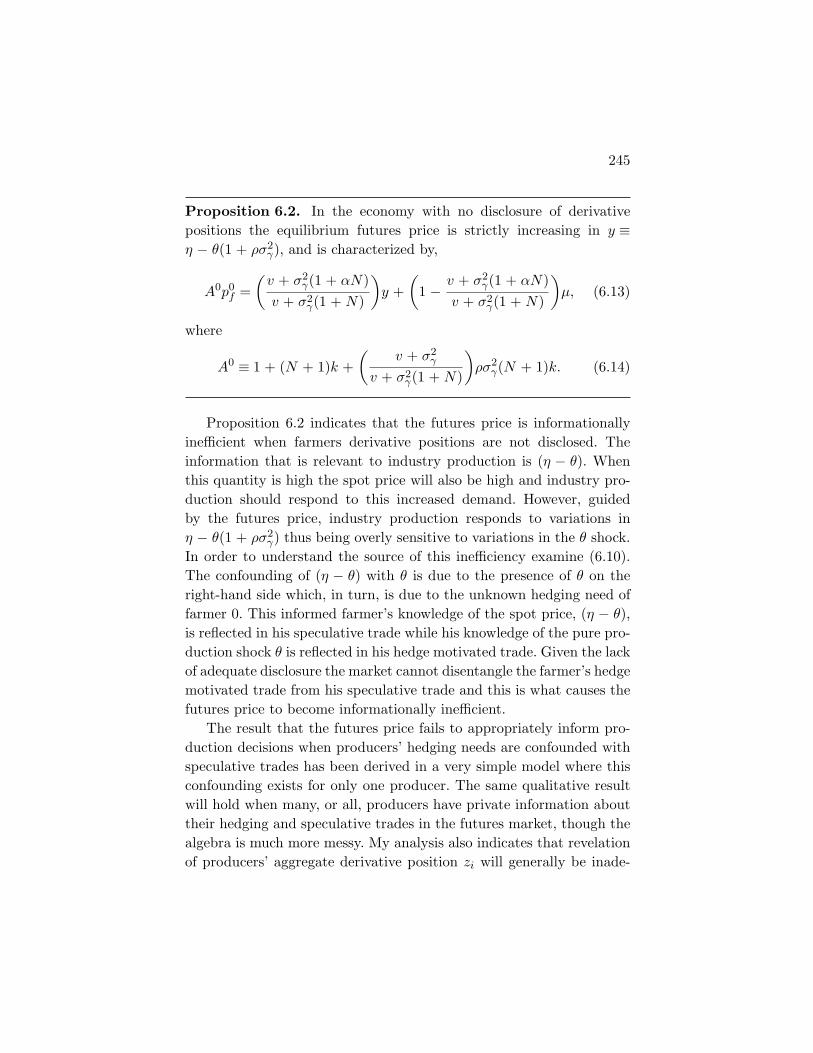
245
Proposition 6.2. In the economy with no disclosure of derivativepositions the equilibrium futures price is strictly increasing in y ≡η − θ(1 + ρσ2
γ), and is characterized by,
A0p0f =
(v + σ2
γ(1 + αN)v + σ2
γ(1 + N)
)y +
(1 − v + σ2
γ(1 + αN)v + σ2
γ(1 + N)
)µ, (6.13)
where
A0 ≡ 1 + (N + 1)k +(
v + σ2γ
v + σ2γ(1 + N)
)ρσ2
γ(N + 1)k. (6.14)
Proposition 6.2 indicates that the futures price is informationallyinefficient when farmers derivative positions are not disclosed. Theinformation that is relevant to industry production is (η − θ). Whenthis quantity is high the spot price will also be high and industry pro-duction should respond to this increased demand. However, guidedby the futures price, industry production responds to variations inη − θ(1 + ρσ2
γ) thus being overly sensitive to variations in the θ shock.In order to understand the source of this inefficiency examine (6.10).The confounding of (η − θ) with θ is due to the presence of θ on theright-hand side which, in turn, is due to the unknown hedging need offarmer 0. This informed farmer’s knowledge of the spot price, (η − θ),is reflected in his speculative trade while his knowledge of the pure pro-duction shock θ is reflected in his hedge motivated trade. Given the lackof adequate disclosure the market cannot disentangle the farmer’s hedgemotivated trade from his speculative trade and this is what causes thefutures price to become informationally inefficient.
The result that the futures price fails to appropriately inform pro-duction decisions when producers’ hedging needs are confounded withspeculative trades has been derived in a very simple model where thisconfounding exists for only one producer. The same qualitative resultwill hold when many, or all, producers have private information abouttheir hedging and speculative trades in the futures market, though thealgebra is much more messy. My analysis also indicates that revelationof producers’ aggregate derivative position zi will generally be inade-

246 Real Effects of Accounting for Derivatives
quate to break this confounding.2 The key additional disclosure neededis disclosure of a producer’s inherent risk, since such disclosure wouldreveal the producer’s hedging needs and therefore allow the speculativecomponent of his derivative trade to be inferred. This implies that fairvalue adjustments to a firm’s derivative position alone is insufficient,but fair value adjustments of both the derivative position as well as theinherent risk that is being hedged (comprehensive fair value account-ing) would fully inform the market.
Additional insights into the inefficiency caused by the lack of ade-quate hedge disclosures is obtained by studying the futures price thatwould obtain if the inherent risk of the informed producer (q0 + θ) aswell as his total derivatives trade z0 is disclosed. I refer to such a regimeas a regime with comprehensive hedge disclosures. Since Proposition 6.1indicates that z0 = (q0 + θ) + E(p|pf ,η,θ)−pf
ρvar(p|pf ,η,θ) , these disclosures reveal
E(p|pf ,η,θ) and therefore reveal the value of (η − θ). Thus, the key infor-mation that was hidden in the regime without hedge disclosures can bereadily inferred without even inverting the equilibrium futures price. Itcan be shown that even if the aggregate derivatives position z0 of theinformed producer is not disclosed but only his inherent risk exposureis disclosed, the same perfect inference of (η − θ) can be made from theequilibrium futures price. Given this inference, all producers have thesame information the market clearing condition becomes:
(N + 1)(
η − θ − Q∗ − p∗f
ρσ2γ
)= Q∗ + θ,
where Q∗ and p∗f denote the equilibrium expected industry produc-
tion and the equilibrium futures price in this fully informed setting.Inserting Q∗ = (N + 1)kp∗
f and solving for p∗f yields:
Proposition 6.3. In the economy with comprehensive hedge disclo-sures the equilibrium futures price is characterized by
A∗p∗f = η − θ − 1
N + 1ρσ2
γθ, (6.15)
2 The information conveyed by a firm’s aggregate derivatives position when its inherent riskis unknown to outsiders is analyzed by Gigler et al. (2007). They show that such partialinformation could lead to rather perverse inferences.

247
where
A∗ ≡ 1 + (N + 1)k +(
1N + 1
)ρσ2
γ(N + 1)k. (6.16)
Having characterized the equilibrium futures price in settings withand without hedge disclosures, we can now examine how the lack ofhedge disclosures impacts industry output. Since in each regime indus-try output is the same multiple of the equilibrium futures price, weneed only examine how the equilibrium futures price differs across thetwo regimes. As one would expect, the equilibrium futures price issometimes higher and sometimes lower in one regime versus the otherdepending on the realizations of η and θ. But, we show that the lack ofhedge disclosures results in a downwards bias to the equilibrium futuresprice and, therefore, in a downwards bias to aggregate industry output.
Proposition 6.4. On average, the equilibrium futures price andthe aggregate industry output is strictly lower in the regime with-out hedge disclosures than in the regime with comprehensive hedgedisclosures.
Proof. The average equilibrium futures price in the regime withouthedge disclosures is obtained by taking the expectation over η and θ inEquation (6.13). Recall that E(y) = E(η − θ(1 + ρσ2
γ)) = µ, so
E(p0f ) =
µ
A0 .
Also, from (6.15),
E(p∗f ) =
µ
A∗
so that E(p∗f ) > E(p0
f ) iff A∗ < A0. Using the expressions for A∗ and A0
given in (6.16) and (6.14) this inequality holds iff N + 1 >v+σ2
γ(N+1)v+σ2
γ,
which is true for all parameter values.
KMSV (2000) show that this downward bias in the futures price iscaused by distortions in risk sharing which, in turn, is caused by the infor-mation asymmetry that exists in equilibriumbetween informed andunin-formed producers. The result described here is very similar to the Easley

248 Real Effects of Accounting for Derivatives
andO’Hara (2004) result onhowthepresenceof informedanduninformedtraders in the capital market drives up a firm’s cost of capital.
In the regime without hedge disclosures, the futures price confoundsfluctuations in (η − θ) with fluctuations in θ. The industry is theninduced to take a “middle of the road” production strategy, under-reacting to one shock and overreacting to the other. It is useful to thinkof (η − θ) and θ as two distinct random variables, where fluctuationsin (η − θ) is equivalent to fluctuations in spot demand and fluctua-tions in θ alone represents shocks to the inherent risk of the informedproducer. Therefore insensitivity of industry output to fluctuations in(η − θ) will have an impact on the volatility of spot prices. If demandis booming, but industry output does not respond adequately to thisbooming demand, the equilibrium spot price will be higher than wouldbe the case if the futures market was fully informed. Conversely whendemand is low and industry output does not adjust downwards in anappropriate manner, equilibrium spot prices will fall disproportionately.The next result proves that is indeed true.
Proposition 6.5. In the regime without hedge disclosures, industryoutput is relatively insensitive to fluctuations in spot market demandand overly sensitive to fluctuations in hedge motivated futures trades.
Proof. From (6.13) the equilibrium futures price in the regime withouthedge disclosures can be expressed as
p0f =
1A0
(v + σ2
γ(1 + αN)v + σ2
γ(1 + N)
)(η − θ − ρσ2
γθ)
+1
A0
(1 − v + σ2
γ(1 + αN)v + σ2
γ(1 + N)
)µ
and, from (6.15), the equilibrium futures price in the regime with com-prehensive hedge disclosures is,
p∗f =
1A∗ (η − θ) − 1
A∗1
N + 1ρσ2
γθ.

249
Since A0 > A∗, as established in Proposition 6.4, and(
v+σ2γ(1+αN)
v+σ2γ(1+N)
)< 1
because α < 1, it follows that the coefficient on (η − θ) is strictlysmaller in the regime without hedge disclosures than in the regime withcomprehensive hedge disclosures, which establishes the first part of theproposition. The second part of the proposition is established by com-paring the coefficients on θ across the two regimes. The claim we needto establish is that 1
A0
(v+σ2
γ(1+αN)v+σ2
γ(1+N)
)ρσ2
γ > 1A∗
1N+1ρσ2
γ , or equivalently,
A∗(
v + σ2γ(1 + αN)
v + σ2γ(1 + N)
)− A0
N + 1> 0.
Substituting the values of A∗ and A0 from (6.16) and (6.14), the claimis equivalent to,
A∗αNσ2γ
v + σ2γ(1 + N)
+(v + σ2
γ)[(1 + (N + 1)k) + ρσ2γk]
v + σ2γ(1 + N)
−1 + (N + 1)k +
(v+σ2
γ
v+σ2γ(1+N)
)ρσ2
γ(N + 1)k
N + 1> 0,
which is equivalent to
A∗αNσ2γ
v + σ2γ(1 + N)
+ [1 + (N + 1)k]
(v + σ2
γ
v + σ2γ(1 + N)
− 1N + 1
)> 0,
which is true since each term on the left-hand side is strictly positive.This completes the proof.
The key result that the absence of hedge disclosures depresses theaggregate output of the industry is missing from the public debatesurrounding SFAS 133. This is not surprising since one would expectindividual firms to be concerned only with their own individual payoffsand not with aggregate phenomena. Our result identifies a very impor-tant externality induced by comprehensive hedge disclosure, that mayactually hurt some individual informed producers, but which shouldbe the proper concern of regulators who choose disclosure standards tomaximize the welfare of the entire community of producers and con-sumers. It would be enormously useful to obtain some empirical esti-mates of the magnitude of the loss in industry output caused by the
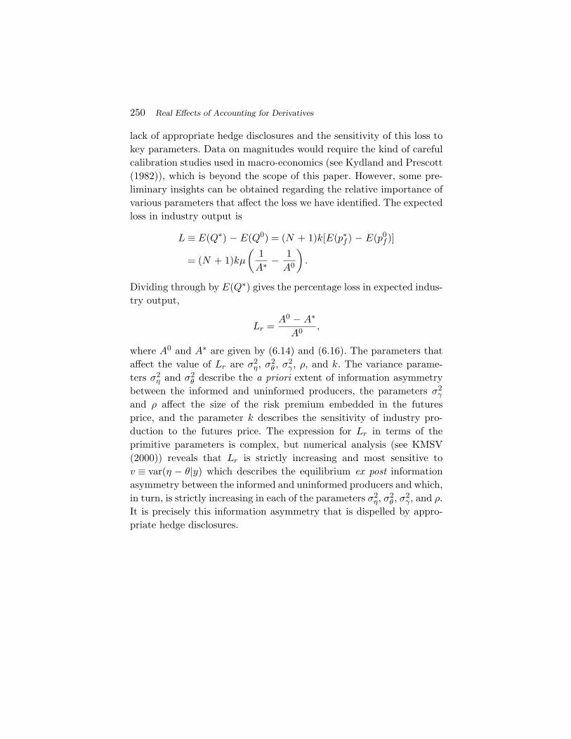
250 Real Effects of Accounting for Derivatives
lack of appropriate hedge disclosures and the sensitivity of this loss tokey parameters. Data on magnitudes would require the kind of carefulcalibration studies used in macro-economics (see Kydland and Prescott(1982)), which is beyond the scope of this paper. However, some pre-liminary insights can be obtained regarding the relative importance ofvarious parameters that affect the loss we have identified. The expectedloss in industry output is
L ≡ E(Q∗) − E(Q0) = (N + 1)k[E(p∗f ) − E(p0
f )]
= (N + 1)kµ
(1
A∗ − 1A0
).
Dividing through by E(Q∗) gives the percentage loss in expected indus-try output,
Lr =A0 − A∗
A0 ,
where A0 and A∗ are given by (6.14) and (6.16). The parameters thataffect the value of Lr are σ2
η, σ2θ , σ2
γ , ρ, and k. The variance parame-ters σ2
η and σ2θ describe the a priori extent of information asymmetry
between the informed and uninformed producers, the parameters σ2γ
and ρ affect the size of the risk premium embedded in the futuresprice, and the parameter k describes the sensitivity of industry pro-duction to the futures price. The expression for Lr in terms of theprimitive parameters is complex, but numerical analysis (see KMSV(2000)) reveals that Lr is strictly increasing and most sensitive tov ≡ var(η − θ|y) which describes the equilibrium ex post informationasymmetry between the informed and uninformed producers and which,in turn, is strictly increasing in each of the parameters σ2
η, σ2θ , σ2
γ , and ρ.It is precisely this information asymmetry that is dispelled by appro-priate hedge disclosures.
7Conclusion
In his survey of the disclosure literature, Verrecchia (2001) calls for a“comprehensive theory of disclosure,” and suggests that such a com-prehensive theory should focus on understanding how a firm’s cost ofcapital is decreased by disclosure that reduces information asymmetryamong traders in the capital market. The real effects perspective, thatI have illustrated, suggests that the key information asymmetry thataffects resource allocation in the economy is the information asymmetrybetween the firm’s managers and the capital market as a whole, ratherthan asymmetries among individual traders in the capital market. Theinformation asymmetry among individual traders does matter, but thiseffect is at most a small second-order effect. Given that firms are, orshould be, focused on value maximization and given that valuation inthe capital market depends critically on what the capital market as awhole knows, I have shown that the information asymmetry betweenmanagers and the capital market could have devastating consequencesfor all stakeholders, informed and uninformed. The consequences ofsuch information asymmetry are masked when disclosure is framed inVerrecchia’s models of pure exchange because the decisions made byfirms are simply absent from the analysis. But they come to life in more
251
252 Conclusion
general equilibrium analysis. It is also obvious that public disclosure byfirms will decrease the kind of information asymmetry I have been dis-cussing as a first-order effect and will reduce information asymmetriesamong individual traders only as a second-order effect.
A real effects perspective suggests that attempts to formulate acomprehensive theory of disclosure would, like a search for the “HolyGrail,” be either futile or sterile. Much more insight can be obtained byfocusing on very specific issues faced by standard setters, such as themeasurement and reporting of derivatives, intangible investments, fairvalues of assets and liabilities, executive stock options, revenue recog-nition criteria, etc. Each of these issues is concerned with informing thecapital market as a whole rather than reducing information asymmetryamong individual traders in the capital market. As demonstrated bythe research surveyed here, each of these issues requires the formula-tion of its own abstraction (model) that is tightly focused on specificmanagerial decisions and each such model requires its own analyticalmethodology and associated empirical analysis. It is unlikely that anygeneral model, that is also analytically tractable, will suffice.

Acknowledgments
I thank Tong Lu, Haresh Sapra, and Raghu Venugopalan for discus-sion, constructive comments, and suggestions that helped improve thispaper.
253
References
Aboody, D. and B. Lev (1998), ‘The value relevance of intangibles: Thecase of software capitalization’. Journal of Accounting Research 36,161–191.
Ball, R. and P. Brown (1968), ‘An empirical evaluation of accountingincome numbers’. Journal of Accounting Research 6, 159–178.
Beaver, W. (1968), ‘The information content of annual earningsannouncements’. Journal of Accounting Research (Supplement) 6,67–92.
Beaver, W. (1972), ‘The behavior of security prices and its implica-tions for accounting research (Methods)’. Supplement to AccountingReview 47, 407–437.
Bhattacharya, S. (1979), ‘Imperfect information, dividend policy, andthe bird in the hand fallacy’. Bell Journal of Economics 10(1), 259–270.
Bowen, R. M., B. Burgstahler, and L. A. Daley (1987), ‘The incrementalinformation content of accrual versus cash flows’. The AccountingReview 62(4), 723–747.
Brandenburger, S. and B. Polak (1996), ‘When managers cover theirposteriors: Making the decisions the market wants to see’. RANDJournal of Economics 27(3), 523–541.
254

References 255
Brock, E. A. (1982), ‘Asset prices in a production economy’. In:J. J. McCall (ed.): The Economics of Information and Uncertainty.Chicago: The University of Chicago Press, pp. 1–43.
Crawford, V. and J. Sobel (1982), ‘Strategic information transmission’.Econometrica 50, 1431–1451.
Danthine, J. P. (1978), ‘Information, futures prices and stabilizing spec-ulation’. Journal of Economic Theory 17, 79–98.
Debreu, G. (1954), ‘Valuation equilibrium and pareto optimum’. Pro-ceedings of National Academy of Science 40, 588–592.
Diamond, D. W. (1985), ‘Optimal release of information by firms’.Journal of Finance 40(4), 1071–1094.
Diamond, D. W. and R. E. Verrecchia (1981), ‘Information aggrega-tion in a noisy rational expectations economy’. Journal of FinancialEconomics 9, 221–235.
Dye, R. A. (1985), ‘Disclosure of nonproprietary information’. Journalof Accounting Research 23, 123–145.
Dye, R. A. (1986), ‘Proprietary and nonproprietary disclosures’. Jour-nal of Business 59, 331–366.
Dye, R. A. (2001), ‘An evaluation of essays on disclosure and the disclo-sure literature in accounting’. Journal of Accounting and Economics32, 181–235.
Easley, D. and M. O’Hara (2004), ‘Information and the cost of capital’.Journal of Finance 59, 1553–1582.
Easton, P., G. Taylor, P. Shroff, and T. Sougiannis (2002), ‘Using fore-casts of earnings to simultaneously estimate growth and the rate ofreturn on equity investment’. Journal of Accounting Research 40(3),657–676.
Feltham, G. and J. Ohlson (1995), ‘Valuation and clean surplusaccounting for operating and financial activities’. ContemporaryAccounting Research 11(2), 689–731.
Gebhardt, W., C. Lee, and B. Swaminathan (2001), ‘Towards an ex-ante cost of capital’. Journal of Accounting Research 39(1), 135–176.
Gigler, F. (1994), ‘Self-enforcing voluntary disclosures’. Journal ofAccounting Research 32, 224–240.
Gigler, F., C. Kanodia, and R. Venugopalan (2007), ‘Assessingthe information content of mark-to-market with mixed attributes:

256 References
The case of cash flow hedges’. Journal of Accounting Research 45(2),257–276.
Gonedes, N. (1976), ‘The capital market, the market for informationand external accounting’. Journal of Finance 31, 611–630.
Graham, K., C. R. Harvey, and S. Rajgopal (2005), ‘The economicimplications of corporate financial reporting’. Journal of Accountingand Economics 40, 3–73.
Grossman, S. J. (1976), ‘On the efficiency of competitive stock marketswhere traders have diverse information’. Journal of Finance 31, 573–585.
Grossman, S. J. (1978), ‘Further results on the informational efficiencyof competitive stock markets’. Journal of Economic Theory 18, 81–101.
Hakannson, N. H., J. Kunkel, and J. Ohlson (1982), ‘Sufficient andnecessary conditions for information to have social value in pureexchange’. Journal of Finance 37, 1169–1181.
Healy, P., S. Myers, and C. Howe (2002), ‘R&D accounting and thetrade-off between relevance and objectivity’. Journal of AccountingResearch 40, 677–710.
Hirshleifer, J. (1971), ‘The private and social value of information andthe reward to inventive activity’. American Economic Review 61,561–574.
Holthausen, R. W. and R. E. Verrecchia (1988), ‘The effect of sequen-tial information releases on the variance of price changes in anintertemporal multi-asset model’. Journal of Accounting Research26, 82–106.
Kanodia, C. (1980), ‘Effects of shareholder information on corporatedecisions and capital market equilibrium’. Econometrica 48(4), 923–953.
Kanodia, C. and D. Lee (1998), ‘Investment and disclosure: The disci-plinary role of periodic performance reports’. Journal of AccountingResearch 36, 33–55.
Kanodia, C. and A. Mukherji (1996), ‘Real effects of separatingoperating and investment cash flows’. Review of AccountingStudies 1, 51–72.

References 257
Kanodia, C., A. Mukherji, H. Sapra, and R.Venugopalan (2000), ‘Hedgedisclosures, futures prices and production distortions’. Journal ofAccounting Research (Supplement) 38, 53–82.
Kanodia, C., H. Sapra, and R.Venugopalan (2004), ‘Should intangi-bles be measured: What are the economic trade-offs?’. Journal ofAccounting Research 42, 89–120.
Kanodia, C., R. Singh, and A. Spero (2005), ‘Imprecision in accountingmeasurement: Can it be value enhancing?’. Journal of AccountingResearch 43(3), 487–519.
Kim, O. and R. E. Verrecchia (1991), ‘Trading volume and price reac-tions to public announcements’. Journal of Accounting Research 29,302–321.
Kydland, F. and E. C. Prescott (1982), ‘Time to build and aggregatefluctuations’. Econometrica 50(6), 1345–1370.
Lambert, R., C. Leuz, and R. E. Verrecchia (2007), ‘Accounting infor-mation, disclosure and the cost of capital’. Journal of AccountingResearch 45(2), 385–420.
Leland, H. and D. Pyle (1977), ‘Information asymmetries, finan-cial structure and financial intermediation’. Journal of Finance 32,371–387.
Lev, B. and T. Sougiannis (1996), ‘The capitalization, amortization,and value relevance of R&D’. Journal of Accounting and Economics21, 107–138.
Lev, B. and P. Zarowin (1999), ‘Boundaries of financial reporting’.Journal of Accounting Research 37, 353–385.
Lucas Jr., R. E. (1978), ‘Asset prices in an exchange economy’. Econo-metrica 46, 1429–1446.
Lucas Jr., R. E. and E. C. Prescott (1971), ‘Investment under uncer-tainty’. Econometrica 39, 659–681.
Melumad, N., G. Weyns, and A. Ziv (1999), ‘Comparing alternativehedge accounting standards: Shareholders’ perspective’. Review ofAccounting Studies 4, 265–292.
Ohlson, J. (1995), ‘Earnings, book values and dividends in equity val-uation’. Contemporary Accounting Research 11(2), 661–687.
Ohlson, J. and G. Gao (2006), ‘Earnings, earnings growth and value’.Foundations and Trends in Accounting 1(1), 1–70.

258 References
Ohlson, J. and B. Juettner-Nauroth (2005), ‘Expected EPS and EPSgrowth as determinants of value’. Review of Accounting Studies 10,349–365.
Ohlson, J. and X. J. Zhang (1999), ‘Accrual accounting and equityvaluation’. Journal of Accounting Research (Supplement) 36, 85–111.
Prescott, E. C. and R. Mehra (1980), ‘Recursive competitive equilib-rium: The case of homogeneous households’. Econometrica 48(6),1365–1379.
Sapra, H. (2001), ‘Do mandatory hedge disclosures discourage orencourage excessive speculation?’. Journal of Accounting Research40(3), 933–964.
Spence, A. M. (1974), ‘Competitive and optimal responses to signals:An analysis of efficiency and distribution’. Journal of Economic The-ory 7, 296–332.
Verrecchia, R. E. (2001), ‘Essays on disclosure’. Journal of Accountingand Economics 32, 97–180.