ACCEPTED VERSION

Sylvan Elhay, Angus R. Simpson, Jochen Deuerlein, Bradley Alexander and Wil H. A. Schilders Reformulated co-tree flows method competitive with the global gradient algorithm for solving water distribution system equations Journal of Water Resources Planning and Management, 2014; OnlinePubl(12):04014040-1-04014040-10 © 2014 American Society of Civil Engineers

http://dx.doi.org/10.1061/(ASCE)WR.1943-5452.0000431

http://hdl.handle.net/2440/84773

PERMISSIONS

http://dx.doi.org/10.1061/9780784479018.ch03

p. 12 – Posting papers on the Internet

Authors may post the final draft of their work on open, unrestricted Internet sites or deposit it in an institutional repository when the draft contains a link to the bibliographic record of the published version in the ASCE Civil Engineering Database. “Final draft” means the version submitted to ASCE after peer review and prior to copyediting or other ASCE production activities; it does not include the copyedited version, the page proof, or a PDF of the published version.

27 January 2015

Reformulated Co-tree flows method competitive with the Global

Gradient Algorithm for solving the water distribution system equations

by

Elhay, S., Simpson, A.R., Deuerlein, J., Alexander, B. and Schilders, W.H.A.

Journal of Water Resources Planning and Management

Citation: Elhay, S., Simpson, A.R., Deuerlein, J., Alexander, B. and Schilders, W.H.A., (2014). “Reformulated Co-tree flows method competitive with the Global Gradient Algorithm for solving the water distribution system equations.” Journal of Water Resources Planning and Management (Corresponding Author Dr. Angus Simpson) Manuscript MS WRENG-1366. Posted ahead of print 9 Jan. 2014. doi: 10.1061/(ASCE)WR.xxxx

For further information about this paper please email Angus Simpson at angus.simpson@adelaide.edu.au

A Reformulated Co-tree Flows Method competitive with the Global

Gradient Algorithm for solving the water distribution system

equations.

Sylvan Elhay1 Angus R. Simpson2 Jochen Deuerlein3 Bradley Alexander4

Wil H.A. Schilders5

December 28, 2013

Abstract1

2

Many different methods have been devised to solve the non-linear systems of equations which3

model water distribution networks. Probably the most popular is the Global Gradient Algorithm4

(GGA) of Todini and Pilati. In the face of the GGA’s success, alternative methods have not aroused5

much interest. One example is the Co-tree method which requires some cumbersome steps in its6

implementation.7

In this paper a Reformulated Co-Trees Method (RCTM) is presented that simplifies the pro-8

cedure by manipulating the incidence matrix into trapezoidal form: a lower triangular block at9

the top representing a spanning tree and rectangular block below it representing the corresponding10

co-tree. This reordering leads to significant efficiencies which make the RCTM competitive with11

the GGA in certain settings.12

The new method has some similarities to the Loop Flows Corrections formulation and it is is13

shown, by application to a set of eight case study networks with between 932 and 19,647 pipes14

and between 848 and 17971 nodes, to be between 15% and 82% faster than the GGA in a setting,15

1Visiting Research Fellow, School of Computer Science, University of Adelaide, South Australia, 5005.2Professor, School of Civil, Environmental and Mining Engineering, University of Adelaide, South Australia, 5005.3Senior Researcher, 3S Consult GmbH, Karlsruhe, Germany & Adjunct Senior Lecturer, School of Civil, Environ-

mental and Mining Engineering, University of Adelaide, South Australia, 5005.4Lecturer, School of Computer Science, University of Adelaide, South Australia, 5005.5Professor, Department of Mathematics and Computer Science, TU Eindhoven, Eindhoven, The Netherlands.

Page: 1

such as optimization using evolutionary algorithms, where the methods are applied hundreds of16

thousands, or even millions, of times to networks with the same topology. It is shown that the key17

matrix for the RCTM can require as little as 7% of the storage requirements of the corresponding18

matrix for the GGA. This can allow for the solution of larger problems by the RCTM than might19

be possible for the GGA in the same computing environment.20

Unlike some alternatives to the GGA, the following features, make the RCTM attractive: (i)21

it does not require a set of initial flows which satisfy continuity, (ii) there is no need to identify22

independent loops or the loops incidence matrix, (iii) a spanning tree and co-tree can be found from23

the incidence matrix without the addition of virtual loops, particularly when multiple reservoirs are24

present, (iv) it does not require the addition of a ground node and pseudo-loops for each demand25

node and does not require the determination of cut-sets.26

In contrast to the GGA, the RCTM does not require special techniques to handle zero flow27

problems which can occur when the head loss is modeled by the Hazen-Williams formula (a sufficient28

condition is given).29

The paper also (i) reports a comparison of the sparsity of the key RCTM and GGA matrices30

for the case study networks, (ii) shows mathematically why the RCTM and GGA always take the31

same number of iterations and produce precisely the same iterates, (iii) establishes that the Loop32

Flows Corrections and the Nullspace methods (previously shown by Nielsen to be equivalent) are33

actually identical to the RCTM.34

35

INTRODUCTION36

A quarter of a century ago Todini & Pilati (1988) introduced the Global Gradient Algorithm37

(GGA) for solving water distribution system (WDS) equations. Almost twenty years later, Todini38

(2006) summarized the popularity of the GGA in comparison to other available approaches when39

he wrote “. . . the practical success of the Global Gradient algorithm as programmed in EPANET 240

(Rossman 2000) leaves no doubts that the easiness of the approach that does not require neither41

a topological analysis aimed at determining the appropriate independent loops nor the need for an42

Page: 2

initial balanced solution, make it the most appropriate fast convergent and robust tool for pipe network43

analysis.”44

The speed with which the GGA executes the Newton iterations has probably contributed most45

to the method’s popularity. The GGA determines the solution of a non-linear system of dimension46

np + nj , where np is the number of pipes and nj is the number of nodes at which the heads are47

unknown, by a two stage iteration in which the linear solver deals with a matrix of dimension only nj .48

This, together with the fact that the matrix to be inverted is sparse and symmetric, leads to a very49

fast algorithm.50

The two points made by Todini about the need for the analysis to find loops and an initial,51

balanced solution were aimed at the Simultaneous Loop Flows Corrections method of Epp & Fowler52

(1970). That method requires the addition of virtual loops when multiple reservoirs are present (a53

process improved by the techniques in the recent paper by Creaco & Franchini (2013)) and some tools54

from graph theory to determine an appropriate set of independent loops. It also requires an initial55

solution which satisfies continuity or mass balance to start the iterative process which determines the56

steady-state solution. However, Todini’s comments refer to parts of the process that are done before57

iteration begins and, while they may be cumbersome, are only done once.58

In a very nice paper Nielsen (1989) showed, among other things, that the Simultaneous Loop59

Flows Corrections method, itself a development of the sequential Loop Flows Corrections method of60

Hardy Cross (1936), is in fact what is called a nullspace method (Benzi, Golub & Liesen 2005). Before61

that, Smith (1982) applied a tree and co-tree method to what is now referred to as the Linear Theory62

Method (Nielsen 1989). In Smith’s method (i) network loops need to be found, (ii) a super-sink63

or ground node needs to be added if there is more than one fixed-head node and (iii) pseudo links64

connecting the fixed head nodes to the ground node need to be added.65

A few years after Nielsen, Rahal (1995) published the Co-Trees Method (CTM). In the CTM, the66

Page: 3

network graph must be transformed into its associated circulating graph, where the network has a67

unique source and each flow is circulating in a pipe from one node to another. This circulating graph68

is formed by adding pseudo-links from each demand node to the main source. A pseudo-link which69

joins each secondary source to the main source is then added. These pseudo-links are required to70

have certain capacities determined by network parameters. Then a spanning tree must be determined71

and the so-called circuit matrix is determined. From it is found a global matrix associated with72

certain cut-sets. The basic equations for the method are then solved using Newton’s method. A set73

of arbitrarily chosen co-tree flows is required to start the method. During the CTM solution process,74

it is necessary to (i) find the associated chain of branches closing a loop for each co-tree chord, and75

(ii) compute pseudo-link head losses.76

It is shown in the present paper, that the CTM of Rahal, which has startup requirements similar77

to those of Smith’s method, is one and the same as the Simultaneous Loop Flows Corrections method.78

The CTM requires the solution at each iterative step of a system of linear equations of dimension79

nc = np − nj , the number of co-tree flows. The number nc is frequently much smaller than nj . As for80

the case of the GGA, the matrix to be inverted in the CTM is symmetric but perhaps because it has81

been thought to be dense, or because of the two criticisms made by Todini, the CTM has not found82

favour and has not been used in practice.83

Nielsen (1989) also suggested permuting the rows of the unknown–head node–arc incidence matrix84

to make its top nj-square block invertible. Twenty years later Schilders (2009), while considering some85

candidates as preconditioners to be used in conjugate gradient solvers for systems similar to WDSs,86

suggested using row and column permutations of the unknown–head node–arc incidence matrix to87

transform it to trapezoidal form, a form in which the top nj × nj block is lower triangular. Now, the88

top nj-square block of such a transformed matrix defines the unknown–head node–arc incidence matrix89

for a spanning tree of the graph of the network and the bottom nc × nj block of the trapezoidal form90

Page: 4

defines the unknown–head node–arc incidence matrix for the corresponding co-tree of the graph of91

the network (Diestel 2010). In the present paper, a new straightforward matrix reduction technique is92

introduced which, when applied to the unknown–head node–arc incidence matrix of the co-tree, leads93

to a reformulation of the Co-Trees Method. Efficiently implemented, The Reformulated Co-Trees94

Method (RCTM) leads to an algorithm that, in many cases, is faster in execution time and requires95

less computer memory than the GGA in settings where many networks with the same topology are96

to be solved.97

The RCTM has the following attractive features:98

(a) it requires neither the use of tools from graph theory to identify independent loops nor does it99

require the addition of virtual loops,100

(b) like the method of Rahal (1995), it does not require an initial solution which satisfies continuity,101

(c) it exhibits greater robustness in the face of zero flows than the GGA which fails catastrophically102

because of the singularity of its key matrix (this failure may be mitigated by the application of103

regularization (Elhay & Simpson 2011)).104

For the eight case study networks studied here, the method (as it would be applied in a genetic or105

Evolutionary Algorithm (EA) optimization)106

(a) has computation time that is between 87% and 55% that of the GGA, and107

(b) has memory requirements that are much smaller than those of the GGA for some networks.108

Item (a) is established by the application of the RCTM to a set of eight case study networks, the109

largest of which has nearly 20,000 pipes.110

Item (b) is established by showing that the storage requirements for the RCTM, although larger111

than that of the GGA for some of the case study networks, is as little as 7% of the GGA requirement112

Page: 5

on other of the case study networks. Thus, in some cases, much larger problems can be solved by113

RCTM than the GGA for the same amount of computer memory.114

The RCTM and the CTM both require the solution of symmetric matrix systems with dimension115

nc. This observation raises the interesting question, not addressed in the present paper, of what116

differences the densities and distributions of the non-zeros in the key matrices of those methods would117

have on the solution times when compared with those of the RCTM. The main interest here, though,118

is a comparison of the GGA and RCTM methods.119

Todini (2006) considered the convergence properties of variations of the GGA and the Simultaneous120

Loop Flow Corrections method numerically and theoretically. Most of the methods considered in that121

paper are derived as linear transformations of the GGA. It is shown empirically there that all the flow-122

based algorithms require the same number of Newton iteration steps to reach exactly the same result123

when applied to certain example problems. In another more recent development, Todini & Rossman124

(2013) have drawn together a unified framework for various algorithms that solve the equations for125

water distribution systems and re-examined their convergence properties.126

In the present paper, the mathematical reason for the fact that the simultaneous loops method and127

the GGAalways, not only take the same number of iterations to converge from the same starting value,128

but produce exactly the same iterates, is explained by deriving the two methods directly from the129

same basic Newton iteration for the steady-state heads and flows that solve the energy and continuity130

equations. It is shown that the Loop Flows Corrections and the Nullspace methods (previously shown131

by Nielsen to be equivalent) are actually mathematically equivalent to the RCTM. Thus, in this paper,132

the three equivalent methods will be referred to as RCTM except where they need to be distinguished.133

The results presented in this paper raise the question of which of the RCTM and GGA methods134

should be chosen in any particular case. A discussion of this question follows the comparison of the135

two methods later in the paper.136

Page: 6

The rest of this paper is structured as follows. Some definitions and notation are introduced137

in the next section. The section following gives the derivation of the method, with some illustrative138

examples interspersed. An algorithmic description of the RCTM is then given, followed by a discussion139

of the relation of the RCTM to other methods. The numerical experiments which support the claims140

about the speed and storage requirements of the method are then presented and they are followed141

by a discussion on choosing which of the methods is most appropriate in a particular case. The142

conclusions section is followed by some appendices which contain material that is necessary for the143

full understanding of the paper but have been moved so as to not disrupt the flow of the exposition.144

145

DEFINITIONS AND NOTATION146

Consider a water distribution network of np pipes, nj(< np) junctions or nodes and nf fixed–head147

nodes. Suppose Qj is the unknown flow for the j-th pipe, pj , which has area of cross section Aj ,148

length Lj , diameter Dj , and resistance factor rj . All the pipes in the system are assumed to have the149

same head loss exponent, n, which is either n = 2 for Darcy–Weisbach head loss model or n = 1.852150

for the Hazen–Williams head loss model. Let Hi denote the unknown head at the i-th node, vi.151

Let q = (Q1, Q2, . . . , Qnp)T denote the vector of unknown flows, h = (H1, H2, . . . ,Hnj )

T denote152

the vector of unknown heads, r = (r1, r2, . . . , rnp)T denote the vector of resistance factors for the pipes,153

d = (d1, d2, . . . , dnj )T denote the vector of nodal demands, and u denote the vector of dimension nf154

of fixed-head elevations.155

The relation between the heads at two ends, node vi and node vk, of a pipe pj and the flow in156

the pipe is defined by Hi − Hk = rjQj |Qj |n−1. Define (i) the square, diagonal matrix G (Todini &157

Pilati 1988) which has elements [G]jj = rj |Qj |n−1, j = 1, 2, . . . , np, (ii) F a diagonal np × np matrix158

in which each diagonal element is the derivative with respect to Q of the element in the corresponding159

row of the vector Gq, (iii) the full column–rank, unknown–head node–arc incidence matrix A1 of160

Page: 7

dimension np × nj , and (iv) the fixed–head, node–arc incidence matrix, A2, of dimension np × nf .161

The steady-state flows and heads in the system are the solutions of the energy and continuity162

equations:163

f(q,h) =

G(q) −A1

−AT1 O

q

h

−A2u

d

= o. (1)

Denote by J the Jacobian of f164

J(q,h) =

F (q) −A1

−AT1 O

.

The Newton iteration for (1) proceeds by taking given starting values q(0), h(0) and repeatedly com-165

puting, for m = 0, 1, 2, . . ., the iterates q(m+1) and h(m+1) from166 F (q(m)) −A1

−AT1 O

q(m+1)

h(m+1)

=

F (q(m))−G(q(m)) o

oT O

q(m)

h(m)

+

A2u

d

(2)

until, if the iteration converges, the difference between successive iterates is sufficiently small. The167

block equations of (2) are, omitting for simplicity the dependency of both F and G on m and q since168

there is no ambiguity169

Fq(m+1) −A1h(m+1) = (F −G)q(m) + A2u, (3)

−AT1 q

(m+1) = d. (4)

170

DERIVATION OF THE REFORMULATED CO-TREES METHOD171

The Schilders (2009) permutations are now applied to the A1 matrix, a step which is essential172

to the derivation of the RCTM. To begin, the spanning tree and co-tree are defined mathematically.173

Suppose Y is a graph. A spanning tree, S, of Y is a subset of the edges of Y that spans every node in174

Y and which is also a tree (Diestel 2010). The co-tree of Y is made up of all the edges in Y which are175

not in S.176

A method is now derived that begins by manipulating the incidence matrix A1 to find matrices,177

T 1 and T 2, which are the unknown–head node-arc incidence matrices of, respectively, a spanning178

Page: 8

tree of the network’s graph and the corresponding co-tree of the network’s graph. From these two179

matrices a reduction of the A1 matrix is derived which leads to a solution of (2) by solving a co-tree180

reformulation of the problem. The method leads to an algorithm during each iterate of which (i) the181

co-tree flows are found and (ii) from them the spanning tree flows are found.182

Recall that nc = np − nj denotes the dimension of the co–tree in the graph of the network. The183

integer nc is also approximately the number of loops in the system. For any unknown–head node-arc184

incidence matrix A1 there exist (Schilders 2009) two (orthogonal) permutation matrices P ∈ Rnp×np185

and R ∈ Rnj×nj and corresponding T 1 ∈ Rnj×nj , lower triangular and T 2 ∈ Rnc×nj which are such186

that187

PA1R =

T 1

T 2

def= T . (5)

A simple proof that the matrix A1 has full rank and an algorithm for the determination of the188

permutations P and R can be found in the Appendix. It is important to note in passing that T 1 is189

invertible because it is a lower triangular matrix with non–zero diagonal elements.190

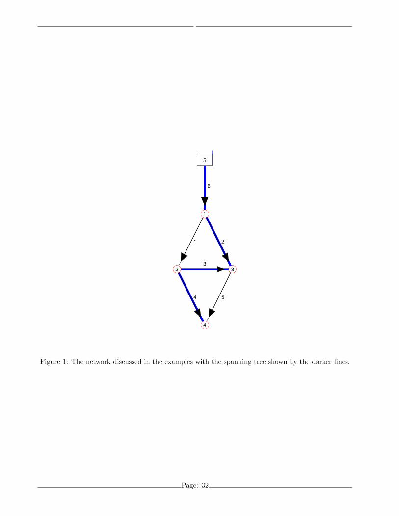
Example 1 Consider the network shown in Figure 1. It has np = 6 pipes, nj = 4 nodes at which the191

head is unknown, and nf = 1 reservoir. The co–tree is comprised of nc = np − nj = 2 pipes. Note192

that if the pipe and node characteristics for this network are symmetric, pipe p3 will have zero flow193

at steady-state. As will be seen, this does not cause a failure of the method, unlike the GGA on the194

same network if the head loss is modeled by the Hazen-Williams formula (Elhay & Simpson 2011).195

The unknown–head node-arc incidence matrix A1 for the network in Figure 1 and the matrices196

T 1,T 2 on the right–hand–side of (5) which result from taking the rows in the order s = (6, 2, 3, 4, 5, 1)197

Page: 9

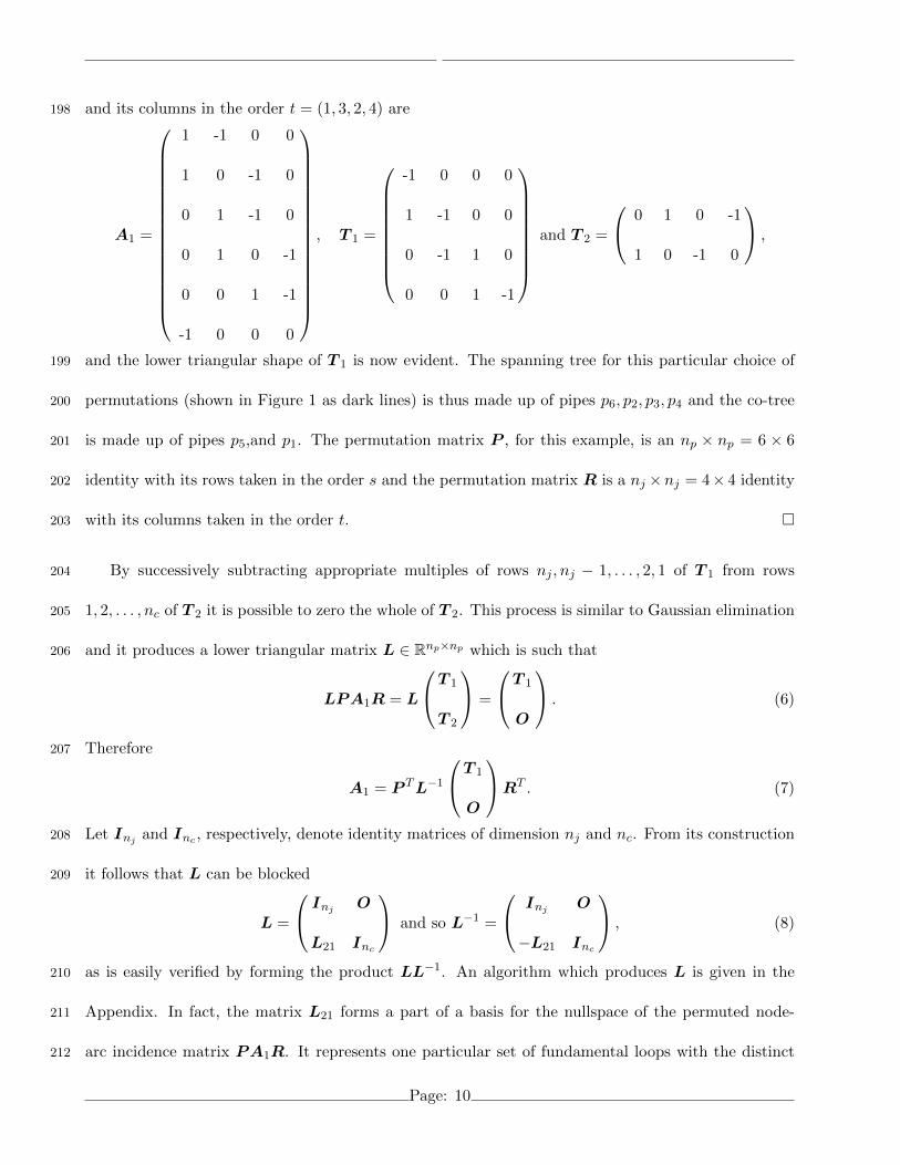
and its columns in the order t = (1, 3, 2, 4) are198

A1 =

1 -1 0 0

1 0 -1 0

0 1 -1 0

0 1 0 -1

0 0 1 -1

-1 0 0 0

, T 1 =

-1 0 0 0

1 -1 0 0

0 -1 1 0

0 0 1 -1

and T 2 =

0 1 0 -1

1 0 -1 0

,

and the lower triangular shape of T 1 is now evident. The spanning tree for this particular choice of199

permutations (shown in Figure 1 as dark lines) is thus made up of pipes p6, p2, p3, p4 and the co-tree200

is made up of pipes p5,and p1. The permutation matrix P , for this example, is an np × np = 6 × 6201

identity with its rows taken in the order s and the permutation matrix R is a nj ×nj = 4× 4 identity202

with its columns taken in the order t. �203

By successively subtracting appropriate multiples of rows nj , nj − 1, . . . , 2, 1 of T 1 from rows204

1, 2, . . . , nc of T 2 it is possible to zero the whole of T 2. This process is similar to Gaussian elimination205

and it produces a lower triangular matrix L ∈ Rnp×np which is such that206

LPA1R = L

T 1

T 2

=

T 1

O

. (6)

Therefore207

A1 = P TL−1

T 1

O

RT . (7)

Let Inj and Inc , respectively, denote identity matrices of dimension nj and nc. From its construction208

it follows that L can be blocked209

L =

Inj O

L21 Inc

and so L−1 =

Inj O

−L21 Inc

, (8)

as is easily verified by forming the product LL−1. An algorithm which produces L is given in the210

Appendix. In fact, the matrix L21 forms a part of a basis for the nullspace of the permuted node-211

arc incidence matrix PA1R. It represents one particular set of fundamental loops with the distinct212

Page: 10

property that every loop has at least one link that is not included in any other loop i.e. such that213

each co-tree link is only in one loop.214

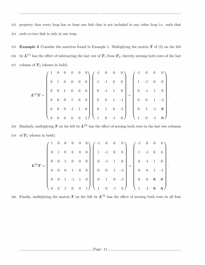
Example 2 Consider the matrices found in Example 1. Multiplying the matrix T of (5) on the left215

by L(1) has the effect of subtracting the last row of T 1 from T 2, thereby zeroing both rows of the last216

column of T 2 (shown in bold).217

L(1)T =

1 0 0 0 0 0

0 1 0 0 0 0

0 0 1 0 0 0

0 0 0 1 0 0

0 0 0 -1 1 0

0 0 0 0 0 1

-1 0 0 0

1 -1 0 0

0 -1 1 0

0 0 1 -1

0 1 0 -1

1 0 -1 0

=

-1 0 0 0

1 -1 0 0

0 -1 1 0

0 0 1 -1

0 1 -1 0

1 0 -1 0

.

Similarly, multiplying T on the left by L(2) has the effect of zeroing both rows in the last two columns218

of T 2 (shown in bold):219

L(2)T =

1 0 0 0 0 0

0 1 0 0 0 0

0 0 1 0 0 0

0 0 0 1 0 0

0 0 1 -1 1 0

0 0 1 0 0 1

-1 0 0 0

1 -1 0 0

0 -1 1 0

0 0 1 -1

0 1 0 -1

1 0 -1 0

=

-1 0 0 0

1 -1 0 0

0 -1 1 0

0 0 1 -1

0 0 0 0

1 -1 0 0

.

Finally, multiplying the matrix T on the left by L(3) has the effect of zeroing both rows in all four220

Page: 11

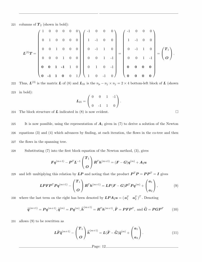
columns of T 2 (shown in bold):221

L(3)T =

1 0 0 0 0 0

0 1 0 0 0 0

0 0 1 0 0 0

0 0 0 1 0 0

0 0 1 -1 1 0

0 -1 1 0 0 1

-1 0 0 0

1 -1 0 0

0 -1 1 0

0 0 1 -1

0 1 0 -1

1 0 -1 0

=

-1 0 0 0

1 -1 0 0

0 -1 1 0

0 0 1 -1

0 0 0 0

0 0 0 0

=

T 1

O

.

Thus, L(3) is the matrix L of (8) and L21 is the np − nj × nj = 2× 4 bottom-left block of L (shown222

in bold):223

L21 =

0 0 1 -1

0 -1 1 0

.

The block structure of L indicated in (8) is now evident. �224

It is now possible, using the representation of A1 given in (7) to derive a solution of the Newton225

equations (3) and (4) which advances by finding, at each iteration, the flows in the co-tree and then226

the flows in the spanning tree.227

Substituting (7) into the first block equation of the Newton method, (3), gives228

Fq(m+1) − P TL−1

T 1

O

RTh(m+1) = (F −G)q(m) + A2u

and left–multiplying this relation by LP and noting that the product P TP = PP T = I gives229

LPFP TPq(m+1) −

T 1

O

RTh(m+1) = LP (F −G)P TPq(m) +

a1

a2

, (9)

where the last term on the right has been denoted by LPA2u = (aT1 aT

2 )T . Denoting230

q(m+1) = Pq(m+1), q(m) = Pq(m), h(m+1)

= RTh(m+1), F = PFP T , and G = PGP T (10)

allows (9) to be rewritten as231

LF q(m+1) −

T 1

O

h(m+1)

= L(F − G)q(m) +

a1

a2

. (11)

Page: 12

Now, let F , G and q(m) be blocked conformally, recalling that F and G are both diagonal, as232

F =

nj nc

nj F 1

nc F 2

, G =

nj nc

nj G1

nc G2

, q(m) =

q(m)1

q(m)2

nj

nc

.

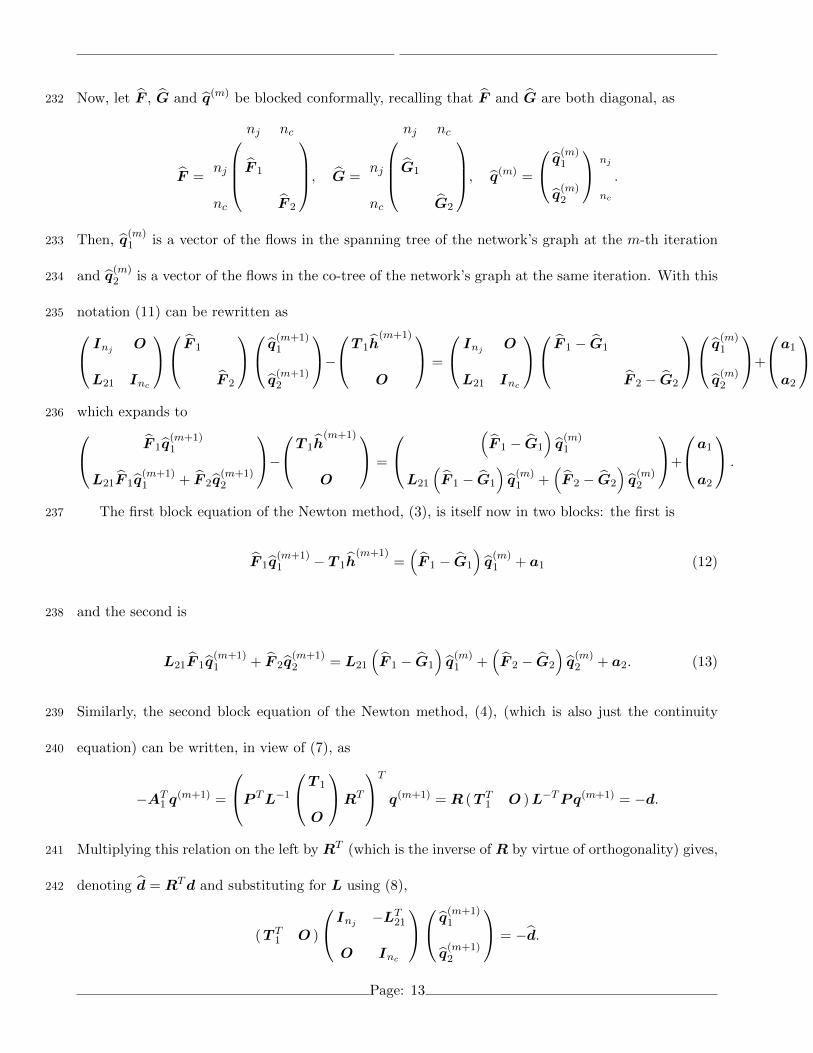
Then, q(m)1 is a vector of the flows in the spanning tree of the network’s graph at the m-th iteration233

and q(m)2 is a vector of the flows in the co-tree of the network’s graph at the same iteration. With this234

notation (11) can be rewritten as235 Inj O

L21 Inc

F 1

F 2

q(m+1)1

q(m+1)2

−T 1h

(m+1)

O

=

Inj O

L21 Inc

F 1 − G1

F 2 − G2

q(m)1

q(m)2

+

a1

a2

which expands to236 F 1q

(m+1)1

L21F 1q(m+1)1 + F 2q

(m+1)2

−T 1h

(m+1)

O

=

(F 1 − G1

)q(m)1

L21

(F 1 − G1

)q(m)1 +

(F 2 − G2

)q(m)2

+

a1

a2

.

The first block equation of the Newton method, (3), is itself now in two blocks: the first is237

F 1q(m+1)1 − T 1h

(m+1)=(F 1 − G1

)q(m)1 + a1 (12)

and the second is238

L21F 1q(m+1)1 + F 2q

(m+1)2 = L21

(F 1 − G1

)q(m)1 +

(F 2 − G2

)q(m)2 + a2. (13)

Similarly, the second block equation of the Newton method, (4), (which is also just the continuity239

equation) can be written, in view of (7), as240

−AT1 q

(m+1) =

P TL−1

T 1

O

RT

T

q(m+1) = R (T T1 O )L−TPq(m+1) = −d.

Multiplying this relation on the left by RT (which is the inverse of R by virtue of orthogonality) gives,241

denoting d = RTd and substituting for L using (8),242

(T T1 O )

Inj −LT21

O Inc

q(m+1)1

q(m+1)2

= −d.

Page: 13

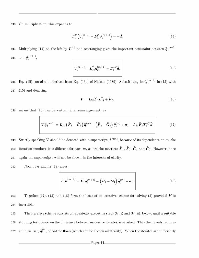
On multiplication, this expands to243

T T1

(q(m+1)1 −LT

21q(m+1)2

)= −d. (14)

Multiplying (14) on the left by T−T1 and rearranging gives the important constraint between q

(m+1)1244

and q(m+1)2 ,245

q(m+1)1 = LT

21q(m+1)2 − T−T

1 d. (15)

Eq. (15) can also be derived from Eq. (13a) of Nielsen (1989). Substituting for q(m+1)1 in (13) with246

(15) and denoting247

V = L21F 1LT21 + F 2, (16)

means that (13) can be written, after rearrangement, as248

V q(m+1)2 = L21

(F 1 − G1

)q(m)1 +

(F 2 − G2

)q(m)2 + a2 + L21F 1T

−T1 d. (17)

Strictly speaking V should be denoted with a superscript, V (m), because of its dependence on m, the249

iteration number: it is different for each m, as are the matrices F 1, F 2, G1 and G2. However, once250

again the superscripts will not be shown in the interests of clarity.251

Now, rearranging (12) gives252

T 1h(m+1)

= F 1q(m+1)1 −

(F 1 − G1

)q(m)1 − a1. (18)

Together (17), (15) and (18) form the basis of an iterative scheme for solving (2) provided V is253

invertible.254

The iterative scheme consists of repeatedly executing steps (b)(i) and (b)(ii), below, until a suitable255

stopping test, based on the difference between successive iterates, is satisfied. The scheme only requires256

an initial set, q(0)2 , of co-tree flows (which can be chosen arbitrarily). When the iterates are sufficiently257

Page: 14

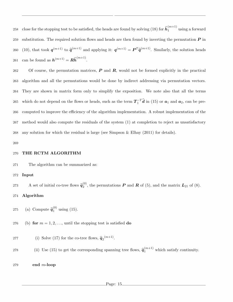
close for the stopping test to be satisfied, the heads are found by solving (18) for h(m+1)

1 using a forward258

substitution. The required solution flows and heads are then found by inverting the permutation P in259

(10), that took q(m+1) to q(m+1) and applying it: q(m+1) = P T q(m+1). Similarly, the solution heads260

can be found as h(m+1) = Rh(m+1)

.261

Of course, the permutation matrices, P and R, would not be formed explicitly in the practical262

algorithm and all the permutations would be done by indirect addressing via permutation vectors.263

They are shown in matrix form only to simplify the exposition. We note also that all the terms264

which do not depend on the flows or heads, such as the term T−T1 d in (15) or a1 and a2, can be pre-265

computed to improve the efficiency of the algorithm implementation. A robust implementation of the266

method would also compute the residuals of the system (1) at completion to reject as unsatisfactory267

any solution for which the residual is large (see Simpson & Elhay (2011) for details).268

269

THE RCTM ALGORITHM270

The algorithm can be summarized as:271

Input272

A set of initial co-tree flows q(0)2 , the permutations P and R of (5), and the matrix L21 of (8).273

Algorithm274

(a) Compute q(0)1 using (15).275

(b) for m = 1, 2, . . ., until the stopping test is satisfied do276

(i) Solve (17) for the co-tree flows, q2(m+1).277

(ii) Use (15) to get the corresponding spanning tree flows, q(m+1)1 which satisfy continuity.278

end m-loop279

Page: 15

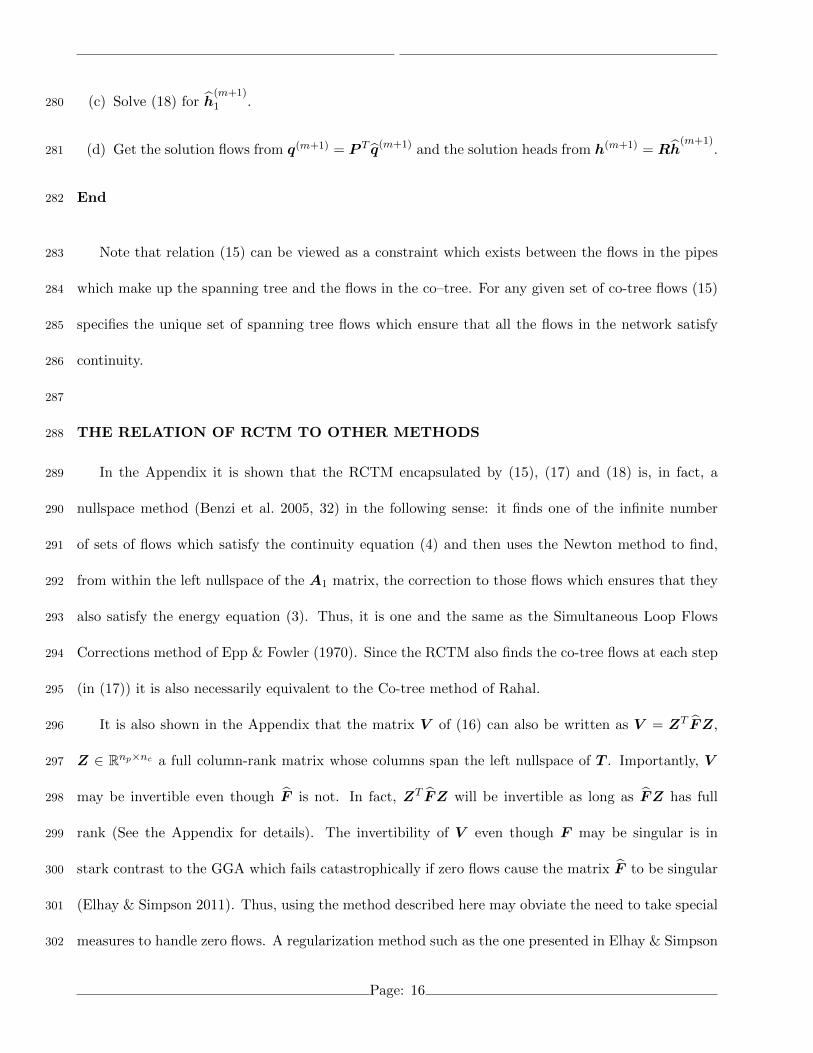
(c) Solve (18) for h(m+1)

1 .280

(d) Get the solution flows from q(m+1) = P T q(m+1) and the solution heads from h(m+1) = Rh(m+1)

.281

End282

Note that relation (15) can be viewed as a constraint which exists between the flows in the pipes283

which make up the spanning tree and the flows in the co–tree. For any given set of co-tree flows (15)284

specifies the unique set of spanning tree flows which ensure that all the flows in the network satisfy285

continuity.286

287

THE RELATION OF RCTM TO OTHER METHODS288

In the Appendix it is shown that the RCTM encapsulated by (15), (17) and (18) is, in fact, a289

nullspace method (Benzi et al. 2005, 32) in the following sense: it finds one of the infinite number290

of sets of flows which satisfy the continuity equation (4) and then uses the Newton method to find,291

from within the left nullspace of the A1 matrix, the correction to those flows which ensures that they292

also satisfy the energy equation (3). Thus, it is one and the same as the Simultaneous Loop Flows293

Corrections method of Epp & Fowler (1970). Since the RCTM also finds the co-tree flows at each step294

(in (17)) it is also necessarily equivalent to the Co-tree method of Rahal.295

It is also shown in the Appendix that the matrix V of (16) can also be written as V = ZT FZ,296

Z ∈ Rnp×nc a full column-rank matrix whose columns span the left nullspace of T . Importantly, V297

may be invertible even though F is not. In fact, ZT FZ will be invertible as long as FZ has full298

rank (See the Appendix for details). The invertibility of V even though F may be singular is in299

stark contrast to the GGA which fails catastrophically if zero flows cause the matrix F to be singular300

(Elhay & Simpson 2011). Thus, using the method described here may obviate the need to take special301

measures to handle zero flows. A regularization method such as the one presented in Elhay & Simpson302

Page: 16

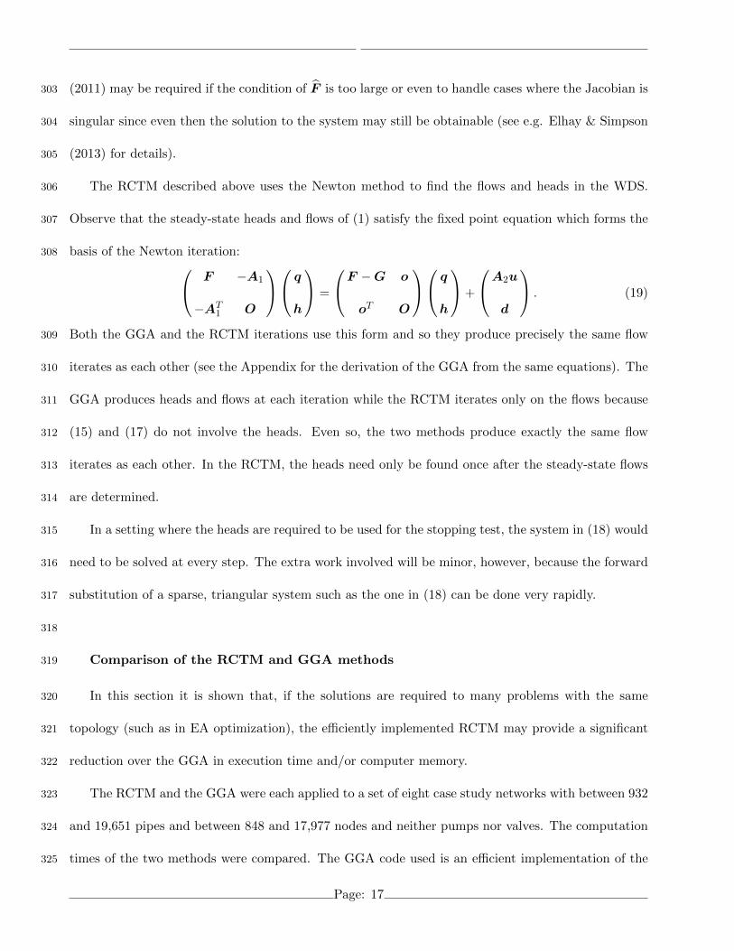
(2011) may be required if the condition of F is too large or even to handle cases where the Jacobian is303

singular since even then the solution to the system may still be obtainable (see e.g. Elhay & Simpson304

(2013) for details).305

The RCTM described above uses the Newton method to find the flows and heads in the WDS.306

Observe that the steady-state heads and flows of (1) satisfy the fixed point equation which forms the307

basis of the Newton iteration:308 F −A1

−AT1 O

q

h

=

F −G o

oT O

q

h

+

A2u

d

. (19)

Both the GGA and the RCTM iterations use this form and so they produce precisely the same flow309

iterates as each other (see the Appendix for the derivation of the GGA from the same equations). The310

GGA produces heads and flows at each iteration while the RCTM iterates only on the flows because311

(15) and (17) do not involve the heads. Even so, the two methods produce exactly the same flow312

iterates as each other. In the RCTM, the heads need only be found once after the steady-state flows313

are determined.314

In a setting where the heads are required to be used for the stopping test, the system in (18) would315

need to be solved at every step. The extra work involved will be minor, however, because the forward316

substitution of a sparse, triangular system such as the one in (18) can be done very rapidly.317

318

Comparison of the RCTM and GGA methods319

In this section it is shown that, if the solutions are required to many problems with the same320

topology (such as in EA optimization), the efficiently implemented RCTM may provide a significant321

reduction over the GGA in execution time and/or computer memory.322

The RCTM and the GGA were each applied to a set of eight case study networks with between 932323

and 19,651 pipes and between 848 and 17,977 nodes and neither pumps nor valves. The computation324

times of the two methods were compared. The GGA code used is an efficient implementation of the325

Page: 17

method described in Simpson & Elhay (2011) and the RCTM code is an efficient implementation326

of the method described in the previous sections of the present paper. Both methods used Matlab327

(Mathworks 2008) sparse arithmetic. The most computationally intensive parts of the two methods328

are (i) the computation of the friction factors (required for F , G, F 1,2 and G1,2 where the head loss is329

modeled by the Darcy-Weisbach formula), (ii) the determination of the permutations P and R and the330

matrix L21, and (iii) the solution of the linear systems with V and W . The rows and columns of these331

key matrices V and W were permuted (just once at the start of each problem) by the Approximate332

Minimum Degree reordering of Amestoy, Davis & Duff (2004). Special C++ codes were devised for333

items (i) and (ii) while the built-in sparse matrix solver in Matlab was used for item (iii). The very334

efficient built-in Matlab solver (\) was used for the two linear systems because, for sparse arguments,335

there is no Cholesky factoring function in Matlab and there are no built-in functions for forward and336

back-substitution. Since the same linear solver was applied to both cases in the comparison, this337

represents a fair test.338

The basic details of the networks considered are given in Table 1 and more detail about them may339

be found in Simpson, Elhay & Alexander (2012). The use of an EA in the design of a network may340

require the determination of the steady-state solutions for hundreds of thousands, or even millions,341

of cases in which all the networks have exactly the same topology but each case has a different set of342

parameters (such as, for example, pipe diameters). It is one purpose of this paper to establish that the343

RCTM, in applications where the solutions are required to many problems with the same topology,344

can be significantly faster than the GGA method and/or can require much less computer memory.345

The speed advantage of the RCTM stems from the fact that (i) the permutations P and R in346

(5), and (ii) the matrix L21 of (14)–(17) need to be determined only once at the start of the design347

process because all the generations of the EA use the same P , R and L21 since the topology remains348

unchanged. Thus, in all the timings that follow the times taken to determine P , R and L21 have been349

Page: 18

excluded from the analysis. It would be necessary, in a one-off calculation using the RCTM, to allow350

the extra time to compute these (which accounts for between 10% and 55% of the total time of the351

RCTM on the case studies presented here).352

In those cases where the RCTM has a memory advantage, it derives from the fact that the key353

matrix which has to be solved at each iteration of the method has fewer non–zero elements.354

355

Timings356

Columns 2–5 of Table 1 show the number, np, of pipes, nj , of nodes, nf , of reservoirs, and, nc, the357

dimension of the co–tree. The next column shows the ratio, as a percentage, of the number of co-tree358

pipes divided by the number of nodes in the network (this number, sometimes called the loop ratio,359

can have an important bearing on the sparsity of matrix factors involved in the solution of the linear360

system. See Piller (1995) for details). The next two columns show the number of non–zero elements361

in the matrices V of (16) and W of (25) and the last column in Table 1 shows the ratio of these362

numbers as a percentage. Of course, the number of non–zeros in V and W for a particular case is363

a function of the spanning tree chosen for that case and different spanning trees could lead to quite364

different matrix sparsities.365

Each method was applied 15 times to each of the case study networks on a single processor PC (the366

calculations were repeated because small variations in the way the operating system runs background367

processes lead to variations in the time taken for the same program to run on the same data). The368

means of the times for solution, τRCTM , τGGA and the means of their ratios τRCTM/τGGA were369

computed. The standard errors of the ratios were also computed and from these the 95% confidence370

intervals for the ratios of the mean times were derived. The mean times for solution, the mean ratios371

of times for solution, and the 95% confidence intervals, I95, are shown in columns 2–5 of Table 2. In372

Table 3 are listed, for illustration, the actual solution times for the RCTM and GGA methods and373

Page: 19

their ratios for the 15 computer runs on Network N1.374

From Table 2 it is evident that the GGA takes between 15% and 82% more time to run than the375

RCTM on the case studies. Clearly, the case in which the RCTM runs in 55% of the time of the GGA,376

on a computation that takes a week justifies the investment required to develop the RCTM program377

code.378

Although it is not the only factor, one important factor which influences the ratio of the compu-379

tation times for the two methods is the number of non–zeros in the matrices V , and W : the more380

non–zeros there are in a matrix, the more computation time will be required to solve a system with381

that matrix if all other thing are equal. But the distribution of the non–zeros within the matrix also382

plays a determining role and this probably explains the deviation from direct proportionality between383

the number of non-zeros and the timings observed in the result reported here.384

It is worth noting that the number of non-zeros in each of the matrices V and W , for the networks385

tested here, is an excellent predictor of the number of non-zeros in its Cholesky factor: the ratio of386

the number of non-zeros in V to the number of non-zeros in its Cholesky factor has an average, for387

the networks tested here, of about 1.8 with standard deviation of .090, so the proportionality between388

them is very close to constant. Similarly, there is an almost 1:1 relationship between the number of389

non-zeros in the matrix V or W and the time taken to solve the linear system efficiently.390

391

Memory requirements392

These numbers shown in columns 7–9 of Table 1 are important because only the non–zero elements393

of a matrix are stored in sparse matrix implementations of matrix solvers such as those used here.394

Thus, the RCTM would require only 7% the storage locations of the GGA for the solution of N5. Of395

course, in some cases, such as N4 and N8 the RCTM has similar or higher storage requirements than396

the GGA. So, it may be possible to solve some problems using the RCTM on a particular machine397

Page: 20

while it is impossible to solve those same problems on the same machine using the GGA because of398

the GGA’s memory requirements.399

A strategy to decide which of the methods to use in a particular case is outlined next.400

401

Choosing between the RCTM and GGA402

The choice between the two methods presented here can be made on any or all of three con-403

siderations: (i) the speed of computation, (ii) the storage requirements or (iii) the presence of zero404

flows.405

In a setting such as network design with an EA it may well be worth investing some effort to406

decide which method is preferable. The matrices V and W can be calculated and the number of407

non–zero elements quickly determined. Prohibitive memory requirements for one method but not the408

other might decide the question. If computer memory is not an issue, then the same problem could409

be solved once by each method and the faster method chosen for the EA solution.410

If the computation times and storage requirements are comparable then the decision might be based411

on the occurrence of zero flows and the possibility that they might occur in some of the variations412

that arise during the optimization. Any significant difference between the two methods, if such exists413

for the problem in question, will help decide the choice.414

415

CONCLUSIONS416

A reformulation which improves the Co-Trees Method, the RCTM, is introduced. The method417

operates by permuting the rows and columns of the incidence matrix to transform it into trapezoidal418

form: a lower triangular block at the top representing a spanning tree and rectangular block below419

it representing the corresponding co-tree. This reordering leads to significant efficiencies which make420

the RCTM competitive with the GGA in certain settings.421

Page: 21

The improved method is shown, by application to a set of eight case study networks with between422

932 and 19,647 pipes and between 848 and 17971 nodes, to take between 55% and 87% of the time423

taken by the GGA to solve the same problems in a setting (e.g. evolutionary algorithms) where the424

methods are applied hundreds of thousands, or even millions, of times to networks with the same425

topology. It is shown that the key matrix for the RCTM can require as little as 7% of the storage426

requirements of the corresponding matrix for the GGA. This can allow for the solution of larger427

problems by the RCTM than might be possible for the GGA in the same computing environment.428

Unlike some alternatives to the GGA, several features, aside from the faster execution time men-429

tioned above, make the RCTM attractive: (i) it does not require a set of initial flows which satisfy430

continuity, (ii) there is no need to identify independent loops or the loops incidence matrix, (iii) a431

spanning tree and co-tree can be found simply from the incidence matrix A1 without the addition432

of virtual loops, particularly when multiple reservoirs are present, (iv) the RCTM does not require433

the addition of a ground node and pseudo-loops or the determination of cut-sets, and (v) exhibits434

greater robustness in the face of zero flows than the GGA which fails catastrophically because of the435

singularity of its key matrices.436

This paper also (i) reports a comparison of the sparsity of the key RCTM and GGA matrices for437

the case study networks, (ii) shows mathematically why the RCTM and GGA always take the same438

number of iterations and produce precisely the same iterates, and (iii) establishes that the RCTM,439

the Loop Flow Corrections Method and the Nullspace Method are one and the same.440

It would be interesting to know if the RCTM applied to pressure-driven simulations can deliver441

similar savings in execution time and/or memory requirements over the GGA applied to those prob-442

lems.443

444

ACKNOWLEDGMENTS445

Page: 22

The authors gratefully thank Prof. Caren Tischendorf for helpful discussions and advice with446

the manuscript. The authors also thank the anonymous reviewers for their helpful and insightful447

comments.448

References449

Amestoy, P. R., Davis, T. A. & Duff, I. (2004), ‘Algorithm 837: AMD, an approximate minimum450

degree ordering algorithm’, ACM Trans. Math. Softw. 30(3), 381–388.451

Benzi, M., Golub, G. & Liesen, J. (2005), ‘Numerical solution of saddle point problems’, Acta. Num.452

pp. 1–137.453

Creaco, E. & Franchini, M. (2013), ‘Comparison of newton-raphson global and loop algorithms454

for water distribution network resolution’, J. Hydraul. Eng. . Posted ahead of print. DOI:455

10.1061/(ASCE)HY.1943-7900.0000825.456

Cross, H. (1936), ‘Analysis of flow in networks of conduits or conductors’, Bulletin, The University of457

Illinois Eng. Experiment Station 286.458

Diestel, R. (2010), Graph Theory, Vol. 173 of Graduate texts in mathematics, fourth edn, Spriger-459

Verlag, Heidelberg.460

Elhay, S. & Simpson, A. (2011), ‘Dealing with zero flows in solving the non–linear equa-461

tions for water distribution systems’, Journal of Hydraulic Engineering 137(10), 1216–1224.462

doi:10.1061/(ASCE)HY.1943-7900.0000411. ISSN: 0733-9429.463

Elhay, S. & Simpson, A. (2013), ‘Closure on ”dealing with zero flows in solving the non-linear equa-464

tions for water distribution systems”’, Journal of Hydraulic Engineering 139(5), 560–562. DOI:465

10.1061/(ASCE)HY.1943-7900.0000696.466

Page: 23

Epp, R. & Fowler, A. (1970), ‘Efficient code for steady-state flows in networks’, Journal of the Hy-467

draulics Division, Proceedings of the ASCE 96(HY1), 43–56.468

Mathworks, T. (2008), Using Matlab, The Mathworks Inc., Natick, MA.469

Nielsen, H. (1989), ‘Methods for analyzing pipe networks’, J. Hydraul. Eng. 115(2), 139–157.470

Piller, O. (1995), Modeling the behavior of a network - Hydraulic analysis and a sampling procedure471

for estimating the parameters., PhD thesis, University of Bordeaux, France. Ph.D. Thesis, in472

French.473

Rahal, H. (1995), ‘A co–tree formulation for steady state in water distribution networks’, Advances in474

Engineering Software 22(3), 169–178.475

Rossman, L. (2000), EPANET 2 Users Manual, Water Supply and Water Resources Division, National476

Risk Management Research Laboratory, Cincinnati, OH45268.477

Schilders, W. (2009), ‘Solution of indefinite linear systems using an LQ decomposition for the linear478

constraints’, Linear Algebra Appl. 431, 381–395.479

Simpson, A. & Elhay, S. (2011), ‘The Jacobian for solving water distribution system equations480

with the Darcy-Weisbach head loss model’, Journal of Hydraulic Engineering 137(6), 696–700.481

doi:10.1061/(ASCE)HY.1943-7900.0000341. ISSN: 0733-9429.482

Simpson, A., Elhay, S. & Alexander, B. (2012), ‘A forestcore partitioning algorithm for speeding up483

the analysis of water distribution systems’, J. Water Resour. Plann. Manage. . Accepted and484

posted online Nov. 21, 2012. DOI: 10.1061/(ASCE)WR.1943-5452.0000336.485

Smith, A. (1982), ‘Compact formulation of pipe network problems’, Can. J. Civ. Eng. 9, 611–623.486

Page: 24

Todini, E. (2006), On the convergence properties of the different pipe network algorithms, in ‘Pro-487

ceedings of the 8th Annual Water Distribution Systems Analysis Symposium’, Cincinnati, Ohio,488

USA, pp. 1–16.489

Todini, E. & Pilati, S. (1988), A gradient algorithm for the analysis of pipe networks., John Wiley and490

Sons, London, pp. 1–20. B. Coulbeck and O. Chun-Hou (eds).491

Todini, E. & Rossman, L. (2013), ‘Unified framework for deriving simultaneous equation algorithms492

for water distribution networks.’, J. Hydraul. Eng. 139(5), 511–526.493

Page: 25

APPENDICES494

495

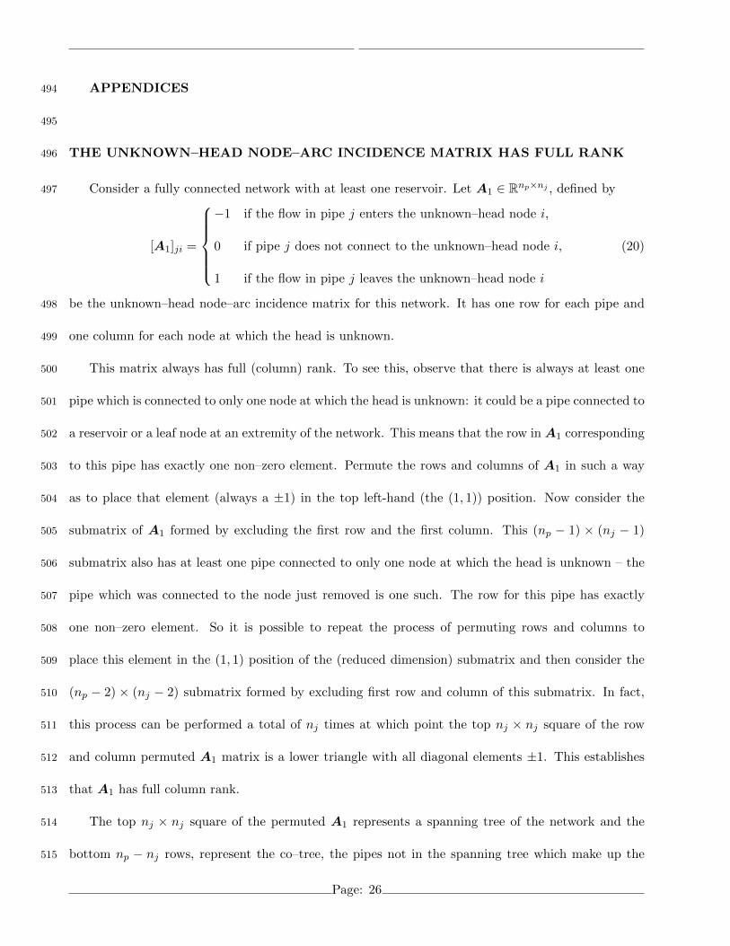
THE UNKNOWN–HEAD NODE–ARC INCIDENCE MATRIX HAS FULL RANK496

Consider a fully connected network with at least one reservoir. Let A1 ∈ Rnp×nj , defined by497

[A1]ji =

−1 if the flow in pipe j enters the unknown–head node i,

0 if pipe j does not connect to the unknown–head node i,

1 if the flow in pipe j leaves the unknown–head node i

(20)

be the unknown–head node–arc incidence matrix for this network. It has one row for each pipe and498

one column for each node at which the head is unknown.499

This matrix always has full (column) rank. To see this, observe that there is always at least one500

pipe which is connected to only one node at which the head is unknown: it could be a pipe connected to501

a reservoir or a leaf node at an extremity of the network. This means that the row in A1 corresponding502

to this pipe has exactly one non–zero element. Permute the rows and columns of A1 in such a way503

as to place that element (always a ±1) in the top left-hand (the (1, 1)) position. Now consider the504

submatrix of A1 formed by excluding the first row and the first column. This (np − 1) × (nj − 1)505

submatrix also has at least one pipe connected to only one node at which the head is unknown – the506

pipe which was connected to the node just removed is one such. The row for this pipe has exactly507

one non–zero element. So it is possible to repeat the process of permuting rows and columns to508

place this element in the (1, 1) position of the (reduced dimension) submatrix and then consider the509

(np − 2) × (nj − 2) submatrix formed by excluding first row and column of this submatrix. In fact,510

this process can be performed a total of nj times at which point the top nj × nj square of the row511

and column permuted A1 matrix is a lower triangle with all diagonal elements ±1. This establishes512

that A1 has full column rank.513

The top nj × nj square of the permuted A1 represents a spanning tree of the network and the514

bottom np − nj rows, represent the co–tree, the pipes not in the spanning tree which make up the515

Page: 26

network loops.516

517

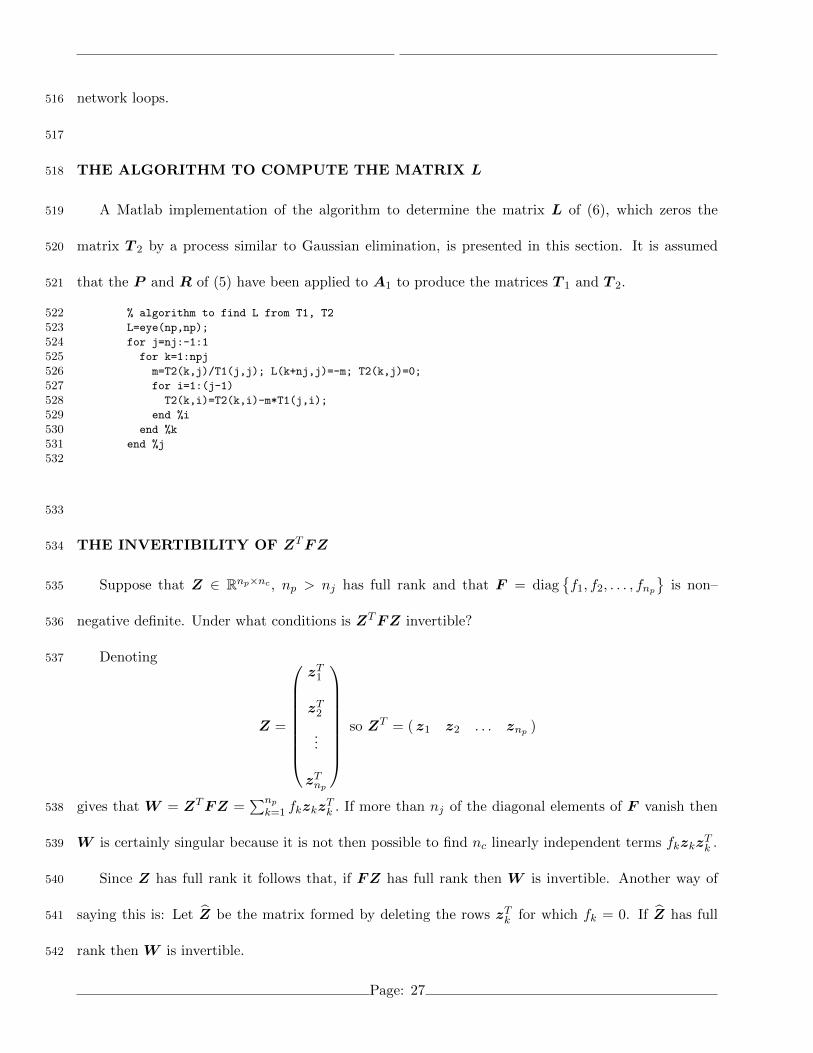
THE ALGORITHM TO COMPUTE THE MATRIX L518

A Matlab implementation of the algorithm to determine the matrix L of (6), which zeros the519

matrix T 2 by a process similar to Gaussian elimination, is presented in this section. It is assumed520

that the P and R of (5) have been applied to A1 to produce the matrices T 1 and T 2.521

% algorithm to find L from T1, T2522L=eye(np,np);523for j=nj:-1:1524

for k=1:npj525m=T2(k,j)/T1(j,j); L(k+nj,j)=-m; T2(k,j)=0;526for i=1:(j-1)527

T2(k,i)=T2(k,i)-m*T1(j,i);528end %i529

end %k530end %j531

532

533

THE INVERTIBILITY OF ZTFZ534

Suppose that Z ∈ Rnp×nc , np > nj has full rank and that F = diag{f1, f2, . . . , fnp

}is non–535

negative definite. Under what conditions is ZTFZ invertible?536

Denoting537

Z =

zT1

zT2

...

zTnp

so ZT = (z1 z2 . . . znp )

gives that W = ZTFZ =∑np

k=1 fkzkzTk . If more than nj of the diagonal elements of F vanish then538

W is certainly singular because it is not then possible to find nc linearly independent terms fkzkzTk .539

Since Z has full rank it follows that, if FZ has full rank then W is invertible. Another way of540

saying this is: Let Z be the matrix formed by deleting the rows zTk for which fk = 0. If Z has full541

rank then W is invertible.542

Page: 27

543

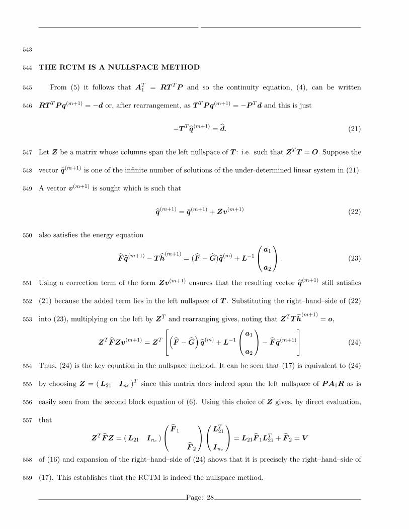
THE RCTM IS A NULLSPACE METHOD544

From (5) it follows that AT1 = RT TP and so the continuity equation, (4), can be written545

RT TPq(m+1) = −d or, after rearrangement, as T TPq(m+1) = −P Td and this is just546

−T T q(m+1) = d. (21)

Let Z be a matrix whose columns span the left nullspace of T : i.e. such that ZTT = O. Suppose the547

vector q(m+1) is one of the infinite number of solutions of the under-determined linear system in (21).548

A vector v(m+1) is sought which is such that549

q(m+1) = q(m+1) + Zv(m+1) (22)

also satisfies the energy equation550

F q(m+1) − T h(m+1)

= (F − G)q(m) + L−1

a1

a2

. (23)

Using a correction term of the form Zv(m+1) ensures that the resulting vector q(m+1) still satisfies551

(21) because the added term lies in the left nullspace of T . Substituting the right–hand–side of (22)552

into (23), multiplying on the left by ZT and rearranging gives, noting that ZTT h(m+1)

= o,553

ZT FZv(m+1) = ZT

(F − G)q(m) + L−1

a1

a2

− F q(m+1)

(24)

Thus, (24) is the key equation in the nullspace method. It can be seen that (17) is equivalent to (24)554

by choosing Z = (L21 Inc )T since this matrix does indeed span the left nullspace of PA1R as is555

easily seen from the second block equation of (6). Using this choice of Z gives, by direct evaluation,556

that557

ZT FZ = (L21 Inc )

F 1

F 2

LT21

Inc

= L21F 1LT21 + F 2 = V

of (16) and expansion of the right–hand–side of (24) shows that it is precisely the right–hand–side of558

(17). This establishes that the RCTM is indeed the nullspace method.559

Page: 28

560

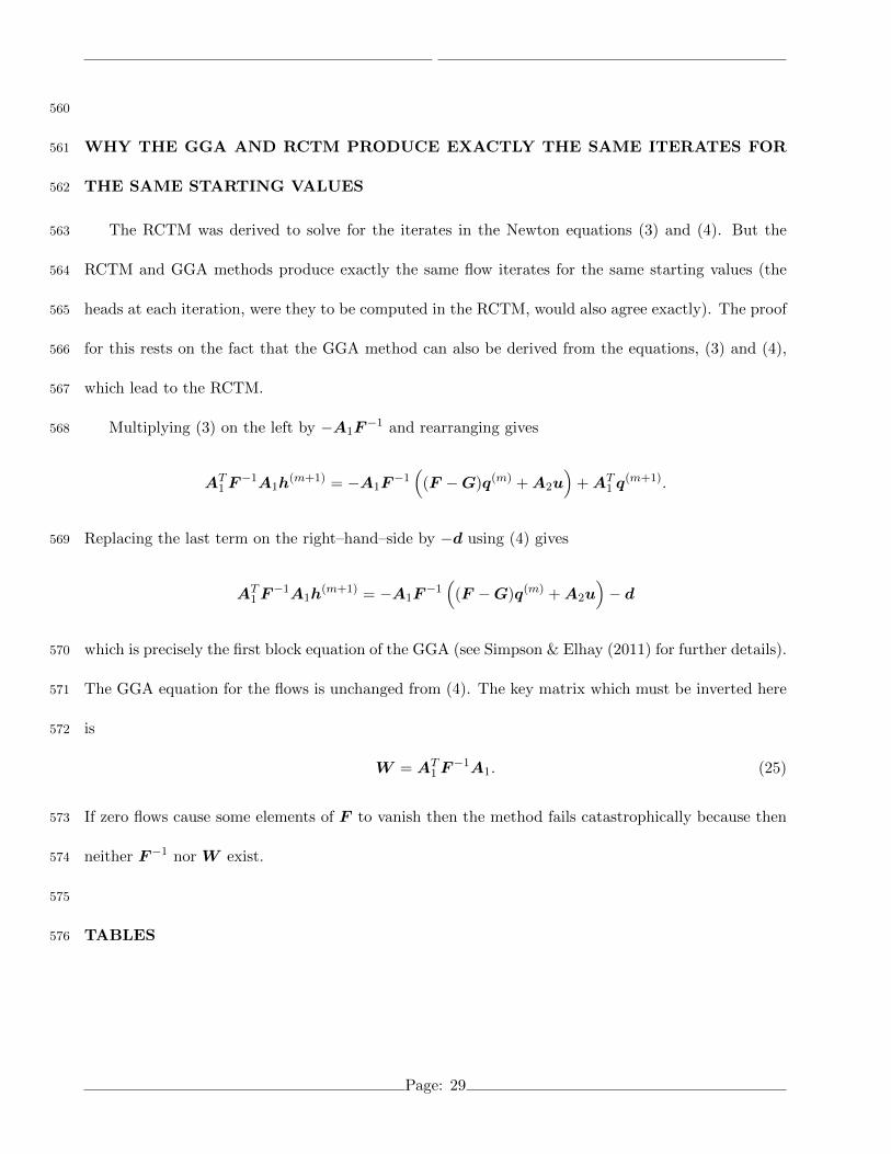
WHY THE GGA AND RCTM PRODUCE EXACTLY THE SAME ITERATES FOR561

THE SAME STARTING VALUES562

The RCTM was derived to solve for the iterates in the Newton equations (3) and (4). But the563

RCTM and GGA methods produce exactly the same flow iterates for the same starting values (the564

heads at each iteration, were they to be computed in the RCTM, would also agree exactly). The proof565

for this rests on the fact that the GGA method can also be derived from the equations, (3) and (4),566

which lead to the RCTM.567

Multiplying (3) on the left by −A1F−1 and rearranging gives568

AT1 F

−1A1h(m+1) = −A1F

−1(

(F −G)q(m) + A2u)

+ AT1 q

(m+1).

Replacing the last term on the right–hand–side by −d using (4) gives569

AT1 F

−1A1h(m+1) = −A1F

−1(

(F −G)q(m) + A2u)− d

which is precisely the first block equation of the GGA (see Simpson & Elhay (2011) for further details).570

The GGA equation for the flows is unchanged from (4). The key matrix which must be inverted here571

is572

W = AT1 F

−1A1. (25)

If zero flows cause some elements of F to vanish then the method fails catastrophically because then573

neither F−1 nor W exist.574

575

TABLES576

Page: 29

ID np nj nf ncncnj

% nnz(V ) nnz(W ) nnz(V )

nnz(W )%

N1 932 848 8 84 10% 350 2682 13%

N2 1118 1039 2 79 8% 1141 3265 35%

N3 1975 1770 4 205 12% 2491 5706 44%

N4 2465 1890 3 575 30% 6855 6714 102%

N5 2509 2443 2 66 3% 534 7451 7%

N6 8585 8392 2 193 2% 2633 25554 10%

N7 14830 12523 7 2307 18% 31601 41147 77%

N8 19647 17971 15 1676 9% 70942 57233 124%

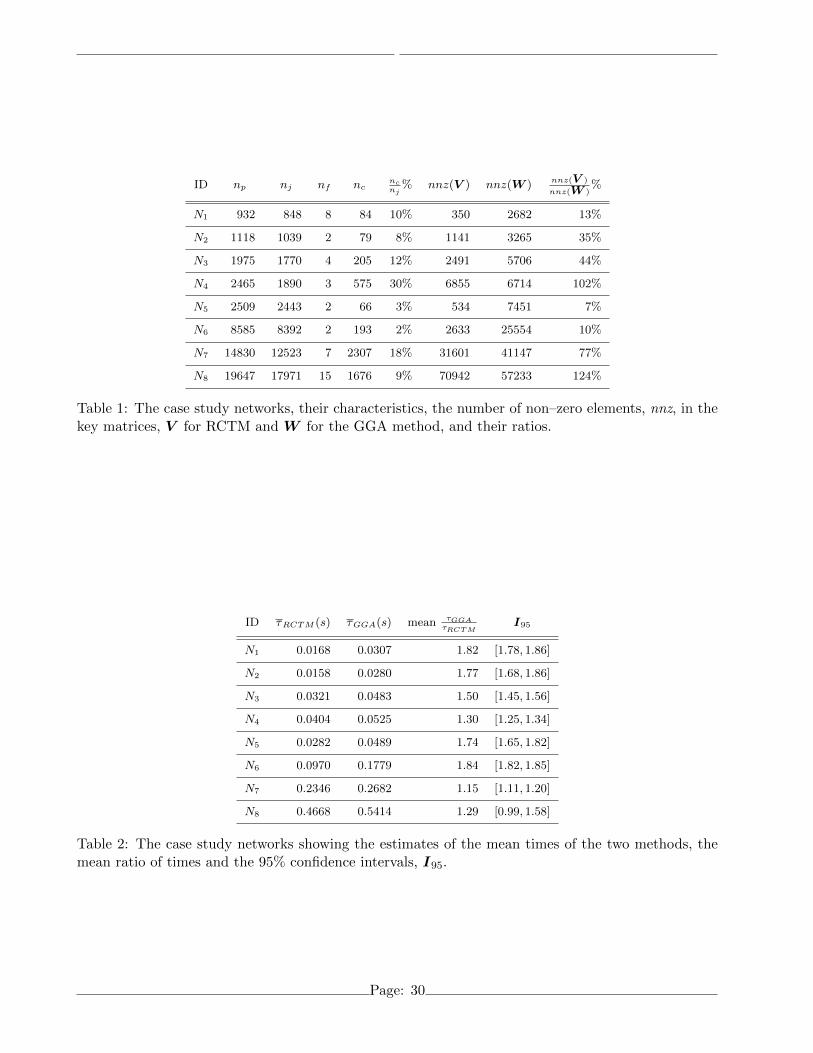
Table 1: The case study networks, their characteristics, the number of non–zero elements, nnz, in thekey matrices, V for RCTM and W for the GGA method, and their ratios.

ID τRCTM (s) τGGA(s) mean τGGAτRCTM

I95

N1 0.0168 0.0307 1.82 [1.78, 1.86]

N2 0.0158 0.0280 1.77 [1.68, 1.86]

N3 0.0321 0.0483 1.50 [1.45, 1.56]

N4 0.0404 0.0525 1.30 [1.25, 1.34]

N5 0.0282 0.0489 1.74 [1.65, 1.82]

N6 0.0970 0.1779 1.84 [1.82, 1.85]

N7 0.2346 0.2682 1.15 [1.11, 1.20]

N8 0.4668 0.5414 1.29 [0.99, 1.58]

Table 2: The case study networks showing the estimates of the mean times of the two methods, themean ratio of times and the 95% confidence intervals, I95.

Page: 30

tRCTM (s) tGGA(s)tGGAtRCTM

0.0196 0.0349 1.78

0.0166 0.0293 1.76

0.0166 0.0292 1.76

0.0166 0.0293 1.77

0.0166 0.0295 1.78

0.0167 0.0294 1.76

0.0171 0.0295 1.73

0.0166 0.0306 1.84

0.0166 0.0298 1.80

0.0166 0.0297 1.79

0.0166 0.0319 1.92

0.0166 0.0316 1.90

0.0166 0.0311 1.88

0.0166 0.0327 1.97

0.0166 0.0316 1.90

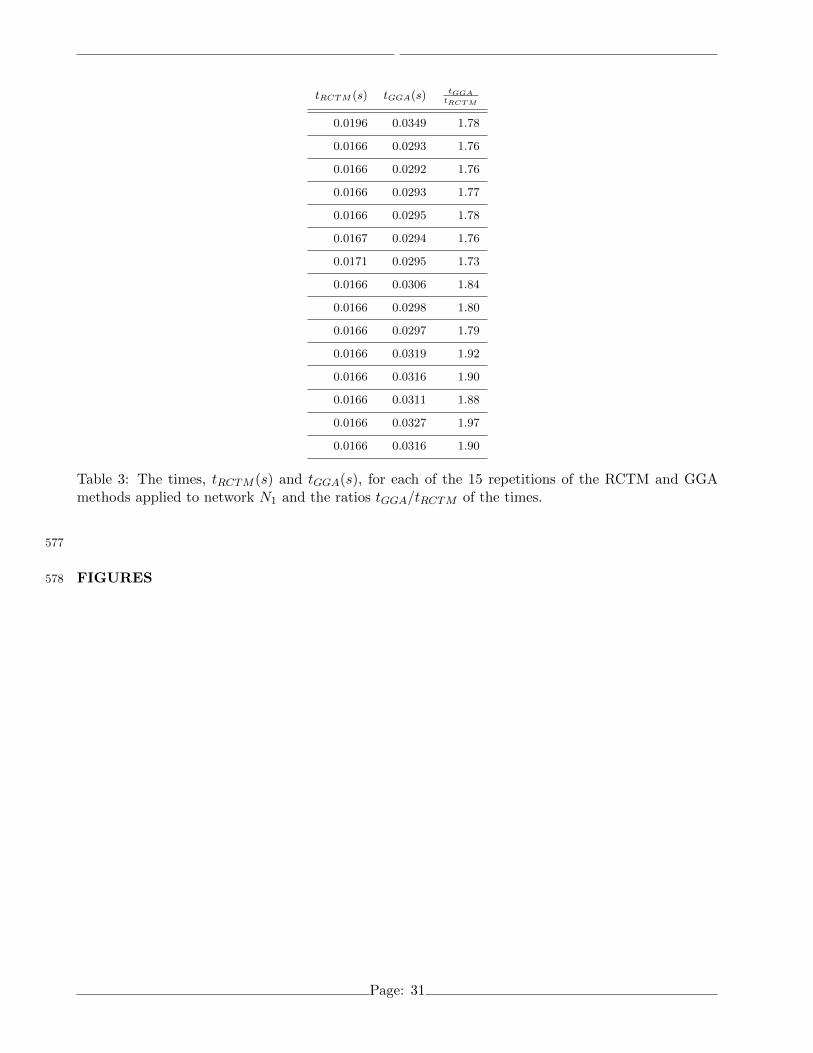
Table 3: The times, tRCTM (s) and tGGA(s), for each of the 15 repetitions of the RCTM and GGAmethods applied to network N1 and the ratios tGGA/tRCTM of the times.

577

FIGURES578

Page: 31

1 2

3

4 5

6

1

2 3

4

5

Figure 1: The network discussed in the examples with the spanning tree shown by the darker lines.

Page: 32

List of Figures579

1 The network discussed in the examples with the spanning tree shown by the darker lines. 32580

List of Tables581

1 The case study networks, their characteristics, the number of non–zero elements, nnz,582

in the key matrices, V for RCTM and W for the GGA method, and their ratios. . . . 30583

2 The case study networks showing the estimates of the mean times of the two methods,584

the mean ratio of times and the 95% confidence intervals, I95. . . . . . . . . . . . . . . 30585

3 The times, tRCTM (s) and tGGA(s), for each of the 15 repetitions of the RCTM and586

GGA methods applied to network N1 and the ratios tGGA/tRCTM of the times. . . . . 31587

Page: 33