AC 2007-78: A STUDENT PROJECT ON AIRFOIL PERFORMANCE

John Matsson, Oral Roberts UniversityO. JOHN E. MATSSON is an Associate Professor of Mechanical Engineering at Oral RobertsUniversity in Tulsa, Oklahoma. He earned M.S. and Ph.D. degrees from the Royal Institute ofTechnology in Stockholm, Sweden in 1988 and 1994, respectively.

© American Society for Engineering Education, 2007

A Student Project on Airfoil Performance

Abstract

This paper shows a course project in an undergraduate engineering program with a mechanical emphasis. The students used LabVIEW software for measurements of the pressure distribution on the surface of a Clark-Y airfoil at different angles of attack in a low-speed wind tunnel. Both the wind tunnel speed and the angle of attack of the airfoil were automatically controlled from the software. Furthermore, the LabVIEW software also controlled the Scanivalve solenoid for pressure measurements. The experiments were compared with computations using the CosmosFloWorks software.

Introduction

The experimental set up described in this paper is used for demonstrations and labs in the introduction to engineering, fluid mechanics and experimental methods courses at ORU. In the introduction to engineering course the students are introduced to aerodynamics and the airfoil setup is used as a demonstration of the capabilities of LabVIEW software to measure the pressure distribution and calculate lift forces on an airfoil. In the experimental methods course the students learn to use LabVIEW and the Clark-Y set up is therefore used as a lab where the students see an application of LabVIEW for both stepper motor control and measurements. In the fluid mechanics course the lab is more directed towards obtaining the lift coefficient curves for different Reynolds numbers and angles of attack. Furthermore, the intention is also in the future to include measurements of the boundary layer on the airfoil and the wake region downstream of the trailing edge using a Pitot tube and hot-wire anemometry. While it is true that airfoil experiments have been in existence for many years and are manufactured by different companies, it is to the author’s knowledge the first time that pressure distribution measurements have been integrated with stepper motor control of the angle of attack using LabVIEW software. The learning objective has been for the students to get the experience of working together as a design group towards the completion of a specified task that includes the use of their knowledge gained in different courses.

Junior and senior students in the fluid mechanics course designed the experimental setup for pressure measurements around the airfoil. The reason for the selection of this project in this course was to increase student learning by incorporating a lab on airfoil performance which is part of the course curriculum. It is also motivating for the students to work on a project that designs, builds and tests an experimental set up that is later used in different labs and demonstrations by other students during many years. Three of the students worked on the airfoil and stepper motor assembly design while three other students contributed to the wind tunnel speed control portion using LabVIEW programming. Some of the students had individual assignments related to the project as for example one student worked on the stepper motor assembly and fabrication. Two other students worked together as a team on the electronics part of the project by soldering relays and other components that they mounted in a project box and connected to the A/D board and the Scanivalve. At the department we are also fortunate to have

a skillful technician that helped the students on the project by working on the Clark-Y airfoil assembly. The Clark-Y airfoil is named after Col. Virginius E. Clark, who designed the airfoil in 1922. This airfoil with its characteristic flat lower surface has frequently been used in different applications ranging from propellers to sailplane wings. One of the first measurements of pressure distributions on this airfoil were done by Jacobs et. al

1, followed by Marchman and Werme2 and Stern et. al

3 that made low Reynolds number measurements. Warner4 also have included results

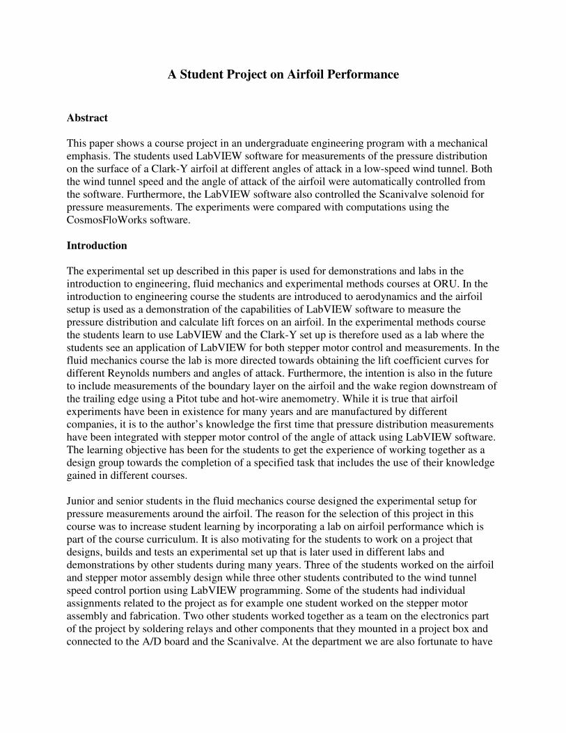
from tests of the Clark-Y airfoil. The angle of attack of the airfoil could be varied using a Hurst Series AS 3004-001, ABS geared stepping motor5 that was controlled by a NI PCI-6040E A/D board6 connected to a NI BNC-2110 Shielded Connector Block7 with Digital I/O and a Modern Technology MTSD-V1-ND Unipolar Stepper Motor Driver Board8. The LabVIEW software9 was also used to control a Scanivalve CTLR2P-S2-S6 Solenoid Controller with Pulser10 connected to two W1266/1P-24T Fluid Switch Wafers for pressure measurements. The non-tapered and non-swept Clark-Y wing section has a chord length of 0.152 m, a maximum thickness of 0.0238 m, and a span of 0.3m. The dimensions of the wind tunnel cross section were 0.3m x 0.3m and the length of the test section was 1.0 m. The wing section has a middle part made of aluminum sandwiched in between two polished pieces of wood, see Figure 1. The figure shows the Hurst stepper motor connected to the airfoil with an aluminum tube that contains half of the pressure lines. The remaining pressure lines were guided through the wind tunnel wall at the opposite side of the stepper motor. The Pitot tube located above the airfoil was used to measure the free stream velocity in the wind tunnel.

Figure 1. Clark-Y airfoil and stepper motor assembly. A Pitot tube is also shown above the airfoil. The coordinates of the Clark-Y airfoil are shown in Table 1, see also Riegels11 and Mason12. Thirty pressure fittings were connected to the middle section and Tygon tubing was connected to each pressure tap. The pressure holes were located on both the lower and upper surfaces at the following chord-wise positions: x/c = 0, 0.0125, 0.025, 0.05, 0.075, 0.1, 0.15, 0.2, 0.3, 0.4, 0.5,

0.6, 0.7, 0.8, 0.87.

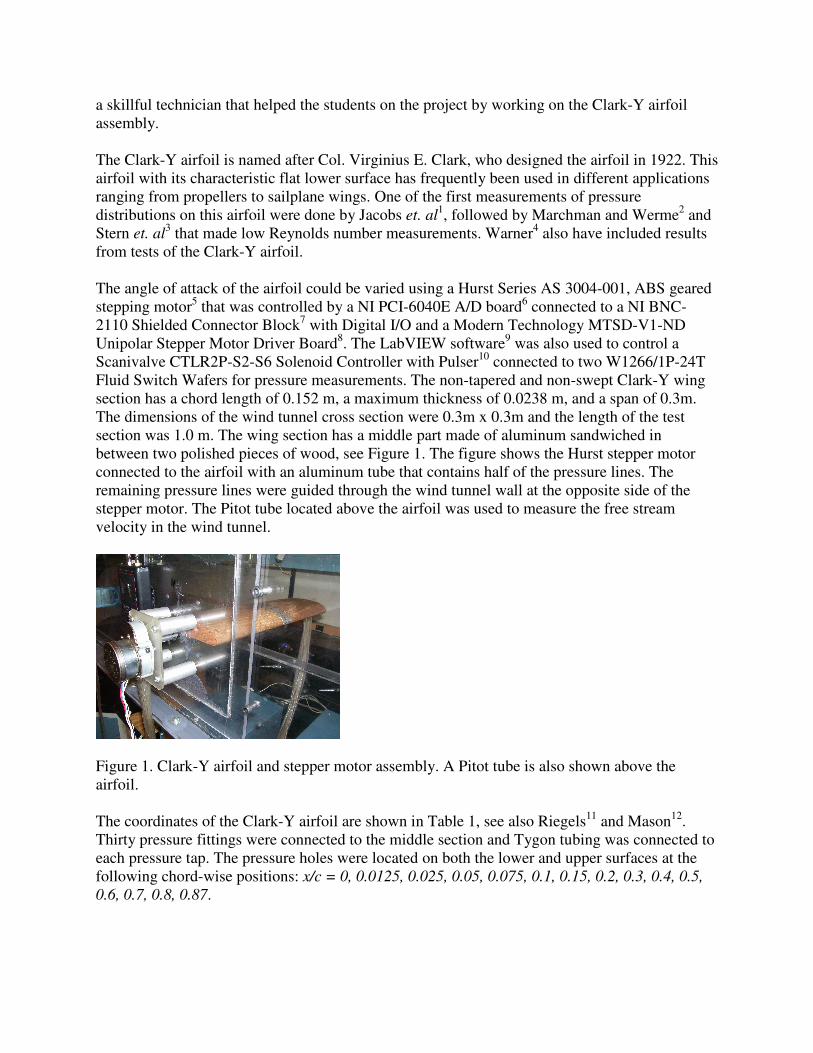
X (mm) Y upper surface (mm) Y lower surface (mm)

0.0 7.1277

1.9 11.0989 3.9304

3.8 13.2372 2.9936

7.6 16.0883 1.8939

11.4 18.0230 1.2830

15.2 19.5504 0.8553

22.8 21.7498 0.3055

30.4 23.1346 0.0611

45.6 23.8270 0.0000

60.8 23.2160 0.0000

76.0 21.4239 0.0000

91.2 18.6339 0.0000

106.4 14.9682 0.0000

121.6 10.6305 0.0000

136.8 5.7022 0.0000

152.0 0.0000 0.0000

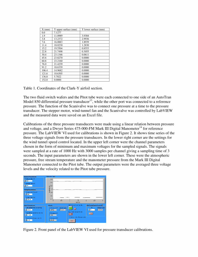
Table 1. Coordinates of the Clark-Y airfoil section. The two fluid switch wafers and the Pitot tube were each connected to one side of an AutoTran Model 850 differential pressure transducer13, while the other port was connected to a reference pressure. The function of the Scanivalve was to connect one pressure at a time to the pressure transducer. The stepper motor, wind-tunnel fan and the Scanivalve was controlled by LabVIEW and the measured data were saved on an Excel file. Calibrations of the three pressure transducers were made using a linear relation between pressure and voltage, and a Dwyer Series 475-000-FM Mark III Digital Manometer14 for reference pressure. The LabVIEW VI used for calibrations is shown in Figure 2. It shows time series of the three voltage signals from the pressure transducers. In the lower right corner are the settings for the wind tunnel speed control located. In the upper left corner were the channel parameters chosen in the form of minimum and maximum voltages for the sampled signals. The signals were sampled at a rate of 1000 Hz with 3000 samples per channel giving a sampling time of 3 seconds. The input parameters are shown in the lower left corner. These were the atmospheric pressure, free stream temperature and the manometer pressure from the Mark III Digital Manometer connected to the Pitot tube. The output parameters were the averaged three voltage levels and the velocity related to the Pitot tube pressure.

Figure 2. Front panel of the LabVIEW VI used for pressure transducer calibrations.

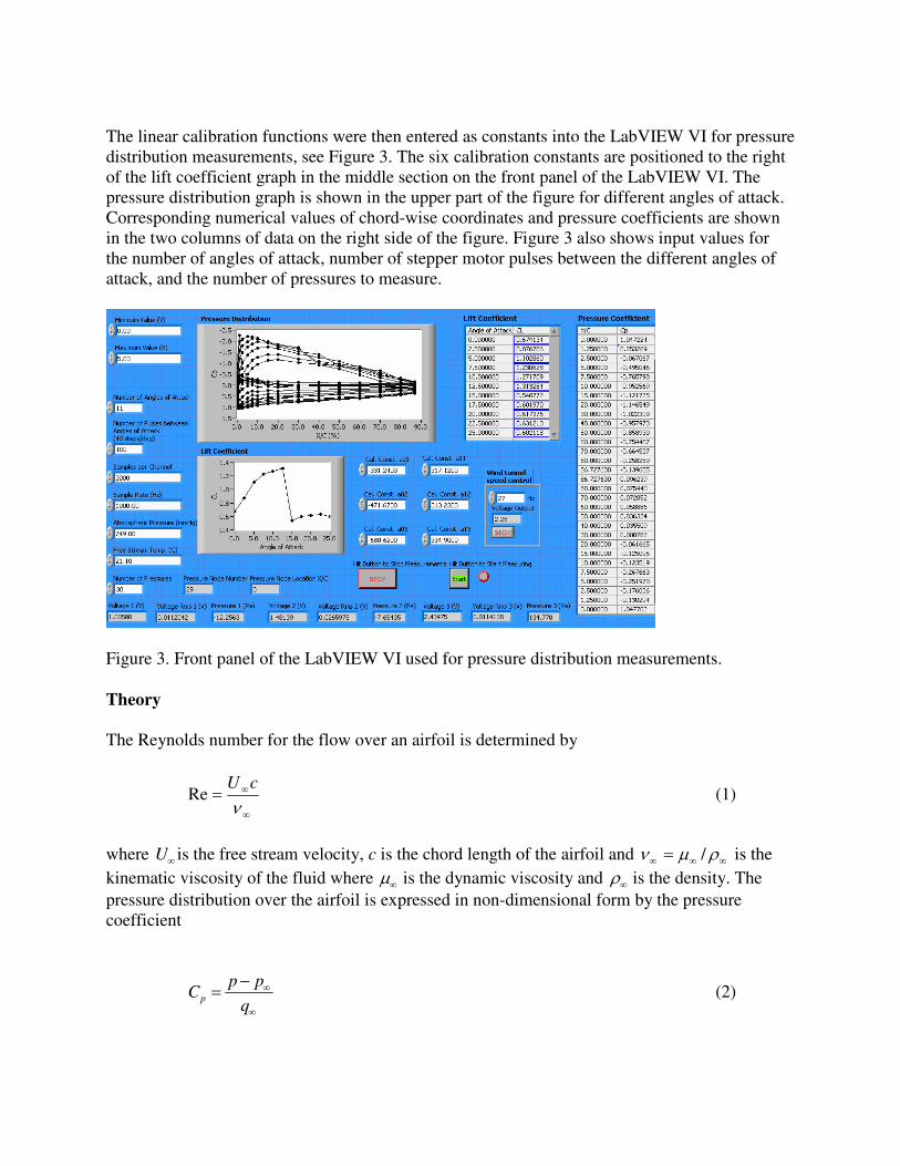
The linear calibration functions were then entered as constants into the LabVIEW VI for pressure distribution measurements, see Figure 3. The six calibration constants are positioned to the right of the lift coefficient graph in the middle section on the front panel of the LabVIEW VI. The pressure distribution graph is shown in the upper part of the figure for different angles of attack. Corresponding numerical values of chord-wise coordinates and pressure coefficients are shown in the two columns of data on the right side of the figure. Figure 3 also shows input values for the number of angles of attack, number of stepper motor pulses between the different angles of attack, and the number of pressures to measure.

Figure 3. Front panel of the LabVIEW VI used for pressure distribution measurements. Theory

The Reynolds number for the flow over an airfoil is determined by

∞

∞=ν

cURe (1)

where U∞ is the free stream velocity, c is the chord length of the airfoil and ∞∞∞ = ρµν / is the

kinematic viscosity of the fluid where µ∞ is the dynamic viscosity and ρ∞ is the density. The

pressure distribution over the airfoil is expressed in non-dimensional form by the pressure coefficient

Cp =p − p∞

q∞

(2)

where p is the surface pressure measured at different locations on the airfoil surface, and p∞ ,

q∞ = ρ∞U∞

2 /2 are the free stream static and dynamic pressure, respectively. The pressure

coefficient can also be related to the velocity distribution U around the airfoil through

Cp =1−U

U∞

2

(3)

The free stream velocity can be determined from Bernoulli equation

po = p∞ +1

2ρ∞U∞

2 (4)

U∞ =2 po − p∞( )

ρ∞

(5)

where po is the stagnation pressure as measured using a Pitot tube. The lift force FL is related to

the dimensionless lift coefficient CL

CL =FL

acq∞

(6)

where a is the spanwise length of the wing section. The drag coefficient CD is determined by the

corresponding equation

CD =FD

acq∞

(7)

where FD is the drag force. The angle of attackα is defined as the angle between the free stream

flow and the straight line between the leading and trailing edges of the airfoil. Under the assumptions of negligible friction, a thin airfoil and a small angle of attack, it is possible to derive the following relation between the lift coefficient and the pressure coefficient

( ) dxCCc

Cc

uplpL ∫ −=0

,,

1 (8)

where Cp,l , Cp,u are the pressure coefficients on the lower and upper surfaces of the airfoil,

respectively. Using this approach, the lift coefficient is simply the enclosed area from the pressure coefficient distribution.

CosmosFloWorks Calculations

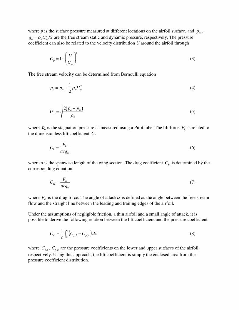
This section shows a portion of a tutorial that was written by the author of this paper for comparisons with experimental results as detailed in the introduction. This tutorial has also been used in the introduction to engineering course to introduce the freshman students to CAD modeling using SolidWorks software and to show students the numerical simulation capabilities of the CosmosFloWorks software package. A model of the airfoil was created in SolidWorks and the part was then exported to CosmosFloWorks. First, the coordinates for the Clark-Y airfoil from Table 1 were imported into SolidWorks in the form of a Clark-Y.sldcrv file. Next, the airfoil profile was extruded to the same spanwise length as the real model in the wind tunnel. A trimetric view of the finished wing section in SolidWorks is shown in Figure 4.

Figure 4. The finished model of the Clark-Y wing section in SolidWorks.

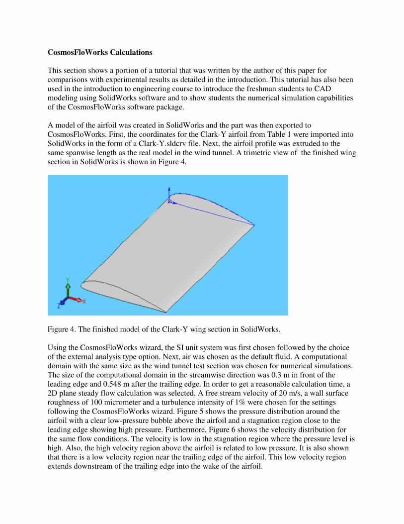
Using the CosmosFloWorks wizard, the SI unit system was first chosen followed by the choice of the external analysis type option. Next, air was chosen as the default fluid. A computational domain with the same size as the wind tunnel test section was chosen for numerical simulations. The size of the computational domain in the streamwise direction was 0.3 m in front of the leading edge and 0.548 m after the trailing edge. In order to get a reasonable calculation time, a 2D plane steady flow calculation was selected. A free stream velocity of 20 m/s, a wall surface roughness of 100 micrometer and a turbulence intensity of 1% were chosen for the settings following the CosmosFloWorks wizard. Figure 5 shows the pressure distribution around the airfoil with a clear low-pressure bubble above the airfoil and a stagnation region close to the leading edge showing high pressure. Furthermore, Figure 6 shows the velocity distribution for the same flow conditions. The velocity is low in the stagnation region where the pressure level is high. Also, the high velocity region above the airfoil is related to low pressure. It is also shown that there is a low velocity region near the trailing edge of the airfoil. This low velocity region extends downstream of the trailing edge into the wake of the airfoil.

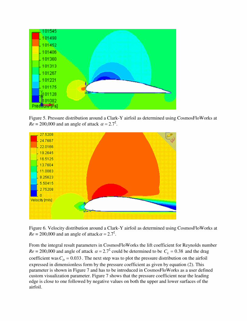
Figure 5. Pressure distribution around a Clark-Y airfoil as determined using CosmosFloWorks at

Re = 200,000 and an angle of attack α = 2.7�.

Figure 6. Velocity distribution around a Clark-Y airfoil as determined using CosmosFloWorks at

Re = 200,000 and an angle of attack α = 2.7�. From the integral result parameters in CosmosFloWorks the lift coefficient for Reynolds number

Re = 200,000 and angle of attack α = 2.7� could be determined to be 38.0=LC and the drag

coefficient was 033.0=DC . The next step was to plot the pressure distribution on the airfoil

expressed in dimensionless form by the pressure coefficient as given by equation (2). This parameter is shown in Figure 7 and has to be introduced in CosmosFloWorks as a user defined custom visualization parameter. Figure 7 shows that the pressure coefficient near the leading edge is close to one followed by negative values on both the upper and lower surfaces of the airfoil.

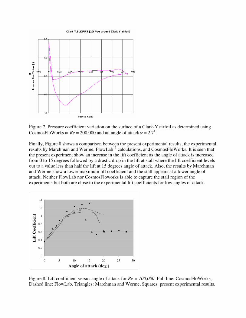
Figure 7. Pressure coefficient variation on the surface of a Clark-Y airfoil as determined using

CosmosFloWorks at Re = 200,000 and an angle of attack α = 2.7�.

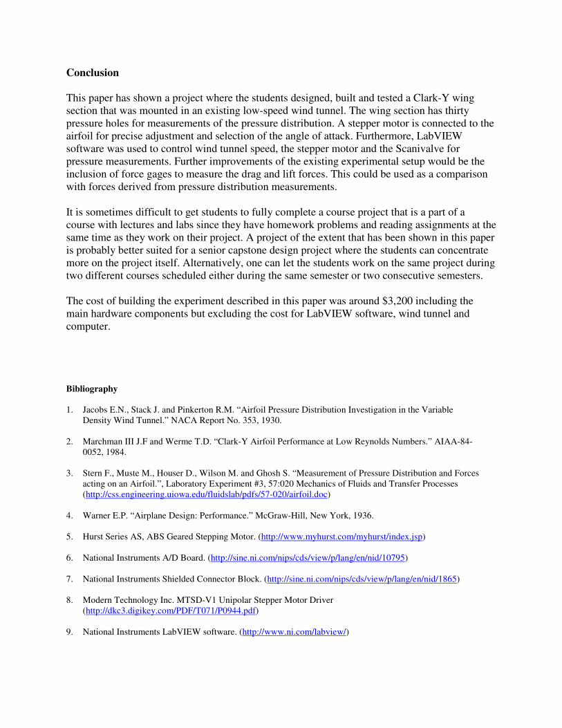
Finally, Figure 8 shows a comparison between the present experimental results, the experimental results by Marchman and Werme, FlowLab15 calculations, and CosmosFloWorks. It is seen that the present experiment show an increase in the lift coefficient as the angle of attack is increased from 0 to 15 degrees followed by a drastic drop in the lift at stall where the lift coefficient levels out to a value less than half the lift at 15 degrees angle of attack. Also, the results by Marchman and Werme show a lower maximum lift coefficient and the stall appears at a lower angle of attack. Neither FlowLab nor CosmosFloworks is able to capture the stall region of the experiments but both are close to the experimental lift coefficients for low angles of attack.

0

0.2

0.4

0.6

0.8

1

1.2

1.4

0 5 10 15 20 25 30

Angle of attack (deg.)

Lif

t C

oef

fici

ent

Figure 8. Lift coefficient versus angle of attack for Re = 100,000. Full line: CosmosFloWorks, Dashed line: FlowLab, Triangles: Marchman and Werme, Squares: present experimental results.

Conclusion

This paper has shown a project where the students designed, built and tested a Clark-Y wing section that was mounted in an existing low-speed wind tunnel. The wing section has thirty pressure holes for measurements of the pressure distribution. A stepper motor is connected to the airfoil for precise adjustment and selection of the angle of attack. Furthermore, LabVIEW software was used to control wind tunnel speed, the stepper motor and the Scanivalve for pressure measurements. Further improvements of the existing experimental setup would be the inclusion of force gages to measure the drag and lift forces. This could be used as a comparison with forces derived from pressure distribution measurements. It is sometimes difficult to get students to fully complete a course project that is a part of a course with lectures and labs since they have homework problems and reading assignments at the same time as they work on their project. A project of the extent that has been shown in this paper is probably better suited for a senior capstone design project where the students can concentrate more on the project itself. Alternatively, one can let the students work on the same project during two different courses scheduled either during the same semester or two consecutive semesters. The cost of building the experiment described in this paper was around $3,200 including the main hardware components but excluding the cost for LabVIEW software, wind tunnel and computer.

Bibliography

1. Jacobs E.N., Stack J. and Pinkerton R.M. “Airfoil Pressure Distribution Investigation in the Variable

Density Wind Tunnel.” NACA Report No. 353, 1930.

2. Marchman III J.F and Werme T.D. “Clark-Y Airfoil Performance at Low Reynolds Numbers.” AIAA-84-0052, 1984.

3. Stern F., Muste M., Houser D., Wilson M. and Ghosh S. “Measurement of Pressure Distribution and Forces

acting on an Airfoil.”, Laboratory Experiment #3, 57:020 Mechanics of Fluids and Transfer Processes (http://css.engineering.uiowa.edu/fluidslab/pdfs/57-020/airfoil.doc)

4. Warner E.P. “Airplane Design: Performance.” McGraw-Hill, New York, 1936.

5. Hurst Series AS, ABS Geared Stepping Motor. (http://www.myhurst.com/myhurst/index.jsp)

6. National Instruments A/D Board. (http://sine.ni.com/nips/cds/view/p/lang/en/nid/10795)

7. National Instruments Shielded Connector Block. (http://sine.ni.com/nips/cds/view/p/lang/en/nid/1865)

8. Modern Technology Inc. MTSD-V1 Unipolar Stepper Motor Driver (http://dkc3.digikey.com/PDF/T071/P0944.pdf)

9. National Instruments LabVIEW software. (http://www.ni.com/labview/)

10. Scanivalve Corp. (http://www.scanivalve.com/) CTLR2/S2-S6 & CTLR2P/S2-S6 Solenoid Controllers Instruction Manual.

11. Riegels F.W. “Airfoil Sections.” Butterworths, London, 1961.

12. Mason W.H. “Experiment 7-Aero/Hydrodynamic Testing.” (http://www.aoe.vt.edu/~devenpor/aoe3054/manual/expt7/text.html)

13. AutoTran Inc. Series 850. (http://www.autotraninc.com/850.html)

14. Dwyer Series 475 Mark III Digital Manometer. (http://www.dwyer-inst.com/htdocs/pdffiles/iom/pressure/475_iom.pdf)

15. Kulkarni A. and Moeykens S. “Flow Over a ClarkY Airfoil.” FlowLab Exercises. (http://flowlab.fluent.com/exercise/ex6.htm)