abstract - school of computing, engineering and · pdf filespider diagrams: a diagrammatic...
TRANSCRIPT

Spider Diagrams: a diagrammatic reasoning system
John Howse, Fernando Molina, John Taylor
School of Computing and Mathematical Sciences
University of Brighton, UK
{John.Howse, F.Molina, John.Taylor}@brighton.ac.uk
Stuart Kent
Computing Laboratory
University of Kent, Canterbury, UK
Abstract
Spider diagrams combine and extend Venn diagrams and Euler circles to express constraints on sets and their
relationships with other sets. These diagrams can be used in conjunction with object-oriented modelling notations such as
the Unified Modelling Language. This paper summarises the main syntax and semantics of spider diagrams. It also
introduces inference rules for reasoning with spider diagrams and a rule for combining spider diagrams. This system is
shown to be sound but not complete. Disjunctive diagrams are considered as one possible way of enriching the system in
order to combine spider diagrams so that no semantic information is lost. Subsystems of spider diagrams which include
disjunctive diagrams are shown to be sound and complete.
Keywords Diagrammatic reasoning, visual formalisms.
1. Introduction
Diagrammatic notations involving circles or closed curves, which we will call contours, have been in use since at least
the Middle Ages [10]. In the middle of the 18th century, the Swiss mathematician Leonhard Euler introduced the notation
we now call Euler circles (or Euler diagrams) [2] for the representation of classical syllogisms. This notation uses the
topological properties of enclosure, exclusion and intersection to represent the set-theoretic notions of subset, disjoint sets,
and intersection, respectively. The 19th century logician John Venn [15] modified this notation to represent logical
propositions. In Venn diagrams all contours must intersect. Moreover, for each non-empty subset of the contours, there

2
must be a connected region of the diagram, such that the contours in this subset intersect at exactly that region. Shading is
then used to show that a particular region represents the empty set.
Venn diagrams are expressive as a visual notation for writing constraints on sets and their relationships with other sets,
but complicated to draw because all possible intersections have to be drawn and then some regions shaded. Drawing the
Venn diagram of four or more sets is quite challenging. More [11], in the late 1950s, developed an algorithm for adding a
new contour to a Venn diagram. It is possible to add contours indefinitely, but the contours quickly assume weird and
wonderful shapes, and the resulting diagram is very complicated and difficult to follow. Indeed, it is rare to see Venn
diagrams of four or more contours. On the other hand, Euler circles are intuitive and easier to draw, but are not as
expressive as Venn diagrams because they lack provisions for shading.
An indication of the popularity and intuitiveness of Venn and Euler diagrams is the fact that they are used in
elementary schools for teaching set theory as an introduction to mathematics. In fact, it is usually a hybrid of the two
notations that is used for teaching purposes; in view of their relative merits, it does seems natural to combine the two
notations, by relaxing the demand that all curves in Venn-diagrams must intersect or by introducing shading into Euler
diagrams. This combined notation forms the basis of spider diagrams.
In the 1890s, Peirce modified Venn diagrams by including X-sequences to introduce elements and disjunctive
information into the system [12]. Recently, full formal semantics and inference rules have been developed for Venn-
Peirce diagrams [14] and Euler diagrams [6]; see also [1, 5] for related work. Shin [14] proves soundness and
completeness results for two systems of Venn-Peirce diagrams.
In object-oriented software development, diagrammatic modelling notations are used to specify systems. Recently, the
Unified Modelling Language (UML) [13] has become the Object Management Group’s (OMG) standard for such
notations. In UML, constraints, such as invariants, preconditions and postconditions, are expressed using the Object
Constraint Language (OCL) [16] essentially a stylised, textual form of first-order predicate logic, which is part of the
UML standard. Constraint diagrams [9, 4] provide a diagrammatic notation for expressing constraints and can be used in
conjunction with UML and OCL.

3
LibrariesCopies
OnHoldcollection
Publications
Reservations
onHoldFor
reserved
publication
Figure 1.1
The constraint diagram in figure 1.1 expresses (amongst other constraints) an invariant on a model of a library system:
for any library object, and any copy of that library which is on hold, that copy's publication must be the same as that
associated with the reservation for which it is on hold. The notation is based on a mixture of Venn and Euler diagrams.
Spider diagrams [3] emerged from work on constraint diagrams. They combine and extend Venn diagrams and Euler
circles to express constraints on sets and their relationships with other sets. This paper summarises the syntax and
semantics of spider diagrams and extends the diagrammatic inference rules for Venn-Peirce diagrams to spider diagrams.
A more detailed discussion of spider diagrams is conducted in section 2, where the main syntax and semantics of the
notation is introduced. Section 3 introduces inference rules for reasoning with spider diagrams and a rule which governs
the equivalence of Venn and Euler forms of spider diagrams, and discusses the rule for combining two spider diagrams.
Section 4 discusses soundness and completeness of the system and indicates one possible way of enriching the system in
order to combine spider diagrams so that no semantic information is lost. Subsystems of spider diagrams which include
disjunctive diagrams are shown to be sound and complete.
2. Spider diagrams
This section introduces the main syntax and semantics of spider diagrams; see [3] for more details and examples.
Spider diagrams are Euler circles augmented with shaded regions and spiders. Spider diagrams also include the concepts
of Schrödinger spiders and projections; these are not necessary for this paper and are omitted from this discussion. In [3],

4
the distinction is made between given and existential spiders; in this paper, all spiders are given (except for the system
introduced in section 4.3).
2.1. Syntactic elements of spider diagrams
A contour is a simple closed plane curve. A boundary contour is not contained in and does not intersect with any other
contour. A district (or basic region) is the bounded area of the plane enclosed by a contour. A region is defined as
follows: any district is a region; if r1 and r2 are regions, then the union, intersection, or difference, of r1 and r2 are regions
provided these are non-empty. A zone (or minimal region) is a region having no other region contained within it. Contours
and regions denote sets.
A spider is a tree with nodes (called feet) placed in different zones; the connecting edges (called legs) are straight
lines. A spider touches a zone if one of its feet appears in that region. A spider may only touch a zone once. A spider is
said to inhabit the region which is the union of the zones it touches. For any spider s, the habitat of s, denoted η(s), is
the region inhabited by s. The set of spiders touching region r is denoted by S(r). Spiders are used to denote elements. In
this paper, all spiders represent given elements. Two distinct spiders denote distinct elements, unless they are joined by a
tie or by a strand.
A tie is a double, straight line (an equals sign) connecting two feet, from different spiders, placed in the same zone. The
nest of spiders s and t, written τ(s, t), is the union of those zones z having the property that the feet of s and t are
connected by a tie in z. Two spiders which have a non-empty nest are referred to as mates. If both the elements denoted
by spiders s and t are in the set denoted by the same zone in the nest of s and t, then s and t denote the same element.
A strand is a wavy line connecting two feet, from different spiders, placed in the same zone. The web of spiders s
and t, written ζ(s, t), is the union of zones z having the property that there is a sequence of spiders
s = s0, s1, s2, … , sn = t
such that, for i = 0, … , n−1, si and si+1 are connected by a tie or by a strand in z. So τ(s, t) is a subregion of ζ(s, t).
Two spiders with a non-empty web are referred to as friends. Two spiders s and t may (but not necessarily must) denote
the same element if that element is in the set denoted by the web of s and t. Clearly, if there is a tie between feet, then a
strand between those feet is redundant. Similarly, multiple strands or ties between the same pairs of feet are redundant.
In later sections, we will need to compare regions across diagrams. To facilitate this, we extend the notation and use,
for example, ζ(s, t, D) and τ(s, t, D) to denote the web and nest respectively of spiders s and t in the diagram D.
5
Every region is a union of zones. A region is shaded if each of its component zones is shaded. A shaded region
containing no spiders denotes the empty set. Shading a region r which includes spiders has the effect of placing an upper
limit on the number of elements in the set denoted by the region. An upper bound is |S(r)|, but this might not be a least
upper bound.
A spider diagram is a finite collection of contours (exactly one of which must be a boundary contour U), spiders,
strands, ties and shaded regions. For any spider diagram D, we use C = C(D), R = R(D), Z = Z(D), Z* = Z*(D) and S
= S(D) to denote the sets of contours, regions, zones, shaded zones and spiders of D, respectively.
The Venn form of a spider diagram contains every possible intersection of contours; otherwise, the diagram is in Euler
form. A spider diagram with n (non-boundary) contours has 2n zones if and only if it is in Venn form.
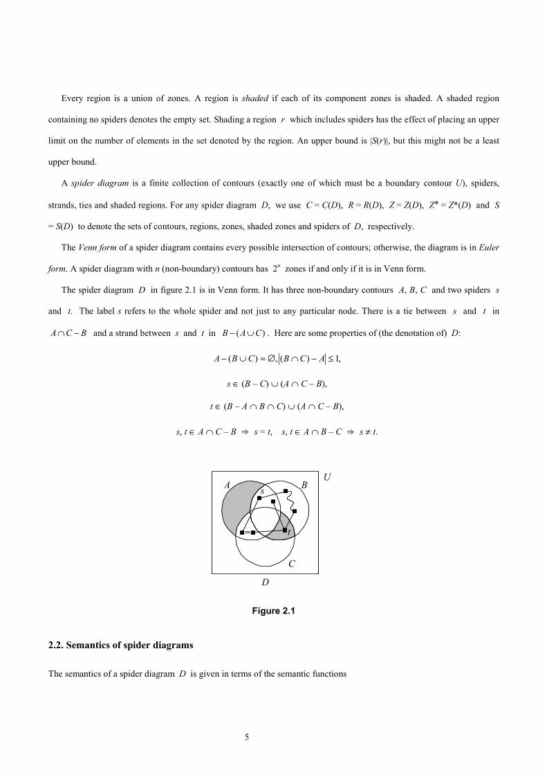
The spider diagram D in figure 2.1 is in Venn form. It has three non-boundary contours A, B, C and two spiders s
and t. The label s refers to the whole spider and not just to any particular node. There is a tie between s and t in
BCA −∩ and a strand between s and t in )( CAB ∪− . Here are some properties of (the denotation of) D:
,1)(,)( ≤−∩∅=∪− ACBCBA
s ∈ (B – C) ∪ (A ∩ C – B),
t ∈ (B – A ∩ B ∩ C) ∪ (A ∩ C – B),
s, t ∈ A ∩ C – B ⇒ s = t, s, t ∈ A ∩ B – C ⇒ s ≠ t.
t
A B
D
C
Us
Figure 2.1
2.2. Semantics of spider diagrams
The semantics of a spider diagram D is given in terms of the semantic functions

6
Ψ : C → Set U, ψ : S → U
where U is a given universal set of D and Set U denotes the power set of U. Contours and regions are interpreted as
subsets of U, and spiders as elements of U. The boundary contour is interpreted as U.
A zone is uniquely defined by the contours containing it and the contours not containing it; its interpretation is the
intersection of the sets denoted by the contours containing it and the complements of the sets denoted by those contours
not containing it. We extend the domain of Ψ to interpret regions as subsets of U. First define Ψ : Z → Set U by
Ψ Ψ Ψ( ) ( ) ( )( ) ( )
z c cc C z c C z
= ∩∈ ∈+ −� �
where C+(z) is the set of contours containing the zone z, C–(z) is the set of contours not containing z and
)()( cc Ψ−=Ψ U , the complement of Ψ(c). Since any region is a union of zones, we may define Ψ : R → Set U by
Ψ Ψ( ) ( )( )
r zz Z r
=∈�
where, for any region r, Z(r) is the set of zones contained in r.
The semantics of a diagram D is the conjunction of the following conditions.
Plane Tiling Condition: All elements fall within sets denoted by zones:
Ψ( )zz Z∈
=� U
Spider Condition: The element denoted by a spider is in the set denoted by the habitat of the spider:
s Ss s
∈∧ ∈ψ η( ) ( ( ))Ψ
Strangers Condition: The elements denoted by two distinct spiders are distinct unless they fall within the set denoted by
the spiders’ web:
)()(,
ts
tsSts
ψψ =∧≠∈
⇒ )),(()(),( tsts ζψψ Ψ∈
Mating Condition: If the elements denoted by two distinct spiders fall within the set denoted by the same zone in the
spiders’ nest, then the elements are equal:
7
)()(),()),((,
ztstsZzSts
Ψ∈∧∧∈∈
ψψτ
⇒ )()( ts ψψ =
Shading Condition: The set denoted by a shaded zone contains no elements other than those denoted by the spiders:
z Z s Sz s
∈ ∈∗∧ ⊆Ψ( ) { ( )}ψ�
We will require the following lemma.
Lemma 2.1. The set denoted by a shaded minimal region not containing the feet of any spiders is empty.
3. Reasoning with spider diagrams
In this section we introduce rules for manipulating single diagrams. Except the last rule, each is an inference rule that
allows us to obtain one diagram from a given diagram by adding or removing diagrammatic elements. The last rule
governs the equivalence of the Euler and Venn forms of spiders diagrams. Throughout this section we use D and D′
respectively to denote the diagrams before and after a single application of one of the rules. To link the semantics of the
‘before’ and ‘after’ diagrams, we assume that UD and UD′ denote the same (universal) set, which we denote U, and that
any two contours or spiders tagged with the same label in D and D′ denote the same set or element.
3.1. Rules of transformation
We introduce seven rules for manipulating single diagrams. The first six are inference rules that allow us to obtain one
diagram from a given diagram by removing, adding or modifying diagrammatic elements. The last rule governs the
equivalence of the Euler and Venn forms of spiders diagrams.
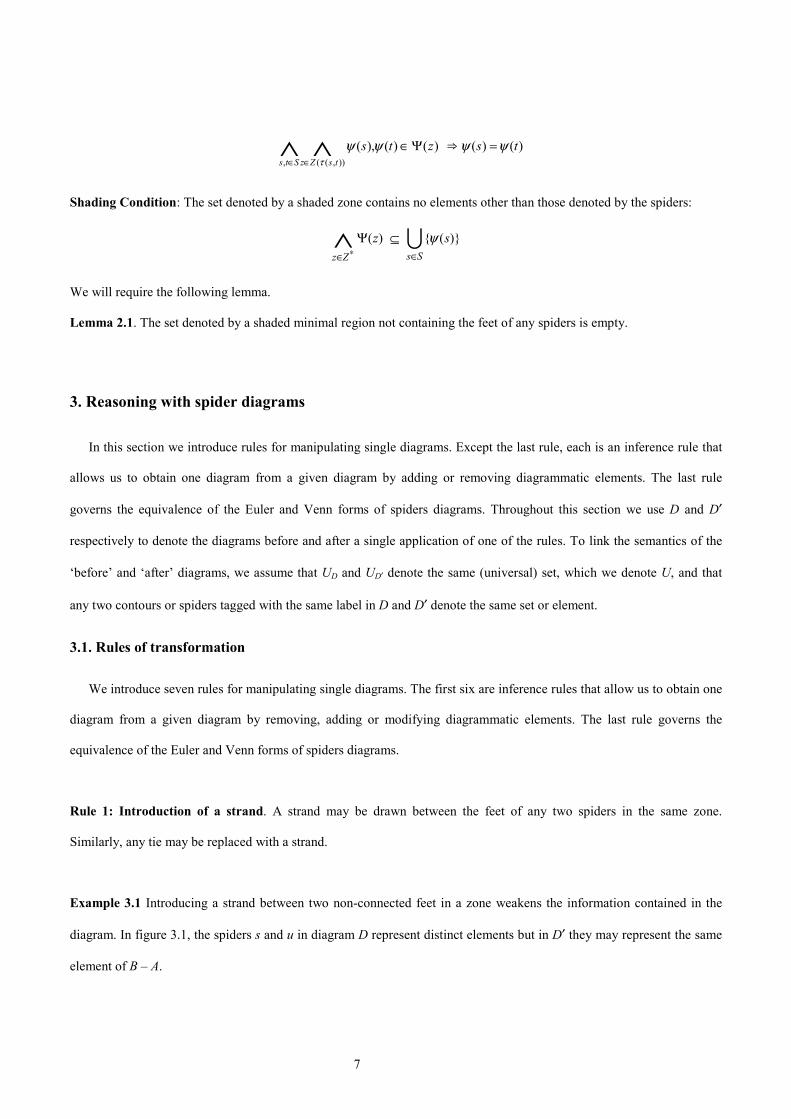
Rule 1: Introduction of a strand. A strand may be drawn between the feet of any two spiders in the same zone.
Similarly, any tie may be replaced with a strand.
Example 3.1 Introducing a strand between two non-connected feet in a zone weakens the information contained in the
diagram. In figure 3.1, the spiders s and u in diagram D represent distinct elements but in D′ they may represent the same
element of B – A.

8
Similarly, replacing a tie between the feet of two spiders with a strand also weakens the semantic information given by
the diagram. If the element denoted by s lies in A – B, then, in D, s and t are necessarily equal whereas in D′ they need not
be.
A B
D
s
D'
A B
s
uut t
U U
Figure 3.1
Rule 2: Spreading the feet of a spider. If a diagram has a spider s, then we may draw a node in any zone z which does
not contain a foot of s and connect it to s. If z contains the foot of another spider t, then we may join the feet of s and t
with a strand or a tie or leave the feet separated in z.
Example 3.2 Rule 3 is illustrated by the diagrams in figure 3.2. The inference from D to D′ requires two applications of
rule 3, but is clearly valid since it just represents a weakening of information. From D we know that the element
corresponding to s belongs to A – B. Having spread its feet in D′, we may only infer that this element belongs to A ∪ B.
In the zone corresponding to A ∩ B, we have chosen to keep the feet of s and t separated; in the zone corresponding to
B – A, we have joined the feet of s and t with a strand.
BA B
s
A
s
D D'
t tU U
Figure 3.2

9
Rule 3: Erasure of a spider. We may erase a complete spider on any non-shaded region and any strand or tie connected
to it. If removing a spider disconnects any component of the ‘strand-tie graph’ in a zone, then the components so formed
should be reconnected using one or more strands to restore the original component.
Example 3.3 In Figure 3.3, erasing the spider u and its two connecting strands disconnects spiders s and t in the zone A –
B. However, the web of s and t is the region A – B, and this should not change with the deletion of u. Hence in D′ the
spiders are explicitly ‘reconnected’ by joining them with a strand.
u
A B
D
sBA
D'
t
s
t
U U
Figure 3.3
Example 3.4 The requirement that the region from which a spider is removed should be non-shaded is a necessary one.
Figure 3.4 illustrates that the removal of a spider from a shaded zone may result in an invalid inference (see section 3.2).
In diagram D, the set corresponding to region A – B contains a single element, whereas in D′, the corresponding set is
empty.
A BA Bs
D D'
U U
Figure 3.4
Rule 4: Erasure of shading. We may erase the shading in an entire zone.
10
A BA B
D D'
U U
s s
Figure 3.5
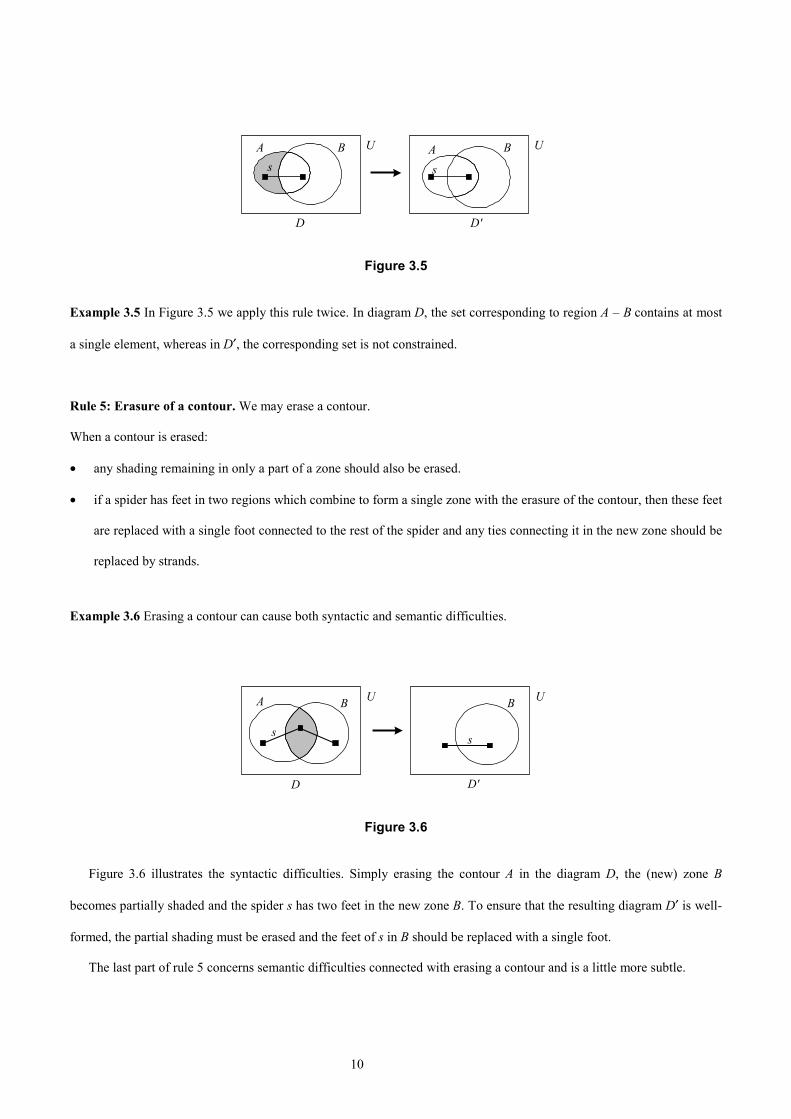
Example 3.5 In Figure 3.5 we apply this rule twice. In diagram D, the set corresponding to region A – B contains at most
a single element, whereas in D′, the corresponding set is not constrained.
Rule 5: Erasure of a contour. We may erase a contour.
When a contour is erased:
• any shading remaining in only a part of a zone should also be erased.
• if a spider has feet in two regions which combine to form a single zone with the erasure of the contour, then these feet
are replaced with a single foot connected to the rest of the spider and any ties connecting it in the new zone should be
replaced by strands.
Example 3.6 Erasing a contour can cause both syntactic and semantic difficulties.
UA B
s
B
s
U
D'D
Figure 3.6
Figure 3.6 illustrates the syntactic difficulties. Simply erasing the contour A in the diagram D, the (new) zone B
becomes partially shaded and the spider s has two feet in the new zone B. To ensure that the resulting diagram D′ is well-
formed, the partial shading must be erased and the feet of s in B should be replaced with a single foot.
The last part of rule 5 concerns semantic difficulties connected with erasing a contour and is a little more subtle.
11
tA B
D
s
A
D'
st
U U
Figure 3.7
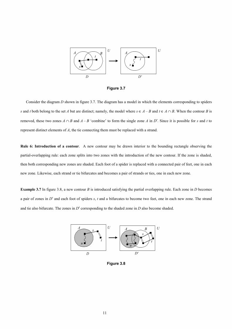
Consider the diagram D shown in figure 3.7. The diagram has a model in which the elements corresponding to spiders
s and t both belong to the set A but are distinct; namely, the model where s ∈ A – B and t ∈ A ∩ B. When the contour B is
removed, these two zones A ∩ B and A – B ‘combine’ to form the single zone A in D′. Since it is possible for s and t to
represent distinct elements of A, the tie connecting them must be replaced with a strand.
Rule 6: Introduction of a contour. A new contour may be drawn interior to the bounding rectangle observing the
partial-overlapping rule: each zone splits into two zones with the introduction of the new contour. If the zone is shaded,
then both corresponding new zones are shaded. Each foot of a spider is replaced with a connected pair of feet, one in each
new zone. Likewise, each strand or tie bifurcates and becomes a pair of strands or ties, one in each new zone.
Example 3.7 In figure 3.8, a new contour B is introduced satisfying the partial overlapping rule. Each zone in D becomes
a pair of zones in D′ and each foot of spiders s, t and u bifurcates to become two feet, one in each new zone. The strand
and tie also bifurcate. The zones in D′ corresponding to the shaded zone in D also become shaded.
A s Bs
A
tu u
t
D D'
U U
Figure 3.8

12
Rule 7: Equivalence of Venn and Euler forms. We may replace a diagram D in which some regions do not exist by a
diagram V(D) in Venn form where those regions are shaded. All other diagrammatic elements—other shaded regions,
spiders, strands and ties—remain unchanged.
Conversely, we may replace a diagram D in Venn form which has a set of shaded zones containing no spider by a
diagram E where (some of) those regions do not exist. Again, all other diagrammatic elements—other shaded regions,
spiders, strands and ties—remain unchanged.
The transition from the Euler to the Venn form of a spider diagram is algorithmic. There are various known algorithms
for constructing a Venn diagram with n contours—for example, see [6]. Given a spider diagram D in Euler form, first
construct the underlying Venn diagram whose set of contours is C(D). Shade any zones which were not present in the
original Euler form D. Finally add spiders, strands and ties in order to replicate the strand-tie graph in each zone of D. The
resulting spider diagram is V(D), the Venn form of D.
A B
C
A B
C
ssU
D'
rr
tt
D
U
Figure 3.9
Example 3.8 Figure 3.9 illustrates the equivalence between the Euler and Venn forms of a spider diagram. The Euler
form D does not contain zones corresponding to A B C∩ ∩ or A B C∩ ∩ . In the Venn form D′, the corresponding
regions are shaded, but the strand-tie graph in every other zone is the same as the corresponding graph in D.
3.2. Comparing regions
Later we will need to be able to identify corresponding regions in different diagrams. For simplicity, we consider the
case where a diagram D′ is obtained from a diagram D by adding contours, so that
C(D) ⊆ C(D′).
There is a natural mapping

13
α: Z(D) → R(D′)
which may be defined inductively, with the inductive step as follows. Suppose that D′ is obtained from D by adding a
single contour. According to Rule 6, each zone z in D bifurcates into two zones zin and zout in D′; zin is that part of z
enclosed within the new contour and zout is that part of z lying outside the new contour (see Figure 3.10). In this case, we
define
α(z) = zin ∪ zout.
Given any zone z′ in D′, there is a unique zone z in D such that z′ ⊆ α(z). The association z′ z defines a mapping
β: Z(D′) → Z(D).
The mappings α and β are illustrated in figure 3.10.
A B
D
A
D'
C
B
zoutz
inz
UU
α(z) = zin ∪ zout, β(zin) = z = β(zout)
Figure 3.10
By taking unions of zones, these mappings extend to mappings
α: R(D) → R(D′), β: R(D′) → R(D).
These mappings are related as follows. For all regions r ∈ R(D), βα(r) = r and for all regions r′ ∈ R(D′), r′ ⊆ αβ(r′). The
first of these statements says that β is a left inverse for α and α is a right inverse for β. It follows that α is injective and β
is surjective. We will need the following lemma.
Lemma 3.1 Let D′ be the diagram formed from D by adding a contour C′ satisfying the partial overlapping rule. If the
zones zin and zout in D′ are formed from the zone z in D as described above, then z is equivalent to the union of the two
zones zin and zout.
14
Ψ(z, D) = Ψ(zin, D′) ∪ Ψ(zout, D′)
3.3. Combining diagrams
Given two diagrams, D1 and D2, we wish to combine them to produce a single diagram D which retains as much of
their combined semantic information as possible. Of course, this is only meaningful if the pair D1, D2 is consistent. In this
section we describe the construction of such a combined diagram D. Even in simple cases, some information contained in
the pair D1, D2 will be lost in the combination. In the next section, we will indicate one possible way of enriching the
system of spider diagrams to overcome this problem.
Suppose two diagrams D1 and D2 are given which do not contain conflicting information. To simplify the process of
combination, we first construct the equivalent Venn form of each diagram, V(D1) and V(D2) respectively. The combined
diagram clearly must contain any contour which appears in either D1 or D2, so the first step in combining the diagrams is
to construct a Venn diagram whose set of contours is
C(D1) ∪ C(D2).
From this underlying Venn diagram, we add diagrammatic elements—shading, spiders, strands and ties—to produce
the final combined diagram D. Since D is obtained from each of the diagrams V(D1) and V(D2) by adding contours, the
‘corresponding region’ mappings introduced in the previous section are defined between V(D1) and D and between V(D2)
and D. These are denoted, respectively, α1, β1 and α2, β2.
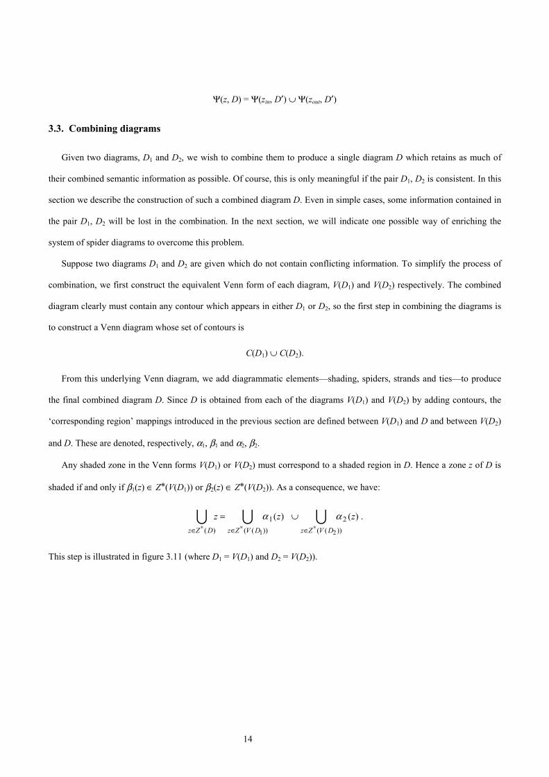
Any shaded zone in the Venn forms V(D1) or V(D2) must correspond to a shaded region in D. Hence a zone z of D is
shaded if and only if β1(z) ∈ Z*(V(D1)) or β2(z) ∈ Z*(V(D2)). As a consequence, we have:
z z zz Z D z Z V D z Z V D∈ ∈ ∈∗ ∗ ∗
= ∪( ) ( ( )) ( ( ))
( ) ( )� � �α α1 2
1 2
.
This step is illustrated in figure 3.11 (where D1 = V(D1) and D2 = V(D2)).
15
A B
D1 D2
A C
A B
CD
UU
U
Figure 3.11
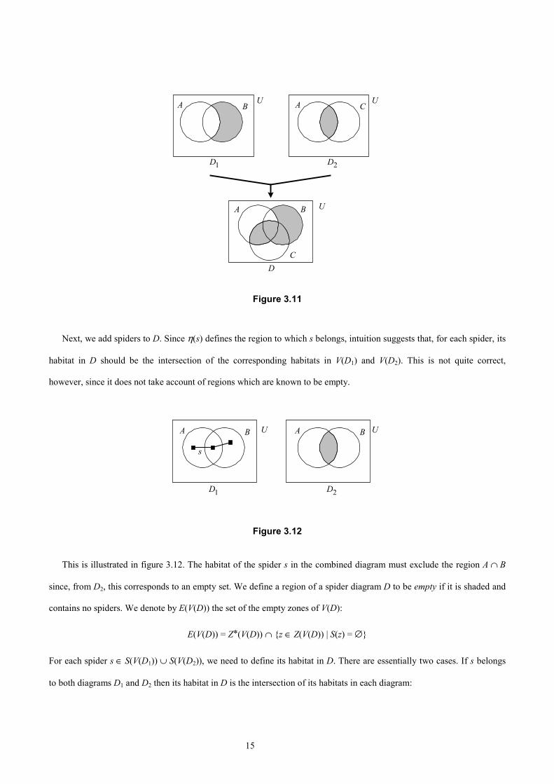
Next, we add spiders to D. Since η(s) defines the region to which s belongs, intuition suggests that, for each spider, its
habitat in D should be the intersection of the corresponding habitats in V(D1) and V(D2). This is not quite correct,
however, since it does not take account of regions which are known to be empty.
D1 D2
A BA B
s
UU
Figure 3.12
This is illustrated in figure 3.12. The habitat of the spider s in the combined diagram must exclude the region A ∩ B
since, from D2, this corresponds to an empty set. We define a region of a spider diagram D to be empty if it is shaded and
contains no spiders. We denote by E(V(D)) the set of the empty zones of V(D):
E(V(D)) = Z*(V(D)) ∩ {z ∈ Z(V(D)) | S(z) = ∅}
For each spider s ∈ S(V(D1)) ∪ S(V(D2)), we need to define its habitat in D. There are essentially two cases. If s belongs
to both diagrams D1 and D2 then its habitat in D is the intersection of its habitats in each diagram:

16
s ∈ S(V(D1)) ∩ S(V(D2)) ⇒ η(s, D) = α1(η(s, (V(D1))) ∩ α2(η(s, V(D2)))
If s belongs to exactly one of the diagrams D1 and D2 then its habitat in D is reduced by removing from it the empty zones
in the other diagram:
s ∈ S(V(D1)) – S(V(D2)) ⇒ η(s, D) = α1(η(s, (V(D1))) – α 22
( )( ( ))
zz E V D∈
��
��� .
With these definitions, the composition of the two diagrams in figure 3.12 is given in figure 3.13.
D
A B
s
U
Figure 3.13
Finally, we consider strands and ties. Suppose two spiders are such that each has a foot in a zone z of the combined
diagram D. Then z corresponds to zones z1 = β1(z) and z2 = β2(z) in V(D1) and V(D2), respectively. Again there are several
cases to consider.
• If neither diagram V(D1) nor V(D2) contains both spiders, then they should be joined by a strand in z. In this case, one
spider belongs to V(D1) and the other belongs to V(D2), so we have no information concerning their equality or
otherwise if they belong to z; hence the spiders should be connected in the most general way.
• If exactly one of the diagrams, V(Di) say, contains both spiders, then they should be connected in z in the same
manner as in zi.
• If both diagrams contain both spiders then:
− they are connected by a tie in z if they are joined by a tie in one of the regions z1, z2 and a tie or strand in the other
region;
− they are not connected in z if they are not connected one of the regions z1, z2 and are either not connected or
connected by a strand in the other region;
17
− otherwise they are connected by a strand in z.
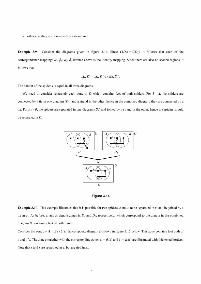
Example 3.9. Consider the diagrams given in figure 3.14. Since C(D1) = C(D2), it follows that each of the
correspondence mappings α1, β1, α2, β2 defined above is the identity mapping. Since there are also no shaded regions, it
follows that
η(t, D) = η(t, D1) ∩ η(t, D2).
The habitat of the spider s is equal in all three diagrams.
We need to consider separately each zone in D which contains feet of both spiders. For B – A, the spiders are
connected by a tie in one diagram (D2) and a strand in the other; hence in the combined diagram, they are connected by a
tie. For A ∩ B, the spiders are separated in one diagram (D1) and joined by a strand in the other; hence the spiders should
be separated in D.
A B
t
s
D
D2D1
A B
t
sA B
t
sU
U
U
Figure 3.14
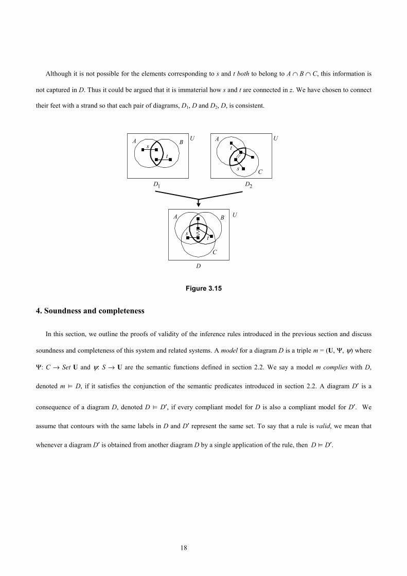
Example 3.10. This example illustrates that it is possible for two spiders, s and t, to be separated in z1 and be joined by a
tie in z2. As before, z1 and z2 denote zones in D1 and D2, respectively, which correspond to the zone z in the combined
diagram D containing feet of both s and t.
Consider the zone z = A ∩ B ∩ C in the composite diagram D shown in figure 3.15 below. This zone contains feet both of
s and of t. The zone z together with the corresponding zones z1 = β1(z) and z2 = β2(z) are illustrated with thickened borders.
Note that s and t are separated in z1 but are tied in z2.
18
Although it is not possible for the elements corresponding to s and t both to belong to A ∩ B ∩ C, this information is
not captured in D. Thus it could be argued that it is immaterial how s and t are connected in z. We have chosen to connect
their feet with a strand so that each pair of diagrams, D1, D and D2, D, is consistent.
D2
A
C
t
s
D1
A B
ts
A B
ts
C
D
U U
U
Figure 3.15
4. Soundness and completeness
In this section, we outline the proofs of validity of the inference rules introduced in the previous section and discuss
soundness and completeness of this system and related systems. A model for a diagram D is a triple m = (U, Ψ, ψ) where
Ψ: C → Set U and ψ: S → U are the semantic functions defined in section 2.2. We say a model m complies with D,
denoted m ⊨ D, if it satisfies the conjunction of the semantic predicates introduced in section 2.2. A diagram D′ is a
consequence of a diagram D, denoted D ⊨ D′, if every compliant model for D is also a compliant model for D′. We
assume that contours with the same labels in D and D′ represent the same set. To say that a rule is valid, we mean that
whenever a diagram D′ is obtained from another diagram D by a single application of the rule, then D ⊨ D′.
19
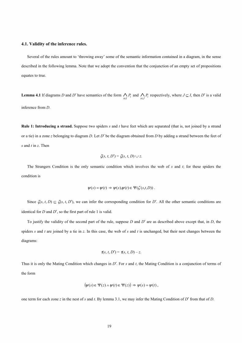
4.1. Validity of the inference rules.
Several of the rules amount to ‘throwing away’ some of the semantic information contained in a diagram, in the sense
described in the following lemma. Note that we adopt the convention that the conjunction of an empty set of propositions
equates to true.
Lemma 4.1 If diagrams D and D′ have semantics of the form ∧∈i I iP and ∧
∈i J iP respectively, where J ⊆ I, then D′ is a valid
inference from D.
Rule 1: Introducing a strand. Suppose two spiders s and t have feet which are separated (that is, not joined by a strand
or a tie) in a zone z belonging to diagram D. Let D′ be the diagram obtained from D by adding a strand between the feet of
s and t in z. Then
ζ(s, t, D′) = ζ(s, t, D) ∪ z.
The Strangers Condition is the only semantic condition which involves the web of s and t; for these spiders the
condition is
)()( ts ψψ = ⇒ )),,(()(),( Dtsts ζψψ Ψ∈ .
Since ζ(s, t, D) ⊆ ζ(s, t, D′), we can infer the corresponding condition for D′. All the other semantic conditions are
identical for D and D′, so the first part of rule 1 is valid.
To justify the validity of the second part of the rule, suppose D and D′ are as described above except that, in D, the
spiders s and t are joined by a tie in z. In this case, the web of s and t is unchanged, but their nest changes between the
diagrams:
τ(s, t, D′) = τ(s, t, D) – z.
Thus it is only the Mating Condition which changes in D′. For s and t, the Mating Condition is a conjunction of terms of
the form
( ))()()()( ztzs Ψ∈∧Ψ∈ ψψ ⇒ )()( ts ψψ = ,
one term for each zone z in the nest of s and t. By lemma 3.1, we may infer the Mating Condition of D′ from that of D.

20
Rule 2: Spreading the feet of a spider. Suppose D′ is obtained from D by spreading the feet of spider s into the zone z.
We consider the semantic conditions that are changed in passing from D to D′.
Spider Condition. Spreading the feet of s extends its habitat so that
η(s, D′) = η(s, D) ∪ z.
Since η(s, D) ⊆ η(s, D′), the spider condition for D′ follows from that for D.
To complete the proof, we suppose z contains a spider t and consider the three cases given in rule 2.
(a) If s and t are joined by a strand in z then ζ(s, t, D′) = ζ(s, t, D) ∪ z so ζ(s, t, D) ⊆ ζ(s, t, D′). Hence the Strangers
Condition for D′ follows from that for D. In this case the Mating Condition is unchanged.
(b) If s and t remain separated in m then their web and nest are unchanged and hence so are the Strangers and Mating
Conditions.
(c) If s and t are joined by a tie in z then ζ(s, t, D′) = ζ(s, t, D) ∪ z and τ(s, t, D′) = τ(s, t, D) ∪ z. The Strangers
Condition for D′ follows as in case (a). To obtain the Mating Condition for D′, we add the conjunct
ψ(s), ψ(t) ∈ Ψ(z) ⇒ ψ(s) = ψ(t)
to the Mating Condition for D. However, from the Spider Condition for D, we know ψ(s) ∉ Ψ(z) since z does not
form part of the habitat of s in D. Therefore the additional conjunct is true and the Mating Condition for D′
follows.
Rule 3: Erasure of shading. Erasing the shading in a zone only changes the Shading Condition by removing conjuncts,
so the validity of the first part of rule 2 follows by lemma 4.1.
Rule 4: Erasure of a spider. The validity of the rule for erasing a spider follows similarly. However, in passing from the
semantics of D to that of D′, one or more conjuncts may be lost from the Spider, Strangers and Mating conditions.
21
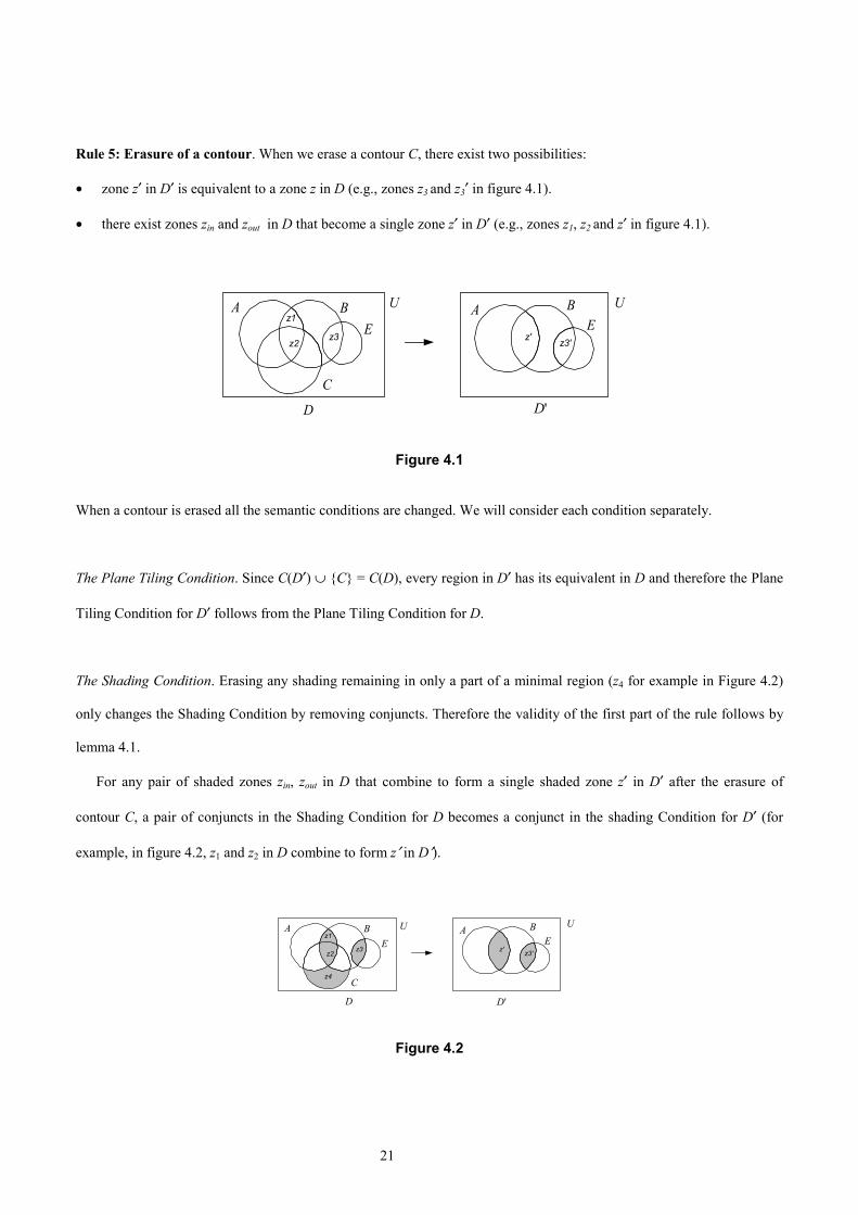
Rule 5: Erasure of a contour. When we erase a contour C, there exist two possibilities:
• zone z′ in D′ is equivalent to a zone z in D (e.g., zones z3 and z3′ in figure 4.1).
• there exist zones zin and zout in D that become a single zone z′ in D′ (e.g., zones z1, z2 and z′ in figure 4.1).
D
A B
'D
A B
C
z1
z'z2
EEz3 z3'
U U
Figure 4.1
When a contour is erased all the semantic conditions are changed. We will consider each condition separately.
The Plane Tiling Condition. Since C(D′) ∪ {C} = C(D), every region in D′ has its equivalent in D and therefore the Plane
Tiling Condition for D′ follows from the Plane Tiling Condition for D.
The Shading Condition. Erasing any shading remaining in only a part of a minimal region (z4 for example in Figure 4.2)
only changes the Shading Condition by removing conjuncts. Therefore the validity of the first part of the rule follows by
lemma 4.1.
For any pair of shaded zones zin, zout in D that combine to form a single shaded zone z′ in D′ after the erasure of
contour C, a pair of conjuncts in the Shading Condition for D becomes a conjunct in the shading Condition for D′ (for
example, in figure 4.2, z1 and z2 in D combine to form z′ in D′).
A B
'D
A B
C
D
z1
z'z2
z4
EEz3 z3'
U U
Figure 4.2

22
By the Shading Condition for D we have
�Ss
in sz∈
⊆Ψ )}({)( ψ and �Ss
out sz∈
⊆Ψ )}({)( ψ
whence
�Ss
outin szz∈
⊆Ψ∪Ψ )}({))()(( ψ
which is equivalent, by lemma 3.1, to
�Ss
sz∈
⊆′Ψ )}({)( ψ
the Shading Condition for z′ in D′.
The third and final possibility is that a shaded minimal region z in D (e.g., z3 in figure 4.2) is equivalent to a unique
minimal region z′ in D′. Its conjunct in the Shading Condition for D has an equivalent for the shaded minimal region z′ in
the Shading Condition for D′.
Spider Condition. For any spider s, the set denoted by its habitat in D is a subset of the set denoted by its habitat in D′:
η(s, D) ⊆ η(s, D′)
Therefore, we may infer the Spider Condition for D′ from that of D.
Mating Condition. For any tie replaced by a strand connecting spiders r and s in a zone z the Mating Condition changes
by removing the conjunct
)()(),( zsr Ψ∈ψψ ⇒ )()( sr ψψ =
For any other tie connecting spiders r and s in zone z and not having to be replaced by a strand, there exists no region k
containing feet of r or s such that Ψ(z) ∪ Ψ(k) = Ψ′(z′) for some z′ in D′ (otherwise, the tie should be replaced by a
strand) or there exists an equivalent region n′ in D′. Therefore, their nest changes between the diagrams:
τ(s, t, D) ⊆ τ(s, t, D′)

23
and for any conjunct including spiders r and s in the Mating Condition for D, there is a corresponding conjunct in the
Mating Condition for D′.
Strangers Condition. By lemma 3.1, it follows that ζ(r, s, D) ⊆ ζ(r, s, D′)
Therefore for any two spiders r and s in a zone z in D )()( sr ψψ = ⇒ )),(()(),( tssr ζψψ Ψ∈
The Strangers Condition in D′ follows )()( sr ψψ = ⇒ )),((')(),( tssr ζψψ Ψ∈
Rule 6: Introduction of a contour. To identify and keep track of the zones in D′ that arise from ‘splitting’ zones in D
with the introduction of a contour C′. We denote by zin and zout the two zones in D′ which are formed by splitting a zone z
in D; zin is that part of z enclosed within the new contour C′ and zout is that part of z lying outside C′ (see figure 4.3).
A B
D
A
D'
C'
B
zoutz
inz
U U
Figure 4.3
In passing from D to D′ by adding contour C′ as described in the rule, a number of the semantic conditions change. We
consider each condition in turn.
Plane Tiling Condition. The minimal regions in D′ may be grouped in pairs of the form zin, zout for some zone z in D.
Hence the Plane Tiling Condition for D′ follows from the corresponding condition for D by lemma 3.1.
Spider Condition. Suppose a spider s has a foot in the zone z of D. In D′ the foot bifurcates giving a foot in each of the
zones zin and zout in D′. Hence, by lemma 3.1,
Ψ(η(s, D)) = Ψ(η(s, D′)),
24
so the Spider condition for D′ follows from that of D.
Mating Condition. Each tie connecting spiders s and t bifurcates in D′, so lemma 3.1 ensures that the nest of s and t is
unchanged:
τ(s, t, D) = τ(s, t, D′).
Suppose that spiders s and t are joined by a tie in a zone z in D. The Mating Condition for z in D gives
ψ(s), ψ(t) ∈ Ψ(z) ⇒ ψ(s) = ψ(t).
If ψ(s), ψ(t) ∈ Ψ′(zin) ⊆ Ψ(z) then ψ(s) = ψ(t); similarly, if ψ(s), ψ(t) ∈ Ψ′(zout) ⊆ Ψ(z) then ψ(s) = ψ(t). The Mating
Condition for D′ follows.
Strangers Condition. This is similar to the spiders condition. Bifurcating each tie, strand and node of spiders s and t we
ensure that sets denoted by their webs in D and D′ are identical
ζ(s, t, D) = ζ(s, t, D′).
The Strangers Conditions for s and t in D′ then follows from the corresponding condition for D.
Shading Condition. Suppose that z is a zone in D. Then both the zones zin and zout in D′ are also shaded. The Shading
Condition for z, is the following.
�Ss
sz∈
⊆Ψ )}({)( ψ
Since Ψ(z) = Ψ′(zin) ∪ Ψ′(zout), this gives �Ss
in sz∈
⊆Ψ )}({)( ψ and �Ss
out sz∈
⊆Ψ )}({)( ψ
These are precisely the Shading Conditions for zin and zout in D′.

25
Rule 7: Equivalence of Venn and Euler forms.
Given that the transition between the Venn and the Euler form of a spider diagram only affects the representation of
empty minimal regions it is only the Plane Tiling Condition and the Shading Condition which change. Suppose a diagram
D in Venn form has a set ZE*(D) of shaded zones that are not contained in the Euler form D′. The Shading Condition for
D may be separated into terms whose zones belong to Z*(D) – ZE*(D) and terms whose zones belong to ZE*(D):
�SsDZEDZz
sz∈−∈
⊆Ψ∧∗
)}({)()()( *
ψ and �SsDZEz
sz∈∈
⊆Ψ∧ )}({)()(*
ψ
Note that, since Z*(D) – ZE*(D) = Z*(D′), the first collection of conjuncts,
�SsDZEDZz
sz∈−∈
⊆Ψ∧∗
)}({)()()( *
ψ
is equivalent to the Shading Condition for D′.
It can also be shown that the second collection of conjuncts,
�SsDZEz
sz∈∈
⊆Ψ∧ )}({)()(*
ψ
is equivalent to the Plane Tiling Condition for D′
U=Ψ′∈
�)(
)(DZz
z
since any empty zone in ZE*(D) does not exist in D′ and therefore it is not included in the Plane Tiling Condition for D.
Note that the Plane Tiling Condition for the diagram D in Venn form is true since D contains all possible regions.
Combining diagrams
Suppose two diagrams D1 and D2 are given which do not contain conflicting information. Their combined diagram is
formed by adding syntactic elements into the Venn diagram whose set of contours is C(D1) ∪ C(D2). By the rule of
equivalence of Venn and Euler forms and the rule of introducing contours, we may assume, without loss of generality,
that D1 and D2 are in Venn form and have the same sets of contours. Thus C(D) = C(D1) = C(D2). In this case, D1 =
26
V(D1), D2 = V(D2) and the ‘corresponding region’ mappings, α1, β1 and α2, β2, are identity mappings. We consider each of
the semantic conditions for D in turn.
Plane Tiling Condition. Since D is in Venn form, all possible zones appear in the diagram and the Plane Tiling
Condition for D follows.
Spider Condition. Let s be a spider in D. There are two cases to consider.
Suppose that s belongs to both D1 and D2. Then its habitat in D is the intersection of its habitats in D1 and D2: η(s, D)
= η(s, D1) ∩ η(s, D2). In this case we have:
ψ(s) ∈ Ψ(η(s, D1)) ∧ ψ(s) ∈ Ψ(η(s, D2)) (from the Spider Conditions in D1 and D2)
⇒ ψ(s) ∈ Ψ(η(s, D1)) ∩ Ψ(η(s, D2))
⇒ ψ(s) ∈ Ψ(η(s, D1) ∩ =η(s, D2)) (since equivalent regions denote the same set)
⇒ ψ(s) ∈ Ψ(η(s, D))
Suppose that s belongs exactly one of the diagrams; say, s belongs to both D1 but not D2. Then its habitat in D is
η(s, D) = η(s, D1) – �)( 2DEzz
∈.
Now ψ(s) ∈ Ψ(η(s, D1)) from the Spider Condition in D1 and ψ(s) ∉ �)( 2
)(DEz
z∈
Ψ since Ψ(z) = ∅ for any zone z ∈
E(D2), by lemma 2.1. Hence ψ(s) ∈ Ψ(η(s, D)).
Therefore the Spider Condition is satisfied in D.
Strangers Condition. The rule for combining diagrams implies that, for all spiders s, t in D, ζ(s, t, D1) ∩ ζ(s, t, D2) ⊆
ζ(s, t, D). Hence the Strangers Condition for D follows from the Strangers Conditions for D1 and D2.

27
Mating Condition. Let z be a zone in D which forms part of the nest of spiders s and t; that is, z ⊆ τ(s, t, D). Then z
forms part of the nest of s and t in at least one of the diagrams D1 and D2. Therefore the Mating Condition for D follows
from the Mating Conditions for D1 and D2.
Shading Condition. Let z be a shaded zone of D. Then z is shaded in at least one of the diagrams D1 and D2. Suppose
the spider s has a foot in z in the combined diagram D; that is, z ⊆ η(s, D). Then in at least one of the diagrams D1 and D2,
s has a foot in z and z is shaded; that is, z ⊆ η(s, Di) ∩ {z∗ : z∗ ∈ Z∗(Di)} for i = 1 or 2. Hence if x ∈ Ψ(z) then x = ψ(s) for
some s ∈ S(Di) for i = 1 or 2, by the Shading Condition for Di. Since S(D) = S(D1) ∪ S(D2), the Shading Condition for D
follows from the Shading Conditions for D1 and D2.
Hence the rule of combining diagrams is valid.
4.2. Soundness and completeness
We write D ⊢ D′ to denote that the diagram D′ can be obtained from the diagram D by applying a finite sequence
of transformations. Similarly, we write {D1, D2, …, Dn} ⊢ D′ if D′ can be obtained from the set of diagrams {D1, D2,
…, Dn} by applying a finite sequence of transformations, including the rule for (pairwise) combination of diagrams.
The semantics of a set of diagrams is the conjunction of the semantics of the individual diagrams; the boundary
rectangles of all diagrams are interpreted as the same set U and contours with the same labels in different individual
diagrams are interpreted as the same set.
The following soundness rule for the spider diagram system follows by induction from the validity of each of the
transformation rules and the rule for combining diagrams.
Theorem 4.1 If {D1, D2, …, Dn} ⊢ D′ then {D1, D2, …, Dn} ⊨ D′.
However the system of spider diagrams introduced here is not complete, as the following example shows.
28
Example 4.1. In figure 4.4, diagram D′ can be inferred from diagram D, D ⊨ D′. However, when removing spider s
from D, rule 2 would require a strand between spiders t and u in the resulting diagram, a weaker result. The rules of
inference do not allow D′ to be obtained syntactically from D.
tr
A B
s
U
D'
tr
A B
D
U
Figure 4.4
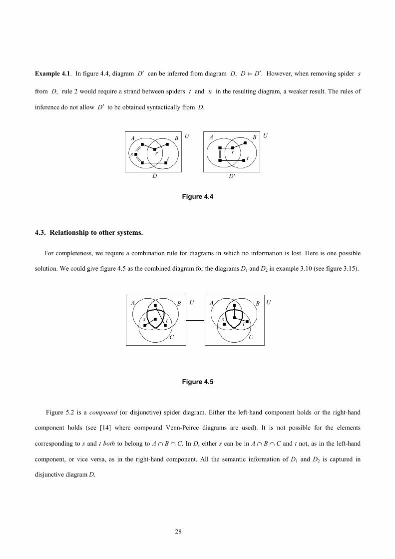
4.3. Relationship to other systems.
For completeness, we require a combination rule for diagrams in which no information is lost. Here is one possible
solution. We could give figure 4.5 as the combined diagram for the diagrams D1 and D2 in example 3.10 (see figure 3.15).
UA B
ts
C
A B
ts
C
U
Figure 4.5
Figure 5.2 is a compound (or disjunctive) spider diagram. Either the left-hand component holds or the right-hand
component holds (see [14] where compound Venn-Peirce diagrams are used). It is not possible for the elements
corresponding to s and t both to belong to A ∩ B ∩ C. In D, either s can be in A ∩ B ∩ C and t not, as in the left-hand
component, or vice versa, as in the right-hand component. All the semantic information of D1 and D2 is captured in
disjunctive diagram D.

29
The semantics of a compound diagram is the disjunction of the semantics of its component unitary diagrams; the
boundary rectangles of the component unitary diagrams are interpreted as the same set U. Contours with the same labels
in different component unitary diagrams of a compound diagram D are interpreted as the same set.
The compound diagram in Figure 4.6 asserts that:
),(),( CBAyBxyxCByCAxyx ∪−∈∧∈•∃∨−∈∧∩∈•∃ .
UA B
C
A B
C
U
D1 D2
Figure 4.6
The diagram in figure 4.6 is part of a subsystem of spider diagrams that is considered in [7]. The system is based on
Venn diagrams and includes compound diagrams. The spiders in this system denote the existence of elements in the
corresponding sets (see [3] for details). The system does not contain strands or ties. We can adapt the rules given earlier
so that they pertain to this system and add in extra rules concerned with compound diagrams to produce a diagrammatic
reasoning system that we can prove to be complete. The basic strategy to prove completeness, i.e., if {D1, D2, …, Dn} ⊨
D′ then {D1, D2, …, Dn} ⊢ D′, is to obtain the diagram that results from combining the individual diagrams in {D1, D2,
…, Dn} and then expanding this combined diagram and D′ in a way similar to disjunctive normal form in symbolic logic.
This proof strategy should extend to most spider/constraint diagram systems. The details of this strategy can be found in
[8].
5. Conclusions
In this paper, we have given the main syntax and semantics of spider diagrams. We have given inference rules, a rule
governing the equivalence of the Venn and Euler forms of spider diagrams and a rule for combining spider diagrams.
These rules have been shown to be sound; but, in some cases, the rules do not give as strong an inference as possible and

30
so the system is not complete. However, we have shown that for a subsystem of spider diagrams that includes compound
diagrams we can prove completeness. Moreover, the strategy for proving completeness should extend to most
spider/constraint diagram systems.
Acknowledgements
We gratefully acknowledge Richard Bosworth, Paul Courtney, Yossi Gil, Richard Mitchell, Dan Simpson and Kees
van Deempter for comments on earlier versions of this paper. Authors Howse and Kent acknowledge support of the UK
EPSRC grant number GR/M02606.
References
1 Allwein, G, Barwise, J (1996) Logical Reasoning with Diagrams, OUP.
2 Euler, L (1772) Lettres a Une Princesse d’Allemagne. Vol. 2, Sur divers subject de physique et de philosophie,
Letters No. 102-108. Basel, Birkhauser.
3 Gil, Y., Howse, J., Kent, S. (1999) Formalizing Spider Diagrams, Proceedings of IEEE Symposium on Visual
Languages (VL99), IEEE Computer Society Press.
4 Gil, Y., Howse, J., Kent, S. (1999) Constraint Diagrams: a step beyond UML, Proceedings of TOOLS USA 1999,
IEEE Computer Society Press.
5 Glasgow, J, Narayanan, N, Chandrasekaran, B (1995) Diagrammatic Reasoning, MIT Press.
6 Hammer, E.M. (1995) Logic and Visual Information, CSLI Publications.
7 Howse, J., Molina, F., Taylor, J., (2000) SD1: A Sound and Complete Diagrammatic Reasoning System, Technical
Report UBITR-2000/3 University of Brighton. (Submitted to LICS2000.)
8 Howse, J., Molina, F., Taylor, J., (2000) SD2: A Sound and Complete Diagrammatic Reasoning System, Technical
Report UBITR-2000/4 University of Brighton. (Submitted to VL2000.)
9 Kent, S. (1997) Constraint Diagrams: Visualising Invariants in Object Oriented Models. Proceedings of OOPSLA 97
10 Lull, R. (1517) Ars Magma. Lyons.

31
11 More, T. (1959) On the construction of Venn diagrams. Journal of Symbolic Logic, 24.
12 Peirce, C (1933) Collected Papers. Vol. 4. Harvard University Press.
13 Rumbaugh, J., Jacobson, I., Booch, G. (1999) Unified Modeling Language Reference Manual. Addison-Wesley.
14 Shin, S-J (1994) The Logical Status of Diagrams. CUP.
15 Venn, J (1880) On the Diagrammatic and Mechanical Representation of Propositions and Reasonings, Phil. Mag.
123.
16 Warmer, J. and Kleppe, A. (1998) The Object Constraint Language: Precise Modeling with UML, Addison-Wesley.