ABSTRACT

Title of Thesis: OBSERVER-BASED FEEDBACKCONTROL FOR STABILIZATIONOF COLLECTIVE MOTION

Seth Ochse Napora, Master of Science, 2011

Thesis directed by: Professor Derek A. PaleyDepartment of Aerospace Engineering

Multi-vehicle control has applications in weather monitoring and ocean sam-

pling. Previous work in this field has produced theoretically justified algorithms for

stabilization of parallel and circular motions of self-propelled Newtonian particles

using measurements of relative position and relative velocity. This paper describes

an observer-based feedback control algorithm for stabilization of parallel and cir-

cular motions using measurements of relative position only. The algorithm utilizes

information about vehicle dynamics and turning rates to estimate relative velocity.

Theoretical justification is provided for the vehicle model, and numerical simulations

suggest that the algorithm extends to a three-dimensional rigid body model. The

algorithm has been implemented on a laboratory-scale underwater vehicle testbed,

and we describe the results of experimental validation in the University of Mary-

land’s Neutral Buoyancy Research Facility.

OBSERVER-BASED FEEDBACK CONTROL FORSTABILIZATION OF COLLECTIVE MOTION

by

Seth Ochse Napora

Thesis submitted to the Faculty of the Graduate School of theUniversity of Maryland, College Park in partial fulfillment

of the requirements for the degree ofMaster of Science

2011

Advisory Committee:Professor Derek A. Paley, ChairProfessor Robert M. SannerProfessor David Akin

c© Copyright bySeth Ochse Napora

2011

Dedication

I would like to dedicate this work to my brother and parents. They have

always been there and provided me with help and support.

ii

Acknowledgments

I would like to take this opportunity to thank everyone that has helped me

throughout my academic career. During my studies at the University of Maryland,

I have thoroughly enjoyed working in the Collective Dynamics and Control Labo-

ratory focusing on the design, development, and implementation of an autonomous

underwater vehicle testbed. This research would not have been possible without the

assistance of Dr. Derek A. Paley, my mentor. His thorough advice and insightful

suggestions have proven to be invaluable to my research. Additionally, I would also

like to specifically recognize Levi DeVries and Nitin Sydney. Their consistent in-

volvement in the submarine testing over the years has helped produce informative

and useful results which have been noted throughout this paper. Also, Rochelle

Mellish, Cammy Peterson, and Sachit Butail have been helpful in providing theo-

retical input. Finally, I am grateful to the members of the Collective Dynamics and

Control Laboratory and the Space Systems Laboratory who have always taken the

time out of their day to support me in my research.

iii

Table of Contents

List of Tables v

List of Figures v

1 Introduction & Chapter Outline 11.1 Introduction . . . . . . . . . . . . . . . . . . . . . . . . . . . . . . . . 11.2 Chapter Outline . . . . . . . . . . . . . . . . . . . . . . . . . . . . . . 3

2 Background 52.1 Self-Propelled Vehicle Model with First-Order Steering Control . . . . 52.2 Self-Propelled Vehicle Model with Second-Order Steering

Control . . . . . . . . . . . . . . . . . . . . . . . . . . . . . . . . . . 7

3 Theoretical Results 123.1 Dynamic Model of Relative Orientation . . . . . . . . . . . . . . . . . 123.2 Velocity Estimation . . . . . . . . . . . . . . . . . . . . . . . . . . . . 153.3 Observer-Based Feedback Control . . . . . . . . . . . . . . . . . . . . 18

4 Simulation Results 264.1 Six Degree of Freedom Submarine Model . . . . . . . . . . . . . . . . 264.2 Numerical Integration of Submarine Model . . . . . . . . . . . . . . . 284.3 Simulated Cooperative Control Algorithms . . . . . . . . . . . . . . . 30

4.3.1 Parallel & Circular Control . . . . . . . . . . . . . . . . . . . 304.3.2 Observer-Based Feedback Control . . . . . . . . . . . . . . . . 35

5 Experimental Results 395.1 Underwater-Vehicle Testbed . . . . . . . . . . . . . . . . . . . . . . . 395.2 Qualisys Motion Capture System . . . . . . . . . . . . . . . . . . . . 445.3 Experimental Results of the Underwater Vehicle Testbed . . . . . . . 46

5.3.1 Virtual Vehicle Experiments . . . . . . . . . . . . . . . . . . . 465.3.2 Multi-Vehicle Experiments . . . . . . . . . . . . . . . . . . . . 475.3.3 Observer-Based Feedback Control Experiments . . . . . . . . 53

6 Conclusion & Future Work 566.1 Conclusion . . . . . . . . . . . . . . . . . . . . . . . . . . . . . . . . . 566.2 Future Work . . . . . . . . . . . . . . . . . . . . . . . . . . . . . . . . 56

Bibliography 59

iv

List of Tables

4.1 Physical miniature submarine properties . . . . . . . . . . . . . . . . 27

List of Figures

2.1 Collective motions of the self-propelled vehicle model . . . . . . . . . 62.2 A simulation of five self-propelled vehicles performing the parallel

control law using a proportional turning rate controller. . . . . . . . . 82.3 A simulation of five self-propelled vehicles performing the circular

control law using a proportional turning rate controller with ω0 = 0.25. 10

3.1 Vectors utilized in dynamic model . . . . . . . . . . . . . . . . . . . . 133.2 Estimator gain relationship . . . . . . . . . . . . . . . . . . . . . . . 183.3 A simulation of five self-propelled vehicles performing the parallel

control law using the observer-based feedback control algorithm. . . . 233.4 A simulation of five self-propelled vehicles performing the circular

control law using the observer-based feedback control algorithm withω0 = 0.25. . . . . . . . . . . . . . . . . . . . . . . . . . . . . . . . . . 25

4.1 Free-body diagram of submarine model . . . . . . . . . . . . . . . . . 274.2 A simulation of five submarine models performing the parallel control

law . . . . . . . . . . . . . . . . . . . . . . . . . . . . . . . . . . . . . 324.3 A simulation of five submarine models performing the circular control

law . . . . . . . . . . . . . . . . . . . . . . . . . . . . . . . . . . . . . 344.4 Simulations of five submarine models performing the observer-based

feedback control algorithm in which they exhibit oscillatory behavior 364.5 A simulation of five submarine models performing the scheduled par-

allel control law . . . . . . . . . . . . . . . . . . . . . . . . . . . . . . 374.6 A simulation of five submarine models performing the circular control

law with small alignment gain and ω0 = 0.25 . . . . . . . . . . . . . . 38

5.1 Miniature submarine models of the U.S.S. Albacore that comprise theunderwater vehicle testbed . . . . . . . . . . . . . . . . . . . . . . . . 40

5.2 Wiring diagram for remote operation . . . . . . . . . . . . . . . . . . 415.3 Wiring diagram for autonomous operation . . . . . . . . . . . . . . . 425.4 Pseudocode running onboard the arduIMU+ board . . . . . . . . . . 435.5 Qualisys Motion Capture System . . . . . . . . . . . . . . . . . . . . 445.6 Control architecture for the underwater vehicle testbed. . . . . . . . . 455.7 Experimental test runs of a single submarine performing the parallel

control law with a virtual vehicle. . . . . . . . . . . . . . . . . . . . . 485.8 Experimental test runs of a single submarine performing the circular

control law with a virtual vehicle. . . . . . . . . . . . . . . . . . . . . 495.9 Experimental test runs of two submarines performing the parallel

control law. . . . . . . . . . . . . . . . . . . . . . . . . . . . . . . . . 51

v

5.10 Experimental test runs of two submarines performing the circularcontrol law. . . . . . . . . . . . . . . . . . . . . . . . . . . . . . . . . 52

5.11 Experimental test run of two submarines performing the parallel con-trol law using the observer-based feedback control algorithm. . . . . . 54

5.12 Experimental test run of two submarines performing the circular con-trol law using the observer-based feedback control algorithm. . . . . . 54

vi

Chapter 1

Introduction & Chapter Outline

1.1 Introduction

Motivation for pursuing coordinated, collective motion of autonomous vehi-

cles comes from the desire to estimate rapidly evolving spatiotemporal processes

using mobile sensor networks. For example, a collection of UAV’s performing en-

vironmental sampling can further the understanding of the rapid intensification of

tropical cyclones [11] and transmission of airborne pathogens [24, 25]. A collec-

tion of vehicles is better suited to sample these environmental phenomena than an

individual platform because the collection can rapidly perform measurements over

larger areas. Similarly, sampling of oceanic processes for greater sonar performance

prediction can benefit from multi-vehicle cooperation [10, 17]. Other applications

include underwater minesweeping [4] and boundary tracking [6] for oil spills and

algae growth.

Prior work in the field of collective motion has produced many control algo-

rithms for vehicles modeled as self-propelled particles. In [21], theoretically justified

control laws for this model are provided which stabilize synchronized, balanced, and

circular formations. The authors in [15] and [16] built upon these control laws and

adapt them to function in the presence of a spatially and temporally varying flow-

field. The authors in [12] provide a second-order steering control for a self-propelled

1

particle model using backstepping as an alternate to proportional control. The au-

thors in [3] examine collective motion via pursuit dynamics where a leader particle

performed a behavior and the others pursued the leader.

A challenge to achieving collective motion is the stabilization of moving for-

mations with limited information. In [23], a flocking behavior of agents is described

whereby only a certain number of agents are informed of the desired behavior.

Flocking motion is still possible under this restriction, as also described in [22],

which discussed a self-propelled particle system with limited communication be-

tween agents. Information can also be limited by sensing capabilities. In these

cases, other approaches must be taken to determine the missing information. In [2],

limited sensing was overcome using sliding-mode estimators to achieve formation

tracking.

Additional research into cooperative control involves the experimental valida-

tion of the proposed control algorithm. Validation can be achieved through a variety

of platforms ranging from aircraft to submersibles. The researchers in [20] designed

a cost effective ground platform capable of self-assembly while the authors of [9]

utilized a fin-actuated platform to stabilize parallel and balanced formations. The

authors in [10] and [25] utilized vehicles capable of waypoint navigation to perform

the desired behavior.

In current work here, parallel and circular motions are studied utilizing a

vehicle model with second-order steering control. Both formation control algorithms

require that a vehicle is aware of the relative velocity orientation of any vehicle in the

group. Instead, we assume that each vehicle is capable of sensing the relative position

2

of other vehicles as well as its own turning rate. The theoretical contributions of this

paper are to present theoretically justified methods for (1) estimating the velocity of

one vehicle relative to another vehicle and (2) utilizing that estimate in an observer-

based feedback control algorithm to stabilize parallel and circular formations in a

self-propelled vehicle model with second-order rotational dynamics.

We also describe a three-dimensional rigid body model alongside simulations

that illustrate the performance of the estimation and control algorithms onboard a

more realistic model. The higher fidelity model is designed to mimic the behavior of

the underwater vehicles that comprise our laboratory scale testbed. The laboratory

facility allows for validation of the control algorithms along with the ability to easily

regulate the platform’s sensing capabilities, which allows us to simulate sensing

limitations.

1.2 Chapter Outline

The outline for the paper is as follows. In Chapter 2, a kinematic and dynamic

vehicle model are described along with theoretically justified cooperative control

laws for parallel and circular motion. Chapter 3 derives an observer-based feedback

control algorithm to stabilize these collective behaviors utilizing relative position and

vehicle turning rate to estimate the relative velocity orientation required for control.

Chapter 4 describes a three-dimensional rigid body submarine model developed to

simulate the cooperative control algorithms on a higher fidelity model. This model

mimics the behavior of miniature radio-controlled submarines used in Chapter 5 to

3

experimentally validate these algorithms. Chapter 6 summarizes the results of this

paper and future work.

4

Chapter 2

Background

In our study of collective motion, we consider parallel and circular formations

as building blocks for more complex motion. These cooperative motions have been

achieved in [21] using a particle model to represent each vehicle in a group. We

describe that model here, along with a vehicle model that includes second-order

rotational dynamics. For each model, we include a description of control algorithms

for stabilizing parallel and circular formations.

2.1 Self-Propelled Vehicle Model with First-Order Steering Control

A dynamic model that has been used to design collective motion [21] is a

self-propelled vehicle model with first-order steering control also known as a self-

propelled particle model. This model assumes that each agent moves in the plane at

a constant speed, often assumed to be one. The position of vehicle k is rk = [xk yk]TI

,

and the orientation of its (planar, unit) velocity is θk. The steering control, νk, is

applied to the heading rate allowing the vehicle to change course as indicated below:

xk = cos θk

yk = sin θk

θk = νk,

(2.1)

5

where k represents the kth vehicle in a group of size N . Collective control laws have

been designed for this model resulting in parallel and circular formations [21].

The parallel formation is achieved when each vehicle obtains the same velocity

orientation. The following control achieves this motion with all-to-all communica-

tion [21]:

νk = −KN

N∑j=1

sin(θj − θk) , αk(θk), (2.2)

where θk = [θ1 − θk, ..., θN − θk]. Note that the absolute orientations of the other

vehicles’ velocities are not required for control νk, only the relative orientations.

The choice of control gain K influences the convergence speed of the formation as

well as the formation type. Choosing K < 0 in (2.2) produces straight-line motion

where all the vehicle trajectories are parallel [21]. Choosing K > 0 yields balanced

motion; this behavior occurs when the sum of all vehicles’ velocities is equal to zero.

These motions are illustrated in Fig. 2.1.

(a) Parallel (b) Balanced (c) Circular

Figure 2.1: Collective motions of the self-propelled vehicle model

A circular formation is achieved when each vehicle’s turning rate and center of

rotation are identical to the rest of the group. The center of rotation ck, is defined

6

in Cartesian notation with respect to an inertial frame I as

ck = [rk]I + ω−10

− sin θk

cos θk

I

, (2.3)

where |ω0|−1 is the circle’s radius. Using the center of rotation, the following control

expressed in matrix notation produces a circular formation with all-to-all commu-

nication [21]

νk = ω0 (1 +KPkcrk) , γk(Rk,θk), (2.4)

where c = [c1, ..., cN ]T , Rk = [r1− rk, ..., rN − rk]T , and K > 0. Pk is the kth row of

the projector matrix P = IN×N − 1N11T , where 1 = [1, ..., 1]T ∈ RN . This formation

is also illustrated in Fig. 2.1.

Note that the circular control law for vehicle k can be expressed in terms of rel-

ative velocity orientations, θk, and relative positions, Rk, expressed as components

in a path reference frame (see Section 3.1).

2.2 Self-Propelled Vehicle Model with Second-Order Steering

Control

The first-order vehicle model is useful for studying various group behaviors,

but may not adequately represent the rotational dynamics of an actual vehicle.

Instead of controlling the heading rate to change direction, a typical vehicle applies

7

a moment to control the rotational acceleration. Under this assumption, each vehicle

has the following dynamics:

xk = cos θk

yk = sin θk

θk = ωk

ωk = uk.

(2.5)

The control laws (2.2) and (2.4) derived for the vehicle model with first-order

steering control can be extended to the vehicle model with second-order steering

control via a proportional controller that drives the desired turning rate to that of

the first-order model’s control law. The parallel formation for this model becomes

[12],

uk = Kp(αk(θk)− ωk), (2.6)

where αk(θk) is defined in (2.2) and Kp > 0. A five vehicle simulation of this control

law is illustrated in Fig. 2.2.

−25 −20 −15 −10 −5 0

−18

−16

−14

−12

−10

−8

−6

−4

−2

0

2

x

y

(a) Trajectories

0 5 10 15 20 25 302

2.5

3

3.5

4

4.5

5

5.5Velocity Orientation

t(s)

θ k(rad)

(b) Velocity Orientations

0 5 10 15 20 25 30

−1

−0.8

−0.6

−0.4

−0.2

0

0.2

0.4

0.6

0.8

1

Particle Turning Rate

t(s)

ωk(rad/s)

(c) Turning Rates

Figure 2.2: A simulation of five self-propelled vehicles performing the parallel controllaw using a proportional turning rate controller. Each vehicle is given a randominitial position and velocity orientation; K = −1 and Kp = 1.

Theorem 1. The vehicle model (2.5) with control (2.6), where αk(θk) is defined in

8

(2.2), stabilizes the set of parallel formations in which θk = θj for all pairs k, j and

ωk = 0 for all k.

Proof. Begin by examining the second-order rotational dynamics of a single vehicle

implementing the parallel control law

θk = ωk

ωk = Kp(K[− sin θk cos θk]pθ − ωk)(2.7)

where K < 0, Kp > 0, and pθ = 1N

∑Nk=1 rk. These dynamics can be expanded to

the entire system of N vehicles using vector notation as

θ = ω

ω = Kp(K(∇U)T − ω)

(2.8)

where U(θ) = 12‖pθ‖2, θ = [θ1, ..., θN ]T , and ω = [ω1, ..., ωN ]T . Choosing the Lya-

punov function

V (θ,ω) = 12ωTω −KpKU(θ) ≥ 0, (2.9)

yields the following derivative with respect to time

V = ωTω −KpK∇U θ

= Kp(K∇U − ωT )ω −KpK∇Uω

= −KpωTω.

(2.10)

According to the invariance principle, solutions converge to the largest invari-

9

ant set in which V = 0, i.e., the set Λ = {ωk ≡ 0,∀ k}. In Λ, ω = ω = 0, which

implies ∇U = 0. Therefore, Λ contains the critical points of U(θ) which include par-

allel, balanced, and unbalanced configurations. Only the set of parallel formations

is stable for K < 0 [21].

Similarly, circular motion can be achieved with the second-order steering model

using the following control law [12]

uk = Kp(γk(Rk,θk)− ωk), (2.11)

where γk(Rk,θk) is defined in (2.4) and Kp > 0. Simulation of this control algorithm

is displayed in Fig. 2.3.

−6 −4 −2 0 2 4 6

−4

−3

−2

−1

0

1

2

3

4

5

x

y

(a) Trajectories

0 20 40 60 80 100−5

0

5

10

15

20

25

30

35Velocity Orientation

t(s)

θ k(rad)

(b) Velocity Orientations

0 20 40 60 80 100

−1

−0.8

−0.6

−0.4

−0.2

0

0.2

0.4

0.6

0.8

1

Particle Turning Rate

t(s)

ωk(rad/s)

(c) Turning Rates

Figure 2.3: A simulation of five self-propelled vehicles performing the circular controllaw using a proportional turning rate controller with ω0 = 0.25. Each vehicle is givena random initial position and velocity orientation; K = 1 and Kp = 1.

Theorem 2. The vehicle model (2.5) with control (2.11), where γk(Rk,θk) is defined

in (2.4), stabilizes the set of circular formations in which ck = cj for all pairs k, j

and ωk = ω0 for all k.

10

Proof. Consider the following composite Lyapunov function

V =KpKω

20

2trace(cTPc) +

1

2

N∑k=1

(ωk − ω0)2 (2.12)

where c = [c1, ..., cN ]T , Kp > 0, K > 0, and P is the projector matrix. Taking the

derivative with respect to time yields

V =N∑k=1

KpKω20Pkcrk(1− ω−10 ωk) + (ωk − ω0)ωk

V =N∑k=1

KpKω0Pkcrk(ω0 − ωk)−Kp(ωk − ω0)2

+KpKω0Pkcrk(ωk − ω0)

V = −Kp

N∑k=1

(ωk − ω0)2 ≤ 0. (2.13)

According to the invariance principle, solutions converge to the largest invariant set

in which V = 0, i.e., the set Λ = {ωk ≡ ω0,∀ k}. In Λ, ωk = ω0 and ωk = 0,

which implies that each vehicle is constantly rotating at ω0. Based on (2.4), this

constant rotational control occurs only when Pkc[1 1]T = 0 ∀ k, i.e., each vehicle

is traveling about the same circle.

Theorems 1 and 2 ensure that the proportional controller stabilizes both par-

allel and circular formations on vehicle models with second-order steering control.

With assurance that our control design is stable, the next step is to reduce the in-

formation required to perform these collective behaviors by examining the vehicle

dynamics.

11

Chapter 3

Theoretical Results

As previously mentioned, parallel and circular motion have been achieved on

vehicle models with first- and second-order steering control. These models assume

that each vehicle is aware of the relative position and relative velocity orientation of

other vehicles in the group. Here, we assume knowledge of relative position and turn-

ing rate only, and design an observer to estimate the relative velocity. Though we

assume all-to-all communication, the extension to a limited communication topology

is possible [22].

3.1 Dynamic Model of Relative Orientation

Without loss of generality, we begin by examining a pair of vehicles j and k.

Fig. 3.1 shows vehicles j and k in an inertial frame, I. Each vehicle’s position

relative to the origin is represented by the vectors rj and rk, respectively, while the

vector between the vehicles is represented by rj/k = rj − rk.

An inertial-frame representation is not necessarily known to each vehicle.

Rather, vehicle k views the world from its own path frame Bk = (k,xk,yk, zk)

which rotates and translates with the vehicle itself. Unit vector xk is aligned with

rk as shown in Fig. 3.1 and yk = zk × xk, where zk is out of the page. We express

rj/k as components in frame Bk as rj/k = xj/kxk + yj/kyk.

12

x

y

k

j

rj = xj

yj

rk = xk

ykrk

rj

rj/k

IBj

Bk

Figure 3.1: Vectors utilized in dynamic model

We begin by considering the inertial kinematics of j relative to k. Taking

the derivative of rj/k with respect to the inertial frame and expressing the result in

matrix notation with respect to frame I yields

[Ivj/k]I =[

Iddtrj/k

]I

= [rj − rk]I

=

cos θj − cos θk

sin θj − sin θk

I

.(3.1)

In this equation, Ivj/k represents the velocity of vehicle j with respect to k

in the inertial frame. The subscript I refers to the coordinate system in which this

quantity is expressed. For example,[Ivj/k]I means that the inertial velocity of

vehicle j with respect to vehicle k is expressed as vector components in the inertial

frame, I.

The inertial kinematics do not contain the relative orientation, θj−θk, which is

needed to implement controllers (2.2) and (2.4). To obtain the relative orientation,

we rewrite the inertial velocity in vehicle k’s path frame. The angular velocity of

Bk with respect to I is IωBk = ωkzk. The velocity in the inertial frame can be

13

expressed as components in frame Bk, using a 2 × 2 rotation matrix R to rotate by

−θk: [Ivj/k]Bk = R(−θk)[Ivj/k]I

=

cos(θk) sin(θk)

− sin(θk) cos(θk)

cos θj − cos θk

sin θj − sin θk

I

=

cos(θj − θk)− 1

sin(θj − θk)

Bk

.

(3.2)

Although the resulting matrix contains the desired relative orientation, the

term on the left is not directly measurable from the path frame. It can be related

to the path frame velocity, Bkvj/k, using the transport equation [7]:

Id

dt(rj/k) =

Bkd

dt(rj/k) + IωBk × rj/k. (3.3)

In matrix notation,

[Ivj/k]Bk =[Bkvj/k]Bk +

[ωkzk × rj/k

]Bk. (3.4)

Using rj/k = xj/kxk + yj/kyk andBkddt

(rj/k) = sj/kxk + vj/kyk yields

cos(θj − θk)− 1

sin(θj − θk)

Bk

=

sj/kvj/k

Bk

+ ωk

−yj/kxj/k

Bk

. (3.5)

14

Solving for θj − θk yields

θj − θk = arctan

(vj/k + ωkxj/k

1 + sj/k − ωkyj/k

). (3.6)

Using relationship (3.6), calculating vehicle j’s velocity orientation relative to

k requires knowledge of k’s turning rate as well as the position and velocity of vehicle

j with respect to k. Assuming that the relative position, rj/k, and turning rate, ωk,

are measured, each vehicle can estimate the relative velocity, Bkvj/k, in the path

frame, Bk, using the estimator described next.

3.2 Velocity Estimation

Consider the case where vehicle k is estimating the relative velocity of vehicle

j in frame Bk. In this case, let rj/k = xj/kxk+ yj/kyk and Bk vj/k = sj/kxk+ vj/kyk be

the position and velocity estimates, respectively. Also, let 4rj/k , rj/k − rj/k and

4Bkvj/k , Bk vj/k − Bkvj/k represent the estimation errors for position and velocity.

Note that we estimate the velocity of vehicle j with respect to vehicle k in frame

Bk. Choosing the estimator dynamics

Bkddt

(rj/k) = −K14rj/k + Bk vj/k

Bkddt

(vj/k) = −K24rj/k,

(3.7)

15

where K1 > 0 and K2 > 0, yields the following error dynamics:

Bkd

dt

4rj/k

4Bkvj/k

Bk︸ ︷︷ ︸

,ej/k

=

−K1 1

−K2 0

︸ ︷︷ ︸

,A

4rj/k

4Bkvj/k

Bk︸ ︷︷ ︸

,ej/k

+

0

−Bkaj/k

Bk︸ ︷︷ ︸

,gj/k(t)

.(3.8)

Observe that the estimator is a linear system of the form ej/k = Aej/k + gj/k(t),

where gj/k(t) is a time-varying perturbation.

Representing the equations in vector notation is useful in studying the stability

of the system, but the vehicle model with second-order steering control (2.5) and

the relative orientation relationship (3.6) utilize a Cartesian coordinate system with

respect to the frame Bk. To be consistent, we rewrite (3.7) as

˙xj/k = −K14xj/k + sj/k

˙yj/k = −K14yj/k + vj/k

˙sj/k = −K24xj/k

˙vj/k = −K24yj/k,

(3.9)

where 4xj/k , xj/k − xj/k and 4yj/k , yj/k − yj/k. xj/k and yj/k represent the

position estimates, and sj/k and vj/k represent the relative velocity estimates in

frame Bk.

The perturbation gj/k(t) is, in general, not bounded, but can be made arbi-

trarily small using an appropriate choice of gains described next.

Lemma 3. The error in the velocity estimation due to perturbation gj/k(t) defined

16

in (3.8), is proportional to the positive quantity

ε ,K2

1 +K2 + 1

K1K2

. (3.10)

Proof. Consider the following Lyapunov function

V = eTj/kPej/k (3.11)

where ej/k , [4xj/kBkddt4xj/k 4yj/k

Bkddt4yj/k]T . The matrix P is chosen by

solving the Lyapunov equation

PA+ ATP = −Q (3.12)

where Q ∈ R4x4 is the identity matrix. For this system,

P = I2×2 ⊗

K2+12K1

−12

−12

ε2

. (3.13)

Taking the derivative with respect to time yields

V = −eTj/kQej/k + BkaTj/k(4rj/k − ε4Bkvj/k). (3.14)

The estimator assumes that the relative position is known; therefore, the error

in the position estimate is negligible. As a result, (3.14) ensures V ≤ 0 for ||ej/k|| ≥

b, where b is proportional to ε||gj/k(t)||L.

17

We have not identified an analytic method for optimally choosing gains K1

and K2; however, the quantity ε defined in (3.10) can be minimized by choosing

K2 � K1 � 1. A plot of this relationship is illustrated in Fig. 3.2.

2040

6080

100

2040

6080

1000

2

4

6

8

10

K1K2

K2 1+K

2+1

K1K

2

Figure 3.2: Estimator gain relationship

3.3 Observer-Based Feedback Control

Let’s now consider a system comprised of N vehicles with second-order steering

control (2.5). Each vehicle utilizes the estimator (3.9) to determine the relative

velocities of the other vehicles. These estimates are then used to calculate the

relative orientations of the vehicles using (3.6). Finally, each vehicle implements the

desired control algorithm using the estimated relative orientations. The state-space

representation of the combined system is:

18

xk = cos(θk)

yk = sin(θk)

θk = ωk

ωk = Kp(νk − ωk)

˙xj/k = −K14xj/k + sj/k

˙yj/k = −K14yj/k + vj/k

˙sj/k = −K24xj/k

˙vj/k = −K24yj/k,

(3.15)

with k, j = 1, ..., N and νk represents the desired control law.

Let

θj − θk = arctan

(vj/k + ωkxj/k

1 + sj/k − ωkyj/k

)(3.16)

and θk = [θ1 − θk, ..., θN − θk]. Note that the combination of the control law and

estimator establish the perturbation in (3.8) as vanishing [8] because vehicles in the

desired formation do not move relative to the body frame, Bk. If a vehicle remains

stationary in frame Bk, then Bkvj/k = Bkaj/k = 0.

For a parallel formation, νk in (3.15) is replaced by αk(θk) given in (2.2).

Noting that the parallel control law is a summation of sine terms and the relative

orientation calculation uses an inverse tangent, the control law can be simplified

using trigonometric identities to

αk(θk) = −KN

∑Nj=1

vj/k+ωkxj/k√(vj/k+ωkxj/k)

2+(1+sj/k−ωkyj/k)2. (3.17)

19

Implementation of the circular control law is achieved the same way using

νk = γk(Rk, θk) where γk(Rk, θk) is given in (2.4). Note that the relative orientation

in this algorithm is used to calculate the centers of rotation (2.3) in vehicle k’s path

frame.

Theorem 4. Choosing the control νk = αk(θk) defined in (2.2) ensures that, along

solutions of (3.15), z = [ωT eT ]T is bounded by a quantity proportional to ε given

in (3.10).

Proof. Consider the following composite Lyapunov function

V =1

2ωTω −KpKU(θ) + eT (IN2×N2 ⊗ P )e ≥ 0 (3.18)

where K < 0, Kp > 0, ω = [ω1, ..., ωN ]T , and N is the number of vehicles. e is a

4N2 × 1 matrix of estimator errors given by

e ,

[e1/1 e1/2 . . . e1/N e2/1 . . . eN/N

]T, (3.19)

where ej/k , [4xj/kBkddt4xj/k 4yj/k

Bkddt4yj/k]. The matrix P is chosen by

solving the Lyapunov equation, PA + ATP = −Q where Q ∈ R4×4 is the identity

matrix. For this system,

P = I2×2 ⊗

K2+12K1

−12

−12

ε2

, (3.20)

20

where ε is defined in (3.10). Taking the derivative with respect to time yields

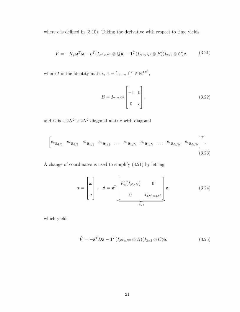
V = −KpωTω − eT (IN2×N2 ⊗Q)e− 1T (IN2×N2 ⊗B)(I2×2 ⊗ C)e, (3.21)

where I is the identity matrix, 1 = [1, ..., 1]T ∈ R4N2,

B = I2×2 ⊗

−1 0

0 ε

, (3.22)

and C is a 2N2 × 2N2 diagonal matrix with diagonal

[Bka1/1

Bka1/1Bka1/2

Bka1/2 . . . Bka1/NBka1/N . . . BkaN/N

BkaN/N

]T.

(3.23)

A change of coordinates is used to simplify (3.21) by letting

z =

ωe

, z = zT

Kp(IN×N) 0

0 I4N2×4N2

︸ ︷︷ ︸

,D

z, (3.24)

which yields

V = −zTDz− 1T (IN2×N2 ⊗B)(I2×2 ⊗ C)e. (3.25)

21

Note that the second term can be rewritten as the following double summation

N∑k=1

N∑j=1

BkaTj/k(4rj/k − ε4Bkvj/k

), (3.26)

where 4rj/k is the position error and 4Bkvj/k is the velocity error. In the context

of the problem, we assume that the relative position is measured. Therefore, in

steady-state, 4rj/k is proportional to the measurement noise, which we ignore.

This simplification allows the function of gains to be pulled outside of the double

summation and used to scale this term in the Lyapunov derivative. Under this

simplification, V ≤ 0 when

zTDz > εN∑k=1

N∑j=1

||BkaTj/k4Bkvj/k||. (3.27)

Hence, solutions that lie outside the bound zTDz = ε∑N

k=1

∑Nj=1 ||BkaTj/k4Bkvj/k||,

will approach this boundary. Once inside, solutions will remain there because V < 0

in the region outside of the boundary.

In this stability condition, we have some authority over ε through our choice of

estimator gains. Making ε small reduces the ultimate bound on z, allowing vehicles

to approach arbitrarily close to the parallel formation. Simulated results of the

parallel formation are displayed in Fig. 3.3.

Theorem 5. Choosing the control νk = γk(θk,Rk) defined in (2.4) guarantees that

along solutions of (3.15), z = [(ωT − ω01T ) eT ]T is bounded by a quantity propor-

tional to ε given in (3.10).

22

−30 −25 −20 −15 −10 −5 0

−15

−10

−5

0

5

10

x

y

(a) Trajectories

0 5 10 15 20 25 300

0.5

1

1.5

2

2.5

3

t(s)

||4r j

/k||

Error in Position Estimates

(b) Position Estimation Errors

0 5 10 15 20 25 300

5

10

15

20

25

30

t(s)

||4B k

vj/k||

Error in Velocity Estimates

(c) Velocity Estimation Errors

Figure 3.3: A simulation of five self-propelled vehicles performing the parallel controllaw using the observer-based feedback control algorithm. Each vehicle is given arandom initial position and velocity; K = −1, Kp = 1, K1 = 10, and K2 = 100.

Proof. Consider the following composite Lyapunov function

V = eT (IN2×N2 ⊗ P )e +KpKω

20

2trace(cTPc) +

1

2

N∑k=1

(ωk − ω0)2 (3.28)

where c = [c1, ..., cN ]T , Kp > 0, K > 0, and P is the projector matrix. The vector

e and matrix P are defined in (3.19) and (3.20), respectively. Taking the derivative

with respect to time yields

V = eT (IN2×N2 ⊗Q)e− 1T (IN2×N2 ⊗B)(I2×2 ⊗ C)e

−Kp(ω − ω01)T (ω − ω01), (3.29)

where ω = [ω1, ..., ωN ] and Q ∈ R4×4 is the identity matrix. The matrix B is defined

in (3.22). A change of coordinates is used to simplify (3.29) by letting

z =

ω − ω01

e

, z = zTDz, (3.30)

23

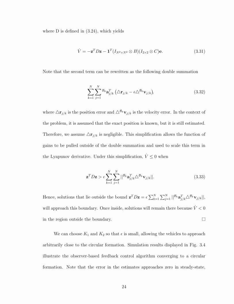
where D is defined in (3.24), which yields

V = −zTDz− 1T (IN2×N2 ⊗B)(I2×2 ⊗ C)e. (3.31)

Note that the second term can be rewritten as the following double summation

N∑k=1

N∑j=1

BkaTj/k(4rj/k − ε4Bkvj/k

), (3.32)

where 4rj/k is the position error and 4Bkvj/k is the velocity error. In the context of

the problem, it is assumed that the exact position is known, but it is still estimated.

Therefore, we assume 4rj/k is negligible. This simplification allows the function of

gains to be pulled outside of the double summation and used to scale this term in

the Lyapunov derivative. Under this simplification, V ≤ 0 when

zTDz > εN∑k=1

N∑j=1

||BkaTj/k4Bkvj/k||. (3.33)

Hence, solutions that lie outside the bound zTDz = ε∑N

k=1

∑Nj=1 ||BkaTj/k4Bkvj/k||,

will approach this boundary. Once inside, solutions will remain there because V < 0

in the region outside the boundary.

We can choose K1 and K2 so that ε is small, allowing the vehicles to approach

arbitrarily close to the circular formation. Simulation results displayed in Fig. 3.4

illustrate the observer-based feedback control algorithm converging to a circular

formation. Note that the error in the estimates approaches zero in steady-state,

24

which implies that each vehicle determines the relative position and relative velocity

of the other vehicles as time goes to infinity.

−4 −2 0 2 4 6

0

1

2

3

4

5

6

7

8

x

y

(a) Trajectories

0 20 40 60 80 1000

0.5

1

1.5

2

2.5

3

t(s)

||4r j

/k||

Error in Position Estimates

(b) Position Estimation Errors

0 20 40 60 80 1000

5

10

15

20

25

30

t(s)

||4B k

vj/k||

Error in Velocity Estimates

(c) Velocity Estimation Errors

Figure 3.4: A simulation of five self-propelled vehicles performing the circular controllaw using the observer-based feedback control algorithm with ω0 = 0.25. Eachvehicle is given a random initial position and velocity; K = 1, Kp = 1, K1 = 10,and K2 = 100.

With theoretical justification behind the observer-based feedback control al-

gorithm, the next step is to perform the derived control laws on a more realistic

system for validation. Before implementation on a miniature submarine platform

described in Chapter 5, a six degree of freedom model was constructed to mimic

the vehicle’s behavior. The cooperative control laws are then applied to this higher

fidelity model for analysis.

25

Chapter 4

Simulation Results

The vehicle model used above is useful in developing control laws, but does

not take into account the dynamics of a physical system performing that control.

Therefore, we have developed a higher fidelity model of our miniature submarine

that comprises our laboratory scale testbed. Simulation of this model provides a

prediction of the vehicle’s behavior before experimental testing is performed.

4.1 Six Degree of Freedom Submarine Model

This higher fidelity model is derived using an inertial frame and body frame.

The inertial frame, I = (O,gx,gy,gz), is affixed to the ground at point O with the

positive gz direction into the ground. The gx and gy directions can be arbitrarily

chosen, but must be constrained such that gx×gy = gz, to maintain a right-handed

coordinate system. The body fixed frame, B = (P,b1,b2,b3) is attached to the

body of the submarine at point P which coincides with the vehicle’s center of mass.

The principle axes of this frame are chosen according to aircraft convention such

that b1 is out the nose of the vehicle, b2 is out the right side, and b3 is out the belly

of the submarine.

With these frames defined, the forces on the body displayed in Fig. 4.1 can

26

Fb

Fg

Fr

(a) Front View

Fb

Fg

Fe

Ft

Fd

(b) Side View

Figure 4.1: Free-body diagram of submarine model

Submarine Properties

Mass(kg) Length(m) Width(m) Height(m) I1 (kg/m2) I2 (kg/m2) I3 (kg/m2)

7.79 0.991 0.165 0.165 0.212 0.393 0.393

S1 (m2) S2 (m2) S3 (m2) Se (m2) Sr (m2)

.0214 .128 .128 .0016 .0019

Table 4.1: Physical miniature submarine properties

be defined as

Fg = mggz

Fb = −ρwV ggz

Ft = 35utb1

Fd = −q∞1S1Cdb1 − q∞2S2Cdb2 − q∞3S3Cdb3

Fr = 2q∞1Sr sin(urπ/4)b2

Fe = 2q∞1Se sin(ueπ/4)b3

(4.1)

where F represents a force, u represents control input from -1 to 1, Cd is the drag

coefficient, m represents the vehicle’s mass, ρw is the density of water, V is the

volume of displaced water, and q∞ refers to the instantaneous dynamic pressure

27

along a particular direction of the body frame denoted by the subscript number.

The subscripts on the force and control terms refer to a specific force or input. In

this model, the subscript g refers to gravity, b to buoyancy, t to thrust, d to drag,

r to rudder, and e to the dive planes. The other terms in (4.1) relate to physical

properties of the vehicle and are defined in Table 4.1.

4.2 Numerical Integration of Submarine Model

The forces described above determine how the submarine model will translate

and rotate in time. More specifically, the translational and rotational equations of

motion for the submarine model obey Euler’s equations and are defined according

to aircraft convention with a 3-2-1 Euler angle rotation sequence [14]. Integration

of the twelve equations of motion produce the submarine’s position, velocity, body

rates, and Euler angles in time which are used to evaluate the vehicle’s performance.

The actual integration of these equations of motion was performed using a

first-order Euler integration scheme shown in (4.2) where t represents a specific

time and 4t represents the time step. The subscripted F ’s and M ’s refer to forces

and moments along the subscript’s frame direction, respectively. Although this

integration method may not be as accurate as other schemes, it allows for real-

time application of control signals at discrete intervals. These signals are provided

autonomously or via a user interface in real-time. This discrete application of control

is used to mimic our underwater-vehicle testbed control structure which runs at two

separate frequencies. Control to the submarine’s dive planes is provided at 20 Hz,

28

which is matched by the simulator exactly. The onboard rudder control runs at

50Hz, which is simulated at a slightly faster frequency of 60Hz. In addition to the

discrete control application, a visual framework is also used to provide the user with

continuous feedback.

x(t+4t) = x(t) + x4t

y(t+4t) = y(t) + y4t

z(t+4t) = z(t) + y4t

x(t+4t) = x(t) + (∑Fx/m)4t

y(t+4t) = y(t) + (∑Fy/m)4t

z(t+4t) = z(t) + (∑Fz/m)4t

φ(t+4t) = φ(t) + (w1 + ω2 sinφ tan θ + ω3 cosφ tan θ)4t

θ(t+4t) = θ(t) + (ω2 cosφ− ω3 sinφ)4t

ψ(t+4t) = ψ(t) + (ω2 sinφ+ ω3 cosφ) sec θ4t

ω1(t+4t) = ω1(t) +∑M1−(I3−I2)w2w3

I14t

ω2(t+4t) = ω2(t) +∑M2−(I1−I3)w1w3

I24t

ω3(t+4t) = ω3(t) +∑M3−(I2−I1)w1w2

I34t

(4.2)

These equations of motion define the submarine’s movement in a three-dimensional

world. Collective behaviors such as spirals and circular formations on the surface of

a sphere [5] exist in this higher degree of freedom world. However, the cooperative

control algorithms in this paper have been designed for a planar case. Therefore, the

submarine model will need to implement a depth controller to constrain a transla-

tional degree of freedom. Once depth is stabilized, the cooperative control algorithm

29

resembles the planar case with the submarine’s yaw angle equivalent to the planar

velocity orientation.

Stabilization of depth is achieved using a proportional-integral controller on

the error between the vehicle’s actual and desired depth. A simple proportional

controller will not be effective in this case, because an offset in the dive planes is

required to provide a counteracting force opposing the buoyancy force. The integral

term determines the required offset and stabilizes the system with respect to depth.

4.3 Simulated Cooperative Control Algorithms

The simulation architecture for the submarine model runs on an object-oriented

programming language, which allows the submarine model to be replicated to N

identical vehicles used to test the cooperative control laws. We begin by testing

the parallel and circular control laws without estimation defined in (2.2) and (2.4).

Validation of these control laws is essential before testing the more complex observer-

based feedback control algorithm, which is built upon its predecessor. In addition

to having the formation converge, we are also interested in seeing that the other

states of the model remain stable.

4.3.1 Parallel & Circular Control

In order to perform the cooperative control laws defined in Chapter 2, some

modifications to these laws are necessary. For the parallel control law, the vehicle

model assumes that the relative velocity orientation between vehicles is known.

30

Our physical testbed cannot directly measure the velocity of the submarines, but it

can tell us the position and pose of the vehicle. With this knowledge, we assume

that the submarine’s velocity aligns with the orientation of the body. Although

this assumption is generally not true, vehicles traveling in a straight line will not

exhibit any sideslip angle. Therefore, submarines in a parallel formation should each

maintain a zero sideslip angle as well. Under this assumption, the control law in

(2.6) becomes

uk = Kp(αk(ψ)− ωk), (4.3)

where ψk = [ψ1 − ψk, ..., ψN − ψk]T .

Note that the yaw angles ψk, are used to determine the relative velocity orien-

tation. The yaw angles are used because they are equivalent to velocity orientation

in the planar case when depth is managed. A five vehicle simulation of this control

law is shown from an overhead view in Fig. 4.2. Note that just like the parti-

cle model, each submarine is able to converge to the desired formation with little

oscillation about the final direction.

This simulation displays that the submarine models are able to manage depth

as well as perform the collective behavior. In addition to achieving this goal, each

vehicle’s body rates and velocities reach a constant value as t→∞. These constant

values imply that each vehicle reaches a stable steady-state behavior and will remain

there.

Similar to the parallel control law, the circular control law requires some slight

modifications before implementation. The assumption that the submarine’s yaw

31

−50 −40 −30 −20 −10 0

−35

−30

−25

−20

−15

−10

−5

0

5

x(m)

y(m)

z(m)

−3

−2.5

−2

−1.5

−1

−0.5

0

0 10 20 30 40 50 60

−40

−20

0Positions vs. Time

t(s)

x(m

)

0 10 20 30 40 50 60

−30−20−10

0

t(s)

y(m)

0 10 20 30 40 50 60−3

−2

−1

0

t(s)

z(m)

zd

0 10 20 30 40 50 60

−0.8−0.6−0.4−0.2

00.20.4

Velocities vs. Time

t(s)

x(m

/s)

0 10 20 30 40 50 60

−0.5

0

0.5

t(s)

y(m/s)

0 10 20 30 40 50 60

−0.2

0

0.2

t(s)

z(m/s)

0 10 20 30 40 50 60−0.04

−0.02

0

0.02

Euler Angles vs. Time

t(s)

Roll(rad)

0 10 20 30 40 50 60

−0.4

−0.2

0

0.2

t(s)

Pitch

(rad)

0 10 20 30 40 50 60

2

3

4

5

t(s)

Yaw

(rad)

0 10 20 30 40 50 60

−0.02

0

0.02

Body Rates vs. Time

t(s)

ω1(rad/s)

0 10 20 30 40 50 60−0.2

−0.1

0

0.1

t(s)

ω2(rad/s)

0 10 20 30 40 50 60

−0.1

0

0.1

t(s)

ω3(rad/s)

Figure 4.2: A simulation of five submarine models performing the parallel controllaw; K = −1 and Kp = 1.

32

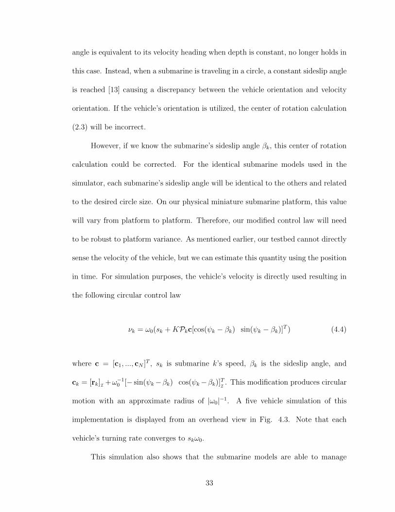
angle is equivalent to its velocity heading when depth is constant, no longer holds in

this case. Instead, when a submarine is traveling in a circle, a constant sideslip angle

is reached [13] causing a discrepancy between the vehicle orientation and velocity

orientation. If the vehicle’s orientation is utilized, the center of rotation calculation

(2.3) will be incorrect.

However, if we know the submarine’s sideslip angle βk, this center of rotation

calculation could be corrected. For the identical submarine models used in the

simulator, each submarine’s sideslip angle will be identical to the others and related

to the desired circle size. On our physical miniature submarine platform, this value

will vary from platform to platform. Therefore, our modified control law will need

to be robust to platform variance. As mentioned earlier, our testbed cannot directly

sense the velocity of the vehicle, but we can estimate this quantity using the position

in time. For simulation purposes, the vehicle’s velocity is directly used resulting in

the following circular control law

νk = ω0(sk +KPkc[cos(ψk − βk) sin(ψk − βk)]T ) (4.4)

where c = [c1, ..., cN ]T , sk is submarine k’s speed, βk is the sideslip angle, and

ck = [rk]I +ω−10 [− sin(ψk−βk) cos(ψk−βk)]TI . This modification produces circular

motion with an approximate radius of |ω0|−1. A five vehicle simulation of this

implementation is displayed from an overhead view in Fig. 4.3. Note that each

vehicle’s turning rate converges to skω0.

This simulation also shows that the submarine models are able to manage

33

−6 −4 −2 0 2 4

−5

−4

−3

−2

−1

0

1

2

3

4

x(m)

y(m)

z(m)

−3

−2.5

−2

−1.5

−1

−0.5

0

0 20 40 60 80 100 120−6−4−202

Positions vs. Time

t(s)

x(m

)

0 20 40 60 80 100 120

−4−2024

t(s)

y(m)

0 20 40 60 80 100 120−3

−2

−1

0

t(s)

z(m)

zd

0 20 40 60 80 100 120

−0.5

0

0.5

Velocities vs. Time

t(s)

x(m

/s)

0 20 40 60 80 100 120

−0.5

0

0.5

t(s)

y(m/s)

0 20 40 60 80 100 120

−0.2

0

0.2

t(s)

z(m/s)

0 20 40 60 80 100 120−0.3

−0.2

−0.1

0

Euler Angles vs. Time

t(s)

Roll(rad)

0 20 40 60 80 100 120−0.4

−0.2

0

t(s)

Pitch

(rad)

0 20 40 60 80 100 120

10

20

30

t(s)

Yaw

(rad)

0 20 40 60 80 100 120

0

0.1

0.2Body Rates vs. Time

t(s)

ω1(rad/s)

0 20 40 60 80 100 120−0.2

−0.1

0

0.1

t(s)

ω2(rad/s)

0 20 40 60 80 100 120

−0.5

0

0.5

t(s)

ω3(rad/s)

Figure 4.3: A simulation of five submarine models performing the circular controllaw; K = 1 and Kp = 1.

34

depth as well as perform circular trajectories. In addition to collective motion,

each submarine’s steady-state behavior suggests that the platform is stable. With

validation that both parallel and circular control laws are stable onboard the higher

fidelity model, simulation of the observer-based feedback control algorithm can be

performed.

4.3.2 Observer-Based Feedback Control

In order to perform the observer-based feedback control algorithm, every sub-

marine needs to maintain estimates for every other model in their own path frame.

This estimation is achieved by integrating (3.9) with a first-order Euler integration

scheme with respect to the vehicle’s path frame that is aligned with the submarine’s

velocity. With these estimates defined, the relative velocity orientation is computed,

followed by the control algorithms described above. Note that both collective al-

gorithms no longer require that each vehicle has knowledge of every other vehicle’s

velocity orientation or sideslip angle because the estimates provide that information.

However, implementation of the control algorithm onboard a vehicle still requires

knowledge of that vehicle’s own velocity orientation or sideslip angle.

Simulations of this control onboard the submarine model have often displayed

an oscillatory behavior around the desired trajectory with identical control gains

used on the vehicle model. These oscillatory motions are illustrated in Fig. 4.4.

When examining the errors in the estimated position and velocity, we notice that

they do not converge to zero, but rather, are bounded according to Lemma 3.

35

−25 −20 −15 −10 −5 0 5 10 15 20

−5

0

5

10

15

20

25

30

x(m)

y(m

)

0 5 10 15 20 25 300

0.5

1

1.5

2

2.5

3

t(s)

||4r j

/k||

Error in Position Estimates

0 5 10 15 20 25 300

5

10

15

20

25

30

t(s)

||4B k

vj/k||

Error in Velocity Estimates

−12 −10 −8 −6 −4 −2 0 2 4 6−10

−8

−6

−4

−2

0

2

4

6

x(m)

y(m

)

(a) Trajectories

0 20 40 60 80 100 1200

0.5

1

1.5

2

2.5

3

t(s)

||4r j

/k||

Error in Position Estimates

(b) Position Estimation Errors

0 20 40 60 80 100 1200

5

10

15

20

25

30

t(s)

||4B k

vj/k||

Error in Velocity Estimates

(c) Velocity Estimation Errors

Figure 4.4: Simulations of five submarine models performing the observer-basedfeedback control algorithm in which they exhibit oscillatory behavior; K1 = 10 andK2 = 100.

Understanding that the oscillation is a result of the perturbation term in the

estimator dynamics, gives us some options as to how to further reduce the impact

of this term. Based on theory, reducing ε should allow the formation to come

arbitrarily close to the particular formations as discussed in Theorems 4 and 5.

Small reductions in ε require that the choice of K2 increase dramatically. This gain

choice is not a valid option for our Euler integration scheme, which has a greater

probability of approaching instability the higher K2 becomes.

Therefore, instead of altering the estimator gains, K can be chosen to slow

down the convergence of the system. In addition to slowing down the formation,

K will decrease the vehicle’s turning rate, and ultimately reduce the time varying

perturbation gj/k(t), in which the turning rate is embedded.

36

For a parallel formation, simply reducing K is not sufficient because the per-

turbation also increases proportional to the distance between vehicles. This relation-

ship makes sense intuitively because slight variations in velocity orientation would

be harder to extract from larger distances. For example, imagine sitting on a beach

and watching a cargo ship in the distance. Determining its exact velocity orientation

by watching it move, is not a trivial calculation. Our problem goes one step further

in which the observer is not stationary, but is free to translate and rotate. Taking

this point into consideration, a scheduled gain choice of K = 9.99||pθ|| − 10 was

implemented onboard the model where pθ represents the alignment of the system

using velocity orientation estimates. When the vehicles are in a balanced forma-

tion, ||pθ|| = 0, creating a large K gain. This large gain causes the submarines to

converge quickly. When the collective is in a parallel formation, ||pθ|| = 1, creating

a small K gain. This gain choice reduces the speed of convergence as well as the

rotational movement of the model. The reduction allows the estimates to converge,

and ultimately, the formation converges as well, as indicated in Fig. 4.5.

0 20 40 60 80 100 120

−10

0

10

20

30

40

50

60

70

80

x(m)

y(m

)

(a) Trajectories

0 50 100 1500

0.5

1

1.5

2

2.5

3

t(s)

||4r j

/k||

Error in Position Estimates

(b) Position Estimation Errors

0 50 100 1500

5

10

15

20

25

30

t(s)

||4B k

vj/k||

Error in Velocity Estimates

(c) Velocity Estimation Errors

Figure 4.5: A simulation of five submarine models performing the scheduled parallelcontrol law; K = 9.99||pθ|| − 10, Kp = 1, K1 = 10, and K2 = 100.

For circular motion, reducing K alone allows the formation to approach the

37

circular formation as displayed in Fig. 4.6. Although there is still slight error in the

estimates, the general circular pattern of the formation is reproduced. Controllers

with scheduled gains have also been implemented on this model, altering the gain

K as a function of how close the vehicles’ centers of rotation are aligned. These

simulations produced very similar results as those shown in Fig 4.6.

−12 −10 −8 −6 −4 −2 0 2 4 6 8

−8

−6

−4

−2

0

2

4

6

x(m)

y(m

)

(a) Trajectories

0 20 40 60 80 100 1200

0.5

1

1.5

2

2.5

3

t(s)

||4r j

/k||

Error in Position Estimates

(b) Position Estimation Errors

0 20 40 60 80 100 1200

5

10

15

20

25

30

t(s)

||4B k

vj/k||

Error in Velocity Estimates

(c) Velocity Estimation Errors

Figure 4.6: A simulation of five submarine models performing the circular controllaw with small alignment gain and ω0 = 0.25; K = .1 Kp = 1, K1 = 10, andK2 = 100.

38

Chapter 5

Experimental Results

As previously mentioned, the proposed control laws have been designed for

an idealized model that does not take into account the individual dynamics of a

physical platform. Validation of these control algorithms is achieved through the

implementation of closed-loop control onboard a testbed of miniature submarines.

More specifically, each submarine’s trajectory is recorded and compared against the

formation that should emerge. Submarine trajectories that coincide with the vehicle

model validate that the control law is a viable option for similar platforms.

5.1 Underwater-Vehicle Testbed

The submarines used in the testbed are 1:60 scale models of the U.S.S. Alba-

core which have been modified to operate via remote control as shown in Fig. 5.1.

Inside each vehicle’s hull are two separate pressure vessels. The smaller vessel at the

nose of the craft is used as the battery compartment. Behind that enclosure lies the

main pressure vessel which houses the electronics as displayed in Fig 5.2. The vessels

have an insulated wire connection between them providing power to the electronics.

The two-pressure vessel design allows the main pressure vessel’s water-tight seal to

remain intact, while swapping out used batteries for new ones.

Although the submarine is a replica of the U.S.S. Albacore, the model does

39

Figure 5.1: Miniature submarine models of the U.S.S. Albacore that comprise theunderwater vehicle testbed

not utilize a ballast system to regulate depth. Instead, the submarine is described as

a dynamic diver because it uses its velocity and dive planes to remain underwater.

Under this classification, the vehicle is weighted close to neutral buoyancy, but

slightly positive. This choice in buoyancy allows the dive planes to be more effective

since they have to counteract a small rising force. In addition, the weighting of the

submarine allows for surfacing by simply turning off the propeller in emergencies.

Communication to the vehicle is provided by a 72Mhz radio transmitter and

receiver. The transmitter and corresponding receiver utilize a matching crystal that

allows control signals to be passed from the transmitter to the receiver. The crystals

are manufactured in several channels, which allow multiple vehicles to function at

the same time without interference. In application, the wireless communication

functions to a depth of approximately 3 meters. Once that depth is surpassed,

the signal attenuates and the connection is broken. This signal loss initializes the

motor’s failsafe mechanism, stopping the propeller. The submarine then rises back

into communication range where control is resumed.

In its current configuration, the submarine is designed to operate under human

40

Submarine Connections

5V Signal Wire

12V Power Line

Mechanical Linkage

Dive Planes

Rudder

Propeller

Servo

Battery MotorReceiverSpeed

Controller

Servo

Figure 5.2: Wiring diagram for remote operation

control. Altering the vehicle’s setup to an autonomous configuration is achieved in

two stages. The first stage is accomplished by adding a microcontroller onboard each

vehicle. More specifically, an arduIMU+ board [1] is affixed inside the main pres-

sure vessel. This board contains three accelerometers and three gyroscopes aligned

along three orthogonal axes. In addition to its sensing capability, a programmable

ATMEGA328 chip is used to poll these sensors inside of a customizable control loop.

In our submarine, this board is placed between the receiver and servo, which

controls the rudder as illustrated in Fig. 5.3. The receiver provides the board with

power and a pulse width modulation signal. In standard operation, the servo inter-

prets this signal and rotates to a prescribed angle defined by the width of the pulse.

In the autonomous configuration, the pulse width is read by the microcontroller

and is linearly mapped to a desired yaw rate. This rate is used in a proportional

state feedback controller with the yaw rate gyroscope. The resulting control signal

41

Submarine Connections

5V Signal Wire

12V Power Line

Mechanical Linkage

Dive Planes

Rudder

Propeller

Servo

Battery MotorReceiverSpeed

Controller

Servo

ArduIMU+

Figure 5.3: Wiring diagram for autonomous operation

from this calculation is linearly mapped back to a pulse width. This new signal

is then passed to the servo and rotates the rudder. Pseudocode for this control

implementation is shown in Fig. 5.4.

The addition of the microcontroller to the submarine alters the functionality of

the rudder control stick on the transmitter. Rather than controlling the deflection

of the rudder, the user now controls a desired turning rate for the vehicle. The

arduIMU+ board closes the loop and stabilizes the yaw rate within the physical

limitations of the vehicle. With the submarine’s yaw rate stabilized by control, the

second stage to autonomous operation removes the user from the control loop via

the transmitter’s trainer port. The trainer port is typically used to teach another

individual how to operate the vehicle. In this case, the trainer gives control of

the submarine to a trainee’s transmitter by engaging a switch located on his own

transmitter. When disengaging the switch, the trainer takes back control of the

42

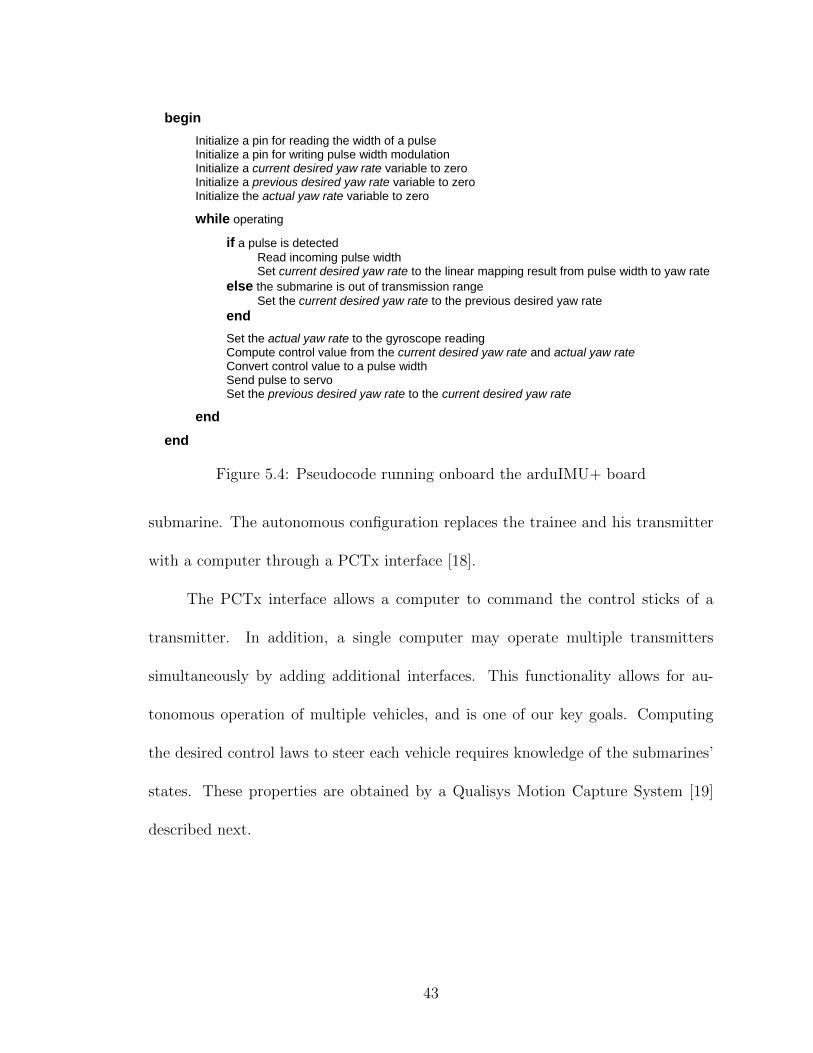
begin

Initialize a pin for reading the width of a pulse Initialize a pin for writing pulse width modulation Initialize a current desired yaw rate variable to zero Initialize a previous desired yaw rate variable to zero Initialize the actual yaw rate variable to zero

while operating

if a pulse is detected

Read incoming pulse width Set current desired yaw rate to the linear mapping result from pulse width to yaw rate;

else the submarine is out of transmission range

Set the current desired yaw rate to the previous desired yaw rate

end

Set the actual yaw rate to the gyroscope reading Compute control value from the current desired yaw rate and actual yaw rate Convert control value to a pulse width Send pulse to servo Set the previous desired yaw rate to the current desired yaw rate

end

end

Figure 5.4: Pseudocode running onboard the arduIMU+ board

submarine. The autonomous configuration replaces the trainee and his transmitter

with a computer through a PCTx interface [18].

The PCTx interface allows a computer to command the control sticks of a

transmitter. In addition, a single computer may operate multiple transmitters

simultaneously by adding additional interfaces. This functionality allows for au-

tonomous operation of multiple vehicles, and is one of our key goals. Computing

the desired control laws to steer each vehicle requires knowledge of the submarines’

states. These properties are obtained by a Qualisys Motion Capture System [19]

described next.

43

5.2 Qualisys Motion Capture System

The Qualisys Motion Capture System utilizes twelve underwater cameras to

track the position of retroreflective markers. Six markers are affixed to the hull

of each submarine in different, varying configurations. The motion capture sys-

tem defines rigid bodies based on the placement of the markers with respect to

their counterparts. The varying configurations are required so that the system can

track multiple vehicles. As long as three markers are tracked by the system, the

submarine’s position and pose can be calculated. It is important to note that the

placement of markers with similar or symmetric patterns will confuse the system’s

interpretation of the rigid bodies, resulting in poor tracking.

(a) Cameras (b) Isometric View (c) Top View

Figure 5.5: Qualisys Motion Capture System

With well-defined placement of markers for our submarine models, tracking

their position and pose can be achieved in real-time with the provided source code.

In addition to polling this data at 20Hz, the system can also record the vehicle’s

motion for postprocessing. As mentioned in Chapter 4, the system can only pro-

vide the vehicle’s position and pose. However, some control implementations re-

quire knowledge of the vehicle’s velocity direction and turning rate. These values

44

are determined via a differencing approach between measurements. Although the

estimation method is influenced by tracking losses, the estimates are required to

compute the desired control.

With measurements available to perform the control laws, the automation loop

can be closed by combining the Qualisys and PCTx source codes. The autonomous

control loop starts by retrieving the states of each vehicle being tracked. The control

laws use these states to determine an elevator deflection and desired turning rate for

each vehicle based on the control laws. These control signals are then passed down

to the submarines through the PCTx interface, closing the loop. Fig. 5.6 displays

the control architecture discussed above.

Qualisys

Yaw Rate Gyroscope

Turning Rate Controller

Depth Controller

Cooperative Control Law

Onboard Control Loop: 50Hz

Topside Control Loop: 20Hz

+

+

-

-

Submarine

Figure 5.6: Control architecture for the underwater vehicle testbed.

45

5.3 Experimental Results of the Underwater Vehicle Testbed

The autonomous vehicle design discussed above was installed in the Neutral

Buoyancy Research Facility at the University of Maryland, College Park. The

testbed operates within the tank, which is 25 feet deep and 50 feet across, and

is also equipped with twelve Qualisys underwater cameras. Camera placement is

crucial for maximizing the capture volume which is shown in Fig. 5.5.

With this control architecture in place, validation of the cooperative control

laws can be achieved. To begin testing, a single submarine combined with a virtual

vehicle in the tank is used. The virtual vehicle is unaware of the submarine in

the tank and holds its current parallel or circular formation. The submarine is

able to ”see” the virtual vehicle and computes the desired control with the virtual

vehicle, being part of its group. This distinction allows the virtual vehicle to steer

the submarine to a preset formation, because its control is independent of the other

vehicles in the group [22].

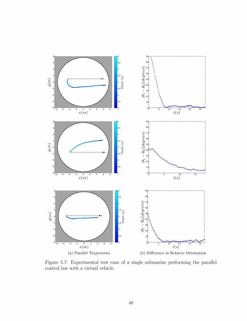
5.3.1 Virtual Vehicle Experiments

In parallel experiments, the virtual vehicle travels along the positive x axis of

the tank. In theory, the submarine should minimize the relative orientation angle

between the virtual vehicle and itself, resulting in both vehicles traveling along the

same direction. Fig. 5.7 shows three experimental tests of this particular formation.

Note that in each experimental run, the submarine begins with a large error in

relative orientation angle; but, by the time it reaches the edge of the tank, the

46

difference is minimal. Although theory and simulation demonstrate that the relative

orientation between vehicles goes to zero, we do anticipate slight oscillations about

this point due to sensor noise in the system. Based on these test runs, parallel control

with a virtual vehicle is validated because phase synchronization was achieved by

the submarine, repeatedly.

With the parallel formation validated, we continue the virtual vehicle experi-

ments with the circular formation. The circular control law was implemented with

a virtual vehicle circling the center of the tank with a radius of 2.5 meters. In this

case, we accounted for the submarine’s velocity heading not being aligned with the

orientation of the rigid body by the estimation discussed earlier. In the experimental

test runs, the submarine starts around the virtual vehicle’s circular trajectory and

begins to encircle the center of the tank as shown in Fig. 5.8. The radius of the

circle traced out by the submarine does not match the radius of the virtual vehicle

exactly; however, the submarine does stabilize to a constant offset of approximately

0.1 meters. The error in the centers of rotation is attributed to the measurement

noise being neglected in our calculations. Similar to the parallel formation, these

experimental tests validate that the circular formation is feasible for implementation

on a physical platform.

5.3.2 Multi-Vehicle Experiments

With validation of a single submarine’s capability to perform the desired mo-

tion completed, multi-vehicle experiments were then conducted. For this configura-

47

−8 −6 −4 −2 0 2 4 6 8−8

−6

−4

−2

0

2

4

6

8

x(m)

y(m

)

Depth

(m)

0

0.5

1

1.5

2

2.5

3

3.5

40 5 10 15 20 25

0

10

20

30

40

50

60

70

80

90

t(s)

|θ 1−θ 0|(d

egrees)

−8 −6 −4 −2 0 2 4 6 8−8

−6

−4

−2

0

2

4

6

8

x(m)

y(m

)

Depth

(m)

0

0.5

1

1.5

2

2.5

3

3.5

40 5 10 15

0

10

20

30

40

50

60

70

80

90

t(s)

|θ 1−θ 0|(d

egrees)

−8 −6 −4 −2 0 2 4 6 8−8

−6

−4

−2

0

2

4

6

8

x(m)

y(m

)

Depth

(m)

0

0.5

1

1.5

2

2.5

3

3.5

4

(a) Parallel Trajectories

0 5 10 15 20 250

10

20

30

40

50

60

70

80

90

t(s)

|θ 1−θ 0|(d

egrees)

(b) Difference in Relative Orientation

Figure 5.7: Experimental test runs of a single submarine performing the parallelcontrol law with a virtual vehicle.

48

−8 −6 −4 −2 0 2 4 6 8−8

−6

−4

−2

0

2

4

6

8

x(m)

y(m

)

Depth

(m)

0

0.5

1

1.5

2

2.5

3

3.5

40 20 40 60 80 100 120 140 160

0

5

10

15

t(s)

||c1−c0||(m)

−8 −6 −4 −2 0 2 4 6 8−8

−6

−4

−2

0

2

4

6

8

x(m)

y(m

)

Depth

(m)

0

0.5

1

1.5

2

2.5

3

3.5

40 20 40 60 80 100

0

5

10

15

t(s)

||c1−c0||(m)

−8 −6 −4 −2 0 2 4 6 8−8

−6

−4

−2

0

2

4

6

8

x(m)

y(m

)

Depth

(m)

0

0.5

1

1.5

2

2.5

3

3.5

4

(a) Circular Trajectories

0 10 20 30 40 50 600

5

10

15

t(s)

||c1−c0||(m)

(b) Error in Centroid Position

Figure 5.8: Experimental test runs of a single submarine performing the circularcontrol law with a virtual vehicle.

49

tion, we remove the virtual vehicle, allowing the submarines to collectively decide

their overall formation. The resulting formation is determined by the initial condi-

tions and vehicle dynamics. Utilizing the vehicle and submarine model, final vehicle

trajectories can be predicted given their initial conditions. Using this knowledge,

the initial conditions of the submarines were contrived to optimize the use of the

tank.

For the parallel formation, two submarines were started within close proximity

to each other with orientation differences ranging from 30 to 55 degrees as shown

in Fig. 5.9. Two submarines will minimize this difference by rotating toward each

other until they have reached a parallel formation. The three experimental tests

performed, indicate that the control law is operating as we would expect, but with

larger errors than those seen by the the virtual vehicle experiments. This decline

in performance is anticipated, because the virtual vehicle experiments had complete

control of one vehicle, not corrupted by sensor noise. Adding the second submarine

creates additional noise as well as the complexity of another vehicle’s dynamics to

the problem. However, even with the vehicle addition, the parallel behavior still

emerges.

In similar fashion, the circular control was also tested with two submarines as

shown in Fig. 5.10. Initial conditions were contrived using the vehicle and submarine

models to have the final trajectories remain around the center of the tank. In these

tests, the submarines are trying to stabilize around the same circle with a 3 meter

radius. In comparison to the virtual vehicle experiments, these tests, in general,

fair worse. However, the results do show promising behavior in that the vehicles

50

−8 −6 −4 −2 0 2 4 6 8−8

−6

−4

−2

0

2

4

6

8

x(m)

y(m

)

Depth

(m)

0

0.5

1

1.5

2

2.5

3

3.5

40 2 4 6 8 10 12

0

10

20

30

40

50

60

70

80

90

t(s)

|θ 2−θ 1|(d

egrees)

−8 −6 −4 −2 0 2 4 6 8−8

−6

−4

−2

0

2

4

6

8

x(m)

y(m

)

Depth

(m)

0

0.5

1

1.5

2

2.5

3

3.5

40 2 4 6 8 10

0

10

20

30

40

50

60

70

80

90

t(s)

|θ 2−θ 1|(d

egrees)

−8 −6 −4 −2 0 2 4 6 8−8

−6

−4

−2

0

2

4

6

8

x(m)

y(m

)

Depth

(m)

0

0.5

1

1.5

2

2.5

3

3.5

4

(a) Parallel Trajectories

0 2 4 6 80

10

20

30

40

50

60

70

80

90

t(s)

|θ 2−θ 1|(d

egrees)

(b) Difference in Relative Orientation

Figure 5.9: Experimental test runs of two submarines performing the parallel controllaw.

51

−8 −6 −4 −2 0 2 4 6 8−8

−6

−4

−2

0

2

4

6

8

x(m)

y(m

)

Depth

(m)

0

0.5

1

1.5

2

2.5

3

3.5

40 2 4 6 8 10

0

5

10

15

t(s)

||c2−c1||(m)

−8 −6 −4 −2 0 2 4 6 8−8

−6

−4

−2

0

2

4

6

8

x(m)

y(m

)

Depth

(m)

0

0.5

1

1.5

2

2.5

3

3.5

40 5 10 15 20 25

0

5

10

15

t(s)

||c2−c1||(m)

−8 −6 −4 −2 0 2 4 6 8−8

−6

−4

−2

0

2

4

6

8

x(m)

y(m

)

Depth

(m)

0

0.5

1

1.5

2

2.5

3

3.5

4

(a) Circular Trajectories

0 5 10 15 20 250

5

10

15

t(s)

||c2−c1||(m)

(b) Error in Centroid Position

Figure 5.10: Experimental test runs of two submarines performing the circular con-trol law.

52

are rotating in the correct direction and the centroid difference doesn’t appear to

be growing. These findings give us reason to think that these trajectories are still

feasible, but may require additional modifications to the control algorithm.

5.3.3 Observer-Based Feedback Control Experiments

The testing of one and two vehicle systems above with the parallel (2.2) and

circular (2.4) control laws have been implemented to show they can be achieved

onboard a physical submarine. This testing was also completed to show that the

control laws are feasible in a case when all the states are able to be measured. If

the formation converges, we have reason to think that the observer-based feedback

control algorithm can stabilize the formation as well.

For the parallel experiments described above, it has been realized that the sub-

marines are a viable platform for implementation of the parallel control law. With

this point in mind, the observer-based feedback control algorithm was implemented

producing the following trajectory shown in Fig. 5.11. The addition of the observer

appears to slightly degrade the performance when compared to the two submarine

case. All in all, both submarines are traveling in, roughly, the same direction by the

time they reach the edge of the tank.

The observer-based method was also implemented with the circular control

law, with mixed results. Fig. 5.12 shows a test run of this case, where the perfor-

mance is similar to the two submarine test of the circular control law. Again, we

see each vehicle turning in the correct direction overall, but the difference in the

53

centroid appears to vary in time. Further study into this formation needs to be

completed to provide more viable trajectories.

−8 −6 −4 −2 0 2 4 6 8−8

−6

−4

−2

0

2

4

6

8

x(m)

y(m

)

Depth

(m)

0

0.5

1

1.5

2

2.5

3

3.5

4

(a) Parallel Trajectory

0 2 4 6 8 100

10

20

30

40

50

60

70

80

90

t(s)

|θ 2−θ 1|(d

egrees)

(b) Difference in Relative Orientation

Figure 5.11: Experimental test run of two submarines performing the parallel controllaw using the observer-based feedback control algorithm.

−8 −6 −4 −2 0 2 4 6 8−8

−6

−4

−2

0

2

4

6

8

x(m)

y(m

)

Depth

(m)

0

0.5

1

1.5

2

2.5

3

3.5

4

(a) Circular Trajectory

0 5 10 15 20 25 30 35 40 450

5

10

15

t(s)

||c2−c1||(m)

(b) Difference in Centroid Position

Figure 5.12: Experimental test run of two submarines performing the circular controllaw using the observer-based feedback control algorithm.

With all experimental tests completed and graphed, we conclude that a single

submarine performing the parallel or circular control law with a virtual vehicle is a

valid option for implementation on similar vehicles. In both cases, performance of

the desired motion was consistently achieved with varying initial conditions. As for

54

multi-vehicle testing, we conclude that the parallel formation is a valid option for

implementation with and without the observer. Results have indicated a slight loss

of performance, as the complexity of the algorithm increases; however, the overall

behavior can still be extracted. For circular formations, further research needs

to be conducted with regard to the combination of vehicle dynamics and control.

Finally, current results, although we are unable to validate these control algorithms,

do indicate that the formation is worth further examination due to the successful

virtual vehicle case.

55

Chapter 6

Conclusion & Future Work

6.1 Conclusion

This paper describes an observer-based feedback control algorithm to stabilize

parallel and circular formations. The proposed algorithm is theoretically justified for

a second-order vehicle model, and simulations illustrate convergence to the desired

formation. In addition, the cooperative control algorithms are extended to a three-

dimensional rigid-body submarine model that obeys Euler’s laws. Simulations using

this model reinforce the theoretical results obtained by the idealized version. A

laboratory scale testbed of underwater vehicles is also described in detail along with

corresponding experimental results. Test runs using a virtual vehicle validate the

parallel and circular control laws’ ability to stabilize to a desired formation. Multi-

vehicle testing of the cooperative control algorithms is also presented.

6.2 Future Work

Throughout this paper, we analyzed collective control algorithms on a simpli-

fied vehicle model. Using this framework, a generic algorithm can be designed and

applied to a variety of vehicles which mimic the behavior of the model. This control

design process excludes the specific vehicle dynamics which ultimately determine

56

how the vehicle will operate autonomously. Although this concept is addressed by

making modifications to the control law, designing the control around a specific

model should also be researched. It is our hope that research in this area could pro-

duce a more stable version of the cooperative control algorithm with better overall

performance.

In addition to this task, implementation of control has assumed that our sen-

sors have zero noise. In general, this is not true because every sensor contains some

inherent noise and may even be biased to some degree. This problem should be

addressed in a stochastic formulation to describe how noise influences the vehicle’s

performance.

Also, consider the linear estimator that was used in our research to determine

the relative velocity from one vehicle to another. Although the implementation of

this estimator is straight-forward, it comes at a cost. This paper has indicated

that the time-varying perturbation of this particular estimator greatly influences

the stability of the system. Other estimation techniques for determining relative

velocity should be researched to determine if they provide improved results. More

specifically, nonlinear estimators such as the extended Kalman filter, could offer

better estimates since the relative velocity does not vary linearly.

Lastly, experimental results in this paper began with a single submarine and

a virtual particle. Tests were extended to the case where two submarines performed

the cooperative motion. Future work should involve the implementation of control

on larger groups of submarines as well as other platforms that can operate outside

the testing facility. Vehicles fitting this profile can be used to demonstrate the value

57

of performing autonomous collective behaviors.

58

Bibliography

[1] Ardu-imu: Arduino based IMU & AHRS. http://code.google.com/p/

ardu-imu/wiki/Home, July 2011.

[2] Yongcan Cao, Wei Ren, and Ziyang Meng. Decentralized finite-time slidingmode estimators and their applications in decentralized finite-time formationtracking. Systems and Control Letters, 59(9):522–529, 2010.

[3] Wei Ding, Gangfeng Yan, and Zhiyun Lin. Collective motions and formationsunder pursuit strategies on directed acyclic graphs. Automatica, 46(1):174–181,2010.

[4] A. J. Healey. Application of formation control for multi-vehicle roboticminesweeping. Proceedings of the 40th IEEE Conference on Decision and Con-trol, 2:1497–1502, Orlando, Florida, 2001.

[5] S. Hernandez and D. A. Paley. Three-dimensional motion coordination in a spa-tiotemporal flowfield. IEEE Transactions on Automatic Control, 55(12):2805–2810, 2010.

[6] C H Hsieh, D Marthaler, B Q Nguyen, D J Tung, A L Bertozzi, and R MMurray. Experimental validation of an algorithm for cooperative boundarytracking. Proceedings of the American Control Conference, 2:1078–1083, 2005.

[7] N. J. Kasdin and D. A. Paley. Engineering Dynamics: A Comprehensive In-troduction. Princeton University Press, 1st. edition, 2011.

[8] H. Khalil. Nonlinear Systems. Prentice Hall, Upper Saddle River, NJ 07458,3rd. edition, 2002.

[9] Daniel J. Klein, Patrick K. Bettale, Benjamin I. Triplett, and Kristi A. Mor-gansen. Autonomous underwater multivehicle control with limited communica-tion: Theory and experiment. 2008.

[10] Naomi Ehrich Leonard, Derek A. Paley, Francois Lekien, Rodolphe Sepulchre,David M. Fratantoni, and Russ E. Davis. Collective motion, sensor networks,and ocean sampling. Proceedings of the IEEE, 95(1):48–74, 2007.

[11] Po-Hsiung Lin. The first successful typhoon eyewall-penetration reconnaissanceflight mission conducted by the unmanned aerial vehicle, aerosonde. Bulletinof the American Meteorological Society, 87(11):1481–1483, 2006.

[12] R. Mellish, S. Napora, and D. A. Paley. Backstepping control design for motioncoordination of self-propelled vehicles in a flowfield. International Journal ofRobust and Nonlinear Control, 21(12):1452–1466, 2011.

59

[13] R. Mellish and D. A. Paley. Motion coordination of planar rigid bodies. Toappear in IEEE Conference on Decision and Control.

[14] R. C. Nelson. Flight Stability And Automatic Control. McGraw-Hill, 2nd.edition, 1998.

[15] D. A. Paley and C. Peterson. Stabilization of collective motion in a time-invariant flowfield. AIAA Journal of Guidance, Control, and Dynamics,32(3):771–779, 2009.

[16] C. Peterson and D. A. Paley. Multi-vehicle coordination in an estimatedtime-varying flowfield. AIAA Journal of Guidance, Control, and Dynamics,34(1):177–191, 2011.

[17] D. O. Popa, A. C. Sanderson, R. J. Komerska, S. S. Mupparapu, D. R. Blidberg,and S. G. Chappel. Adaptive sampling algorithms for multiple autonomousunderwater vehicles. Autonomous Underwater Vehicles, pages 108–118, 2004.

[18] Endurance R/C. Endurance R/C - PCTx - PC to transmitter interface. http://www.endurance-rc.com/pctx.php, July 2011.

[19] Endurance R/C. Optical motion capture - accurate tracking of any kind ofmotion. http://www.qualisys.com, July 2011.

[20] M. Rubenstein and R. Nagpal. Kilobot: A robotic modules for demonstrat-ing collective behaviors. Proceeding of the IEEE Conference on Robotics andAutomation, Anchorage, Alaska, 2010.

[21] R. Sepulchre, D. A. Paley, and N. Leonard. Stabilization of planar collectivemotion: All-to-all communication. IEEE Transactions on Automatic Control,52(5):811–824, 2007.

[22] R. Sepulchre, D. A. Paley, and N. E. Leonard. Stabilization of planar collectivemotion with limited communication. IEEE Transactions on Automatic Control,53(3):706–719, 2008.

[23] Housheng Su, Xiaofan Wang, and Zongli Lin. Flocking of multi-agents with avirtual leader. IEEE Transactions on Automatic Control, 54(2):293–307, 2009.

[24] L. Techy, D. A. Paley, and C. A. Woolsey. UAV coordination on convex curvesin wind: An environmental sampling application. Proceedings of the EuropeanControl Conference, pages 4967–4972, Budapest, Hungary, 2009.

[25] L. Techy, C. A. Woolsey, and D. G. Schmale. Path planning for efficient UAVcoordination in aerobiological sampling missions. Proceedings of the 47th IEEEConference on Decision and Control, pages 2814–2819, Cancun, Mexico, 2008.

60