MATLAB in numerical analysis

Guidelines for writing clean and fast code inMATLABNico Schlömer∗

February 11, 2009

This document is aimed at MATLAB beginners who already know thesyntax but feel are not yet quite experienced with it. Its goal is to give anumber of hints which enable the reader to write quality MATLAB programsand to avoid commonly made mistakes.

There are three major independent chapters which may very well be readseparately. Also, the individual chapters each split up into one or two handfulof chunks of information. In that sense, this document is really a slightlyextended list of dos and don’ts.

Chapter 1 describes some aspects of clean code. The impact of a subsectionfor the cleanliness of the code is indicated by one to fiveÕ–symbols, wherefiveÕ’s want to say that following the given suggestion is of great importancefor the comprehensibility of the code.

Chapter 2 describes how to speed up the code and is largely a list of mistakesthat beginners may tend to make. This time, the E-symbol represents theamount of speed that you could gain when sticking to the hints given in therespective section.

This guide is written as part of a basic course in numerical analysis, mostexamples and codes will hence tend to refer to numerical integration ordifferential equations. However, almost all aspects are of general nature andwill also be of interest to anyone using MATLAB.

∗Universiteit Antwerpen, Middelheimlaan 1, 2020 Antwerpen, Belgium. E-mail: nico.schloemer@ua.ac.be.

1

ContentsMATLAB alternatives 3

GNU Octave . . . . . . . . . . . . . . . . . . . . . . . . . . . . . . . . . . . . . 3Scilab . . . . . . . . . . . . . . . . . . . . . . . . . . . . . . . . . . . . . . . . . 4

1 Coding clean 5Multiple functions per file –ÕÕÕ . . . . . . . . . . . . . . . . . . . . . . . 5Variable and function names –ÕÕÕ . . . . . . . . . . . . . . . . . . . . . . 7Indentation –ÕÕÕÕ . . . . . . . . . . . . . . . . . . . . . . . . . . . . . . 9Line length –Õ . . . . . . . . . . . . . . . . . . . . . . . . . . . . . . . . . . . 10Spaces and alignment –ÕÕÕ . . . . . . . . . . . . . . . . . . . . . . . . . . 11Magic numbers –ÕÕÕ . . . . . . . . . . . . . . . . . . . . . . . . . . . . . 11Comments –ÕÕÕÕÕ . . . . . . . . . . . . . . . . . . . . . . . . . . . . 12Usage of brackets –ÕÕ . . . . . . . . . . . . . . . . . . . . . . . . . . . . . . 13Errors and warnings –ÕÕ . . . . . . . . . . . . . . . . . . . . . . . . . . . . 13Switch statements –ÕÕ . . . . . . . . . . . . . . . . . . . . . . . . . . . . . 16

2 Coding fast 19Using the profiler . . . . . . . . . . . . . . . . . . . . . . . . . . . . . . . . . . . 19The MATtrix LABoratory . . . . . . . . . . . . . . . . . . . . . . . . . . . . . . 19

Matrix pre-allocation – EEEEE . . . . . . . . . . . . . . . . . . . . . . . . . 21Loop vectorization – EEEEE . . . . . . . . . . . . . . . . . . . . . . . . . . . 22

Solving a linear equation system –ÕÕEEE . . . . . . . . . . . . . . . . . . . . 23Dense and sparse matrices – EEEEE . . . . . . . . . . . . . . . . . . . . . . . . . 24Repeated solution of an equation system with the same matrix – EEEEE . . . . . 25

3 Other tips & tricks 28Functions as arguments –ÕÕÕ . . . . . . . . . . . . . . . . . . . . . . . . . 28Implicit matrix–vector products –Õ . . . . . . . . . . . . . . . . . . . . . . . 28

References 34

2

MATLAB alternatives

When writing MATLAB code, you need to realize that unlike C, Fortran, or Pythoncode, you’ll always need the commercial MATLAB environment to have it run. Rightnow, that might not be much of a problem to you as you are at a university or have someother free access to the software, but sometime in the future, this might change.

The current cost for the basic MATLAB kit, which does not include any toolbox norSimulink, is e 500 for academic institutions; around e 60 for students; thousands of Eurosfor commercial operations. Considering this, there is a not too small chance that youwill not be able to legally use MATLAB after you quit from university, and that wouldrender all your code virtually useless to you.

Because of that, free and open source MATLAB alternatives have emerged in recentyears, two of which are shortly introduced here. Both of them try to stick to MATLABsyntax as closely as possible, resulting in all of the code in this document being legalfor the two packages as well. When it comes to the specialized toolboxes, however, theymay not be able to provide the same capabilities that MATLAB offers. Also note thatneither Octave nor Scilab ship with their own text editors (as MATLAB does), so youare free yo use the editor of your choice (see, for example, vim, emacs, Kate, gedit forLinux; Notepad++, Crimson Editor for Windows).

GNU Octave

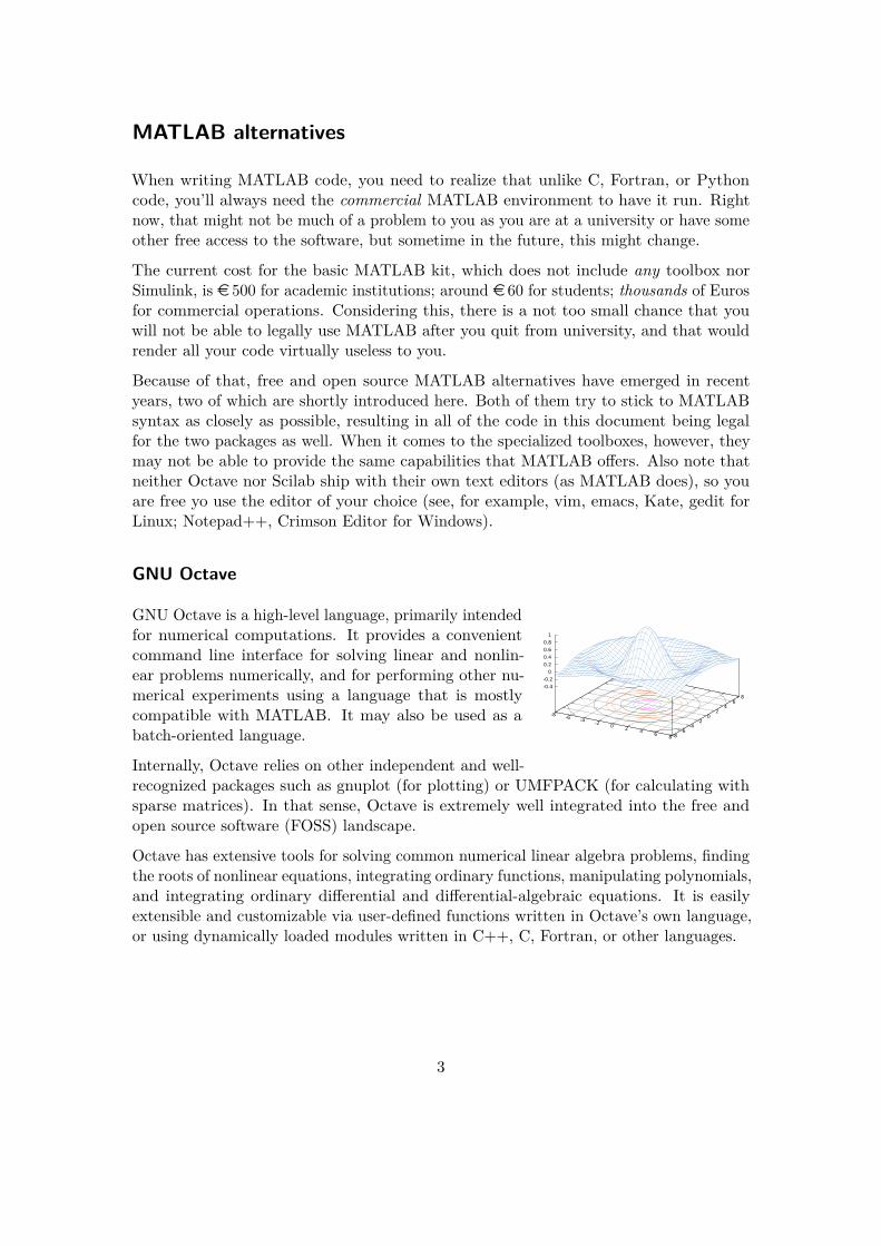
GNU Octave is a high-level language, primarily intendedfor numerical computations. It provides a convenientcommand line interface for solving linear and nonlin-ear problems numerically, and for performing other nu-merical experiments using a language that is mostlycompatible with MATLAB. It may also be used as abatch-oriented language.

Internally, Octave relies on other independent and well-recognized packages such as gnuplot (for plotting) or UMFPACK (for calculating withsparse matrices). In that sense, Octave is extremely well integrated into the free andopen source software (FOSS) landscape.

Octave has extensive tools for solving common numerical linear algebra problems, findingthe roots of nonlinear equations, integrating ordinary functions, manipulating polynomials,and integrating ordinary differential and differential-algebraic equations. It is easilyextensible and customizable via user-defined functions written in Octave’s own language,or using dynamically loaded modules written in C++, C, Fortran, or other languages.

3

GNU Octave is also freely redistributable software. You may redistribute it and/ormodify it under the terms of the GNU General Public License (GPL) as published bythe Free Software Foundation.

The project if originally GNU/Linux, but versions for MacOS, Windows, Sun Solaris,and OS/2 exist.

Scilab

Scilab is a scientific software package for numerical computa-tions providing a powerful open computing environment forengineering and scientific applications.

Scilab is open source software and originates from the FrenchInternational Institute for Research in Computer Science andControl (INRIA).

Since 1994 it has been distributed freely along with the source code via the Internet. Itis currently used in educational and industrial environments around the world.

Scilab is now the responsibility of the Scilab Consortium, launched in May 2003. Thereare currently 18 members in Scilab Consortium (Phase II).

Scilab includes hundreds of mathematical functions with the possibility to add inter-actively programs from various languages (C, C++, Fortran,. . . ). It has sophisticateddata structures (including lists, polynomials, rational functions, linear systems. . . ), aninterpreter and a high level programming language.

Scilab works under Windows 9X/2000/XP/Vista, GNU/Linux, and most UNIX systems.Binary versions for these systems are freely available, along with the source code.

4

1 Coding clean

There is a plethora of reasons why code that just works™ is not good enough. Take apeek at listing 1 and admit:

• Fixing bugs, adding features, and working with the code in all other aspects get alot easier when the code isn’t messy.

• Imagine someone else looking at your code, and trying to figure out what it does.In case you have you didn’t keep it clean, that will certainly be a huge waste oftime.

• You might be planning to code for a particular purpose now, not planning on everusing it again, but experience tells that there is virtually no computational taskthat you come across only once in your programming life. Imagine yourself lookingat your own code, a week, a month, or a year from now: Would you still be able tounderstand why the code works as it does? Clean code will make sure you do.

Examples of messy, unstructured, and generally ugly programs are plenty, but thereare also places where you are almost guaranteed to find well-structured code. Take,for example the MATLAB internals: Many of the functions that you might make useof when programming MATLAB are implemented in MATLAB syntax themselves –by professional MathWorks programmers. To look at such the contents of the mean()function (which calculates the average mean value of an array), type edit mean on theMATLAB command line. You might not be able to understand what’s going on, but theway the file looks like may give you hints on how to write clean code.

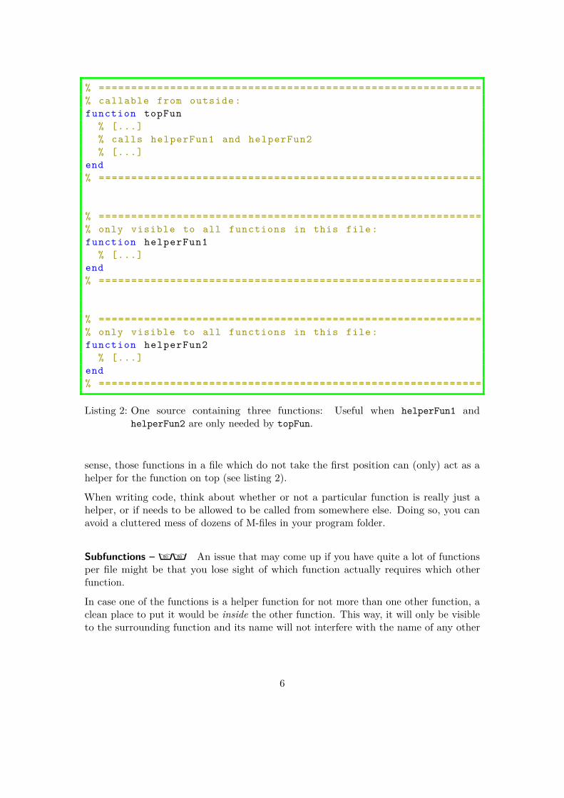
Multiple functions per file – ÕÕÕ

It is a common and false prejudice that MATLAB cannot cope with several functionsper file. The truth is: There may be more than one function in a file, but just the firstone in the file will be visible to functions in other files or to the command line. In that

function lll(ll1 ,l11 ,l1l );if floor(l11/ll1 ) <=1;...lll(ll1 ,l11 +1, l1l ); elseif mod(l11 ,ll1 )==0; lll (...ll1 ,l11 +1 ,0); elseif mod(l11 ,ll1 )== floor(l11 /...ll1 )&&~ l1l;floor(l11/ll1),lll(ll1 ,l11 +1 ,0); elseif ...mod(l11 ,ll1 ) >1&& mod(l11 ,ll1)<floor(l11/ll1 ) ,...lll(ll1 ,l11 +1, l1l +~ mod(floor(l11/ll1),mod(l11 ,ll1 )) );elseif l11 <ll1*ll1;lll(ll1 ,l11 +1, l1l ); end;end

Listing 1: Perfectly legal MATLAB code, with all rules of style ignored. Can you guesswhat this function does?

5

% ===========================================================% callable from outside :function topFun

% [...]% calls helperFun1 and helperFun2% [...]

end% ===========================================================

% ===========================================================% only visible to all functions in this file:function helperFun1

% [...]end% ===========================================================

% ===========================================================% only visible to all functions in this file:function helperFun2

% [...]end% ===========================================================

Listing 2: One source containing three functions: Useful when helperFun1 andhelperFun2 are only needed by topFun.

sense, those functions in a file which do not take the first position can (only) act as ahelper for the function on top (see listing 2).

When writing code, think about whether or not a particular function is really just ahelper, or if needs to be allowed to be called from somewhere else. Doing so, you canavoid a cluttered mess of dozens of M-files in your program folder.

Subfunctions – ÕÕ An issue that may come up if you have quite a lot of functionsper file might be that you lose sight of which function actually requires which otherfunction.

In case one of the functions is a helper function for not more than one other function, aclean place to put it would be inside the other function. This way, it will only be visibleto the surrounding function and its name will not interfere with the name of any other

6

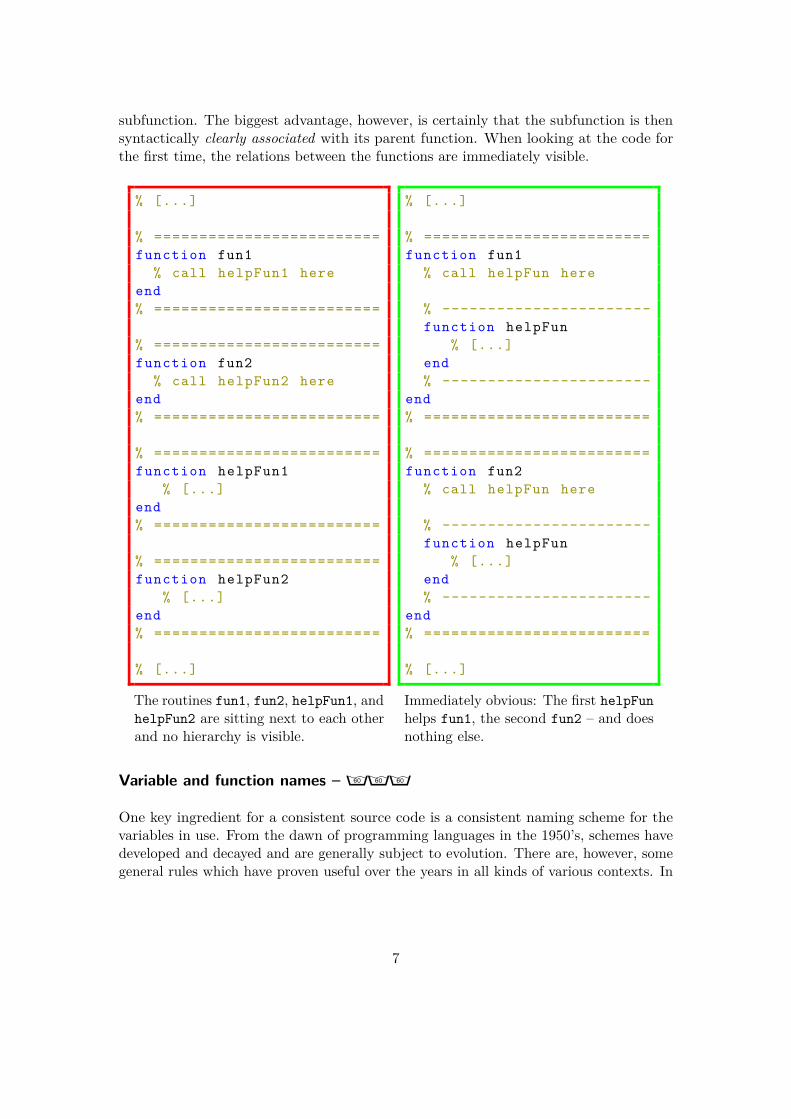
subfunction. The biggest advantage, however, is certainly that the subfunction is thensyntactically clearly associated with its parent function. When looking at the code forthe first time, the relations between the functions are immediately visible.

% [...]

% =========================function fun1

% call helpFun1 hereend% =========================

% =========================function fun2

% call helpFun2 hereend% =========================

% =========================function helpFun1

% [...]end% =========================

% =========================function helpFun2

% [...]end% =========================

% [...]

The routines fun1, fun2, helpFun1, andhelpFun2 are sitting next to each otherand no hierarchy is visible.

% [...]

% =========================function fun1

% call helpFun here

% -----------------------function helpFun

% [...]end% -----------------------

end% =========================

% =========================function fun2

% call helpFun here

% -----------------------function helpFun

% [...]end% -----------------------

end% =========================

% [...]

Immediately obvious: The first helpFunhelps fun1, the second fun2 – and doesnothing else.

Variable and function names – ÕÕÕ

One key ingredient for a consistent source code is a consistent naming scheme for thevariables in use. From the dawn of programming languages in the 1950’s, schemes havedeveloped and decayed and are generally subject to evolution. There are, however, somegeneral rules which have proven useful over the years in all kinds of various contexts. In

7

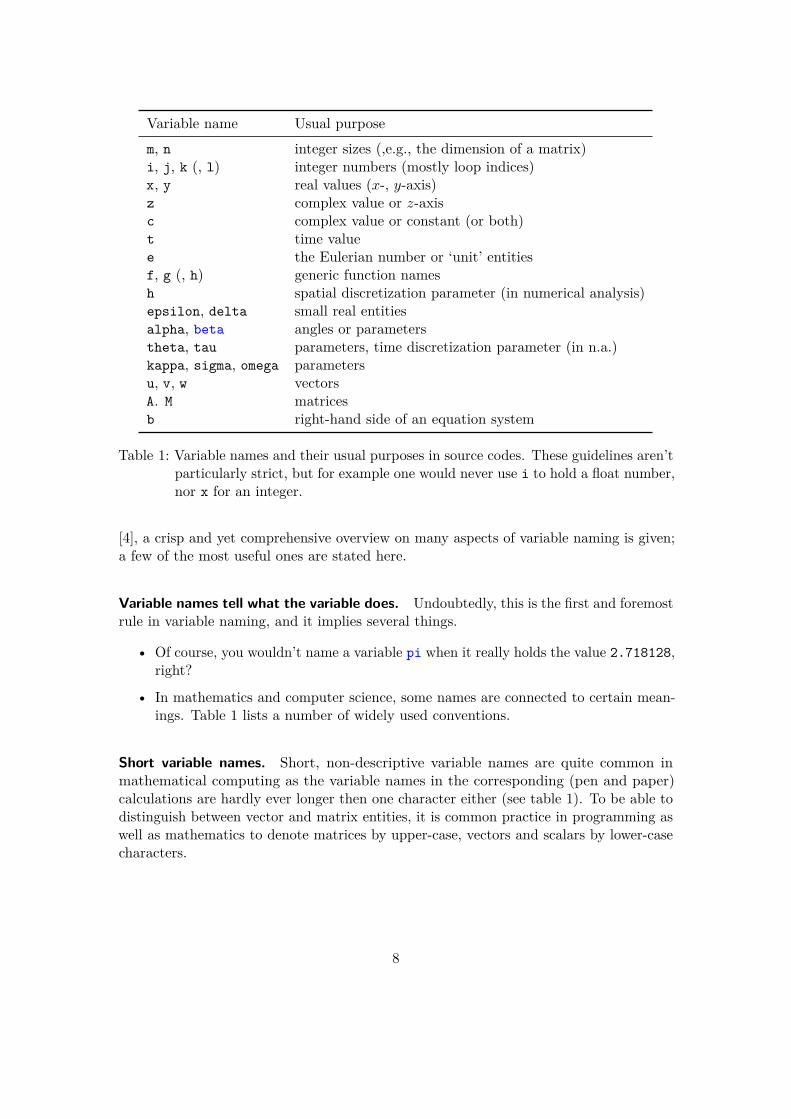
Variable name Usual purpose

m, n integer sizes (,e.g., the dimension of a matrix)i, j, k (, l) integer numbers (mostly loop indices)x, y real values (x-, y-axis)z complex value or z-axisc complex value or constant (or both)t time valuee the Eulerian number or ‘unit’ entitiesf, g (, h) generic function namesh spatial discretization parameter (in numerical analysis)epsilon, delta small real entitiesalpha, beta angles or parameterstheta, tau parameters, time discretization parameter (in n.a.)kappa, sigma, omega parametersu, v, w vectorsA. M matricesb right-hand side of an equation system

Table 1: Variable names and their usual purposes in source codes. These guidelines aren’tparticularly strict, but for example one would never use i to hold a float number,nor x for an integer.

[4], a crisp and yet comprehensive overview on many aspects of variable naming is given;a few of the most useful ones are stated here.

Variable names tell what the variable does. Undoubtedly, this is the first and foremostrule in variable naming, and it implies several things.

• Of course, you wouldn’t name a variable pi when it really holds the value 2.718128,right?

• In mathematics and computer science, some names are connected to certain mean-ings. Table 1 lists a number of widely used conventions.

Short variable names. Short, non-descriptive variable names are quite common inmathematical computing as the variable names in the corresponding (pen and paper)calculations are hardly ever longer then one character either (see table 1). To be able todistinguish between vector and matrix entities, it is common practice in programming aswell as mathematics to denote matrices by upper-case, vectors and scalars by lower-casecharacters.

8

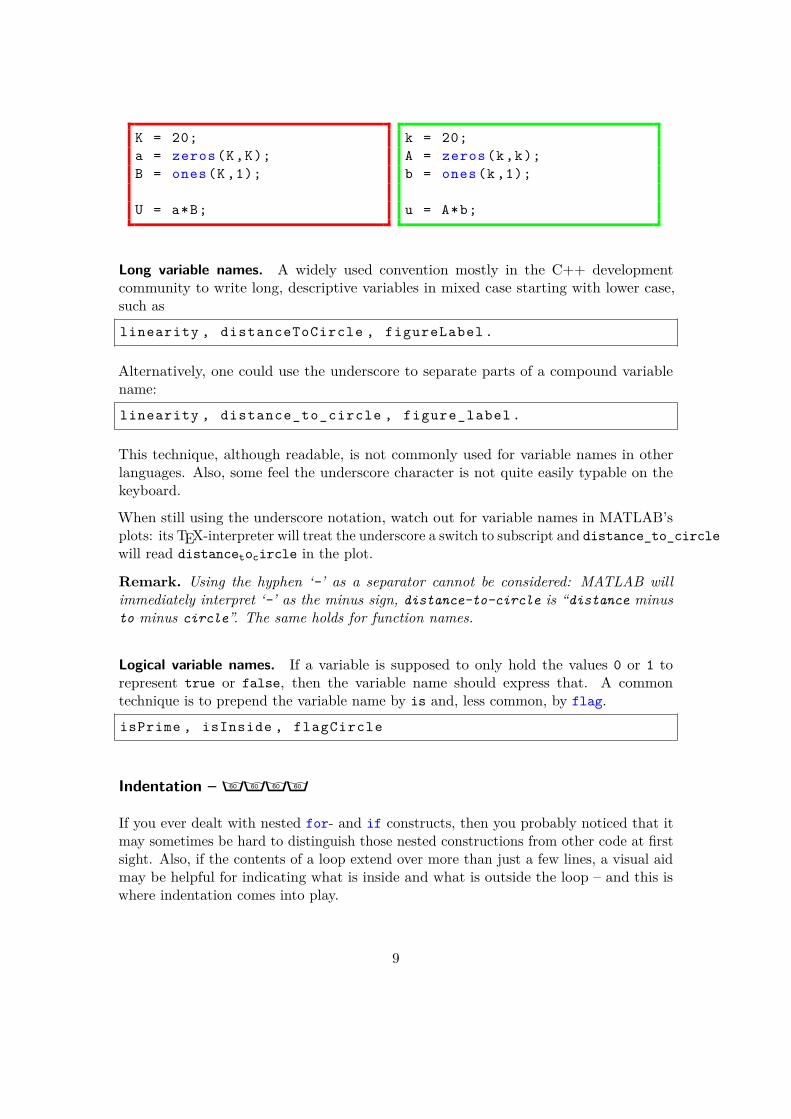
K = 20;a = zeros(K,K);B = ones(K ,1);

U = a*B;

k = 20;A = zeros(k,k);b = ones(k ,1);

u = A*b;

Long variable names. A widely used convention mostly in the C++ developmentcommunity to write long, descriptive variables in mixed case starting with lower case,such as

linearity , distanceToCircle , figureLabel .

Alternatively, one could use the underscore to separate parts of a compound variablename:

linearity , distance_to_circle , figure_label .

This technique, although readable, is not commonly used for variable names in otherlanguages. Also, some feel the underscore character is not quite easily typable on thekeyboard.

When still using the underscore notation, watch out for variable names in MATLAB’splots: its TEX-interpreter will treat the underscore a switch to subscript and distance_to_circlewill read distancetocircle in the plot.

Remark. Using the hyphen ‘-’ as a separator cannot be considered: MATLAB willimmediately interpret ‘-’ as the minus sign, distance-to-circle is “distance minusto minus circle”. The same holds for function names.

Logical variable names. If a variable is supposed to only hold the values 0 or 1 torepresent true or false, then the variable name should express that. A commontechnique is to prepend the variable name by is and, less common, by flag.

isPrime , isInside , flagCircle

Indentation – ÕÕÕÕ

If you ever dealt with nested for- and if constructs, then you probably noticed that itmay sometimes be hard to distinguish those nested constructions from other code at firstsight. Also, if the contents of a loop extend over more than just a few lines, a visual aidmay be helpful for indicating what is inside and what is outside the loop – and this iswhere indentation comes into play.

9

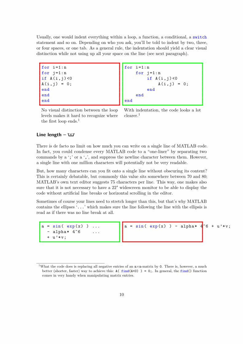
Usually, one would indent everything within a loop, a function, a conditional, a switchstatement and so on. Depending on who you ask, you’ll be told to indent by two, three,or four spaces, or one tab. As a general rule, the indentation should yield a clear visualdistinction while not using up all your space on the line (see next paragraph).

for i=1:nfor j=1:nif A(i,j)<0A(i,j) = 0;endendend

No visual distinction between the looplevels makes it hard to recognize wherethe first loop ends.1

for i=1:nfor j=1:n

if A(i,j)<0A(i,j) = 0;

endend

end

With indentation, the code looks a lotclearer.1

Line length – Õ

There is de facto no limit on how much you can write on a single line of MATLAB code.In fact, you could condense every MATLAB code to a “one-liner” by separating twocommands by a ‘;’ or a ‘,’, and suppress the newline character between them. However,a single line with one million characters will potentially not be very readable.

But, how many characters can you fit onto a single line without obscuring its content?This is certainly debatable, but commonly this value sits somewhere between 70 and 80;MATLAB’s own text editor suggests 75 characters per line. This way, one makes alsosure that it is not necessary to have a 22" widescreen monitor to be able to display thecode without artificial line breaks or horizontal scrolling in the editor.

Sometimes of course your lines need to stretch longer than this, but that’s why MATLABcontains the ellipses ‘...’ which makes sure the line following the line with the ellipsis isread as if there was no line break at all.

a = sin( exp(x) ) ...- alpha * 4^6 ...+ u’*v;

a = sin( exp(x) ) - alpha* 4^6 + u’*v;

1What the code does is replacing all negative entries of an n×n-matrix by 0. There is, however, a muchbetter (shorter, faster) way to achieve this: A( find(A<0) ) = 0;. In general, the find() functioncomes in very handy when manipulating matrix entries.

10

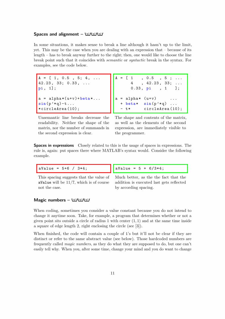
Spaces and alignment – ÕÕÕ

In some situations, it makes sense to break a line although it hasn’t up to the limit,yet. This may be the case when you are dealing with an expression that – because of itslength – has to break anyway further to the right; then, one would like to choose the linebreak point such that it coincides with semantic or syntactic break in the syntax. Forexamples, see the code below.

A = [ 1, 0.5 , 5; 4, ...42.23 , 33; 0.33 , ...pi , 1];

a = alpha *(u+v)+ beta *...sin(p’*q)-t...* circleArea (10);

Unsemantic line breaks decrease thereadability. Neither the shape of thematrix, nor the number of summands inthe second expression is clear.

A = [ 1 , 0.5 , 5 ; ...4 , 42.23 , 33; ...0.33 , pi , 1 ];

a = alpha* (u+v) ...+ beta* sin(p’*q) ...- t* circleArea (10);

The shape and contents of the matrix,as well as the elements of the secondexpression, are immediately visible tothe programmer.

Spaces in expressions Closely related to this is the usage of spaces in expressions. Therule is, again: put spaces there where MATLAB’s syntax would. Consider the followingexample.

aValue = 5+6 / 3*4;

This spacing suggests that the value ofaValue will be 11/7, which is of coursenot the case.

aValue = 5 + 6/3*4;

Much better, as the the fact that theaddition is executed last gets reflectedby according spacing.

Magic numbers – ÕÕÕ

When coding, sometimes you consider a value constant because you do not intend tochange it anytime soon. Take, for example, a program that determines whether or not agiven point sits outside a circle of radius 1 with center (1, 1) and at the same time insidea square of edge length 2, right enclosing the circle (see [3]).

When finished, the code will contain a couple of 1’s but it’ll not be clear if they aredistinct or refer to the same abstract value (see below). Those hardcoded numbers arefrequently called magic numbers, as they do what they are supposed to do, but one can’teasily tell why. When you, after some time, change your mind and you do want to change

11

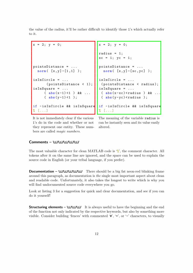
the value of the radius, it’ll be rather difficult to identify those 1’s which actually referto it.

x = 2; y = 0;

pointsDistance = ...norm( [x,y] -[1 ,1] );

isInCircle = ...( pointsDistance < 1);

isInSquare = ...( abs(x -1) <1 ) && ...( abs(y -1) <1 );

if ~ isInCircle && isInSquare% [...]

It is not immediately clear if the various1’s do in the code and whether or notthey represent one entity. These num-bers are called magic numbers.

x = 2; y = 0;

radius = 1;xc = 1; yc = 1;

pointsDistance = ...norm( [x,y]-[xc ,yc] );

isInCircle = ...( pointsDistance < radius );

isInSquare = ...( abs(x-xc)< radius ) && ...( abs(y-yc)< radius );

if ~ isInCircle && isInSquare% [...]

The meaning of the variable radius iscan be instantly seen and its value easilyaltered.

Comments – ÕÕÕÕÕ

The most valuable character for clean MATLAB code is ‘%’, the comment character. Alltokens after it on the same line are ignored, and the space can be used to explain thesource code in English (or your tribal language, if you prefer).

Documentation –ÕÕÕÕÕ There should be a big fat neon-red blinking framearound this paragraph, as documentation is the single most important aspect about cleanand readable code. Unfortunately, it also takes the longest to write which is why youwill find undocumented source code everywhere you go.

Look at listing 3 for a suggestion for quick and clear documentation, and see if you cando it yourself!

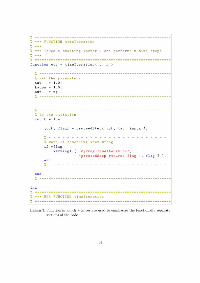
Structuring elements –ÕÕÕ It is always useful to have the beginning and the endof the function not only indicated by the respective keywords, but also by something morevisible. Consider building ‘fences’ with commented ‘#’, ‘=’, or ‘-’ characters, to visually

12

separate distinct parts of the code. This comes in very handy when there are multiplefunctions in one source file, for example, or when there is a for-loop that stretches overthat many lines that you can’t easily find the corresponding end anymore.

For a (slightly exaggerated) example, see listing 3.

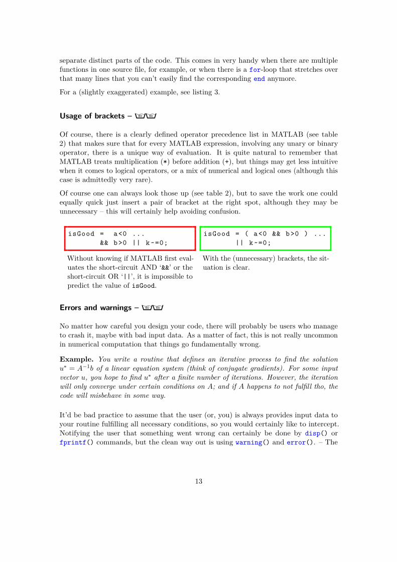
Usage of brackets – ÕÕ

Of course, there is a clearly defined operator precedence list in MATLAB (see table2) that makes sure that for every MATLAB expression, involving any unary or binaryoperator, there is a unique way of evaluation. It is quite natural to remember thatMATLAB treats multiplication (*) before addition (+), but things may get less intuitivewhen it comes to logical operators, or a mix of numerical and logical ones (although thiscase is admittedly very rare).

Of course one can always look those up (see table 2), but to save the work one couldequally quick just insert a pair of bracket at the right spot, although they may beunnecessary – this will certainly help avoiding confusion.

isGood = a<0 ...&& b>0 || k~=0;

Without knowing if MATLAB first eval-uates the short-circuit AND ‘&&’ or theshort-circuit OR ‘||’, it is impossible topredict the value of isGood.

isGood = ( a<0 && b>0 ) ...|| k~=0;

With the (unnecessary) brackets, the sit-uation is clear.

Errors and warnings – ÕÕ

No matter how careful you design your code, there will probably be users who manageto crash it, maybe with bad input data. As a matter of fact, this is not really uncommonin numerical computation that things go fundamentally wrong.

Example. You write a routine that defines an iterative process to find the solutionu∗ = A−1b of a linear equation system (think of conjugate gradients). For some inputvector u, you hope to find u∗ after a finite number of iterations. However, the iterationwill only converge under certain conditions on A; and if A happens to not fulfill tho, thecode will misbehave in some way.

It’d be bad practice to assume that the user (or, you) is always provides input data toyour routine fulfilling all necessary conditions, so you would certainly like to intercept.Notifying the user that something went wrong can certainly be done by disp() orfprintf() commands, but the clean way out is using warning() and error(). – The

13

% ===========================================================% *** FUNCTION timeIteration% ***% *** Takes a starting vector u and performs n time steps.% ***% ===========================================================function out = timeIteration ( u, n )

% ---------------------------------------------------------% set the parameterstau = 1.0;kappa = 1.0;out = u;% ---------------------------------------------------------

% ---------------------------------------------------------% do the iterationfor k = 1:n

[out , flag] = proceedStep ( out , tau , kappa );

% - - - - - - - - - - - - - - - - - - - - - - - - - -% warn if something went wrongif ~flag

warning ( [ ’myProg : timeIteration ’, ...’proceedStep returns flag ’, flag ] );

end% - - - - - - - - - - - - - - - - - - - - - - - - - -

end% ---------------------------------------------------------

end% ===========================================================% *** END FUNCTION timeIteration% ===========================================================

Listing 3: Function in which --fences are used to emphasize the functionally separatesections of the code.

14

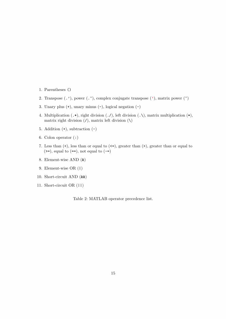
1. Parentheses ()

2. Transpose (.’), power (.^), complex conjugate transpose (’), matrix power (^)

3. Unary plus (+), unary minus (-), logical negation (~)

4. Multiplication (.*), right division (./), left division (.\), matrix multiplication (*),matrix right division (/), matrix left division (\)

5. Addition (+), subtraction (-)

6. Colon operator (:)

7. Less than (<), less than or equal to (<=), greater than (>), greater than or equal to(>=), equal to (==), not equal to (~=)

8. Element-wise AND (&)

9. Element-wise OR (|)

10. Short-circuit AND (&&)

11. Short-circuit OR (||)

Table 2: MATLAB operator precedence list.

15

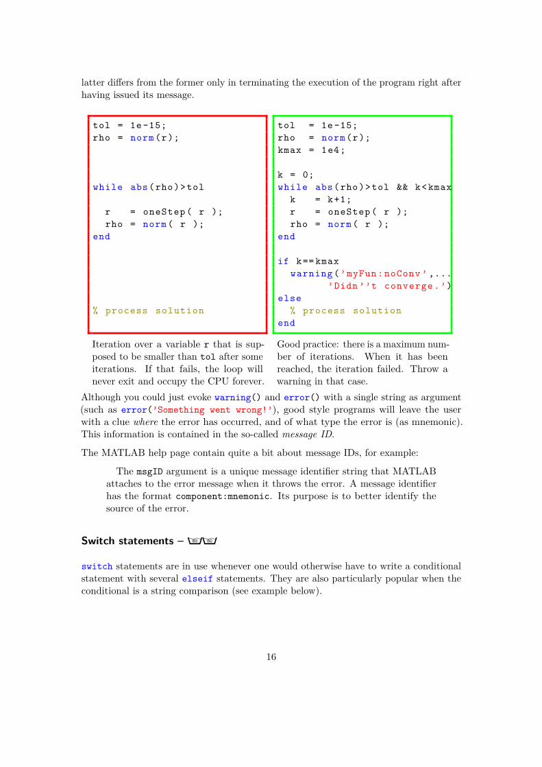
latter differs from the former only in terminating the execution of the program right afterhaving issued its message.

tol = 1e -15;rho = norm(r);

while abs(rho)>tol

r = oneStep ( r );rho = norm( r );

end

% process solution

Iteration over a variable r that is sup-posed to be smaller than tol after someiterations. If that fails, the loop willnever exit and occupy the CPU forever.

tol = 1e -15;rho = norm(r);kmax = 1e4;

k = 0;while abs(rho)>tol && k<kmax

k = k+1;r = oneStep ( r );rho = norm( r );

end

if k== kmaxwarning (’myFun: noConv ’ ,...

’Didn ’’t converge .’)else

% process solutionend

Good practice: there is a maximum num-ber of iterations. When it has beenreached, the iteration failed. Throw awarning in that case.

Although you could just evoke warning() and error() with a single string as argument(such as error(’Something went wrong!’), good style programs will leave the userwith a clue where the error has occurred, and of what type the error is (as mnemonic).This information is contained in the so-called message ID.

The MATLAB help page contain quite a bit about message IDs, for example:

The msgID argument is a unique message identifier string that MATLABattaches to the error message when it throws the error. A message identifierhas the format component:mnemonic. Its purpose is to better identify thesource of the error.

Switch statements – ÕÕ

switch statements are in use whenever one would otherwise have to write a conditionalstatement with several elseif statements. They are also particularly popular when theconditional is a string comparison (see example below).

16

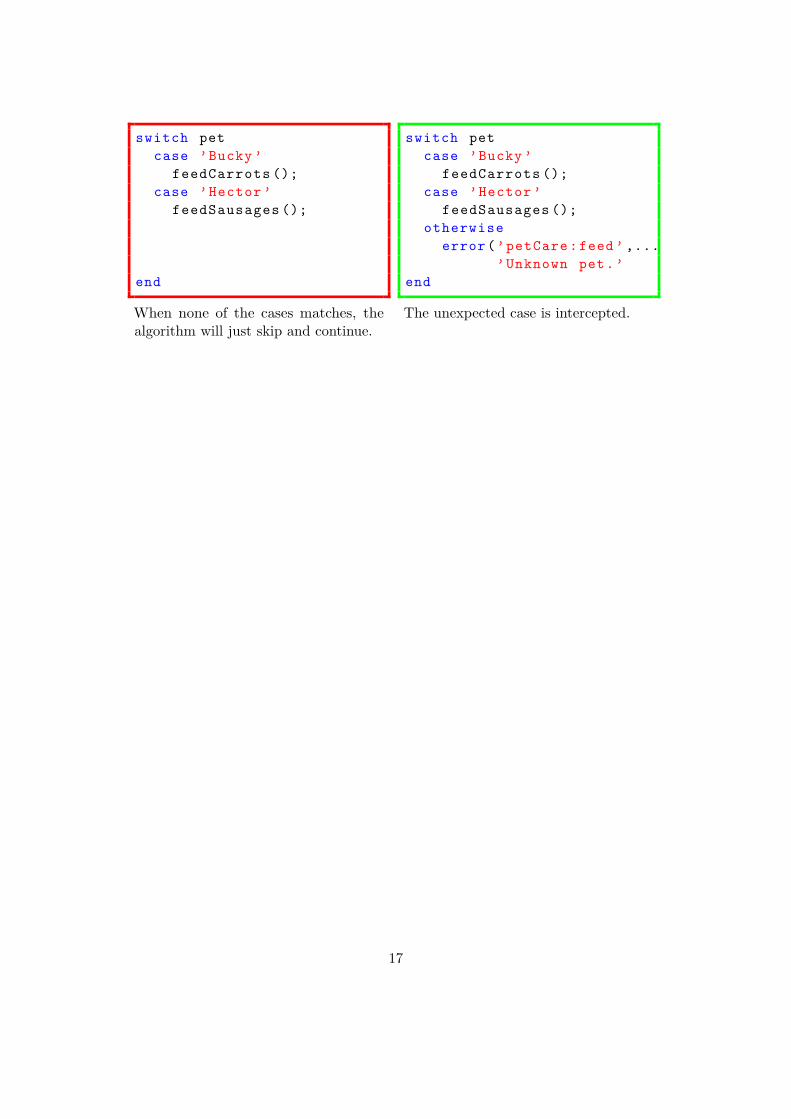
switch petcase ’Bucky ’

feedCarrots ();case ’Hector ’

feedSausages ();

end

When none of the cases matches, thealgorithm will just skip and continue.

switch petcase ’Bucky ’

feedCarrots ();case ’Hector ’

feedSausages ();otherwise

error(’petCare :feed ’ ,...’Unknown pet.’

end

The unexpected case is intercepted.

17

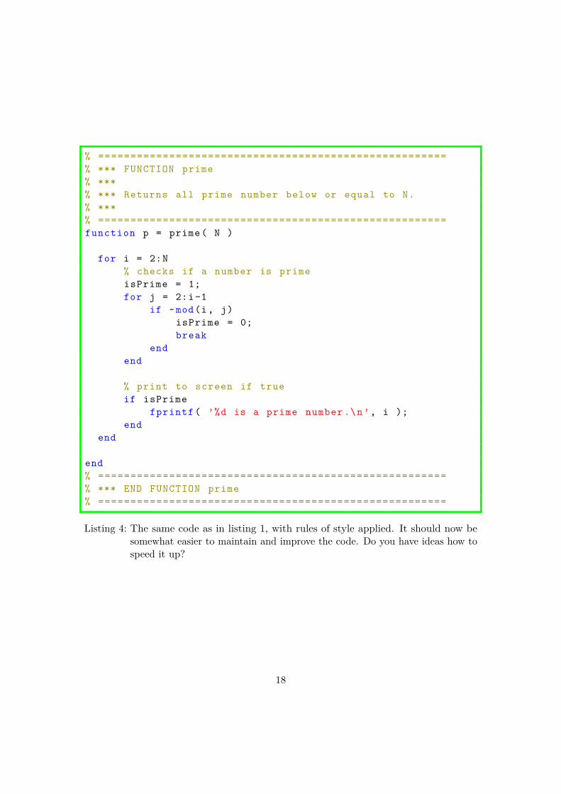
% ======================================================% *** FUNCTION prime% ***% *** Returns all prime number below or equal to N.% ***% ======================================================function p = prime( N )

for i = 2:N% checks if a number is primeisPrime = 1;for j = 2:i-1

if ~mod(i, j)isPrime = 0;break

endend

% print to screen if trueif isPrime

fprintf ( ’%d is a prime number .\n’, i );end

end

end% ======================================================% *** END FUNCTION prime% ======================================================

Listing 4: The same code as in listing 1, with rules of style applied. It should now besomewhat easier to maintain and improve the code. Do you have ideas how tospeed it up?

18

2 Coding fast

As a MATLAB beginner, it is quite easy to use code that just works™but comparing tocompiled programs of higher programming languages is very slow. The benefit of therelatively straightforward way of programming in MATLAB (where no such things asexplicit memory allocation, pointers, or data types “come in your way”) needs to be paidwith the knowledge of how to avoid fundamental mistakes. Fortunately, there are only afew big ones, so when you browse through this section and stick to the given hints, youcan certainly be quite confident about your code.

Using the profiler

The first step in optimizing the speed of your program is finding out where it is actuallygoing slow. In traditional programming, bottlenecks are not quite easily found, and thehumble coder would maybe insert timer commands around those chunks of code wherehe or she suspects the delay to actually measure its performance. You can do the samething in MATLAB (using tic and toc as timers) but there is a much more convenientway: the profiler.

The profiler is actually a wrapper around your whole program that measures the executiontime of each and every single line of code and depicts the result graphically. This way,you can very quickly track down the lines that keep you from going fast. See figure 1 foran example output.

Remark. Besides the graphical interface, there is also a command line version of theprofiler that can be used to integrate it into your scripts. The commands to invoke areprofile on for starting the profiler and profile off for stopping it, followed by variouscommands to evaluate the gathers statistics. See the MATLAB help page on profile.

The MATtrix LABoratory

Contrary to common belief, the MAT in MATLAB doesn’t stand for mathematics,but matrix. The reason for that is that proper MATLAB code uses matrix and vectorstructures as often as possible, prominently at places where higher programming languagessuch as C of Fortran would rather use loops.

The reason for that lies in MATLAB’s being an interpreted language. That means: Thereis no need for explicitly compiling the code, you just write it and have in run. TheMATLAB interpreter then scans your code line by line and executes the commands. Asyou might already suspect, this approach will never be able to compete with compiledsource code.

19

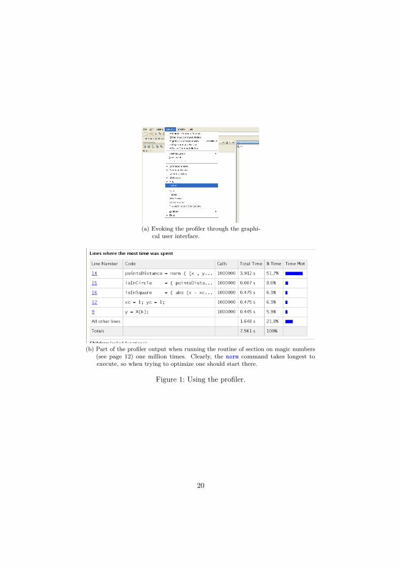
(a) Evoking the profiler through the graphi-cal user interface.

(b) Part of the profiler output when running the routine of section on magic numbers(see page 12) one million times. Clearly, the norm command takes longest toexecute, so when trying to optimize one should start there.

Figure 1: Using the profiler.

20

However, MATLAB’s internals contain certain precompiled functions which execute basicmatrix-vector operations. Whenever the MATLAB interpreter bumps into a matrix-vector expression, the contents of the matrices are forwarded to the underlying optimizedand compiled code which, after execution, returns the result. This approach makes surethat matrix operations in MATLAB are on par with matrix operations with compiledlanguages.

Remark. Not only for matrix-vector operations, precompiled binaries are provided. Moststandard tasks in numerical linear algebra are handled with a customized version of theATLAS (BLAS) library. This concerns for example commands such as eig() (for findingthe eigenvalues of a matrix), \ (for solving a linear equation system with Gaußian2

elimination), and so on.

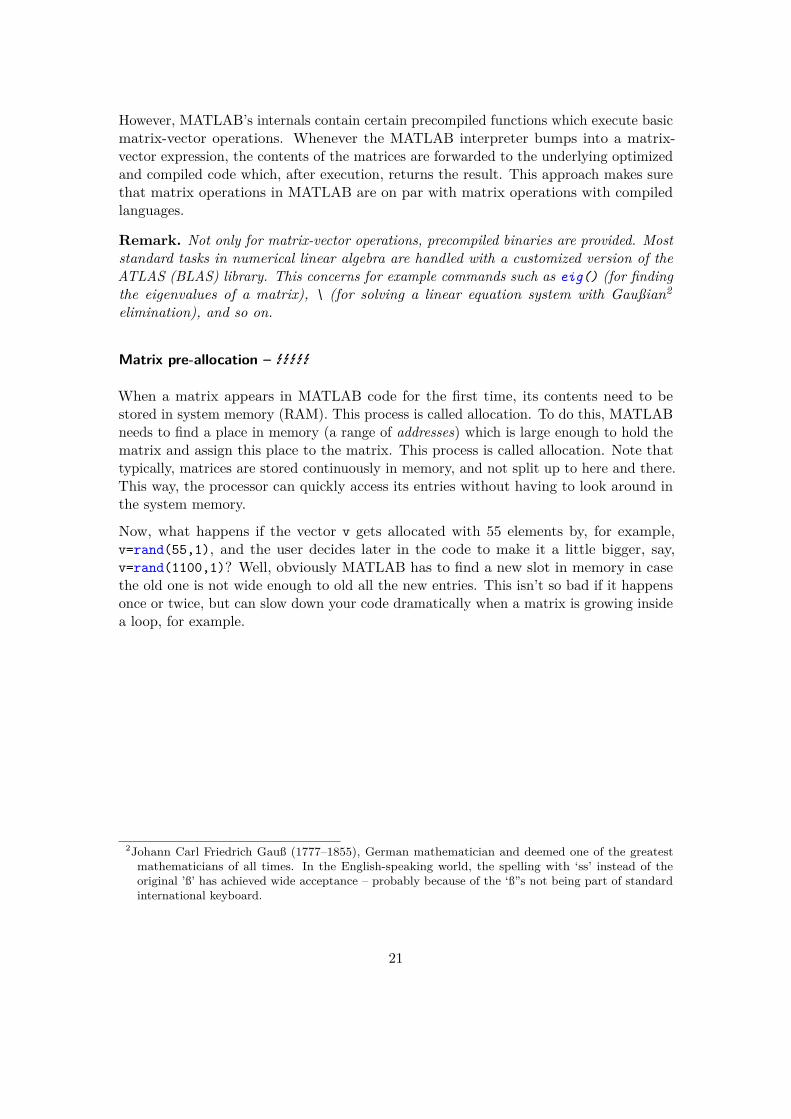
Matrix pre-allocation – EEEEE

When a matrix appears in MATLAB code for the first time, its contents need to bestored in system memory (RAM). This process is called allocation. To do this, MATLABneeds to find a place in memory (a range of addresses) which is large enough to hold thematrix and assign this place to the matrix. This process is called allocation. Note thattypically, matrices are stored continuously in memory, and not split up to here and there.This way, the processor can quickly access its entries without having to look around inthe system memory.

Now, what happens if the vector v gets allocated with 55 elements by, for example,v=rand(55,1), and the user decides later in the code to make it a little bigger, say,v=rand(1100,1)? Well, obviously MATLAB has to find a new slot in memory in casethe old one is not wide enough to old all the new entries. This isn’t so bad if it happensonce or twice, but can slow down your code dramatically when a matrix is growing insidea loop, for example.

2Johann Carl Friedrich Gauß (1777–1855), German mathematician and deemed one of the greatestmathematicians of all times. In the English-speaking world, the spelling with ‘ss’ instead of theoriginal ’ß’ has achieved wide acceptance – probably because of the ‘ß”s not being part of standardinternational keyboard.

21

n = 1e5;

for i = 1:nu(i) = sqrt(i);

end

The vector u is growing n times and itprobably must be re-allocated as often.The approximate execution time of thiscode snippet is 21.20 s.

n = 1e5;u = zeros(n ,1);for i = 1:n

u(i) = sqrt(i);end

As maximum size of the vector isknown beforehand, one can easily tellMATLAB to place u into memory withthe appropriate size. The code heremerely takes 3.8 ms to execute!

Remark. The previous code example is actually a little misleading as there is a muchquicker way to fill u with the square roots of consecutive numbers. Can you find theone-liner? A look into the next section could help. . .

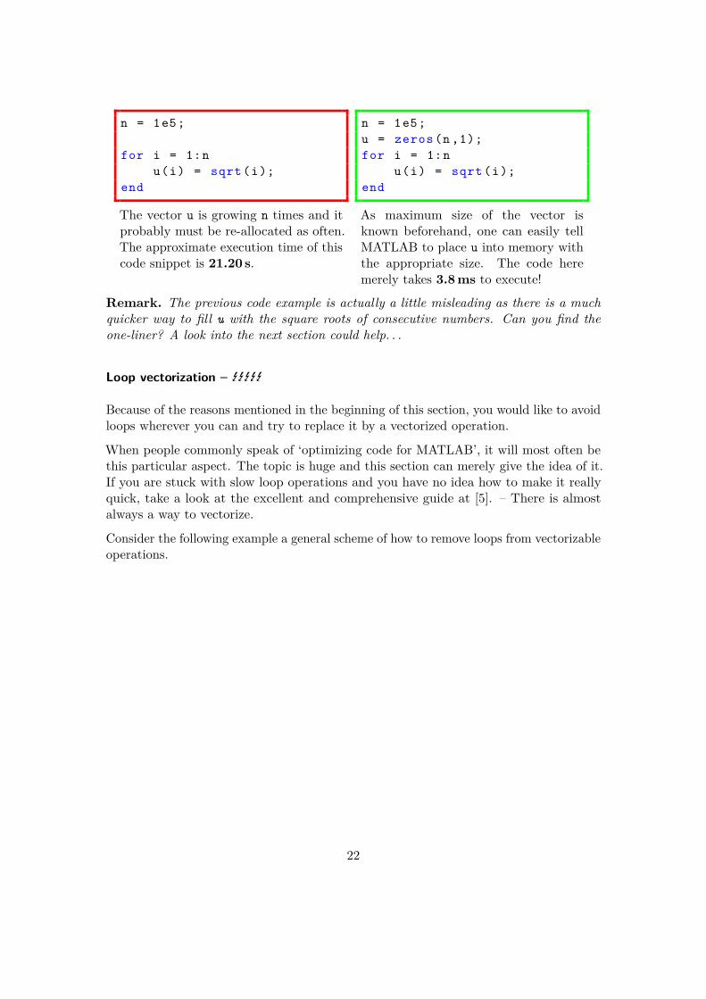
Loop vectorization – EEEEE

Because of the reasons mentioned in the beginning of this section, you would like to avoidloops wherever you can and try to replace it by a vectorized operation.

When people commonly speak of ‘optimizing code for MATLAB’, it will most often bethis particular aspect. The topic is huge and this section can merely give the idea of it.If you are stuck with slow loop operations and you have no idea how to make it reallyquick, take a look at the excellent and comprehensive guide at [5]. – There is almostalways a way to vectorize.

Consider the following example a general scheme of how to remove loops from vectorizableoperations.

22

n = 1e7;a = 1;b = 2;

x = zeros( n, 1 );y = zeros( n, 1 );for i=1:n

x(i) = a + (b-a)/(n -1) ...* (i -1);

y(i) = x(i) - sin(x(i))^2;end

Computation of f(x) = x − sin2(x) onn points between a and b. In this ver-sion, each and every single point is beingtreated explicitly. Execution time: ap-prox. 0.91 s.

n = 1e7;a = 1;b = 2;

h = 1/(n -1);

x = (a:h:b);

y = x - sin(x).^2;

Does the same thing using vector nota-tion. Execution time: approx. 0.12 s.

The sin() function in MATLAB hence takes a vector as argument and acts as of itoperated on each element of it. Almost all MATLAB functions have this capability, somake use of it if you can!

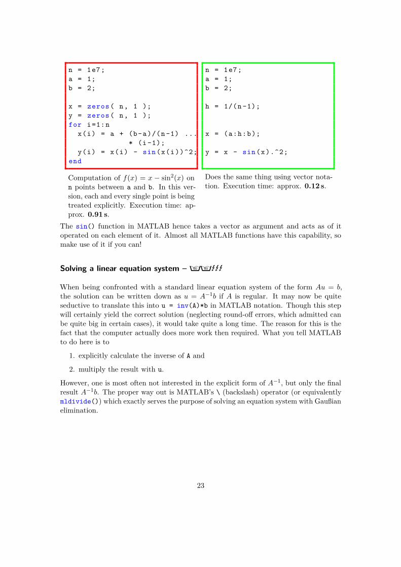
Solving a linear equation system – ÕÕEEE

When being confronted with a standard linear equation system of the form Au = b,the solution can be written down as u = A−1b if A is regular. It may now be quiteseductive to translate this into u = inv(A)*b in MATLAB notation. Though this stepwill certainly yield the correct solution (neglecting round-off errors, which admitted canbe quite big in certain cases), it would take quite a long time. The reason for this is thefact that the computer actually does more work then required. What you tell MATLABto do here is to

1. explicitly calculate the inverse of A and

2. multiply the result with u.

However, one is most often not interested in the explicit form of A−1, but only the finalresult A−1b. The proper way out is MATLAB’s \ (backslash) operator (or equivalentlymldivide()) which exactly serves the purpose of solving an equation system with Gaußianelimination.

23

n = 2e3;A = rand(n,n);b = rand(n ,1);

u = inv(A)*b;

Solving the equation system with an ex-plicit inverse. Execution time: approx.2.02 s.

n = 2e3;A = rand(n,n);b = rand(n ,1);

u = A\b;

Solving the equation system with the\ operator. Execution time: approx.0.80 s.

Dense and sparse matrices – EEEEE

Most discretizations of particular problems yield N ×N -matrices which only have a smallnumber of non-zero elements (proportional to N). These are called sparse matrices, andas they appear so very often, there is plenty of literature describing how to make use ofthat structure.

In particular, one can

• cut down the amount of memory used to store the matrix. Of course, instead ofstoring all the 0’s, one would rather store the value and indices of the non-zeroelements in the matrix. There are different ways of doing so. MATLAB internallyuses the condensed-column format, and exposes the matrix to the user in indexedformat.

• optimize algorithms for the use with sparse matrices. As a matter of fact, mostbasic numerical operations (such as Gaußian elimination, eigenvalue methods andso forth) can be reformulated for sparse matrices and save an enormous amount ofcomputational time.

Of course, operations which only involve sparse matrices will also return a sparse matrix(such as matrix–matrix multiplication *, transpose, kron, and so forth).

24

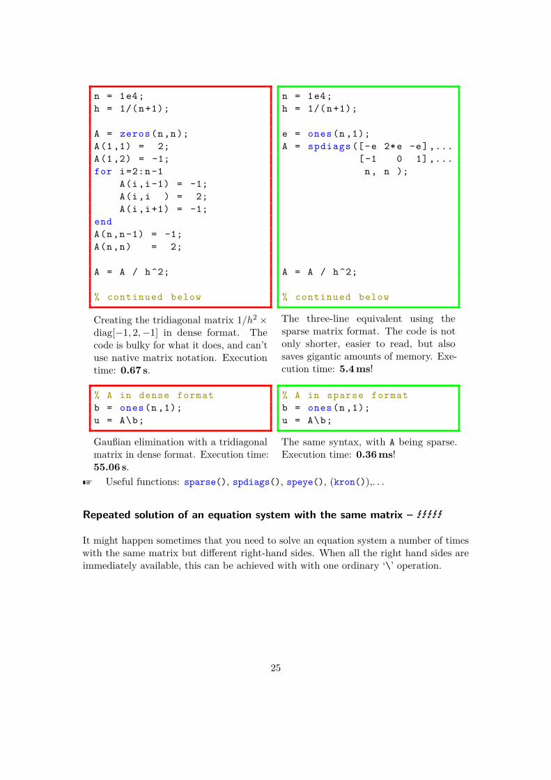
n = 1e4;h = 1/(n+1);

A = zeros(n,n);A(1 ,1) = 2;A(1 ,2) = -1;for i=2:n-1

A(i,i -1) = -1;A(i,i ) = 2;A(i,i+1) = -1;

endA(n,n -1) = -1;A(n,n) = 2;

A = A / h^2;

% continued below

Creating the tridiagonal matrix 1/h2 ×diag[−1, 2,−1] in dense format. Thecode is bulky for what it does, and can’tuse native matrix notation. Executiontime: 0.67 s.

n = 1e4;h = 1/(n+1);

e = ones(n ,1);A = spdiags ([-e 2*e -e] ,...

[-1 0 1] ,...n, n );

A = A / h^2;

% continued below

The three-line equivalent using thesparse matrix format. The code is notonly shorter, easier to read, but alsosaves gigantic amounts of memory. Exe-cution time: 5.4 ms!

% A in dense formatb = ones(n ,1);u = A\b;

Gaußian elimination with a tridiagonalmatrix in dense format. Execution time:55.06 s.

% A in sparse formatb = ones(n ,1);u = A\b;

The same syntax, with A being sparse.Execution time: 0.36 ms!

Z Useful functions: sparse(), spdiags(), speye(), (kron()),. . .

Repeated solution of an equation system with the same matrix – EEEEE

It might happen sometimes that you need to solve an equation system a number of timeswith the same matrix but different right-hand sides. When all the right hand sides areimmediately available, this can be achieved with with one ordinary ‘\’ operation.

25

n = 1e3;k = 50;A = rand(n,n);B = rand(n,k);

u = zeros(n,k);

for i=1:ku(:.k) = A \ B(:,k);

end

Consecutively solving with a coupleof right-hand sides. Execution time:5.64 s.

n = 1e3;k = 50;A = rand(n,n);B = rand(n,k);

u = A \ B;

Solving with a number of right handsides in one go. Execution time: 0.13 s.

If, on the other hand, you need to solve the system once to get the next right-hand side(which is often the case with time-dependent differential equations, for example), thisapproach won’t work; you’ll indeed have to solve the system in a loop. However, onewould still want to use the information from the previous steps; this can be done by firstfactoring A into a product of a lower triangular matrix L and an upper triangular matrixU , and then instead of computing A−1u(k) in each step, computing U−1L−1u(k) (whichis a lot cheaper.

n = 2e3;k = 50;A = rand(n,n);

u = ones(n ,1);

for i = 1:ku = A\u;

end

Computing u = A−ku0 by solving theequation systems in the ordinary way.Execution time: 38.94 s.

n = 2e3;k = 50;A = rand(n,n);

u = ones(n ,1);

[L,U] = lu( A );for i = 1:k

u = U\( L\u );end

Computing u = A−ku0 by LU-factoringthe matrix, then solving with the LUfactors. Execution time: 5.35 s. Ofcourse, when increasing the number k ofiterations, the speed gain compared tothe ‘A\’ will be more and more dramatic.

Remark. For many matrices A in the above example, the final result will be heavilycorrupted with round-off errors such that after k = 50 steps, the norm of the residual∥∥∥u0 −Aku

∥∥∥, which ideally equals 0, can be pretty large.

26

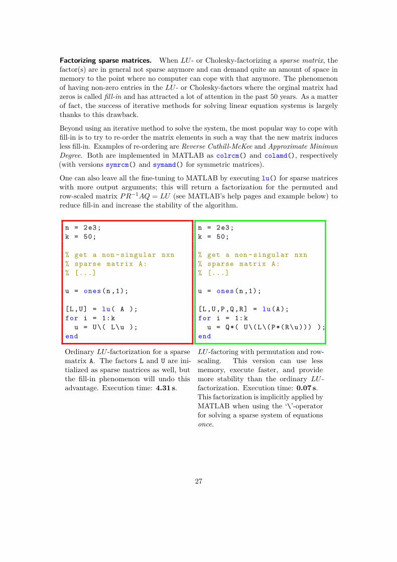
Factorizing sparse matrices. When LU - or Cholesky-factorizing a sparse matrix, thefactor(s) are in general not sparse anymore and can demand quite an amount of space inmemory to the point where no computer can cope with that anymore. The phenomenonof having non-zero entries in the LU - or Cholesky-factors where the orginal matrix hadzeros is called fill-in and has attracted a lot of attention in the past 50 years. As a matterof fact, the success of iterative methods for solving linear equation systems is largelythanks to this drawback.

Beyond using an iterative method to solve the system, the most popular way to cope withfill-in is to try to re-order the matrix elements in such a way that the new matrix inducesless fill-in. Examples of re-ordering are Reverse Cuthill-McKee and Approximate MinimunDegree. Both are implemented in MATLAB as colrcm() and colamd(), respectively(with versions symrcm() and symamd() for symmetric matrices).

One can also leave all the fine-tuning to MATLAB by executing lu() for sparse matriceswith more output arguments; this will return a factorization for the permuted androw-scaled matrix PR−1AQ = LU (see MATLAB’s help pages and example below) toreduce fill-in and increase the stability of the algorithm.

n = 2e3;k = 50;

% get a non - singular nxn% sparse matrix A:% [...]

u = ones(n ,1);

[L,U] = lu( A );for i = 1:k

u = U\( L\u );end

Ordinary LU -factorization for a sparsematrix A. The factors L and U are ini-tialized as sparse matrices as well, butthe fill-in phenomenon will undo thisadvantage. Execution time: 4.31 s.

n = 2e3;k = 50;

% get a non - singular nxn% sparse matrix A:% [...]

u = ones(n ,1);

[L,U,P,Q,R] = lu(A);for i = 1:k

u = Q*( U\(L\(P*(R\u))) );end

LU -factoring with permutation and row-scaling. This version can use lessmemory, execute faster, and providemore stability than the ordinary LU -factorization. Execution time: 0.07 s.This factorization is implicitly applied byMATLAB when using the ‘\’-operatorfor solving a sparse system of equationsonce.

27

3 Other tips & tricks

Functions as arguments – ÕÕÕ

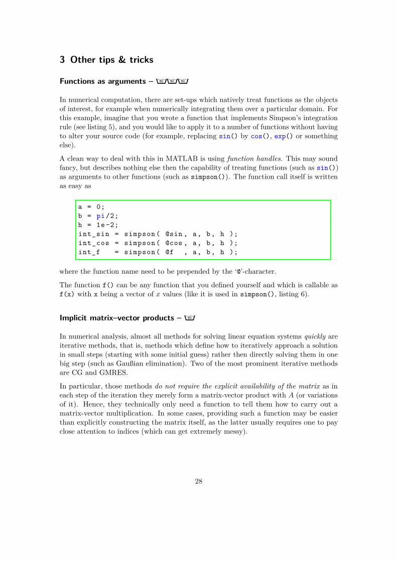
In numerical computation, there are set-ups which natively treat functions as the objectsof interest, for example when numerically integrating them over a particular domain. Forthis example, imagine that you wrote a function that implements Simpson’s integrationrule (see listing 5), and you would like to apply it to a number of functions without havingto alter your source code (for example, replacing sin() by cos(), exp() or somethingelse).

A clean way to deal with this in MATLAB is using function handles. This may soundfancy, but describes nothing else then the capability of treating functions (such as sin())as arguments to other functions (such as simpson()). The function call itself is writtenas easy as

a = 0;b = pi /2;h = 1e -2;int_sin = simpson ( @sin , a, b, h );int_cos = simpson ( @cos , a, b, h );int_f = simpson ( @f , a, b, h );

where the function name need to be prepended by the ‘@’-character.

The function f() can be any function that you defined yourself and which is callable asf(x) with x being a vector of x values (like it is used in simpson(), listing 6).

Implicit matrix–vector products – Õ

In numerical analysis, almost all methods for solving linear equation systems quickly areiterative methods, that is, methods which define how to iteratively approach a solutionin small steps (starting with some initial guess) rather then directly solving them in onebig step (such as Gaußian elimination). Two of the most prominent iterative methodsare CG and GMRES.

In particular, those methods do not require the explicit availability of the matrix as ineach step of the iteration they merely form a matrix-vector product with A (or variationsof it). Hence, they technically only need a function to tell them how to carry out amatrix-vector multiplication. In some cases, providing such a function may be easierthan explicitly constructing the matrix itself, as the latter usually requires one to payclose attention to indices (which can get extremely messy).

28

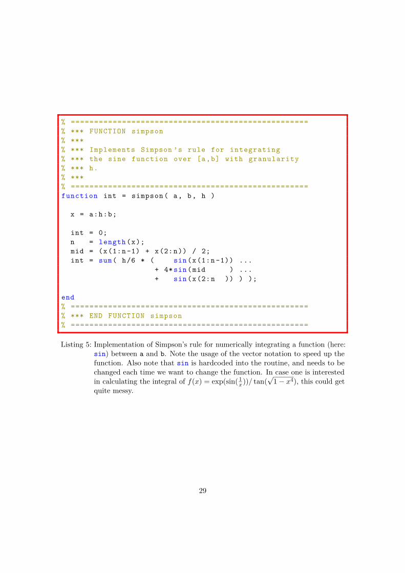
% ===================================================% *** FUNCTION simpson% ***% *** Implements Simpson ’s rule for integrating% *** the sine function over [a,b] with granularity% *** h.% ***% ===================================================function int = simpson ( a, b, h )

x = a:h:b;

int = 0;n = length (x);mid = (x(1:n -1) + x(2:n)) / 2;int = sum( h/6 * ( sin(x(1:n -1)) ...

+ 4* sin(mid ) ...+ sin(x(2:n )) ) );

end% ===================================================% *** END FUNCTION simpson% ===================================================

Listing 5: Implementation of Simpson’s rule for numerically integrating a function (here:sin) between a and b. Note the usage of the vector notation to speed up thefunction. Also note that sin is hardcoded into the routine, and needs to bechanged each time we want to change the function. In case one is interestedin calculating the integral of f(x) = exp(sin( 1

x))/ tan(√

1− x4), this could getquite messy.

29

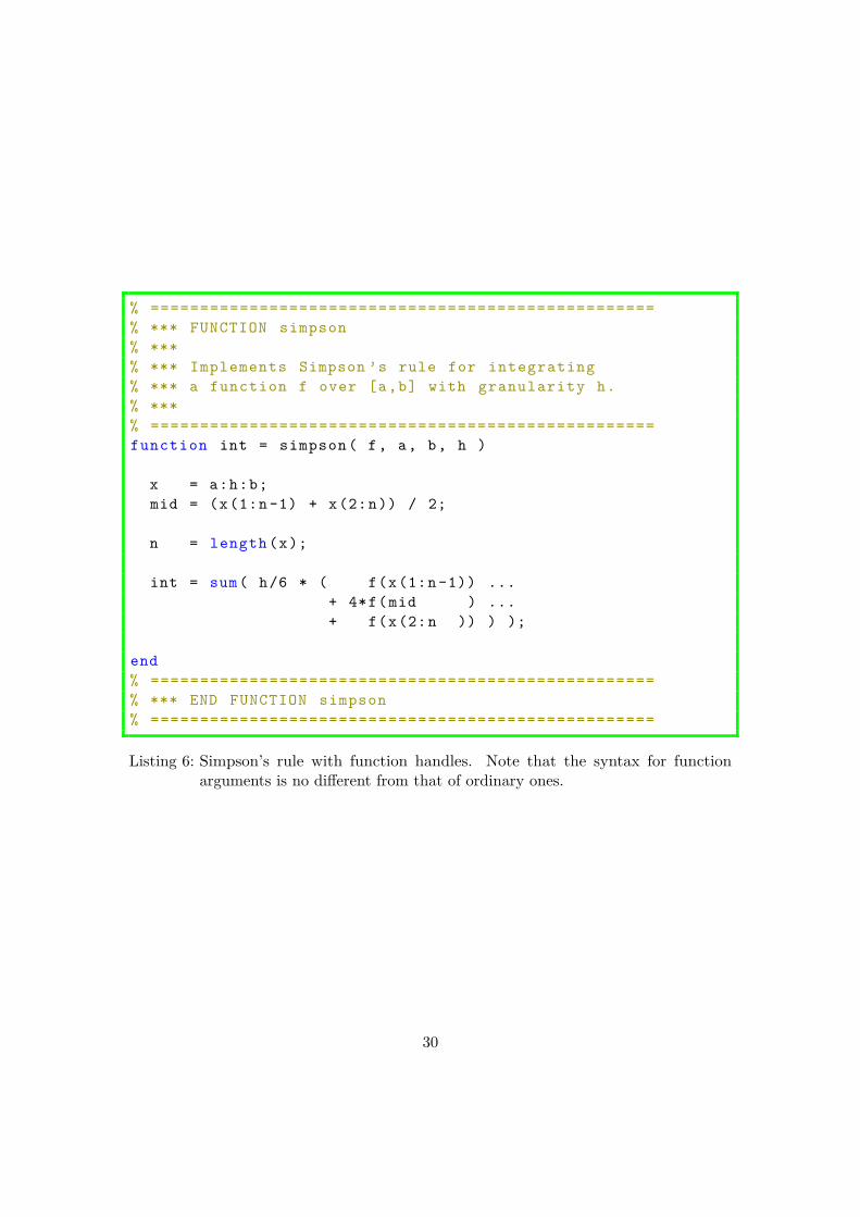
% ===================================================% *** FUNCTION simpson% ***% *** Implements Simpson ’s rule for integrating% *** a function f over [a,b] with granularity h.% ***% ===================================================function int = simpson ( f, a, b, h )

x = a:h:b;mid = (x(1:n -1) + x(2:n)) / 2;

n = length (x);

int = sum( h/6 * ( f(x(1:n -1)) ...+ 4*f(mid ) ...+ f(x(2:n )) ) );

end% ===================================================% *** END FUNCTION simpson% ===================================================

Listing 6: Simpson’s rule with function handles. Note that the syntax for functionarguments is no different from that of ordinary ones.

30

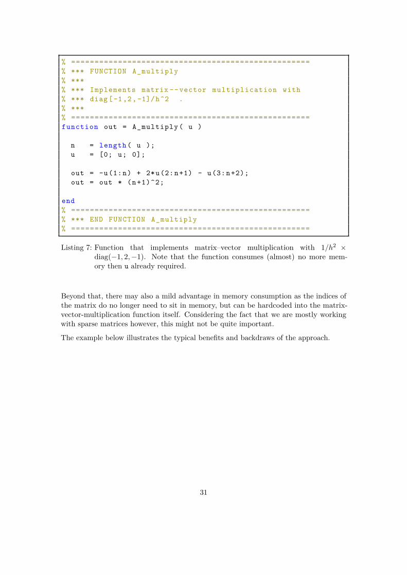
% ===================================================% *** FUNCTION A_multiply% ***% *** Implements matrix -- vector multiplication with% *** diag [-1,2,-1]/h^2 .% ***% ===================================================function out = A_multiply ( u )

n = length ( u );u = [0; u; 0];

out = -u(1:n) + 2*u(2:n+1) - u(3:n+2);out = out * (n +1)^2;

end% ===================================================% *** END FUNCTION A_multiply% ===================================================

Listing 7: Function that implements matrix–vector multiplication with 1/h2 ×diag(−1, 2,−1). Note that the function consumes (almost) no more mem-ory then u already required.

Beyond that, there may also a mild advantage in memory consumption as the indices ofthe matrix do no longer need to sit in memory, but can be hardcoded into the matrix-vector-multiplication function itself. Considering the fact that we are mostly workingwith sparse matrices however, this might not be quite important.

The example below illustrates the typical benefits and backdraws of the approach.

31

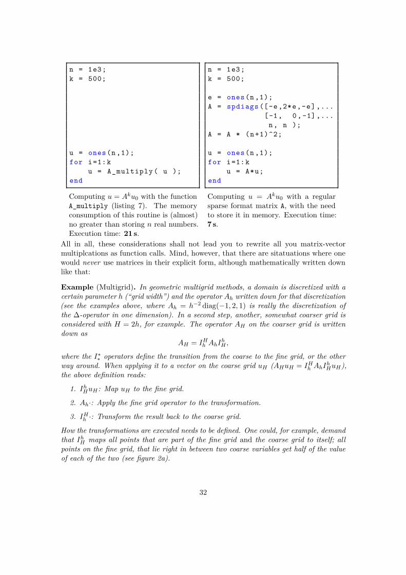
n = 1e3;k = 500;

u = ones(n ,1);for i=1:k

u = A_multiply ( u );end

Computing u = Aku0 with the functionA_multiply (listing 7). The memoryconsumption of this routine is (almost)no greater than storing n real numbers.Execution time: 21 s.

n = 1e3;k = 500;

e = ones(n ,1);A = spdiags ([-e ,2*e,-e] ,...

[-1, 0 , -1] ,...n, n );

A = A * (n +1)^2;

u = ones(n ,1);for i=1:k

u = A*u;end

Computing u = Aku0 with a regularsparse format matrix A, with the needto store it in memory. Execution time:7 s.

All in all, these considerations shall not lead you to rewrite all you matrix-vectormultiplcations as function calls. Mind, however, that there are sitatuations where onewould never use matrices in their explicit form, although mathematically written downlike that:

Example (Multigrid). In geometric multigrid methods, a domain is discretized with acertain parameter h (“grid width”) and the operator Ah written down for that discretization(see the examples above, where Ah = h−2 diag(−1, 2, 1) is really the discretization ofthe ∆-operator in one dimension). In a second step, another, somewhat coarser grid isconsidered with H = 2h, for example. The operator AH on the coarser grid is writtendown as

AH = IHh AhIhH ,

where the I∗∗ operators define the transition from the coarse to the fine grid, or the otherway around. When applying it to a vector on the coarse grid uH (AHuH = IHh AhIhHuH),the above definition reads:

1. IhHuH : Map uH to the fine grid.

2. Ah·: Apply the fine grid operator to the transformation.

3. IHh ·: Transform the result back to the coarse grid.

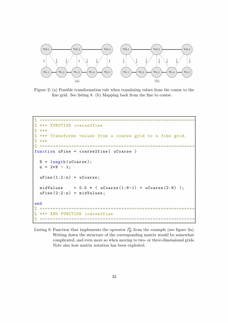
How the transformations are executed needs to be defined. One could, for example, demandthat IhH maps all points that are part of the fine grid and the coarse grid to itself; allpoints on the fine grid, that lie right in between two coarse variables get half of the valueof each of the two (see figure 2a).

32

uH,1 uH,2 uH,3

uh,1 uh,2 uh,3 uh,4 uh,5

1 12

12 1 1

212 1

(a)

uH,1 uH,2 uH,3

uh,1 uh,2 uh,3 uh,4 uh,5

12

14

14

12

14

14

12

(b)

Figure 2: (a) Possible transformation rule when translating values from the coarse to thefine grid. See listing 8. (b) Mapping back from the fine to coarse.

% ===========================================================% *** FUNCTION coarse2fine% ***% *** Transforms values from a coarse grid to a fine grid.% ***% ===========================================================function uFine = coarse2fine ( uCoarse )

N = length ( uCoarse );n = 2*N - 1;

uFine (1:2:n) = uCoarse ;

midValues = 0.5 * ( uCoarse (1:N -1) + uCoarse (2:N) );uFine (2:2:n) = midValues ;

end% ===========================================================% *** END FUNCTION coarse2fine% ===========================================================

Listing 8: Function that implements the operator IhH from the example (see figure 2a).Writing down the structure of the corresponding matrix would be somewhatcomplicated, and even more so when moving to two- or three-dimensional grids.Note also how matrix notation has been exploited.

33

In the analysis of the method, IhH and IHh will always be treated as matrices, but whenimplementing, one would certainly not try to figure out the structure of the matrix. It isa lot simpler to implement a function that executes the rule suggested above, for example.

References

[1] Peter J. Acklam. MATLAB array manipulation tips and tricks, October 2003. URLhttp://home.online.no/~pjacklam/matlab/doc/mtt/.

[2] Pascal Getreuer. Writing fast MATLAB code, 2009. URL http://www.mathworks.com/matlabcentral/fileexchange/5685.

[3] Doug Hull. Cleaner code in MATLAB, 2006. URL http://blogs.mathworks.com/pick/2006/12/13/cleaner-code-in-matlab-part-1-of-series/.

[4] Richard Johnson. MATLAB programming style guidelines, October 2002. URLhttp://www.mathworks.com/matlabcentral/fileexchange/2529.

[5] Mathworks. Code vectorization guide, 2009. URL http://www.mathworks.com/support/tech-notes/1100/1109.shtml.

[6] Cleve Moler. Numerical computing with MATLAB, 2004. URL http://www.mathworks.com/moler/chapters.html.

[7] Cleve Moler. Experiments with MATLAB, April 2008. URL http://www.mathworks.com/moler/exm/chapters.html.

34