A Xylophone Bar Magnetometer for micro/picosatellites

Herve Lamy∗, Veronique Rochus†, Innocent Niyonzima† and Pierre Rochus‡∗Belgian Institute for Space Aeronomy

Avenue Circulaire 3, 1180 Brussels, Belgium†Department of Aerospace and Mechanical Engineering,

University of Liege, Chemin des Chevreuils 1 (B52/3), 4000 Liege, Belgium‡Centre Spatial de Liege,

University of Liege, 4031 Angleur, Belgium

Abstract—The Belgian Institute of Space Aeronomy (BIRA-IASB), “Centre Spatial de Liege” (CSL), “Laboratoire de Tech-niques Aeronautiques et Spatiales” (LTAS) of University of Liege,and the Microwave Laboratory of University of Louvain-La-Neuve (UCL) are collaborating in order to develop a miniatureversion of a xylophone bar magnetometer (XBM) using Mi-croelectromechanical Systems (MEMS) technology. The deviceis based on a classical resonating xylophone bar. A sinusoidalcurrent is supplied to the bar oscillating at the fundamentaltransverse resonant mode of the bar. When an external magneticfield is present, the resulting Lorentz force causes the bar tovibrate at its fundamental frequency with an amplitude directlyproportional to the vertical component of the ambient magneticfield. In this paper we illustrate the working principles of theXBM and the challenges to reach the required sensitivity inspace applications (measuring magnetic fields with an accuracyof approximately of 0.1 nT). The optimal dimensions of theMEMS XBM are discussed as well as the constraints on thecurrent flowing through the bar. Analytical calculations as wellas simulations with finite element methods have been used.Prototypes have been built in the Microwave Laboratory usingSilicon on Insulator (SOI) and bulk micromachining processes.Several methods to accurately measure the displacement of thebar are proposed.

I. INTRODUCTION

Magnetic fields play a key role in many aspects of thesolar-terrestrial interactions. For example, during geomagneticactivity, charged particles precipitate along geomagnetic fieldlines and produce spectacular aurora. Strong sheets of field-aligned currents (FACs) associated with these precipitationsproduce local perturbations of the geomagnetic field. A mag-netometer onboard a spacecraft crossed by these current sheetswill record the magnetic field perturbations and will providea measure of the field aligned current using the Maxwell’sequation −→∇ ∧ −→B = −→J . With a single spacecraft stationarycurrent sheet may be obtained. However this situation is notalways observed. In some cases, spatial and temporal varia-tions of the magnetic field cannot be discriminated. Currentlythe separation of satellites in multi-spacecraft missions likeCluster or Themis is usually larger than the width of thecurrent sheet. This example illustrates the importance of multi-point measurements with a fleet of micro- or pico-spacecraftwith small separations.

Since launch costs represent a significant fraction of thetotal mission expenditures, reducing such costs necessitatescareful consideration of instrument and spacecraft componentminiaturization. The goal of this research is to build a sensitive,low mass, low size and low consumption magnetometer toembark onboard a fleet of micro-, nano- or pico-satellites inorder to carry out these multi-point measurements.

Three main types of magnetometers have been traditionallyused in space missions: the fluxgate magnetometer (FGM),the search-coil magnetometer (SCM) and the vector heliummagnetometer (VHM). Efforts to miniaturize size and massof these magnetic sensors have been limited by fabricationdifficulties and loss of sensitivity. Moreover, they are alwayslocated at the end of long booms to avoid magnetic perturba-tions from the spacecraft itself, a configuration that is hardlycompatible with nano- or pico-satellites.

In the framework of the Solar Terrestrial Center of Ex-cellence (STCE), the Belgian Institute for Space Aeronomy(BISA) is studying the feasibility of developing and construct-ing a magnetometer for space applications suited to miniatur-ization. With “Centre Spatial de Liege (CSL)”, “Laboratoire deTechniques Aeronautiques et Spatiales” (LTAS) of Universityof Liege, and Microwave Laboratory of University of Louvain-La-Neuve (UCL), the objective is to develop a Xylophone BarMagnetometer (XBM) in which the displacement of a beamis directly proportional to the magnitude of one componentof the ambient magnetic field. The specific design of thismagnetometer makes it particularly suitable to be fabricatedat the size of Microelectromechanical Systems (MEMS). Thisstudy benefits from previous works initiated at the AppliedPhysics Laboratory of the John Hopkins University (Givens etal 1996, Wickenden et al 1997, Zanetti et al 1998, Oursler etal 1999, Wickenden et al 2003).

The challenging task with this XBM is to reach thesubnanotesla accuracy and qualify it for space applications.Another goal we would like to achieve is to use a set ofsuch miniature magnetometers in a clever way to accuratelydetermine the electromagnetic contribution of the electronicsonboard a spacecraft. On one hand, this would reduce the mag-netic cleanliness requirements currently imposed on spacecraftinstruments and on the other hand, this would prevent the use

Fig. 1. Operating principle of a Xylophone Bar Magnetometer

of large booms for magnetometers.In section II, the working principles of the XBM are

described. An analytic study of the parameters influencingthe deflection of the bar is discussed in section III whilstsection IV is devoted to simulations with finite elementmethods (FEM). In section V, we describe a first XBM MEMSprototype manufactured at the Microwave Laboratory as wellas preliminary measurements of the curvature of the structure.Several methods to accurately measure the displacement ofthe bar are considered in section VI. We conclude with someperspectives about additional modeling with simulations.

II. WORKING PRINCIPLES OF THE XBM

The XBM magnetometer is based on a classical resonatingxylophone bar. This relatively simple device uses the Lorentzforce to measure one component of the ambient magnetic field.It consists of a thin conductive xylophone bar supported atthe nodes of its fundamental mode of mechanical vibration bytwo arms bonded to the bar to provide low-resistance electricalcontacts (see Figure 1). The nodes are located at 22.4% of thebar’s length from each unclamped end.

A sinusoidal current is supplied to the bar through thesearms, oscillating at the fundamental transverse resonant modeof the bar f0:

f0 =22.42π

√EIaω L4

=1.029 bL2

√E

ρ(1)

where E is the Young’s modulus (N/m2), L the bar length,Ia the area moment of inertia (= ab3/12 for a rectangularbeam), ω the mass per unit length (ρ = ω a b), and ρ, a, b arethe mass density, width and thickness of the bar, respectively.When a current I is driven through the xylophone bar in thepresence of an external magnetic field Bext, a resulting Lorentzforce applied to the bar makes it vibrate vertically.

~F = I ~Ls ∧ ~Bext (2)

where ~Ls is a vector whose magnitude Ls is the lengthof the xylophone bar between the supports (Ls ∼ 0.552L).When the frequency of the current is set at the fundamentaltransverse resonant frequency of the bar, the deflection of the

bar is strongly enhanced and its amplitude in the middle ofthe bar is given by

d(f0) =5F L4

s

384E IaQ = 1.206× 10−3 × FL4

E IaQ (3)

where Q is the mechanical quality factor which is deter-mined by different parameters depending on bar material,manufacturing process, but also includes various types ofdampings such as air damping, support damping, thermoelasticdamping and surface damping. Equation (3) is obtained bymodeling the bar as a mass-spring-dashpot system submittedto a static deformation. Another approach to obtain the theo-retical displacement of the bar is to solve the Euler-Bernouilliequation of a free-free bar submitted to a dynamic deformation(Niyonzima 2009). In this case, the displacement of the bar isgiven by

d(f0) = 1.747× 10−3 × FL4

E IaQ (4)

The ratio between equations (4) and (3) is equal to 1.446.Both theoretical values will be compared to values obtainedwith simulations in section IV.

From equations (2), (3) and (4), it can be seen that theamplitude of the deflection of the bar is linearly proportionalto the magnetic field component B parallel to the surface of thexylophone bar and normal to the direction of the drive current.This device is therefore intrinsically linear unlike many othermagnetometers. In principle, it also has a very wide dynamicalrange: magnetic field intensities from nanoteslas to teslascould be measured by simply adjusting the current amplitude.However, the maximum intensity of the current that can flowthrough the bar depends on the importance of the Jouleeffect and of the thermomechanical coupling. Indeed, a toolarge elevation of temperature inside the bar could result insignificant modifications of its mechanical properties. Thisthermomechanical coupling is briefly discussed in section IVdevoted to simulations. The influence of the other parametersof the bar (dimensions, Young modulus, quality factor) on itsdeflection are discussed in section III.

Because the other vibration modes of the bar have a verydifferent frequency and are not excited at this frequencyf0, this technique discriminates against these components ofthe magnetic field extremely well so that any second-ordercross coupling between different field components is extremelysmall. A three-axis sensor can be constructed with threexylophone bars operating at different frequencies.

The variation of the amplitude of the bar deflection as afunction of the frequency of the driving current in a constantexternal magnetic field B is given by

d = d(f0) × 1√[1− ( ff0 )2]2 + ( f

Qf0)2

(5)

As the frequency is chosen as the fundamental mechanicalresonance frequency, the displacement amplitude is enhanced,

reaching a maximum value given by d(f0), while the phaseangle displays a 180 shift.

The amplitude of the deflection of the xylophone bar can bemeasured by established detection techniques such as opticaland capacitive methods or by new techniques using plasmonsor magnetostrictive material. They will be shortly discussed insection VI.

III. PARAMETRIC STUDY OF THE DEFLECTION

In this section we discuss different parameters influencingthe deflection d, namely, the electric current I , the Youngmodulus E, the quality factor Q and the dimensions L, aand b of the bar.

A. Influence of the current: Joule effect and thermoelectriccoupling

According to equation (3) or (4), the larger the currentflowing through the bar, the larger its deflection. However, themaximum value of the electrical current flowing into the bar isin practice limited by the Joule effect and the thermomecanicalcoupling. The increase of temperature resulting from the Jouleeffect can on one hand modify the thermal and electricalconductivites of the material (respectively κ and σ), and onanother hand the mechanical properties of the bar via thethermal coefficient of expansion α (which can modify thedimensions of the structure, therefore its eigenfrequencies)or via the Young’s modulus. These couplings can better beaccounted for with FEM simulations. In section IV, a simplermethod will be used with a mechanical calculation carried outafter a thermo-electromagnetic study.

However, as a first step, we make a simple estimation of themaximal value of the current Imax by using an electric circuitanalogy of the system insulator+bar+arms. In this analogy,conduction heat transfer is modeled with thermal resistancesRx = wx

κx Sxwhere x stands either for the insulator, the arm or

the bar. w is the width, κ the thermal conductivity and S thecross section. A discrete distribution of temperature is assumedin several nodes (see Fig 2). The temperature profile isdetermined by solving a set of Kirchoff laws at the nodes whena voltage is applied through the arms. This temperature profileis then used to update the values of electric and thermal con-ductivitites. Electric resistivity was represented by an empiricallinear relationship ρ = ρ0× (1 + α (T − T0)) where ρ0 is theresistivity at the room temperature T0 (ρ0 ∼ 2, 28×10−8 Ω mand α ∼ 0.004 K−1 in the case of Aluminium). The thermalconductivity κ was then calculated with the Wiedemann-Franzlaw

κ

σ T=π2 k2

b

3 e2(6)

where kb and e are respectively the Boltzmann constantand the charge of the electron. This empirical law is validin metals where the heat conduction is mainly ensured byfree electrons. It would not be valid in semi-conductors likesilicon where heat conduction is also due to phonons. Also,experiments have shown that it is valid at high and low

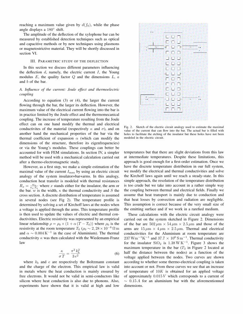
Fig. 2. Sketch of the electric circuit analogy used to estimate the maximalvalue of the current that can flow into the bar. The actual bar is filled withholes to facilitate the etching of the insulator but these holes have not beenmodeled in the electric circuit.

temperatures but that there are slight deviations from this lawat intermediate temperatures. Despite these limitations, thisapproach is good enough for a first-order estimation. Once wehave the discrete temperature distribution in our full system,we modify the electrical and thermal conductivities and solvethe Kirchoff laws again until we reach a steady-state. In thissimple approach, the resolution of the temperature distributionis too crude but we take into account in a rather simple waythe coupling between thermal and electrical fields. Finally weassume that heat transport is mainly due to conduction andthat heat losses by convection and radiation are negligible.This assumption is correct because of the very small size ofthe emitting surface and if we work in a rarefied medium.

These calculations with the electric circuit analogy werecarried out on the system sketched in Figure 2. Dimensionsof the bar are 502µm × 54µm × 2.5µm and those of thearms are 15µm × 4µm × 2.5µm. Thermal and electricalconductivities for the Aluminium at room temperature are237 Wm−1K−1 and 37.7 × 106 S m−1. Thermal conductivityfor the insulator SiO2 is 1.38 W K−1. Figure 3 shows themaximum temperature in the bar (T3 in Figure 2 located athalf the distance between the nodes) as a function of thevoltage applied between the nodes. Two curves are shownaccording to whether some thermo-electrical coupling is takeninto account or not. From these curves we see that an increaseof temperature of 10K is obtained for an applied voltageof approximately 0.015V which corresponds to a current of∼ 0.15A for an aluminium bar with the aforementionneddimensions.

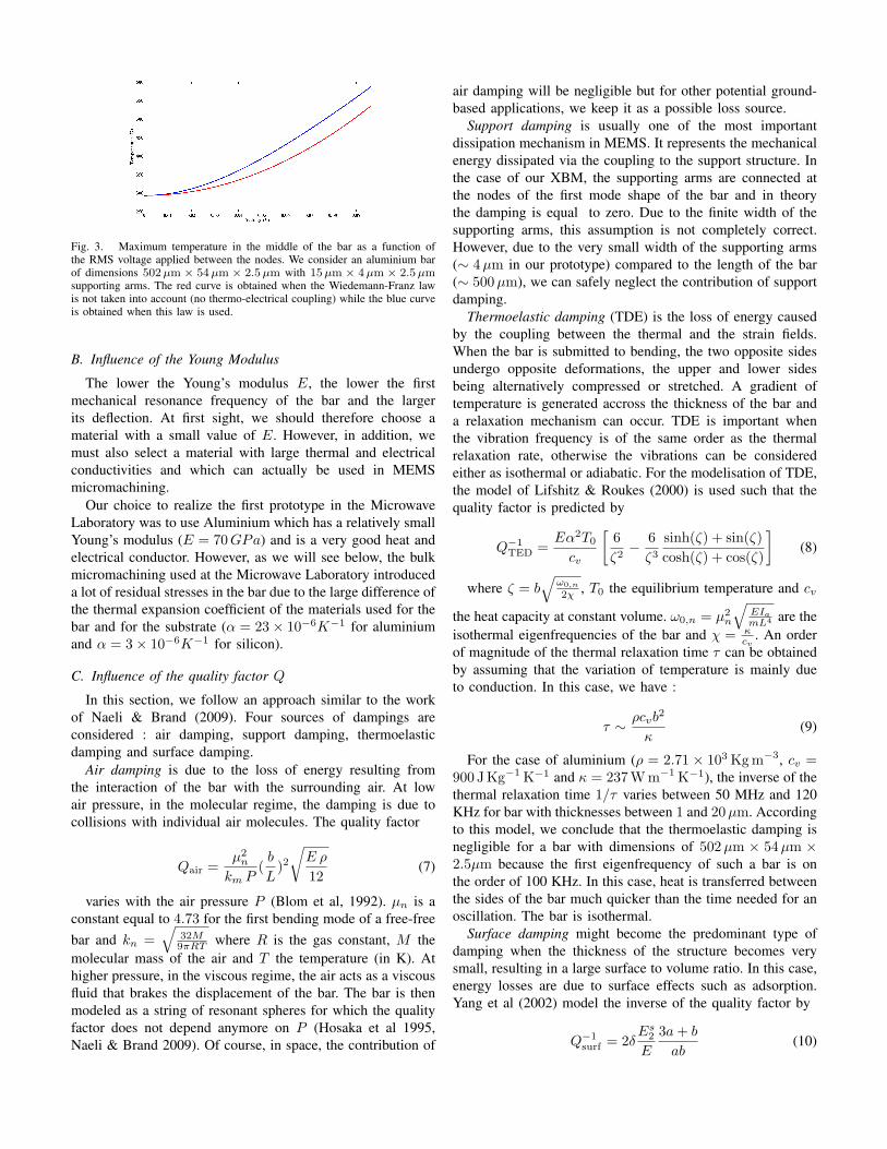
Fig. 3. Maximum temperature in the middle of the bar as a function ofthe RMS voltage applied between the nodes. We consider an aluminium barof dimensions 502µm × 54µm × 2.5µm with 15µm × 4µm × 2.5µmsupporting arms. The red curve is obtained when the Wiedemann-Franz lawis not taken into account (no thermo-electrical coupling) while the blue curveis obtained when this law is used.

B. Influence of the Young Modulus

The lower the Young’s modulus E, the lower the firstmechanical resonance frequency of the bar and the largerits deflection. At first sight, we should therefore choose amaterial with a small value of E. However, in addition, wemust also select a material with large thermal and electricalconductivities and which can actually be used in MEMSmicromachining.

Our choice to realize the first prototype in the MicrowaveLaboratory was to use Aluminium which has a relatively smallYoung’s modulus (E = 70GPa) and is a very good heat andelectrical conductor. However, as we will see below, the bulkmicromachining used at the Microwave Laboratory introduceda lot of residual stresses in the bar due to the large difference ofthe thermal expansion coefficient of the materials used for thebar and for the substrate (α = 23× 10−6K−1 for aluminiumand α = 3× 10−6K−1 for silicon).

C. Influence of the quality factor Q

In this section, we follow an approach similar to the workof Naeli & Brand (2009). Four sources of dampings areconsidered : air damping, support damping, thermoelasticdamping and surface damping.

Air damping is due to the loss of energy resulting fromthe interaction of the bar with the surrounding air. At lowair pressure, in the molecular regime, the damping is due tocollisions with individual air molecules. The quality factor

Qair =µ2n

km P(b

L)2√E ρ

12(7)

varies with the air pressure P (Blom et al, 1992). µn is aconstant equal to 4.73 for the first bending mode of a free-freebar and kn =

√32M9πRT where R is the gas constant, M the

molecular mass of the air and T the temperature (in K). Athigher pressure, in the viscous regime, the air acts as a viscousfluid that brakes the displacement of the bar. The bar is thenmodeled as a string of resonant spheres for which the qualityfactor does not depend anymore on P (Hosaka et al 1995,Naeli & Brand 2009). Of course, in space, the contribution of

air damping will be negligible but for other potential ground-based applications, we keep it as a possible loss source.

Support damping is usually one of the most importantdissipation mechanism in MEMS. It represents the mechanicalenergy dissipated via the coupling to the support structure. Inthe case of our XBM, the supporting arms are connected atthe nodes of the first mode shape of the bar and in theorythe damping is equal to zero. Due to the finite width of thesupporting arms, this assumption is not completely correct.However, due to the very small width of the supporting arms(∼ 4µm in our prototype) compared to the length of the bar(∼ 500µm), we can safely neglect the contribution of supportdamping.

Thermoelastic damping (TDE) is the loss of energy causedby the coupling between the thermal and the strain fields.When the bar is submitted to bending, the two opposite sidesundergo opposite deformations, the upper and lower sidesbeing alternatively compressed or stretched. A gradient oftemperature is generated accross the thickness of the bar anda relaxation mechanism can occur. TDE is important whenthe vibration frequency is of the same order as the thermalrelaxation rate, otherwise the vibrations can be consideredeither as isothermal or adiabatic. For the modelisation of TDE,the model of Lifshitz & Roukes (2000) is used such that thequality factor is predicted by

Q−1TED =

Eα2T0

cv

[6ζ2− 6ζ3

sinh(ζ) + sin(ζ)cosh(ζ) + cos(ζ)

](8)

where ζ = b√

ω0,n

2χ , T0 the equilibrium temperature and cv

the heat capacity at constant volume. ω0,n = µ2n

√EIa

mL4 are theisothermal eigenfrequencies of the bar and χ = κ

cv. An order

of magnitude of the thermal relaxation time τ can be obtainedby assuming that the variation of temperature is mainly dueto conduction. In this case, we have :

τ ∼ ρcvb2

κ(9)

For the case of aluminium (ρ = 2.71 × 103 Kg m−3, cv =900 J Kg−1 K−1 and κ = 237 W m−1 K−1), the inverse of thethermal relaxation time 1/τ varies between 50 MHz and 120KHz for bar with thicknesses between 1 and 20µm. Accordingto this model, we conclude that the thermoelastic damping isnegligible for a bar with dimensions of 502µm × 54µm ×2.5µm because the first eigenfrequency of such a bar is onthe order of 100 KHz. In this case, heat is transferred betweenthe sides of the bar much quicker than the time needed for anoscillation. The bar is isothermal.

Surface damping might become the predominant type ofdamping when the thickness of the structure becomes verysmall, resulting in a large surface to volume ratio. In this case,energy losses are due to surface effects such as adsorption.Yang et al (2002) model the inverse of the quality factor by

Q−1surf = 2δ

Es2E

3a+ b

ab(10)

Fig. 4. Inverse quality factors as a function of pressure for air damping,thermoelastic damping and surface damping. Calculations have been carriedout for a 502µm × 54µm × 2.5µm bar with 15µm × 4µm × 2.5µmsupporting arms. Temperature is 293K.

Fig. 5. Quality factor of an aluminium bar as a function of the length. Widtha = 54µm and thickness b = 2.5µm. Dimensions of supporting arms are15µm× 4µm× 2.5µm. Temperature is 293K.

where Es2 is a property of the adsorbate layer. Someexperiments on 20µm thick beams have shown that theproduct δ Es2 is close to 1, a value that we will assume inthe following. The exact value of this parameter has to bedetermined experimentally.

Taking into account the various dampings, the total qualityfactor is calculated as

Q−1tot = Q−1

air +Q−1TED +Q−1

surf (11)

where we have already neglected the support damping.Figure 4 illustrates the inverse of the quality factor as afunction of the pressure for the three damping mechanisms.At low pressure, air damping becomes negligible. The majorparameter that will then determine whether TED or surfacedamping dominates is the thickness of the bar. For ourXBM, the thickness is small and so the surface damping willbe predominant. Since this mechanism is poorly describedanalytically, the actual quality factor will have to be carefullymeasured experimentally.

D. Influence of the dimensions of the bar

In equation (3), the deflection of the bar is a function of itsdimensions via L (or Ls), the area moment of inertia Ia andthe quality factor Q. Figures 5, 6 and 7 respectively illustratethe variation of the quality factor with the length L, the widtha and the thickness b of the bar. Two cases are shown : no airpressure and air pressure of 10−3 bar (=103 Pa).

The displacement of the bar increases strongly when thelength of the bar increases due to the L4 dependance. For

Fig. 6. Quality factor of an aluminium bar as a function of the width. LengthL = 502µm and thickness b = 2.5µm. Dimensions of supporting arms are15µm× 4µm× 2.5µm. Temperature is 293K.

Fig. 7. Quality factor of an aluminium bar as a function of the thickness.Length L = 502µm and width a = 54µm. Dimensions of supporting armsare 15µm× 4µm× 2.5µm. Temperature is 293K.

non-zero pressure, there is an optimal value of the length(L ∼ 500µm giving the highest possible quality factor(see Figure 5). Of course the length of the bar cannot belarger than a maximum value above which the bar will stickto the substrate. The width of the bar has relatively fewimportance both on the quality factor (see Figure 6) and on thedisplacement of the bar (because the dependance of Ia with ais only linear) but it must be at least of the order of 50µm tohave the largest Q value. The simulations presented in sectionIV will also indicate that the width is important for the correctcalculation of the bar eigenfrequencies. Finally, there is also anoptimal value of the thickness (b ∼ 2.5µm) which maximizesthe quality factor (see Figure 7). The thickness also has astrong impact on the displacement of the bar because of theb3 dependance of the Ia factor. Thinner bars produce largervalues of the bar displacement.

Therefore, in the simulations presented below, the length ofthe bar L will always be of the order of 500µm, the width ofthe bar a of the order of 50µm and the thickness of the barb lower or equal to 2.5µm.

IV. SIMULATIONS WITH FINITE ELEMENT METHODS

These FEM simulations have been carried out with Oofeliedriven by Samcef. Oofelie is a finite element multi-physicssoftware which allows to model the couplings between variousfields. In the XBM, the sinusoidal electric current flowingthrough the bar induces a temperature increase via a Jouleeffect, which also modifies the thermal and electrical conduc-tivities of the bar and therefore changes the current distributioninside the bar. There is a thermo-electromagnetic coupling.

The temperature increase inside the bar can also modify itsmechanical properties such as its dimensions and its Youngmodulus, and therefore its eigenfrequencies. We adopted thefollowing procedure: first, a thermo-electromagnetic steady-state equilibrium is computed. Then, the eigenfrequencies ofthe bar are calculated by assuming small perturbations of thissteady state and carrying out a linear analysis around theequilibrium solution.

Due to the symmetry of the XBM, all these simulationswere done only on a quarter of the whole structure (one halfin length and one half in width) to save computational time.

A. Influence of the holes in the bar

As will be described in section V, the bar in our MEMSXBM prototype is designed with many holes (see also Figure2 for a sketch) in order for the etchant to easily access thesacrificial SiO2 layer and release the structure during themicromachining process. The dimensions of these holes are2µm× 2µm and their separation is 5µm. So, before runningthe simulations described above, a mechanical simulation iscarried out to check their influence on the calculations ofthe eigenfrequencies. Furthermore, since the presence of theseholes strongly increase the computational time (because thesize of the mesh must be smaller than the size of a hole), it ishighly desirable to make simulations with a full structure (withno holes) instead of the more complicated structure with holes.For that purpose a comparison is made between the valuesof the first eigenfrequency obtained with two mechanicalsimulations : the first one is obtained for the structure withholes using a finer mesh size while the second is obtained forthe full structure with no holes but with electrical, mechanicaland thermal properties modified as follows :

x = x0 ×VhV0

(12)

where Vh is the volume of the bar with holes and V0 is thevolume of the bar without holes. x stands for the electricalconductivity σ, the thermal conductivity κ, the Young modulusE or the density of the bar ρ. The two simulations areillustrated in Figures 8 and 9 obtained for a bar with thesame dimensions. The difference between the values of thefirst eigenfrequencies obtained with the two simulations is onlyof 45 Hz. We can then safely use a full structure with adaptedmaterial parameters for the following simulations.

B. Electromagnetic calculations

A general electromagnetic calculation implies to solve theMaxwell equations

~∇∧ ~H = ~j +∂ ~D

∂t(13)

~∇∧ ~E = −∂B∂t

(14)

for the geometry given by one quarter of the bar + support-ing arms. However, for our problem, additional assumptions

Fig. 8. Calculation of the first eigenfrequency of a structure with2µm × 2µm holes separated by a distance of 5µm. Dimensions of thebar are 427µm × 54µm × 2.5µm and those of the supporting arms are5µm× 4µm× 2.5µm. The first eigenfrequency is f = 99.122 MHz.

Fig. 9. Calculation of the first eigenfrequency of a structure with no holesand the same dimensions as in Figure 8. The properties of the material havebeen modified according to (12). The first eigenfrequency is f = 99.077MHz.

apply which simplify the Maxwell’s equations. First, capaci-tive effects can be neglected, i.e. the displacement current ∂ ~D∂tis negligible. This assumption holds because the size of thebar L λ, the wavelength which is of the order of 3000 mfor a vibration frequency of ∼ 100 KHz. Second, skin effectsare negligible. Indeed the skin depth of the aluminium barwith the above dimensions is of the order of 300µm, muchlarger than the thickness of the bar. In this case, the generalelectromagnetic problem reduces to an electrokinetic one andthe Maxwell’s equations become

~∇.~j = 0 (15)

~∇∧ ~E = 0 (16)

From (15), the distribution of the current density throughoutthe bar can be calculated with adequate boundary conditions.Parallel electromagnetic boundary counditions were applied onexternal faces of the structure to simulate a null electromag-netic field at infinity. An example is shown in Figure 10. Thedistribution of the voltage along the structure can be obtainedfrom (16). Finally the distribution of the magnetic field aroundthe structure induced by the current flowing in the bar can alsobe calculated.

C. Thermal calculations

From the distribution of the current density ~j, a thermalcalculation can be performed assuming that heat is transmittedonly by conduction. Neglecting thermal radiation is a valid

Fig. 10. Distribution of the current density in the bar obtained with Oofelieby solving an electrokinetic problem. Only one quarter of the bar is shown.

Fig. 11. Distribution of the temperature in a bar with dimensions 427µm×49µm×2.5µm and supporting arms of dimensions 15µm×4µm×2.5µm.Applied voltage between the nodes is ∆V = 0.0181 V.

assumption given the size of the bar. Since we are notinterested in the complete dynamical process but instead in thefinal thermo-electric steady-state equilibrium, only the steady-state equation of heat conduction is solved :

~∇.(κ ~∇T ) = −Qv (17)

Qv is the power per unit volume generated as heat bythe Joule effect. As mentionned above, in those simulations,the coupling between electric and thermal fields is neglected.An example of result is shown in Figure 11 for a bar withdimensions 427µm × 49µm × 2.5µm and supporting armsof dimensions 15µm × 4µm × 2.5µm. The applied voltagebetween the nodes was ∆V = 0.0181 V, corresponding to acurrent of ∼ 0.15 A. The maximum value of the temperaturein the structure obtained with simulations is 296K, which issmaller than the value (301.5K) obtained with the equivalentelectric circuit method described in section II. The differencemight be due to the lack of thermo-electrical coupling in oursimulations but also to the too crude discretisation of the bar inthe equivalent electric circuit. The discrepancy between resultsfrom the two methods increases when the applied voltagebecomes larger. Figure 12 shows a profile in the temperaturedistribution in the bar taken at half the width of the bar.

D. Mechanical calculations

Firstly, the first eigenfrequency and the related mode shapeare evaluated using the piezoelectric module of Oofelie. Theexternal load applied to the bar is the Lorentz force, ~F =~j∧ ~Bext, whose distribution along the bar is calculated from the

Fig. 12. Temperature profile along the bar corresponding to results shownin Figure 11. The cross section is located at half the width of the bar.

distribution of the current density ~j and from a given value ofthe external magnetic field ~Bext. The following finite elementsequation is solved :

M ~q + C ~q +K ~q = ~F (18)

M , C, and K respectively represent the mass matrix, thedamping matrix and the spring matrix. ~F and ~q are respectivelythe vectors of applied forces and of the displacements ofnodes/elements. For the damping matrix C, a proportionaldamping was assumed, i.e. C = a1M + a2K, from whichwe obtain 1

2Q ' ε = 12ω a1 + 1

2a2 ω, where ε is the dampingratio. Q can be found either with analytical calculations (ashas been done in section III) or by evaluating it with dynamicsimulations (see determination of the thermoeleastic dampingbelow). From Q, the values of a1 and a2 to use in thesimulations can be determined.

The size of the mesh must be checked in order to see ifthe discretisation of the system is good enough. For that pur-pose, the first eigenfrequency is calculated with an increasingnumber of elements until it converges. The discretisation issufficient when convergence is reached. Tetrahedral elementsare used. Equation (18) is solved with a Cholesky LU factor-ization solver. Convergence was better achieved with secondorder elements. Typical number of elements needed to reachconvergence is of the order of 105.

Then, a frequency sweep around the first eigenfrequencyis carried out to study the dynamic behavior of the bar. Anexample is shown in Figure 13 where the deflection of the baris shown as a function of the frequency for a given value ofQ = 10000. The simulations results are in better agreementwith the theoretical curve given by equation (3).

On the other hand, the theoretical value of the first eigen-frequency, given by equation (1), is very different from thevalue obtained with Oofelie simulations. This is highlightedin table I where theoretical and simulated values of the firsteigenfrequency have been calculated for various lengths of thebar. The discrepancy between the theoretical and simulatedvalues are probably due to the fact that the true geometry ofthe bar is more complex than a free-free bar.

Table II compares theoretical and simulated values of thefirst eigenfrequencies of the bar for several values of the barwidth. The theoretical value given by (1) is independent of thewidth of the bar. However, simulations show that the width of

Fig. 13. Deflection of the bar as a function of the frequency for a given valueofQ = 10000. Dimensions of the aluminium bar are 411µm×54µm×1µmand those of the supporting arms are 5µm×4µm×1µm . The correspondingfirst eigenfrequency is 55, 817 KHz. Dots are values of simulations obtainedwith Oofelie. The red curve is the theoretical dynamical response given byequation (3) while the blue curve is the theoretical dynamical response givenby equation (4).

Length Theorerical value Simulation value

µm KHz KHz

215 283.405 343.380313 133.709 171.452411 77.553 104.439509 50.564 71.165607 35.555 52.130705 26.357 40.183803 20.316 32.179901 16.135 26.549

TABLE ITHEORETICAL AND NUMERICAL VALUES OF THE FIRST

EIGENFREQUENCIES AS A FUNCTION OF THE LENGTH OF AN ALUMINIUMBAR WITH WIDTH a = 54µm, THICKNESS b = 2.5µm, AND WITH

15µm× 4µm× 2.5µm SUPPORTING ARMS.

Width Theorerical value Simulation value

µm KHz KHz

26 51.984 88.46254 51.984 70.323103 51.984 64.374152 51.984 61.228201 51.984 59.400

TABLE IITHEORETICAL AND NUMERICAL VALUES OF THE FIRST

EIGENFREQUENCIES AS A FUNCTION OF THE WIDTH OF AN ALUMINIUMBAR WITH LENGTH L = 502µm, THICKNESS b = 2.5µm, AND WITH

15µm× 4µm× 2.5µm SUPPORTING ARMS.

the bar is an important parameter for the determination of theeigenfrequencies, supporting the idea that our system cannotbe modelled by a simple free-free bar.

Finally, let us note that the sinusoidal current in the barinduces a magnetic field around it which in magnitude maybe much larger than the external magnetic field we wish tomeasure. However, this induced magnetic field also variessinusoidally and the resulting Lorentz force varies thereforeas ∼ sin2 ωt ∝ 1+cos 2ωt

2 . As a consequence, this force is notamplified since it has a static component and a component

vibrating at twice the first eigenfrequency of the structure.Moreover, the distribution of the induced magnetic field issymmetric if the shape of the bar is symmetric. Duringsmall displacements, this symmetry is slightly broken but theeffect is very small. On the other hand, if there are largerasymmetries in the bar due to the micromachining process, theinfluence of the induced magnetic field can set up an upperlimit on the smallest value of the external magnetic field thatcan be measured with this technique.

E. Multi-layer structures

A prototype bar with multi-layer structure has also beenmanufactured at the Microwave Laboratory of UCL (seeSection V). Therefore simulations with multi-layer structures(2 or 3) were also carried out with Oofelie, one layer beingmade of aluminium and the other ones made of less conductivematerial such as silicon or silicon nitride (Si3N4).

1) Electromagnetic and thermal calculations: The electro-magnetic and thermal simulations can be done similarly asfor monolayer structures. The current density ~j is mainlydistributed within the most conductive material (aluminium).Thermal fluxes are also predominant in the aluminium layer.

2) Mechanical calculations: Eigenfrequencies increase inmulti-layer structures in comparison to the values obtained formono-layer structures. For example, for a 411µm× 54µm×1µm with 5µm×4µm×1µm supporting arms, the first eigen-frequency is 55.818 KHz for a mono-layer structure, 89.358KHz for a two-layer aluminium/silicon nitride structure and92.609 KHz for a three-layer aluminium/silicon nitride/siliconstructure.

With multi-layer structures, residual stresses can occur dueto intrinsic or extrinsic phenomena. To establish the accuratedistribution of these stresses is a very complicated task whichcan be modeled with FEM simulations only if exact detailsof the manufacturing processes are known. As a first step, asimpler approach is undertaken : only residual stresses dueto a mismatch between aluminium and silicon nitride thermalcoefficients is considered. Figure 14 illustrates the deformationof a bi-layer structure due to cooling from 150C, the deposi-tion temperature for aluminium, to an ambient temperatureof 20C. The nitride layer undergoes compressive stresseswhile the aluminium one undergoes tensile stresses. The firsteigenfrequency is shifted from ∼ 90 KHz for the structurewithout these residual stresses to ∼ 105 KHz when theseresidual stresses are taken into account. Further simulationsincluding detailed residual stresses in the bar will be importantto accurately model the dynamic behavior of the structure.

Finally, even though TED is negligible in mono-layer struc-ture with thicknesses lower or equal to 2.5µm, it has to bechecked for bi-layer and three-layer structures. We assumeother types of dampings are negligible. The pyropiezoelectricmodule of Oofelie is used as it allows couplings betweenthermal and mechanical fields and therefore the prediction ofthe TED. A frequency sweep around the first eigenfrequencywith ∆f = 7 Hz gives the deformation of the bar as a function

Fig. 14. Deformation of a 411µm× 54µm× 1.25µm bar with 5µm×4µm× 1.25µm supporting arms. The structure has two layers : 1µm layerof aluminium and 0.25µm layer of silicon nitride.

Fig. 15. Deformation of a 411µm×54µm×1.25µm two-layer bar (1µmlayer of aluminium and 0.25µm layer of silicon nitride) with 5µm×4µm×1.25µm supporting arms, as a function of the frequency. ∆f = 7Hz.

of the frequency. Results for a 411µm×54µm×1.25µm two-layer bar (1µm layer of aluminium and 0.25µm of nitride)with 5µm × 4µm × 1.25µm supporting arms are shown inFigure 15. The value of the quality factor Q is obtained from

Q =ω0

∆ω(19)

where ω0 is the frequency of the peak deformation dmax

and ∆ω is the frequency width at a value of dmax√2

. A valueof Q = 12765 is found. For comparison, in mono-layerstructures, a value of Q ∼ 558000 is found for a structure withthe same dimensions (except the thickness b was equal to 1µmand made only of aluminium) and with the same assumptions(no other type of dampings). For a three-layer structure withthe same dimensions and a thickness of 1.35µm (1µm ofaluminium, 0.25µm of silicon nitride and 0.1µm of silicon),the value of the quality factor is Q = 13153. Thermoelasticdamping is therefore an important source of damping in thesemulti-layer structures.

V. FABRICATION OF A XBM PROTOTYPE

Following the parametric study and the simulations ofthe XBM, prototypes have been realized in the MicrowaveLaboratory of UCL. Two fabrication processes have beenused : Silicon-On-Insulator (SOI) and bulk. Several materialswere used, including aluminium, silicon and insulators suchas silicon nitride (Si3N4) and silicon oxide (SiO2). With both

Fig. 16. Design of the different layers used in the various fabricationprocesses for the XBM prototype

processes, the curvature of the structure must be as small aspossible. Curvature of the structure may arise due to stressgradients developing along the thickness of mono- or multi-layer structures. The origin of these stress gradients can beeither intrinsic or extrinsic. In the latter case, they are due toa difference in the thermal expansion coefficients between thevarious layers constituting the structure. Indeed, these layersare deposited at high temperature and contract differently whenthey cool down. This creates stresses because the layers sticktogether.

Figure 16 illustrates the three classes of structures designedfor the XBM prototype. For the SOI structures, we start witha material made of 100 nm silicon layer - 250 nm SiO2 layer -380µm silicon (substrate) on top of which is deposited a 250nm LPCVD (low pressure chemical vapor deposition) siliconnitride film. A mask is used to etch both the nitride and siliconlayers using positive litography. An 880 nm thick aluminiumlayer is then deposited on top of the structure with an electrongun deposition technique. The oxide layer is finally removedusing HF.

For bulk processes, there are two different types of struc-tures. In both types, a thick bulk silicon layer is the substrateon top of which a 400 nm silicon oxide film is deposited.In the first type of structure, a 1000 nm aluminium film isdeposited using the electron gun deposition technique, thenthe SiO2 film is etched. In the second type of structures, a250 nm LPCVD nitride film is deposited between the siliconoxyde film and the aluminium layer. It is etched before theoxide film.

With bulk micromachining processes, the use of aluminiumwhich has much larger electric and thermal conductivites thansilicon increases the maximum value of current which can flowthrough the bar, and therefore increase the sensitivity of thedevice. However, an important drawback is that large residualstresses remain after the fabrication process compared to thoseobserved in SOI structures. These stresses are mainly due tothe large difference of thermal expansion coefficients betweenthe silicon substrate and the aluminium layer.

In addition to the three different structures described above,several lengths and widths of the bar are considered. Squareholes of dimensions 2µm × 2µm and spaced by 5µm havebeen included in the design to allow the etching of theinsulating layer underneath the structure to release it.

These XBM prototypes will be tested soon at the LTAS andresults will be compared to the analytical results and the simu-

Fig. 17. Topography of one of the MEMS XBM prototype obtained withwhite-light interferometry technique.

lations obtained with Oofelie. Measurements of the dimensionsof the curvature of the structure have been conducted at UCLwith the Polytec MSA-500 machine which uses white-lightinterferometry techniques to measure the topography of thestructure. An example is shown in Figure 17. The structureis strongly curved in the central part, with an elevation of afew µm. Future measurements will have to determine howthe curvature of this structure affects the determination of theeigenfrequencies of the bar as well as its displacement.

VI. METHODS FOR DETECTING THE BAR DEFLECTION

According to equation (3), if we know the dimensions ofthe bar, the Young modulus of the material, the electric currentflowing through the device and the mechanical quality factorat the resonance, one component of the external magneticfield can be determined from the measurement of the bardisplacement d. In this section, we review a number of well-established detection techniques which can be used to measurethis displacement such as optical and capacitive methods. Wealso briefly consider potentially interesting new techniquessuch as surface plasmons resonance and the use of a mag-netostrictive material for the bar. An important aspect is thatwe are looking for a device that can be miniaturized togetherwith the bar and the associated electronics.

A. Optical methods

The first optical method proposed here consists in measuringthe time delay needed by a laser beam emitted by a laser diodeto return after a reflection on one point of the bar. This methodwill be used in the LTAS to measure the bar displacement ofthe XBM prototypes. A variant of this method was used bythe team at the John Hopkins Institute (Oursler et al, 1999). Inthis case, the light from the laser diode is reflected from thebar to form a spot on a position-sensitive-device. In general,optical methods can reach a resolution lower than 1 nm butthe optical devices cannot easily be minituarized.

B. Capacitive methods

With this method, the variation of a capacitance C ismeasured to determine the displacement of the bar. The bar isused as one of the capacitor’s electrode and the other (static)electrode is placed under the bar on the silicon substrate. First,the value of the capacitance is measured when the bar is static.Then,when the bar undergoes deformation, the upper electrodemoves and there is a change of the capacitance ∆C linkedto the displacement of the bar. For a parallel-plate capacitor,

when the surface of the electrodes Se is much larger thanthe distance between them d (Se d2), the value of thecapacitance is simply given by

C =ε Sed

(20)

where ε is the dielectric permittivity of the medium betweenthe electrodes.

There are a number of difficults to solve associated tothis method. First, the variation of C with d is not linearbut hyperbolic. A way to circumvent this problem is toactually measure the impedance X = 1/ω C rather than thecapacitance itself. An example is to use a Wheatstone bridge ina “push-pull” configuration in which two capacitors are locatedin contiguous branches and similar impedances are chosen forthe two other branches. The bridge is in equilibrium in thestatic case. When the bar vibrates and moves of a distance d,the value of the first capacitance becomes C1 = ε Se

dst+dwhile

the value of the other one becomes C2 = ε Se

dst−d where dstcorresponds to the static case. The new equilibrium conditiongives an output voltage at the detector which is directlyproportional to the bar displacement (if d dst, the distancebetween the electrodes in the static case). Second, when thebar vibrates, the form of the capacitor is different from aperfect parallel-plate capacitor. The distance d between thebar and the substrate is not the same along the bar since ithas a parabolic shape. This makes it more difficult to actuallycalculate the value of the capacitance. Also, the assumptionS d2 has to be carefully checked in order to see if fringingeffects are indeed negligible, otherwise equation (20) is notvalid anymore. Finally, to accurately measure the small valueof ∆C resulting from the tiny displacement of the bar d,the shielding of the wires must be really good to minimizeparasitic capacitances.

Capacitance variations are usually converted into a volt-age or a frequency with electric circuits. With capacitivemethods, subnanometric distances can be measured. For a50µm wide beam and an initial gap of 1µm between thebar and the substrate (or between the electrodes), the initial(static) capacitance is C ∼ 2× 10−2 pF. The variation of thecapacitance ∆C due to a 10 nm displacement of the bar is ofthe order of 2×10−4 pF. Despite some difficulties, one of thestrong advantage of capacitive methods is their capabilities ofminiaturization.

C. Use of a magnetostrictive material

If the bar is made of a magnetostrictive material, its di-mensions and properties will change in the presence of anexternal magnetic field which will modify eigenfrequenciesaccording to equation (1). With this technique, a frequencyshift is measured instead of the displacement of the bar whichis easier to measure accurately. Magnetostrictive materials arecharacterized by their magnetostrictive coefficient Λ whichmeasures the fractional change in length when the magnetiza-tion of the material increases from 0 to its saturation value.This coefficient is usually of the order of 10−5 such that the

frequency shifts due to subnanotesla values would be verysmall. Magnetostrictive alloys with higher magnetostrictivecoefficients do exist but are not widely used in MEMStechnology.

D. Surface Plasmons Resonance

Surface plasmons (SP) are collective surface plasma oscil-lations of the free electron gas on the interface between ametal and a dielectric medium. Those electromagnetic wavespropagate parallel to the metal/dielectric boundary and arevery sensitive to any change of this boundary. SP can beexcited resonantly by TM (transverse magnetic) polarized lighthitting the interface at a specific incident angle when thetangential component of its wave vector matches the SP wavevector kSP. When this happens, the light intensity reflectedby the metallic film is strongly dimmed for this specific angle(Hastanin et al, 2008). The wave vector of the SP is given bythe following dispersion relation :

kSP =ω

c

√ε(ω).εdε(ω) + εd

(21)

where ω/c is the wave vector of the light in the vacuum,ε(ω) is the complex dielectric function of the metal and εdis the dielectric function of the dielectric medium. The wavevector of SP is larger than the tangential component of thewave number of the incident light for any given incident angle.Therefore, the SP can be excited only by an evanescent lightwave. The most common way to excite SP is the Kretschmann-Raether configuration in which TM polarized light comingfrom a source is totally reflected on the surface of a prism ontowhich a thin metal film has been deposited (Kretschmann &Raether 1968). The evanescent wave interacts with the plasmawaves on the surface and generates plasmons. In this case, thesurface plasmon resonance (SPR) incident angle is given by

θSPR = arcsin

(1n

√εr(ω) . εdεr(ω) + εd

)(22)

where n is the refraction index of the prism and εr(ω) isthe real part of the dielectric function of the metal.

Both the wave vector of SP and the SPR angle of incidencedepends on the thickness of the dielectric medium. Now letus locate the vibrating bar in the vicinity of this device ata distance d1 of the thin metal film. In the static case, theSPR incident angle as well as the sharp dip of the intensity ofthe light can be determined. In the dynamical case, when thebar vibrates, the thickness d1 of the dielectric medium (air orvacuum) will change accordingly to the deformation of the bard and produce a SPR angle shift sufficient to be detected viathe metal film reflectivity measurement (Hastanin et al, 2008).

Typical metals that support surface plasmons are silver,gold or copper. Gold and copper are used for MEMS man-ufacturing. Both metals have a better electrical conductivitythan aluminium. Copper is also a slightly stronger materialthan pure aluminium but does not adhere particularly well to

silicon. Copper is also an excellent thermal conductor. SPR is apromising method for detecting the bar displacement but sincethe readout detection measurement relies on optical methods,it might prove difficult to be miniaturized.

VII. CONCLUSIONS AND PERSPECTIVES

In space physics community, there is an increasing need tocarry out multi-point measurements, in particular for magneticfield measurements. This is true for both scientific and spaceweather applications. The current trend is to develop andlaunch a set of micro-, nano- or pico-satellites carrying a smalland light payload with small energy consumptions needs. Withthese requirements in mind, we initiated a study to designa MEMS xylophone bar magnetometer which fulfills theseconditions.

Of course the XBM must also be able to at least reach thesame accuracy as magnetometers currently flying in space, i.e.a precision of ∼ 0.1 nT. With typical dimensions used in thispaper for an aluminium bar (L ∼ 500µm, a ∼ 50µm andb ∼ 1µm) and with a maximal RMS value of 0.15 A for thecurrent flowing through the bar, the displacement of the baris very small, d ∼ 10−11 m, in the presence of an externalmagnetic field Bext = 0.1 nT and for a reasonable qualityfactor Q = 10000. Measuring such a small value of the bardisplacement will be a very challenging task.

In the near future, FEM simulations will be improved tobetter take into account the complex couplings between theelectromagnetic, thermal and mechanical fields. A detailedmodelisation of the manufacturing process used to build theMEMS XBM will also be carried out with FEM in order to ob-tain an accurate distribution of residual stresses in the bar andsee how this distribution modifies its eigenfrequencies. Thosesimulations will be compared to measurements obtained atLTAS on the XBM prototype manufactured at the MicrowaveLaboratory of UCL.

ACKNOWLEDGMENT

The authors would like to thank the company “Open Engi-neering” for the use of the Oofelie software and in particularStephane Paquay for his numerous advices on how to carry outand improve the FEM simulations. The authors would also liketo thank the group of “Electrical engineering and ComputerScience”, ACE, of Professor Geuzaine for their precious helpin electromagnetic simulations. Finally, the authors would liketo thank Professor Raskin and his team from the MicrowaveLaboratory of UCL for the access to their facilities and themanufacturing of our XBM prototypes. Veronique Rochusacknowledges the financial support of the Belgian NationalFund for Scientific Research.

REFERENCES

[1] Blom F.R. et al, Dependence of the quality factor of micromachinedsilicon beam resonators on pressure and geometry, J. Vac. Sci. Technol.,Vol B10, 19-26, 1992.

[2] Givens R.B. et al, A high sensitivity, wide dynamic range magnetometerdesigned on a xylophone resonator, Appl. Phys. Lett. 69 (18), 2755-2757, 1996.

[3] Hastanin J. et al, A gas micromechanical sensor based on surfaceplasmons resonance, Sensors & Transducers Journal, Vol. 96, Issue 9,8-17, 2008.

[4] Hosaka H. et al, Damping characteristics of beam-shaped micro-oscillators, Sens. Actuators, vol. A49, 87-95, 1995.

[5] Kretschmann E. & Raether H., Radiative decay of non-radiative surfaceplasmons excited by light, Z. Naturforsch, 23A, 2135-2136, 1968.

[6] Lifshitz R. & Roukes M.L., Thermoelastic damping in micro- andnanomechanical systems, Physical Review B, Volume 61, number 8,5600-5609, 2000.

[7] Naeli K. & Brand O., Dimensional considerations in achieving largequality factors for resonant silicon cantilevers in air, Journal of AppliedPhysics, 105, 014908, 2009.

[8] Niyonzima I., Design and simulation of a MEMS magnetometer : theXylophone Bar Magnetometer, master thesis in order to obtain a MasterDegree in Engineering Physics at the University of Liege, 2009

[9] D.A. Oursler et al, Development of the Johns Hopkins XylophoneBar Magnetometer, John Hopkins APL Technical Digest, Volume 20,Numero 2, 1999.

[10] Wickenden D.K. et al, Development of miniature magnetometers, JohnHopkins APL Technical Digest, Volume 18, Number 2, 1997.

[11] Wickenden D.K. et al, Micromachined polysilicon resonating xylophonebar magnetometer, Acta Astronautica 52, 421-425, 2003.

[12] Yang J. et al, Energy dissipation in submicrometer thick single-crystalsilicon cantilevers, Journal of Microelectromechanical systems, Vol 11,775-783, 2002.

[13] Zanetti L.J. et al, Miniature magnetic field sensors based on xylophoneresonators, Science closure and Enabling technologies for ConstellationClass Missions, edited by V. Angelopoulos and P.V. Panetta, 149-151,UC Berkeley, Californie, 1998.