a very abbreviated introduction to powder...
TRANSCRIPT

A Very Abbreviated Introduction
to Powder Diffraction
Brian H. Toby

Outline
Where to go for more information
What can we learn from powder diffraction?
Some background on crystallography
Diffraction from single crystals
Diffraction from powders
Instruments for powder diffraction collection
Materials effects in powder diffraction
Crystallographic analysis of powder diffraction data
(Total scattering/PDF analysis)
2
Where to go for more…
There are many texts available. My favorites:
3
X-Ray Structure Determination: A
Practical Guide (2nd Ed.), G. H. Stout, &
L. H. Jensen (Wiley, 1989, ~$150) [Focused
on small-molecule single crystal techniques, dated,
but very easy to read; very good explanations of
fundamentals. 1st book for many in field.]
Fundamentals of Crystallography (2nd Ed.),
Carmelo Giacovazzo, et al. (Oxford, 2002, ~$90) [Modern & very comprehensive, quite reasonable price
considering quality, size & scope.]
APS Web lectures on powder diffraction crystallography:
www.aps.anl.gov: look for Education/Schools/Powder Diffraction Crystallography
(http://www.aps.anl.gov/Xray_Science_Division/Powder_Diffraction_Crystallography)
Intended to introduce Rietveld refinement techniques with GSAS & EXPGUI
Why do we do powder diffraction?
Learn where the atoms are (single crystals are better for this, when
available)
Determine the phase(s) in a sample
Measure lattice constants
Quantify the components of a mixture
Learn about physical specimen characteristics such as stress, preferred
orientation or crystallite sizes
Occupancies of elements amongst crystallographic sites
4

Basic Crystallography
5
The Lattice
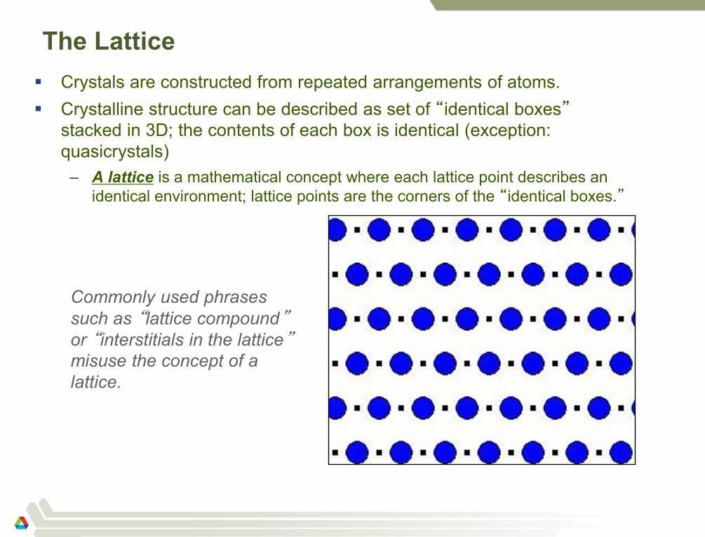
Crystals are constructed from repeated arrangements of atoms.
Crystalline structure can be described as set of “identical boxes” stacked in 3D; the contents of each box is identical (exception:
quasicrystals)
– A lattice is a mathematical concept where each lattice point describes an
identical environment; lattice points are the corners of the “identical boxes.”
6
Commonly used phrases
such as “lattice compound” or “interstitials in the lattice” misuse the concept of a
lattice.
Lattice planes
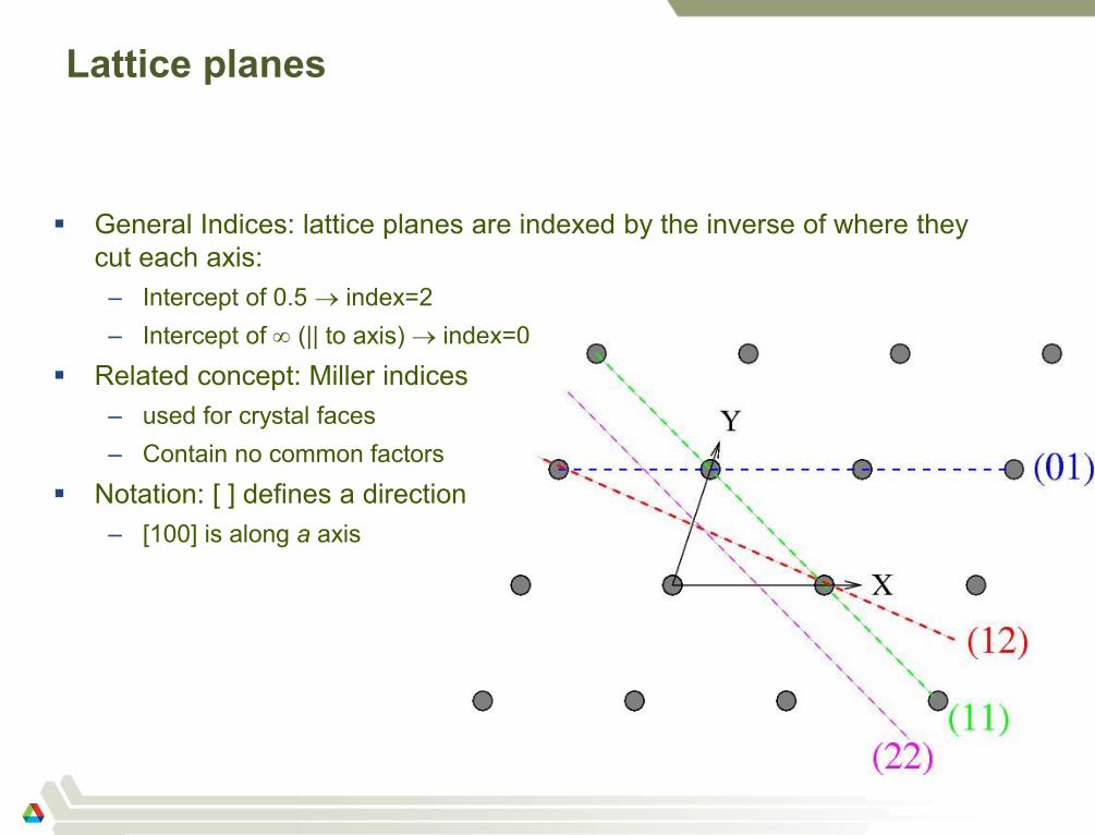
General Indices: lattice planes are indexed by the inverse of where they
cut each axis:
– Intercept of 0.5 index=2
– Intercept of (|| to axis) index=0
Related concept: Miller indices
– used for crystal faces
– Contain no common factors
Notation: [ ] defines a direction
– [100] is along a axis
7

Single Crystal Diffraction
8

Diffraction from single crystals
Diffraction occurs when the reciprocal lattice planes of a crystal are
aligned at an angle with respect to the beam and the wavelength of an
incident beam satisfies:
– n 2 d sin (or better, 4 sin / Q) [Bragg’s Law]
– d = 1/|d*| = 1/|ha* + kb* + lc*|
9
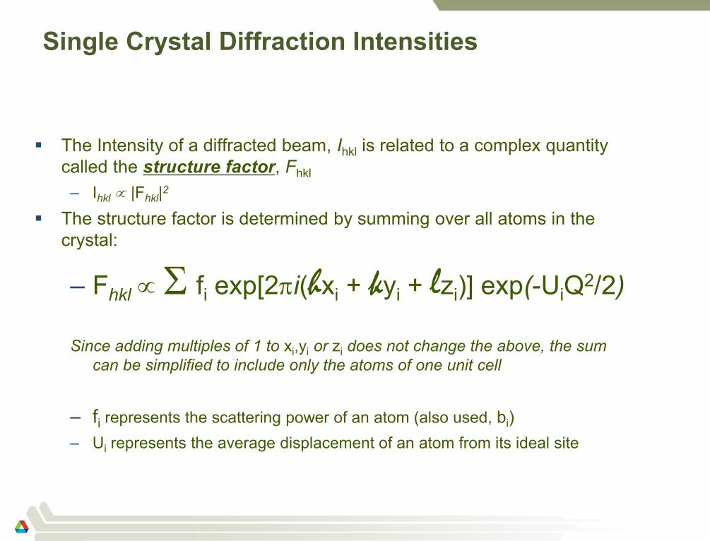
Single Crystal Diffraction Intensities
The Intensity of a diffracted beam, Ihkl is related to a complex quantity
called the structure factor, Fhkl
– Ihkl |Fhkl|2
The structure factor is determined by summing over all atoms in the
crystal:
– Fhkl fi exp[2i(hxi + kyi + lzi)] exp(-UiQ2/2)
Since adding multiples of 1 to xi,yi or zi does not change the above, the sum
can be simplified to include only the atoms of one unit cell
– fi represents the scattering power of an atom (also used, bi)
– Ui represents the average displacement of an atom from its ideal site
10

Powder Diffraction
11
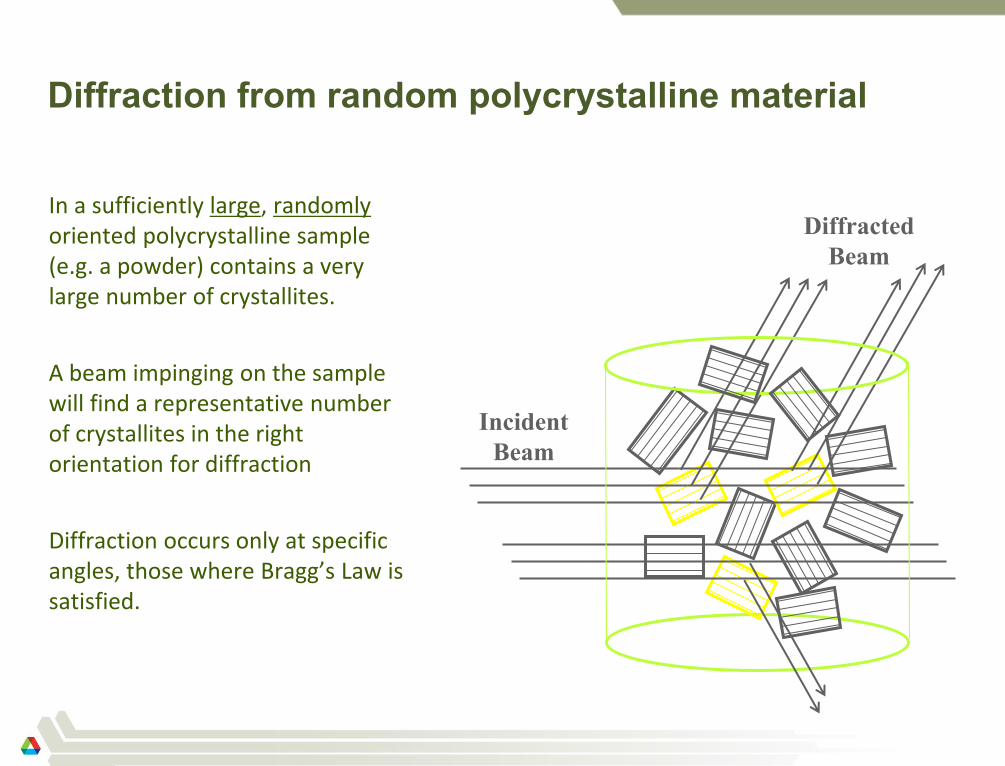
Diffraction from random polycrystalline material
In a sufficiently large, randomly oriented polycrystalline sample (e.g. a powder) contains a very large number of crystallites.
A beam impinging on the sample will find a representative number of crystallites in the right orientation for diffraction
Diffraction occurs only at specific angles, those where Bragg’s Law is satisfied.
12
Incident
Beam
Diffracted
Beam
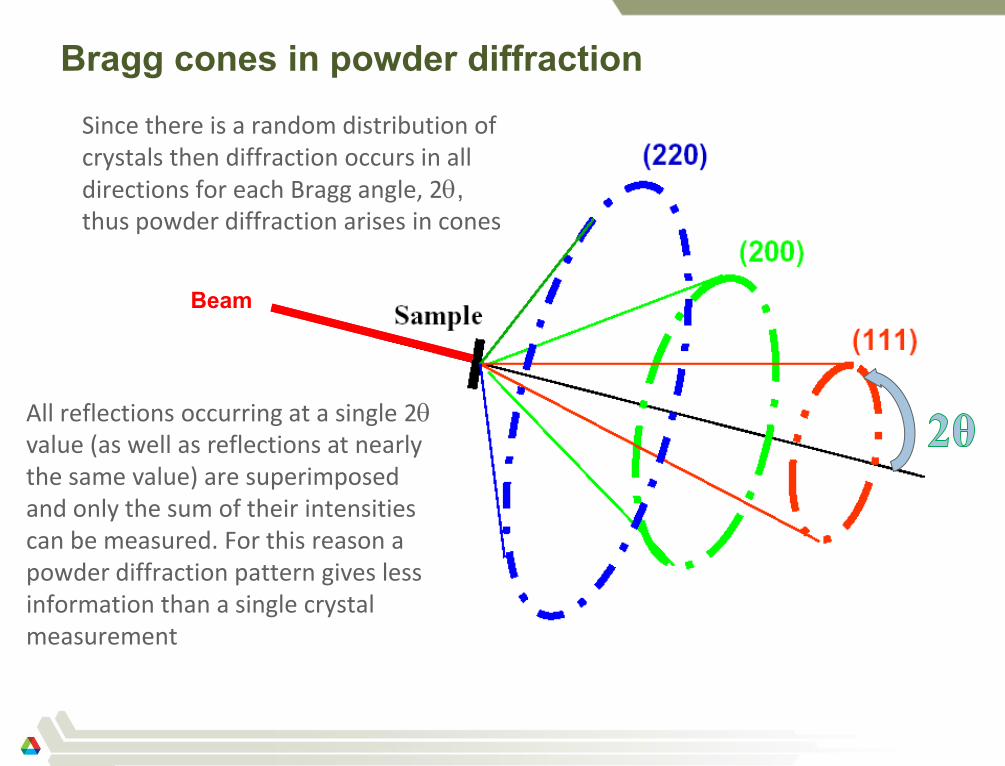
Bragg cones in powder diffraction
13
Beam
All reflections occurring at a single 2 value (as well as reflections at nearly the same value) are superimposed and only the sum of their intensities can be measured. For this reason a powder diffraction pattern gives less information than a single crystal measurement
Since there is a random distribution of crystals then diffraction occurs in all directions for each Bragg angle, 2, thus powder diffraction arises in cones
Diffraction of X-rays versus Neutrons
14
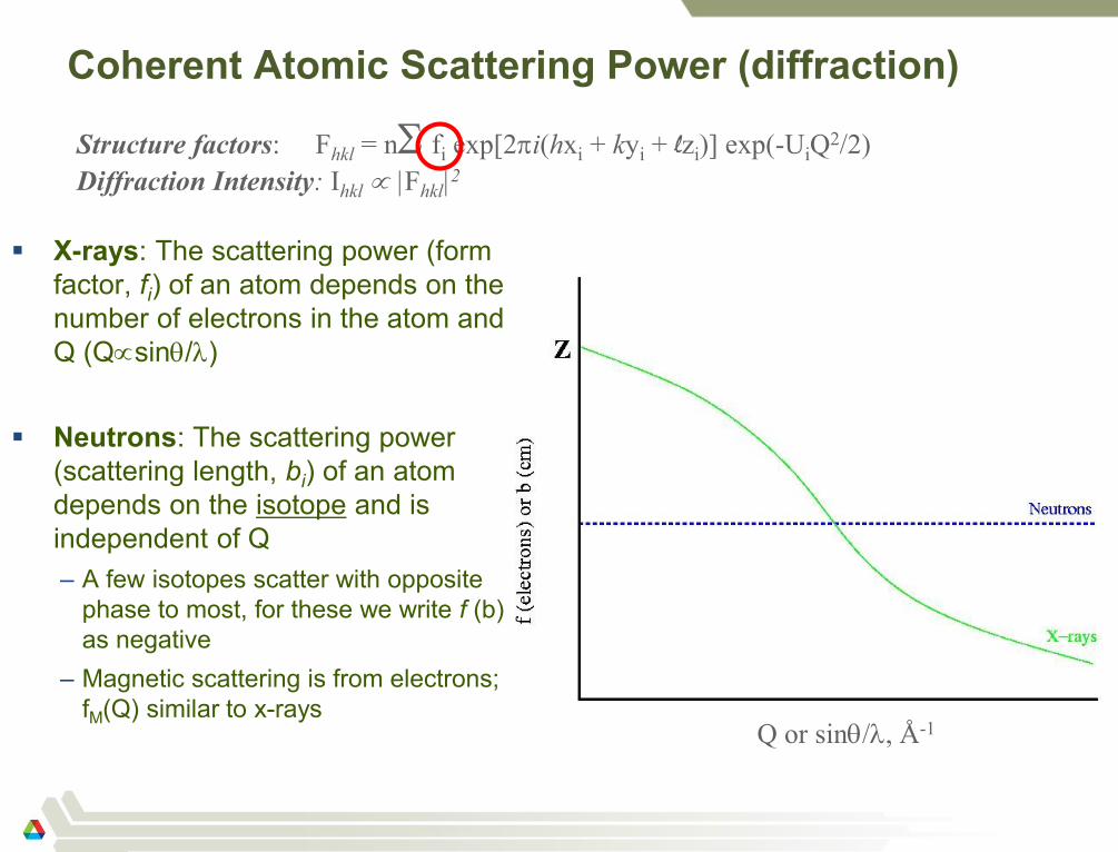
Coherent Atomic Scattering Power (diffraction)
X-rays: The scattering power (form
factor, fi) of an atom depends on the
number of electrons in the atom and
Q (Qsin/)
Neutrons: The scattering power
(scattering length, bi) of an atom
depends on the isotope and is
independent of Q
– A few isotopes scatter with opposite
phase to most, for these we write f (b)
as negative
– Magnetic scattering is from electrons;
fM(Q) similar to x-rays
15
Q or sin/, Å-1
Structure factors: Fhkl = n fi exp[2i(hxi + kyi + lzi)] exp(-UiQ2/2)
Diffraction Intensity: Ihkl |Fhkl|2
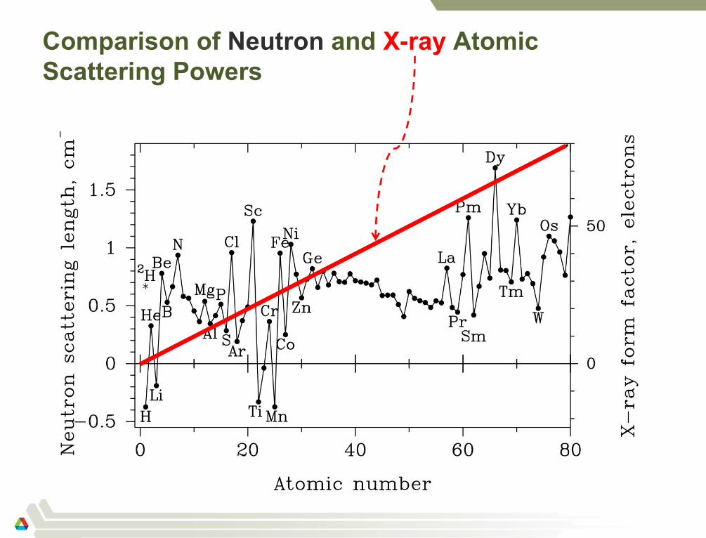
Comparison of Neutron and X-ray Atomic
Scattering Powers
16
17
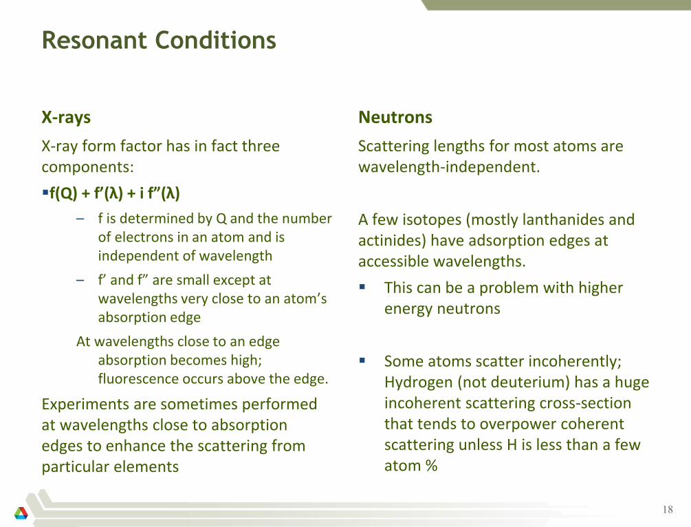
Resonant Conditions
X-rays
X-ray form factor has in fact three components:
f(Q) + f’(λ) + i f”(λ)
– f is determined by Q and the number of electrons in an atom and is independent of wavelength
– f’ and f” are small except at wavelengths very close to an atom’s absorption edge
At wavelengths close to an edge absorption becomes high; fluorescence occurs above the edge.
Experiments are sometimes performed at wavelengths close to absorption edges to enhance the scattering from particular elements
Neutrons
Scattering lengths for most atoms are wavelength-independent.
A few isotopes (mostly lanthanides and actinides) have adsorption edges at accessible wavelengths.
This can be a problem with higher energy neutrons
Some atoms scatter incoherently; Hydrogen (not deuterium) has a huge incoherent scattering cross-section that tends to overpower coherent scattering unless H is less than a few atom %
18

Types of Powder Diffraction
Measurements
19
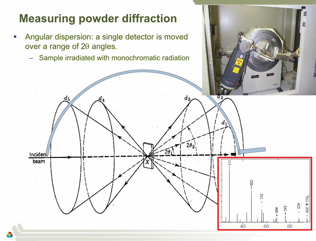
Measuring powder diffraction
Angular dispersion: a single detector is moved
over a range of 2 angles.
– Sample irradiated with monochromatic radiation
20
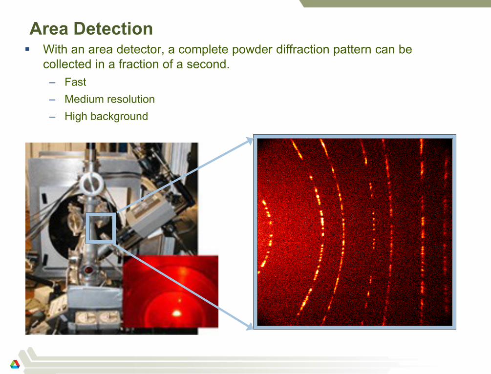
Area Detection With an area detector, a complete powder diffraction pattern can be
collected in a fraction of a second.
– Fast
– Medium resolution
– High background
21
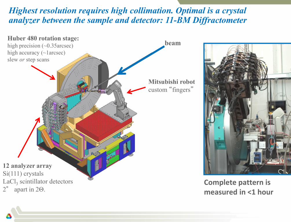
Highest resolution requires high collimation. Optimal is a crystal analyzer between the sample and detector: 11-BM Diffractometer
22
beam Huber 480 rotation stage: high precision (~0.35arcsec)
high accuracy (~1arcsec)
slew or step scans
12 analyzer array
Si(111) crystals
LaCl3 scintillator detectors
2° apart in 2Θ.
Mitsubishi robot
custom “fingers”
Complete pattern is measured in <1 hour
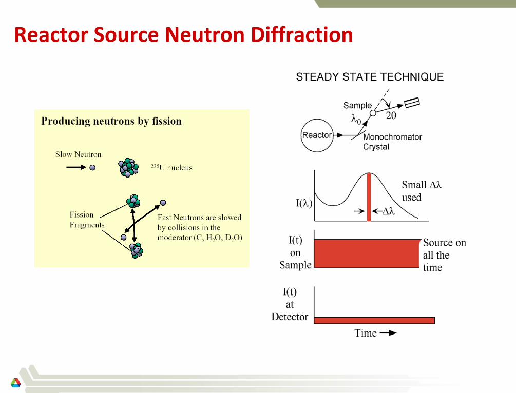
Reactor Source Neutron Diffraction
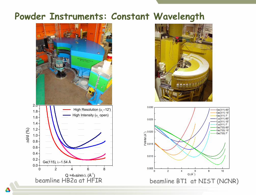
Powder Instruments: Constant Wavelength
beamline HB2a at HFIR
0 2 4 6 80.0
0.2
0.4
0.6
0.8
1.0
1.2
1.4
1.6
1.8
2.0
Ge(115)1.54 Å
Q =4sin (Å-1)
d/d
(%
)
High Resolution (12')
High Intensity (open)
beamline BT1 at NIST (NCNR)
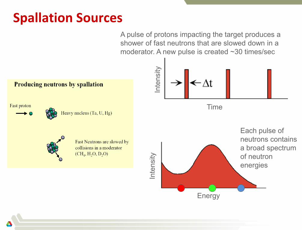
Spallation Sources
Each pulse of
neutrons contains
a broad spectrum
of neutron
energies
Energy
Inte
nsity
Inte
nsity
Time
A pulse of protons impacting the target produces a
shower of fast neutrons that are slowed down in a
moderator. A new pulse is created ~30 times/sec
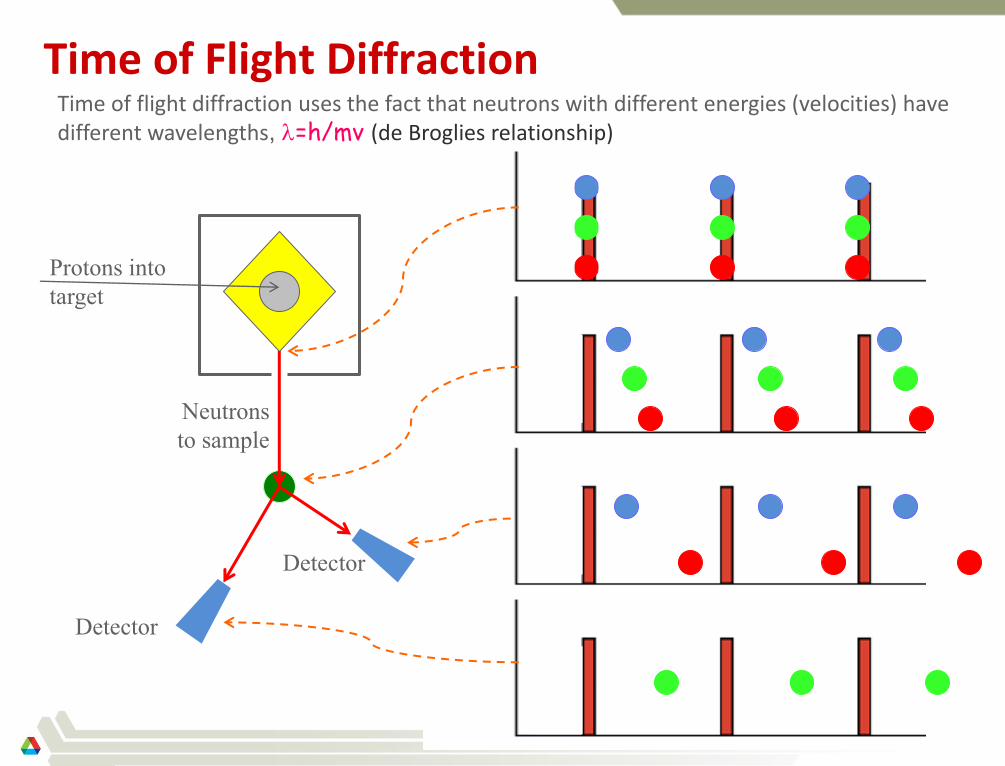
Time of Flight Diffraction
Protons into
target
Neutrons
to sample
Time of flight diffraction uses the fact that neutrons with different energies (velocities) have different wavelengths, =h/mv (de Broglies relationship)
Detector
Detector
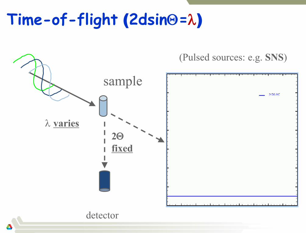
Time-of-flight (2dsin=)
2
fixed
sample
detector
varies
(Pulsed sources: e.g. SNS)
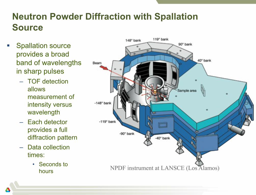
Neutron Powder Diffraction with Spallation
Source
Spallation source
provides a broad
band of wavelengths
in sharp pulses
– TOF detection
allows
measurement of
intensity versus
wavelength
– Each detector
provides a full
diffraction pattern
– Data collection
times:
• Seconds to
hours
28
NPDF instrument at LANSCE (Los Alamos)
Understanding Materials Effects in
Powder Diffraction
29
Materials effects on Powder Diffraction
Peak broadening:
Crystallite size:
– What happens when crystals become small?
Residual Stress (Strain)
– What happens if matrix effects do not allow crystallites to equilibrate lattice
parameters?
30
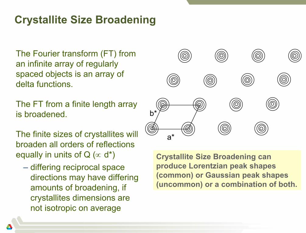
a*
b*
Crystallite Size Broadening can
produce Lorentzian peak shapes
(common) or Gaussian peak shapes
(uncommon) or a combination of both.
Crystallite Size Broadening
The Fourier transform (FT) from
an infinite array of regularly
spaced objects is an array of
delta functions.
The FT from a finite length array
is broadened.
The finite sizes of crystallites will
broaden all orders of reflections
equally in units of Q ( d*)
– differing reciprocal space
directions may have differing
amounts of broadening, if
crystallites dimensions are
not isotropic on average

d*=constant
GSAS fits crystallite broadening
with two profile terms:
• LX -> Lorentzian
• GP -> Gaussian
Relation between avg. size (p) and
GSAS terms:
K 1 (Scherrer constant, related to
crystal shape)
p =18000Kl
pLX
p =18000Kl
p GP
Crystallite Size Broadening
32
See GSAS Manual, pp 158-167.
a*
b*
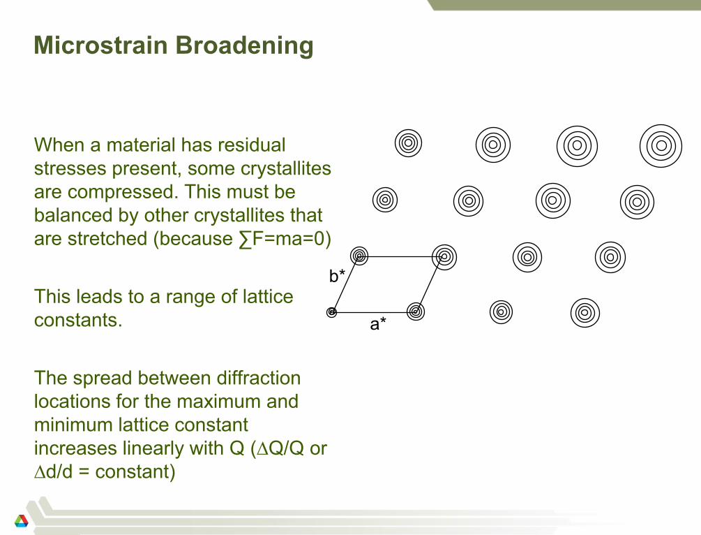
Microstrain Broadening
When a material has residual
stresses present, some crystallites
are compressed. This must be
balanced by other crystallites that
are stretched (because ∑F=ma=0)
This leads to a range of lattice
constants.
The spread between diffraction
locations for the maximum and
minimum lattice constant
increases linearly with Q (∆Q/Q or
∆d/d = constant)
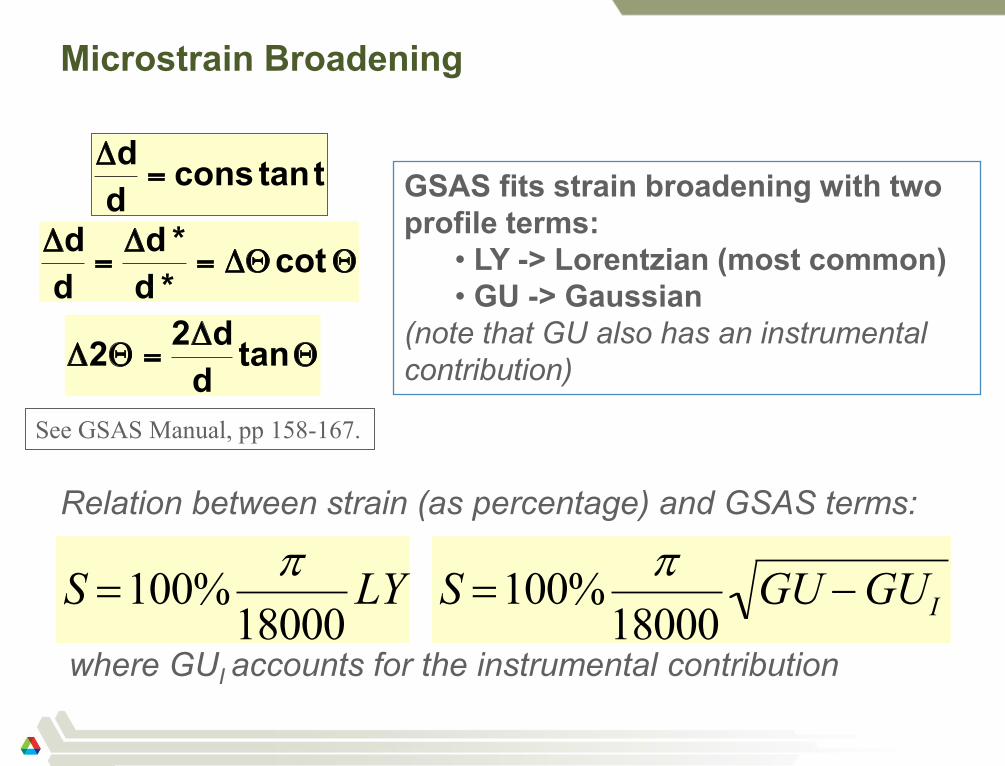
S =100%p
18000LY
S =100%p
18000GU -GUI
Microstrain Broadening
34
GSAS fits strain broadening with two
profile terms:
• LY -> Lorentzian (most common)
• GU -> Gaussian
(note that GU also has an instrumental
contribution)
Relation between strain (as percentage) and GSAS terms:
where GUI accounts for the instrumental contribution
See GSAS Manual, pp 158-167.
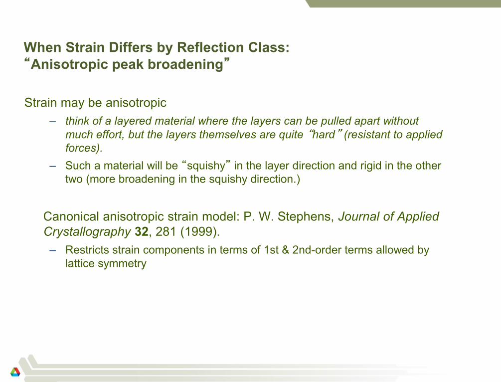
When Strain Differs by Reflection Class:
“Anisotropic peak broadening”
Strain may be anisotropic
– think of a layered material where the layers can be pulled apart without
much effort, but the layers themselves are quite “hard” (resistant to applied
forces).
– Such a material will be “squishy” in the layer direction and rigid in the other
two (more broadening in the squishy direction.)
Canonical anisotropic strain model: P. W. Stephens, Journal of Applied
Crystallography 32, 281 (1999).
– Restricts strain components in terms of 1st & 2nd-order terms allowed by
lattice symmetry
35
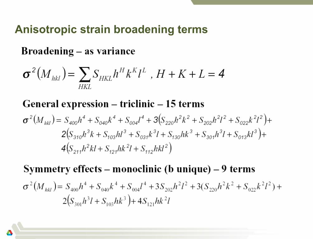
Anisotropic strain broadening terms
36
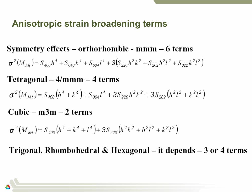
Anisotropic strain broadening terms
37
Fitting of Powder Diffraction Data
(Rietveld Analysis)
38
Why did Crystallography Revolutionize Science?
1. Crystallography was the first scientific technique that provided direct
information about molecular structure
– Early work was intuitive: structures assigned based on patterns and
symmetry (some results predate X-rays!)
2. X-ray and neutron diffraction observations can be modeled very
accurately directly when the molecular structure is known
3. Diffraction can provide a very large number of independent observations
– probability of finding an incorrect structure model that is both plausible and is
in good agreement with the diffraction observations is very small (but not
zero!)
4. Computer-assisted least-squares optimization allows structural models
to be improved, limited only by the quality of the data
5. Statistical and brute-force techniques overcomes the incomplete nature
of diffraction observations (direct methods vs. “the phase problem”).
100+ years later, no other technique offers as much
power for learning about molecular structure!
39
Fitting crystallographic data -- what is it all about?
We perform an experiment:
– Get lots of intensity and position measurements in a diffraction
measurement: what do they tell us?
Obtain an unit cell that fits the diffraction positions (indexing)
“Solve the structure”: determine an approximate model to match the
intensities
Add/modify the structure for completeness & chemical sense
Optimize the structure (model) to obtain the best fit to the observed data
– This is usually done with Gauss-Newton least-squares fitting
– Parameters to be fit are structural and may account for other experimental
effects
Least Squares gives us a Hessian matrix; inverse is variance-covariance
matrix which gives uncertainties in the parameters
40
Crystallography from powder diffraction: before
Rietveld
How did crystallographers use powder diffraction data?
Avoided powder diffraction
Manually integrate intensities
– discard peaks with overlapped reflections
Or
– rewrote single-crystal software to refine using sums of overlapped reflections
Simulation of powder diffraction data was commonly done
Qualitative reasoning: similarities in patterns implied similar structures
Visual comparison between computed and observed structure verifies
approximate model
Fits, where accurate (& precise) models were rarely obtained
Error propagation was difficult to do correctly (but not impossible)
41
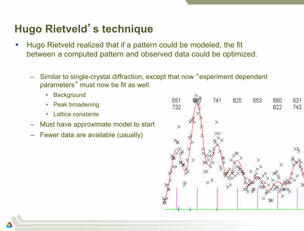
Hugo Rietveld’s technique
Hugo Rietveld realized that if a pattern could be modeled, the fit
between a computed pattern and observed data could be optimized.
– Similar to single-crystal diffraction, except that now “experiment dependent
parameters” must now be fit as well.
• Background
• Peak broadening
• Lattice constants
– Must have approximate model to start
– Fewer data are available (usually)
42
Calculation of Powder Diffraction: Graphical
Example
43
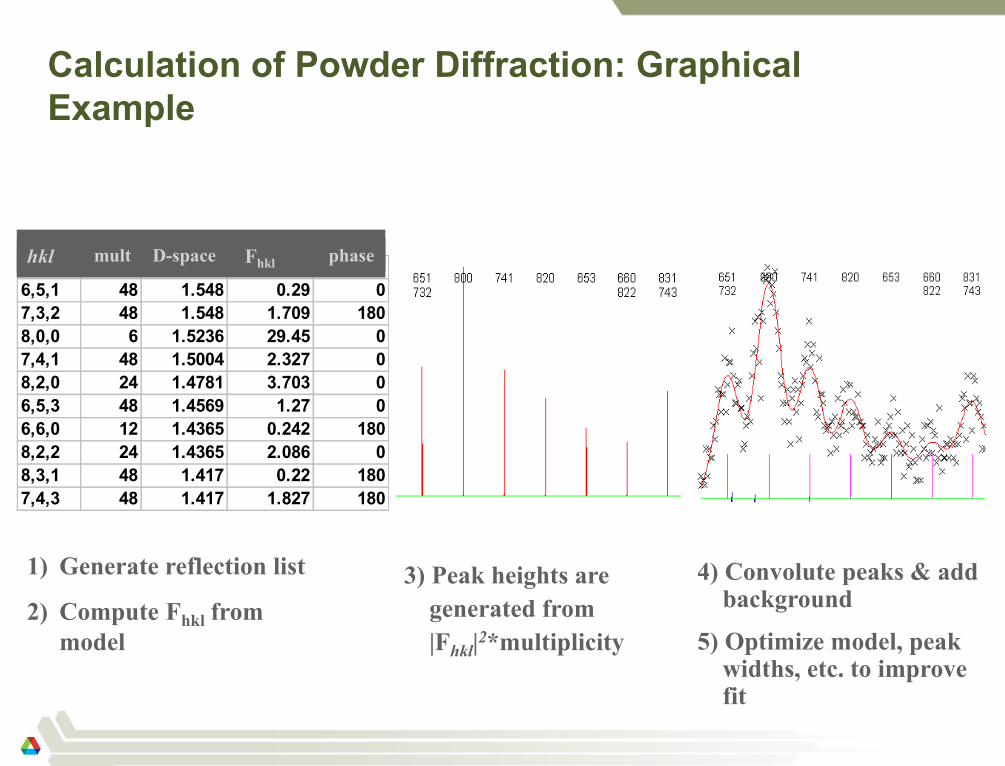
hkl mult d-space Fobs phase
6,5,1 48 1.548 0.29 0
7,3,2 48 1.548 1.709 180
8,0,0 6 1.5236 29.45 0
7,4,1 48 1.5004 2.327 0
8,2,0 24 1.4781 3.703 0
6,5,3 48 1.4569 1.27 0
6,6,0 12 1.4365 0.242 180
8,2,2 24 1.4365 2.086 0
8,3,1 48 1.417 0.22 180
7,4,3 48 1.417 1.827 180
1) Generate reflection list
2) Compute Fhkl from
model
3) Peak heights are
generated from
|Fhkl|2*multiplicity
4) Convolute peaks & add background
5) Optimize model, peak widths, etc. to improve fit
Fhkl phase D-space mult hkl
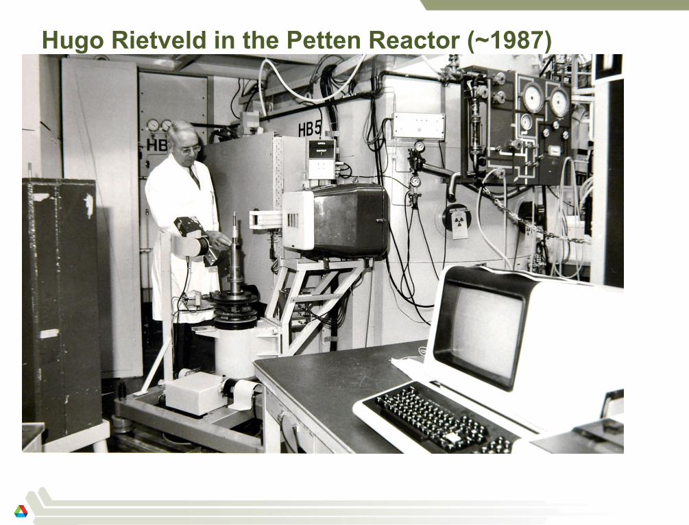
Hugo Rietveld in the Petten Reactor (~1987)
44
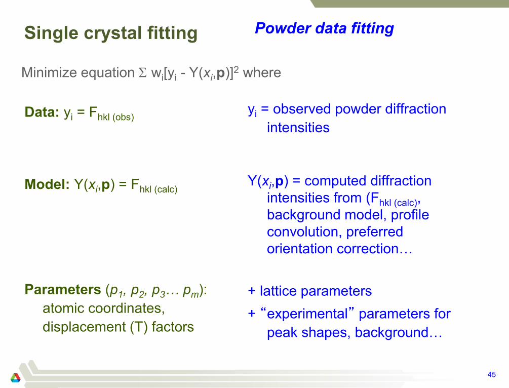
Single crystal fitting
Data: yi = Fhkl (obs)
Model: Y(xi,p) = Fhkl (calc)
Parameters (p1, p2, p3… pm):
atomic coordinates,
displacement (T) factors
yi = observed powder diffraction
intensities
Y(xi,p) = computed diffraction
intensities from (Fhkl (calc),
background model, profile
convolution, preferred
orientation correction…
+ lattice parameters
+ “experimental” parameters for
peak shapes, background…
45
Powder data fitting
Minimize equation wi[yi - Y(xi,p)]2 where
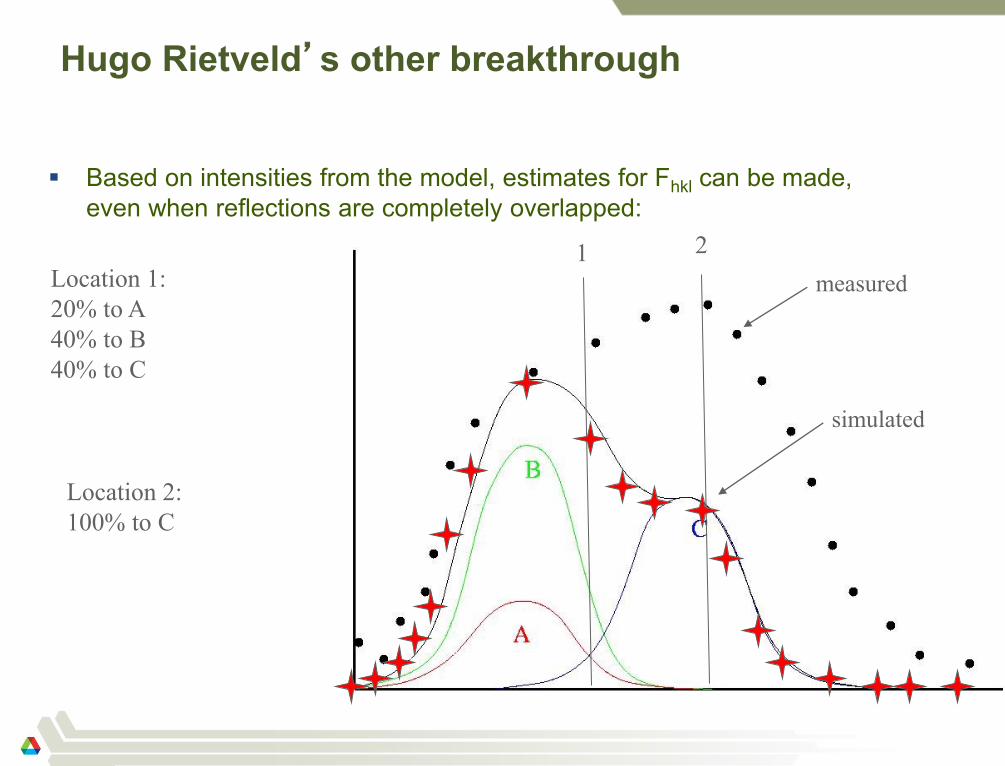
Hugo Rietveld’s other breakthrough
Based on intensities from the model, estimates for Fhkl can be made,
even when reflections are completely overlapped:
46
1 Location 1:
20% to A
40% to B
40% to C
2
Location 2:
100% to C
measured
simulated
Rietveld Applications
Crystallographic structure determination
Quantify amounts of crystalline phases
– (Amorphous content possible indirectly)
Engineering properties
– Residual stress/Crystallite sizes
– Preferred orientation
Lattice constant determination
47
What sort of data are needed for Rietveld Analysis?
Must be possible to fit peak shapes
Q range and resolution demands dictated by structural complexity
Data from lab instruments should be used with caution for structure
determination
Neutron data are usually necessary for occupancy determination
48
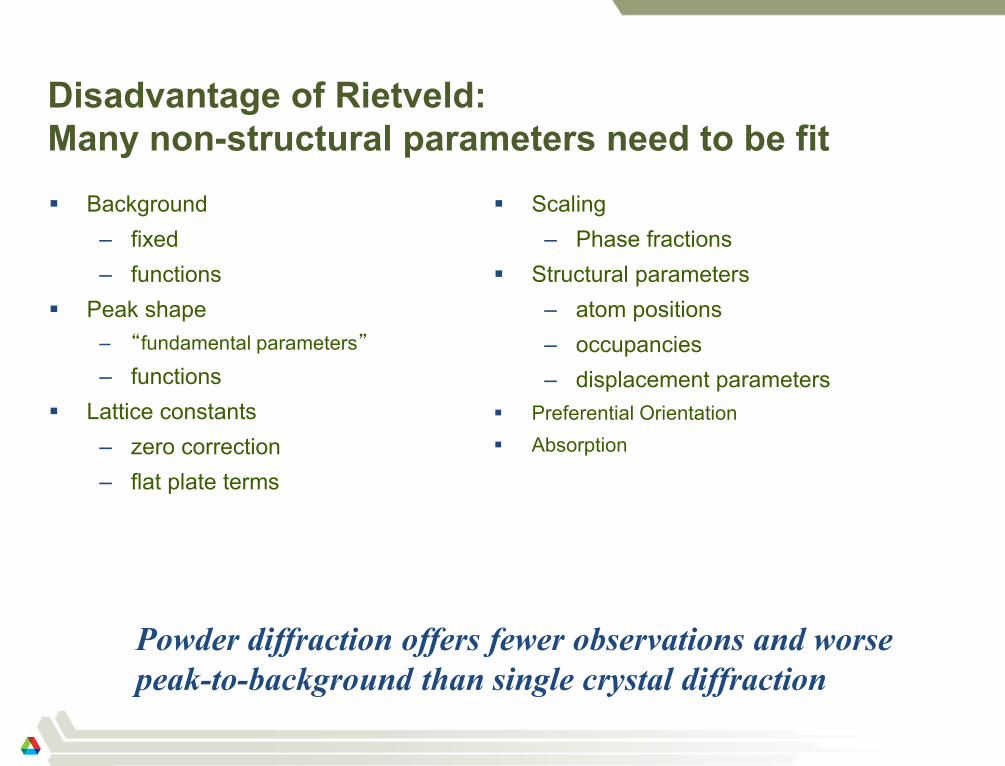
Disadvantage of Rietveld:
Many non-structural parameters need to be fit
Background
– fixed
– functions
Peak shape
– “fundamental parameters”
– functions
Lattice constants
– zero correction
– flat plate terms
Scaling
– Phase fractions
Structural parameters
– atom positions
– occupancies
– displacement parameters
Preferential Orientation
Absorption
49
Powder diffraction offers fewer observations and worse
peak-to-background than single crystal diffraction
Limitations of Rietveld
Rietveld can only discern parameters that have effects on the
powder diffraction pattern
– Cannot separate some effects ever
• Absolute configuration
• Magnetic moment directions unless they break symmetry
If two parameters have approximately the same effect on the
powder diffraction pattern, they correlate and they cannot be
differentiated (e.g. occupancies & displacement parameters)
50
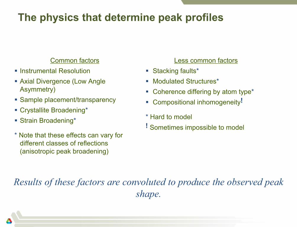
The physics that determine peak profiles
Common factors
Instrumental Resolution
Axial Divergence (Low Angle
Asymmetry)
Sample placement/transparency
Crystallite Broadening*
Strain Broadening*
* Note that these effects can vary for
different classes of reflections
(anisotropic peak broadening)
Less common factors
Stacking faults*
Modulated Structures*
Coherence differing by atom type*
Compositional inhomogeneity!
* Hard to model
! Sometimes impossible to model
51
Results of these factors are convoluted to produce the observed peak
shape.
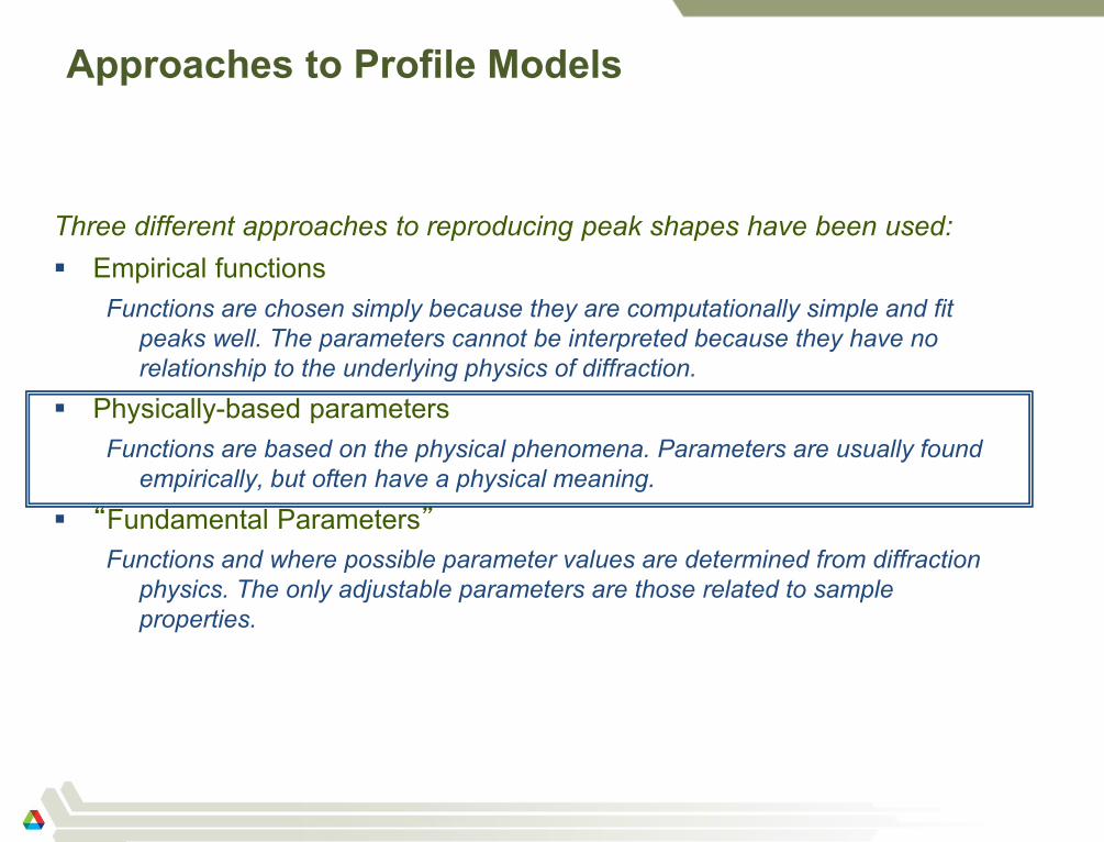
Approaches to Profile Models
Three different approaches to reproducing peak shapes have been used:
Empirical functions
Functions are chosen simply because they are computationally simple and fit
peaks well. The parameters cannot be interpreted because they have no
relationship to the underlying physics of diffraction.
Physically-based parameters
Functions are based on the physical phenomena. Parameters are usually found
empirically, but often have a physical meaning.
“Fundamental Parameters”
Functions and where possible parameter values are determined from diffraction
physics. The only adjustable parameters are those related to sample
properties.
52
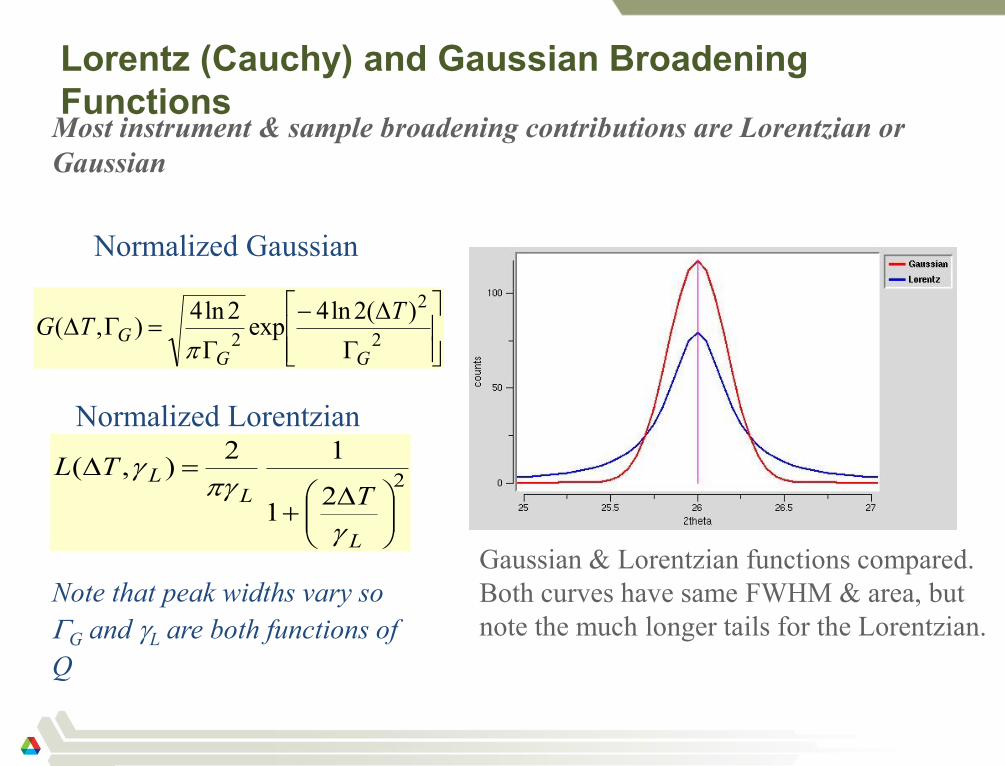
Lorentz (Cauchy) and Gaussian Broadening
Functions
úúû
ù
êêë
é
G
D-
G=GD
2
2
2
)(2ln4exp
2ln4),(
GG
G
TTG
p
53
22
1
12),(
÷÷ø
öççè
æ D+
=D
L
LL
TTL
g
pgg
Most instrument & sample broadening contributions are Lorentzian or
Gaussian
Normalized Gaussian
Normalized Lorentzian
Gaussian & Lorentzian functions compared.
Both curves have same FWHM & area, but
note the much longer tails for the Lorentzian.
Note that peak widths vary so
G and L are both functions of
Q
Voigt vs. Pseudo-Voigt
A Gaussian convoluted with a Lorentzian function is a Voigt function,
however the Voigt is slow to compute and the derivatives are messy.
Few Rietveld programs implement a Voigt.
The “pseudo-Voigt” is the weighted sum of a Gaussian & Lorentzian
function – approximation is normally pretty good
Fractions of each function depend on the relative widths of each [see mixing
factor () in GSAS manual, =0 is Gaussian, =1 is Lorentzian]
54
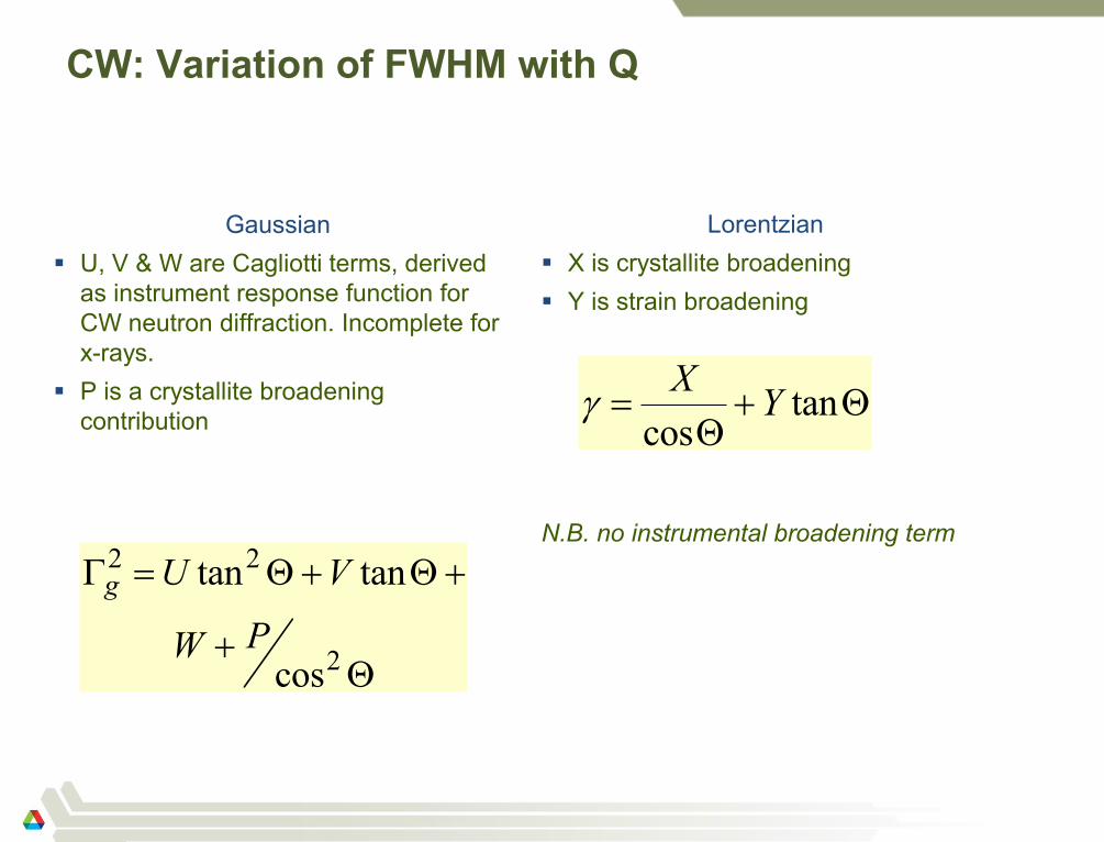
CW: Variation of FWHM with Q
Gaussian
U, V & W are Cagliotti terms, derived
as instrument response function for
CW neutron diffraction. Incomplete for
x-rays.
P is a crystallite broadening
contribution
Lorentzian
X is crystallite broadening
Y is strain broadening
N.B. no instrumental broadening term
55
Q+
+Q+Q=G
2
22
cos
tantan
PW
VUg
Q+Q
= tancos
YX
g
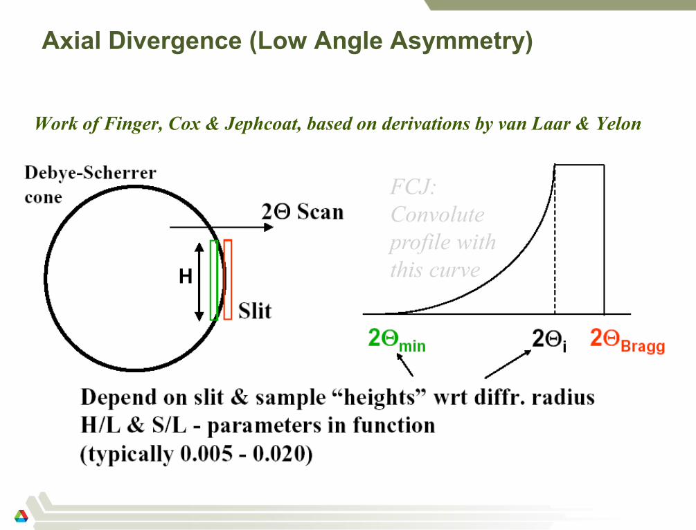
Axial Divergence (Low Angle Asymmetry)
Work of Finger, Cox & Jephcoat, based on derivations by van Laar & Yelon
56
FCJ:
Convolute
profile with
this curve

F-C-J: Example
The Finger-Cox-Jephcoat correctly models the effective shift of the peak
due to axial divergence.
Note: the “competition,”
the split Pearson VII
(empirical), does not
model this effect at all!
57

Sample Displacement & Transparency
In Bragg-Brentano geometry, samples are ideally placed exactly at
rotation axis and all diffraction occurs from sample surface (highly
absorbing sample). Neither is commonly true.
Peak centers are shifted by
– Sample Displacement (SHFT), Ss
– Sample transparency (TRNS), Ts
These corrections correlate very highly with the zero correction for 2,
ZERO. Do not refine this too.
Parallel-Beam instruments (neutron or synchrotron) are very tolerant of
displacement and transparency. Never refine SHFT or TRNS, but do
refine ZERO (correction to 2).
58
Q+Q+D=D 2sincos' ss TSTT
36000
sRSntdisplaceme
p-=
seff
RTpm
9000-=
R is diffractometer radius

Prerequisites for Powder Diffraction
Crystallography Before you try analyzing powder diffraction data you should understand
the following concepts
59
The Unit Cell
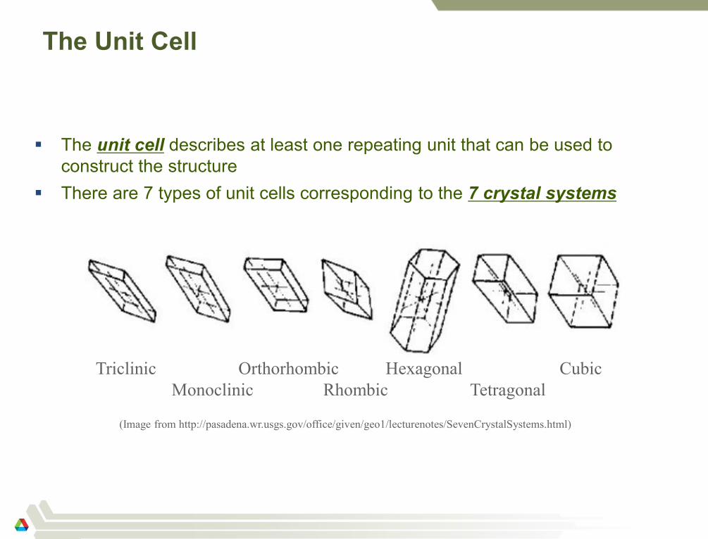
The unit cell describes at least one repeating unit that can be used to
construct the structure
There are 7 types of unit cells corresponding to the 7 crystal systems
60
Triclinic Orthorhombic Hexagonal Cubic
Monoclinic Rhombic Tetragonal
(Image from http://pasadena.wr.usgs.gov/office/given/geo1/lecturenotes/SevenCrystalSystems.html)
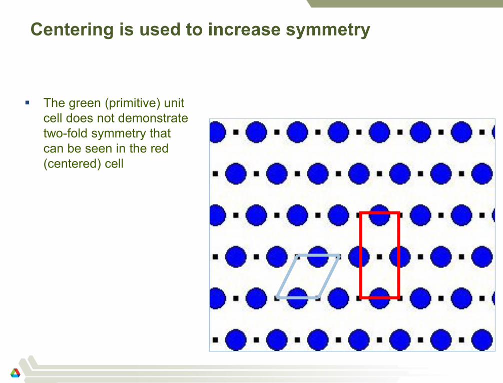
Centering is used to increase symmetry
The green (primitive) unit
cell does not demonstrate
two-fold symmetry that
can be seen in the red
(centered) cell
61

Lattice Types
Centering causes lattice
points to be placed inside
units cells (body center,
face centers) giving rise the
14 Bravais lattices (1848)
62
(Figure from http://www.chemsoc.org/exemplarchem/entries/2003/bristol_cook/latticetypes.htm)
Have non-perpendicular
axes: (non-orthogonal
coordinate systems) {
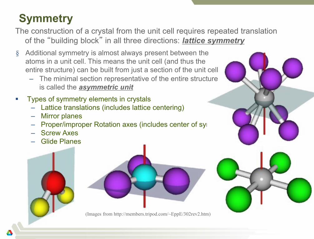
Symmetry
Types of symmetry elements in crystals
– Lattice translations (includes lattice centering)
– Mirror planes
– Proper/improper Rotation axes (includes center of symmetry)
– Screw Axes
– Glide Planes
63
(Images from http://members.tripod.com/~EppE/302rev2.htm)
The construction of a crystal from the unit cell requires repeated translation
of the “building block” in all three directions: lattice symmetry
§ Additional symmetry is almost always present between the
atoms in a unit cell. This means the unit cell (and thus the
entire structure) can be built from just a section of the unit cell
– The minimal section representative of the entire structure
is called the asymmetric unit
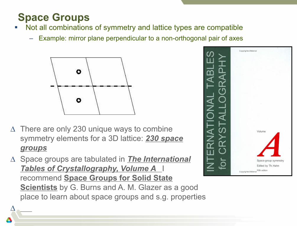
Space Groups Not all combinations of symmetry and lattice types are compatible
– Example: mirror plane perpendicular to a non-orthogonal pair of axes
64
∆ There are only 230 unique ways to combine
symmetry elements for a 3D lattice: 230 space
groups
∆ Space groups are tabulated in The International
Tables of Crystallography, Volume A�I
recommend Space Groups for Solid State
Scientists by G. Burns and A. M. Glazer as a good
place to learn about space groups and s.g. properties
∆ ��
Fractional coordinates
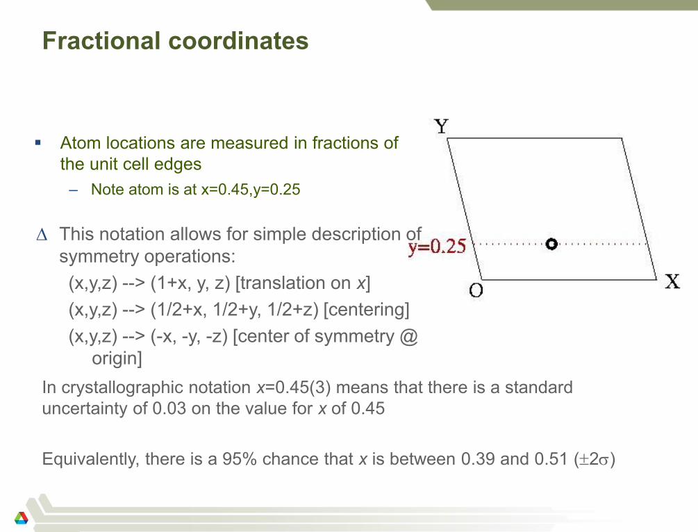
Atom locations are measured in fractions of
the unit cell edges
– Note atom is at x=0.45,y=0.25
65
∆ This notation allows for simple description of
symmetry operations:
(x,y,z) --> (1+x, y, z) [translation on x]
(x,y,z) --> (1/2+x, 1/2+y, 1/2+z) [centering]
(x,y,z) --> (-x, -y, -z) [center of symmetry @
origin]
In crystallographic notation x=0.45(3) means that there is a standard
uncertainty of 0.03 on the value for x of 0.45
Equivalently, there is a 95% chance that x is between 0.39 and 0.51 (2)
Reciprocal Lattice
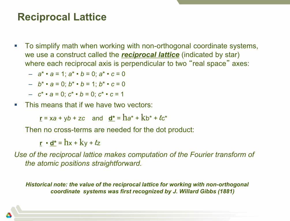
To simplify math when working with non-orthogonal coordinate systems,
we use a construct called the reciprocal lattice (indicated by star)
where each reciprocal axis is perpendicular to two “real space” axes:
– a* • a = 1; a* • b = 0; a* • c = 0
– b* • a = 0; b* • b = 1; b* • c = 0
– c* • a = 0; c* • b = 0; c* • c = 1
This means that if we have two vectors:
r = xa + yb + zc and d* = ha* + kb* + lc*
Then no cross-terms are needed for the dot product:
r • d* = hx + ky + lz
Use of the reciprocal lattice makes computation of the Fourier transform of
the atomic positions straightforward.
Historical note: the value of the reciprocal lattice for working with non-orthogonal
coordinate systems was first recognized by J. Willard Gibbs (1881)
66