a three‐frequency dynamic factor model for nowcasting ... · we are extremely thankful to kevin...

Bank of Canada staff discussion papers are completed staff research studies on a wide variety of subjects relevant to central bank policy, produced independently from the Bank’s Governing Council. This research may support or challenge prevailing policy orthodoxy. Therefore, the views expressed in this paper are solely those of the authors and may differ from official Bank of Canada views. No responsibility for them should be attributed to the Bank.

www.bank-banque-canada.ca

Staff Discussion Paper/Document d’analyse du personnel 2017-8

A Three-Frequency Dynamic Factor Model for Nowcasting Canadian Provincial GDP Growth

by Tony Chernis, Calista Cheung and Gabriella Velasco

2

Bank of Canada Staff Discussion Paper 2017-8

June 2017

A Three-Frequency Dynamic Factor Model for Nowcasting Canadian Provincial GDP Growth

by

Tony Chernis, Calista Cheung and Gabriella Velasco

Canadian Economic Analysis Department

Bank of Canada Ottawa, Ontario, Canada K1A 0G9

[email protected] [email protected] [email protected]

ISSN 1914-0568 © 2017 Bank of Canada

mailto:[email protected]



i

Acknowledgements

We are extremely thankful to Kevin MacLean and Daniel Friedland for excellent research assistance. We would also like to thank seminar participants at the Bank of Canada, as well as Rodrigo Sekkel, Daniel de Munnik and Laurent Martin for their helpful comments. The views expressed in this paper are solely those of the authors.

ii

Abstract

This paper estimates a three-frequency dynamic factor model for nowcasting Canadian provincial gross domestic product (GDP). Canadian provincial GDP at market prices is released by Statistics Canada on an annual basis only, with a significant lag (11 months). This necessitates a mixed-frequency approach that can process timely monthly data, the quarterly national accounts and the annual target variable. The model is estimated on a wide set of provincial, national and international data. We assess the extent to which these indicators can be used to nowcast annual provincial GDP in a pseudo real-time setting and construct indicators of unobserved monthly GDP for each province that can be used to assess the state of regional economies. The monthly activity indicators fit the data well in-sample, are able to track business-cycle turning points across the provinces, and showcase the significant regional heterogeneity that characterizes a large diverse country like Canada. They also provide more timely indications of business-cycle turning points and are able to pick up shorter periods of economic contraction that would not be observed in the annual average. In a pseudo real-time exercise, we find the model outperforms simple benchmarks and is competitive with more sophisticated mixed-frequency approaches such as MIDAS models.

Bank topics: Business fluctuations and cycles; Econometric and statistical methods; Regional economic developments JEL codes: C53, E32, E37, R11

Résumé

Nous estimons un modèle factoriel dynamique reposant sur des données de triple fréquence que nous appliquons à la prévision du produit intérieur brut (PIB) des provinces canadiennes pour la période en cours. Statistique Canada publie le PIB aux prix du marché des provinces canadiennes chaque année, mais avec un décalage non négligeable de onze mois. Ce retard impose de recourir à une méthode qui combine plusieurs fréquences afin de réussir à traiter des données mensuelles plus à jour, les comptes nationaux trimestriels et des données annuelles sur la variable ciblée. Notre modèle est estimé à partir d’un vaste ensemble de statistiques provinciales, nationales et internationales. Nous évaluons l’utilité de ces indicateurs dans la prévision de l’évolution annuelle du PIB des provinces pour la période en cours dans un environnement où les données sont disponibles en temps quasi réel. Nous construisons également des indicateurs de l’évolution mensuelle non observée du PIB de chaque province, qui peuvent servir à évaluer la situation des économies régionales. Ces indicateurs de l’activité mensuelle présentent une bonne adéquation avec les données sur échantillon, retracent les points de retournement du cycle économique dans les provinces, et illustrent bien la forte

iii

hétérogénéité régionale caractéristique d’un pays aussi grand et divers que le Canada. Les indicateurs fournissent aussi des informations plus à jour sur les points de retournement du cycle économique et peuvent déceler de courtes périodes de contraction de l’activité que ne permettent pas d’observer les mesures moyennes annuelles. Dans un environnement où les données sont disponibles en temps quasi réel, notre modèle soutient la comparaison avec des méthodes à fréquence mixte plus sophistiquées, par exemple avec les modèles d’échantillonnage de données de fréquence mixte (MIDAS).

Sujets : Cycles et fluctuations économiques ; Méthodes économétriques et statistiques ; Évolution économique régionale Codes JEL : C53, E32, E37, R11

4

1. IntroductionIn general, conducting economic policy—and specifically monetary policy—requires an

assessment of the state of the economy in real time. Understanding the economy’s current state is a

challenging task that becomes even more difficult when macroeconomic indicators are released with

substantial delays. For example, estimates of Canadian gross domestic product (GDP) are released two

months after the end of the reference quarter. Policy institutions typically deal with these issues using a

mix of simple forecasting models and judgment to predict the near future, current state and recent past

of the economy.

In a geographically diverse country like Canada, tracking regional economic conditions can be

critical to properly assess the state of the broader business cycle and forming economic projections.1

However, assessing provincial economic activity is difficult as few comprehensive indicators are released

in a timely fashion. While a large set of activity indicators are released for the provinces at a monthly

frequency2 and in a more timely manner, they are often less comprehensive than the national‐level

statistics. Furthermore, official data for the most important and comprehensive indicator, real GDP, are

available for the provinces and territories only at an annual frequency and with a significant lag.3 The

expenditure‐based measure of real GDP is released 11 months after the end of the reference year, while

estimates of by‐industry GDP at basic prices are released five months after the end of the reference

year. These data limitations obscure high‐frequency movements in provincial GDP, and limit the series’

usefulness.

Examining the regional dimensions of economic fluctuations can reveal useful insights into the

impact, spillover effects, and adjustment process for various shocks. A number of studies have shown

that regional heterogeneity in a country’s industrial structure can lead to differing responses across

jurisdictions to external shocks and changes in business cycles (DeSerres and Lalonde 1994; Beine and

Coulombe 2003). An example is Owyang, Piger and Wall (2005), who found that US states with higher

shares of employment in mining and construction as well as manufacturing have tended to experience

deeper‐than‐average recessions. Similarly, for Canada Salem (2003) found that provinces that relied

more heavily on cyclical industries such as manufacturing—like Ontario and Quebec—experienced larger

contractions during the 1990–92 recession. Finally, regional disparities may also matter for the efficacy

of monetary policy. For example, Carlino and DeFina (1998) give evidence from the United States that

the transmission of monetary policy is asymmetric across regions. And as argued by Fratantoni and

Schuh (2003), how the economy responds to a monetary tightening depends on which regions are

growing fastest, and how interest‐rate‐sensitive those regions are based on their industrial structure.

Needless to say, understanding regional dynamics matters for economic policy.

1 In some cases, exploiting provincial data and inter‐regional dependencies can help produce superior forecasts of national GDP growth, as demonstrated by Demers and Dupuis (2005). 2 For example, the Labour Force Survey is available on a monthly basis a few weeks after the end of the reference month. 3 The Ontario Ministry of Finance and Institut de la Statistique du Québec produce quarterly estimates with less of a lag, which are subsequently benchmarked to the official Statistics Canada figures.

5

One way to monitor regional dynamics is by building coincident indicators. Economists have a

long history of building coincident indicators, going at least as far back as Burns and Mitchell’s (1946)

time at the National Bureau of Economic Research (NBER). This continued with the Organisation for

Economic Co‐operation and Development (OECD) and the Conference Board of Canada, which have long

published composite activity indicators. More sophisticated approaches have been developed using

dynamic factor models, such as Stock and Watson (1989, 1999, 2002), Mariano and Murasawa (2003),

Aruoba, Diebold and Scotti (2009), Aruoba and Diebold (2010), Forni et al. (2000) and Matheson (2011).

Similarly, Evans (2005) estimates high‐frequency GDP but does not use a factor model approach.

Methods have been applied on a regional level by Crone and Clayton‐Matthews (2005) to create

coincident indicators for the 50 US states using the methodology from Stock and Watson (1989). More

recently, the field of nowcasting has emerged (Giannone, Reichlin and Small 2008), which studies

estimating GDP in real time. This broad literature explicitly addresses the unique set of challenges

presented by the flow of macroeconomic data in real time. This includes mixed frequencies, unbalanced

panels of data (ragged edges), large sets of data, and data revisions. Today there are a large number of

papers using different methodologies, with dynamic factor models featured prominently. Camacho and

Perez‐Quiros (2010) offer an excellent example.

Until recently, there have been very few papers that focus on nowcasting in Canada (Galbraith

and Tkacz 2017; Binette and Chang 2013; Bragoli and Modugno 2016; Chernis and Sekkel 2017).

However, there has been little work on nowcasting provincial GDP. The closest application we are aware

of is Kopoin, Moran and Paré (2013), who study the role of national and international data for

forecasting GDP in Ontario and Quebec using a factor model and targeted predictors.

Instead, efforts have been directed towards estimating provincial GDP at higher frequencies.

Quebec and Ontario have quarterly estimates of expenditure‐based GDP, produced respectively by the

Institut de la Statistique du Québec and the Ontario Ministry of Finance, while only Quebec has a

monthly measure of industry‐based GDP at basic prices. It is important to note that these measures are

estimates of quarterly GDP, and are subsequently benchmarked to the Statistics Canada annual data

upon their release. Other institutions have attempted to fill this data gap by constructing their own

independent measures of regional economic activity. For example, the Conference Board of Canada

publishes estimates of real GDP for the provinces and territories on a quarterly basis.4 The National Bank

also publishes a monthly Index of Provincial Economic Momentum (IPEM) that summarizes changes in

seven monthly indicators based on the methodology used by the US Conference Board for its leading

4 The Conference Board of Canada produces quarterly estimates of real GDP at basic prices and GDP at market prices for all the provinces. These estimates are benchmarked to the annual GDP measures, with quarterly values derived from a highly intricate process projecting each component of GDP onto a monthly indicator, under the overarching constraint of adding up to the quarterly national GDP. As argued by Lamy and Sabourin (2001), the measures may not be reliable reference series given their low correlation with series such as employment and real retail sales compared with their national counterparts.

6

indicator of the US economy.5 A similar technique is used by Alberta Treasury Board and Finance for its

Alberta Activity Index.6 The federal Department of Finance Canada used a similar approach to develop

quarterly coincident indexes of economic activity for each Canadian province and territory (Lamy and

Sabourin 2001), as well as leading indicators (Cawthray, Gaudreault and Lamy 2002), although these

indexes were not released to the public. These latter two approaches draw on a very small subset of the

data that are available by province, leaving potentially valuable information unused.

The main contribution of this paper is the building of a nowcasting model that targets the

annual provincial real GDP data from Statistics Canada using a combination of monthly, quarterly and

annual data. We do this by developing a dynamic factor model (DFM) for each of the Canadian

provinces. The DFM approach elegantly handles the typical problems faced by an analyst: mixed

frequencies, an unbalanced panel (the ragged edges), the relatively large data set available, and the

existence of noisy leading indicators such as GDP at basic prices. In addition, the model produces a

measure of unobserved monthly GDP that can be used to assess the state of the economy at a much

higher frequency than the target data. We examine the behaviour of the monthly GDP indicator, and

study the nowcasting performance of the model in a pseudo real‐time forecasting exercise.

First, the model fits the data well in‐sample. The monthly activity indicators are able to track

recessions and business‐cycle turning points across the provinces. Furthermore, they showcase the

significant regional differences fundamental to a large diverse country like Canada. They also provide

more timely indications of business‐cycle turning points and are able to pick up shorter periods of

economic contraction that would not be observed in the annual average. In a pseudo real‐time exercise,

we find the model outperforms simple benchmarks and is competitive with more sophisticated mixed‐

frequency approaches like MIDAS. In addition, we find that in most cases, data sets using only provincial

data fit the data better7 and are more useful for nowcasting.

The paper is organized as follows: Section 2 describes the data used in our model and Section 3

presents the dynamic factor model approach. Section 4 discusses the results both in‐sample and in the

context of a pseudo real‐time forecasting exercise. Section 5 concludes.

2.DataWhen building a nowcasting model, the choice of variables is a critical step. We select variables

based on the following criteria: (i) they are directly related to the Canadian and provincial economies, (ii)

they are updated frequently (monthly or quarterly), and (iii) they have minimal publication delay. To

help us meet these criteria, we choose variables that are followed by the market and reported on

5 The IPEM for each province is a weighted average of the normalized symmetric growth rates of the following seven monthly indicators: employment, housing starts, retail sales, wholesale trade, manufacturing sales, the value of non‐residential building permits, and average weekly earnings. 6 See http://www.finance.alberta.ca/aboutalberta/archive‐alberta‐activity‐index.html for the methodology. 7 This is slightly different from Kopoin, Moran and Paré (2013), who find that international and national data improve forecasts of GDP growth at shorter horizons. However, they find little improvement over provincial data sets at horizons of a year or more—precisely the horizons we are interested in.

7

Statistics Canada's official release bulletin The Daily. Furthermore, we use a medium‐sized data set

because recent papers (e.g., Alvarez, Camacho and Perez‐Quiros 2016; Luciani 2014; Bańbura and

Modugno 2014) that use a similar DFM approach show that medium‐sized data sets (i.e., with 10–30

variables) perform equally as well as models with larger data sets of over 100 variables. Furthermore,

Boivin and Ng (2006) and Bai and Ng (2008) show that carefully selecting the data can improve the

factor estimates. This results in data sets of approximately 35 variables that include a mix of provincial,

national and international variables, as detailed in Table 1 in the Appendix.

In terms of provincial data, we include around 20 province‐specific indicators from surveys that

include the Labour Force Survey (LFS), Survey of Employment, Payroll and Hours (SEPH), Monthly Survey

of Manufacturers (MSM), retail and wholesale trade surveys, as well as data on building permits,

housing starts, international merchandise trade and Multiple Listing Service (MLS) home prices and

sales. Unfortunately, some of these surveys report only nominal values (international merchandise

trade, MSM, retail and wholesale trade surveys) for provincial series. In addition to these core series, for

some provinces we include additional indicators to capture some of the unique regional characteristics

of the economy. For example, for Alberta, we include the following variables to capture its heavy

dependence on the oil and gas sector: Western Canada Select (WCS) oil prices, Baker‐Hughes drilling rig

counts, and oil and gas extraction by national GDP at basic prices. Similarly, we include the Brent crude

oil price in the data set for Newfoundland and Labrador. For Ontario, we include the quarterly

expenditure‐based GDP estimates produced by the Ontario Ministry of Finance, and for Quebec we

include both the quarterly expenditure‐based GDP and monthly industry‐based GDP measures produced

by the Institut de la Statistique du Québec.8

At the national level, we include around 10 indicators meant to capture the broader Canadian

business cycle. The series we select are real GDP (monthly at basic prices and quarterly at market

prices), international merchandise trade statistics, and national analogues of the provincial data series.

However, instead of the surveys for manufacturing sales, wholesale and retail trade, we opt to use the

corresponding GDP by industry series. This is because, although the data lag is two weeks longer, we can

construct real series over a much longer sample. Finally, we include 5 indicators to capture international

developments, with a focus on Canada’s largest trading partner, the United States. These indicators

include the Chicago Fed National Activity Index (CFNAI), US GDP, the Global Real Activity Indicator for

Canadian Exports (GRACE),9 the Bank of Canada Commodity Price Index (BCPI) and the Canadian

Effective Exchange Rate (CEER).10

There is a notable peculiarity in Canadian macroeconomic data: Canada has GDP indicators with

different release schedules. GDP at basic prices measures production by industry, while GDP at market

prices uses the standard expenditure approach. On a national basis, GDP at basic prices is released on a

monthly basis two months after the reference month, while the expenditure measure is released on a

8 Since these are estimates of the Statistics Canada numbers that are subsequently revised to be consistent with the Statistics Canada benchmark, we do not impose a relationship between them and annual provincial GDP. 9 For more details on this measure, see Binette, Chernis and de Munnik (2017). 10 See Barnett, Charbonneau and Poulin‐Bellisle (2016) for details.

8

quarterly basis with a similar lag. As previously mentioned, GDP for the provinces is available only at

annual frequency, with the basic‐price measure published in May of the following year and the market‐

price measure released in November—11 months after the reference year. This creates challenges for

economic policy; for example, in Alberta it would take until May of 2016 to know the full impact of the

late‐2014 oil price decline on GDP and until November to know any of the expenditure‐side details.

The basic‐price and market‐price GDP series are distinct measures that can occasionally have

quite different growth rates. In theory, the difference lies in the treatment of taxes and subsidies on the

products. While production at basic prices excludes taxes and subsidies, GDP at market prices includes

them. In addition, the two approaches have different measurement methodologies, which can result in

further differences prior to the full reconciliation of the economic accounts.11 This discrepancy can lead

to significant differences in growth rates between the two series—sometimes close to a percentage

point in absolute value in a given year. Nonetheless, GDP at basic prices is a very important predictor of

GDP at market prices because of the earlier timing of its release. Furthermore, the basic‐price GDP

series provide monthly value‐added production details on many industries, which may be especially

helpful for some provinces that represent a large proportion of national production in a specific

industry, such as manufacturing for Ontario or oil and gas extraction for Alberta. However, GDP at

market prices is the traditional expenditure approach and is therefore the focus of analysis.

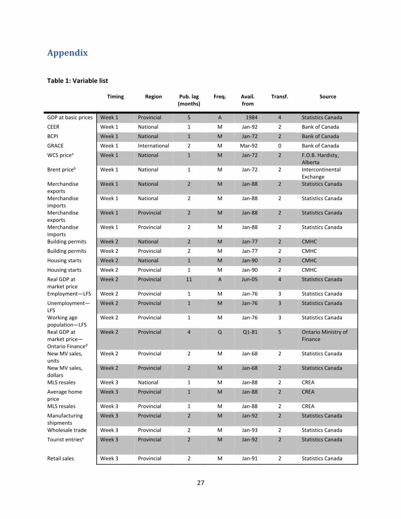
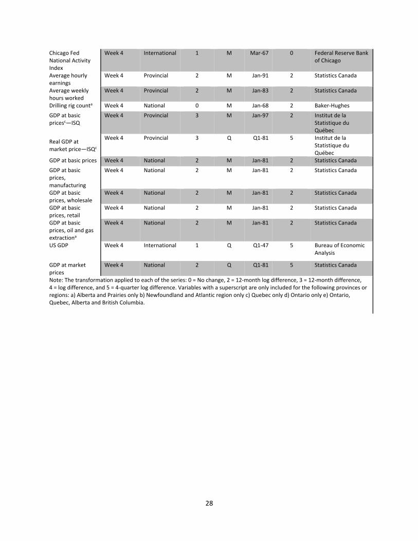
Table 1 in the Appendix shows details of all the series as well as their transformations and release

order. Some series have been rebased or had minor definitional changes, which makes finding series

with sufficient history difficult. In these cases, we splice the most recent series with the corresponding

older series.

3. EconometricFrameworkWe follow the approach proposed by Giannone, Reichlin and Small (2008) with the maximum

likelihood estimation methodology of Bańbura and Modugno (2014), which allows for arbitrary patterns

of missing data. Doz, Giannone and Reichlin (2012) study the asymptotic properties of quasi‐maximum

likelihood estimation for large approximate DFMs. The authors find that the maximum likelihood

estimates of the factors are consistent, as the size of the cross‐section and sample go to infinity along

any path. Furthermore, the estimator is robust to a limited degree of cross‐sectional and serial

correlation of the error terms. This is particularly useful because in large panels, the assumption of no

cross‐correlation could be too restrictive.

First, our model obeys the factor model representation:

ΛF ε , (1)

11 It takes three years for Statistics Canada to produce the Input‐Output tables that reconcile the Canadian macroeconomic accounts.

9

⋯ , (2)

ε , ~ . . . 0,

~ . . . 0,

where is a standardized vector of observables, denotes a vector of r unobserved factors driving the dynamics in the data, and is a vector of idiosyncratic components. In addition, ε , ε , 0 . Λ is the loadings matrix, and , … , are the matrix of coefficients governing the

vector autoregressive process of the factors.

The number of factors estimated in equation 2 is chosen by using Bai and Ng’s (2002)

information criteria modified for use with dynamic factor models (see Modugno, Soybilgen and Yazgan

2016). The number of lags in equation 2 is chosen by Bayesian information criteria (BIC). For details on

the specifications, please see the Appendix.

3.1.Mixed‐frequencyapproachYear‐over‐year quarterly and annual series are incorporated into the model by expressing them

in terms of their partially observed monthly counterparts, which is done through a modification of the

approximation in Mariano and Murasawa (2003). Dahlhaus, Guénette and Vasishtha (2015) and

Giannone, Agrippino and Modugno (2013) show how to apply this to quarterly year‐over‐year variables,

and we extend this technique to annual variables. An example of this technique on an annual basis is

Paredes, Pérez and Perez‐Quiros (2015), who use a quarter‐over‐quarter formulation to forecast annual

government expenditures using quarterly fiscal updates. Annual variables, like GDP ( ), are

expressed as the sum of their unobserved monthly contributions ( ):

⋯

for 12,24, …define 100 log and 100 log . The unobserved

monthly year‐over‐year growth rate, ∆ , is also assumed to follow the same factor model

representation as the monthly variables:

Λ F ε

To link with the observed annual GDP series, we construct a partially observed monthly series:

, 12,24…,

The monthly unobserved year‐over‐year GDP growth can be linked to a partially observed (at the 12th

month of the year) annual year‐over‐year rate using the following:

1

10

1 1 ⋯

1 …

⋯

which results in the annual variables loading equally on the current and lagged values of the unobserved

monthly factor. Similarly, for the quarterly variables, , they can be represented as

where, as before, the quarterly variable loads equally on the current and past values of the unobserved

monthly factor.

The choice of using a year‐over‐year formulation instead of a month‐over‐month approach

makes for a more parsimonious model. As detailed above, the year‐over‐year approach requires relating

12 monthly values to the annual figure, and 3 for a quarterly variable. Using a month‐over‐month

formulation, the number of monthly values increases to 23 and 5, respectively. Furthermore, this

technique is a log approximation and the month‐over‐month formulation on annual basis could

exacerbate any approximation error.

3.2. AdditionalconsiderationsSome modifications must be made to the model to accommodate the GDP at basic prices, which

leads the market prices by six months. Since GDP at basic prices and market prices are distinct measures

but are closely related, we model the basic‐price GDP series as GDP at market prices with some

measurement noise. We use a similar modelling strategy as Camacho and Perez‐Quiros (2010) in their

Euro‐Sting model.12 To be more precise:

ε ,

which results in revising the factor model specification to include these two equations:

ΛF ε ε ,

ΛF ε ,

12 Camacho and Perez‐Quiros are concerned with forecasting the final release so they model the revision patterns between first and final releases as noise, following Evans (2005). While we use a similar strategy, the interpretation is slightly different—we consider the difference between the two measures of GDP as noise.

11

with ε and ε as, respectively, the idiosyncratic component of GDP with variance and an

independent mean zero shock with variance representing the difference between the two measures

of GDP.

For the purposes of this paper, the indicator of underlying growth—the monthly activity

indicator—is simply the common component of growth estimated in equation 1, after excluding the

error term. Or, more formally:

ΛF , (3)

As a consequence of the mixed‐frequency approach, Λ is a (1 x w) vector and F is (w x 1) vector

with w defined as r x 12. This results in being the 12‐month‐over‐12‐month change in GDP, such that

the value observed in December will be annual growth for that year. However, for some applications we

back out the monthly year‐over‐year growth rate. From above, ⋯ are the

contributions to annual growth, so x 12 is the monthly year‐over‐year growth rate for period t.

3.3. ImpactofnewdatareleasesNowcasters are frequently interested in the impact of each new data release on the forecast for

GDP. For example, if incorporating the latest employment data changes the GDP forecast significantly,

we can conclude that there is important “news” content in the employment release. Furthermore, the

nowcasting environment is characterized by a large set of variables that can arrive at a high frequency.

This results in the nowcaster frequently updating the nowcasts to reflect the steady stream of new

information arriving. The DFM framework used in this paper and developed by Giannone, Reichlin and

Small (2008) allows us to quantify this so‐called news. As discussed in Bańbura et al. (2012), by analyzing

the forecast revision, we have a way of quantifying the change in information set and the average

impact of each variable.

Let Ω denote a vintage of data available at time , where refers to the date of a particular

data release. Since data are constantly arriving, Ω expands throughout the nowcast period.

Furthermore, let us denote GDP growth at time as . In this context, we can decompose a new

forecast into two components:

|Ω

|Ω

|I

where I is the subset of the set Ω that is orthogonal to all the elements of Ω . As specified above,

the change in nowcast is due to the unexpected part of the new data release, which is called the news.

The news is useful because what matters in understanding the updating process of the nowcast is not

the release itself but the difference between the release and the previous forecast. Hence, the effect of

the news is given by

12

|Ω |Ω

, , , , , , |Ω∈

where , , are weights obtained from the model estimation and is the set of new variables. The

nowcast revision is a combination of the news associated with the data release for each variable and its

relevancy for the target variable (quantified by its weight , , ). This decomposition allows the

nowcaster to trace forecast revisions back to unexpected movements in individual predictors.

4. ResultsIn this section, we describe the design of the out‐of‐sample forecast exercise, discuss the choice

of data sets and how the model’s performance will be assessed, before finally reporting the results. We

first compare the model’s performance by using the full data set versus a smaller subset of mainly

provincial variables. This is done by examining the in‐sample fit for the provinces and regions, and

comparing the out‐of‐sample root mean square forecast errors (RMSFE) across models. Based on this

assessment, we select the preferred specifications for each province and discuss the results from these

specifications. This includes a discussion of how well the monthly activity indicators track GDP and

behave during important business‐cycle turning points, and of the out‐of‐sample performance relative

to statistical benchmarks. Lastly, we analyze the impact of each data release on the forecasts to

determine which indicators are most important for each province.

4.1.ForecastexercisedesignThe following describes the design of the pseudo real‐time out‐of‐sample exercise used to

assess the model’s forecasting performance. By pseudo we mean that we use the latest available

vintage of data, and not real‐time data sets. While many studies stress the importance of taking into

account data revisions (Croushore and Stark 2002 and 2003; Orphanides 2001), we do not have real‐

time vintages available for all the series. Regardless, using revised data we create vintages of data for

every data release in our sample. This is unlikely to unduly affect the results since factor models are

robust to data revisions, as stressed in Giannone, Reichlin and Small (2008). Using these vintages, we

update our prediction for each new release of data. Table 1 shows the assumed order of data availability

and ragged edge pattern. The model is estimated recursively starting in 1981 and the first out‐of‐sample

forecast is made for 2000. This leaves us with 15 annual data points to assess the performance of our

model. We begin our predictions at the release of provincial GDP at market prices in November for the

previous year. From that point we construct a backcast, nowcast and forecast for annual GDP growth at

every data release, depending on the point in the annual forecast cycle. For example, in November

2000, the annual provincial GDP data for 1999 are released. From that point until the end of the year,

the model creates for each province a GDP growth nowcast for the year 2000 and a forecast for the year

2001. From January 2001, the year 2000 becomes a backcast, the nowcast is for the year 2001, and the

forecast for year 2002. Each of these backcasts, nowcasts and forecasts is revised with every data

release, until the annual provincial GDP data for 2000 are released in November 2001.

13

4.2.ChoiceofdatasetAs discussed earlier, we consider a data set of about 35 variables at the provincial, national and

international levels for estimating the composite activity indicators. As part of a federation sharing a

common currency and government, all provinces will be influenced to some degree by common national

factors such as changes in monetary policy, federal fiscal policy and exchange rates. However, the extent

to which a province’s economy is influenced by national and international variables will vary depending

on its size and linkages with other provinces and countries through trade or movement of people. We

thus consider two estimates of the composite activity indicators using two alternative data sets: (i) a

data set including only province‐specific data13 as well as quarterly national GDP to capture the broader

national business cycle, and (ii) the complete data set that includes all provincial, national and

international variables. These are hereafter referred to as the “provincial‐data‐set model” and the “full‐

data‐set model,” respectively. The preferred specification is selected based on a combination of in‐

sample fit and relative out‐of‐sample performance.

First, we examine the in‐sample fit of the activity measures on an annual basis. This is done by

taking the indicator (from equation 3) on an annual basis and running regressions against the annual

GDP growth series. We also test whether amalgamating some of the smaller provinces into regional

aggregates can produce superior fit: this is done for the Prairies (Alberta, Saskatchewan and Manitoba)

and the Atlantic provinces (Nova Scotia, New Brunswick, Prince Edward Island and Newfoundland and

Labrador).

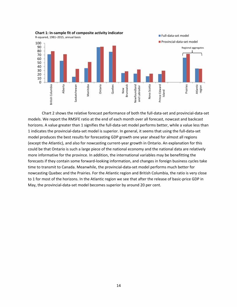
Chart 1 shows the in‐sample fit as measured by the R2 over the sample 1982 to 2015. Overall,

the in‐sample fit is good—most notably, the R2 for Ontario and Quebec is very high around 0.9.14 In the

case of all provinces, the provincial‐data‐set model measures fit the historical data better. This is the

opposite for the Atlantic region, but the difference in fit is small. Furthermore, the Prairies and Atlantic

regions have a better in‐sample fit than their individual components, except for Alberta. Overall,

aggregating the smaller provinces into regions seems to make them more predictable. This is likely

because the smaller provinces are more susceptible to idiosyncratic shocks, such as mine closures or a

new oil platform starting production, and aggregating the regions helps to average some of these out.

For this reason, the following sections focus on five models: Ontario, Quebec, British Columbia, the

Prairies and the Atlantic region. Detailed results are available in the Appendix.

13 Given the importance of the oil sector, the Alberta and Prairies provincial data sets include the WCS oil price series, the Baker‐Hughes drilling rig counts, and the national basic‐price GDP series for oil and gas extraction. Similarly, for Newfoundland and Labrador, we include the Brent crude oil price in the provincial data set. 14 This result is robust to the inclusion of the provincial GDP measures produced by the local Finance ministries.

14

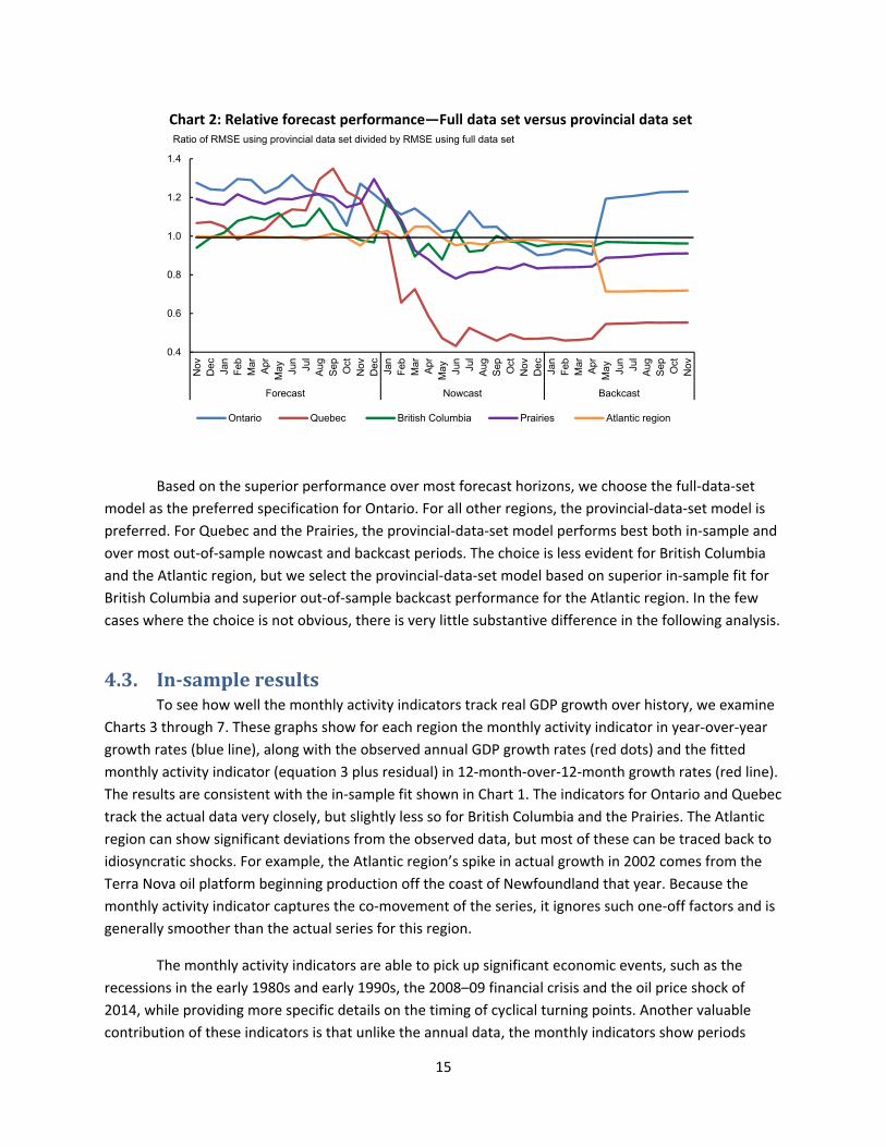
Chart 2 shows the relative forecast performance of both the full‐data‐set and provincial‐data‐set

models. We report the RMSFE ratio at the end of each month over all forecast, nowcast and backcast

horizons. A value greater than 1 signifies the full‐data‐set model performs better, while a value less than

1 indicates the provincial‐data‐set model is superior. In general, it seems that using the full‐data‐set

model produces the best results for forecasting GDP growth one year ahead for almost all regions

(except the Atlantic), and also for nowcasting current‐year growth in Ontario. An explanation for this

could be that Ontario is such a large piece of the national economy and the national data are relatively

more informative for the province. In addition, the international variables may be benefitting the

forecasts if they contain some forward‐looking information, and changes in foreign business cycles take

time to transmit to Canada. Meanwhile, the provincial‐data‐set model performs much better for

nowcasting Quebec and the Prairies. For the Atlantic region and British Columbia, the ratio is very close

to 1 for most of the horizons. In the Atlantic region we see that after the release of basic‐price GDP in

May, the provincial‐data‐set model becomes superior by around 20 per cent.

0102030405060708090

100

British Columbia

Alberta

Saskatchew

an

Man

itoba

Ontario

Queb

ec

New

Brunsw

ick

New

foundland

and Lab

rador

Nova Scotia

Prince Edward

Island

Prairies

Atlan

tic

region

Chart 1: In‐sample fit of composite activity indicator R‐squared, 1981–2015, annual basis Full‐data‐set model

Provincial‐data‐set model

Regional aggregates

15

Based on the superior performance over most forecast horizons, we choose the full‐data‐set

model as the preferred specification for Ontario. For all other regions, the provincial‐data‐set model is

preferred. For Quebec and the Prairies, the provincial‐data‐set model performs best both in‐sample and

over most out‐of‐sample nowcast and backcast periods. The choice is less evident for British Columbia

and the Atlantic region, but we select the provincial‐data‐set model based on superior in‐sample fit for

British Columbia and superior out‐of‐sample backcast performance for the Atlantic region. In the few

cases where the choice is not obvious, there is very little substantive difference in the following analysis.

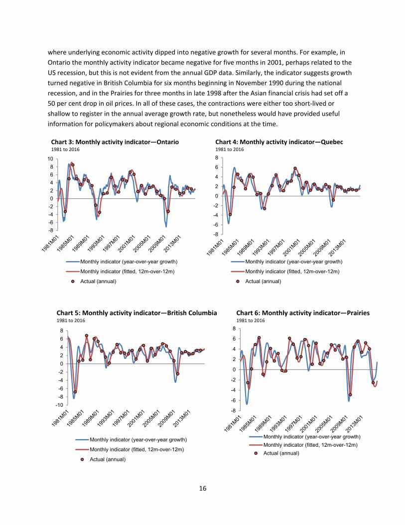
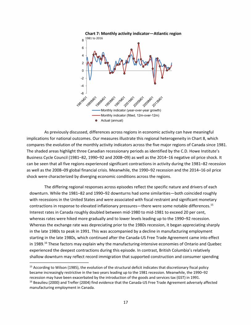
4.3. In‐sampleresultsTo see how well the monthly activity indicators track real GDP growth over history, we examine

Charts 3 through 7. These graphs show for each region the monthly activity indicator in year‐over‐year

growth rates (blue line), along with the observed annual GDP growth rates (red dots) and the fitted

monthly activity indicator (equation 3 plus residual) in 12‐month‐over‐12‐month growth rates (red line).

The results are consistent with the in‐sample fit shown in Chart 1. The indicators for Ontario and Quebec

track the actual data very closely, but slightly less so for British Columbia and the Prairies. The Atlantic

region can show significant deviations from the observed data, but most of these can be traced back to

idiosyncratic shocks. For example, the Atlantic region’s spike in actual growth in 2002 comes from the

Terra Nova oil platform beginning production off the coast of Newfoundland that year. Because the

monthly activity indicator captures the co‐movement of the series, it ignores such one‐off factors and is

generally smoother than the actual series for this region.

The monthly activity indicators are able to pick up significant economic events, such as the

recessions in the early 1980s and early 1990s, the 2008–09 financial crisis and the oil price shock of

2014, while providing more specific details on the timing of cyclical turning points. Another valuable

contribution of these indicators is that unlike the annual data, the monthly indicators show periods

0.4

0.6

0.8

1.0

1.2

1.4

Nov

Dec Jan

Feb

Mar

Apr

May Ju

nJu

lA

ugS

ep Oct

Nov

Dec Jan

Feb

Mar

Apr

May Ju

nJu

lA

ugS

ep Oct

Nov

Dec Jan

Feb

Mar

Apr

May Ju

nJu

lA

ugS

ep Oct

Nov

Forecast Nowcast Backcast

Ontario Quebec British Columbia Prairies Atlantic region

Chart 2: Relative forecast performance—Full data set versus provincial data setRatio of RMSE using provincial data set divided by RMSE using full data set

16

where underlying economic activity dipped into negative growth for several months. For example, in

Ontario the monthly activity indicator became negative for five months in 2001, perhaps related to the

US recession, but this is not evident from the annual GDP data. Similarly, the indicator suggests growth

turned negative in British Columbia for six months beginning in November 1990 during the national

recession, and in the Prairies for three months in late 1998 after the Asian financial crisis had set off a

50 per cent drop in oil prices. In all of these cases, the contractions were either too short‐lived or

shallow to register in the annual average growth rate, but nonetheless would have provided useful

information for policymakers about regional economic conditions at the time.

-8

-6

-4

-2

0

2

4

6

8

10

Chart 3: Monthly activity indicator—Ontario1981 to 2016

Monthly indicator (year-over-year growth)

Monthly indicator (fitted, 12m-over-12m)

Actual (annual)

-8

-6

-4

-2

0

2

4

6

8

Chart 4: Monthly activity indicator—Quebec1981 to 2016



Actual (annual)

-10

-8

-6

-4

-2

0

2

4

6

8



Actual (annual)

Chart 5: Monthly activity indicator—British Columbia 1981 to 2016

-8

-6

-4

-2

0

2

4

6

8



Actual (annual)

Chart 6: Monthly activity indicator—Prairies 1981 to 2016

17

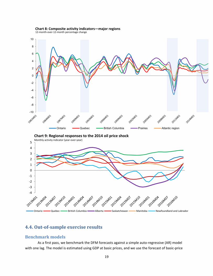
As previously discussed, differences across regions in economic activity can have meaningful

implications for national outcomes. Our measures illustrate this regional heterogeneity in Chart 8, which

compares the evolution of the monthly activity indicators across the five major regions of Canada since 1981.

The shaded areas highlight three Canadian recessionary periods as identified by the C.D. Howe Institute’s

Business Cycle Council (1981–82, 1990–92 and 2008–09) as well as the 2014–16 negative oil price shock. It

can be seen that all five regions experienced significant contractions in activity during the 1981–82 recession

as well as the 2008–09 global financial crisis. Meanwhile, the 1990–92 recession and the 2014–16 oil price

shock were characterized by diverging economic conditions across the regions.

The differing regional responses across episodes reflect the specific nature and drivers of each

downturn. While the 1981–82 and 1990–92 downturns had some similarities—both coincided roughly

with recessions in the United States and were associated with fiscal restraint and significant monetary

contractions in response to elevated inflationary pressures—there were some notable differences.15

Interest rates in Canada roughly doubled between mid‐1980 to mid‐1981 to exceed 20 per cent,

whereas rates were hiked more gradually and to lower levels leading up to the 1990–92 recession.

Whereas the exchange rate was depreciating prior to the 1980s recession, it began appreciating sharply

in the late 1980s to peak in 1991. This was accompanied by a decline in manufacturing employment

starting in the late 1980s, which continued after the Canada‐US Free Trade Agreement came into effect

in 1989.16 These factors may explain why the manufacturing‐intensive economies of Ontario and Quebec

experienced the deepest contractions during this episode. In contrast, British Columbia’s relatively

shallow downturn may reflect record immigration that supported construction and consumer spending 15 According to Wilson (1985), the evolution of the structural deficit indicates that discretionary fiscal policy became increasingly restrictive in the two years leading up to the 1981 recession. Meanwhile, the 1990–92 recession may have been exacerbated by the introduction of the goods and services tax (GST) in 1991. 16 Beaulieu (2000) and Trefler (2004) find evidence that the Canada‐US Free Trade Agreement adversely affected manufacturing employment in Canada.

-6

-4

-2

0

2

4

6

8



Actual (annual)

Chart 7: Monthly activity indicator—Atlantic region 1981 to 2016

18

during this period (Georgopoulos 2009). The Atlantic region appears to experience generally shallower

recessions than the other four regions but also lower average growth during expansionary periods,

which may reflect the relatively large government and non‐durable goods sectors.

More recently, the negative oil price shock appears to have triggered the most severe

contractions in 2015–16 in Alberta, followed by Saskatchewan and Newfoundland and Labrador, the

main oil‐producing regions. This can be seen in Chart 9, which compares the year‐over‐year growth in

the monthly activity index of these provinces with that of the four largest non‐energy‐producing

provinces over recent history. The monthly indicator allows us to see that underlying economic activity

in Alberta responded immediately to the oil price shock, deteriorating in the second half of 2014 when

the steepest price declines occurred, and eventually contracting from early 2015 to late 2016. Although

the economies of the non‐energy‐producing provinces continued to expand during this period, growth

appeared to weaken noticeably in Manitoba and to a lesser extent temporarily in British Columbia and

Ontario, where trade linkages with Alberta are substantial. Meanwhile, the oil price shock had no visible

impact on economic activity in Quebec. By late 2016, growth appeared to be recovering across almost

all provinces, with the exception of Newfoundland and Labrador recovering slightly more slowly.

19

4.4.Out‐of‐sampleexerciseresults

Benchmarkmodels As a first pass, we benchmark the DFM forecasts against a simple auto‐regressive (AR) model

with one lag. The model is estimated using GDP at basic prices, and we use the forecast of basic‐price

-10

-8

-6

-4

-2

0

2

4

6

8

10

Ontario Quebec British Columbia Prairies Atlantic region

Chart 8: Composite activity indicators—major regions12‐month‐over‐12‐month percentage change

‐4

‐3

‐2

‐1

0

1

2

3

4

5

Chart 9: Regional responses to the 2014 oil price shock Monthly activity indicator (year‐over‐year)

Ontario Quebec British Columbia Alberta Saskatchewan Manitoba Newfoundland and Labrador

20

GDP as a forecast for market‐price GDP. We adopt this approach so that we can take into account the

earlier release of GDP at basic prices.

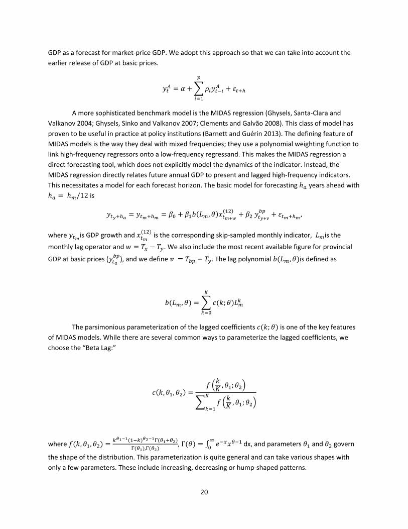
A more sophisticated benchmark model is the MIDAS regression (Ghysels, Santa‐Clara and

Valkanov 2004; Ghysels, Sinko and Valkanov 2007; Clements and Galvão 2008). This class of model has

proven to be useful in practice at policy institutions (Barnett and Guérin 2013). The defining feature of

MIDAS models is the way they deal with mixed frequencies; they use a polynomial weighting function to

link high‐frequency regressors onto a low‐frequency regressand. This makes the MIDAS regression a

direct forecasting tool, which does not explicitly model the dynamics of the indicator. Instead, the

MIDAS regression directly relates future annual GDP to present and lagged high‐frequency indicators.

This necessitates a model for each forecast horizon. The basic model for forecasting years ahead with

/12 is

, ,

where is GDP growth and is the corresponding skip‐sampled monthly indicator, is the

monthly lag operator and . We also include the most recent available figure for provincial

GDP at basic prices ( ), and we define . The lag polynomial , is defined as

, ;

The parsimonious parameterization of the lagged coefficients ; is one of the key features

of MIDAS models. While there are several common ways to parameterize the lagged coefficients, we

choose the “Beta Lag:”

, ,, ;

, ;

where , ,,

, Γ dx, and parameters and govern

the shape of the distribution. This parameterization is quite general and can take various shapes with

only a few parameters. These include increasing, decreasing or hump‐shaped patterns.

21

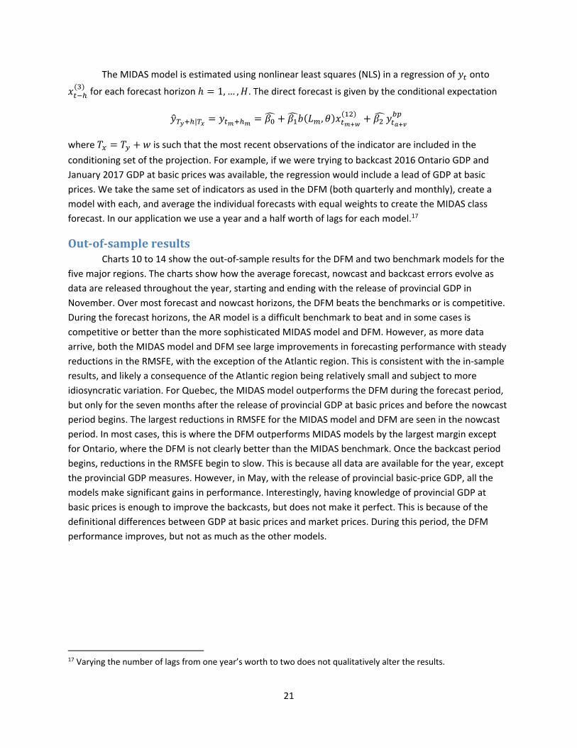
The MIDAS model is estimated using nonlinear least squares (NLS) in a regression of onto

for each forecast horizon 1, … , . The direct forecast is given by the conditional expectation

| ,

where is such that the most recent observations of the indicator are included in the

conditioning set of the projection. For example, if we were trying to backcast 2016 Ontario GDP and

January 2017 GDP at basic prices was available, the regression would include a lead of GDP at basic

prices. We take the same set of indicators as used in the DFM (both quarterly and monthly), create a

model with each, and average the individual forecasts with equal weights to create the MIDAS class

forecast. In our application we use a year and a half worth of lags for each model.17

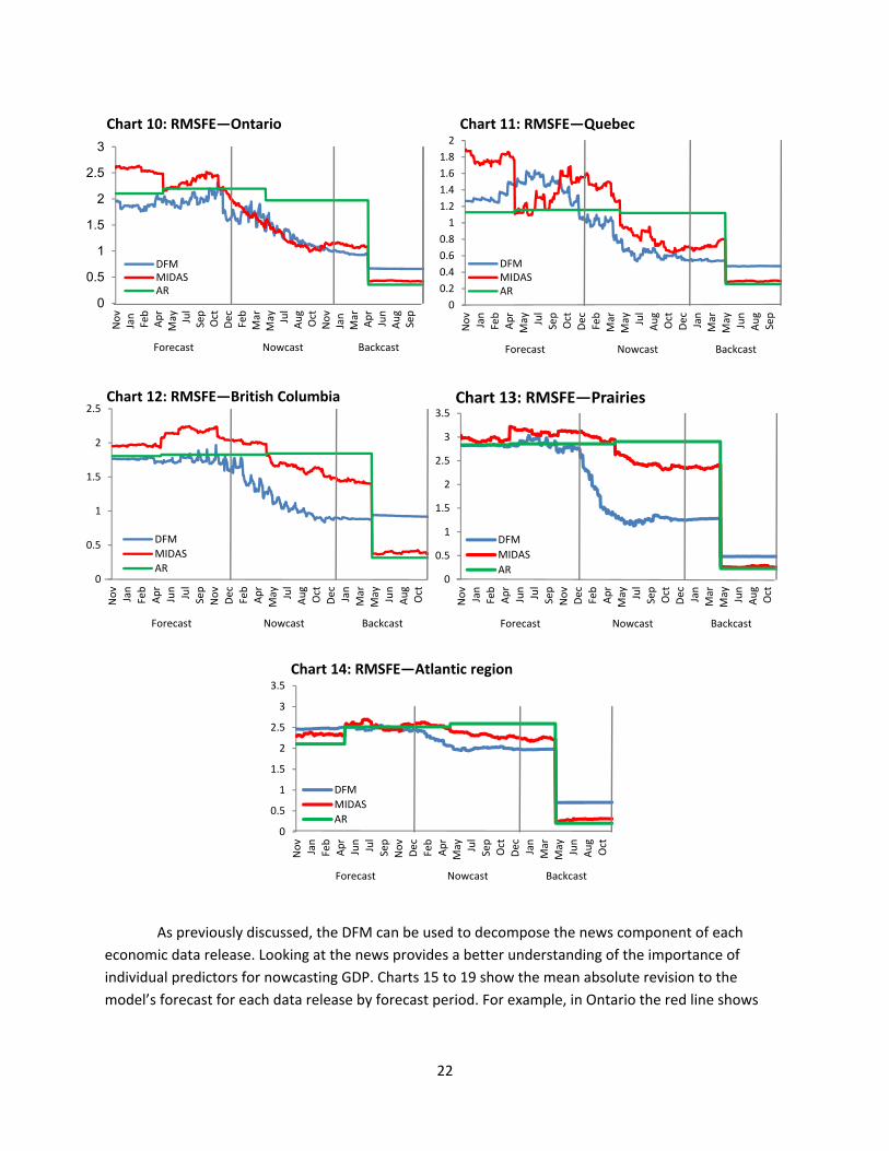
Out‐of‐sampleresultsCharts 10 to 14 show the out‐of‐sample results for the DFM and two benchmark models for the

five major regions. The charts show how the average forecast, nowcast and backcast errors evolve as

data are released throughout the year, starting and ending with the release of provincial GDP in

November. Over most forecast and nowcast horizons, the DFM beats the benchmarks or is competitive.

During the forecast horizons, the AR model is a difficult benchmark to beat and in some cases is

competitive or better than the more sophisticated MIDAS model and DFM. However, as more data

arrive, both the MIDAS model and DFM see large improvements in forecasting performance with steady

reductions in the RMSFE, with the exception of the Atlantic region. This is consistent with the in‐sample

results, and likely a consequence of the Atlantic region being relatively small and subject to more

idiosyncratic variation. For Quebec, the MIDAS model outperforms the DFM during the forecast period,

but only for the seven months after the release of provincial GDP at basic prices and before the nowcast

period begins. The largest reductions in RMSFE for the MIDAS model and DFM are seen in the nowcast

period. In most cases, this is where the DFM outperforms MIDAS models by the largest margin except

for Ontario, where the DFM is not clearly better than the MIDAS benchmark. Once the backcast period

begins, reductions in the RMSFE begin to slow. This is because all data are available for the year, except

the provincial GDP measures. However, in May, with the release of provincial basic‐price GDP, all the

models make significant gains in performance. Interestingly, having knowledge of provincial GDP at

basic prices is enough to improve the backcasts, but does not make it perfect. This is because of the

definitional differences between GDP at basic prices and market prices. During this period, the DFM

performance improves, but not as much as the other models.

17 Varying the number of lags from one year’s worth to two does not qualitatively alter the results.

22

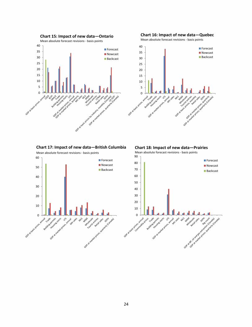
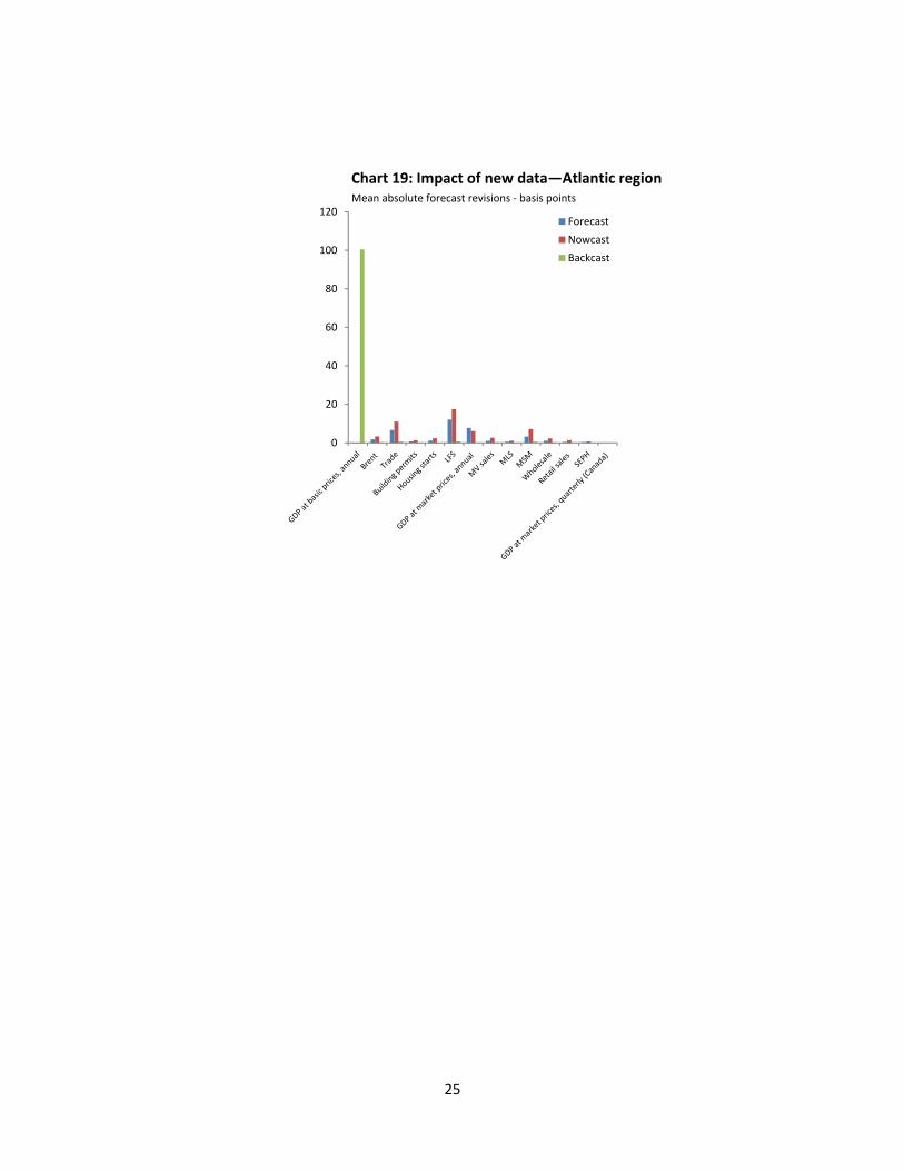
As previously discussed, the DFM can be used to decompose the news component of each

economic data release. Looking at the news provides a better understanding of the importance of

individual predictors for nowcasting GDP. Charts 15 to 19 show the mean absolute revision to the

model’s forecast for each data release by forecast period. For example, in Ontario the red line shows

0

0.5

1

1.5

2

2.5

3

Nov

Jan

Feb

Apr

May Jul

Sep

Oct

Dec

Feb

Mar

May Jul

Aug

Oct

Nov

Jan

Mar

Apr

Jun

Aug

Sep


Chart 10: RMSFE—Ontario

DFMMIDASAR

0

0.2

0.4

0.6

0.8

1

1.2

1.4

1.6

1.8

2

Nov

Jan

Feb

Apr

May Jul

Sep

Oct

Dec

Feb

Mar

May Jul

Aug

Oct

Dec Jan

Mar

May Jun

Aug

Sep


Chart 11: RMSFE—Quebec

DFMMIDASAR

0

0.5

1

1.5

2

2.5

Nov

Jan

Feb

Apr

Jun

Jul

Sep

Nov

Dec

Feb

Apr

May Jul

Aug

Oct

Dec Jan

Mar

May Jun

Aug

Oct


Chart 12: RMSFE—British Columbia

DFM

MIDASAR

0

0.5

1

1.5

2

2.5

3

3.5

Nov

Jan

Feb

Apr

Jun

Jul

Sep

Nov

Dec

Feb

Apr

May Jul

Sep

Oct

Dec Jan

Mar

May Jun

Aug

Oct


Chart 14: RMSFE—Atlantic region

DFM

MIDAS

AR

0

0.5

1

1.5

2

2.5

3

3.5

Nov

Jan

Feb

Apr

Jun

Jul

Sep

Nov

Dec

Feb

Apr

May Jul

Sep

Oct

Dec Jan

Mar

May Jun

Aug

Oct


Chart 13: RMSFE—Prairies

DFM

MIDAS

AR

23

that on average during the nowcast period, a release of Labour Force Survey data would change the

forecast for Ontario GDP growth by around 35 basis points.

The impact of individual data releases can vary across provinces and forecast periods. However,

the general trend is that the release of provincial GDP at basic prices has the single largest impact and

data releases during the nowcast periods have the next‐largest impact, followed by the forecast periods.

During the backcast period, most of the data releases do not include any news except for provincial GDP

at basic prices. This is because GDP at basic prices is very relevant for predicting provincial GDP at

market prices and is the only series released for the reference year, whereas all other data released

during the backcast period are for a future reference period and thus have no relevance. In terms of

specific data releases, the LFS contains the largest amount of news (apart from GDP at basic prices).

Other important predictors are the monthly survey of manufacturing as well as merchandise trade

releases. In the case of Ontario, where international predictors are included, the exchange rate (CEER),

commodity prices, CFNAI and GRACE all have large impacts on the predictions. This is intuitive,

considering the importance of international trade in Ontario and Canada’s close ties to the United

States.

Finally, the quarterly and monthly GDP measures produced by Ontario and Quebec do not

produce large forecast revisions. There are two potential explanations for this. First, the provincial GDP

data are released with a slightly longer lag than other data, such as the Labour Force Survey. Because

these measures are constructed using much of the same publicly available information already

incorporated into the model, they do not contain much additional news. Second, we do not impose a

direct relationship between their measures and Statistics Canada’s GDP estimates. As previously

mentioned, their series are estimates benchmarked to Statistics Canada’s annual GDP measures, and are

revised historically to be consistent with annual GDP after its release. We nevertheless include the series

because it is possible that they may provide valuable information for the forecasts in real time, although

we do not have the data vintages to quantify their impact.

24

0

5

10

15

20

25

30

35

40

Chart 15: Impact of new data—OntarioMean absolute forecast revisions ‐ basis points

Forecast

Nowcast

Backcast

0

5

10

15

20

25

30

35

40

Chart 16: Impact of new data—QuebecMean absolute forecast revisions ‐ basis points

Forecast

Nowcast

Backcast

0

10

20

30

40

50

60Forecast

Nowcast

Backcast

0

10

20

30

40

50

60

70

80

90

Chart 18: Impact of new data—PrairiesMean absolute forecast revisions ‐ basis points

Forecast

Nowcast

Backcast

Chart 17: Impact of new data—British Columbia Mean absolute forecast revisions ‐ basis points

25

0

20

40

60

80

100

120Forecast

Nowcast

Backcast

Chart 19: Impact of new data—Atlantic region Mean absolute forecast revisions ‐ basis points

26

5. ConclusionThis paper proposes a medium‐sized DFM to nowcast annual provincial GDP growth, and as a

by‐product we construct a monthly indicator of provincial economic activity. The provincial GDP data

pose several challenges: they are released only at annual frequency with a significant lag, and there is a

noisy advance release in the form of GDP at basic prices. We design our model to explicitly address all

these issues. We also investigate the use of provincial, national and international data in our nowcasting

exercise. We find that in most cases, using only provincial data to estimate the factors improves the

results, as does targeting larger regional aggregates. We show that the model performs well both in‐

sample and out‐of‐sample. The measures of economic activity fit the data well on an annual basis and

capture the dynamics of important economic events over history, while conveying the heterogeneous

regional responses to these events. They also provide more timely indications of business‐cycle turning

points and are able pick up shorter periods of economic contraction that would not be observed in the

annual average. In a pseudo real‐time exercise, we show the model produces more accurate nowcasts

than traditional simple benchmarks, such as univariate AR models. It also performs well against more

sophisticated benchmarks such as MIDAS models.

27

Appendix

Table 1: Variable list

Variable Timing Region Pub. lag (months)

Freq. Avail. from

Transf. Source

GDP at basic prices Week 1 Provincial 5 A 1984 4 Statistics Canada

CEER Week 1 National 1 M Jan‐92 2 Bank of Canada

BCPI Week 1 National 1 M Jan‐72 2 Bank of Canada

GRACE Week 1 International 2 M Mar‐92 0 Bank of Canada

WCS pricea Week 1 National 1 M Jan‐72 2 F.O.B. Hardisty, Alberta

Brent priceb Week 1 National 1 M Jan‐72 2 Intercontinental Exchange

Merchandise exports

Week 1 National 2 M Jan‐88 2 Statistics Canada

Merchandise imports


Merchandise exports

Week 1 Provincial 2 M Jan‐88 2 Statistics Canada

Merchandise imports


Building permits Week 2 National 2 M Jan‐77 2 CMHC

Building permits Week 2 Provincial 2 M Jan‐77 2 CMHC

Housing starts Week 2 National 1 M Jan‐90 2 CMHC

Housing starts Week 2 Provincial 1 M Jan‐90 2 CMHC

Real GDP at market price

Week 2 Provincial 11 A Jun‐05 4 Statistics Canada

Employment—LFS Week 2 Provincial 1 M Jan‐76 3 Statistics Canada

Unemployment—LFS


Working age population—LFS


Real GDP at market price—Ontario Financed

Week 2 Provincial 4 Q Q1‐81 5 Ontario Ministry of Finance

New MV sales, units


New MV sales, dollars


MLS resales Week 3 National 1 M Jan‐88 2 CREA

Average home price

Week 3 Provincial 1 M Jan‐88 2 CREA

MLS resales Week 3 Provincial 1 M Jan‐88 2 CREA

Manufacturing shipments


Wholesale trade Week 3 Provincial 2 M Jan‐93 2 Statistics Canada

Tourist entriese Week 3 Provincial 2 M Jan‐92 2 Statistics Canada

Retail sales Week 3 Provincial 2 M Jan‐91 2 Statistics Canada

28

Chicago Fed National Activity Index

Week 4 International 1 M Mar‐67 0 Federal Reserve Bank of Chicago

Average hourly earnings


Average weekly hours worked


Drilling rig counta Week 4 National 0 M Jan‐68 2 Baker‐Hughes

GDP at basic pricesc—ISQ

Week 4 Provincial 3 M Jan‐97 2 Institut de la Statistique du Québec

Real GDP at market price—ISQc

Week 4 Provincial 3 Q Q1‐81 5 Institut de la Statistique du Québec

GDP at basic prices Week 4 National 2 M Jan‐81 2 Statistics Canada

GDP at basic prices, manufacturing


GDP at basic prices, wholesale


GDP at basic prices, retail


GDP at basic prices, oil and gas extractiona


US GDP Week 4 International 1 Q Q1‐47 5 Bureau of Economic Analysis

GDP at market prices

Week 4 National 2 Q Q1‐81 5 Statistics Canada

Note: The transformation applied to each of the series: 0 = No change, 2 = 12‐month log difference, 3 = 12‐month difference, 4 = log difference, and 5 = 4‐quarter log difference. Variables with a superscript are only included for the following provinces or regions: a) Alberta and Prairies only b) Newfoundland and Atlantic region only c) Quebec only d) Ontario only e) Ontario, Quebec, Alberta and British Columbia.

29

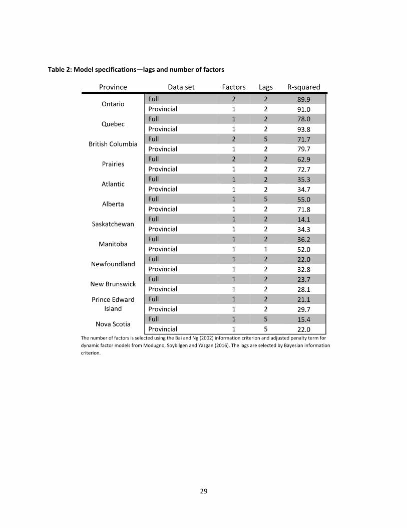
Table 2: Model specifications—lags and number of factors

Province Data set Factors Lags R‐squared

Ontario Full 2 2 89.9

Provincial 1 2 91.0

Quebec Full 1 2 78.0

Provincial 1 2 93.8

British Columbia Full 2 5 71.7

Provincial 1 2 79.7

Prairies Full 2 2 62.9

Provincial 1 2 72.7

Atlantic Full 1 2 35.3

Provincial 1 2 34.7

Alberta Full 1 5 55.0

Provincial 1 2 71.8

Saskatchewan Full 1 2 14.1

Provincial 1 2 34.3

Manitoba Full 1 2 36.2

Provincial 1 1 52.0

Newfoundland Full 1 2 22.0

Provincial 1 2 32.8

New Brunswick Full 1 2 23.7

Provincial 1 2 28.1

Prince Edward Island

Full 1 2 21.1

Provincial 1 2 29.7

Nova Scotia Full 1 5 15.4

Provincial 1 5 22.0 The number of factors is selected using the Bai and Ng (2002) information criterion and adjusted penalty term for

dynamic factor models from Modugno, Soybilgen and Yazgan (2016). The lags are selected by Bayesian information

criterion.

30

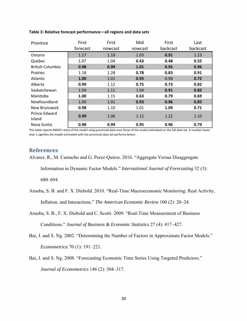
Table 3: Relative forecast performance—all regions and data sets

Province First forecast

First nowcast

Mid nowcast

First backcast

Last backcast

Ontario 1.17 1.18 1.03 0.91 1.23

Quebec 1.07 1.04 0.43 0.48 0.55

British Columbia 0.98 0.99 1.01 0.95 0.96

Prairies 1.18 1.28 0.78 0.83 0.91

Atlantic 1.00 1.01 0.95 0.98 0.72

Alberta 0.99 1.12 0.75 0.73 0.82

Saskatchewan 1.04 1.11 1.04 0.91 0.82

Manitoba 1.00 1.15 0.63 0.79 0.69

Newfoundland 1.00 1.01 0.93 0.96 0.85

New Brunswick 0.98 1.10 1.01 1.09 0.71

Prince Edward Island

0.99 1.06 1.12 1.22 1.10

Nova Scotia 0.98 0.99 0.95 0.96 0.79 This table reports RMSFE ratios of the model using provincial data over those of the model estimated on the full data set. A number lower

than 1 signifies the model estimated with the provincial data set performs better.

ReferencesAlvarez, R., M. Camacho and G. Perez-Quiros. 2016. “Aggregate Versus Disaggregate

Information in Dynamic Factor Models.” International Journal of Forecasting 32 (3):

680–694.

Aruoba, S. B. and F. X. Diebold. 2010. “Real-Time Macroeconomic Monitoring: Real Activity,

Inflation, and Interactions.” The American Economic Review 100 (2): 20–24.

Aruoba, S. B., F. X. Diebold and C. Scotti. 2009. “Real-Time Measurement of Business

Conditions.” Journal of Business & Economic Statistics 27 (4): 417–427.

Bai, J. and S. Ng. 2002. “Determining the Number of Factors in Approximate Factor Models.”

Econometrica 70 (1): 191–221.

Bai, J. and S. Ng. 2008. “Forecasting Economic Time Series Using Targeted Predictors.”

Journal of Econometrics 146 (2): 304–317.

31

Bańbura, M., D. Giannone, M. Modugno and L. Reichlin. 2012. “Now-Casting and the Real-

Time Data Flow.” Working Paper ECARES No. ECARES 2012-026. Université Libre de

Bruxelles.

Bańbura, M. and M. Modugno. 2014. “Maximum Likelihood Estimation of Factor Models on

Datasets with Arbitrary Pattern of Missing Data.” Journal of Applied Econometrics 29 (1):

133–160.

Barnett, R., K. Charbonneau and G. Poulin-Bellisle. 2016. “A New Measure of the Canadian

Effective Exchange Rate.” Bank of Canada Staff Discussion Paper No. 2016–1.

Barnett, R. and P. Guérin. 2013. “Monitoring Short-Term Economic Developments in Foreign

Economies.” Bank of Canada Review (Summer): 22–31.

Beaulieu, E. 2000. “The Canada-U.S. Free Trade Agreement and Labour Market Adjustment in

Canada.” Canadian Journal of Economics/Revue Canadienne d’économique 33 (2): 540–

563.

Beine, M. and S. Coulombe. 2003. “Regional Perspectives on Dollarization in Canada.” Journal

of Regional Science 43 (3): 541–570.

Binette, A. and J. Chang. 2013. “CSI: A Model for Tracking Short-Term Growth in Canadian

Real GDP.” Bank of Canada Review (Summer): 3–12.

Binette, A., T. Chernis and D. de Munnik. 2017. “Global Real Activity for Canadian Exports:

GRACE.” Bank of Canada Staff Discussion Paper No. 2017–2.

Boivin, J. and S. Ng. 2006. “Are More Data Always Better for Factor Analysis?” Journal of

Econometrics 132 (1): 169–194.

Bragoli, D. and M. Modugno. 2016. “A Nowcasting Model for Canada: Do U.S. Variables

Matter?” SSRN Scholarly Paper No. ID 2772899.

32

Burns, A. F. and W. C. Mitchell. 1946. Measuring Business Cycles. National Bureau of

Economic Research.

Camacho, M. and G. Perez-Quiros. 2010. “Introducing the Euro-STING: Short-Term Indicator

of Euro Area Growth.” Journal of Applied Econometrics 25 (4): 663–694.

Carlino, G. and R. DeFina. 1998. “The Differential Regional Effects of Monetary Policy.” The

Review of Economics and Statistics 80 (4): 572–587.

Cawthray, J., C. Gaudreault and R. Lamy. 2002. “Monitoring Future Economic Growth in

Canadian Provinces with New Leading Economic Indexes.” Department of Finance

Canada Working Paper No. 2002–02.

Chernis, T. and R. Sekkel. 2017. “A Dynamic Factor Model for Nowcasting Canadian GDP

Growth.” Bank of Canada Staff Working Paper No. 2017–2.

Clements, M. P. and A. B. Galvão. 2008. “Macroeconomic Forecasting with Mixed-Frequency

Data.” Journal of Business & Economic Statistics 26 (4): 546–554.

Crone, T. M. and A. Clayton-Matthews. 2005. “Consistent Economic Indexes for the 50 States.”

The Review of Economics and Statistics 87 (4): 593–603.

Croushore, D. and T. Stark. 2002. “Forecasting with a Real-Time Data Set for

Macroeconomists.” Journal of Macroeconomics 24 (4): 507–531.

Croushore, D. and T. Stark. 2003. “A Real-Time Data Set for Macroeconomists: Does the Data

Vintage Matter?” The Review of Economics and Statistics 85 (3): 605–617.

Dahlhaus, T., J.-D. Guénette and G. Vasishtha. 2015. “Nowcasting BRIC+M in Real Time.”

Bank of Canada Staff Working Paper No. 2015–38.

Demers, F. and D. Dupuis. 2005. “Forecasting Canadian GDP: Region-Specific versus

Countrywide Information.” Bank of Canada Staff Working Paper No. 2005-31.

33

DeSerres, A. and R. Lalonde. 1994. “Symétrie des chocs touchant les régions canadiennes et

choix d’un régime de change.” Bank of Canada Staff Working Paper No. 1994-9.

Doz, C., D. Giannone and L. Reichlin. 2012. “A Quasi–Maximum Likelihood Approach for

Large, Approximate Dynamic Factor Models.” The Review of Economics and Statistics 94

(4): 1014–1024.

Evans, M. D. D. 2005. “Where Are We Now? Real-Time Estimates of the Macroeconomy.”

International Journal of Central Banking 1 (2): 127–175.

Forni, M., M. Hallin, M. Lippi and L. Reichlin. 2000. “The Generalized Dynamic-Factor Model:

Identification and Estimation.” The Review of Economics and Statistics 82 (4): 540–554.

Fratantoni, M. and S. Schuh. 2003. “Monetary Policy, Housing, and Heterogeneous Regional

Markets.” Journal of Money, Credit, and Banking 35 (4): 557–589.

Galbraith, J. W. and G. Tkacz. 2017. “Nowcasting with Payment Systems Data.” International

Journal of Forecasting. Forthcoming.

Georgopoulos, G. 2009. “Measuring Regional Effects of Monetary Policy in Canada.” Applied

Economics 41 (16): 2093–2113.

Ghysels, E., P. Santa-Clara and R. Valkanov. 2004. “The MIDAS Touch: Mixed Data Sampling

Regression Models.” CIRANO Working Paper No. 2004s–20.

Ghysels, E., A. Sinko and R. Valkanov. 2007. “MIDAS Regressions: Further Results and New

Directions.” Econometric Reviews 26 (1): 53–90.

Giannone, D., S. Agrippino and M. Modugno. 2013. “Nowcasting China Real GDP.” Working

Paper.

34

Giannone, D., L. Reichlin and D. Small. 2008. “Nowcasting: The Real-Time Informational

Content of Macroeconomic Data.” Journal of Monetary Economics 55 (4): 665–676.

Kopoin, A., K. Moran and J.-P. Paré. 2013. “Forecasting Regional GDP with Factor Models:

How Useful Are National and International Data?” Economics Letters 121 (2): 267–270.

Lamy, R. and P. Sabourin. 2001. “Monitoring Regional Economies in Canada with New High-

Frequency Coincident Indexes.” Department of Finance Canada Working Paper No. 2001-

05.

Luciani, M. (2014). “Large-Dimensional Dynamic Factor Models in Real-Time: A Survey.”

SSRN Scholarly Paper No. ID 2511872.

Mariano, R. S. and Y. Murasawa. 2003. “A New Coincident Index of Business Cycles Based on

Monthly and Quarterly Series.” Journal of Applied Econometrics 18 (4): 427–443.

Matheson, T. 2011. “New Indicators for Tracking Growth in Real Time.” SSRN Scholarly Paper

No. ID 1770369.

Modugno, M., B. Soybilgen and M. E. Yazgan. 2016. “Nowcasting Turkish GDP and News

Decomposition.” Board of Governors of the Federal Reserve System (U.S.), Finance and

Economics Discussion Series No. 2016-044.

Orphanides, A. 2001. “Monetary Policy Rules Based on Real-Time Data.” American Economic

Review 91 (4): 964–985.

Owyang, M. T., J. Piger and H. J. Wall. 2005. “Business Cycle Phases in U.S. States.” The

Review of Economics and Statistics 87 (4): 604–616.

Paredes, J., J. J. Pérez and G. Perez-Quiros. 2015. “Fiscal Targets. A Guide to Forecasters?”

SSRN Scholarly Paper No. ID 2584877.

35

Salem, M. 2003. “Are Some Regions More Sensitive to Business Cycles?” Latest Developments

in the Canadian Economic Accounts, Statistics Canada 13-605-X.

Stock, J. H. and M. W. Watson. 1989. “New Indexes of Coincident and Leading Economic

Indicators.” NBER Macroeconomics Annual 4: 351–394.

Stock, J. H. and M. W. Watson. 1999. “Forecasting inflation.” Journal of Monetary Economics

44 (2): 293–335.

Stock, J. H. and M. W. Watson. 2002. “Macroeconomic Forecasting Using Diffusion Indexes.”

Journal of Business & Economic Statistics 20 (2): 147–162.

Trefler, D. 2004. “The Long and Short of the Canada-U. S. Free Trade Agreement.” American

Economic Review 94 (4): 870–895.

Wilson, T.A. 1985. “Lessons of the Recession.” The Canadian Journal of Economics 18 (4):

693–722.

a three‐frequency dynamic factor model for nowcasting ... · we are extremely thankful to kevin...

Documents