A Theory of Individualism, Collectivism and

Economic Outcomes

Kartik Ahuja, Mihaela van der Schaar and William R. Zame∗

July 4, 2016

∗Ahuja: Department of Electrical Engineering, UCLA, Los Angeles, CA 90095; ahu-

jak@ucla.edu. van der Schaar: Department of Electrical Engineering, UCLA, Los Angeles,

CA 90095; mihaela@ee.ucla.edu. Zame: Department of Economics, UCLA, Los Angeles,

CA 90095; zame@econ.ucla.edu. We are grateful to John Asker, Moshe Buchinsky, Dora

Costa and a seminar audience at UCLA for helpful comments. Research support to Ahuja

and van der Schaar was provided by the U.S. Office of Naval Research Mathematical Data

Science Program; additional support to Ahuja was provided by the Guru Krupa Foun-

dation. Any opinions, findings, and conclusions or recommendations expressed in this

material are those of the authors and do not necessarily reflect the views of any funding

agency.

arX

iv:1

512.

0123

0v2

[ph

ysic

s.so

c-ph

] 1

Jul

201

6

Abstract

This paper presents a dynamic model to study the impact on the

economic outcomes in different societies during the Malthusian Era

of individualism (time spent working alone) and collectivism (com-

plementary time spent working with others). The model is driven

by opposing forces: a greater degree of collectivism provides a higher

safety net for low quality workers but a greater degree of individualism

allows high quality workers to leave larger bequests. The model sug-

gests that more individualistic societies display smaller populations,

greater per capita income and greater income inequality. Some (lim-

ited) historical evidence is consistent with these predictions.

It is widely agreed (see Landes (1998) for instance) that culture has an

important influence on social outcomes and economic outcomes but there is

little agreement on which aspects of culture are important for which eco-

nomic outcomes, whether these aspects are different in different eras, and

through what mechanisms culture operates. This paper focuses on the im-

pact of one aspect of culture – the degree of individualism vs. collectivism –

on the population, income and income distribution of societies in the period

between the Neolithic Revolution and the Industrial Revolution – a period in

which life was (in the words of Thomas Hobbes) “nasty, brutish and short,”

in which agriculture was the mainstay of economic activity and societies were

stuck in the Malthusian trap, which Clark (2008), Clark (2007), Ashraf and

Galor (2011) and Galor (2005) (and others) characterize by subsistence with

no technological progress and little or no growth in either population or in-

come. We provide and analyze a model of the mechanism through which

2

individualism and collectivism act. Our model predicts that societies that

are more individualistic (less collectivistic) tend to have smaller populations,

higher mean incomes, and greater income inequality. Perhaps surprisingly,

our model predicts that technological differences may matter a great deal

for the size of the population but not for income or income inequality. We

offer some historical evidence that is consistent with the predictions of the

model.(Clark (2008), Clark (2007), Ashraf and Galor (2011) and Galor (2005)

have offered mathematical models of the Malthusian trap, but these models

do not offer an explanation of how or why cross-cultural differences – in par-

ticular, differences in the degree of individualism and collectivism – might

have influenced outcomes in this period. This is precisely the explanation

our mathematical model is designed to provide. Gorodnichenko and Roland

(2011b), Gorodnichenko and Roland (2011a), Roland and Gorodnichenko

(2010) offer an analysis of the impact of indivualism vs. collectivism in

the era after the Industrial Revolution. They argue that individualism re-

wards status and hence promotes innovation which in turn promotes growth.

However it does not seem that this explanation can explain the impact of

individualism vs. collectivism in the Malthusian Era – in which there was no

growth.)

We follow Hofstede (1984) in viewing individualism as an aspect of cul-

ture that is associated with traits like acting independently and taking care

of oneself and collectivism as an aspect that is associated with mutual depen-

dence amongst the members of the group. As in Hofstede (1984), we view

individualism and collectivism as aspects of the culture of a society, which

might or might not arise as aspects of the political structure. We formalize

3

the degree of individualism as the fraction of time that members of society

work by themselves and enjoy only the output of their own activity and the

degree of collectivism as the complementary fraction of time that members

of society work together and enjoy the output of the group activity. We

take these fractions as a universal social norm that is observed by all the

members of society and not as choices of different members of society (but

these fractions differ across societies). The societal division of time/labor

matters because individuals differ in ability (physical strength, skill, etc.).

When working individually, output per unit time depends on the individ-

ual’s ability; when working collectively, output per unit time depends on the

average ability of society. When working collectively the less able members

of society produce more per unit time than when working alone – so a greater

degree of collectivism provides a social “safety net” for the low ability mem-

bers of society. On the other hand, when working collectively the more able

members of society produce less per unit time than when working alone –

so a greater degree of collectivism decreases the wealth of the high ability

members of society and hence the bequests they leave (to new-borns) when

they die. Because income from production and inheritance from bequests

both affect the path of individual wealth and hence lifespan, the degree of

collectivism and the complementary degree of individualism create opposing

forces ; the balance of these forces (and others) plays out in a complicated

and subtle way.

4

1 Model

The features of the model that we develop here are intended to represent

(some aspects of) steady-state outcomes of societies in the Malthusian Era,

in which (changing) technology does not play an important role.

Before giving a formal mathematical description of the model, we begin

with an informal verbal description that expands on what we have already

said in the Introduction. We consider a world populated by a continuum

of individuals of two types either Low quality or High quality.1 Time is

continuous and the horizon is infinite. The lifecycle of an individual is:

• individuals are born and come into an inheritance;

• during their lifetimes, individuals consume and produce;

• individuals die and leave a bequest for succeeding individuals.

While they are alive and producing, each individual spends a fraction of its

time working alone and consuming the output of its individual production,

and the complementary fraction of its time working with others and sharing

(equally) in the joint production. We interpret these fractions as (proxies for)

the degree of individualism and the degree of collectivism of the society.2 We

1Allowing for more quality levels would complicate the analysis without altering the

qualitative conclusions.2For example, Leibbrandt, Gneezy and List (2013) show that lake based fishing areas

are more individualistic and involve more isolated work by the individuals, while sea based

fishing areas are more collectivistic and involve more collective work by the individuals.

5

view these fractions as social norms which are the same across all individuals

in the society, rather than as individual choices. (We are agnostic about

the origins of these social norms; one possibility is that they are imposed

by a governmental structure but there are many other possibilities.) When

individuals work alone, their output depends on their own quality; when

individuals work with others, their output depends on the average quality of

society. In both modes, output is subject to congestion: productivity is less

when the total population is greater. (This congestion is an essential part of

Clark’s argument for why societies remain in the Malthusian trap and plays

an important role in our model as well.) During their lifetimes, individuals

consume at a constant rate. (We discuss alternative assumptions below)

Some individuals produce less than they consume and eventually consume

their entire inheritance; at that point their wealth is zero and they die in

poverty. Individuals who do not die in poverty eventually die of natural

causes. Individuals who die with positive wealth leave that wealth as a

bequest to the new-born.

We now turn to the formal mathematical description. We consider a

continuous-time model with a continuum of individuals. Some individuals

are of High quality and some are of Low quality; it is convenient to index

quality by Q = 0, 1 (Low, High).3 The state of society at each moment

of time is described by the population distributions P0,P1; PQ(x, t) is the

population of individuals of quality Q who have wealth less than or equal to

3The individuals in our model are productive adults, so we view their quality as fixed

and not changing over their lifetimes.

6

x at time t. The population of individuals of quality Q at time t is

PQ(t) = limx→∞PQ(x, t)

Thus the total population at time t is

P (t) = P0(t) + P1(t)

and the average quality at time t is

Q̄(t) = [0 · P0(t) + 1 · P1(t)]/P (t) = P1(t)/P (t)

Individuals are born at the constant rate λf and die natural deaths at the

constant rate λd.4 Half of all newborns are of High quality and half are of

Low quality. (The assumption that the proportions of new-borns of High and

Low quality are constant is made only for simplicity: none of the qualitative

results would change if we assumed that quality is partly inheritable, so that

the proportions of High and Low quality newborns depend on the current

population. The assumption of equal proportions is made only to simplify

the algebra.) As we discuss below, some individuals also die in poverty.

While they are alive, individuals produce and consume. We assume that

each individual spends a fraction z of its time working alone and the remain-

ing fraction 1 − z working with others. As noted, we identify z with the

degree of individualism of the society and 1− z as the degree of collectivism.

4 Clark (2008) argues that the fertility rate is an increasing function of the wealth of

society and that the death rate is a decreasing function of the wealth of society. Those fea-

tures could be incorporated into our model without changing the qualitative conclusions,

although at the expense of substantial mathematical complication.

7

When an individual works alone its production depends on its own quality

and is consumed entirely by the individual; when it works with others its

production depends on the average quality of society (at the given moment

of time) and is shared; in both modes, productivity is subject to conges-

tion and so diminishes with increasing population. For simplicity, we assume

productivity is linear in quality so productivity of an individual of quality

Q = 0, 1 at a given time t when population is P (t) and average quality is Q̄(t)

is [Q − cP (t)] when working alone and [γQ̄(t) − cP (t)] when working with

others, where γ is a parameter that represents the efficiency of group pro-

duction. (Our assumptions about functional forms are made for tractability;

our assumption that low quality individuals working alone produce nothing

is simply a normalization. As we will see below, the essential point is that,

when working alone, low quality individuals produce less than they consume

so that their wealth decreases. (The role of the parameter γ will be discussed

in greater detail below.) Hence the overall productivity of an individual of

quality Q = 0, 1 is

FQ(t) = z[Q− cP (t)] + (1− z)[γQ̄(t)− cP (t)]

= zQ+ (1− z)γQ̄(t)− cP (t)(1)

We emphasize that Q is the innate and fixed quality of the (adult) individual

and that z, 1−z are characteristics of the society, and not individual choices.

We assume each individual consumes at the constant (subsistence) rate

k; for algebraic simplicity (only) we take k = 1/2. Hence the rate of pro-

duction net of consumption for an individual with quality Q is FQ(t)− 1/2.

Individuals who die at time t leave a fraction η < 1 of their wealth as an

8

inheritance for individuals born at the same time t; the remaining fraction

1− η of this wealth is lost in storage. We write y(t0) as the (common) inher-

itance of individuals who are born at time t0. So an individual of quality Q

born at time t0 begins life with wealth Xq(t0) = y(t0); and its wealth changes

during its lifetime at the rate:

dXQ(t)/dt = FQ(t)− 1/2 (2)

We stress that an individual’s wealth may shrink or grow; if it shrinks, it may

eventually shrink to 0 before the individual dies of natural causes in which

case the individual dies in poverty. Of course individuals who die in poverty

do not leave an inheritance. In our analysis, we show that the system has a

unique non-degenerate steady state. In this steady state, dX0(t)/dt < 0 and

dX1(t)/dt > 0 so the wealth of low quality individuals shrinks and the wealth

of high quality individuals grows; it follows that some low quality individuals

die in poverty but no high quality individuals die in poverty.

We have defined the state of society at time t in terms of the population

distributions P0,P1; however in analyzing the evolution of society it is more

convenient to work with the population densities p0, p1. By definition,

PQ(x, t) =

∫ x

0

pQ(x̂, t) dx̂

Working with densities is more convenient because their evolution is deter-

mined by the following evolution equations, which are based on the principle

of mass conservation:

∂p0(x, t)

∂t+∂p0(x, t)

∂x[F0(t)− 1/2] = −λdp0(x, t)

∂p1(x, t)

∂t+∂p1(x, t)

∂x[F1(t)− 1/2] = −λdp1(x, t) (3)

9

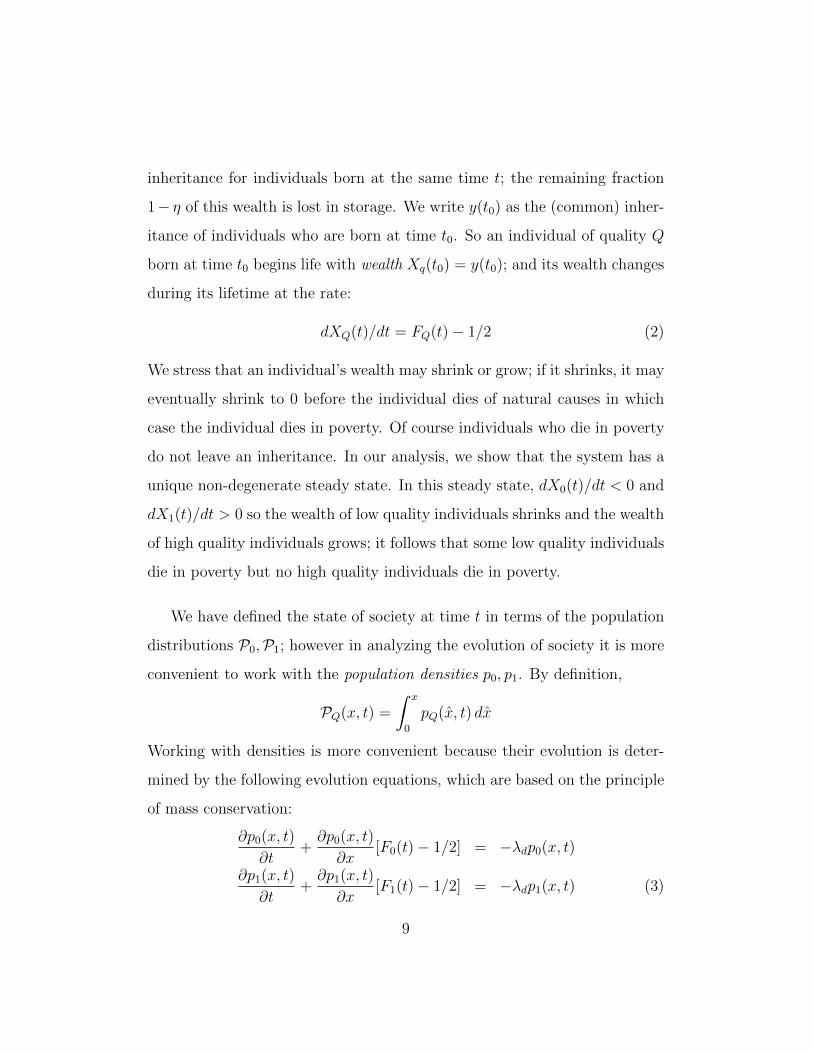
BirthLow quality

individual

High quality

individual

Society

Natural death/

Poverty death

Natural death/

Poverty death

Death Death

(1 − 𝑧)(𝛾 𝑄 𝑡 − 𝑐 𝑃 𝑡 )𝑄 = 0 𝑄 = 1

(1 − 𝑧)(𝛾 𝑄 𝑡 − 𝑐 𝑃 𝑡 ) Individual’s share of the collective output

Figure 1: Individual’s life span

The first term on the left hand sides of these PDE (3) represents the rate

of change of the population density at a given wealth level and the second

term is the divergence of the flux; the right hand sides represents the rate

at which individuals die due to natural causes. Note that neither deaths in

poverty nor births appear in the evolution equations. This is because deaths

in poverty only occur at x = 0 and births only occur at x = y(t) (inheritance

at time t); deaths in poverty and births enter into the behavior of the system

as “boundary conditions” at 0, x = y(t) (see the Appendix). Note that these

evolution equations are coupled because productivity of agents of each quality

depends on the total population rather than on the population of the given

quality. Note too that the “boundary” x = y(t) is moving because inheritance

y(t) is a function of the population distributions and hence depends on time.

We summarize the life-span of an individual in Figure 1.

10

1.1 Steady State

We are interested in societies in the steady state; because we are interested

in the (long) period after the Neolithic Revolution and before the Industrial

Revolution, during which there was little growth or change (see for instance

Clark (2008)), this seems reasonable. We define the steady state as the state

of the society in which the distribution of individuals (of each type) across

wealth levels is unchanging over time; i.e., ∂pQ(x, t)/∂t ≡ 0 for Q = 0, 1. In

the the steady state, the birth and (overall) death rate are constant and equal,

so the populations P0(t), P1(t), P (t) are constant; write P s0 , P

s1 , P

s for the

steady state values. Because the population is constant, so are the average

quality Qs = P s1 /P

s, the productivities of individuals of each quality F sQ =

zQ + (1 − z)Qs − cP s, and inherited wealth Y s. (All these values will be

determined endogenously by the parameters of the model and the condition

that the society is in steady state.)

There is always a degenerate steady state in which population is iden-

tically 0. In order to guarantee that a non-degenerate steady state exists,

we need four assumptions, which will be maintained in what follows without

further comment.

Assumptions

1. λd < λf < 2λd

2. λd/λf < γ

11

3. 0 < z < λdλf

4. 1/(1 +[1−λd/λf ]

ln( 12[1−λd/λf ]

)) < η

Some comments on these assumptions are in order. If the natural birth rate

were less then the natural death rate then the population of society would

shrink to 0 in the long run so the only steady state would be degenerate.

Similar reasoning explains the second assumption. To see why the third

assumption is needed, suppose for a moment that z = 0, so that the society

were completely collectivist. In a completely collectivist society, individual

output depends only on average quality and not on individual quality, and

hence net output in a steady state would be Q̄s−cPs−1/2. If net output were

positive, inheritance would blow up; if net output were negative, inheritance

would shrink to 0. Hence in the steady state, net output must be 0. But this

means that no individuals die in poverty; since the average quality of newly

born agents is 1/2, the steady state average quality of the population must

also be 1/2 and the steady state population must be 0. Hence a completely

collectivist society cannot persist in a non-degenerate steady state. Similar

reasoning shows that an extremely individualistic society cannot persist in a

non-degenerate steady state; the necessity of the given upper bound is derived

in the proof of Theorem 1. (Put differently: our model cannot apply to a

society that is too collectivist or too individualistic.) The last assumption

asserts that the loss of wealth in inheritance is not too great. (Recall that

we have already assumed η < 1; i.e. some wealth is lost in inheritance.) If η

were below the given bound then, as the proof of Theorem 1 demonstrates,

the population of low quality individuals would go to 0, which would once

12

0 0.05 0.1 0.15 0.2 0.252

3

4

5

6

7

8

Wealth level (x)

Popu

latio

n D

ensi

ty o

f In

divi

dual

s

High quality individualsLow quality individuals

p0s(x)

p1s(x)

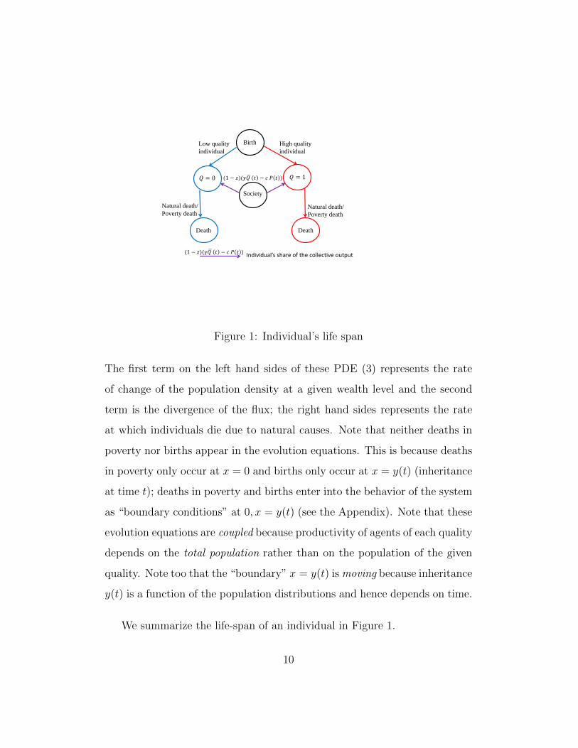
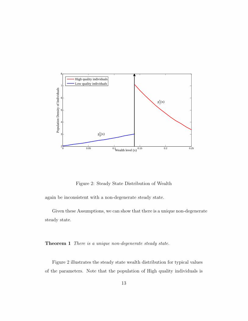
Figure 2: Steady State Distribution of Wealth

again be inconsistent with a non-degenerate steady state.

Given these Assumptions, we can show that there is a unique non-degenerate

steady state.

Theorem 1 There is a unique non-degenerate steady state.

Figure 2 illustrates the steady state wealth distribution for typical values

of the parameters. Note that the population of High quality individuals is

13

greater than that of Low quality individuals, as indeed it must be given our

assumptions.

We defer the proof of this result (and all others) to the Appendix.

2 Model Predictions

We now show that our model has strong – and perhaps surprising – implica-

tions for economic outcomes.

To understand what drives these implications, it is useful to think about

the various forces at work and how they manifest in the various aspects of the

steady state. Throughout the discussion, we take birth and death rates and

inheritability η of bequests as fixed, so that the steady state depends on the

congestion coefficient c, the group efficiency γ and the degree of individualism

z.

The forces that these parameters generate can be seen most easily by

comparing the non-degenerate steady state populations in different societies

which differ in only one of these parameters. With an obvious abuse of

language we may speak of one of these parameters being or becoming larger.

Intuitively at least we can reason as follows.

• If we hold group efficiency γ and degree of individualism z fixed then

a larger congestion parameter c generates a downward force on the

population. To see this, note that a larger c implies a more negative

14

congestion effect, so that productivity will be lower in both individ-

ual and group modes. Hence the wealth of low quality individuals

will decline more quickly and wealth of high quality individuals will

increase more slowly. From this it also follows that individuals who

die of natural causes will leave a smaller bequest, and hence that new-

born individuals will come into a smaller inheritance. In particular,

low quality individuals will begin with less wealth, spend that wealth

faster, and hence be more likely to die in poverty before they die of nat-

ural causes. So if the congestion parameter is larger then the steady

state population should be smaller.

• If we hold congestion c and degree of individualism z fixed then greater

group efficiency γ generates an upward force on the population. To

see this note that greater group efficiency means greater productivity

for both high and low quality individuals when working with others.

Hence the wealth of low quality individuals will decline more slowly and

the wealth of high quality individuals will increase more quickly. From

this, it also follows that individuals who die of natural causes will leave

a larger bequest, and hence that new-born individuals will come into

a larger inheritance. In particular, low quality individuals will begin

with greater wealth, spend that wealth more slowly, and hence be less

likely to die in poverty before they die of natural causes. So if group

efficiency is greater then the steady state population should be larger.

• However if we hold congestion c and group efficiency γ fixed then a

greater degree of individualism z generates both upward and downward

15

forces on the population. To see this note that, on the one hand,

low quality individuals produce more per unit time when working with

others than when working alone, so working with others provides low

quality workers with a “safety net.” A greater degree of individualism

lowers this “safety net”, so that the wealth of low quality workers more

quickly and they die in poverty more often. On the other hand (at least

if γ is not too large) high quality individuals produce less per until time

when working with others than when working alone. A greater degree of

individualism therefore increases the rate at which high quality workers

accumulate wealth, and hence increases the bequests they leave when

they die, which in turn implies that low quality individuals begin life

with greater wealth and tend to die in poverty less often. Evidently,

these forces work in opposite directions so the impact of the degree of

individualism on population depends on the balance between them; we

show below, the net effect depends on the relative magnitude of all the

parameters.

As Theorem 2 below demonstrates formally, these intuitions about the impact

of parameters on steady state population are indeed correct (and we can say

even more about the impact of individualism). However, we warn the reader

that, as we will see later, similar intuitions about the impact of parameters

on other economic outcomes are not correct . Although it may seem quite

surprising, neither the congestion coefficient c nor the group efficiency γ

influences mean income or income inequality.

16

Theorem 2 In the non-degenerate steady state, population depends on c, γ, z

in the following way:

(a) P s is decreasing as a function of the congestion parameter c;

(b) P s is increasing as a function of group efficiency γ

(c) for each c > 0 there is a threshold γ∗ such that

(i) if γ < γ∗ then P s is linearly increasing in z;

(ii) if γ > γ∗ then P s is linearly decreasing in z.

Theorem 2 describes the dependence of the total population on the various

parameters but is silent about the dependence of the populations of each

quality and the ratio of these populations. Perhaps surprisingly, as Theorem

3 below asserts formally this ratio is independent of all the parameters. To

understand the intuition for this conclusion, suppose the parameters change

in such a way that the population of low quality workers grows. Because

the birth rate and the ratio of low quality births to high quality births are

constant, the population of high quality workers must also grow – and, as

we show, it must grow at precisely the same rate as the population of low

quality workers, so that the ratio of the populations remains constant.

Theorem 3 In the non-degenerate steady state, the population ratio P s0 /P

s1

is independent of c, γ, z.

17

We now turn from population to income, in particular to mean income and

to income inequality. We identify income with output so the mean income

of society in the steady state is

F s = [F s0P

s0 + F s

1Ps1 ]/P s

Theorem 4 In the non-degenerate steady state, mean income is independent

of c, γ and linearly increasing in the degree of individualism z.

At first glance, Theorem 4 might seem startling. It is natural to think

of improved technology as manifested in a smaller congestion coefficient c

and a larger group efficiency γ; in view of Theorem 2 this would lead to

an increase in the size of the population. However as population increases,

so does congestion which reduces the (per capita) gains to the improved

technology; in the steady state, these forces exactly balance out. It seems

important to point out that this is not simply an artifact of our model; Ashraf

and Galor [3] argue that this is precisely what is observed in the data.

We measure income inequality in the familiar way as the Gini coefficient

of the income distribution. Because there are only two types of individuals,

the Gini coefficient takes the particularly simple form

F s1P

s1 /F

sP s − P s1 /P

s =

[P s1

P s

] [F s1

F s− 1

]

Theorem 5 In the non-degenerate steady state the Gini coefficient is inde-

pendent of c, γ and increasing in the level of individualism z.

18

3 Some Historical Evidence

As we have said before, we intend our model to be descriptive of societies in

the period between the Neolithic Revolution and the Industrial Revolution.

Although only a limited amount of data is available for this period and there

is some disagreement about its quality, it nevertheless seems appropriate to

compare the predictions of our model with the data that is available.

Our model makes use of a number of parameters: the birth and death

rates λf , λd, the fraction η of wealth that is inheritable, the coefficient c of

congestion, the group efficiency γ, and the degree z of individualism. Unfor-

tunately, none of these parameters can be observed directly. (At least, none

of these parameters were observed directly in the data that is available to

us.) What is available is an index of individualism calculated by Hofstede

(1984), which we use as a proxy for z (rescaled to lie in [0, 1]).5 In comparing

the predictions of our model with historical data we make the simple (but

perhaps heroic) assumption that birth and death rates and the fraction of

wealth that is inheritable are the same across societies. It seems completely

implausible to assume that technologies are the same across societies – and

hence that the technological parameters c, γ are the same across societies –

5A natural alternative would be to assume that z is a (monotone) Box-Cox transfor-

mation (Box and Cox, 1964) of Hofstede’s index. We have in fact computed the optimal

Box-Cox transformation and carried through the regressions after performing the optimal

Box-Cox transformation; however, there is almost no change in either the regression lines

or the fit to the data. The results of these regressions are available from the authors on

request.

19

so we focus on the predictions for mean income and Gini coefficient, which

are independent of these parameters.

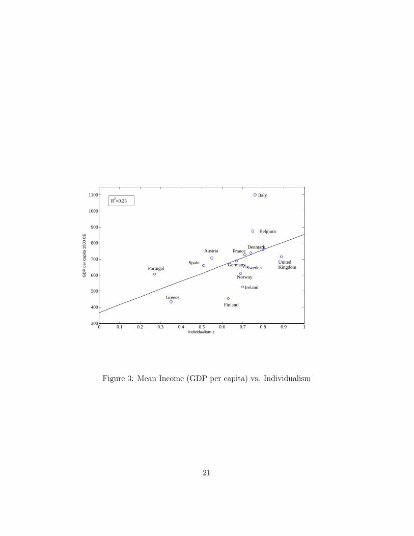
To examine the implications of Theorem 4 with historical data, we use

estimates of GDP in 1500 CE provided in Maddison (2008) for Western

Europe. We identify mean income with GDP per capita We use linear least-

squares regression to compute the best-fitting straight line; the data and

regression results can be seen in Figure 3. (Note that some of the “countries”

that appear in Figure 3 – e.g. Italy – did not exist in 1500. Maddison uses

the names to refer to the geographic areas occupied by the current countries.)

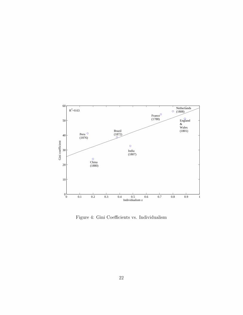
Unfortunately, we do not find any data for Gini coefficients from 1500

CE (the period of the data used above). We therefore use the estimates of

Gini coefficients given by Milanovic, Lindert and Williamson (2007). This

data from the (roughly) 100 year period 1788-1886 C.E. which might be

thought to be after the Industrial Revolution and hence not appropriate for

our model. However, for those countries in which the Industrial Revolution

arrived early (especially England, France and The Netherlands), the data

and the calculations/estimations are from the beginning of this period, which

would seem to be predominantly before the Industrial Revolution, while for

those countries (especially Brazil, China and Peru) for which the data and

the calculations/estimations are from the end of this period, the Industrial

Revolution did not in fact arrive until much later. The data and regression

results can be seen in Figure 4.

20

0 0.1 0.2 0.3 0.4 0.5 0.6 0.7 0.8 0.9 1300

400

500

600

700

800

900

1000

1100

Individualism z

GD

P p

er c

apita

150

0 C

E

SwedenPortugal

Greece

Spain

Austria

Finland

FranceDenmark

Ireland

Germany

Norway

Italy

Belgium

UnitedKingdom

R2=0.25

Figure 3: Mean Income (GDP per capita) vs. Individualism

21

0 0.1 0.2 0.3 0.4 0.5 0.6 0.7 0.8 0.9 10

10

20

30

40

50

60

Individualism z

Gin

i coe

ffic

ient

China(1880)

India(1807)

France(1788)

Netherlands(1808)

Brazil(1872)Peru

(1876)

R2=0.63

England&Wales(1801)

Figure 4: Gini Coefficients vs. Individualism

22

4 Discussion and Conclusions

This paper proposes and analyzes a model that provides a mechanism by

which the tension between individualism and collectivism can lead to different

economic outcomes in different societies. The model captures important

features of the period between the Neolithic Revolution and the Industrial

Revolution era as discussed in the work of Clark (2008) and others. The

model makes predictions about the impact of individualism and collectivism

on different societies, and these predictions seem consistent with (limited)

historical data.

We reach no conclusion as to whether individualism or collectivism is

“better” – indeed, the predictions of the model show that such a conclusion

would depend entirely on the criteria used. In particular, our prediction is

that a greater degree of individualism leads to higher mean income (GDP per

capita) but also to greater inequality; the first seems desirable, the second

does not.

The model presented above makes many simplifying assumptions – but

the model could be generalized in many dimensions (allowing for non-linear

congestion and non-constant fertility and death rates, for instance) without

qualitative changes in the conclusions. Other generalizations might allow for

the possibility that individual output and deaths due to poverty are stochas-

tic (rather than deterministic) – but such generalizations would seem to lead

to enormous complications.

23

We have confined our analysis to the steady state of the society which

seems reasonable given that we are interested in the Malthusian Era in which

there was little or no change. However even in the Malthusian era there were

shocks – famines and epidemics – which perturbed the system from its steady

state, so it would certainly be of interest to know if the steady state of our

model is at least locally stable – i.e. if the system converges to the steady

state from any initial point close to the steady state. Unfortunately, this is

an extremely complicated problem and well beyond or capabilities. Out of

the steady state the dynamics of our model are governed by a coupled pair

of PDE’s with a moving boundary constraint (and so the future evolution

of the system depends on the entire wealth distribution and not just on a

few aggregates). Such dynamical systems are well-known to be extremely

difficult to analyze – or indeed, even to simulate numerically (because the

numerical simulations can be extremely sensitive to the precise small details

of the numerical approximation).

Finally, the methodology proposed here suggests ways to think about

contemporary societies as well – although the analysis of contemporary soci-

eties will surely be more complicated because of rapidly changing technology,

growing populations and trade.

References

Ashraf, Quamrul, and Oded Galor. 2011. “Dynamics and stagnation in

the Malthusian epoch.” The American Economic Review, 101(5): 2003–

24

2041.

Box, George EP, and David R Cox. 1964. “An analysis of transforma-

tions.” Journal of the Royal Statistical Society. Series B (Methodological),

211–252.

Clark, Gregory. 2007. “The long march of history: Farm wages, popula-

tion, and economic growth, England 1209–18691.” The Economic History

Review, 60(1): 97–135.

Clark, Gregory. 2008. A farewell to alms: a brief economic history of the

world. Princeton University Press.

Galor, Oded. 2005. “From stagnation to growth: unified growth theory.”

Handbook of economic growth, 1: 171–293.

Gorodnichenko, Yuriy, and Gerard Roland. 2011a. “Individualism, in-

novation, and long-run growth.” Proceedings of the National Academy of

Sciences, 108(Supplement 4): 21316–21319.

Gorodnichenko, Yuriy, and Gerard Roland. 2011b. “Which dimensions

of culture matter for long-run growth?” The American Economic Review,

101(3): 492–498.

Hofstede, Geert. 1984. Culture’s consequences: International differences

in work-related values. Vol. 5, sage.

Landes, David S. 1998. “The wealth and poverty of nations: why some

countries are so rich and some so poor.” New York, NY: WW Noton.

25

Leibbrandt, Andreas, Uri Gneezy, and John A List. 2013. “Rise and

fall of competitiveness in individualistic and collectivistic societies.” Pro-

ceedings of the National Academy of Sciences, 110(23): 9305–9308.

Maddison, Angus. 2008. “Statistics on World Population, GDP and Per

Capita GDP, 1-2008 AD.(University of Groningen).” http://www.ggdc.

net/maddison/oriindex.htm, (accessed June 27, 2016).

Milanovic, Branko, Peter H Lindert, and Jeffrey G Williamson.

2007. “Measuring ancient inequality.” National Bureau of Economic Re-

search Working paper 13550.

Roland, Gerard, and Yuriy Gorodnichenko. 2010. “Culture, institu-

tions and the wealth of nations.” National Bureau of Economic Research

Working paper 16368.

A Mathematical Appendix

Here we present the proofs for the formal results discussed in the text. Before

we being, recall that the productivity of an individual of quality Q at time t

is:

FQ(t) = z[Q− cP (t)] + (1− z)[Q̄(t)γ − cP (t)] = zQ+ (1− z)γQ̄(t)− cP (t)

Note low quality individuals are always more productive when working col-

lectively, but whether high quality individuals are more or less productive

26

when working collectively depends on whether γQ̄(t) > 1 or γQ̄(t) < 1, and

this is determined endogenously.

Proof of Theorem 1 Since the proof is a bit roundabout, it may be

useful to begin with an overview. By definition, a steady state is a pair

of density functions p0(x, t), p1(x, t) that satisfy the evolution equations and

are independent of time t. In the steady state, the populations P s0 , P

s1 and

inheritance Y s are constant, so average quality Qs and productivities F s0 , F

s1

are also constant. Hence we can identify a steady state as a pair of functions

p0(x), p1(x) that satisfy the steady state evolution equations

∂p0(x)

∂x[F s

0 − 1/2] = −λdp0(x) (SSEE0)

∂p1(x)

∂x[F s

1 − 1/2] = −λdp1(x) (SSEE1)

and also satisfy the appropriate boundary conditions. We therefore begin

with candidate steady state populations P s0 , P

s1 and inheritance Y s (satisfying

some conditions that must hold in any steady state of the system). For

any such triple, we show that the equations SSEE0, SSEE1 admit unique

solutions which yield the given steady state quantities. We then show that

the boundary conditions uniquely pin down the unique triple of steady state

quantities that correspond to an actual steady state of the society.

We begin by considering any non-degenerate solution ps0(x), ps1(x) to the

steady state evolution equations (not necessarily satisfying boundary condi-

tions). From these, we can derive the following steady state quantities:

27

• the population of individuals with quality Q

P sQ =

∫ ∞0

psQ(x)dx (4)

• the total population

P s = P s1 + P s

0 =

∫ ∞0

[ps1(x) + ps0(x)]dx (5)

• mean quality

Qs = P s1 /(P

s0 + P s

1 ) (6)

• productivity of individuals of quality Q

F sQ = zQ+ (1− z)γQs − cP s (7)

• mean wealth

Xs =

∫∞0x[ps1(x) + ps0(x)]dx∫∞

0[ps1(x) + ps0(x)]dx

(8)

• inheritance

Y s = λdPsXsη/λfP

s = (λd/λf )Xsη (9)

Because we have assumed a non-degenerate steady state we must have P s 6= 0

so P s0 6= 0 and P s

1 6= 0. Note that the three quantities P s0 , P

s1 , Y

s determine

all the others.

We assert that in a non-degenerate steady state we must have F s0 < 1/2 <

F s1 . (Low quality individuals produce less than they consume; high quality

individuals consume less than they consume.) To show this we show that

the other possibilities are incompatible with a non-degenerate steady state.

Note first of all that the definitions and the assumption that 0 < z < 1 imply

that F s0 < F s

1 so we must rule out the only two other possibilities:

28

• 1/2 ≤ F s0 < F s

1 . If this were the case then the wealth of low qual-

ity individuals would be non-decreasing during their lifetimes and the

wealth of high quality individuals would be strictly increasing during

their lifetimes, so social wealth would be strictly increasing, which is

impossible in the steady state.

• F s0 < F s

1 ≤ 1/2. If this were case then the wealth of low quality

individuals would be strictly decreasing and the wealth of high quality

individuals would be non-increasing, so social wealth would be strictly

decreasing, which is impossible in the steady state.

We therefore conclude that F s0 < 1/2 < F s

1 as asserted.

In order to show that a non-degenerate steady state of the society exists

and is unique we proceed in the following way. We have shown that, begin-

ning with a solution ps0, ps1 to the steady state evolution equations (SSEE0),

(SSEE1) we can derive a triple of steady state quantities P s0 , P

s1 , Y

s having

the property that F s0 < 1/2 < F s

1 . The first part of the proof is to show

that, for every such triple of steady state quantities there is a unique so-

lution ps0, ps1 to the steady state evolution equations that yields the given

steady state quantities. The second part of the proof is to show that the

boundary conditions uniquely pin down the triple of steady state quantities

that correspond to an actual steady state of the society.

To this end, fix a triple of steady state quantities P s0 , P

s1 , Y

s for which

total population is positive P s1 + P s

0 = P s > 0, inheritance is non-negative

Y s ≥ 0 and for which the derived quantities F s0 , F

s1 satisfy F s

0 < 1/2 < F s1 .

29

In any solution of the steady state evolution equations that yields these

steady state quantities, it is by true by definition that all individuals are

born with the inheritance Y s. Because F s0 < 1/2 < F s

1 , the wealth of low

quality individuals is strictly decreasing while they are alive and the wealth

of high quality individuals is strictly increasing while they are alive. Hence,

ps0(x) = 0 for x > Y s and ps1(x) = 0 for x < Y s; equivalently, ps0 is supported

on [0, Y s] and ps1 is supported on [Y s,∞). From these facts we can determine

the desired population distributions ps0 and ps1.

To determine ps1, set λ1 = λd/[Fs1 − 1/2]. For x > Y s, the function ps1

solves the ODE:dps1(x)

dx= −λ1ps1(x) (10)

The solution to this ODE is of the form

ps1(x) = C1e−λ1(x−Y s) (11)

where the multiplicative constant C1 is determined by initial conditions.

Given ps1 we find that P s1 = C1/λ1 so that

ps1(x) =

Ps1λ1e

−λ1(x−Y s) for x > Y s

0 for x < Y s

(12)

Note that λ1 = λd/[Fs1 − 1/2] and recall that F s

1 can be expressed in terms

of P s1 , P

s0 .

To determine ps0, set λ0 = −λd/[F s0 − 1/2]. For x < Y s the function ps0

satisfies the ODE:dps0(x)

dx= λ0p

s0(x) (13)

30

The solution to this ODE is of the form

ps0(x) = C0eλ0(x−Y s) (14)

where the multiplicative constant C0 is determined by initial conditions.

Given ps0 we find that P s0 = (C0/λ0)(1− e−λ0Y

s) so that

ps0(x) =

[P s0λ0/(1− e−λ0Y

s)]eλ0(x−Y

s) for x < Y s

0 for x > Y s

(15)

Note that λ0 = −λd/[F s0 − 1/2] and recall that F s

0 can be expressed in terms

of P s1 , P

s0 .

By construction, the functions ps0, ps1 satisfy the steady state evolution

equations. Direct calculation shows that the steady state quantities derived

from ps0, ps1 are precisely the quantities P s

0 , Ps1 , Y

s with which we began. This

completes the first part of the proof.

We now turn to the second part of the proof which is to pin down

the steady state values of P s1 , P

s0 , Y

s that correspond to the (unique) non-

degenerate steady state of the society.

Note first that because half of newborns are of low quality and half are

of high quality, we have the following boundary condition:

limx↓Y s

ps1(x)|F s1 − 1/2| = lim

x↑Y sps0(x)|F s

0 − 1/2| (16)

(As usual, limx↓Y s is the limit from the right and limx↑Y s is the limit from

the left.) Simplifying yields

P s1 =

P s0

1− e−λ0Y s(17)

31

and hence that

e−λ0Ys

= (2− P s/P s1 ) (18)

Next we compute the rate µs at which individuals die in poverty in the

steady state. (Of course, only low quality individuals die in poverty.)

µs = f s0 (0)|F s0 − 1/2|

= C0e−λ0Y s|F s

0 − 1/2|

= (C0/λ0)λde−λ0Y s

= P s1λde

−λ0Y s

= (2P s1 − P s)λd

(19)

In the steady state the population is constant so the birth rate must equal

to death rate, which yields the second boundary condition:

(λfPs − λdP s − µs) = 0 (20)

Substituting gives:

λfPs − λdP s − λd(2P s

1 − P s) = 0 (21)

Hence, we have

P s1 = λf/(2λd)P

s (22)

By assumption, η < 1 is the fraction of wealth that is transferred across

generations so:

λfYs = ηλdX

s (23)

32

Next we compute Xs.

Xs =1

2− e−λ0Y s[ ∫ Y s

0

λ0xeλ0(x−Y s)dx+

∫ ∞Y s

λ1xe−λ1(x−Y s)dx

](24)

Integration by parts yields:∫ Y s

0

λ0xeλ0(x−Y s)dx =

[e−λ0Y s − 1

λ0

+λ0Y

se−λ0Ys

λ0+ Y s − Y se−λ0Y

s]

∫ ∞Y s

λ1xe−λ1(x−Y s)dx =

1 + λ1Ys

λ1

(25)

We use the above expressions to simplify Xs:

Xs = 2P s1

P sY s +

1

λd(P s1

Ps[z + (1− z)γ])− 1

λd(cP s + 1/2) (26)

We can substituteP s1P s

from (22) in the above and substitute Xs from (23) to

obtain

Y s =

(λf2λd

[z + (1− z)γ]− cP s − 1/2

)(η

λf (1− η)

)(27)

Using the equations (27), (22) and (18) we will determine each of the

desired quantities. We write (18) as follows.

e−λ0Ys

= 2− P s/P s1 (28)

Substitute (22) and the expression for λ0 in the above and then take loga-

rithms to obtain:

λdYs = ln

[2− 2λd

λf

] [(1− z)γ

λf2λd− cP s − 1/2)

](29)

Substitute cP s + 1/2 from (27) in the above to obtain:

λdYs = ln

[2− 2λd

λf

]((1− z)γ

λf2λd

+

[λf (1− η)

η

]Y s − λf

2λd(z + (1− z)γ)

)(30)

33

We can simplify the above to obtain the final expression for Y s:

Y s =ηz

2λd(1− η + β)(31)

where β = −[η λd/λf ]/ ln[2− 2λdλf

]. In a non-degenerate steady state we must

have Xs > 0. We know Xs =λfY

s

λdη; since λd < λf < 2λd it follows that

2(1 − λdλf

) ∈ (0, 1) and hence that (1 − η + β) > 0 and that Xs > 0 as

required.

Now we substitute (31) in (27) to obtain the expression for P s as follows.

cP s =λf2λd

[γ + z

(β

1− η + β− γ)]− 1

2(32)

Since λf >λdγ

the above expression is greater than zero when z = 0 and

since η > 1/(1 +[1−λd/λf ]

ln( 12[1−λd/λf ]

)) the above expression is greater than zero when

z = 1. This ensures that P s > 0. We know that

P s1 =

[λf

2cλd

] [λf2λd

[γ + z

(β

1− η + β− γ)]− 1

2

](33)

and

P s0 =

[1

c− λf

2cλd

] [λf2λd

[γ + z

(β

1− η + β− γ)]− 1

2

](34)

Since P s > 0 both P s1 and P s

0 are greater than zero. This derivation was

based on the assumption that F s0 < 1/2 < F s

1 ; we now check that this is

indeed true for the derived values of P s0 , P

s1 , X

s.

We treat F s1 first. Substitute (32) to obtain

F s1 − 1/2 = z + (1− z)γ

λf2λd− cP s − 1/2

= z(1− λf2λd

) +zλf (1− η)

2λd(1− η + β)

(35)

34

Because z > 0 and λf < 2λd the first term in the right hand side is strictly

positive. Because (1− λf2λd

) > 0 and (1−η+β) > 0 the second term is strictly

positive, so F s1 − 1/2 > 0.

We now turn to F s0 . Substitute (32) to obtain

F s0 − 1/2 = (1− z)γ

λf2λd− cP s − 1/2

= z

[λf2λd

] [−β

1− η + β

] (36)

Since z > 0, β > 0 and (1− η + β) > 0, we conclude that F s0 − 1/2 < 0. To

see that F s0 > 0 we calculate:

Now we have determined the values of P s1 , P

s0 , Y

s in (33), (34) and (31).

We can substitute these in (12) and (15) to obtain the final distribution

function. This completes the proof.

Proof of Theorem 2 In the proof of Theorem 1 we arrived at an expression

for cP s in (32), so we conclude that

P s =

{1

c

}{λf2λd

[γ + z

(β

1− η + β− γ)]− 1

2

}(37)

where β = −[η λd/λf ]/ ln[2 − 2λdλf

]. It is immediate that P s is decreasing in

c and increasing in γ. P s is evidently linear in z; P s is decreasing in z if

γ > β1−η+β and is increasing in z if γ < β

1−η+β , as asserted.

Proof of Theorem 3 In the proof of Theorem 1, we arrived at equation (22)

which expresses the population P s1 of high quality individuals as a fraction

35

of the total population P s. Since P s = P s0 + P s

1 , simple algebra shows that

the steady state population ratio is

P s0

P s1

= 1− λf2λd

(38)

Note that Assumption 1 guarantees that the right hand side is strictly posi-

tive and less than 1. This completes the proof.

Proof of Theorem 4 We first derive the expression for mean income. We

know that P s1 /P

s = Qs =λf2λd

. In the simplification given below we use the

expression derived in (35) and (36).

F s = QsF s1 + [1−Qs]F s

0(39)

F s =(1− η)z

1− η + β+

1

2(40)

Note that mean income F s is independent of the technological parameters

c, γ and linear in the degree of individualism z. Because η < 1, mean income

is increasing in the degree of individualism z.

Proof of Theorem 5 We have seen in the proof of Theorem 1 that both in-

come levels are positive, so writing A = (1−η)(1−η+β) and performing the requisite

algebra yields a convenient expression for the Gini coefficient is:

36

Gini =QsF s

1

QsF s1 + (1−Qs)F s

0

−Qs

= Qs

[(1−Qs)F s

1 − (1−Qs)F s0

F s

]= Qs(1−Qs)

(F s1 − F s

0

F s

)= Qs(1−Qs)

(z

Az + 1/2

)(41)

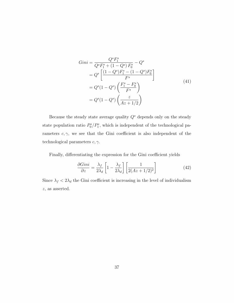
Because the steady state average quality Qs depends only on the steady

state population ratio P s0 /P

s1 , which is independent of the technological pa-

rameters c, γ, we see that the Gini coefficient is also independent of the

technological parameters c, γ.

Finally, differentiating the expression for the Gini coefficient yields

∂Gini

∂z=

λf2λd

[1− λf

2λd

] [1

2(Az + 1/2)2

](42)

Since λf < 2λd the Gini coefficient is increasing in the level of individualism

z, as asserted.

37