A Theoretical Analysis of AlternativeSchool Admission Rules

Gabrielle Fack∗

(Universitat Pompeu Fabra)

Julien Grenet*

(PSE)

November 2007

Abstract

In this paper, we construct a theoretical multi-community model of localpublic and private schools and housing markets with the objective of assessingthe analytical properties of various school school enrollment schemes (strictschool zoning, reassignment of school zones, open enrollment) on housingprices, residential and school social segregation and student performance inthe presence of peer effects. This theoretical framework allows for a preciseidentification of the channels through which the behavioral response of par-ents to different school enrollment policies might affect their housing locationand their decision to opt out of the public school system. This exercise alsopermits a quantification of the educational gains and losses incurred by pupilsin the different enrollment schemes, depending on their ability and parentalincome. To perform school enrollment policy simulations, the model is cal-ibrated using data on the city of Paris. Among other results, we show thatthe presence of private schools radically modifies the effectiveness of openenrollment or shifts in school attendance boundaries in reducing educationalinequalities.

JEL Classification H4, H7, I2

Keywords School enrollment; Location Choice; Peer Effects; Segregation

∗Paris School of Economics, 48 boulevard Jourdan, 75014 Paris, France. Email:gabrielle.fack@ens.fr et julien.grenet@ens.fr. We wish to thank Caroline Hoxby, Steve Machin,Thomas Nechyba, Thomas Piketty and Etienne Wasmer from their helpful comments and sugges-tions.

1

1 Introduction

The theoretical literature on public good provision and sorting into neighborhoods

has been growing since the seminal paper by Tiebout (1956). More recently, the

heated debate on school choice versus school zoning started a specific trend in the

literature that studies the link between school enrollment policies, residential segre-

gation and school stratification by pupil ability.

In this paper, we construct a theoretical multi-community model of local public

and private schools and housing markets with the objective of assessing the analytical

properties of various school enrollment schemes (strict school zoning, shifting of

school attendance boundaries, open enrollment) on housing prices, residential and

school social segregation as well as on student performance in the presence of peer

effects. This theoretical framework allows for a precise identification of the channels

through which the behavioral response of parents to different school enrollment

policies might affect their housing location and their decision to opt out of the

public school system. This exercise also permits a quantification of the educational

gains and losses incurred by pupils in the different enrollment schemes, depending

on their ability and parental income.

In order to calibrate the model and to perform school enrollment policy simu-

lations, we use the values of the parameters that we estimate in Fack and Grenet

(2008).

The remainder of this paper is organized as follows. In Section 2, we review

the theoretical literature on residential sorting and school enrollment policies1. The

next two sections are devoted to the presentation of our model. Section 3 presents

the simple case where all schools belong to the public sector. Private schools are

introduced in section 4. Section 5 presents the simulation results of alternative school

enrollment schemes. Finally, section 6 calibrates the model using the estimated

values of the key parameters in the Parisian case.

2 Review of literature: theoretical models of school

choice

In line with canonical models of local public finance, a strand of the literature has

focused on the quality of local public schools. Most models show that when schools

are financed locally, social inefficiencies may arise because of a sorting phenomenon.

1We do not to review the literature that studies other educational issues related to sorting,such as the papers by Benabou (1996a,b) and Fernandez and Rogerson (1998). These papersstudy the macroeconomic effects of educational systems in the presence of credit constraints andcomplementarities in productions, and compare systems of local public finance to State finance inthe long-run. For a review of this literature, see Fernandez (2003).

2

Fernandez and Rogerson (1996) study a multi-community model in which the

local public good is educational spending per pupil, which is financed through local

income tax. Households are heterogenous in income. In this model, both the level of

provision of school quality and the level of tax are affected by the composition of the

community, a feature that may lead to multiple equilibria. In this type of models,

imposing a single crossing condition on preferences is required to yield a unique

stable equilibrium, characterized by the stratification of households by income2.

A critical assumption: the single-crossing condition. As the single crossing

condition is imposed in the vast majority of models, let us write it more formally.

Typically, a simple multi-community model consists of a number of communities

that provide a local good q (such as school quality) at a local price p (either a

housing price or a local tax). Households choose where to reside depending on the

level of q and p. The utility function U(c, q) of a family is a function of a numeraire

good c (equal to the income minus the price of the local good p) and the local

public good q. U is assumed to be twice continuously differentiable and its partial

derivatives U1 and U2 with respect to c and q to be positive.

The single crossing condition assumes that the slope of the indifference curves

in the (q, p) space is everywhere increasing (or decreasing) in y:

∂(dpdq|u=u

)∂y

=∂(U2

U1

)∂y

=U21U1 − U11U2

(U2)2> 0 (1)

condition (1) ensures that if a household with income y0 weakly prefers the bundle

(pj, qj) offered in community j to the bundle (pk, qk) offered in community k where

pj > pk, then all households with income y > y0 also prefer (pj, qj) over (pk, qk),

as shown in figure 1. Alternatively, if a household with income y0 weakly prefers

(pk, qk) over (pj, qj), then all households with income y < y0 will also prefer (pk, qk)

over (pj, qj).

One might wonder how realistic is the single crossing condition. In the most

common form where households are heterogenous in income, this condition simply

states that the demand for school quality must be increasing with income, i.e. that

school quality is a normal good. When households are heterogenous in ability, the

condition implies that the demand for school quality is increasing with ability, which

might seem more controversial, as we discuss below3.

The single crossing condition is a very powerful assumption since it implies that

2Imposing a local stability condition ensures that the pooled equilibrium with all communitieshaving the same composition is not a stable equilibrium.

3In dynamic settings where education is modelled as an investment, it possible to get thesame sorting effects without imposing heterogeneity in preferences, by assuming imperfect creditmarkets. These types of models are reviewed in Fernandez (2003).

3

individuals have incentives to sort, and gives rise to stratified equilibria4. However,

Fernandez and Rogerson show that because of peer-group externalities, this equi-

librium is not necessarily Pareto-efficient. When a household chooses a community,

it does not consider the (positive or negative) effect of its choice on the community

peer group5.

The importance of peer effects. Models of local school finance in which school

quality is solely determined by per pupil spending are not entirely appropriate to

study school enrollment schemes within schools districts. In these models, equaliz-

ing educational spending across district would indeed suppress the stratification of

schools. In order to study the effect of school enrollment policies and in particular

the introduction of school choice, one might therefore wish to introduce peer effects

at the school level, since this assumption will result in stratification across schools

even when finance systems are centralized at the district level. With the introduc-

tion of peer effects, school quality may vary with the composition of the student

body. Peer effects play a crucial role in several models, including Benabou (1993,

1996a,b) and de Bartolome (1990), but we restrict our presentation to models that

focus on school zoning and school choice policies.

Modelling peer effects is a difficult task, as the empirical evidence is mixed on

this issue. While many empirical papers estimate a linear-in-means model and find

that pupils’ individual performance depends on the mean ability of their classmates,

recent empirical findings by Hoxby and Weingarth (2005) call into question the

linearity of peer effects6. Their results suggest that even if most pupils benefit from

having better peers, too much heterogeneity in the classroom can be detrimental.

The worst class composition seems to be the bimodal distribution, with a mix of low-

ability and high-ability children and no middle ability peers in-between. According

to their estimates, the most efficient class composition would be characterized by a

continuum of low to high achieving children without too much variance.

In existing multi-community models, the utility function of households typically

depends on the average pupil ability in the school. In one specification, Nechyba

(2003) allows for curriculum targeting (a lower variance in peer quality is assumed

4Fernandez (2003) stresses two other implications of the single crossing condition: first, itensures the existence of a majority voting equilibrium over the price p of the local public goodfor models with local taxes; second, it rules out the existence of pooling equilibria (in which allcommunities share the same composition) as long as a local stability condition is imposed.

5The inefficiency in Fernandez and Rogerson (1996) comes from the the additional assumptionthat the local tax rate voted by the median voter decreases when the mean income in the communityincreases. Under this assumption, moving some individuals with the lowest income from onecommunity to an adjacent community in which they become the richest group increases meanincome in both communities, decreases taxes and increases school quality, leaving everybody betteroff.

6See Hoxby and Weingarth (2005) for a critical discussion of the linear-in-means model and areview of alternative models of peer effects.

4

to improve the targeting of resources). Whether such information on school com-

position is available to parents and should enter their utility function is disputable.

If families only observe an overall measure of school quality that reflects the mean

of peers abilities, they can only rely on this information to make their choices. The

welfare effects, however, will critically depend on the form of peer effects.

School zoning and school choice. Epple and Romano (2003) develop a model

where families derive utility U(c, q, b) from a numeraire good c and their child’s ed-

ucational achievement which is itself a function of school quality q and the child’s

own ability b. School quality has two components: per student educational expen-

diture and the mean ability of the school peer group. In the benchmark case, school

admission is residence-based and families take school catchment areas into account

when choosing their home location. Education is centrally financed and a single

income tax rate is determined by majority voting. Epple and Romano show that if

income and ability are positively correlated, assuming that the demand for school

quality is normal (i.e. the single crossing condition is verified: Uq

Uyincreases with

y) and independent of ability (i.e. Uq

Uyis invariant with ability), then the model

generates a fully stratified equilibrium7 such that the wealthiest households live in

the community with the best schools and the higher housing prices8.

Introducing school choice radically modifies school composition, under the as-

sumption that schools face no capacity constraints and must admit all applicants.

As a result, school qualities are equalized, causing a decrease in housing prices.

This phenomenon yields an income effect that triggers an increase in educational

expenditures (through a higher tax rate). Compared to the school zoning case,

low-income families attend better schools whereas the effect is ambiguous for higher

income households, as they suffer from a decrease in the peer group quality but

benefit from an increase in educational expenditure. Simulations indicate that the

aggregate educational change due to a move from school zoning to choice is always

negative, once the fall in housing prices is taken into account. The introduction of

a fixed transportation cost for those who want to attend a school outside of their

neighborhood further reinforces this negative educational effect since in this case,

the poorest children are left behind in their local schools whereas the children from

the same neighborhoods but with more privileged socio-economic backgrounds pay

the cost of attending a better school, causing peer quality to fall everywhere.

This model is insightful but suffers from two main limitations. First, it describes

school choice in a fairly unrealistic way, as schools are assumed to have no capacity

constraints. Yet in reality, oversubscribed schools usually have the possibility of

7Epple and Romano show that stratified equilibria might also arise if ability is independent ofincome but the demand for school quality increases with ability.

8Other non fully stratified equilibria might exist but they are unstable under a reasonabledefinition of stability.

5

selecting their pupils. Second, it generates a very high level of stratification, which

is not what we observe in the data. This seems problematic for our purpose, since

our goal is to calibrate a model to study the effect of various school enrollment

schemes on school and residential stratification.

In order to yield more realistic levels of segregation in equilibrium, several mod-

els have introduced additional fixed attributes in the community, such as housing

quality (Nechyba, 1997) or school effectiveness (Rothstein, 2006). In these models,

incomplete stratification arises because choices are constrained by the fixed num-

ber of communities. The added richness of such models nevertheless comes with a

drawback in terms of tractability: if the existence of equilibria can be proved, they

can only be characterized through numerical simulations.

Models with additional community attributes. In a series of papers, Nechyba

(1997, 1999, 2000, 2003) developed and calibrated a general equilibrium model of

school finance that includes multiple school districts and multiple neighborhoods

within school districts. The purpose of these models is to study the effect of various

educational policies, such as finance equalization, State grants, school choice and

school vouchers. The features of Nechyba’s model exhibit three main differences

compared with the previously described general equilibrium models of school finance:

1. Wealth is determined endogenously, as households are initially endowed with

a house whose price is set in equilibrium. In addition, taxes are paid on

property instead of income. As a result, the single crossing condition is no

longer sufficient to ensure the existence of stratified equilibria9.

2. The housing stock is fixed, with an ex ante partition of districts into neighbor-

hoods of different qualities, and households have to move in order to adjust

their housing consumption. This assumption is crucial for the model to exhibit

an equilibrium.

3. Private schools are introduced in the model. They function as clubs of parents

who share the cost of the school equally and are free to choose their mem-

bers. As there is no fixed cost, private schools are only composed of single

income/peers types of households. On the contrary, public schools must admit

all pupils (subject to a residence requirement in the school zoning benchmark

case).

In the model, households care about the “quality” of the community, the quality

of their house (which is considered exogenous), the quality of the school attended

9As explained in Nechyba (1997), stratified equilibria are obtained by making assumptionsabout the equilibrium marginal willingness to pay, instead of initially ordering agents by increasingmarginal rates of substitution.

6

by their child and private consumption. As in Epple and Romano (2003), school

quality is assumed to be a function of per pupil spending and of the average peer

quality in the school10. Public schools are state or locally financed through income

or property taxes set by majority vote.

Nechyba (1997) proves the existence of an equilibrium, but simulations are

needed to characterize its properties11. In the benchmark equilibrium without pri-

vate schools, increased valuation of peer effects leads to greater residential stratifica-

tion of households based on income and wealth, more stratified property values and

more stratified school quality. When private schools are allowed to operate, they

tend to appear in low-income communities. A number of middle to high-income

households then decide to relocate in the high quality houses of low-income com-

munities in order to pay lower house prices and send their children to the newly

created private schools. As a result, private schools tend to lower the stratification

of income, wealth and property values. The creation of private schools in low-income

communities does not directly improve local public schools because they decrease

peer quality in the public schools by cream-skimming the best pupils. But since

the high-income parents who reside in these communities and send their children to

private schools also finance public education through property taxes, spending per

pupil increases in public schools. The net effect is ambiguous and varies with the

type of financing scheme adopted and the value of the calibration coefficients12.

The introduction of State-financed private school vouchers yields the same quali-

tative results, with higher income households opting out of public schools and moving

to high quality houses in lower quality neighborhoods where they send their children

to private schools. As long as the public support for public school remains above

the 50% threshold, per pupil public school spending in poor communities increases

as peer quality falls, with a net positive effect. However, the quality of public school

in the high-income neighborhoods unambiguously suffers from the introduction of

10In the earlier paper (Nechyba, 1999), peer effects are perfectly correlated with income but laterpapers allow for more sophisticated versions of peers effects.

11Practically, the computation of the equilibrium involves several steps, starting with the bench-mark case without private schools. Households are initially endowed with income and a house.They vote over property tax rates (if schools are locally financed) taking other characteristics(housing prices, school quality) as given. Given the tax rate, each household chooses its preferredlocation, then prices adjust and voting takes place again and so forth until the equilibrium isfound. Nechyba states that a unique equilibrium without private schools exists when preferencesare identical and communities sufficiently different in their inherent desirability. In the equilibriumwith private schools, parents first choose their preferred tuition levels taking other things (taxes,housing prices, school quality) as given, then choose wether they prefer to enroll their child in apublic or a private school. The vote over the tax rate then takes place, with households who havechosen private schools voting for a zero tax rate. Again, people choose simultaneously their homelocation and public/private school. This process is repeated until the equilibrium is reached.

12In Nechyba (1999), the latter effect dominates and results in an increase in the overall schoolquality. But in the calibration that replicates the New York mix of state and local finance (Nechyba,2000), public school quality falls because the decrease in peer quality is not offset by an increasein public school spending.

7

vouchers, as both peer quality and per pupil spending fall.

The case of state-funded public schools where per pupil spending is equalized

across districts (instead of locally financed schools), which is of great interest from

our perspective, yields pretty much the same results. As long as peer quality matters

to parents, state funding does not prevent substantial stratification of income to

arise in the benchmark equilibrium. However, the introduction of private schools and

private school vouchers yields much lower fiscal benefits for poorer districts, because

the increase in per pupil spending triggered by high-income households opting out

of the public school system is now spread across the entire State and no longer

concentrated in the poorest communities. Moreover, the pattern of relocation of

high-income households in low-income communities happens at a much lower pace

when school vouchers are introduced, since there are no incentives tied to lower

property tax rates when public education is state-funded.

For our purpose, the main predictions of such models are that the presence

of private schools and the introduction of school choice through the introduction

of vouchers decreases residence-based stratification and housing prices differentials

between neighborhoods, while it increases school-based stratification. Public schools

experience a decrease in peer quality that may not always be compensated by an

increase in per pupil spending. Nechyba points out that these results reflect very

“pessimistic” assumptions about the impact of school choice, since there are no

efficiency enhancing effect from the higher level of competition between public and

private schools. Introducing such effects yields an increase in public school quality as

private school attendance increases, which may offset the decrease in peer quality13.

Rothstein (2006) develops a model to test the strength of these efficiency en-

hancing effects. More precisely, the aim of his paper is to test whether parental

preferences depend primarily on school effectiveness or on school peers. This ques-

tion is related to the argument that school choice is the “tide that lifts all boats”14.

Advocates of school choice argue that increased school competition will give schools

the incentives to improve their efficiency, since parents value school effectiveness.

But if parents value peer groups more than school effectiveness (they may for ex-

ample prefer poorly run schools with high quality peer over more effective ones but

with a worse student body), then increasing school choice would not strengthen the

incentives for school management to improve school effectiveness.

These predictions are derived from a multi-community model where household

utility is a function of non-housing consumption (income minus housing rents) and

school quality. School quality in community j is a function of two parameters: peer

13Nechyba (2003) introduces two types of effects: curriculum targeting, implying that the lowerthe variance in peer quality, the better the targeting of resources, and competitive efficiency gains,which means that the marginal product of a dollar of spending rises in public schools when theyface greater competition.

14See Hoxby (2003).

8

group quality (measured by xj, the mean income of families living in community j)

and an exogenous school effectiveness factor µj:

qj = δxj + µj

The fact that parents care about composite school quality qj rather than about each

of its component drives the results of perfect sorting along qj, but not necessarily

perfect sorting along peer group quality and school effectiveness.

Provided that the single crossing condition holds, the rankings of communities

by quality, housing rents and average income are identical in equilibrium: the n

highest-income families live in the highest quality, highest rent community; the next

n families in the second highest-quality, second-highest-rent community, and so on.

If parents do not care about peers effects but only about school effectiveness (i.e.

δ = 0), there is a unique equilibrium which sorts families by effectiveness. But for

higher values of δ, other equilibria might arise, as shown in Rothstein’s simulations.

The model predicts that if parents do care about school effectiveness more than

school peers, then we should see perfect effectiveness/income sorting. Households

with higher income would therefore tend to locate in neighborhoods with betters

schools, both in term of peer group and effectiveness. However, if parents value peer

groups more than school effectiveness, there can be “unsorted” equilibria in which

communities with ineffective schools have the wealthiest families and are the most

preferred. These equilibria result from coordination failures, as no individual family

in the wealthiest neighborhood is willing to move alone to a district with a lower

peer group.

Simulations suggest that this problem is less severe when the number of district

is large, thus offering more choice to families. The difference in peer quality between

two “adjacent” communities is smaller in high choice districts, reducing the cost (in

terms of peer quality) of moving to the next lower peer group community if it is

endowed with a more efficient school. One testable prediction of this model is that

if parents have a moderate taste for school effectiveness, then effectiveness sorting

should be more complete in “high choice” cities (i.e. in areas with many small dis-

tricts) than in cities with little school choice. This prediction is tested empirically.

The estimates show no evidence of higher effectiveness sorting in high choice dis-

tricts. The most plausible explanation to this result is that that either parents place

a low weight on school effectiveness or they value it but lack information.

Our model builds principally on the model developed Nechyba, but simplifies

it and adapts it to the specific context of the French school system. In our model

as in Rothstein’s, we abstract from tax concerns and we do not look at schooling

expenditures, as the French system is centrally financed. We focus therefore only on

the peer effect component of school quality. But as we also want to derive predictions

on residential sorting, we build on Nechyba and assume that families not only care

9

about school quality, but also value neighborhood characteristics.

Finally, we wish to introduce private schools because they are well developed

in France and represent an outside option for many parents. Apart from Nechyba,

very few papers include private schools in multi-community settings. Epple and

Romano (1998) model sorting into private schools but without housing markets.

They show that when families differ both in terms of income and child ability, the

equilibrium composition of private schools may mix high-ability children from low-

income families with higher income but lower ability children15. This result comes

from the fact that private schools are able to internalize the externalities caused by

peer-effects by setting different fees for different levels of abilities. Martınez Mora

(2006) introduces choice between private and public schools along with residential

choice, but peers do not play any role as school quality is produced with a constant

return to scale production function. As we explain below, our goal is to take into

account peer-effects at the private school level and to model the specific features of

the French private school system.

3 Modelling alternative school enrollment schemes

In this section, we construct a multi-community model of school and residential

choice that allows us to compare two alternative school enrollment schemes. In the

first setting, the assignment of pupils to schools is purely residence-based while in

the second, parents can freely choose their child’s school. For now, all schools belong

to the public sector. Private schools will be introduced in section 4.

3.1 Strict school zoning

We first consider a setting in which pupil enrollment is based on a strict school

zoning scheme.

3.1.1 Assumptions

The city. As in Nechyba (1997) and Rothstein (2006), we assume that the city

consists of a continuum of families. In our model, families are points of a bounded

measurable subset C of the plane. Henceforth, the measure µ(A) of a measurable

subset A of C will be the Lebesgue measure (or area) of A. The city is partitioned into

K distinct neighborhoods {N1, ..., NK} that are assumed to be measurable subsets of

C satisfying µ(Nk) > 0 for any k = 1, ..., n. Each neighborhood is endowed with the

same measure of identical houses, owned by absentee landlords. Neighborhood k has

a positive specific quality qk, and we shall denote by q the corresponding bounded

15They assume that the creation of a private school entails a fixed cost, defining a minimum sizefor the private school.

10

measurable function which is constant and equal to qk on Nk. This specific quality

may include all the neighborhood amenities (architectural style, transportation fa-

cilities, parks...) except schools. The geographical distribution of these qualities is

not uniform, as quality is assumed to decrease with the distance to the city center16.

In the simulations, we assume that the logarithm of neighborhood quality ln (qk)

follows a distribution φ and that its rank is correlated with the rank of its proximity

to the city center (denoted rk( 1dk

), where 1dk

is the inverse of the distance to the city

center dk) with a positive correlation equal to λ.

School catchment areas. The city is partitioned into J middle school zones

{Z1, ..., ZJ} that are assumed to be measurable subsets of C, such that µ(Zj) > 0

for any j = 1, ..., J . The boundaries of school catchment areas do not necessarily

coincide with neighborhoods’ borders and some school zones may overlap several

neighborhoods. Initially, the assignment of pupils to schools is strictly residence-

based: a pupil living in a specific catchment area must attend the local school. The

size of schools is therefore equal to the number of children (one per household) living

within the corresponding attendance zone.

The subsets Bjk = Zj∩Nk of C are called blocks. We will only consider the pairs

(j, k) ∈ {1, 2, ..., J} × {1, 2, ..., K} such that µ(Bjk) > 0.

As the French system is centrally financed, we assume that school spending does

not play any role: spending per pupil is the same across schools17 and schools are

equally efficient in the use of their funds. We therefore abstract from tax and voting

concerns to focus our analysis on peer effects. As a result, families care about the

average ability of children enrolled in the school, because it is the only factor that

drives variations in school performance. We assume that a child benefits from higher

ability peers in the school. Educational achievement ei of pupil i is a linear function

of her own log ability ln ai and of the average level of log ability in her school j (Sjdenoting the subset of families whose children are assigned to school j):

eij = ln (ai) + δ

∫Sj

ln (ai)dµi (2)

Our specification in natural logarithm reflects the fact that even though scores

are usually normally distributed, it is not necessarily the case that abilities follow

the same distribution. In fact, a log-normal distribution of abilities sounds more

plausible, since earnings are log-normally distributed. Our interpretation is that the

grading of tests maps log-normal distributions of abilities into normal distributions

16To replicate Parisian features, we suppose that quality decreases as we move away from thecity center.

17We therefore do not have to include the within-neighborhood voting over public school spend-ing, which is a central feature of many multi-community models.

11

of test scores18. We assume that parents only observe test scores, which themselves

reflect the log of abilities. The average test score at the school level can be written:

ej = (1 + δ)

∫Sj

ln (ai)dµi (3)

Our specification of peer effects implies that a point increase in the average test

score raises a pupil’s own achievement by δ1+δ

. This coefficient may therefore be

easily related to empirical estimates of peer effects based on test score data.

It is important to note that given our linear specification of peer effects, school

choice reforms that modify the composition of schools will not yield aggregate educa-

tional gains. This specification allows us to restrict our analysis on the distribution

of gains and losses induced by different school enrollment policies.

Families. Families living in the city are endowed with an exogenous level of in-

come. We denote by yi = y(i) the income of family i ∈ C and by y the corresponding

f income function. Each family must rent a house to live in the city and we assume

that the number of houses is equal to the number of families. Every family i has

a child of middle school age, with school ability ai = a(i) and we shall denote by

a the corresponding function. Families only differ in their income yi and in their

child’s ability ai. These two variables y, a : I → R+ are assumed to be bounded (and

measurable). They are not independent and we will assume that their correlation

coefficient ρ is strictly positive.

The utility enjoyed by family i is a function of two key parameters that will jointly

determine its residential choice: private consumption ci and the desirability hjk of

its house located in school zone j and neighborhood k (i.e. block Bjk). The utility

function Uijk = U(ci, hjk) is assumed to be twice continuously differentiable and U1

and U2 (the partial derivatives with respect to the first and second argument) are

both positive. Household private consumption ci is what is left after the payment

of the rent pjk.

The desirability hjk of a house is weighted average of two parameters:

1. the quality qk of the neighborhood k;

2. the perceived quality of the local middle school j, which is measured by the

average logarithm of abilities in this school.

More precisely, we set:

hjk = β

∫Sj

ln (ai)dµi + (1− β) ln(qk) (4)

18For example, it is well-known that the IQ tests are designed to yield a normal distribution ofscores.

12

with 0 < β < 1.

If we assume that parents do not really observe the average logarithm of abilities

in the middle school but instead only know the average test score results ej, then the

parameter β which measures the taste for school quality includes peer effects. In this

case, we can rewrite the block’s desirability as a function of average achievement:

hjk =β

(1 + δ)(ej) + (1− β) ln(qk) (5)

Key assumptions on the utility function. We make two important assump-

tions about households’ utility function.

H1: Single crossing condition First, we make the usual assumption that

the utility function satisfies the single crossing condition:

U12U1 − U11U2 > 0

This condition simply states that demand for desirable housing is normal. As

we will see below, this condition ensures that any residential equilibrium will be

perfectly stratified on the basis of household income (highest-income families will

live in the highest desirable neighborhood, and so on). However, it does not imply

perfect stratification on school or neighborhood quality, and does not rule out the

possibility of multiple equilibria.

H2: Demand for desirability is invariant to its level. In addition, we

make the following assumption:

U22U1 − U12U2 = 0

which ensures that:∂(U2

U1

)∂h

=U22U1 − U12U2

(U1)2= 0

This condition states that the demand for a desirable house is invariant to its

level. It is needed for an equilibrium to emerge when families are free to choose the

school they which to send their child to. This condition ensures that two families

with the same income y0 but children of different abilities will have the same demand

for housing desirability.

The family of functions that satisfy these two assumptions has the form:

U(c, h) = W(V (c) + h

)

13

with V a C2 strictly increasing concave function and W a C2 strictly increasing

function.

Let us now prove more formally, with this form of utility functions, the stratifi-

cation property implied by the single crossing condition.

Lemma: Suppose that hjk > hj′k′ , pjk > pj′k′ and that utility function are of the

above form. Then we have:

(i) If a family with income y0 (weakly) prefers block (j, k) to block (j′, k′), then

all families with income y > y0 will strictly prefer block (j, k) to block (j′, k′).

(ii) If a family with income y0 (weakly) prefers block (j′, k′) to block (j, k), then

all families with income y < y0 will strictly prefer block (j′, k′) to block (j, k).

Proof:

(i) By hypothesis, we have W(V (y0− pjk) +hjk

)≥ W

(V (y0− pj′k′) +hj′k′

)and

hence, since W is strictly increasing:

V (y0 − pjk) + hjk ≥ V (y0 − pj′k′) + hj′k′

So, we get:

V (y0 − pj′k′)− V (y0 − pjk) =

∫ y0−pj′k′

y0−pjk

V ′(t)dt ≤ hjk − hj′k′ (6)

Since V ′ > 0 and V ′′ < 0, V ′ is a strictly decreasing positive function. We

thus get, for any y > y0:

V (y−pj′k′)−V (y−pjk) =

∫ y−pj′k′

y−pjk

V ′(t)dt <

∫ y0−pj′k′

y0−pjk

V ′(t)dt ≤ hjk−hj′k′ (7)

and the proof of (i) is complete.

(ii) The proof is analogous to the proof of (i).

Remark 1. Note that the condition (ii) still holds if we only have pjk > pj′k′ ,

provided we assume that the family with income y0 strongly prefers block (j′, k′) to

block (j, k). We shall use this remark later to show the stratification properties of

all equilibria.

14

Housing prices. In this model where families are competing for houses, we make

the assumption that the price of houses is fixed by landlords. Let us denote by

p : C → R+ the price function which is assumed to be constant on each block Bij.

Family decision problem. Families are utility maximizing agents that choose

location (j, k) while taking public school quality and housing prices as given. Fam-

ily i chooses its location among all feasible locations in the budget set determined

by the constraint yi ≥ pj,k.

School zoning equilibrium

An equilibrium is defined by a set of housing prices and a partition of families

into bins Cj,k. Given the spatial layout of school zones and neighborhoods, the

distribution of neighborhood qualities, income and pupil abilities, families have a

housing preference for each block Bjk that must satisfy the following conditions:

1. Each family has a house: µ(Bjk) = µ(Cjk) for any pair (j, k).

2. Nash equilibrium: at the specified housing prices, no family would prefer

a house other than the one to which she has been allocated, given the set of

affordable locations:

U(yi − pjk, hjk) > U(yi − pj′k′ , hj′k′) ∀i, j, k

where

hjk = β

∫∪kCjk

ln (ai)dµi + (1− β) ln(qk)

Our model of strict school zoning describes an economy that is a simplified

version of the economy described in Nechyba (1999). It simply abstracts from tax

concerns, property wealth and private schools. Nechyba’s proof of the existence of

an equilibrium (Nechyba, 1999) applies to our model.

As household wealth is exogenous in our model, the single crossing condition

implies that the equilibrium is stratified. We will use this property to construct an

algorithm that converges rapidly to the equilibrium.

Proposition. In equilibrium, we have, for any pair (j, k) 6= (j′, k′):

(i) If hjk > hj′k′ (respectively hjk > hj′k′), then pjk > pj′k′ (respectively pjk > pj′k′).

(ii) If family i lives in Bjk and family i′ lives in Bj′k′ and if yi > yi′ , then hjk > hj′k′

and pjk > pj′k′ .

15

Proof. Let us prove this proposition.

(i) Assume that hjk > hj′k′ . To prove that pjk > pj′k′ , we use a proof by con-

tradiction. Assume that pjk < pj′k′ . Then, any household i who can afford a

house in Bj′k′ can also afford a house in Bj′k′ since we have yi > pj′k′ > pjk.

Since U is strictly increasing in both arguments, we get from the inequalities

yi − pj′k′ < yi − pjk and hj′k′ 6 hjk the following inequality:

U(yi − pj′k′ , hj′k′) < U(yi − pjk, hjk)

But we have in equilibrium that for any family i living in Bj′k′ :

U(yi − pj′k′ , hj′k′) > U(yi − pjk, hjk)

which leads to a contradiction. This shows that pjk > pj′k′ . The case of strict

inequality is demonstrated in a similar fashion, so (i) is proved.

(ii) Consider a family i living in Bjk, a family i′ living in Bj′k′ and assume that

yi > yi′ . We have yi > pjk, yi′ > pj′k′ and since yi > yi′ , we get yi > pj′k′ . In

particular, family i can afford to by a house in block Bj′k′ . Since we are in

equilibrium, we have:

U(yi − pjk, hjk) > U(yi − pj′k′ , hj′k′) (8)

Let us prove by contradiction that we must have hjk > hj′k′ . If hjk < hj′k′ , we

would get pjk > pj′k′ by property (i). By remark 1 (see above), we would then

write (using equation (8):

U(y − pjk, hjk) > U(y − pj′k′ , hj′k′)

for any y < yi, and hence, for y = yi′ :

U(yi′ − pjk, hjk) > U(yi′ − pj′k′ , hj′k′)

But this contradicts the relation:

U(yi′ − pj′k′ , hj′k′) > U(yi′ − pjk, hjk)

which follows from the fact that we are in equilibrium. Since we get a con-

tradiction, we have proved that hjk > hj′k′ . The relation pjk > pj′k′ follows

from (i).

This proposition ensures that the equilibrium will be perfectly stratified by in-

come. The equilibrium allocation of families to blocks is generally not unique be-

16

cause the quality of neighborhoods within a particular school zone might be het-

erogenous. However, the simulations that we perform in section 5 to compare the

properties of alternative school enrollment policies are based on an algorithm that

always converges to a unique equilibrium for a given initial geographical distribution

of households.

3.2 School choice

So far, we have assumed that a strict school zoning policy is enforced by the local

education authority. We now examine what happens if we introduce school choice.

Ranking of schools under school choice

We model school choice as follows. A family is free to apply to any school and to

move from one school to another as long as the school principal is willing to enroll

the child. Total enrollment cannot exceed a school’s capacity which is assumed to be

equal across schools. Any transportation cost paid to attend a school located outside

the district is publicly funded so the location of middle schools no longer matters.

Families have identical preferences over schools: they care about average test scores,

so all of them would prefer sending their child to the school which enrolls the most

able pupils. For a given distribution of average abilities across establishments, the

ranking of schools will be identical for all families.

The school choice allocation rule. We assume that the objective of school

principals is to maximize their establishments’ performance. The optimal strategy

is therefore to enroll children with the highest abilities. For the moment, we assume

that a school principal can freely choose the student body, and therefore selects the

mth highest ability pupils among applicants. The allocation process will typically

involve several rounds, the principal being allowed to turn down an application to

accept instead a pupil with higher ability.

School choice equilibrium. An equilibrium is reached when all children are

enrolled in a school and when no family can find a preferred school in which its

child could be enrolled instead. In equilibrium, the highest ability children will be

allocated to their preferred schools and lower ability children would not be admitted

to that school by the principal. Schools are therefore perfectly stratified by ability:

the children that compose the student body of the jth preferred school (1 6 j 6 J)

have an ability comprised in the interval [aj, aj].

In this set-up, the quality Γ(j) of the jth preferred school is higher than the

17

quality of all schools j′ such that j′ < j and can be written:

Γ(j) = ln(a)j

=

∫Aj

ln(ai)dµi (9)

where Aj is the set of all pupils whose ability ai lies in the interval [aj, aj].

Residential equilibrium

The residential equilibrium is defined in the same way as in the residence-based

assignment setting, but the equilibrium that emerged under strict school zoning

will not in general be an equilibrium under the new school choice scheme. In the

strict school zoning scheme, households are sorted on the basis of the desirability

of blocks, which is itself a function of both neighborhood quality and local public

school quality.

When school choice is introduced, local public school quality no longer matters

for family i and is replaced in its utility function by the quality of the “chosen”

public school, ln(a)j. Note that all blocks within a given neighborhood k are now

strictly equivalent from the point of view of parents, so we drop the subscript j and

denote by Bk all blocks of this neighborhood and by hk the common desirability of

the houses located within these blocks.

The stratified equilibrium. The single crossing condition defined over the de-

sirability of block k is no longer sufficient to ensure that the stratified equilibrium is

a Nash equilibrium. We need to show that at the specified housing prices and given

the current distribution of income across neighborhoods and the current distribution

of abilities across schools, no family would prefer to live in a district other than the

one in which it currently resides:

U(yi − pk, h(ai, qk)

)> U

(yi − pk′ , h(ai, qk′)

)∀i, k, k′

If we assume that qk > qk′ and pk > pk′ , the single crossing condition ensures that

if a family with income y0 and child ability a0 weakly prefers block k to block k′, then

a family with higher income but identical child ability will strictly prefer block k.

The proof is similar to the one given in the strict school zoning setting.

But as abilities are not perfectly correlated with income, the single crossing

condition does not guarantee that a family with the same income y0 but different

child ability (a1 6= a0) also strictly prefers block k to block k′. Assumption H2

ensures that this holds (the proof is straightforward given the family of functions

defined above).

Under these two conditions, a stratified equilibrium exists with higher income

households living in the more desirable neighborhoods (in terms of intrinsic qual-

18

ity q). As neighborhood qualities are assumed exogenous, this equilibrium is unique.

School quality is no longer capitalized in housing prices that are determined uniquely

by differences in neighborhood qualities.

4 Introducing private schools

We have assumed so far that the only available schools are public schools. This

assumption is very unrealistic, in particular in the French case, where private schools

account for about 20% of total middle school enrollment (the proportion going up

to 30% in Paris). Yet modelling private school in the presence of peer effects if not

a straightforward task. In the existing literature, Nechyba (followed by Ferreyra,

2007) is the only author to introduce private schools with peer effects in a housing

market model. However, he ensures that peer quality is unique for every child by

assuming that the creation of a private school does not require any fixed investment,

so the size of a particular private school could be equal to one student. As a result,

every private schools enrol only pupils that share the same income and ability. In

this set-up, a family willing to opt out from the public school system always has the

possibility of sending its child to a private school with a peer group that matches

its child’s ability.

Because many features of the French education system would not be well repro-

duced under such assumptions, We decided to model private schools in a way that

seems more appropriate.

Some stylized facts about private schools in France. The specific features

of the French private school system are detailed in Fack and Grenet (2008). Three

main specificities are worth emphasising here:

• Private schools can freely select their pupils. As a result, the average perfor-

mance of private schools is usually higher than that of public schools.

• Private school fees are much smaller that in the US or the UK, because the vast

majority of public middle schools receive public funding which covers teachers’

pay and most equipment expenses. For simplicity, we will assume that there

are no private schools fees.

• As private schools are usually State-funded, the opening of new schools is

subject to very tight restrictions19. The size (and growth) of the private school

sector is therefore limited. More precisely, public subsidies to private schools

depend on the approval of a commission (composed of members of public

19In France, although opening a private school is relatively easy, it is much more difficult to getpublic funding. As a result, the number of non-subsidized private middle schools (Hors contrat) isvery small and can be neglected.

19

administration, representatives of local communities and representatives of

private schools) and must meet a “recognized need for education” (besoin

scolaire reconnu)20.

In a strict school zoning scheme, private schools offer an outside option to parents

that are unwilling to send their child to the local public school. However, as the size

of the private sector is restricted, private schools cannot completely replace public

schools, as is the case in Nechyba (1999) or Epple and Romano (1998), where private

schools are costless. If the size of the private sector was unrestricted, we would end

up with an equilibrium similar to the school choice equilibrium, with private schools

fully replacing public schools.

Private schools as local clubs. In our model, private schools function as local

clubs but we assume that there is an implicit fixed cost to create a private school

and a maximum public subsidy such that the size of a private school corresponds to

a neighborhood (assuming that all children living in the neighborhood attend the

private school). For simplicity, we do not model the cost of setting up a private school

since in France, this cost is usually not incurred by parents of children enrolled in the

private sector. However, if private schools were costless and if no restrictions were

imposed on the number of private schools operating in a city, they would completely

replace public schools and be perfectly stratified by parental income.

In order to model the restrictions that apply to private schooling in France,

we need to define a rule for the creation of private schools. As publicly funded

private schools can only be created if they meet a “recognized educational need”,

we assume that private schools will appear in neighborhoods where parents are the

most dissatisfied with the quality of the public school. We suppose that parents

living in the same neighborhood can form a coalition to set up a private school and

opt out from public education. This coalition is sustainable if the quality of this

prospective private school is high enough compared to the quality of the assigned

public school. For each neighborhood, we define a “will to secede” sk from the public

school as the difference between the quality of the private school ln (a)k

that could

be created in the neighborhood (assuming that all children in the neighborhood

attend the private school) and the quality of the local public middle school ln (a)j:

sk = ln (a)k− ln (a)

j(10)

If a neighborhood k is included in several school zones, the will to secede is the

weighted average will to secede in the neighborhood:

sk = ln (a)k−∑j

µ(Bjk)

µ(Nk)ln (a)

j(11)

20see art. L442-5 to L442-11 of the Code de l’Education.

20

where µ(Bjk) is the measure of the fraction of neighborhood k that is assigned to

public school j and µ(Nk) is the total measure of neighborhood k.

We assume that parents with the highest will to secede sk are willing to spend

more time lobbying members of the commission for private schools. As a result, only

neighborhoods with a sk superior or equal to a specific exogenous threshold s0 will

be allowed to create a private school. We assume that the private school never turns

down the application of children that live in the neighborhood. As all the children

in the neighborhood prefer the private school to the public school, it is not possible

for a child outside the neighborhood to enter the private school, given the capacity

constraints. These assumptions ensure that private schools do not entirely cream

skim public schools. Otherwise, we would end up with only the pupils belonging to

the top percentiles of ability attending private schools. Our model is closer to what

is observed in reality: private schools are on average better than public schools but

some public schools rank higher than private schools.

Private schools in a model of school zoning. We first establish the equilibrium

that emerges in the absence of private schools when the assignment of pupils to public

schools is strictly residence-based, and then investigate the effect of introducing

private schools in a dynamic setting. The introduction of private schools is therefore

dependant on the previous equilibrium and we perform simulations to reach the new

one. We do not formally prove the existence of an equilibrium with private schools

but our simulations suggest that we can always find one. The creation of a private

school changes the valuation of the neighborhood where it is located, since private

school quality is always better than that of the local public school. The desirability

of a neighborhood in which a private school operates therefore becomes:

hjk = β(ln (a)k) + (1− β) ln(qk) (12)

Where ln (a)k

denotes the average performance in the neighborhood’s private

school and qk is the neighborhood’s intrinsic quality. Note that the housing price

differential between two parts of the same neighborhood assigned to different public

schools disappears if a private school is created in the area, as the two parts of the

neighborhoods now share the same desirability.

In our simulations, if a private school created in a neighborhood in period t

becomes unsustainable in period t + 1 because of the lower average ability of the

new residents that have moved to the neighborhood, then the private school should

close. In fact, the simulations show that under reasonable values of the parameters,

this situation never happens. Once a private school is created, the quality of the

neighborhood increases relatively to other neighborhoods while the quality of the

public school in the area decreases, lowering the rank of surrounding neighborhoods.

This leads in equilibrium to an increase in the average income of neighborhoods that

21

have shifted to private schooling and a decrease in surrounding areas.

Private schools and school choice. Under the model’s assumptions, private

schools tend to disappear when school choice is introduced, because it becomes

almost impossible to find a neighborhood in which all families are willing to support

a private school instead of sending their child to the public school of their choice.

If a family has a child with high-ability, it would prefer sending her to the best

public school instead of the private school, causing a failure in the support for

the private school. As a result, private schools might only subsist in the top income

neighborhoods, if the average ability of peers is high enough compared with the best

public school. This could happen if the size of the neighborhood is small enough

compared to the size of public schools and if the correlation between income and

ability is very high. However, our simulation show that the occurrence of such a

scenario is rare enough to be neglected for credible values of the parameters.

5 Simulations

In this section, we use our model to perform simulations of alternative school en-

rollment schemes (both without and with private schools) for different values of

the parameters. Our goal is to predict the effect of various policies that have been

debated in France. We start with the analysis of the benchmark equilibrium of

strict school zoning, which corresponds to the existing situation in Paris. We then

analyze the impact of redesigning school catchment areas on school and residen-

tial social segregation and characterize the educational gains and losses incurred by

pupils depending on their ability and family income. Finally, we assess the effect of

switching from school zoning to school choice.

5.1 Simulations set-up

City and school catchment areas. In order to perform our simulations, we

represent the city as a checkerboard constructed as follows (cf. figure 2):

• The city has K = 100 neighborhoods and J = 16 school zones.

• Each school zone is composed of blocks belonging to 4 neighborhoods that

are entirely assigned to that particular school, 4 neighborhoods that overlap

2 school zones and 1 neighborhood that overlaps 4 school zones; the total

number of different combinations of school zones and neighborhoods is equal

to 144.

• The checkerboard is divided into 400 elementary cells of the same size, allowing

us to define the relevant income bins to simulate the allocation of households

22

to houses. The 144 combinations of neighborhoods and school zones have three

different sizes: they may contain 1,2 or 4 elementary cells depending of the

particular overlapping of neighborhoods and school zones. Figure 3 shows the

precise layout of cells, blocks and neighborhoods in four typical school zones.

The quality of each neighborhood is randomly picked up from a standard log-

normal distribution. The rank of a neighborhood’s quality is positively correlated

with the rank of the neighborhood’s proximity to the city center, with the correlation

coefficient being equal to λ.

Families. The total number of families is set equal to 10 000. Income and abilities

are picked up from a bivariate standard log-normal distribution with a correlation

coefficient equal to ρ: (yiai

)∼ N

[(0

0

),

(1 ρ

ρ 1

)]The utility function has the following specification:

U(ci, hjk) = α ln (ci) + hjk

where ci is the private consumption of family i and hjk is the desirability of the

block Bjk in which it resides.

Parameters of the model. The model has four parameters:

• ρ: the correlation coefficient between family income and child ability.

• λ: the correlation coefficient between neighborhood quality and the proximity

to the city center.

• β: the taste for school quality, i.e. the weight on school quality ln aj

in the

total desirability hjk of block Bjk, relatively to the weight on the exogenous

quality qk of neighborhood k.

• s0: the secession threshold for the creation of a private school. In order for

a private school to appear, the desirability to secede sk of families living in

neighborhood k must be superior or equal to s0.

5.2 Alternative school admission rules

Before explaining the simulation procedure, we need to define precisely the school

enrollment policies that we want to analyze and specify the main outcomes of inter-

est. We focus on the segregation outcomes and on the distribution of educational

23

gains and losses incurred by pupils from these policies. In addition, we investigate

changes in school stratification that arise when private schools are introduced in the

model.

Three alternative school enrollment schemes. We start with a benchmark

equilibrium of strict school zoning where each child is assigned to a school on the

basis of her address of residence.

Departing from this equilibrium, we then implement school zone reassign-

ments. This policy consists in redesigning school catchment areas in order to

change the composition of schools. We simulate a reassignment scheme that ini-

tially reduces stratification by abilities in all schools. Figure 4 shows how bound-

aries will be redrawn in our simulations. The original square-shaped zones are

changed to slice-shaped zones radiating from the city center. Given the correlation

between neighborhood quality and proximity to the center, this particular form of

reassignment tends to homogenize school zones in terms of the intrinsic quality of

neighborhoods.

Finally, departing from the strict school zoning equilibrium, we simulate the

impact of implementing open enrollment. This policy consists in allowing parents

to apply to the public school of their choice. Given our assumption that school

principals have the right to choose their students and seek to maximize the average

ability in their school, the resulting schooling equilibrium is completely stratified

by ability. This assumption reflects the empirical evidence on school choice when

no specific admission rules are imposed. For instance, Hsieh and Urquiola (2006)

find that the development of a voucher program in Chile yielded an increase in

ability stratification, with higher ability children leaving the public schools for the

private sector. However, school choice policies could be designed to restrict this

type of stratification effects, by introducing admission rules in the form of lotteries

for oversubscribed schools or specific admission criteria (preference given to children

with low parental income or living closest to the school, etc.). We do not investigate

these possibilities in our simulations and stick to a “cream skimming” version of

school choice. Similarly, we do not model potential efficiency gains that could arise

from increased competition among schools, as evidence on the subject is mixed21.

Segregation outcomes. Changes in school policies will affect both residential

and educational segregation. In our simulations, we consider two measures of seg-

regation:

21In a much debated paper, Hoxby (2000) uses natural boundaries such as rivers to identifyexogenous variations in choice and shows that cities which have a larger number of school districtsalso have more productive schools. However, Rothstein (2006) calls into question the existence ofsuch effects after replicating Hoxby’s estimations.

24

• Residential segregation: we measure residential segregation at the school

zone level by computing the ratio of the variance of the school-level average

log income over the total variance of log income in the city population:

Segres =Var(ln y

j)

Var(ln yi)

The higher the ratio, the higher the residential segregation between school

zones (the coefficient is equal to zero when there is no segregation).

• School segregation: we measure educational segregation across schools by

computing the ratio of the variance of the school-level average log ability over

the total variance of log ability in the population:

Segab =Var(ln a

j)

Var(ln ai)

The interpretation of this ratio is similar to that of residential segregation.

Distributional analysis of educational gains and losses. Under the assump-

tion that peer effects are linear in means, changes in school policies will have no effect

on aggregate educational achievement. However, alternative school enrollment poli-

cies are likely to affect pupils differently depending on their parental income and

individual ability. We therefore focus on the distribution of educational gains and

losses along these two dimensions.

The welfare implications of school enrollment policies are not limited to these

educational effects, since housing prices are also affected by the reforms. In a context

of local funding of schools through income or property taxes, it would be important

to take into account the wealth effects of school policies that arise through changes

in voting over school spending (see Epple and Romano, 2003). However, as our

model does not include educational spending as an input in the school production

function (the French school system being centrally financed), we abstract from these

other welfare effects and concentrate exclusively on peer effects.

More precisely, we use two measures of educational gains:

• The average peer ability change by decile of ability and income: The

individual gain (or loss) induced by a school enrollment policy change for a

given child is denoted ∆i and is equal to the difference between the average

log ability in the school j′ she attends after the implementation of the new

policy and that of the school j she was previously assigned to:

∆i = ln (a)j′

− ln (a)j

25

The average peer group change by decile of ability and income is computed as

the average ∆i for all children.

• The proportion of “winners” by decile of ability and income: we

compute the proportion of net “winners” in each decile of ability and income.

A child will win (respectively lose) from a school enrollment policy change if

the average ability of her schoolmates increases (respectively decreases). Note

that the proportion of winners is not necessarily equal to 1/2, since the size

of the effects can be asymmetric. For example, the average proportion can be

inferior to 1/2 if a small fraction of high-ability children becomes concentrated

in a school as a result of the policy, leaving all children in the other schools

worse off.

Educational gains are computed taking the initial school zoning equilibrium (with

and without private schools) as the reference point. We do not specify a social choice

function, but the two above measures of educational gains give an idea of the relative

weight that should be put on low-income children if one wanted to favor this group

when choosing among several policies, knowing that the net gains over the whole

population of pupils are zero because of the linear-in-means specification of peer

effects.

Specific outcomes for private schools. In order to study how the introduction

of private schools affects our results, we compute three additional indexes:

• the percentage of children attending private schools;

• the difference in the log average ability of children in public and

private schools;

• the segregation by ability within both public and private schools.

These outcomes are useful to assess the extent to which private schools cream-

skim the best students from public schools.

5.3 The simulation algorithm

In order to estimate the impact of various school zoning policies, we perform a series

of simulations using different sets of values for the parameters of interest. Residential

choice and the allocation of pupils to the various schools in equilibrium is computed

using an algorithm22 that consists of several steps and loops. An important feature

of our algorithm is that it does not move each of the 10 000 households but works on

elementary cells. We use the equilibrium property that households must be perfectly

22We coded the algorithm using SAS.

26

stratified by income to group them into 400 income bins corresponding to the 400

elementary cells. Each cell is represented by an average income and average ability,

with perfect ranking along these two dimensions. All the households belonging to

a given cell will therefore always be moved together. Another important feature of

the algorithm is that we do not need to calculate housing prices. Since the single

crossing condition ensures that higher income households will always pay higher

housing prices for blocks of higher desirability, we directly allocate households/cells

according to the ranking of the desirability of blocks.

No private schools

Benchmark equilibrium: strict school zoning with no private schools

(SZN). The algorithm proceeds as follows:

• Step SZN1: We simulate 10 000 households characterized by parental income

and child ability. The values of both characteristics are taken from a bivariate

standard log-normal distribution, with a correlation coefficient equal to ρ.

• Step SZN2: We simulate 100 neighborhoods, randomly distributed throughout

the city, under the constraint that the correlation between the rank of their

intrinsic quality and the rank of their distance to the city center is equal to λ.

• Step SZN3: The initial allocation of households is the one that would arise in

the absence of school zoning. Households are grouped into 400 income bins and

are allocated to the different neighborhoods so that the ranking of income bins

matches the ranking of the intrinsic quality of these neighborhoods. Note that

this initial allocation will determine the equilibrium allocation: a different

initial spatial allocation of households would yield a different allocation in

equilibrium. However, our choice for the initial allocation can be justified as a

starting point, since it corresponds to the equilibrium that arises when there

are no school zones.

• Step SZN4: Square-shaped school zones are defined, each one grouping a total

of 25 elementary cells. The initial allocation of households to the different

neighborhoods yields a school quality for every school zone (calculated as the

average log ability of pupils residing in the school’s catchment area). The

exogenous intrinsic quality of neighborhoods and the endogenous quality of

schools give rise to a unique ranking for the desirability of the 400 elementary

cells, for a given value of parameter β (the taste for school quality).

• Loop SZN: The 400 income bins are reallocated to the different cells so that the

ranking of income bins matches the ranking of elementary cell desirability. This

again modifies the quality of schools, initiating a new reallocation of income

27

bins to the various cells. The process is repeated until it converges to an

equilibrium. An equilibrium is reached when the spatial allocation of income

bins in period t is the same as the previous period’s allocation. Depending on

the values of the different parameters, an equilibrium is obtained within 10 to

20 successive iterations.

School zone reassignment with no private schools (SRN). The equilibrium

obtained under strict school zoning with no private schools (SZN) serves as the start-

ing point for the simulation of school zone reassignment. The algorithm proceeds

as follows:

• Step SRN1: The initial allocation of income bins on the checkerboard is the

one obtained in equilibrium under strict school zoning, for given values of the

parameters λ, ρ, β and an initial spatial allocation of neighborhood quality

throughout the city. The initial square-shaped school zones are replaced by

new slice-shaped ones. The initial allocation of income bins defines the initial

quality of these newly created school zones, which together with the neighbor-

hood intrinsic qualities defines the new desirability of the various cells.

• Loop SRN: The 400 income bins are then reallocated to the different cells until

an equilibrium is found, following the same process as in loop SZN.

Open enrollment with no private schools (OEN). The equilibrium obtained

under strict school zoning with no private schools (SZN) serves as the starting point

for the simulation of open enrollment. The algorithm proceeds as follows:

• Step OEN1: The initial allocation of income bins on the checkerboard is the

one obtained in equilibrium under strict school zoning, for given values of

the parameters λ, ρ and β and an initial allocation of neighborhood quality

throughout the city. School zones are then suppressed and replaced by open

enrollment. Under that scheme, pupils are univocally allocated to the various

public schools on the basis of their ability. Hence, in equilibrium, each school

enrolls pupils belonging to a same bin of ability.

• Step OEN2: under the assumption that demand for desirability is invariant to

its level (see subsection 3.1.1), the equilibrium allocation of households to the

various cells under open enrollment is identical to the equilibrium obtained

under strict school zoning when the parameter β (the taste for school quality)

is set to 0. In equilibrium, households are thus allocated to the different

neighborhoods so that the ranking of income bins matches the ranking of the

intrinsic quality of neighborhoods.

28

Introducing private schools

The three equilibria defined above (strict school zoning, school zone reassignment

and open enrollment) are extended to account for the endogenous emergence of

private schools. Residential choice and the allocation of pupils to public and private

schools in equilibrium is then computed using an algorithm that involves several

nested loops.

In our model (strict school zoning and school zone reassignment), private schools

consist of local clubs formed by parents at the neighborhood level. In order for a

private school to be created, it must be the case that the average difference between

the log ability of the pupils residing in a given neighborhood and the average log

ability in the surrounding public schools is higher than an exogenously predeter-

mined threshold s0. The way private schools appear and disappear is described

below.

Strict school zoning with private schools (SZP). The algorithm that ac-

counts for the introduction of private schools in the strict school zoning scheme

proceeds as follows:

• Steps SZP1 to SZP3 are identical to steps SZN1 to SZN3.

• Step SZP4: Square-shaped school zones are defined and no private school ini-

tially exists. The initial allocation of households to the different neighborhoods

yields a public school quality for every school zone (calculated as the average

log ability of pupils living in the public school’s catchment area).

• Step SZP5: Given the initial quality of public schools, the incentive to create

a private school is evaluated separately for each neighborhood. Households

living in neighborhood k will decide to “secede” and create their own private

school if the difference between the average log ability in neighborhood k and

the weighted average of the initial quality of the surrounding public schools

(the weight of each surrounding public school being equal to the number of

households is neighborhood k that live within its corresponding catchment

area) exceeds the threshold s0.

• Step SZP6: After having calculated the quality of the newly created private

schools, the algorithm updates the quality of the various public schools to

account for the fact that some pupils are now enrolled in private schools. To-

gether with the intrinsic quality of neighborhoods, these public and private

school qualities determine a unique ranking of the desirability of the 400 el-

ementary cells, given the value of parameter β (the taste for school quality).

The uniqueness of cell desirability ranking derives directly from the particular

29

way in which we model the emergence of private schools: in any cell belong-

ing to a seceding neighborhood, private school quality will always surpass the

quality of the local public school so that all households, if offered the pos-

sibility of living in such a neighborhood, would always prefer sending their

children to the local private school rather than then to the local public school

(assuming that existing public and private school qualities are held constant

and considered as given by households when making their residential choices).

• Loop SZP consists of three successive subloops:

– Subloop SZP1: The 400 income bins are spatially reallocated to the dif-

ferent cells so that the ranking of income bins matches the ranking of

elementary cell desirability. Depending on whether the cell has seceded

and created its own private school in the previous period or not, children

belonging to a given parental income bin will end up in a public or a

private school.

– Subloop SZP2: The new allocation of households modifies the ability

composition of both public a private schools created in the previous pe-

riod. Given these new ability compositions, the sustainability of existing

private schools is evaluated in the following way: every seceding neigh-

borhood evaluates whether, should it dissolve its private school and send

its pupils back to the surrounding public schools (other private schools

being assumed to remain sustainable), it would still have the incentive

to secede (as defined in step SZP6). If it does not, then the school is

dissolved and its pupils are sent back to the surrounding public schools.

If it does, then the private school is considered sustainable and enrolls

the neighborhood’s pupils. In practice, the simulations show that once

created, private schools hardly ever disappear23.

– Subloop SZP3: Once the sustainable private schools are identified, the

ability composition of public and private schools is updated. Together

with the intrinsic quality of neighborhoods, this determines a new ranking

of cell desirability and initiates a new spatial reallocation of income bins to

the various cells. Subloops SZP1 to SZP3 are iterated until they converge

to an equilibrium. An equilibrium is reached when the spatial allocation

of bins in period t is the same as the previous period’s allocation and the

seceding neighborhood creating their own private schools are identical

from one period to the next.

23This is because newly created private schools will tend both to attract wealthier householdsand to reduce the quality of the surrounding public schools, thus increasing the average abilitydifferential between the seceding neighborhood and the surrounding public schools.

30

School zone reassignment with private schools (SRP). The equilibrium

obtained under strict school zoning with private schools (SZP) serves as the starting

point for the simulation of school zone reassignment. The algorithm proceeds as

follows:

• Step SRP1: The initial allocation of income bins on the checkerboard is the

one obtained in equilibrium under strict school zoning with private schools

(for given values of the parameters λ, ρ, β, the seceding threshold s0 and the

initial spatial allocation of neighborhood quality throughout the city). The

initial squared-shaped school zones are replaced by the new slice-shaped ones.

Pupils enrolled in private schools are supposed to temporarily remain enrolled

in their private schools. Therefore, the initial quality of the newly created

public schools zones is purely determined by the initial allocation of income

bins belonging to non-seceding neighborhoods.

• Step SRP2: Given the new ability composition of public schools, the sustain-

ability of existing private schools is evaluated in the same way as in subloop

SZP2. If a private school does not meet the sustainability criterion, then

the school is dissolved and its pupils are sent back to the surrounding public

schools. If it does, then the private school is considered sustainable and enrolls

the neighborhood’s pupils. In practice, the simulations show that some of the

private schools that emerged under strict school zoning disappear after the

reassignment of school zones.

• Loop SRP consists of three successive subloops that are identical to subloops

SZP1 to SZP3 in the algorithm used to compute the equilibrium under strict

school zoning with private schools (SZP). These subloops are iterated until

they converge to an equilibrium. An equilibrium is reached when the allocation

of bins in period t is the same as the previous period’s allocation and when the

seceding neighborhoods creating their own private schools are identical from

one period to the other.

Open enrollment with private schools (OEP). The equilibrium obtained un-

der strict school zoning with private schools (SZP) serves as the starting point for the

simulation of open enrollment with private schools. As explained in the discussion

of how private schools are introduced in the model (section 4), no private school is

sustainable under an open enrollment scheme for credible values of the parameters.

The computation of the equilibrium under open enrollment with private schools is

thus identical to the computation of the equilibrium under open enrollment with no

private schools (OEN).

31

Random assignment of neighborhood quality

Conditional on the values taken by the parameters λ, ρ, µ, s0 and the initial spatial

allocation of neighborhood quality throughout the city, the different algorithms de-

fined above will converge to a unique equilibrium for every distinct school enrollment

policy.

In order for our prediction to be independent of a particular allocation of neigh-

borhood quality on the checkerboard, we perform 100 simulations for each set of

parameters λ, ρ, µ, S0 by randomly changing the initial geographic allocation of

neighborhood quality. We then average the equilibrium values of the parameters of

interest across the 100 replications.

5.4 An example

We perform several simulations using the following values of the parameters: ρ = 0.5;

λ = 0.5; β = 0.5; s0 = 0.4. Figure 5 shows a simulated distribution of the logarithm

of intrinsic neighborhood quality, household income and pupil ability.

The initial spatial allocation of neighborhoods by quintile of intrinsic quality is

displayed in figure 6. Neighborhoods with the highest intrinsic quality tend to be

concentrated in the center of the checkerboard while low-quality neighborhoods tend

to be located in the periphery. But as the correlation between neighborhood quality

and proximity to the city center is not equal to one, the checkerboard also exhibits

some good neighborhoods in the periphery and lower quality ones near the center.

The benchmark equilibrium: strict school zoning without private schools

The equilibrium spatial distribution of the quintiles of school quality and equilib-

rium desirability of cells is shown in figure 7. Better schools tend to be located in

the better neighborhoods close to the city center. As expected, the equilibrium de-

sirability of blocks partly reflects the spatial distribution of neighborhood qualities.

As the equilibrium is perfectly stratified by income, the wealthiest households live in

the most desirable blocks. The blocks located near the center, with a higher average

quality, tend to concentrate a wealthier population than neighborhoods located in

the periphery. However, it might be the case that some blocks with a poor intrinsic

quality do not house the poorest households, because the quality of the local mid-

dle school is good. In our example, this is the case for some of the neighborhoods

located in school zones 5 and 9 (in the western part of the checkerboard).

Figure 8 shows the equilibrium correlation between mean income in the cells

(which form the blocks) and the various components of block desirability. House-

holds are perfectly sorted by income and block desirability, but this is not necessarily

the case for each component of block desirability. On average, blocks with higher

income groups tend to be located in neighborhoods with higher intrinsic quality and

32

better schools, but some households prefer to reside in lower quality neighborhoods

where the local public school is very good. Conversely, school zones mix several

level of income, because of the heterogeneity in neighborhood quality in each zone.

With the values of the parameters chosen for the simulation, residential segregation

is equal to 0.5 and ability segregation between schools is 0.12.

School reforms without private schools

Two types of school policy reforms are simulated: open enrollment and school zone

reassignments. Changes in segregation outcomes and distributional gains are re-

ported in tables 1 and 2.

Open Enrollment. As this policy disentangles residential and schooling choices,

the spatial distribution of families in the city is uniquely determined by the intrinsic

quality of neighborhoods. The wealthiest households live in the best neighborhoods

(see figure 6). As a result, residential segregation, measured within the areas de-

fined by the previous school zones, decreases significantly. In terms of educational

gains, high-ability children unambiguously benefit from joining peers of higher abil-

ity, whereas low-ability children experience a decrease in peer quality. Given the

positive correlation between ability and income, children of families with income

below the median are on average worse off under this scheme (see table 2).

School zone reassignments. School catchment areas are redrawn in the form

of slices radiating from the center, as shown in figure 4. The aim of school zone

reassignments is to reduce segregation by ability in schools, but it also affects res-

idential segregation since the new school catchment areas tend to be more mixed

in term of intrinsic neighborhood quality. With the parameter values chosen for

the simulation, the initial schooling segregation is reduced by two thirds after the

reassignment. However, some families react to the policy and endogenously recreate

residential segregation in the new equilibrium.

Figure 9 compares the initial spatial distribution of school quality when bound-

aries are redrawn with the final spatial distribution of school quality that arises in

equilibrium. The difference between the two layouts is due to the parental reaction

triggered by the policy. In order to compare these school qualities with the school

qualities that emerged under the strict school zoning scheme (cf. figure 7(a)), we

keep the quintile thresholds defined over the distribution of school qualities in the

benchmark equilibrium. We observe that the number of very high quality schools

has dropped from four in figure 7(a) to one in figure 9(b). Both final and residential

levels of segregation are lower with the reassigned boundaries than in the benchmark

equilibrium of strict school zoning. Children of lower income families experience pos-

itive gains from this policy, while children from higher income families experiences

33

losses. If one assigns a high weight on children coming from low-income backgrounds

in a social choice function, this policy would be clearly preferred to open enrollment.

However, these results are dramatically modified when we introduce private schools,

because the private sector offers an outside option for dissatisfied parents to opt out

from the assigned local public school.

5.4.1 School reforms when private schools are introduced

Strict school zoning with private schools. Starting from the benchmark strict

school zoning equilibrium, we now allow for the creation of private schools. Private

schools are set up in the neighborhoods where the desirability to secede sk is superior

to the threshold 0.4. Figure 10 shows that, in equilibrium, private schools appear

both in zones where the public school quality is high and in zones where the public

school quality is relatively low, with total private enrollment equal to 20%. In fact,

private schools are located in the best neighborhoods of each school zone. Their

cream-skimming effect, which is implied by the model, is very clear on the map,

but it is not complete: private schools do not enroll all the higher ability students,

but they cream-skim the best students groups in the school zones where they are

created, implying a decrease in public school quality. The introduction of private

schools also yields a decrease in residential segregation (cf. table 1).

Open Enrollment. Given our assumptions and parameter values, private schools

are no longer sustainable when open enrollment is introduced. The results are there-

fore similar to those described earlier for open enrollment without private schools.

However, the distribution of educational gains must now be evaluated in reference

to strict school zoning with private schools. Table 2 shows that the average gains

and losses incurred at both ends of the income and ability distributions are some-

what smaller when private schools operate than when open enrollment is introduced

without private schools. Indeed, low-income/low-ability children were already at-

tending public schools of low quality under the strict zoning scheme and, conversely,

high-income/high-ability children were already attending private schools with high-

ability peers. Hence the effect of open enrollment on the characteristics of school

peers is not as strong when this system replaces strict school zoning with private

schools as when it replaces strict school zoning without a private sector.

School zone reassignments. Shifting school attendance boundaries initially leads

some private schools to shut down, if the quality of the reassigned public school is

sufficiently high. However, figure 11 shows that in equilibrium, the size of the private

sector tends to increase after the reassignment, because the number of dissatisfied

high-income/high-ability families rises when the quality of public schools is levelled.

With the parameter values chosen for the simulation, the size of the private sector

34

rises from 20% to 27%. As a result, the cream-skimming effect of private schools

yields a fall in the average public school quality.

Figure 12 shows that some public schools may paradoxically end up with an

even lower quality after the reassignment than under the previous design of school

catchment areas (see the school located in the northern part of the checkerboard,

which has been classified of as “school quality 0” to indicate that the quality of the

school falls below the lowest school quality observed before the reassignment). The

gains for low-income/low-ability children are therefore wiped out, compared to the

situation without private schools. At the upper end of the distribution, the higher

income households who have escaped from the public sector as a result of the policy

change enjoy better peers (cf. table 2).

This result suggests that although school zone reassignments would significantly

reduce educational inequalities in a world without private schools, this policy may

have the opposite effect if parents have the possibility to opt out of the public school

system. Before turning to the calibration of the model using data from the city of

Paris, let us investigate how the values of parameters affect the model’s predictions.

5.5 Changing the values of the parameters

Departing from our example where ρ = 0.5; λ = 0.5; β = 0.5; s0 = 0.4, we study

how the outcomes are affected when each of the four parameters is modified (for

values ranging from zero to one) while the others are kept constant.

Benchmark equilibrium without private schools. Increases in ρ, λ or β leads

to higher residential segregation under strict school zoning, the largest impact being

that of β. However, stratification of schools by pupil ability is much more affected

by an increase in ρ than by an increase in the two other parameters, since this

strengthens the correlation between income and abilities.

School zone reassignments without private schools. An increase in λ, the

correlation coefficient between neighborhood quality and distance to the city center,

does not affect much final residential and ability segregation when school catchment

areas are redrawn. As in the benchmark equilibrium, final residential segregation

increases with β since a higher taste of families for schools raises the incentives

to relocate after school zone reassignments. As a result, the gains in peer quality

for low-income households decrease as β increases. High values of ρ yield high

values of ability segregation in the school zone reassignment equilibrium, but school

segregation by ability is always less pronounced than in the strict school zoning

benchmark equilibrium, so the benefits from school zone reassignments for low-

income children tend to increase with ρ.

35

Open enrollment without private schools. The model predicts the same high

level of ability segregation in open enrollment for any values of the parameters. Un-

surprisingly, residential segregation is affected by λ, the correlation between neigh-

borhood quality and the city center. Average gains are negative for children coming

from families with income below the median, although the losses for this group tend

to be smaller for higher values of λ. This can be explained by the fact that high-

ability children from low-income backgrounds benefit more from the open enrollment

policy, since they previously attended schools with a low average ability due to the

high level of residential segregation. Similarly, higher values of β yield lower average

losses for low-income groups, for a given ρ. On the contrary, higher values of ρ tends

to increase losses for low-income groups, since it increases the heterogeneity in gains.

Introduction of private schools. As expected, the size of private enrollment

varies dramatically with the size of the threshold s0. Increasing the private sector

attenuates the effect of both school enrollment policies examined: gains from school

zone reassignments for the low income groups decrease significantly whereas their

losses decrease in open enrollment.

The effect of λ is interesting: a high initial correlation between neighborhood

quality and distance to the city center limits the development of private schools, since

high-income households tends to be more concentrated in the center and already

enjoy good public schools. In this case, however, school zone reassignments trigger

a higher increase in private school enrollment and the gains or losses of this policy are

finally very small for all values of λ. Changes in β have the same qualitative impact,

because a strong taste for school quality also induces a high level of residential

segregation and an small initial size of the private sector.

The incentives to segregate induced by a high ρ increase the size of the private

sector under strict school zoning. This significantly decreases the quality of public

schools. As a result, school zone reassignments no longer yield positive benefits for

low-income children, since the quality of public schools is already low and the size

of the private sector further increases.

Finally, for all values of the parameters, the presence of the private sector tends

to level the gains and losses of an open enrollment policy across income levels.

Note that when private school operate, the first decile of the income distribution is

nevertheless worse off under open enrollment than under strict school zoning (except

when β is very low).

6 Calibrations for the city of Paris

In this section, we calibrate our model using data from the city of Paris to simulate

the likely consequences of alternative school enrollment policies.

36

6.1 Calibration of the key parameters

We need to calibrate the four key parameters ρ, λ, β and s0. Among these param-

eters, only λ, the correlation between neighborhood quality and proximity to the

center, can be estimated directly. The other coefficients are not directly observable

and have to be inferred by matching the predictions of our model with what we

observe in reality. In order to calibrate the model, we try to replicate three distinct

features of the Parisian data:

• The level of residential segregation at the school zone level: We use

data from the French 1999 census to retrieve information on the occupation

of the household head at the most disaggregated residential level, since we

do not have any direct information linking income and residence. We then

impute income by occupational group, using the average log income of the

household head for each occupational category calculated with the French

Housing Survey. We find a residential segregation in the 0.3-0.4 range.

• The level of segregation by scores in public schools: We calculate the

ratio of the variance in test scores using the database on the Diplome National

du Brevet (the national exam taken by all pupils at the end of middle school)

in year 2004 and find a ratio equal to 0.2.

• Private school enrollment: it is equal to 30% in Paris.

The correlation between neighborhood quality and proximity to the cen-

ter (λ). In order to calculate λ, we need an approximation of neighborhood in-

trinsic quality qk. We use housing prices in order to calculate it, since they reflect

the quality of neighborhood attributes, but these prices have to be corrected for the

capitalization of public school performance. We achieve this by using our empirical

estimation of the impact of school performance on housing prices (Fack and Grenet,

2008). Taking the worst school zone as the reference, we calculate the implied

capitalization of school quality for each school zone and subtract it from housing

prices (after correcting for the characteristics of the flat). The intrinsic quality of

neighborhood k is the average of these corrected price over all sales in the area:

ln qk = ln pjk − θ∆ej

where ln pjk is the average hedonic price of neighborhood k in school zone j, θ is our

estimated coefficient of the effect of school quality on housing prices (θ = 0.02)24

and ∆ej is the difference in standardized average test scores between school j and

the worst Parisian school.24This coefficient means that one standard deviation increase in test scores raises housing prices

by 2%.

37

We consider Parisian neighborhoods to correspond to the Census blocks. Under

the name Iris, they are defined by the French Insee25 as a small geographical area

of approximately 2,000 inhabitants sharing similar socio-economic characteristics.

After dropping the Iris with too few housing sales26, we can divide Paris in 718

neighborhoods.

Figure 13 shows that the spatial distribution of neighborhood quality (one point

represents one Iris) is clearly not random, but the geographical center of Paris does

not precisely coincide with the highest quality neighborhood. As our simulations

are based on a checkerboard with the best quality neighborhoods located near the

center of the rectangle, we have to redefine the city center as the best neighborhood

quality location in order to calculate the correlation between neighborhood quality

and proximity to the center. More precisely, we select the area with the highest

neighborhood quality and define it as the city center (this places the city “center”

in Saint-Germain-des-Pres). We then calculate the ranking of neighborhood quality

and the ranking of the proximity of each neighborhood to this center. The rank

correlation is equal to 0.51. If we decide alternatively to position the city center

in the middle of the area formed by neighborhoods belonging to the top 1% of

neighborhood quality, we find a correlation equal to 0.61. We therefore take values

of λ between 0.5 and 0.6

The correlation between family income and child ability (ρ). The cor-

relation coefficient ρ cannot be directly estimated with our data on educational

achievement because we cannot link parental income and child ability, as all we

know is the occupation (socio-economic status) of parents. Using the average log

income by occupation would probably lead to a severe underestimation of the corre-

lation because it would ignore the correlation between parental income and ability

at the individual level.

We therefore rely on existing empirical estimates of the intergenerational trans-

mission of income. Estimates of the correlation between fathers’ and sons’ long run

income range from 0.4 (Solon, 1992; Lefranc and Trannoy, 2004) to 0.6 (Mazumder,

2003; Dearden et al., 1997). We take ρ=0.5 as our benchmark parameter and test

the sensibility of our estimate to lower values of ρ27.

The taste for school quality (λ). Finally, once we have determined ρ and λ,

we can calibrate the relative taste for school quality β, i.e. the weight that families

25Institut National de la Statistique et des Etudes Economiques.26We dropped areas in which less than 100 sales occurred between 1997 and 2003.27Lefranc and Trannoy (2004) estimate a correlation coefficient of 0.4 in France, but the relation

could possibly be higher in Paris. As a lower ρ yields lower levels of segregation in public schools,we would have to choose a very high value of β to match the ability segregation in Parisian publicschools.

38

put on school quality relatively to neighborhood quality in the total desirability of

a block. We take the value of β that matches the level of residential and school

segregation observed in Paris, given the values of ρ and λ.

In practice, the admissible range of parameters β and ρ varies with the size of peer

effects. If peer effects are very strong, even a moderate level of β might generate

high variations in educational outcomes at the school level. As we have already

mentioned, empirical estimates of peer effects have not yet reached a consensus. We

stick to the linear-in-means model, but we allow the size of peer effects to vary.

Hoxby (2001) finds that a 1 point change in the average test score raises a student’s

own score between 0.15 and 0.4 point. We take these two values as the lower and

upper bounds for the level of peer effects.

The seceding threshold s0 to create a private school. We calibrate the value

of this parameter so that the proportion of middle school children attending private

schools matches the Parisian situation, where private schools account for 30% of

total enrollment.

The data are best matched when setting the parameters values as follows: λ =

0.6; ρ = 0.5; β = 0.5; s0 = 0.3. With these values, residential segregation is found

equal to 0.38, segregation by ability in public schools to 0.12 and private school

enrollment to 30%. Given the level of ability segregation, taking the lower bound

for peer effects (0.15 point) yields an index of test score segregation in schools of

0.15 while taking the upper bound for peer effects yields an index of 0.21.

6.2 School enrollment policy simulations

The results of school enrollment policy simulations using the parameter values cali-

brated to match Parisian features are shown in tables 3 and 4.

Open enrollment. Given that pupils from high-income families tend to be en-

rolled in private schools, the fact that the private sector disappears after the intro-

duction of open enrollment yields educational gains and losses within deciles (gains

for high ability children and losses for low-ability children) such that the net average

effect is small for all deciles (see figure 14). High-ability children still unambiguously

gain from the policy, whereas low-ability children are hurt by the policy. However,

high-ability children from low-income background experience high gains in peers

quality as children from high-income families previously attending private schools

are now enroled in public schools. Even if the proportion of high-ability children is

lower in the bottom of the distribution, the high educational gains for these children

tend to compensate for the losses incurred of their low-ability counterparts.

At the other end of the distribution, the gains for high-income families are small

(and might even be negative), since they were already benefitting from high-ability

39

peers in private schools. In particular, children from high-income families with low

abilities who were previously enrolled in private schools must now attend the worst

public schools. High-ability children from high-income families do not experience

such high gains in peer quality, since they benefited from relatively high private

school quality before the reform.

School zone reassignments. In our simulations, school zone reassignments ini-

tially reduce school segregation by almost 45%, but parental reaction to the policy

wipes out this initial reduction in equilibrium: in the presence of private schools,

redrawing school zones boundaries is useless because it does not yield an equal-

izations of public school quality in equilibrium. This comes from the increase in

private school attendance from 30% to 39% that further cream skims public schools.

Interestingly, residential segregation does not increase after the reassignment, since

dissatisfied parents now have the possibility to create a private school and do not

need to change residence to attend a better public school. Figure 14 shows that

average gains are close to zero for all deciles of ability and income, with children in

the first decile experiencing even lower peer quality than before the reassignments.

These results suggest that in the presence of private schools, redrawing school

boundaries would not be a very effective policy to reduce stratification across public

schools. On the contrary, open enrollment does not appear to harm low-income

children more than their well-to-do counterparts. Indeed, open enrollment yields

very high gains for high-ability children coming from deprived backgrounds, which

balance the losses experienced by their low-ability counterparts.

7 Conclusion

In this theoretical study, we have addressed the issue of how school admission rules

affect housing markets, residential segregation and student performance. Our main

objective was to assess the analytical properties of alternative school enrollment

schemes within the framework of a multi-community model that matches some of

the salient institutional features of the French education system, which is centrally

financed and comprises a large and subsidized private sector.

Our simulations calibrated on Parisian data show that the impact of shifting

school attendance boundaries or switching from strict school zoning to open en-

rollment is highly dependent on the presence of private schools. Indeed, both the

segregation outcomes and the welfare implications of these policies change dramat-

ically when parents can choose to opt out from public school by enrolling their

children in private establishments.

In the absence of private schools, redrawing school boundaries in a way that

equalizes the socio-economic composition of schools reduces residential segregation

40

by income, lowers educational segregation by ability and benefits to children from

low-income families. However, the final impact of this policy on the level of edu-

cational inequalities is lower than initially targeted, as the behavioral response of

parents who decide to relocate in a different part of the city tends to endogenously

recreate part of these inequalities. When private schools are introduced in the model,

shifting school attendance boundaries no longer has a sizeable effect on educational

segregation and wipes out the benefits enjoyed by children from low-income fam-

ilies. This is because in addition to changing residence, high-income parents now

have the option of avoiding the newly desegregated public schools by enrolling their

children in the private sector. In our model, the expansion of the private sector

(in the order of 30%) will actually tend to harm the children enrolled in the lowest

performing public schools, because their schools’ performance falls below the lowest

levels observed before the reassignments.

The consequences of switching from strict school zoning to open enrollment are

also very different if private schools are present or not. In both cases, allowing

parents to freely choose their school reduces residential segregation by income and

increases educational stratification by ability. In our model, however, children from

low-income families are hurt by this policy only if private schools did not operate in

the initial strict school zoning scheme. In the absence of private schools, allowing

parents to choose their school unambiguously lowers the average ability of low-

income children’s schoolmates, because of the strong positive correlation between

ability and parental income. But if private schools were operating in the strict

school zoning scheme, then switching to open enrollment does not have an adverse

effect on pupils from low-income families. This is because private schools tend

to disappear when parents are allowed to choose their public school, so children

from high-income families tend to join public schools and improve their average

performance. The education losses incurred by low-ability pupils from low socio-

economic backgrounds are then offset by the large educational gains enjoyed by

high-ability pupils from low-income families.

It must be noted that these results are partly driven by the way we model private

schools. The assumption that private schools would disappear if an open enrollment

policy was implemented is somewhat extreme. First, the choice of sending a child

to a private school instead of the local public school is not uniquely determined

by the public-private school quality differential and other considerations such as

religious orientation may directly influence private school attendance. Second, the

fact that the support for private schools collapses after the introduction of school

choice is essentially driven by the increase in the quality of top public schools. Yet

if a number of admission criteria were established to regulate open enrollment (such

as parental income or distance to school) and limit stratification by ability, the

attractiveness of good public schools would be reduced and private schools could

41

still be operating in the new equilibrium. Hence there are reasons to believe that

the welfare implications of a regulated system of open enrollment would be fairly

different from those of the policy we have modelled. Nonetheless, it is reasonable to

expect school choice policies to reduce private school enrollment and to increase the

average performance of public schools as a result.

Similarly, the ineffectiveness of school zone reassignments is essentially driven

by private school enrollment. Given the constraints imposed by the French system,

it seems very unlikely that the size of the subsidized private sector would instanta-

neously increase by 30%. Moreover, as private school attendance is costless in our

model, it triggers a high demand for private schools. Despite these limitations, we

believe that one of the strengths of our model is that it captures the fact that reas-

signment policies would probably increase the dissatisfaction of high-income parents

and induce them to avoid the local public schools. It also reproduces a specific fea-

ture of the French context, namely that private schools tend to be concentrated in

wealthy neighborhoods. This contrasts with the calibrations usually carried out in

the US context, where families who choose to send their children to private schools

move to lower quality neighborhoods, in order to avoid paying the high local tax

rates that characterize high-income neighborhoods.

The main lesson from this theoretical exercice is that in the French educational

context, the interaction between private and public schools plays a crucial role in

shaping the effects of alternative school enrollment policies. This highlights the

need for a study of the determinants of parental choice between public and private

education, since the reaction of families switching from one type of schooling to the

other is likely to dramatically affect the reforms’ outcomes.

42

References

Benabou, R. (1993). “Workings of a City: Location, Education and Production”.

Quarterly Journal of Economics, 108(3), pages 619–652.

Benabou, R. (1996a). “Equity and Efficiency in Human Capital Investment: The

Local Connection”. The Review of Economic Studies, 63(2), pages 237–264.

Benabou, R. (1996b). “Heterogeneity, Stratification and Growth: Macroeconomic

Implications of Community Structure and School Finance”. American Economic

Review, 86(3), pages 584–609.

de Bartolome, C. (1990). “Equilibrium and Inefficiency in a Community Model With

Peer Groups Effects”. Journal of Political Economy, 98(1), pages 110–133.

Dearden, L., Machin, S., and Reed, H. (1997). “Intergenerational Mobility in

Britain”. Economic Journal, 107(440), pages 47–66.

Epple, D. and Romano, R. (1998). “Competition between Private and Public

Schools, Vouchers, and Peer-Group Effects”. American Economic Review, 88(1),

pages 33–62.

Epple, D. and Romano, R. (2003). “Neighborhood Schools, Choice, and the dis-

tribution of Education Benefits”. In Hoxby, C., editor, The Economics of School

Choice, pages 227–286. University of Chicago Press, Chicago, IL.

Fack, G. and Grenet, J. (2008). “When do Better Schools Raise Housing Prices?

Evidence from Paris Public and Private Schools”. Paris School of Economics

working paper.

Fernandez, R. (2003). “Sorting, Education and Inequality”. In Dewatripont, Hansen,

and Turnovsky, editor, Advances in Economics and Econometrics: Theory and

Applications, Eighth World Congress, Volume II, pages 1–40. Cambridge Univer-

sity Press, Cambridge, MA.

Fernandez, R. and Rogerson, R. (1996). “Income Distribution, Communities and the

Quality of Public Education”. Quarterly Journal of Economics, 111(1), pages 135–

164.

Fernandez, R. and Rogerson, R. (1998). “Income Distribution and Public Educa-

tion: A Dynamic Quantitative Analysis of School Finance Reform”. American

Economic Review, 88(4), pages 813–833.

Ferreyra, M. M. (2007). “Estimating the Effects of Private School Vouchers in

Multidistrict Economies”. American Economic Review, 97(3), pages 789–817.

43

Hoxby, C. (2000). “Does Competition Among Public Schools Benefit Students and

Taxpayers?”. American Economic Review, 90(5), pages 789–817.

Hoxby, C. (2001). “Peer Effects in the Classroom: Learning from Gender and Race

Variation”. NBER Working Paper No. 7867.

Hoxby, C. (2003). “School Choice and School Productivity: Could School Choice

be a Tide that Lifts All Boats?”. In Hoxby, C., editor, The Economics of School

Choice, pages 287–352. University of Chicago Press, Chicago, IL.

Hoxby, C. and Weingarth, G. (2005). “School Reassignment and the structure of

peer effects”. Working Paper.

Hsieh, C.-T. and Urquiola, M. (2006). “The Effets of Generalized School Choice

on Achievement and Stratification: Evidence from Chile’s Voucher Program”.

Journal of Public Economics, 90(8-9), pages 1477–1503.

Lefranc, A. and Trannoy, A. (2004). “Intergenerational Earnings Mobility in France:

is France more mobile than the US?”. IDEP Working Paper No. 0401.

Martınez Mora, F. (2006). “The Existence of Non-Elite Private schools”. Journal

of Public economics, 90(8-9), pages 1505–1518.

Mazumder, B. (2003). “Revised Estimates of Intergenerational Income Mobility in

the United States”. Federal Reserve Bank of Chicago, WP 2003-16.

Nechyba, T. (1997). “Existence of Equilibrium and Stratification in local and Hier-

archical Tiebout Economies with Property Taxes and Voting”. Economic Theory,

10(2), pages 277–304.

Nechyba, T. (1999). “School Finance Induced Migration and Stratification Patterns:

The Impact of Private School Vouchers”. Journal of Public Economic Theory,

1(1), pages 5–50.

Nechyba, T. (2000). “Mobility, Targeting and Private School Vouchers”. American

Economic Review, 90(1), pages 130–146.

Nechyba, T. (2003). “Introducing School Choice into Multi-District School Sys-

tems”. In Hoxby, C., editor, The Economics of School Choice, pages 145–194.

University of Chicago Press, Chicago, IL.

Rothstein, J. (2006). “Good Principals or Good Peers: Parental Valuation of School

Characteristics, Tiebout Equilibrium and the Incentive Effects of Competition

Among Jurisdictions”. American Economic Review, 96(4), pages 1333–1350.

44

Solon, G. (1992). “Intergenerational income mobility in the United States”. Amer-

ican Economic Review, 82(3), pages 393–408.

Tiebout, C. (1956). “A Pure Theory of Local Public Expenditures”. Journal of

Political Economy, 64(5), pages 416–424.

45

Figure 1: Single crossing condition: indifference curves in the hous-ing quality (q) and housing price (p) space.

q qj qk

y0

y>y0 p

pj

pk Utility increasing

46

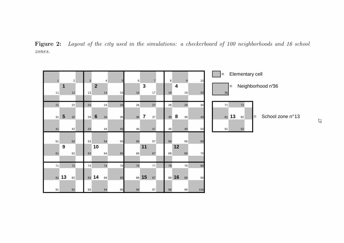
Figure 2: Layout of the city used in the simulations: a checkerboard of 100 neighborhoods and 16 schoolzones.

= Elementary cell1 2 3 4 5 6 7 8 9 10

1 2 3 4 = Neighborhood n°3611 12 13 14 15 16 17 18 19 20 36

21 22 23 24 25 26 27 28 29 30 71 72

31 5 32 33 6 34 35 36 7 37 38 8 39 40 81 13 82 = School zone n° 13

41 42 43 44 45 46 47 48 49 50 91 92

51 52 53 54 55 56 57 58 59 60

9 10 11 1261 62 63 64 65 66 67 68 69 70

71 72 73 74 75 76 77 78 79 80

81 13 82 83 14 84 85 86 15 87 88 16 89 90

91 92 93 94 95 96 97 98 99 100

47

Figure 3: Layout of school zones, neighborhoods, blocks and cells inthe city.

= Elementary cell1 2 3 4 5

1 2 = Neighborhood n° 311 12 13 14 15 3

21 22 23 24 25

3 4 5

31 5 32 33 6 34 35 2 = School zone n° 213 14 15

41 42 43 44 45

block (6,23) formed of 1 elementary cell

block (5,23) formed of 2 elementary cells

block (5,41) formed of 4 elementary cells

48

Figure 4: Simulating school zone reassignments: the new pattern of school attendance boundaries.

= Elementary cell1 2 3 4 5 6 7 8 9 10

3 4 5 6 = Neighborhood n°3611 12 13 14 15 16 17 18 19 20 36

2 721 22 23 24 25 26 27 28 29 30 9

58 59 60

31 32 33 34 35 36 37 38 39 40 = School zone n° 91 8 69 70

41 42 43 44 45 46 47 48 49 50

16 951 52 53 54 55 56 57 58 59 60

61 62 63 64 65 66 67 68 69 70

15 1071 72 73 74 75 76 77 78 79 80

14 13 12 1181 82 83 84 85 86 87 88 89 90

91 92 93 94 95 96 97 98 99 100

49

Figure 5: Distribution of the log of intrinsic neighborhood qualities,the log of family income and the log of pupil ability in the sample of10,000 households used in the simulations.

(a) Log of intrinsic neighborhood quality

(b) Log of family income

(c) Log of pupil ability

50

Figure 6: Simulation example: spatial distribution of neighborhood intrinsic quality.

51

Figure 7: Simulation example: equilibrium spatial distribution ofschool quality and final cell desirability under strict school zoning.

(a) School quality

(b) Final cell desirability

52

Figure 8: Simulation example: relationship between income and celldesirability, intrinsic neighborhood quality and mean ability in the localpublic school under strict school zoning.

(a) Income and global desirability

(b) Income and neighborhood intrinsic quality

(c) Income and mean ability in the local public school

53

Figure 9: Simulating school zone reassignments: comparing initialschool quality to equilibrium school quality.

(a) Initial school quality

(b) Equilibrium school quality

54

Figure 10: Simulating strict school zoning with private schools: equilibrium public and private school quality.

55

Figure 11: Comparing the size of the private sector under strictschool zoning, before and after the reassignments of school zones.

(a) Private schools before reassignments

(b) Private schools after reassignments

56

Figure 12: Comparing public and private school quality under strictschool zoning immediately after the reassignments of school zones andin the final equilibrium.

(a) Initial quality after reassignments

(b) Equilibrium quality after reassignments

57

Figure 13: Simulation example: spatial distribution of the estimated quintiles of intrinsic neighborhood qualityin the city of Paris.

0 1 000 2 000 3 000 4 000 5 000500 Meters

QUINTILES OF INTRINSIC NEIGHBORHOOD QUALITY IN THE CITY OF PARISUnpopulated neighborhoodsQuintile 1Quintile 2Quintile 3Quintile 4Quintile 5

City CenterX

X City "center"

58

Figure 14: Calibrations for Paris. distribution of educational gainsinduced by school zone reassignments and open enrollment, dy decilesof income and ability. Parameter values: λ=0.6. ρ=0.5. β=0.5.s0=0.4.

(a) Average gains from alternative school enrollment policies by decile of income

-1,50

-1,00

-0,50

0,00

0,50

1,00

1,50

1st decile 2nd decile 3rd decile 4th decile 5th decile 6th decile 7th decile 8th decile 9th decile 10th decile

Decile of income

School zonereassignments

Open enrollment

(b) Average gains from alternative school enrollment policies by decile of ability

-1,50

-1,00

-0,50

0,00

0,50

1,00

1,50

1st decile 2nd decile 3rd decile 4th decile 5th decile 6th decile 7th decile 8th decile 9th decile 10th decile

Decile of ability

School zonereassignments

Open enrollment

59

Table 1: Simulation example: residential and educational segregation outcomes from alternative school en-rollment policies.

Parameter values: λ=0.5. ρ=0.5. β=0.5. s0=0.4

Residential Educational Residential Educational Educational Average Average Privatesegregation segregation segregation segregation segregation log ability log ability Enrollment(log income) (log ability) (log income) within public within in public in private (%)

schools: private schools schoolslog abilities schools

Without private schools With private schoolsBenchmarkequilibrium: strict 0.49 0.12 0.35 0.12 0.11 -0.16 0.61 0.20school zoning(s.e.) (0.04) (0.01) (0.05) (0.01) (0.02) (0.02) (0.05) (0.03)

School zonereassignments: 0.18 0.045 0.16initial level(s.e.) (0.05) (0.012) (0.04)

School zonereassignments: 0.32 0.08 0.17 0.11 0.11 -0.21 0.55 0.27final level(SE) (0.06) (0.02) (0.05) (0.01) (0.02) (0.03) (0.03) (0.03)

Openenrollment 0.26 0.98 0.26(s.e.) (0.03) (0.00) (0.03)

Notes: λ: correlation between neighborhood quality and proximity to the city center; ρ: correlation between family income and child ability; β: parental taste

for school quality; s0: seceding threshold to create a private school. Results from 100 simulations performed on random initial spatial distribution of neighborhood

quality, given λ. Standard errors of the estimates are in parentheses.

60

Table 2: Simulation example: distribution of educational gains induced by school zone reassignments and openenrollment in the presence or absence of a private sector.

Parameter values: λ=0.5. ρ=0.5. β=0.5. s0=0.4

Percentage of winners:

Without Private Schools Decile 1th dec. 2nd dec. 3rd dec. 4th dec. 5th dec. 6th dec. 7th dec. 8th dec. 9th dec. 10th dec. TotalSchool zone by income 0.72 0.64 0.61 0.58 0.51 0.48 0.46 0.56 0.45 0.24 0.53reassignments (SRN) by ability 0.62 0.58 0.57 0.56 0.54 0.52 0.50 0.49 0.47 0.42 0.53Open by income 0.32 0.42 0.42 0.46 0.46 0.51 0.53 0.59 0.60 0.67 0.50enrollment (OEN) by ability 0.00 0.00 0.04 0.19 0.37 0.62 0.80 0.95 1.00 1.00 0.50

With Private Schools Decile 1th dec. 2nd dec. 3rd dec. 4th dec. 5th dec. 6th dec. 7th dec. 8th dec. 9th dec. 10th dec. TotalSchool zone by income 0.37 0.51 0.52 0.51 0.47 0.45 0.52 0.55 0.38 0.11 0.44reassignments (SRP) by ability 0.44 0.46 0.46 0.47 0.47 0.45 0.43 0.43 0.41 0.35 0.44Open by income 0.38 0.49 0.47 0.49 0.50 0.52 0.53 0.56 0.52 0.49 0.50enrollment (OEP) by ability 0.00 0.00 0.10 0.25 0.39 0.63 0.75 0.87 0.97 0.99 0.50

Average educational gains:

Without Private Schools Decile 1th dec. 2nd dec. 3rd dec. 4th dec. 5th dec. 6th dec. 7th dec. 8th dec. 9th dec. 10th dec. TotalSchool zone by income 0.13 0.09 0.09 0.06 0.01 -0.02 -0.06 0.00 -0.07 -0.23 0.00reassignments (SRN) by ability 0.07 0.04 0.03 0.03 0.01 0.00 -0.02 -0.03 -0.05 -0.08 0.00Open by income -0.41 -0.15 -0.19 -0.07 -0.09 0.03 0.07 0.21 0.24 0.36 0.00enrollment (OEN) by ability -1.48 -0.93 -0.58 -0.32 -0.13 0.12 0.32 0.59 0.91 1.50 0.00

With Private Schools Decile 1th dec. 2nd dec. 3rd dec. 4th dec. 5th dec. 6th dec. 7th dec. 8th dec. 9th dec. 10th dec. TotalSchool zone by income -0.07 0.02 0.02 0.01 -0.03 -0.04 -0.01 0.02 0.06 0.03 0.00reassignments (SRP) by ability -0.02 -0.01 -0.01 0.00 0.00 0.00 0.00 0.01 0.01 0.02 0.00Open by income -0.24 0.01 -0.08 0.01 0.00 0.07 0.09 0.15 0.03 -0.04 0.00enrollment (OEN) by ability -1.37 -0.85 -0.52 -0.28 -0.10 0.12 0.29 0.54 0.83 1.35 0.00

Notes: λ: correlation between neighborhood quality and proximity to the city center; ρ: correlation between family income and child ability; β: parental taste for school quality;

s0: seceding threshold to create a private school. Results from 100 simulations performed on random initial spatial distribution of neighborhood quality, given λ. Standard errors

of the estimates are in parentheses.

61

Table 3: Calibration for Paris: residential and educational segregation outcomes from alternative schoolenrollment policies.

Parameter values: λ=0.6. ρ=0.5. β=0.5. s0=0.4

Residential Educational Educational Average Average Privatesegregation segregation segregation log ability log ability Enrollment(log income) within public within in public in private (%)

schools: private schools schoolslog abilities schools

Benchmarkequilibrium: strict 0.38 0.12 0.13 -0.23 0.48 0.30school zoning(s.e.) (0.04) (0.01) (0.02) (0.03) (0.04) (0.04)

School zonereassignments: 0.14 0.07initial level(s.e.) (0.04) (0.02)

School zonereassignments: 0.15 0.11 0.14 -0.29 0.42 0.39final level(s.e.) (0.03) (0.00)

Openenrollment 0.31 0.98 0.00(s.e.) (0.03) (0.00)

Notes: λ: correlation between neighborhood quality and proximity to the city center; ρ: correlation between family

income and child ability; β: parental taste for school quality; s0: seceding threshold to create a private school. Results from

100 simulations performed on random initial spatial distribution of neighborhood quality, given λ. Standard errors of the

estimates are in parentheses.

62

Table 4: Calibration for Paris: distribution of educational gains induced by school zone reassignments andopen enrollment.

Parameter values: λ=0.6. ρ=0.5. β=0.5. s0=0.4

Percentage of winners:

Decile 1th dec. 2nd dec. 3rd dec. 4th dec. 5th dec. 6th dec. 7th dec. 8th dec. 9th dec. 10th dec. TotalSchool zone by income 0.34 0.50 0.51 0.49 0.45 0.45 0.50 0.51 0.14 0.04 0.39reassignments by ability 0.42 0.44 0.43 0.44 0.43 0.40 0.38 0.37 0.34 0.28 0.39Open by income 0.42 0.51 0.49 0.50 0.50 0.51 0.51 0.55 0.49 0.48 0.50enrollment by ability 0.00 0.01 0.12 0.26 0.40 0.61 0.74 0.86 0.96 0.99 0.50

Average gains:

Decile 1th dec. 2nd dec. 3rd dec. 4th dec. 5th dec. 6th dec. 7th dec. 8th dec. 9th dec. 10th dec. TotalSchool zone by income -0.07 0.01 0.01 0.00 -0.02 -0.02 0.01 0.04 0.02 0.01 0.00reassignments by ability -0.02 -0.01 0.00 0.00 0.00 0.00 0.00 0.01 0.01 0.01 0.00Open by income -0.14 0.05 -0.05 0.03 0.01 0.05 0.03 0.11 -0.03 -0.06 0.00enrollment by ability -1.33 -0.83 -0.51 -0.28 -0.10 0.12 0.28 0.53 0.80 1.32 0.00

Notes: λ: correlation between neighborhood quality and proximity to the city center; ρ: correlation between family income and child ability; β: parental taste for

school quality; s0: seceding threshold to create a private school. Results from 100 simulations performed on random initial spatial distribution of neighborhood quality,

given λ. Standard errors of the estimates are in parentheses.

63