a spatially explicit methodology to quantify soil nutrient ...late soil nutrient balances in a...

ORIGINAL PAPER

A spatially explicit methodology to quantify soil nutrientbalances and their uncertainties at the national level

J. P. Lesschen Æ J. J. Stoorvogel ÆE. M. A. Smaling Æ G. B. M. Heuvelink ÆA. Veldkamp

Received: 4 May 2006 / Accepted: 8 December 2006 / Published online: 23 January 2007� Springer Science+Business Media B.V. 2007

Abstract A soil nutrient balance is a commonly

used indicator to assess changes in soil fertility. In

this paper, an earlier developed methodology by

Stoorvogel and Smaling to assess the soil nutrient

balance is given a major overhaul, based on

growing insights and advances in data availability

and modelling. The soil nutrient balance is

treated as the net balance of five inflows (mineral

fertilizer, organic inputs, atmospheric deposition,

nitrogen fixation and sedimentation) and five

outflows (crop products, crop residues, leaching,

gaseous losses and erosion). This study aims to

improve the existing methodology by making it

spatially explicit, improving various transfer func-

tions, and by modelling explicitly the uncertain-

ties in the estimations. Spatially explicit

modelling has become possible through a novel

methodology to create a simulated land use map

on the basis of the principles of traditional

qualitative land evaluation. New literature data

on the various inputs and outputs allowed

improvement of the estimations of deposition,

sedimentation, leaching, and erosion. Moreover,

the uncertainty of the calculated soil nutrient

balances was assessed. To illustrate the

improved methodology, we applied it to Burkina

Faso and revealed that nutrient depletion is

occurring throughout the country at rates

of �20� 15 kg N ha�1, �3:7� 2:9 kg P ha�1 and

�15� 12 kg K ha�1. The resulting spatial soil

nutrient balances at the national level can consti-

tute the basis for targeting soil fertility policies at

lower levels.

Keywords Land use � Soil fertility � Soil nutrient

balance � Spatially explicit � Uncertainty analysis

Introduction

A soil nutrient balance is a commonly used

indicator to assess changes in soil fertility (e.g.,

Bindraban et al. 2000; Roy et al. 2003). Stoorvo-

gel and Smaling (1990) introduced a soil nutrient

balance as a net balance of five inflows and five

J. P. Lesschen (&)Institute for Biodiversity and Ecosystem Dynamics,University of Amsterdam, Nieuwe Achtergracht 166,1018WV Amsterdam, The Netherlandse-mail: [email protected]

J. J. Stoorvogel � G. B. M. Heuvelink � A. VeldkampLandscape Centre, Wageningen University, P.O. Box37, 6700AA Wageningen, The Netherlands

E. M. A. SmalingInternational Institute for Geo-Information Scienceand Earth Observation, P.O. Box 6, 7500AAEnschede, The Netherlands

E. M. A. SmalingPlant Production Systems Group, WageningenUniversity, P.O. Box 430, 6700AK Wageningen,The Netherlands

123

Nutr Cycl Agroecosyst (2007) 78:111–131

DOI 10.1007/s10705-006-9078-y

outflows, which indicates whether an agricultural

system is a net winner or loser in terms of soil

fertility. They constructed N, P and K balances

for 37 sub-Saharan countries, which revealed that

soil fertility is generally following a downward

trend on the African continent (Stoorvogel and

Smaling 1990; Stoorvogel et al. 1993). Although

the methodology has been widely used, it was also

criticized for lack of validation, the use of simple

transfer functions, and not taking into account

spatial and temporal variability and unknown

uncertainties (Scoones and Toulmin 1998; Har-

temink 2003; Faerge and Magid 2004). Practical

alternatives were, however, not suggested, and

the ‘old’ methodology continued to be applied

until today. In the meantime many more data

have become available to develop better vali-

dated regression models or to have them replaced

altogether by more advanced simulation models.

Furthermore, new geographic data sets and

remote sensing images make it possible to calcu-

late soil nutrient balances in a spatially explicit

way. As a result regional differences due to soil

and climate variability can be taken into account

and national soil fertility policies can be better

targeted towards the lower levels, e.g., district or

cooperation region (FAO 2004).

The objective of this study was to revisit the

methodology developed by Stoorvogel and Smal-

ing (1990). No changes were made to the overall

goal of the methodology to assess soil nutrient

balances for agricultural land in any African

country using publicly available data. Where the

basic conceptual framework did not change, we

focused the improvements on:

• Developing techniques to make the methodol-

ogy spatially explicit. The original study used

the so-called ‘‘land-water classes’’ (FAO 1978;

Alexandratos 1988) as the basic calculation

units. A better assessment of the soil nutrient

balances is only possible if land use maps are

available. A new methodology to develop these

land use maps need to be developed. Only then,

land use maps can be overlain by other spatially

explicit data (e.g., soil and climate).

• Re-estimating the original regression models

for the various nutrient flows or, if possible,

replace them by simple simulation models.

New data sets and models have become

available that allow more accurate assessment

of some of the processes.

• Assessing the uncertainties of soil nutrient

balance estimates. Even at the farm level with

detailed data, assessing the soil nutrient bal-

ance is found to be difficult. So, how accurate

are the assessments for an entire country? It is

clear that a proper evaluation of the accuracy

of these nutrient balances is important.

The first part of our paper describes the

changes that we propose for the assessment of

the soil nutrient balances. Next, we present the

results for an application of the methodology for

Burkina Faso. Finally, the soil nutrient balance

methodology and its uncertainty analysis are

discussed.

The new methodology

The soil nutrient balance methodology includes a

large number of different steps including the

methodology to create a land use map and the

estimation of each of the individual nutrient

flows. This is followed by the actual calculation

of the soil nutrient balance and an evaluation of

the accuracy of the estimation. The various flows

are summarized in Table 1 with the improve-

ments applied in this study. Each flow is defined

in this section.

Land use map

Nutrient balances reflect particular land use

systems, including soil and climatic conditions.

As a result the calculation can only take place on

a site-specific basis in which soil, climate and

crops are superimposed. Various authors devel-

oped approaches to calculate spatially explicit soil

nutrient balances. Folmer et al. (1998), for exam-

ple, made an assessment of soil fertility depletion

in Mozambique using land units and land use

types and calculated the soil nutrient balance

following Stoorvogel and Smaling (1990). The

approach was spatially explicit, but still based on

classes instead of all soil and topographical

characteristics and generalized land use systems

112 Nutr Cycl Agroecosyst (2007) 78:111–131

123

instead of individual crops. Furthermore, the

compilation of the land use system map was not

straightforward and remained country-specific.

De Koning et al. (1997) and Priess et al. (2001)

calculated spatially explicit soil nutrient balances

for Ecuador, following the methodology of Sto-

orvogel and Smaling (1990) for grid cells of 5 arc

minutes. A land use map was constructed indi-

rectly by relating sample sites of the national

agricultural statistics census to grid cells. Such an

approach is suitable when a sound, geo-refer-

enced system of agricultural statistics is available.

However, for African countries such a database is

normally not available.

The estimation of nutrient flows and balances

starts with the definition of the various land use

systems. Therefore we considered a land use map

to be the appropriate basis for the methodology.

However, land cover data, as derived from

satellite images, do not describe crop distribution

at the national level with sufficient detail, i.e.,

only agricultural areas or crop groups can be

distinguished. On the other hand, national statis-

tics, such as provided by the FAOSTAT database,

are not spatially explicit and can therefore not be

linked directly to climate and soil data. To solve

this problem we developed a new methodology,

which generates land use maps for sub-Saharan

African countries on the basis of available data-

sets. The proposed methodology is based on the

principles of qualitative land evaluation, where

land qualities are matched with land use require-

ments to assess the suitability of land for a given

use (FAO 1976). The methodology is based on

three key steps:

1. Identify land units with similar topography,

climate and soil conditions.

2. Match properties of the land units with crop

requirements.

3. Disaggregate harvested areas from FAO-

STAT over the land units.

Land use map step 1

In a first step, land units are identified, as defined

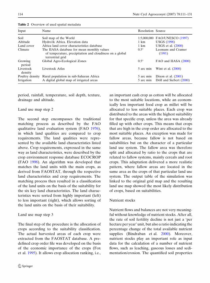
by topography, soil and climate. Metadata of the

used datasets are described in Table 2. Quantita-

tive data for the FAO soil map of the world

(FAO/UNESCO 1997) were derived from the

World Inventory of Soil Emission potential

(WISE) database (Batjes 2002). This database

consists of a set of homogenized worldwide data

of 4382 geo-referenced soil profiles, classified

according to the FAO-UNESCO original legend

(1974) and the revised legend of 1988. Finally, the

agricultural areas were identified from the land

cover map using a reclassified version of the

‘seasonal land cover region’ legend (USGS et al.

2000). All maps were overlain into a single 1-km

grid. The databases were linked and a table with

the following land characteristics was created for

each grid cell: land cover, length of growing

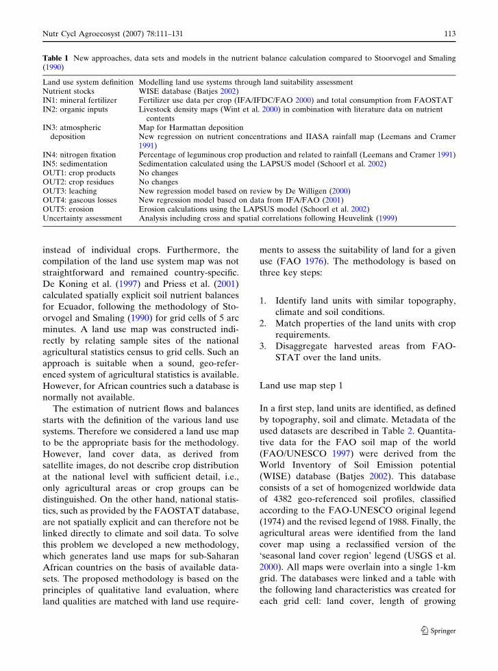
Table 1 New approaches, data sets and models in the nutrient balance calculation compared to Stoorvogel and Smaling(1990)

Land use system definition Modelling land use systems through land suitability assessmentNutrient stocks WISE database (Batjes 2002)IN1: mineral fertilizer Fertilizer use data per crop (IFA/IFDC/FAO 2000) and total consumption from FAOSTATIN2: organic inputs Livestock density maps (Wint et al. 2000) in combination with literature data on nutrient

contentsIN3: atmospheric

depositionMap for Harmattan depositionNew regression on nutrient concentrations and IIASA rainfall map (Leemans and Cramer1991)

IN4: nitrogen fixation Percentage of leguminous crop production and related to rainfall (Leemans and Cramer 1991)IN5: sedimentation Sedimentation calculated using the LAPSUS model (Schoorl et al. 2002)OUT1: crop products No changesOUT2: crop residues No changesOUT3: leaching New regression model based on review by De Willigen (2000)OUT4: gaseous losses New regression model based on data from IFA/FAO (2001)OUT5: erosion Erosion calculations using the LAPSUS model (Schoorl et al. 2002)Uncertainty assessment Analysis including cross and spatial correlations following Heuvelink (1999)

Nutr Cycl Agroecosyst (2007) 78:111–131 113

123

period, rainfall, temperature, soil depth, texture,

drainage and altitude.

Land use map step 2

The second step encompasses the traditional

matching process as described by the FAO

qualitative land evaluation system (FAO 1976),

in which land qualities are compared to crop

requirements. The land qualities were repre-

sented by the available land characteristics listed

above. Crop requirements, expressed in the same

way as land characteristics, were described by the

crop environment response database ECOCROP

(FAO 1998). An algorithm was developed that

matches the land units with the main crops, as

derived from FAOSTAT, through the respective

land characteristics and crop requirements. The

matching process then resulted in a classification

of the land units on the basis of the suitability for

the six key land characteristics. The land charac-

teristics were sorted from highly important (left)

to less important (right), which allows sorting of

the land units on the basis of their suitability.

Land use map step 3

The final step of the procedure is the allocation of

crops according to the suitability classification.

The actual harvested areas of each crop were

extracted from the FAOSTAT database. A pre-

defined crop order file was developed on the basis

of the economic importance of the crops (Fox

et al. 1995). It allows crop allocation ranking, i.e.,

an important cash crop as cotton will be allocated

to the most suitable locations, while an econom-

ically less important food crop as millet will be

allocated to less suitable places. Each crop was

distributed to the areas with the highest suitability

for that specific crop, unless the area was already

filled up with other crops. This means that crops

that are high in the crop order are allocated to the

most suitable places. An exception was made for

fallow areas, because fallow is not based on

suitabilities but on the character of a particular

land use system. The fallow area was therefore

split and allocated by ratio to the crops that are

related to fallow systems, mainly cereals and root

crops. This adaptation delivered a more realistic

pattern, where fallow areas are located in the

same area as the crops of that particular land use

system. The output table of the simulation was

linked to the original grid map and the resulting

land use map showed the most likely distribution

of crops, based on suitabilities.

Nutrient stocks

Nutrient flows and balances are not very meaning-

ful without knowledge of nutrient stocks. After all,

the rate of soil fertility decline is not just a ‘per

hectare per year’ unit, but also a ratio indicating the

percentage change of the total available nutrient

supplies (Bindraban et al. 2000). Moreover,

nutrient stocks play an important role as input

data for the calculation of a number of nutrient

flows, such as leaching, gaseous losses and sedi-

mentation/erosion. The quantified soil properties

Table 2 Overview of used spatial metadata

Input Name Resolution Source

Soil Soil map of the World 1:5,000,000 FAO/UNESCO (1997)Altitude Hydro1k Africa. Elevation data 1 km USGS (1998)Land cover Africa land cover characteristics database 1 km USGS et al. (2000)Climate The IIASA database for mean monthly values

of temperature, precipitation and cloudiness on a globalterrestrial grid

0.5� Leemans and Cramer(1991)

Growingperiod

Global Agro-Ecological Zones 0.5� FAO and IIASA (2000)

Livestockdensity

Livestock Atlas 5 arc min Wint et al. (2000)

Poultry density Rural population in sub-Saharan Africa 5 arc min Dixon et al. (2001)Irrigation A digital global map of irrigated areas 5 arc min Doll and Siebert (2000)


123

were derived from the WISE database (Batjes

2002). The soil profiles from Africa were extracted

from this database, yielding 1799 different soil

profiles. The following soil properties were calcu-

lated for each soil unit: clay, pH, organic carbon,

total N, exchangeable K, CEC, available P and bulk

density. Soil depth and erodibility, necessary for the

erosion–sedimentation model, are not included in

the WISE database and therefore each soil unit was

classified to a soil depth and a soil erodibility class

based on general descriptions of soil groups and units

(FAO 2001). The nutrient stocks were calculated for

the first 30 cm of the soil, which was straightforward

for N, but more complicated for P and K, since the

WISE database has ‘available’ rather than ‘total’

values of these nutrients. Therefore, available P was

converted to total P according to the classes of

Langdon (1991), and for K only exchangeable K was

used, since a very large part of total K in the soil is not

available as nutrient.

Soil nutrient balance

To calculate the soil nutrient balances the simu-

lated land use map was combined with other

spatial data needed for calculations, which lead to

a single database with all spatial data for each 1-

km grid cell. Calculation of the nutrient flows and

balance, as explained in detail below, was done in

a database program. The results were exported to

a GIS to create spatially explicit maps and to

aggregate the results. We chose a resolution of 20-

km for the aggregation, which still provided

sufficient detail to represent the variation within

a country, but also justified the use of input data

at less detailed resolution, i.e., soil and climate

data. Besides, aggregation leads to a reduction of

the uncertainty of the soil nutrient balance

results, because of averaging effects.

IN1: mineral fertilizer

Mineral fertilizer input was calculated per crop as

a fraction of the total national fertilizer consump-

tion, obtained from FAOSTAT. The fractions

were based on data of the ‘fertilizer use per crop’

studies of IFA/IFDC/FAO (2000). However,

these data are not available for each country, in

which case the fractions were estimated with data

from surrounding countries with similar agro-

ecological zones, e.g., for Burkina Faso data from

Mali and Senegal was used.

IN2: organic inputs

Manure is the main organic input for most

African countries and is related to the number

of livestock. Livestock density maps for the major

livestock classes, i.e., cattle and small ruminants

(sheep and goats), provided the spatial distribu-

tion of livestock over the country. These maps

were based on climate, geography, population

density and statistical data (Wint et al. 2000).

Since no poultry density map was available, we

created one based on the rural population map of

sub-Saharan Africa (Dixon et al. 2001), for which

we assumed a linear relationship between rural

population density and the abundance of poultry.

The total amount of nutrients from manure

was calculated by multiplying the livestock den-

sities by the excretion per animal per year and the

nutrient content of the manure for each livestock

class. The nutrient content and excretion factors

(Table 3) were based on various literature

sources for African conditions (Baijukya et al.

1998; Budelman and Defoer 2000; Lekasi et al.

2001; Smaling et al. 1999; Williams et al. 1995).

Based on the livestock maps the total amount

of nutrients produced could be calculated. How-

ever, losses and distribution still had to be

determined. According to Fernandez-Riviera

et al. (1995) and Schlecht et al. (1995), 43% of

the manure is excreted at night, when animals are

in their stable/corral/boma. This amount, losses

excluded, can be relocated to specific crops. The

remaining 57% of the manure, losses excluded,

remains on the field. Livestock from grid cells that

were not classified as cropland, e.g., pasture land,

had to be included, because part of the nutrients

Table 3 Nutrient content of manure (fresh weight) andexcretion

N (%) P (%) K (%) Excretiona

Cattle manure 0.76 0.15 0.67 6.2Sheep/goat manure 0.79 0.20 0.50 7.2Poultry manure 1.08 0.39 0.35 7.8

a Excretion in kg fresh matter per kg body weight per year


123

from pastures is transferred to stables and after-

wards to other crops. The livestock density maps

were therefore aggregated to a 20-km grid repre-

senting the livestock density of that region. This

value was multiplied by an aggregation factor and

a crop factor. The estimated aggregation factor

was country dependent and related to the human

population density, i.e., more manure relocation

occurs in countries with a higher population

density (e.g., Ethiopia). An estimated crop factor

determined if a specific crop received manure (1),

double quantity of manure (2) or no manure (0).

During grazing, manure losses occur along

roadsides and other places where no crops are

growing. These losses were estimated at 15% for

each country. Losses during storage were esti-

mated to be larger, because farmers use manure for

other purposes as well, e.g., fuel or construction

material. Losses also occur because of storage

itself, manifested through leaching, denitrification

and volatilization. Since this loss factor depends on

the type of management, it was estimated for each

country, based on population density, livestock

system and the relative importance of manure as a

fertilizer, e.g., ‘zero grazing’ versus ‘free range’

systems. Losses due to leaching, denitrification and

volatilization for the calculated manure applica-

tion were accounted for in OUT3 and OUT4. The

final calculation of organic inputs per grid cell for

each livestock class (cattle, small ruminants and

poultry) can be written as:

IN2 ¼ðlivestock density�excretion

�nutrient content� losses (grazing)Þþ (aggregated livestock density

�aggregation factor� crop factor

�excretion�nutrient content

� losses (storage))

ð1Þ

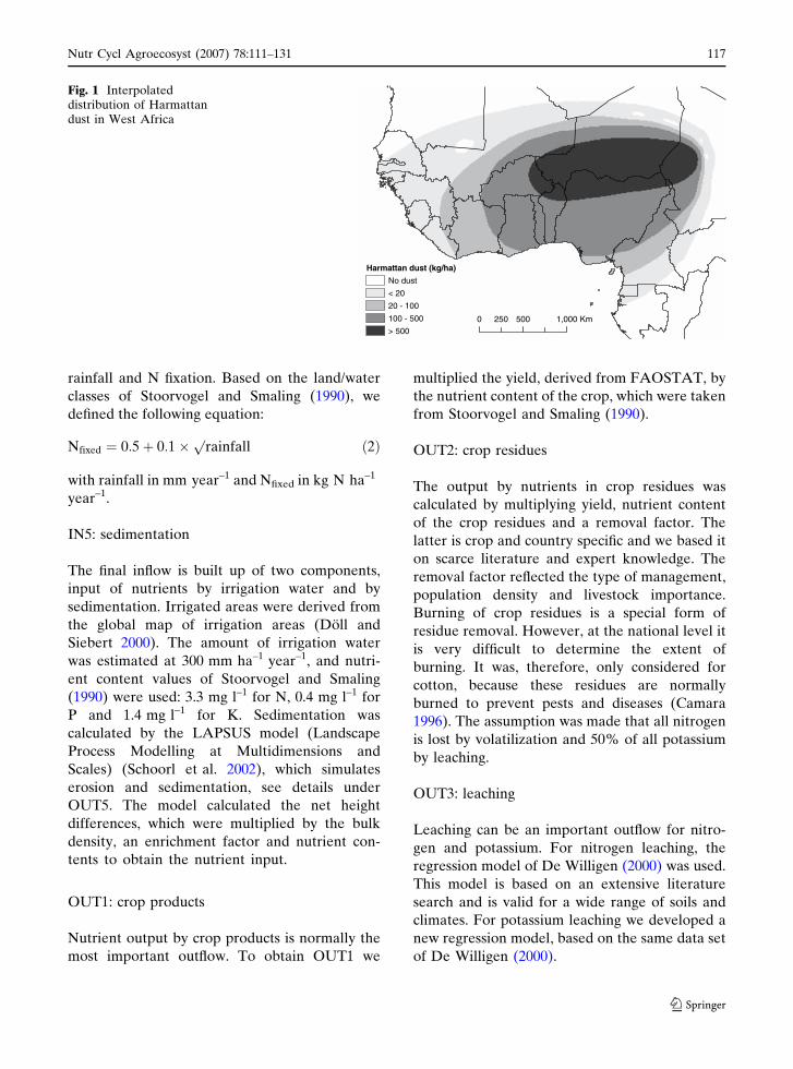
IN3: atmospheric deposition

Atmospheric deposition occurs in two forms,

wet deposition related to rainfall and dry

deposition related to Harmattan dust. Wet

deposition also includes nitrogen fixation

through lightning, because formed NOx dis-

solves in water and precipitates during rainfall.

This is an important source of nitrogen, espe-

cially for the wet tropics, where many lightning

storms occur (Bond et al. 2002). The amount of

precipitation was derived from the IIASA

rainfall map (Leemans and Cramer 1991).

Nutrient concentrations are based on a regres-

sion of relevant measurements in Africa

(Langenberg et al. 2002; Stoorvogel et al.

1997b; Bruijnzeel 1990; Baudet et al. 1989; Pieri

1985; Jones and Bromfield 1970; Richard 1963;

Meyer and Pampfer 1959) with an average

value of 4.9±2.5 g N ha–1 mm–1, 0.6±0.5 g P

ha–1 mm–1 and 2.6±1.1 g K ha–1 mm–1. For Har-

mattan dust we created a map (Fig. 1), based

on interpolation of the dust measurements and

wind stream patterns with an average nutrient

content of 3.8±0.6 g N kg–1 dust, 0.8±0.4 g P

kg–1 dust and 19±12 g K kg–1 dust (Stoorvogel

et al. 1997a; Drees et al. 1993; Moberg et al.

1991; Tiessen et al. 1991; Pye 1987; McTainsh

and Walker 1982; McTainsh 1980; Kalu 1979).

IN4: nitrogen fixation

Biological nitrogen fixation is an important

source of nitrogen for leguminous crops through

symbiosis, but other crops can also profit

indirectly through non-symbiotic N fixation

and N fixing trees. Values for symbiotic N

fixation were obtained from literature and

expressed as percentages of total N uptake:

groundnut 65%, soybean 67%, pulses 55% and

sugarcane 17% (Giller 2001; Danso 1992; Giller

and Wilson 1991; Hartemink 2003).

Non-symbiotic N fixation by cyanobacteria is an

important process in soils under wetland rice. We

estimated the contribution at 15 kg N ha–1 year–1,

which is lower than most experiments revealed,

but according to Giller (2001) the effect of cyano-

bacteria is overestimated and does not occur in all

fields. N fixation by cyanobacteria only occurs

under wetland rice, however, the FAOSTAT data

do not differentiate between wetland and upland

rice. The value was therefore multiplied by the

cropping index of wetland rice according to IPCC

(1997). As last we accounted for small contribu-

tions from non-symbiotic N fixation and N fixing

trees assuming a positive relationship between


123

rainfall and N fixation. Based on the land/water

classes of Stoorvogel and Smaling (1990), we

defined the following equation:

Nfixed ¼ 0:5þ 0:1�prainfall ð2Þ

with rainfall in mm year–1 and Nfixed in kg N ha–1

year–1.

IN5: sedimentation

The final inflow is built up of two components,

input of nutrients by irrigation water and by

sedimentation. Irrigated areas were derived from

the global map of irrigation areas (Doll and

Siebert 2000). The amount of irrigation water

was estimated at 300 mm ha–1 year–1, and nutri-

ent content values of Stoorvogel and Smaling

(1990) were used: 3.3 mg l–1 for N, 0.4 mg l–1 for

P and 1.4 mg l–1 for K. Sedimentation was

calculated by the LAPSUS model (Landscape

Process Modelling at Multidimensions and

Scales) (Schoorl et al. 2002), which simulates

erosion and sedimentation, see details under

OUT5. The model calculated the net height

differences, which were multiplied by the bulk

density, an enrichment factor and nutrient con-

tents to obtain the nutrient input.

OUT1: crop products

Nutrient output by crop products is normally the

most important outflow. To obtain OUT1 we

multiplied the yield, derived from FAOSTAT, by

the nutrient content of the crop, which were taken

from Stoorvogel and Smaling (1990).

OUT2: crop residues

The output by nutrients in crop residues was

calculated by multiplying yield, nutrient content

of the crop residues and a removal factor. The

latter is crop and country specific and we based it

on scarce literature and expert knowledge. The

removal factor reflected the type of management,

population density and livestock importance.

Burning of crop residues is a special form of

residue removal. However, at the national level it

is very difficult to determine the extent of

burning. It was, therefore, only considered for

cotton, because these residues are normally

burned to prevent pests and diseases (Camara

1996). The assumption was made that all nitrogen

is lost by volatilization and 50% of all potassium

by leaching.

OUT3: leaching

Leaching can be an important outflow for nitro-

gen and potassium. For nitrogen leaching, the

regression model of De Willigen (2000) was used.

This model is based on an extensive literature

search and is valid for a wide range of soils and

climates. For potassium leaching we developed a

new regression model, based on the same data set

of De Willigen (2000).

Harmattan dust (kg/ha)

No dust

< 20

20 - 100

100 - 500

> 5000 500 1,000250 Km

Fig. 1 Interpolateddistribution of Harmattandust in West Africa


123

OUT3Nðkg N ha�1year�1Þ¼ ð0:0463þ 0:0037� ðP=ðC� LÞÞÞ� ðFN þD�NOM�UÞ

ð3Þ

OUT3Kðkg N ha�1year�1Þ¼ �6:87þ 0:0117

� Pþ 0:173� FK � 0:265� CEC

ð4Þ

where

P = precipitation (mm year–1)

C = clay (%)

L = layer thickness (m) = rooting depth, derived

from Allen et al. (1998)

FN = mineral and organic fertilizer nitrogen

(kg N ha–1 year–1)

D = decomposition rate of organic matter (1.6%

year–1)

NOM = amount of nitrogen in soil organic matter

(kg N ha–1)

U = uptake by crop (kg N ha1 year–1)

FK = mineral and organic fertilizer potassium

(kg K ha–1 year–1)

CEC = cation exchange capacity (cmol kg–1)

The N leaching regression model was based

on 43 experiments and accounted for 67% of

the variance (De Willigen 2000). The equation

was slightly adapted for perennial crops by

multiplying the amount of available nitrogen

from soil organic matter with 0.5. This pre-

vented overestimation of N leaching, because

perennials take up nitrogen throughout the

year, contrary to annual crops. Moreover, most

of the leaching experiments were conducted

under annual crops. The K leaching regression

model was based on 33 representative experi-

ments and accounted for 45% of the variance.

OUT4: gaseous losses

Denitrification and volatilization are the main

processes for gaseous nitrogen emissions. Deni-

trification takes place under anaerobic condi-

tions, although a soil does not have to be

entirely saturated for denitrification to take

place. A moist soil already loses nitrate through

microbial processes in wet films and pockets.

We expected nitrogen losses through denitrifica-

tion to be highest in wet climates, on highly

fertilized and clayey soils. Ammonia volatiliza-

tion is linked to the amount of mineral and

organic fertilizer and plays a role in alkaline

environments (Bouwman 1998). However, such

soils are not very common in sub-Sahara Africa.

Volatilization was therefore not treated sepa-

rately, but together with denitrification. We

developed a regression model to estimate gas-

eous losses for N2O, NOx and NH3, based on

literature data for tropical environments, derived

from a larger data set (IFA/FAO 2001). The

regressions were combined into the following

equation, which had an R2 of 0.70.

OUT4 ðkg N ha�1year�1Þ¼ 0:025þ 0:000855

� Pþ 0:130� Fþ 0:117�O

ð5Þ

where

P = precipitation (mm year–1)

F = mineral and organic fertilizer nitrogen (kg N

ha–1 year–1)

O = soil organic carbon content (%)

OUT5: erosion

To estimate erosion we used the LAPSUS

model (Schoorl et al. 2002). The model simu-

lates the amount of water erosion and sedimen-

tation at the landscape scale and has been

calibrated with 137Cs for a study area in

Southern Spain (Schoorl et al. 2004). The

advantages of process-based modelling of soil

redistribution are the generation of quantitative

data, consideration of erosion at landscape scale

and inclusion of sedimentation. We preferred

modelling above literature estimates, which are

mainly based on plot experiments that are

generally not representative for the national

level (Schulze 2000).

The modelling approach is based on the

principle of the potential energy content of

flowing water over a landscape surface as the

driving force for sediment transport (Kirkby

1986) and the use of the continuity equation


123

for sediment movement (Foster and Meyer

1975). The model evaluates the rates of sediment

transport by calculating the transport capacity of

water flowing downslope from one grid cell to

another as a function of discharge and slope

gradient. A surplus of capacity is compensated

by detachment of sediment, depending on the

erodibility of the surface, which provokes ero-

sion. When the rate of sediment in transport

exceeds the local capacity, the surplus is depos-

ited, causing sedimentation. Routing of overland

flow and resulting model calculations were done

with a multiple flow algorithm to allow for a

better representation of divergent properties of a

convex topography.

Main input data of the LAPSUS model are

the topographical potentials derived from a

digital elevation model (USGS 1998) and rainfall

surplus, derived from the rainfall map (Leemans

and Cramer 1991). Other input data are soil

depth and erodibility, which were based on the

soil map (FAO/UNESCO 1997), and a land

cover map (USGS et al. 2000). With these inputs

the model simulated runoff and erosion–sedi-

mentation for one year at a 1-km resolution. The

loss or gain of nutrients was calculated by

multiplying the erosion or sedimentation by the

soil nutrient contents and an enrichment factor.

This factor was introduced, because finer and

more fertile soil particles are dislodged first

during erosion. Enrichment factors were set at

2.3 for N, 2.8 for P and 3.2 for K, based on

Stocking (1984, 1986), Cogle et al. (2002) and

Khisa et al. (2002).

Fallow

The FAO statistics give no information about the

area under fallow. However, it was possible to

calculate the fallow area indirectly by subtracting

the total sum of harvested areas from the total

arable land area. However, this calculation only

included temporarily uncropped arable land, but

not bush fallow. The latter is not recognized as

arable land on satellite images and not included in

the FAO statistics. The procedure to calculate the

soil nutrient balance for fallow was slightly

different, because it is not like a crop for which

production data are available. Mineral fertilizer

(IN1) and crop product (OUT1) are not relevant

for fallow. IN2 and OUT2 are related to each

other by grazing and defecating livestock, how-

ever, it was unknown whether IN2 should be

greater or smaller than OUT2. Not all manure is

left on the field (only about 57%), but on the

other hand a lot of animal feedstuff is obtained

from sources other than crop residues, e.g.,

roadside grazing. Hence, for fallow land we

assumed the amount of nutrient input by manure

(IN2) to be equal to the amount lost by grazing

(OUT2). All other nutrient flows were treated

equally as for other crops.

Uncertainty assessment

The results of the soil nutrient balance are only

meaningful when they have sufficient accuracy. It

is risky to draw conclusions and base decisions on

results that are untrustworthy and that may

deviate strongly from reality. The soil nutrient

balance calculations are based on several assump-

tions and simplifications, and hence the risk of

highly uncertain results is present. To analyse the

accuracy of these results, it was necessary to track

down how uncertainties in the input variables

propagate to the soil nutrient balance results. This

was not an easy task, because there are many

inputs and the uncertainties associated with these

variables are largely unknown. The uncertainty

analysis also had to take cross and spatial corre-

lations between the various uncertainties and the

scale-dependency of uncertainties into account

(Heuvelink 1999). In spite of these difficulties, we

estimated the uncertainties of the variables and

calculated how these propagate to the final

results.

The soil nutrient balance and flow calculation

involved sums and products of variables. In case of

summation, the calculation may be formulated as:

Y ¼Xn

i¼1

aiXi ð6Þ

where Y is the resulting soil nutrient balance and

Xi is the nutrient in- and outputs. The multipli-

cation factors ai are introduced to allow both

for addition (ai = 1) and subtraction (ai = –1).


123

The expected value (lY) and variance (rY2 ) of Y

are given by:

lY ¼Xn

i¼1

aili ð7Þ

r2Y ¼

Xn

i¼1

a2i r

2i þ 2

Xn�1

i¼1

Xn

j¼iþ1

aiajqijrirj ð8Þ

where li and ri are the mean and standard

deviation of Xi, respectively, and where qij is

the correlation coefficient between the

uncertainties in Xi and Xj. Next, we consider

the case in which the nutrient flow is defined as

the product of variables:

Y ¼ X1 �X2 � � � � �Xn ¼Yn

i¼1

Xi ð9Þ

Calculation of the mean and variance of Y is

more complicated in this case. However, by

assuming that the Xi are uncorrelated and

ignoring higher order terms in the Taylor series

expansion of the product function, we obtain

(Heuvelink 1998):

lY ffiYn

i¼1

li ð10Þ

r2Y ffi

Xn

i¼1

r2i

l2i

Yn

j¼1

l2j

!

¼Xn

i¼1

r2i � l2

1 � l22 � � � � � l2

i�1 � l2iþ1 � l2

iþ2 � � � � � l2n

ð11Þ

The uncertainties in the variables (Table 4)

were either estimated, e.g., for the fertilizer use

per crop parameters, or calculated, e.g., for the

nutrient content of manure. The relative uncer-

tainties for each nutrient flow could then be

calculated according to Eqs. (8) and (11), where-

by all uncertainties of the variables were consid-

ered uncorrelated.

The uncertainty of the total soil nutrient

balance can be calculated when the relative

uncertainties of all nutrient flows are known.

However, not all nutrient flows are independent,

some flows are correlated to others, e.g., the

gaseous nitrogen losses are correlated to the

mineral fertilizer and organic inputs. The covari-

ance of the correlated flows should therefore be

included in the uncertainty analyses (Oenema

and Heinen 1999). With Eq. (8) the variance of

the soil nutrient balance was calculated, including

the covariance for the correlated nutrient flows

(Table 5). The correlation coefficients (qij) were

calculated with SPSS (Pearsons correlation),

based on the calculated nutrient flows for each

grid cell. The correlation coefficient was set to 0

for correlations between nutrient flows other than

those given in Table 5.

Spatial aggregation

For each grid cell, the variance could now be

calculated at the 1-km resolution. However, these

results were aggregated to a 20-km grid, which

influenced the variance of the soil nutrient

balance because part of the variation and hence

uncertainty was cancelled. Spatial aggregation

can be formulated as:

Yagg ¼1

n

Xn

i¼1

Yi ð12Þ

where Yagg is the aggregated soil nutrient balance,

Yi is the soil nutrient balance for the ith grid cell

and n the number of aggregated grid cells (in our

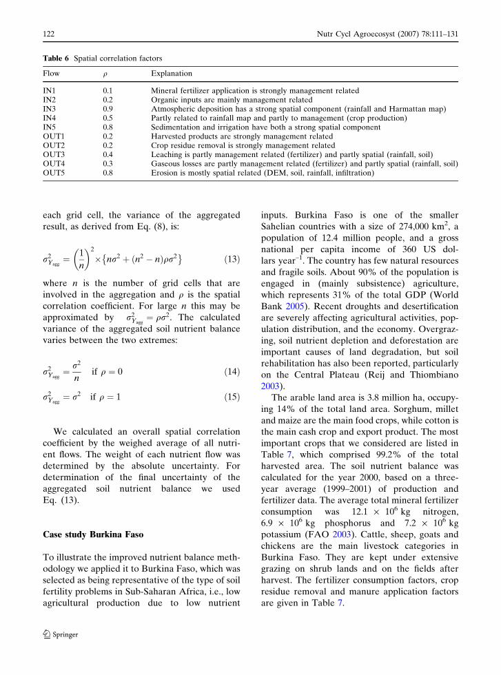
case n = 400). Spatial correlation occurs because

part of the input data is spatially dependent, e.g.,

soil and rainfall data. We estimated the spatial

correlation coefficient for each nutrient flow

(Table 6), which ranged between 0 and 1. It

indicates how the value of each nutrient flow in

influenced by nearby observations, e.g., mineral

fertilizer input is hardly spatially correlated,

because one farmer can apply much fertilizer,

while his neighbour might apply nothing.

Atmospheric deposition, on the other hand, is

highly spatially correlated, because variation in

rainfall and dust deposition is not much at short

distances. The degree of spatial correlation affects

the variance of the aggregated results. In general,

assuming that the variance of Yi (r2) is equal for


123

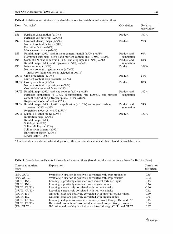
Table 4 Relative uncertainties as standard deviations for variables and nutrient flows

Flow Variablesa Calculation Relativeuncertainty

IN1 Fertilizer consumption (±10%) Product 100%Fertilizer use per crop (±100%)

IN2 Livestock density maps (±20%) Product 91%Nutrient content factor (± 50%)Excretion factor (±20%)Management factor (±70%)

IN3 Rainfall map (±20%) and nutrient content rainfall (±50%) �54%Harmattan dust map (±75%) and nutrient content dust (± 50%) �90%

Product andsummation

60%

IN4 Symbiotic N-fixation factors (±30%) and crop uptake (±50%) �58%Rainfall map (±20%) and regression (±50%) �54%


60%

IN5 Irrigation map (±30%) Product 104%Nutrient content irrigation water (±100%)

(Error for sedimentation is included in OUT5)OUT1 Crop production (±50%) Product 58%

Nutrient content crop products (±30%)OUT2 Crop production (±50%) Product 87%

Nutrient content crop residues (±50%)Crop residue removal factor (±50%)

OUT3 Rainfall map (±20%) and clay content (±20%) �28%Fertilizer application (±100%), decomposition rate (±50%), soil nitrogencontent (±30%) and nitrogen uptake (±70%)�80%


102%

Regression model R2 = 0.67 (57%)OUT4 Rainfall map (±20%), fertilizer application (± 100%) and organic carbon

content (±20%)�50%Product and

summation74%

Regression model R2 = 0.70 (55%)OUT5 Digital elevation model (±5%) Product 150%

Infiltration map (±20%)Rainfall map (±20%)Soil depth (±30%)Soil erodibility (±100%)Soil nutrient content (±20%)Enrichment factor (±20%)Model factor (100%)

a Uncertainties in italic are educated guesses; other uncertainties were calculated based on available data

Table 5 Correlation coefficients for correlated nutrient flows (based on calculated nitrogen flows for Burkina Faso)

Correlated nutrientflows

Explanation Correlationcoefficient

(IN4, OUT1) Symbiotic N fixation is positively correlated with crop production 0.55(IN4, OUT2) Symbiotic N fixation is positively correlated with crop residues 0.32(OUT3, IN1) Leaching is positively correlated with mineral fertilizer input 0.13(OUT3, IN2) Leaching is positively correlated with organic inputs 0.16(OUT3, OUT1) Leaching is negatively correlated with nutrient uptake –0.06(OUT3, OUT2) Leaching is negatively correlated with nutrient uptake –0.12(OUT4, IN1) Gaseous losses are positively correlated with mineral fertilizer input 0.99(OUT4, IN2) Gaseous losses are positively correlated with organic inputs 0.45(OUT3, OUT4) Leaching and gaseous losses are indirectly linked through IN1 and IN2 0.15(OUT1, OUT2) Harvested products and crop residue removal are positively correlated 0.84(IN4, OUT3) N-fixation and leaching are indirectly linked through OUT1 and OUT2 0.07


123

each grid cell, the variance of the aggregated

result, as derived from Eq. (8), is:

r2Yagg¼ 1

n

� �2

� nr2 þ ðn2 � nÞqr2� �

ð13Þ

where n is the number of grid cells that are

involved in the aggregation and q is the spatial

correlation coefficient. For large n this may be

approximated by r2Yagg¼ qr2. The calculated

variance of the aggregated soil nutrient balance

varies between the two extremes:

r2Yagg¼ r2

nif q ¼ 0 ð14Þ

r2Yagg¼ r2 if q ¼ 1 ð15Þ

We calculated an overall spatial correlation

coefficient by the weighed average of all nutri-

ent flows. The weight of each nutrient flow was

determined by the absolute uncertainty. For

determination of the final uncertainty of the

aggregated soil nutrient balance we used

Eq. (13).

Case study Burkina Faso

To illustrate the improved nutrient balance meth-

odology we applied it to Burkina Faso, which was

selected as being representative of the type of soil

fertility problems in Sub-Saharan Africa, i.e., low

agricultural production due to low nutrient

inputs. Burkina Faso is one of the smaller

Sahelian countries with a size of 274,000 km2, a

population of 12.4 million people, and a gross

national per capita income of 360 US dol-

lars year–1. The country has few natural resources

and fragile soils. About 90% of the population is

engaged in (mainly subsistence) agriculture,

which represents 31% of the total GDP (World

Bank 2005). Recent droughts and desertification

are severely affecting agricultural activities, pop-

ulation distribution, and the economy. Overgraz-

ing, soil nutrient depletion and deforestation are

important causes of land degradation, but soil

rehabilitation has also been reported, particularly

on the Central Plateau (Reij and Thiombiano

2003).

The arable land area is 3.8 million ha, occupy-

ing 14% of the total land area. Sorghum, millet

and maize are the main food crops, while cotton is

the main cash crop and export product. The most

important crops that we considered are listed in

Table 7, which comprised 99.2% of the total

harvested area. The soil nutrient balance was

calculated for the year 2000, based on a three-

year average (1999–2001) of production and

fertilizer data. The average total mineral fertilizer

consumption was 12.1 · 106 kg nitrogen,

6.9 · 106 kg phosphorus and 7.2 · 106 kg

potassium (FAO 2003). Cattle, sheep, goats and

chickens are the main livestock categories in

Burkina Faso. They are kept under extensive

grazing on shrub lands and on the fields after

harvest. The fertilizer consumption factors, crop

residue removal and manure application factors

are given in Table 7.

Table 6 Spatial correlation factors

Flow q Explanation

IN1 0.1 Mineral fertilizer application is strongly management relatedIN2 0.2 Organic inputs are mainly management relatedIN3 0.9 Atmospheric deposition has a strong spatial component (rainfall and Harmattan map)IN4 0.5 Partly related to rainfall map and partly to management (crop production)IN5 0.8 Sedimentation and irrigation have both a strong spatial componentOUT1 0.2 Harvested products are strongly management relatedOUT2 0.2 Crop residue removal is strongly management relatedOUT3 0.4 Leaching is partly management related (fertilizer) and partly spatial (rainfall, soil)OUT4 0.3 Gaseous losses are partly management related (fertilizer) and partly spatial (rainfall, soil)OUT5 0.8 Erosion is mostly spatial related (DEM, soil, rainfall, infiltration)


123

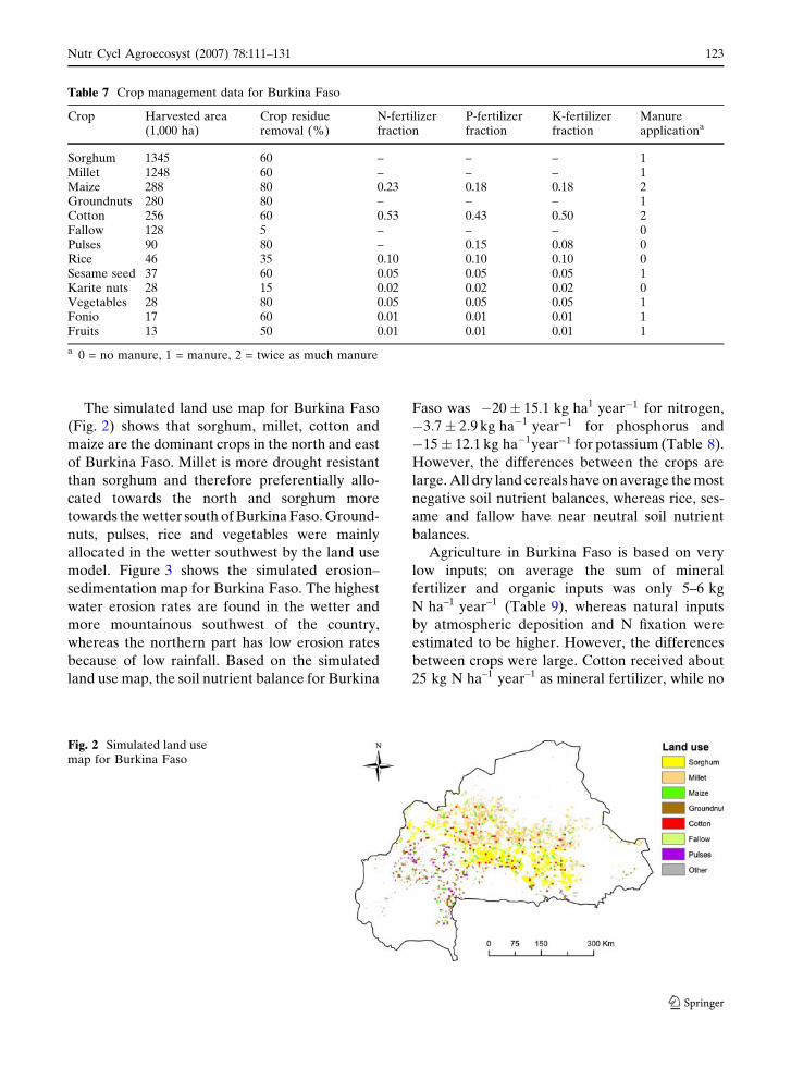
The simulated land use map for Burkina Faso

(Fig. 2) shows that sorghum, millet, cotton and

maize are the dominant crops in the north and east

of Burkina Faso. Millet is more drought resistant

than sorghum and therefore preferentially allo-

cated towards the north and sorghum more

towards the wetter south of Burkina Faso. Ground-

nuts, pulses, rice and vegetables were mainly

allocated in the wetter southwest by the land use

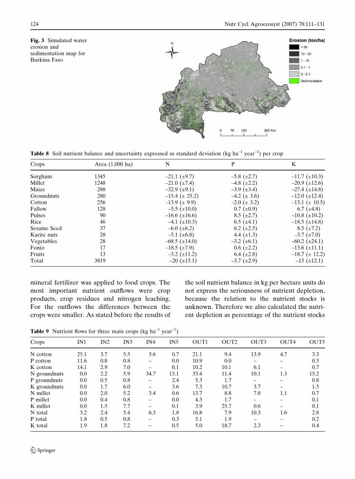
model. Figure 3 shows the simulated erosion–

sedimentation map for Burkina Faso. The highest

water erosion rates are found in the wetter and

more mountainous southwest of the country,

whereas the northern part has low erosion rates

because of low rainfall. Based on the simulated

land use map, the soil nutrient balance for Burkina

Faso was �20� 15:1 kg ha1 year�1 for nitrogen,

�3:7� 2:9 kg ha�1 year�1 for phosphorus and

�15� 12:1 kg ha�1year�1 for potassium (Table 8).

However, the differences between the crops are

large. All dry land cereals have on average the most

negative soil nutrient balances, whereas rice, ses-

ame and fallow have near neutral soil nutrient

balances.

Agriculture in Burkina Faso is based on very

low inputs; on average the sum of mineral

fertilizer and organic inputs was only 5–6 kg

N ha–1 year–1 (Table 9), whereas natural inputs

by atmospheric deposition and N fixation were

estimated to be higher. However, the differences

between crops were large. Cotton received about

25 kg N ha–1 year–1 as mineral fertilizer, while no

Table 7 Crop management data for Burkina Faso

Crop Harvested area(1,000 ha)

Crop residueremoval (%)

N-fertilizerfraction

P-fertilizerfraction

K-fertilizerfraction

Manureapplicationa

Sorghum 1345 60 – – – 1Millet 1248 60 – – – 1Maize 288 80 0.23 0.18 0.18 2Groundnuts 280 80 – – – 1Cotton 256 60 0.53 0.43 0.50 2Fallow 128 5 – – – 0Pulses 90 80 – 0.15 0.08 0Rice 46 35 0.10 0.10 0.10 0Sesame seed 37 60 0.05 0.05 0.05 1Karite nuts 28 15 0.02 0.02 0.02 0Vegetables 28 80 0.05 0.05 0.05 1Fonio 17 60 0.01 0.01 0.01 1Fruits 13 50 0.01 0.01 0.01 1

a 0 = no manure, 1 = manure, 2 = twice as much manure

Fig. 2 Simulated land usemap for Burkina Faso


123

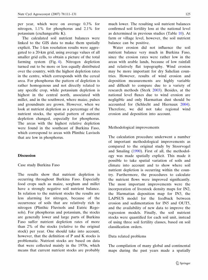
mineral fertilizer was applied to food crops. The

most important nutrient outflows were crop

products, crop residues and nitrogen leaching.

For the outflows the differences between the

crops were smaller. As stated before the results of

the soil nutrient balance in kg per hectare units do

not express the seriousness of nutrient depletion,

because the relation to the nutrient stocks is

unknown. Therefore we also calculated the nutri-

ent depletion as percentage of the nutrient stocks

Fig. 3 Simulated watererosion andsedimentation map forBurkina Faso

Table 8 Soil nutrient balance and uncertainty expressed as standard deviation (kg ha–1 year–1) per crop

Crops Area (1,000 ha) N P K

Sorghum 1345 –21.1 (±9.7) –5.8 (±2.7) –11.7 (±10.3)Millet 1248 –21.0 (±7.4) –4.8 (±2.2) –20.9 (±12.6)Maize 288 –32.9 (±9.1) –3.9 (±3.4) –27.4 (±14.8)Groundnuts 280 –15.4 (± 25.2) –4.2 (± 3.6) –12.0 (±12.4)Cotton 256 –13.9 (± 9.9) –2.0 (± 3.2) –13.1 (± 10.5)Fallow 128 –5.5 (±10.0) 0.7 (±0.9) 6.7 (±4.8)Pulses 90 –16.6 (±16.6) 8.5 (±2.7) –10.8 (±10.2)Rice 46 –4.1 (±10.3) 6.5 (±4.1) –18.5 (±14.8)Sesame Seed 37 –6.0 (±6.2) 6.2 (±2.5) 8.5 (±7.2)Karite nuts 28 –5.1 (±6.8) 4.4 (±1.3) –3.7 (±7.0)Vegetables 28 –68.5 (±14.0) –3.2 (±6.1) –60.2 (±24.1)Fonio 17 –18.5 (±7.9) 0.6 (±2.2) –13.6 (±11.1)Fruits 13 –3.2 (±11.2) 6.4 (±2.8) –18.7 (± 12.2)Total 3819 –20 (±15.1) –3.7 (±2.9) –15 (±12.1)

Table 9 Nutrient flows for three main crops (kg ha–1 year–1)

Crops IN1 IN2 IN3 IN4 IN5 OUT1 OUT2 OUT3 OUT4 OUT5

N cotton 25.1 3.7 5.5 3.6 0.7 21.1 9.4 13.9 4.7 3.3P cotton 11.6 0.8 0.8 – 0.0 10.9 0.0 – – 0.3K cotton 14.1 2.9 7.0 – 0.1 10.2 10.1 6.1 – 0.7N groundnuts 0.0 2.2 5.9 34.7 13.1 33.4 11.4 10.1 1.3 15.2P groundnuts 0.0 0.5 0.8 – 2.4 5.3 1.7 – – 0.8K groundnuts 0.0 1.7 6.0 – 3.6 7.3 10.7 3.7 – 1.5N millet 0.0 2.0 5.2 3.4 0.6 13.7 8.8 7.8 1.1 0.7P millet 0.0 0.4 0.8 – 0.0 4.3 1.7 – – 0.1K millet 0.0 1.5 7.7 – 0.1 3.9 25.7 0.6 – 0.1N total 3.2 2.4 5.4 6.3 1.8 16.8 7.9 10.3 1.6 2.8P total 1.8 0.5 0.8 – 0.3 5.1 1.9 – – 0.2K total 1.9 1.8 7.2 – 0.5 5.0 18.7 2.3 – 0.4


123

per year, which were on average 0.3% for

nitrogen, 1.1% for phosphorus and 2.1% for

potassium (exchangeable K).

The calculated soil nutrient balances were

linked to the GIS data to make them spatially

explicit. The 1-km resolution results were aggre-

gated to a 20-km grid, using average values of all

smaller grid cells, to obtain a picture of the total

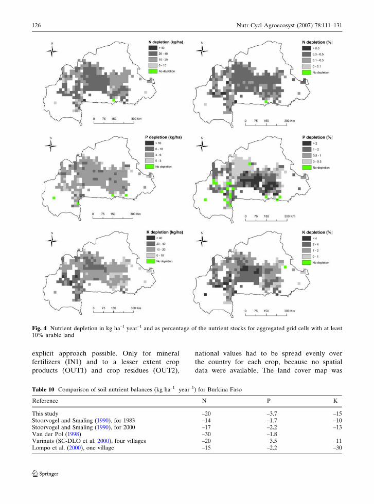
farming system (Fig. 4). Nitrogen depletion

turned out to be more or less equally distributed

over the country, with the highest depletion rates

in the centre, which corresponds with the cereal

area. For phosphorus the pattern of depletion is

rather homogenous and not directly related to

any specific crop, while potassium depletion is

highest in the central north, associated with

millet, and in the southwest, where maize, pulses

and groundnuts are grown. However, when we

look at nutrient depletion as a percentage of the

nutrient stocks, the spatial pattern of nutrient

depletion changed, especially for phosphorus.

The areas with the highest relative depletion

were found in the southeast of Burkina Faso,

which correspond to areas with Plinthic Luvisols

that are low in phosphorus.

Discussion

Case study Burkina Faso

The results show that nutrient depletion is

occurring throughout Burkina Faso. Especially

food crops such as maize, sorghum and millet

have a strongly negative soil nutrient balance.

In relation to the nutrient stocks the results are

less alarming for nitrogen, because of the

occurrence of soils that are relatively rich in

nitrogen (Plinthic Fluvisols and Eutric Rego-

sols). For phosphorus and potassium, the stocks

are generally lower and large parts of Burkina

Faso suffer nutrient depletion rates of more

than 2% of the stocks (relative to the original

stock) per year. One should take into account,

however, that the definition of P and K stocks is

problematic. Nutrient stocks are based on data

that were collected mainly in the 1970s, which

means that current nutrient stocks are probably

much lower. The resulting soil nutrient balances

confirmed soil fertility loss at the national level

as determined in previous studies (Table 10). At

farm or village level, however, the soil nutrient

balance can be positive.

Water erosion did not influence the soil

nutrient balance very much in Burkina Faso,

since the erosion rates were rather low in the

areas with arable lands, because of low rainfall

and relatively flat topography. Wind erosion

may be more important for dry Sahelian coun-

tries. However, results of wind erosion and

deposition measurements are highly variable

and difficult to compare due to a variety of

research methods (Sterk 2003). Besides, at the

national level fluxes due to wind erosion are

negligible and only Harmattan dust should be

accounted for (Schlecht and Hiernaux 2004).

Therefore, we did not take regional wind

erosion and deposition into account.

Methodological improvements

The calculation procedure underwent a number

of important methodological improvements as

compared to the original study by Stoorvogel

and Smaling (1990). First of all, the methodol-

ogy was made spatially explicit. This made it

possible to take spatial variation of soils and

climate into account and to show where soil

nutrient depletion is occurring within the coun-

try. Furthermore, the procedures to calculate

the nutrient flows were improved significantly.

The most important improvements were the

incorporation of livestock density maps for IN2,

the Harmattan deposition map for IN3, the

LAPSUS model for the feedback between

erosion and sedimentation for IN5 and OUT5,

and the availability of new data to improve the

regression models. Finally, the soil nutrient

stocks were quantified for each soil unit, instead

of using three soil fertility classes, based on soil

classification orders.

Data related problems

The compilation of many global and continental

maps during the past years made a spatially


123

explicit approach possible. Only for mineral

fertilizers (IN1) and to a lesser extent crop

products (OUT1) and crop residues (OUT2),

national values had to be spread evenly over

the country for each crop, because no spatial

data were available. The land cover map was

Fig. 4 Nutrient depletion in kg ha–1 year–1 and as percentage of the nutrient stocks for aggregated grid cells with at least10% arable land

Table 10 Comparison of soil nutrient balances (kg ha–1 year–1) for Burkina Faso

Reference N P K

This study –20 –3.7 –15Stoorvogel and Smaling (1990), for 1983 –14 –1.7 –10Stoorvogel and Smaling (1990), for 2000 –17 –2.2 –13Van der Pol (1998) –30 –1.8Varinuts (SC-DLO et al. 2000), four villages –20 3.5 11Lompo et al. (2000), one village –15 –2.2 –30


123

based on satellite images of 1992–1993 that

were classified without elaborate ground tru-

thing. The map shows little cultivated land on

the border between the semi-arid and sub-

humid zones, which coincides with the south

and southwest of Burkina Faso, while long-term

field observations show that cultivation is com-

mon and covers large areas (Kruska et al. 2003).

The classified map should therefore be con-

firmed by local field checks, but this has hardly

been done for the African continent.

Next to spatial data, tabular data also differ

in quality. For example, FAOSTAT crop data

are based on sample surveys and not on total

census data, while livestock data are normally

better registered and available as total census

data. Another point of attention is the use of

regression models, which are supposed not to be

used outside their own boundaries. However,

due to limited datasets the boundaries do not

cover the whole range of African conditions of

soils, climate and management. The N leaching

regression model had boundaries of 40–

2,000 mm rainfall, 3–54% clay content and

0.25–2 m layer thickness (De Willigen 2000).

For the K leaching regression model less data

was available, which limited the borders to 1.3–

8.1 cmol/kg for CEC, 211–2420 mm for rainfall

and 0–273 kg ha–1 for the amount of fertilizer.

Besides, most of these experiments were fertil-

izer trials, in which more than average fertilizer

was applied.

Land use map

The land use map was based on crop suitabilities,

which means that crops with high requirements

were allocated to the best locations and that crops

with low requirements were used to fill up remain-

ing grid cells. This should be the expected situation,

but will be beside reality, because of socio-eco-

nomic, demographic and political drivers (Steph-

enne and Lambin 2001). Multiple and inter

cropping systems could not be simulated, because

each land unit could only be allocated to one crop.

However, the regional distribution of crops was

more important than the accuracy of individual

grid cells, because the results were aggregated

afterwards to 20-km grid cells. Satellite images

classified according to land use, i.e., crop distribu-

tion, would be an improvement. New initiatives,

such as Africover (www.africover.org), offer an

alternative for the simulated land use map. This

multi-purpose land cover database is based on

better and newer satellite images, has been thor-

oughly checked in the field and has a more specific

legend. However, this map still does not distinguish

individual crops or fallow periods but cropping

systems and is only available for ten East-African

countries up to now.

Erosion modelling

The quantitative results of erosion modelling with

the LAPSUS model have to be treated with care.

The model was developed at watershed level

(25 m grid cell resolution) while we used it at the

national level (1 km grid cell resolution). This

means that topography is not correctly repre-

sented at the watershed scale, because small

valleys and ridges are levelled out (Temme et al.

2006). Nevertheless, the erosion–sedimentation

patterns appear to be simulated well, although

verification at this scale level is hardly possible. A

factor that is not included in the model but which

affects erosion is agricultural land management

(Schoorl and Veldkamp 2001). However, this

could not be incorporated at this scale, because

this is highly variable between farmers and no data

at national level are available. Nevertheless, the

LAPSUS model is so far the only model that can

simulate erosion and sedimentation in a dynamic

way and in quantitative terms at this scale.

Uncertainty assessment

The uncertainty assessment showed that the total

uncertainty of the soil nutrient balances was

relatively low, compared to the uncertainties of

all input data. The uncertainties demonstrate that

for most crops soil nutrient depletion is a fact. The

uncertainty analysis also showed that cross and

spatial correlations between the various nutrient

flows and uncertainties affect the total uncertainty

of the nutrient balance. However, a more rigorous

uncertainty analysis is required to gain more

confidence in the outcomes. Questions that need

to be addresses in further studies are: (i) how


123

realistic are the assumptions, (ii) which assump-

tions and uncertainties can be improved and (iii)

what is the sensitivity of the uncertainty assessment

and the spatial aggregation procedure. It should

also be noted that in the uncertainty analysis we did

not pay attention to the effect of model error,

which potentially is an important source of error.

However, assessment of model error was beyond

the scope of this study.

Concluding remarks

For these results to become more meaningful at a

policy and private sector level, it is useful to

downscale them to specific regions (e.g., cotton-

based, livestock-based, millet-based), as was done

for Mali, Ghana and Kenya (FAO 2004). Policy

interventions to replenish soil fertility should take

place at this so-called meso-level, which is suffi-

ciently large to provide benefits for all farmers and

small enough to target local policies that deal with

local conditions. It also allows recognition of areas

that managed to bounce back after a period of

degradation, such as parts of the Mossi Plateau in

Burkina Faso (Reij and Thiombiano 2003). How-

ever, FAO (2004) showed that at this level the

availability of data, and especially spatial data, is

problematic and often national data and maps have

to be used. Therefore, the results of the soil

nutrient balances at the national level offer a good

starting point to target soil fertility policies at the

lower level. One can choose a crop/farming system

or a specific region where soil fertility decline is

most pronounced or threatening farmers’ income

or food security. Besides, the spatially explicit

soil nutrient balances at the national level offer

the possibility for extrapolation of soil fertility

research that was successful at the district or village

level.

The nutrient balance is only an indicator of

sustainability as far as soil fertility (management)

is concerned; it does not reveal ‘best practices’

that make prevailing or alternative agro-ecosys-

tems more sustainable. A functional link with

nutrient stocks, farming systems, and integrated

nutrient management systems is needed (Smaling

and Dixon 2006). Results presented in kg ha–1 do

not offer direct entry points for intervention and

are not very meaningful for policy makers. They

prefer outcomes in terms of yield loss or mone-

tary values. A next step is therefore the linkage of

soil nutrient balances to other tools and data to

widen its use, e.g., a simple crop production

model to express soil nutrient depletion in terms

of yield losses. Other attractive indicators to

possibly attach to the soil nutrient balance are the

nutritive value of diets and food and cash need.

Up to now the soil nutrient balance was presented

as a static tool, which calculated soil nutrient

balances for a specific year. The next step is to

create a dynamic soil nutrient balance model,

linked to a land use change model, which includes

changes in land use and land management. The

temporal dimension of such a model will improve

the results, especially for dynamic farming systems.

Acknowledgements This paper is based on a studycommissioned by the Land and Water DevelopmentDivision (AGLL) of the Food and AgricultureOrganization of the United Nations (FAO), andpublished under the title Scaling Soil Nutrient Balances(FAO 2004). Jan Poulisse and Tanja van den Bergen ofAGLL are gratefully acknowledged for their support.

References

Alexandratos N (ed) (1988) World agriculture: toward2000, an FAO study. Belhaven Press, London

Allen RG, Pereira LS, Raes D, Smith M (1998) Cropevapotranspiration – guidelines for computing cropwater requirements. FAO Irrigation and drainagepaper 56. FAO, Rome

Baijukya FP, Steenhuijsen de Piters B (1998) Nutrientbalances and their consequences in the banana-basedland use systems of Bukoba district, northwest Tan-zania. Agr Ecosyst Environ. 71:147–158

Batjes NH (2002) Soil parameter estimates for the soiltypes of the world for use in global and regionalmodelling (version 2.0). ISRIC report 2002/02. ISRIC,Wageningen, The Netherlands

Baudet GJR, Yoboue V, Lacaux JP (1989) Etude desapports humides de certains elements chimiques dansla foret dense de Cote d’Ivoire

Bindraban PS, Stoorvogel JJ, Jansen DM, VlamingJ, Groot JRR (2000) Land quality indicators forsustainable land management: proposed method foryield gap and soil nutrient balance. Agr EcosystEnviron 81:103–112

Bond DW, Steiger S, Zhang RY, Tie XX, Orville RE(2002) The importance of NOx production by light-ning in the tropics. Atmos Environ 36(9):1509–1519

Bouwman AF (1998) Nitrogen oxides and tropical agri-culture. Nature 392:866–867


123

Bruijnzeel LA (1990) Hydrology of moist tropical forestsand effects of conversion: a state of knowledgereview. Free University, Amsterdam

Budelman A, Defoer T (2000) Managing soil fertilityin the tropics—PLAR and resource flow analysisin practice. Case studies from Benin, Ethiopia,Kenya, Mali and Tanzania. Royal Tropical Institute,Amsterdam

Camara OS (1996) Utilisation des residus de recolte et dufumier dans le Cercle de Koutiala: Bilan des elementsnutritifs et analyse economique. Rapport PSS No. 18.AB-DLO, Wageningen, The Netherlands

Cogle AL, Roa KPC, Yule DF, Smith GD, George PJ,Srinivasan ST, Jangawad L (2002) Soil managementfor Alfisols in the semiarid tropics: erosion,enrichment factors and runoff. Soil Use Manage18:10–17

Danso SKA (1992) Biological nitrogen fixation in tropicalagroecosystems: twenty years of biological nitrogenfixation research in Africa. In: Mulongoy K, Gueye M,Spencer DSC (eds) Biological nitrogen fixation andsustainability of tropical agriculture. John Wiley SonsLtd, Chichester, UK

De Koning GHJ, Van den Kop PJ, Fresco LO (1997)Estimates of sub-national nutrient balances as sus-tainability indicators for agro-ecosystems in Ecua-dor. Agr Ecosyst Environ 65:127–139

De Willigen P (2000) An analysis of the calculation ofleaching and denitrification losses as practised in theNUTMON approach. Report 18. Plant ResearchInternational, Wageningen, The Netherlands

Dixon J, Gulliver A, Gibbon D (2001) Global farmingsystems study: challenges and priorities to 2030.Synthesis and global overview. FAO, Rome

Doll P, Siebert S (2000) A digital global map of irrigatedareas. ICID J 49(2):55–66

Drees LR, Manu A, Wilding LP (1993) Characteristics ofaeolian dusts in Niger, West Africa. Geoderma59:213–233

Faerge J, Magid J (2004) Evaluating NUTMON nutrientbalancing in Sub-Saharan Africa. Nut Cycl Agro69:101–110

FAO (1976) A Framework for land evaluation. SoilsBulletin 32. FAO, Rome

FAO (1978) Report on the agro-ecological zones project.Vol. 1-Methodology and results for Africa. World SoilResources Report 48, FAO, Rome

FAO/UNESCO (1997) Digital soil map of the world andderived soil properties. Land and water digital mediaseries no 1. FAO, Rome

FAO (1998) ECOCROP 1, 2—The crop environmentalrequirements database and the crop environmentresponse database. Land and water digital mediaseries no 4. FAO, Rome

FAO and IIASA (2000) Global agro-ecological zones.Land and water digital media series no 11. FAO,Rome

FAO (2001) Lecture notes on the major soils of the world.World soil resources report no 94. FAO, Rome

FAO (2003) FAOSTAT agriculture data. FAO, Rome

FAO (2004) Scaling soil nutrient balances—enablingmesoscale approaches for African realities. FAOfertilizer and plant nutrition bulletin 15. FAO, Rome

Folmer ECR, Geurts PMH, Francisco JR (1998) Assess-ment of soil fertility depletion in Mozambique. AgrEcosyst Environ 71:159–167

Foster GR, Meyer LD (1975) Mathematical simulation ofupland erosion by fundamental erosion mechanics. In:Anonymous (ed) Present and perspective technologyfor predicting sediment yields and sources. Proceed-ings sediment yield workshop, Oxford, 1972, Depart-ment of Agriculture, Washington, DC

Fox J, Krummel J, Yarnasarn S, Ekasingh M, Podger N(1995) Land-use and landscape dynamics in northernThailand—assessing chang in 3 upland watershed.Ambio 24:328–334

Fernandez-Rivera S, Williams TO, Hiernaux P, Powell JM(1995) Faecal excretion by ruminants and manureavailability for crop production in semi-arid WestAfrica. In: Powell JM, Fernandez-Rivera S, WilliamsTO, Renard C (eds) Livestock and sustainable nutri-ent cycling in mixed farming systems of sub-SaharanAfrica. Volume II: technical Papers. InternationalLivestock Centre for Africa (ILCA), Addis Ababa

Giller KE (2001) Nitrogen fixation in tropical croppingsystems, 2nd edn. CABI Publishing, Wallingford, UK

Giller KE, Wilson KJ (1991) Nitrogen fixation in tropicalcropping systems. CAB International, Wallingford,UK

Hartemink AE (2003) Soil fertility decline in the tropicswith case studies on plantations. CABI Publishing,Wallingford, UK

Heuvelink GBM (1998) Uncertainty analysis in environ-mental modelling under a change of spatial scale. NutCycl Agro 50:255–264

Heuvelink GBM (1999) Aggregation and error propaga-tion in GIS. In: Lowell K, Jaton A (eds), Spatialaccuracy assessment. Land information uncertainty innatural resources. Ann Arbor Press, Chelsea, US

IFA/FAO (2001) Global estimates of gaseous emissions ofNH3, NO and N2O from agricultural land. FAO,Rome

IFA/IFDC/FAO (2000) Fertilizer use by crop. 4th edn.FAO, Rome

IPCC (1997) Revised 1996 IPCC guidelines for nationalgreenhouse gas inventories. Reference manual (Vol-ume 3)

Jones MJ, Bromfield AR (1970) Nitrogen in the rainfall atSamaru, Nigeria. Nature 227:86

Kalu AE (1979) The African dust plume: its characteristicsand propagation across West Africa in winter. In:Morales C (ed) Saharan Dust: Mobilization, Trans-port, Deposition. SCOPE Report 14. John Wiley andSons, Chichester, UK

Khisa P, Gachene CKK, Karanja NK, Mureithi JG (2002)The effect of post-harvest crop cover on soil erosionin a maize-legume based cropping system in Gatanga,Kenya. J Agric Trop Subtrop 103(1):17–28

Kirkby MJ (1986) A two-dimensional simulation model forslope and stream evolution. In: Abrahams AD (ed)


123

Hillslope processes. Allen & Unwin Inc, Winchester,US

Kruska RL, Reis RS, Thornton PK, Henninger N, Krist-janson PM (2003) Mapping livestock-oriented agri-cultural production systems for the developing world.Agr Syst 77:39–63

Langdon JR (1991) Booker tropical soil manual Ahandbook for soil survey and agricultural land eval-uation in the tropics and subtropics. Longman GroupUN Ltd, Essex, UK

Langenberg VT, Nyamushahu S, Roijackers R, KoelmansAA (2002) Assessing external nutrient sources forLake Tanganyika. Wageningen University, Wagenin-gen, The Netherlands

Leemans R, Cramer W (1991) The IIASA database formean monthly values of temperature, precipitationand cloudiness on a global terrestrial grid. Researchreport RR-91–18. International Institute of AppliedSystems Analysis, Laxenburg, Austria

Lekasi JK, Tanner JC, Kimani SK, Harris PJC (2001)Managing manure to sustain smallholder livelihoodsin the east African highlands. Kenya AgriculturalResearch Institute, Nairobi

Lompo F, Bonzi M, Zougmore R, Youl S (2000) Reha-bilitation of soil fertility in Burkina Faso. In: HilhorstT, Muchena FM (eds) Nutrients on the move—soilfertility dynamics in African farming systems. Inter-national Institute for Environment and Development,London

McTainsh GH (1980) Harmattan dust deposition innorthern Nigeria. Nature 286:587–588

McTainsh GH, Walker PH (1982) Nature and distributionof Harmattan dust. Z Geomor NF 26:417–435

Meyer J, Pampfer E (1959) Nitrogen content of rain watercollected in the humid central Congo basin. Nature184:717–718

Moberg JP, Esu IE, Malgwi WB (1991) Characteristics andconstituent composition of Harmattan dust falling inNorthern Nigeria. Geoderma 48:73–91

Oenema O, Heinen M (1999) Uncertainties in nutrientbudgets due to biases and errors. In: Smaling EMA,Oenema O, Fresco LO (eds) Nutrient disequilibria inagroecosystems—concepts and case studies. CABIPublishing, Wallingford, UK

Pieri C (1985) Bilans mineraux des systemes de culturespluviales en zones arides et semi-arides. L’AgronTrop 40:1–20

Priess JA, De Koning GHJ, Veldkamp A (2001) Assess-ment of interactions between land use change andcarbon and nutrient fluxes in Ecuador. Agr EcosystEnviron. 85: 269–279

Pye K (1987) Aeolian dust and dust deposits. AcademicPress Limited, London,

Roy RN, Misra RV, Lesschen JP, Smaling EMA (2003)Assessment of soil nutrient balance. Approaches andmethodologies. FAO Fertilizer and plant nutritionbulletins 14. FAO, Rome

Reij C, Thiombiano T (2003) Developpement ruralet environnement au Burkina Faso: la rehabilitationde la capacite productive des terroirs sur la partienord du Plateau Central entre 1980 et 2001.

Rapport de synthese. DGIS/Netherlands Embassy,Ouagadougou

Richard C (1963) Pluviometrie et etude physico-chimiquedes eaux de pluie-Addis-Abeba. L’Agron Trop:1073–1080

SC-DLO, CIRAD-CA, INERA, NAGREF, KARI (2000)VARINUTS Spatial and temporal variation of soilnutrient stocks and management in sub-SaharanAfrican farming systems. Final report. SC-DLO,Wageningen, The Netherlands

Schlecht E, Mahler F, Sangare M, Susenbeth A, Becker K(1995) Quantitative and qualitative estimation ofnutrient intake and faecal excretion of zebu cattlegrazing natural pasture in semi-arid Mali. In: PowellJM, Fernandez-Rivera S, Williams TO, Renard C(eds) Livestock and sustainable nutrient cycling inmixed farming systems of sub-Saharan Africa. Vol-ume II: technical papers. International LivestockCentre for Africa (ILCA), Addis Ababa

Schlecht E, Hiernaux P (2004) Beyond adding up inputand outputs: process assessment and upscaling inmodelling nutrient flows. Nut Cycl Agro 70:303–319

Schoorl JM, Veldkamp A (2001) Linking land use andlandscape process modelling: a case study for theAlora region (South Spain). Agr Ecosyst Environ85:281–293

Schoorl JM, Veldkamp A, Bouma J (2002) Modellingwater and soil redistribution in a dynamic landscapecontext. Soil Sci Soc Am J 66:1610–1619

Schoorl JM, Boix Fayos C, De Meijer RJ, van der GraafER, Veldkamp A (2004) The 137Cs technique on steepMediterranean slopes (Part II): landscape evolutionand model calibration. Catena 57(1):35–54

Schulze R (2000) Transcending scales of space and time inimpact studies of climate and climate change onagrohydrological responses. Agr Ecosyst Environ82:185–212

Scoones I, Toulmin C (1998) Soil nutrient balances: whatuse for policy? Agr Ecosyst Environ 71:255–267

Smaling EMA, Dixon J, (2006) Adding a soil fertilitydimension to global farming system approach, withcases from Africa. Agr Ecosyst Environ 116:15–26

Smaling EMA, Oenema O, Fresco LO (eds) (1999)Nutrient disequilibria in agroecosystems—Conceptsand case studies. CABI Publishing, Wallingford,UK

Stephenne N, Lambin EF (2001) A dynamic simulationmodel of land-use changes in Dusano-sahelian coun-tires of Africa (SALU). Agr Ecosyst Environ 85:145–161

Sterk G (2003) Causes, consequences and control of winderosion in Sahelian Africa: a review. Land DegradDev 14:95–108

Stocking M (1984) Erosion and soil productivity: a review.Consultants’ working paper no. 1. AGLS. FAO,Rome

Stocking M (1986) The cost of soil erosion in Zimbabwe interms of the loss of three major nutrient. Consultants’working paper no. 3. AGLS. FAO, Rome

Stoorvogel JJ, Smaling EMA (1990) Assessment of soilnutrient depletion in sub-Saharan Africa: 1983–2000.


123

Report 28. Winand Staring Centre, Wageningen, TheNetherlands

Stoorvogel JJ, Smaling EMA, Janssen BH (1993) Calcu-lating soil nutrient balances in Africa at differentscales. 1. Supra-national scale. Fert Res 35: 227–235

Stoorvogel JJ, van Breemen N, Janssen BH (1997a) Thenutrient input by Harmattan dust to a forest ecosystemin Cote d’Ivoire, Africa. Biogeochemistry 37:145–157

Stoorvogel JJ, Janssen BH, Van Breemen N (1997b) Thenutrient budgets of a watershed and its forest ecosys-tem in the Tai National Park in Cote d’Ivoire.Biogeochemistry 37:159–172

Temme A, Schoorl JM, Veldkamp A (2006) An algorithmto deal with depressions in dynamic landscape evolu-tion models. Comput Geosci 32:452–461

Tiessen H, Hauffe HK, Mermut AR (1991) Deposition ofHarmattan dust and its influence on base saturation ofsoils in northern Ghana. Geoderma 49:285–299

US Geological Survey (USGS), University of Nebraska-Lincoln and European Commission’s Joint ResearchCentre (2000) Africa land cover characteristics data

base. Version 2.0. Seasonal land cover region legend.USGS, Sioux Falls, US

US Geological Survey (USGS) (1998) Hydro 1K Africa.Elevation data. USGS, Sioux Falls, US

Van der Pol F (1998) Gestion de la fertilite des terres along terme dans les pays du CILSS. Unpublishedreport. KIT, Amsterdam

Williams TO, Powell JM, Fernandez-Rivera S (1995)Manure utilisation, drought cycles and herd dynamicsin the Sahel: implications for cropland productivity.In: Powell JM, Fernandez-Rivera S, Williams TO,Renard C (eds) Livestock and sustainable nutrientcycling in mixed farming systems of sub-SaharanAfrica. Vol. II: technical papers. International Live-stock Centre for Africa (ILCA), Addis Ababa

Wint W, Slingenbergh J, Rogers D (2000) Livestockdistribution, production and diseases: towards a globallivestock atlas. Consultants’ report. FAO, Rome

World Bank (2005) World Development Indicators 2005,Washington DC


123

a spatially explicit methodology to quantify soil nutrient ...late soil nutrient balances in a...

Documents