a review on efficacious methods to decolorize reactive azo dye
TRANSCRIPT

EDITORIAL TEAM
Editors Celso Augusto Guimarães Santos, Federal University of Paraíba, Brazil Masuo Kashiwadani, Ehime University, Japan Dragan Savic, University of Exeter, United Kingdom Vicente L. Lopes, Texas State University, United States Richarde Marques da Silva, Federal University of Paraíba, Brazil
Associate Editors Koichi Suzuki, Niihama National College of Technology, Japan Hafzullah Aksoy, Istanbul Technical University, Turkey António Pais Antunes, University of Coimbra, Portugal Roberto Leal Pimentel, Federal University of Paraíba, Brazil Max Billib, Hannover University, Germany Bernardo Arantes do Nascimento Teixeira, Federal University of São Carlos, Brazil Generoso de Angelis Neto, State University of Maringá, Brazil
FOCUS and SCOPE
Journal of Urban and Environmental Engineering (JUEE) provides a forum for original papers and for the exchange of information and views on significant developments in urban and environmental engineering worldwide. The scope of the
journal includes:
(a) Water Resources and Waste Management: This topic includes (i) waste and sanitation; (ii) environmental
issues; (iii) the hydrological cycle on the Earth; (iv) surface water, groundwater, snow and ice, in all their physical,
chemical and biological processes, their interrelationships, and their relationships to geographical factors, atmospheric processes and climate, and Earth processes including erosion and sedimentation; (v) hydrological extremes and their
impacts; (vi) measurement, mathematical representation and computational aspects of hydrological processes; (vii)
hydrological aspects of the use and management of water resources and their change under the influence of human
activity; (viii) water resources systems, including the planning, engineering, management and economic aspects of
applied hydrology.
(b) Constructions and Environment: Buildings and infrastructure constructions (bridges/footbridges, pipelines etc)
are part of every urban area. In recent years there is a growing interest in seeking rationality of construction systems, in
balance with environmental adequacy and harmony in an urban area. This involves, among others, adequacy of structural
systems (shapes, functionality, rational design etc), use of alternative materials for construction (recycled,
environmentally friendly materials etc) and solutions seeking energy efficiency.
(c) Urban Design: This topic covers the arrangement, appearance and functionality of towns and cities, and in
particular the shaping and uses of urban public space (e.g. streets, plazas, parks and public infrastructure), including also
urban planning, landscape architecture, or architecture issues (e.g. thermic and acoustic comfort).
(d) Transportation Engineering: This topic covers such area as Traffic & Transport Management, Rail Transport, Air
Transport, International Transport, Logistics/Physical Distribution/Supply Chain Management, Management Information Systems & Computer Applications, Motor Transport, Regulation/Law, Transport Policy, and Water Transport.
SUMMARY
EVALUATION OF THE STORM EVENT MODEL DWSM ON A MEDIUM-SIZED WATERSHED IN CENTRAL NEW YORK, USA
Peng Gao, Deva K. Borah, Maria Josefson
DEVELOPING SUSTAINABILITY INDICATORS FOR WATER RESOURCES MANAGEMENT IN TIETÊ-JACARÉ BASIN, BRAZIL Michele Almeida Corrêa, Bernardo Arantes do Nascimento Teixeira
EVALUATION OF NEW TOWNS CONSTRUCTION IN THE AROUND OF TEHRAN MEGACITIY Nader Zali, Sajjad Hatamzadeh, Seyed Reza Azadeh, Taravat Ershadi Salmani
ARSENIC CONTAMINATION IN GROUNDWATER: A STATISTICAL MODELING Palas Roy, Naba Kumar Mondal, Biswajit Das, Kousik Das
A REVIEW ON EFFICACIOUS METHODS TO DECOLORIZE REACTIVE AZO DYE Josephraj Vijayaraghavan, S. J. Sardhar Basha, Joe Jegan
MATHEMATICAL MODEL FOR THE SIMULATION OF WATER QUALITY IN RIVERS USING THE VENSIM PLE® SOFTWARE
Julio Cesar Souza Inácio Gonçalves; Marcius F. Giorgetti
URBAN SPRAWL IN SMALL CITIES, ANALYSIS OF THE MUNICIPALITY OF SÃO PEDRO (SP): POTENTIALS AND CONSTRAINS
Priscila Carrara Fracassi, José Augusto Lollo
A REVIEW ON EFFICACIOUS METHODS TO DECOLORIZE REACTIVE AZO DYE Sivaraja Subramania Pillai, Ryuichiro Yoshie
URBAN GROWTH AND WATER QUALITY IN THIMPHU, BHUTAN Nandu Giri, O. P. Singh
MANAGING PHYSICAL DEVELOPMENT IN PERI-URBAN AREAS OF KUMASI, GHANA: A CASE OF ABUAKWA
Paul Amoateng, Patrick Brandful Cobbinah, Kwasi Owusu-Adade
BIOGAS POTENTIAL OF ORGANIC WASTE IN NIGERIA Chima Ngumah, Jude N. Ogbulie, Justina C. Orji, Ekpewerechi S. Amadi
OPERATIONAL PERFORMANCE OF VERTICAL UPFLOW ROUGHING FILTER FOR PRE-TREATMENT OF LEACHATE USING LIMESTONE FILTER MEDIA
Augustine Chioma Affam
PERFORMANCE ANALYSIS OF A HELICAL SAVONIUS ROTOR WITHOUT SHAFT AT 45° TWIST ANGLE USING CFD
Bachu Deb, Rajat Gupta, R.D. Misra
EFFECTIVENESS OF WASTE STABILIZATION PONDS IN REMOVAL OF LINEAR ALKYL BENZENE SALFONATE (LAS)
Ahmad Mohmed Abdelrahman, Ahmed Mohmed, Ali Gad, Mohmed Hashem
THE ACTORS OF A WIND POWER CLUSTER: A CASE OF A WIND POWER CAPITAL Jari Matti Sarja
FLOW PHYSICS OF 3-BLADED STRAIGHT CHORD H-DARRIEUS WIND TURBINE Rajat Gupta, Agnimitra Biswas
ANAEROBIC EFFLUENT POST-TREATMENT APPLYING PHOTOLYTIC REACTOR PRIOR TO AGRICULTURAL USE IN BRAZILIAN'S SEMIARID REGION
José Tavares Sousa, Geralda Lima, Wilton Silva Lopes, Eclésio Cavalcante Santo, José Lima Oliveira Júnior
RETROFITTING OF REINFORCED CONCRETE BEAMS USING FIBRE REINFORCED POLYMER (FRP) COMPOSITES – A REVIEW
Namasivayam Aravind, Amiya K. Samanta, D. K. Singha Roy, Joseph V. Thanikal KOHONEN NEURAL NETWORKS FOR RAINFALL-RUNOFF MODELING: CASE STUDY OF PIANCÓ RIVER BASIN Camilo A. S. Farias, Celso A. G. Santos, Artur M. G. Lourenço and Tatiane C. Carneiro AN ANALYSIS OF REGIONAL DISPARITIES SITUATION IN THE EAST AZARBAIJAN PROVINCE OF IRANNader Zali, Hassan Ahmadi, Seyed Mohammadreza Faroughi
Gao, Borah and Josefson
Journal of Urban and Environmental Engineering (JUEE), v.7, n.1, p.1-7, 2013
1
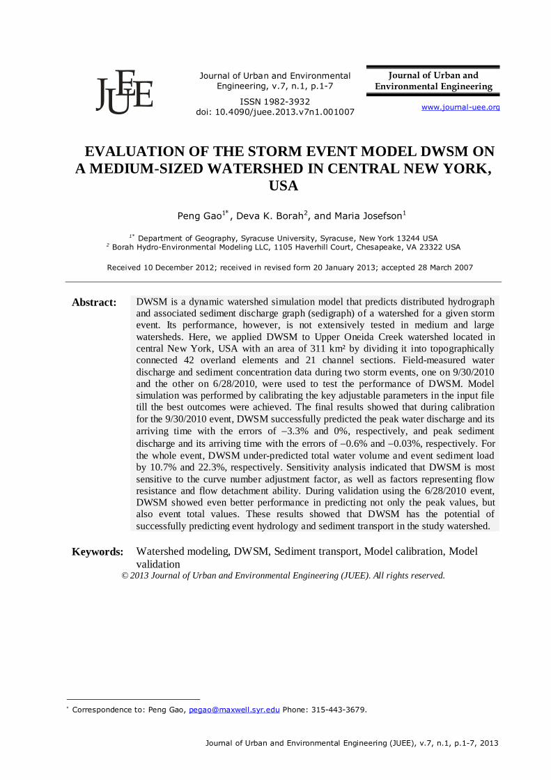
Journal of Urban and Environmental Engineering, v.7, n.1, p.1-7
Journal of Urban and Environmental Engineering
UEEJ ISSN 1982-3932
doi: 10.4090/juee.2013.v7n1.001007 www.journal-uee.org
EVALUATION OF THE STORM EVENT MODEL DWSM ON A MEDIUM-SIZED WATERSHED IN CENTRAL NEW YORK,
USA
Peng Gao1, Deva K. Borah2, and Maria Josefson1
1* Department of Geography, Syracuse University, Syracuse, New York 13244 USA 2 Borah Hydro-Environmental Modeling LLC, 1105 Haverhill Court, Chesapeake, VA 23322 USA
Received 10 December 2012; received in revised form 20 January 2013; accepted 28 March 2007
Abstract: DWSM is a dynamic watershed simulation model that predicts distributed hydrograph
and associated sediment discharge graph (sedigraph) of a watershed for a given storm event. Its performance, however, is not extensively tested in medium and large watersheds. Here, we applied DWSM to Upper Oneida Creek watershed located in central New York, USA with an area of 311 km² by dividing it into topographically connected 42 overland elements and 21 channel sections. Field-measured water discharge and sediment concentration data during two storm events, one on 9/30/2010 and the other on 6/28/2010, were used to test the performance of DWSM. Model simulation was performed by calibrating the key adjustable parameters in the input file till the best outcomes were achieved. The final results showed that during calibration for the 9/30/2010 event, DWSM successfully predicted the peak water discharge and its arriving time with the errors of 3.3% and 0%, respectively, and peak sediment discharge and its arriving time with the errors of 0.6% and 0.03%, respectively. For the whole event, DWSM under-predicted total water volume and event sediment load by 10.7% and 22.3%, respectively. Sensitivity analysis indicated that DWSM is most sensitive to the curve number adjustment factor, as well as factors representing flow resistance and flow detachment ability. During validation using the 6/28/2010 event, DWSM showed even better performance in predicting not only the peak values, but also event total values. These results showed that DWSM has the potential of successfully predicting event hydrology and sediment transport in the study watershed.
Keywords:
Watershed modeling, DWSM, Sediment transport, Model calibration, Model validation
© 2013 Journal of Urban and Environmental Engineering (JUEE). All rights reserved.
Correspondence to: Peng Gao, [email protected] Phone: 315-443-3679.
Gao, Borah and Josefson
Journal of Urban and Environmental Engineering (JUEE), v.7, n.1, p.1-7, 2013
2
INTRODUCTION
The complex transport processes of suspended sediment at the watershed scale may be more efficiently characterized by physically-based watershed models (Borah and Bera, 2004; Singh and Frebert, 2006). Among various existing watershed models, Dynamic Watershed Simulation Model (DWSM) is the one of relatively high efficiency with a relatively simple model structure that involves a set of overland elements and the connected stream segments (Borah, 2011; Borah and Bera, 2004). It uses several mathematical equations to characterize various surface and subsurface hydrological processes, and sediment entrainment and transport processes both on hillslopes and in stream channels during a single rainfall event. Spatial variations of topographic, soil, and land use and land cover characteristics are simplified by assigning single values to each of the divided elements. By routing water and sediment discharges through the divided elements, DWSM predicts both hydrograph and sediment discharge graph (sedigraph) of the watershed at the outlet for a given rainfall event. Although DWSM has been very successful in predicting suspended sediment transport during storms of small watersheds (Borah et al., 2002), it has not been widely tested for watersheds with relatively big sizes in various climatic regions. In this study, we applied DWSM to a medium-size watershed in central New York, USA. Using measured data of water discharge and sediment concentrations for two events of 2010 (one in summer and the other in fall), we tested its abilities of predicting (1) peak water and sediment discharges and (2) event total water volume and sediment yield, and performed sensitivity analysis for the key adjustable model parameters to investigate the behavior of DWSM in the study watershed.
METHOD Study watershed Oneida Creek watershed is one of seven sub-watersheds discharging to Oneida Lake of central New York, USA. Its main stream, Oneida Creek originates from the southwestern side of the watershed, flows southeast and then turns to north till reaching Oneida Lake (Fig. 1). Its main tributary, Sconondoa Creek extends upstream to the southeast of the watershed. Topographically, the downstream part of the watershed is quite flat, while the middle- and upper-stream ones vary greatly in elevations ranging approximately from 120 to 570 m.
The Oneida creek watershed has a typical continental climate with moderate temperatures and rainfalls in summers and cold, intensive snowfalls in winter. Its
mean annual precipitation is more than 1270 mm. With more than half of the area used for agriculture (e.g., dairy farms and cultivated lands) and urbanization, the watershed supplies significantly high sediment loads than other sub-watersheds to Oneida Lake and serves as the main source of sediment pollution to the Lake. Quantifying sediment load and its variation is essential for the design and implementation of sediment-related best management practices (BMP). The middle and upper sections of the Oneida Creek watershed were selected as the study watershed (Fig. 1) to take advantage of hydrological data available in a gauging station established by United State Geological Survey (USGS) near the outlet and to capture the topographic diversity of the area. The study watershed has the area of 311 km2, and thus is a medium-sized watershed (Singh, 1995).
Data preparation Stage recording and water sampling were performed through a long-term monitoring station established at the outlet of the study watershed. The monitoring station involves an automatic pumping sampler installed at the outlet of the study watershed that consists of a marine battery to supply power to the sampler, a pressure transducer to record stages of the flowing water, and a sampling tube to collect suspended sediment samples by sucking sediment-laden water into a series of 24 sample bottles.
The stages of the flow were constantly recorded at 15-minute intervals. When a pre-determined threshold value of flow stage was exceeded, the sampler began to collect sediment-laden flow samples every three or four hours and stopped when the stage dropped below the threshold at the end of the rainfall event.
Fig. 1 The studied watershed
Gao, Borah and Josefson
Journal of Urban and Environmental Engineering (JUEE), v.7, n.1, p.1-7, 2013
3
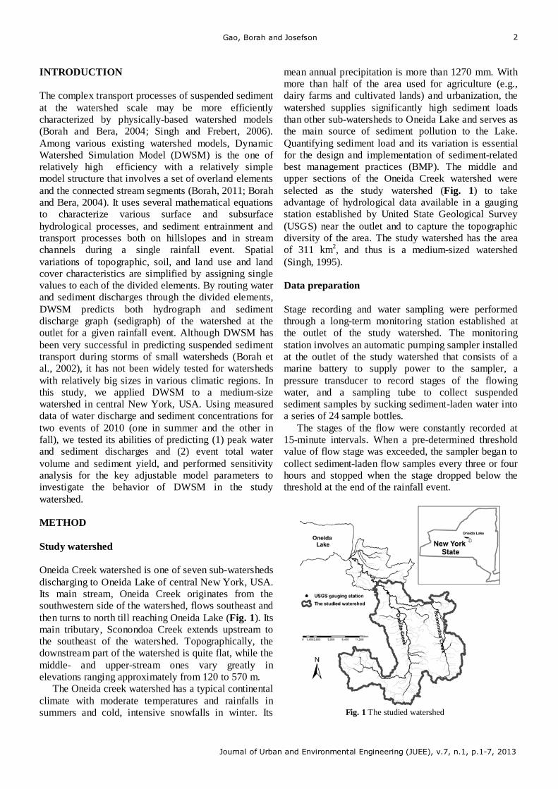
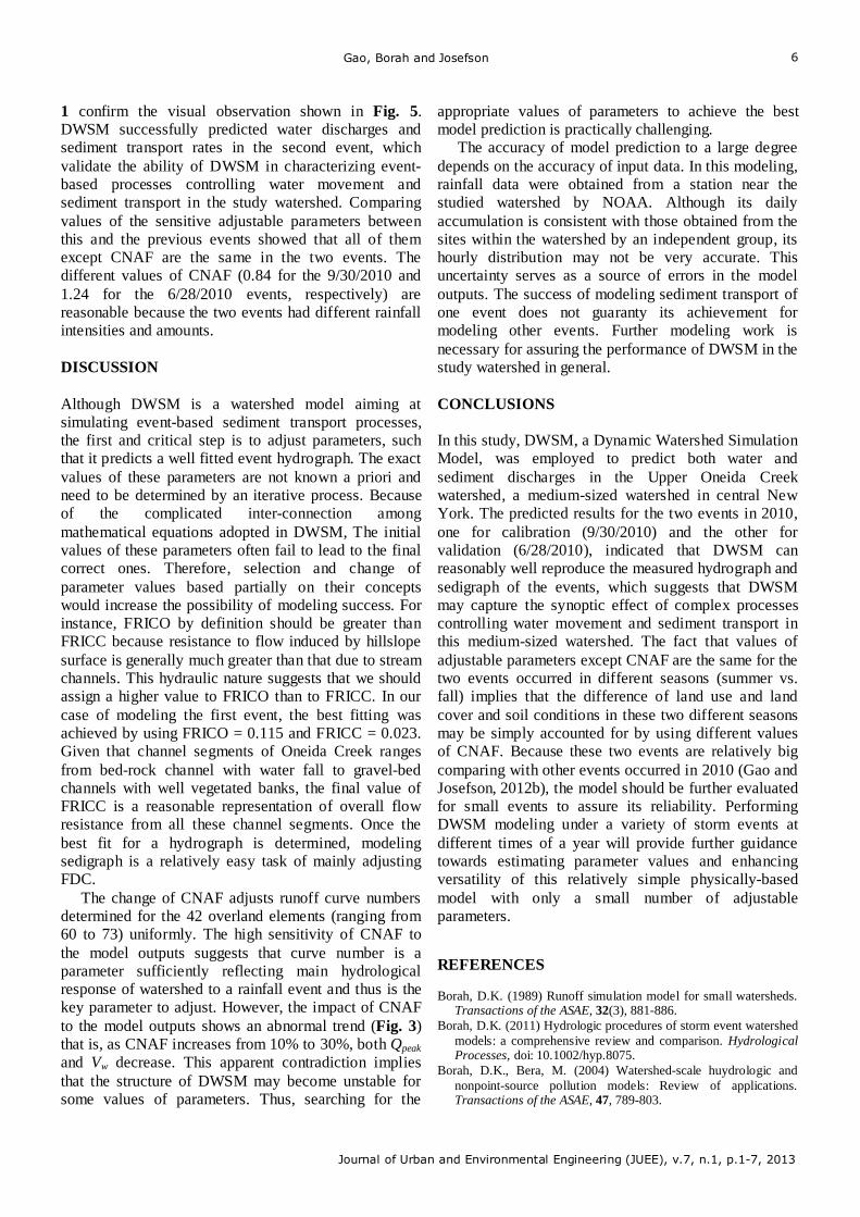
Fig. 2 Comparison of measured with modeled hydrograph and
sedigraph of the 9/30/2010 event
The samples were subsequently taken back to the
Physical Geography Laboratory at Syracuse University for analysis to obtain sediment concentrations (C). Water discharges (Q; hydrograph) of the event were determined in terms of the correlation between measured Q at the outlet and the associated Q recorded at the USGS gauging station (Fig. 1). A sediment rating curve was subsequently established using the measured pairs of C and Q. Sediment discharge, Qs, was then calculated by Qs = QC and used to determine the event sediment yield by summing Qs over the time period of the event (Gao and Josefson, 2012a).
The study watershed was spatially divided into 42 overland elements and 21 stream segments using the ArcHydro technique (Maidment, 2002) for modeling. Each element or segment was assigned a set of parameters to represent its physiographic and land use and land cover (LULC) conditions. The basic input parameters, such as slope and slope length, overland area, and stream segment length were determined based on the DEM data with the resolution of 10 × 10 meter. Soil and LULC parameters were determined using GIS in terms of available GIS layers. Four different median sizes of sediment fractions and their corresponding percentages were determined based on particle size analysis for several samples collected at the outlet of the studied watershed. These values were entered into the input data file. Rainfall information of the modeled events was obtained from the National Oceanic and Atmospheric Administration (NOAA) website by email request. Model calibration and validation were performed by adjusting a set of parameters that will be elaborated in the sensitivity analysis section.
DWSM has two different methods of simulating rainfall excess. The first is the SCS runoff curve number (CN) procedure in which the rainfall excess (direct runoff rate) is calculated from CN values of overland
elements and breakpoint cumulative precipitation data (Borah 1989). The second is the interception-infiltration procedure in which the rate of rainfall excess is calculated by subtracting rainfall losses in interception (both tree canopies and ground covers) and infiltration from rainfall intensity (Borah et al., 2002). The first method has been commonly and successfully used in modeling both Q and Qs because of its simplicity and hence is adopted in this study. Using the prepared input data, DWSM was conducted to predict the hydrograph and the corresponding sedigraph of the selected events that can fit observed ones as accurate as possible. RESULTS Model calibration
The September 30, 2010 storm event generated a single-mode hydrograph with peak water discharge (Qpeak) of 85.35 m3/s (Fig. 2). The modeled Qpeak value is 88.15 m3/s, 3.3% higher than the measured one. The predicted arriving time of Qpeak is only 15 minute later than the measured one. Associated with the hydrograph is a single-mode sedigraph with the peak sediment discharge (Qspeak) of 89.29 kg/s. The modeled Qspeak value is 89.76 kg/s, merely 0.6% more than the measured one. Furthermore, the modeled arriving time Qspeak is one hour earlier than the measured one. These results demonstrated clearly that DWSM is capable of simulating both magnitude and timing of Qpeak and Qspeak.
The modeled rising limb of the hydrograph is steeper than the measured one, while the modeled falling limb follows along the measured one first and then decreases with a gentler slope than the measured one giving rise to higher predicted Q values than the measured ones toward the end. Overall, the total volume of storm water (Vw) generated by the event is 8.38 × 10⁶ m3 whereas the modeled one is 7.49 × 10⁶ m3, about 10.7% less than the measured one. This under-estimation is mainly caused by the delayed but fast increased storm flows predicted by DWSM during the rising limb of the event. Nonetheless, the small predicted percent errors for Qpeak and Vw further indicates that DWSM successfully captures the hydrological behavior of the storm event.
Simulated sediment discharge values generally agreed well with the measured ones. The under-estimation over the lower section of the rising limb is primarily caused by the under-estimation of Q during the same period. Although DWSM correctly predicts Qspeak both in magnitude and timing, it does not simulate sediment discharge values very well for the earlier section of the falling limb (Fig. 4). However, the predicted event sediment yield, SSYe is 4465 ton, which is only 22.3% less than the measured SSYe (5748 ton).
Gao, Borah and Josefson
Journal of Urban and Environmental Engineering (JUEE), v.7, n.1, p.1-7, 2013
4
Given the complexity of sediment transport processes, this predicting error is very well acceptable. These results showed that DWSM correctly characterizes physical processes controlling water movement and suspended sediment transport in the study watershed and hence is capable of predicting both Qspeak and SSYe. Sensitivity analysis In the DWSM input file, there are two types of parameters. The first are those determined in terms of watershed topographical features, channel morphology, and sediment information, such as slope length and area of overland element or channel segment, coefficients of the relationship between wetted perimeter and flow area, and percentages of sediment sizes in three different ranges. These parameters are not adjustable once determined. The second are those representing watershed surface conditions, land use and land cover, and soil characteristics, such as uniform curve number adjustment factor for model calibration (CNAF), Manning’s roughness coefficient of overland and channel (FRICO and FRICC), and interception storage capacity for a typical ground cover (VOG). These parameters are adjustable. Modeling event-based hydrological response and sediment transport is essentially identifying a set of values for these parameters that can generate the results best fit the measured Q and Qs values. Therefore, understanding the sensitivity of these parameters to the predicted hydrological and sediment values is critical for examining the predictability of DWSM.
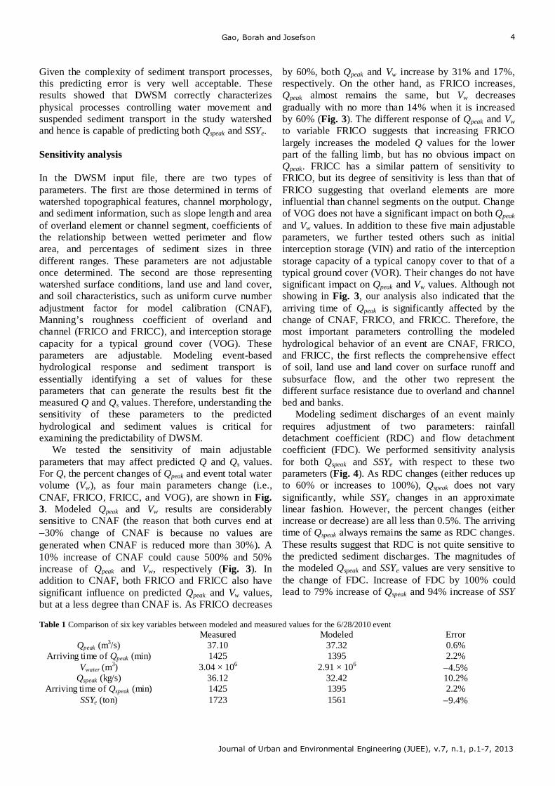
We tested the sensitivity of main adjustable parameters that may affect predicted Q and Qs values. For Q, the percent changes of Qpeak and event total water volume (Vw), as four main parameters change (i.e., CNAF, FRICO, FRICC, and VOG), are shown in Fig. 3. Modeled Qpeak and Vw results are considerably sensitive to CNAF (the reason that both curves end at 30% change of CNAF is because no values are generated when CNAF is reduced more than 30%). A 10% increase of CNAF could cause 500% and 50% increase of Qpeak and Vw, respectively (Fig. 3). In addition to CNAF, both FRICO and FRICC also have significant influence on predicted Qpeak and Vw values, but at a less degree than CNAF is. As FRICO decreases
by 60%, both Qpeak and Vw increase by 31% and 17%, respectively. On the other hand, as FRICO increases, Qpeak almost remains the same, but Vw decreases gradually with no more than 14% when it is increased by 60% (Fig. 3). The different response of Qpeak and Vw to variable FRICO suggests that increasing FRICO largely increases the modeled Q values for the lower part of the falling limb, but has no obvious impact on Qpeak. FRICC has a similar pattern of sensitivity to FRICO, but its degree of sensitivity is less than that of FRICO suggesting that overland elements are more influential than channel segments on the output. Change of VOG does not have a significant impact on both Qpeak and Vw values. In addition to these five main adjustable parameters, we further tested others such as initial interception storage (VIN) and ratio of the interception storage capacity of a typical canopy cover to that of a typical ground cover (VOR). Their changes do not have significant impact on Qpeak and Vw values. Although not showing in Fig. 3, our analysis also indicated that the arriving time of Qpeak is significantly affected by the change of CNAF, FRICO, and FRICC. Therefore, the most important parameters controlling the modeled hydrological behavior of an event are CNAF, FRICO, and FRICC, the first reflects the comprehensive effect of soil, land use and land cover on surface runoff and subsurface flow, and the other two represent the different surface resistance due to overland and channel bed and banks.
Modeling sediment discharges of an event mainly requires adjustment of two parameters: rainfall detachment coefficient (RDC) and flow detachment coefficient (FDC). We performed sensitivity analysis for both Qspeak and SSYe with respect to these two parameters (Fig. 4). As RDC changes (either reduces up to 60% or increases to 100%), Qspeak does not vary significantly, while SSYe changes in an approximate linear fashion. However, the percent changes (either increase or decrease) are all less than 0.5%. The arriving time of Qspeak always remains the same as RDC changes. These results suggest that RDC is not quite sensitive to the predicted sediment discharges. The magnitudes of the modeled Qspeak and SSYe values are very sensitive to the change of FDC. Increase of FDC by 100% could lead to 79% increase of Qspeak and 94% increase of SSY
Table 1 Comparison of six key variables between modeled and measured values for the 6/28/2010 event
Measured Modeled Error Qpeak (m
3/s) 37.10 37.32 0.6% Arriving time of Qpeak (min) 1425 1395 2.2%
Vwater (m3) 3.04 × 10⁶ 2.91 × 10⁶ 4.5%
Qspeak (kg/s) 36.12 32.42 10.2% Arriving time of Qspeak (min) 1425 1395 2.2%
SSYe (ton) 1723 1561 9.4%
Gao, Borah and Josefson
Journal of Urban and Environmental Engineering (JUEE), v.7, n.1, p.1-7, 2013
5
(a)
(b)
Fig. 3 Hydrological sensitivity analysis for the four main parameters.
(a) Qpeak; (b) Vw.
Fig. 4 Sediment sensitivity analysis for the two relevant parameters
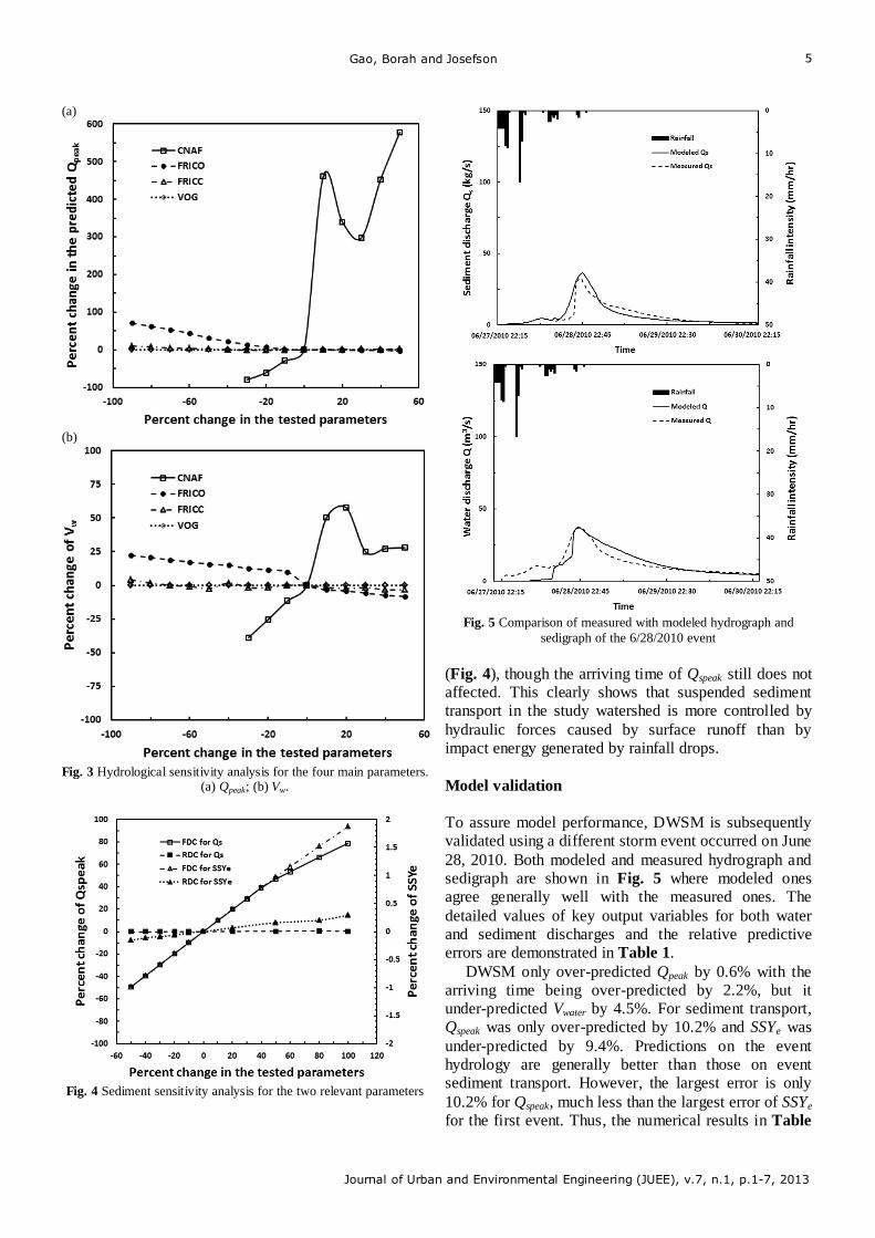
Fig. 5 Comparison of measured with modeled hydrograph and
sedigraph of the 6/28/2010 event
(Fig. 4), though the arriving time of Qspeak still does not affected. This clearly shows that suspended sediment transport in the study watershed is more controlled by hydraulic forces caused by surface runoff than by impact energy generated by rainfall drops. Model validation To assure model performance, DWSM is subsequently validated using a different storm event occurred on June 28, 2010. Both modeled and measured hydrograph and sedigraph are shown in Fig. 5 where modeled ones agree generally well with the measured ones. The detailed values of key output variables for both water and sediment discharges and the relative predictive errors are demonstrated in Table 1.
DWSM only over-predicted Qpeak by 0.6% with the arriving time being over-predicted by 2.2%, but it under-predicted Vwater by 4.5%. For sediment transport, Qspeak was only over-predicted by 10.2% and SSYe was under-predicted by 9.4%. Predictions on the event hydrology are generally better than those on event sediment transport. However, the largest error is only 10.2% for Qspeak, much less than the largest error of SSYe for the first event. Thus, the numerical results in Table
Gao, Borah and Josefson
Journal of Urban and Environmental Engineering (JUEE), v.7, n.1, p.1-7, 2013
6
1 confirm the visual observation shown in Fig. 5. DWSM successfully predicted water discharges and sediment transport rates in the second event, which validate the ability of DWSM in characterizing event-based processes controlling water movement and sediment transport in the study watershed. Comparing values of the sensitive adjustable parameters between this and the previous events showed that all of them except CNAF are the same in the two events. The different values of CNAF (0.84 for the 9/30/2010 and 1.24 for the 6/28/2010 events, respectively) are reasonable because the two events had different rainfall intensities and amounts. DISCUSSION
Although DWSM is a watershed model aiming at simulating event-based sediment transport processes, the first and critical step is to adjust parameters, such that it predicts a well fitted event hydrograph. The exact values of these parameters are not known a priori and need to be determined by an iterative process. Because of the complicated inter-connection among mathematical equations adopted in DWSM, The initial values of these parameters often fail to lead to the final correct ones. Therefore, selection and change of parameter values based partially on their concepts would increase the possibility of modeling success. For instance, FRICO by definition should be greater than FRICC because resistance to flow induced by hillslope surface is generally much greater than that due to stream channels. This hydraulic nature suggests that we should assign a higher value to FRICO than to FRICC. In our case of modeling the first event, the best fitting was achieved by using FRICO = 0.115 and FRICC = 0.023. Given that channel segments of Oneida Creek ranges from bed-rock channel with water fall to gravel-bed channels with well vegetated banks, the final value of FRICC is a reasonable representation of overall flow resistance from all these channel segments. Once the best fit for a hydrograph is determined, modeling sedigraph is a relatively easy task of mainly adjusting FDC.
The change of CNAF adjusts runoff curve numbers determined for the 42 overland elements (ranging from 60 to 73) uniformly. The high sensitivity of CNAF to the model outputs suggests that curve number is a parameter sufficiently reflecting main hydrological response of watershed to a rainfall event and thus is the key parameter to adjust. However, the impact of CNAF to the model outputs shows an abnormal trend (Fig. 3) that is, as CNAF increases from 10% to 30%, both Qpeak and Vw decrease. This apparent contradiction implies that the structure of DWSM may become unstable for some values of parameters. Thus, searching for the
appropriate values of parameters to achieve the best model prediction is practically challenging.
The accuracy of model prediction to a large degree depends on the accuracy of input data. In this modeling, rainfall data were obtained from a station near the studied watershed by NOAA. Although its daily accumulation is consistent with those obtained from the sites within the watershed by an independent group, its hourly distribution may not be very accurate. This uncertainty serves as a source of errors in the model outputs. The success of modeling sediment transport of one event does not guaranty its achievement for modeling other events. Further modeling work is necessary for assuring the performance of DWSM in the study watershed in general. CONCLUSIONS
In this study, DWSM, a Dynamic Watershed Simulation Model, was employed to predict both water and sediment discharges in the Upper Oneida Creek watershed, a medium-sized watershed in central New York. The predicted results for the two events in 2010, one for calibration (9/30/2010) and the other for validation (6/28/2010), indicated that DWSM can reasonably well reproduce the measured hydrograph and sedigraph of the events, which suggests that DWSM may capture the synoptic effect of complex processes controlling water movement and sediment transport in this medium-sized watershed. The fact that values of adjustable parameters except CNAF are the same for the two events occurred in different seasons (summer vs. fall) implies that the difference of land use and land cover and soil conditions in these two different seasons may be simply accounted for by using different values of CNAF. Because these two events are relatively big comparing with other events occurred in 2010 (Gao and Josefson, 2012b), the model should be further evaluated for small events to assure its reliability. Performing DWSM modeling under a variety of storm events at different times of a year will provide further guidance towards estimating parameter values and enhancing versatility of this relatively simple physically-based model with only a small number of adjustable parameters.
REFERENCES Borah, D.K. (1989) Runoff simulation model for small watersheds.
Transactions of the ASAE, 32(3), 881-886. Borah, D.K. (2011) Hydrologic procedures of storm event watershed
models: a comprehensive review and comparison. Hydrological Processes, doi: 10.1002/hyp.8075.
Borah, D.K., Bera, M. (2004) Watershed-scale huydrologic and nonpoint-source pollution models: Review of applications. Transactions of the ASAE, 47, 789-803.

Gao, Borah and Josefson
Journal of Urban and Environmental Engineering (JUEE), v.7, n.1, p.1-7, 2013
7
Borah, D. K., Xia, R., Bera, M. (2002) DWSM - a dynamic watershed simulation model. Mathematical models of small watershed hydrology and applications, in Mathematical models of small watershed hydrology and applications, edited by V. P. Singh and D. Frevert, Water Resources Publications, LLC., Highlands Ranch, Colorado, 113-166.
Gao, P., Josefson, M. (2012a) Event-based suspended sediment dynamics in a central New York watershed. Geomorphology, 139-140, 425-437.
Gao, P. and Josefson, M. (2012b) Temporal variations of suspended sediment transport in Oneida Creek watershed, Central New York. J. Hydrol 426-427, 17-27.
Maidment, D.R. (2002). Arc Hydro, GIS for Water Resources, ESRI, Redland, 203p.
Singh, V.P. (1995) Watershed modeling, in Computer models of watershed hydrology, edited by V. P. Singh, Water Resources Publications, Littleton, CO, 1-22.
Singh, V.P., Frebert, D.K. (2006) Watershed models, Talyor & Francis, Boca Raton, 653p.

Corrêa and Teixeira
Journal of Urban and Environmental Engineering (JUEE), v.7, n.1, p.8-14, 2013
8
Journal of Urban and Environmental Engineering, v.7, n.1, p.8-14
Journal of Urban and Environmental Engineering
UEEJ ISSN 1982-3932
doi: 10.4090/juee.2013.v7n1.008014 www.journal-uee.org
DEVELOPING SUSTAINABILITY INDICATORS FOR WATER RESOURCES MANAGEMENT IN TIETÊ-JACARÉ
BASIN, BRAZIL
Michele de Almeida Corrêa1 and Bernardo Arantes do Nascimento Teixeira1 1 Graduate Program in Urban Engineering, Federal University of São Carlos, Brazil
Received 5 March 2012; received in revised form 19 January 2013; accepted 30 January 2013
Abstract: This paper describes a tool to assist in developing water resources management,
focusing on the sustainability concept, by a Basin Committee. This tool consists of a set of sustainability indicators for water resources management denominated CISGRH, which was identified by a conceptual and empirical review to meet the specific needs of the study herein - the basin committee of Tietê-Jacaré Rivers (CBH-TJ). The framework of CISGRH came about through consecutive consultation processes. In the first consultation, the priority problems were identified for the study objectives, listing some possible management sustainability indicators. These preliminary indicators were also submitted to academic specialists and technicians working in CBH-TJ for a new consultation process. After these consultation stages, the CISGRH analysis and structuring were introduced. To verify the indicators’ adaptation and to compose a group as proposed by the study, these were classified according to specific sustainability principles for water resources management. The objective of the CISGRH implementation is to diagnose current conditions of water resources and its management, as well as to evaluate future conditions evidenced by tendencies and interventions undertaken by the committee.
Keywords:
Water resources management; sustainable development; basin committee.
© 2013 Journal of Urban and Environmental Engineering (JUEE). All rights reserved.
Correspondence to: Michele de Almeida Corrêa, Tel.: +55 14 9703 4815; E-mail: [email protected]
Corrêa and Teixeira
Journal of Urban and Environmental Engineering (JUEE), v.7, n.1, p.8-14, 2013
9
INTRODUCTION In Brazil, water resources management has been frequently discussed in the last years, addressing, for example: (a) the 1934 Water Code promulgation (Ordinance No.
24.643 of July 10, 1934) with a centralized view on some sections, mainly the electric power generation section;
(b) the Brazilian Constitution of 1988, that stipulated the institution of a National System of Water Resources Management; and
(c) the Water Resources National Politics in 1997 (Federal Law No. 9.433, BRASIL, 1997), the latter responsible for instituting effective legal instruments in Brazil, as transcribed below.
In agreement with Article 5 of the Water Resources
National Politics, the instruments of the Water Resources National Policies are: (a) Water Resources Plans; (b) Formulating water bodies in classes, according to
the importance of water use; (c) Grants rights for the use of water resources; (d) Levy collection for the use of water resources; (e) Compensation to municipal districts; (f) Water Resources Information System.
The use of river basins as water resource management units is foreseen as one of the foundations for the Water Resources National Policy (Federal Law No. 9.433/1997) and also as one of the principles of the State Policy for Water Resources in São Paulo State (State Law No. 7.663, SÃO PAULO, 1991). Monitoring water resources management is also contemplated in these legal instruments.
In 2007, the Environment Ministry of Brazil (MMA), the Water National Agency – ANA, also a Brazilian agency, and the United Nations Program for the Environment - PNUMA launched the first publication of the global project of environmental evaluations, denominated GEO (Global Environment Outlook), created by PNUMA in 1995.
This publication, denominated GEO Brazil: Water Resources (MMA, 2007), helps to understand and evaluate the concepts and foundations, as well as the agency’s framework, legal instruments, and other water resources management instruments, which comprise the National System of Water Resources Management (denominated SINGREH).
Some of the structural problems detailed in MMA (2007) are: disorganization in the legislation of water resources and in the juridical-administrative substratum; deep-rooted difficulties correlated to the administrative culture of the State; standstill situations related to the
domain of rivers; and deviations of concepts and fundamentals that should guide the implementation of SINGREH, with a greater focus on implementing management instruments.
The document also introduces suggestions and questions to improve the water resources management process, seeking, among other aspects, to increase the participation of civil society and users of water, and to consolidate proposals that should be assessed within the scope of the basin committee.
The publication of Water Resources Conjuncture in Brazil (ANA, 2009), requested by the Water Resources National Council (denominated CNRH) through the resolution no. 58/2006, promoted a progress analysis of water resources management and the evaluation of recently implemented instruments as proposed in the Water Resources National Policies.
The conclusions of the Water Resources Conjuncture in Brazil (ANA, 2009) emphasize the need of considering the planning as a continuous process of perception, listening, interactions and concretizing the opportunities and effectuation of the plan by means of negotiation and a participative management.
It emphasizes that this is the responsibility of the Basins Committees, the monitoring actions proposed in the State’s Plans and in the Basin’s Plans through instruments not mentioned in the applicable legislation, but that can be annually reported, presenting data on: the quality and amount of water resources; and evaluation of the implemented programs foreseen in the aforementioned plans, as well as adjustment proposals.
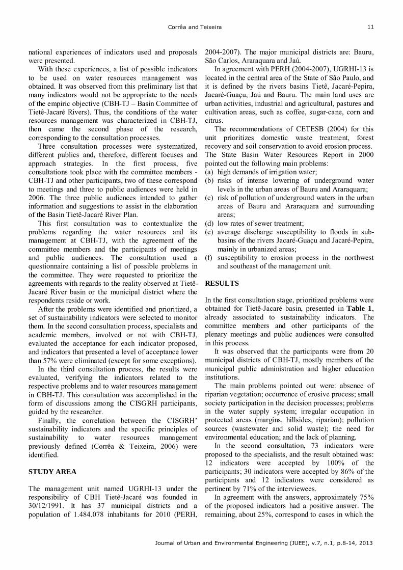
Figure 1 presents the situation of the Brazilian states concerning the institution of basin committees, as shown the home page of the Basin Committee (www.cbh.gov.br) in 2010.
Fig. 1 Number of Committees according to the Brazilian States. Abbreviations of Brazilian States: AC: Acre; AL: Alagoas; AP: Amapá; AM: Amazonas; BA: Bahia; CE: Ceará; DF: Distrito Federal; ES: Espírito Santo; GO: Goiás; MA: Maranhão; MT: Mato Grosso; MS: Mato Grosso do Sul; MG: Minas Gerais; PA: Pará; PB: Paraíba; PR: Paraná; PE: Pernambuco; PI: Piauí; RJ: Rio de Janeiro; RN: Rio Grande do Norte; RS: Rio Grande do Sul; RO: Rondônia; RR: Roraima; SC: Santa Catarina; SP: São Paulo; SE: Sergipe; and TO: Tocantins.
Corrêa and Teixeira
Journal of Urban and Environmental Engineering (JUEE), v.7, n.1, p.8-14, 2013
10
This research also discussed concepts related to sustainability, from the apprehensive viewpoint with the exploratory use of the natural resources. The sustainability or sustainable development concept was discussed in several international conferences, which culminated in documents and definitions such as “Our Common Future” and “Agenda 21”.
Besides the concepts in these documents there are sustainability indicators as monitoring tools, which can be used for water resources management, as suggested at “Agenda 21”.
The indicators calculate the progress of water resources management under the optics of sustainability, observing the results of actions implemented in the basin, the water resources management unit adopted in Brazil and in the State of São Paulo, in accordance with the Federal Law no. 9.433/97 and State Law no. 7.663/91, respectively.
Tunstall and Van Bellen (2002) highlight as important indicator characteristics, the capacity to evaluate existing conditions and tendencies; the possibility to make comparisons in spacial and temporal scales, and to evaluate the conditions and tendencies in relation to goals and objectives; and the ability to supply information, conditions and tendencies. Van Bellen (2002) describes indicators as variables, in other words, a simplified representation of an attribute belonging to a system, or an abstraction of a real attribute.
For Hezri (2004), the choice of sustainability indicators should follow some criteria, as described below: (a) robustness (scientifically accepted, measurable,
sensitive to changes, the practical focus is limited to a number of themes and comparisons with the objectives, based on appropriate perspectives);
(b) democratic inclusion with all inclusive participation, including society, specialists and stakeholders; transparent, with accessible methods and explicit analysis;
(c) longevity (capacity to be repeatedly calculated, to be interactive and adaptable to change; and to have positive cost-effectiveness);
(d) relevance (institutional capacity to obtain, to maintain and to document the necessary data; assist the public and users; present simple structure; and guided by a clear view of sustainability).
Steinemann and Cavalcanti (2006) define indicators
as variables that characterize drought conditions, stating: specific values of indicators for activating drought responses. The authors used this concept for Georgia’s first state drought plan.
According to Brugmann (1997) cited at Ioris et al (2007), the sustainability in water resources management requires using indicators that can describe
and communicate conditions (with current information or of forecast of tendencies), besides proposing the necessary actions and facilitating the participation of several stakeholders in the decision process.
Thus, to verify if the indicators proposed for a certain place are enough to calculate all aspects of sustainability to this specific case, it was proposed to verify the compliance to specific principles of sustainability within the context, as systematized by Corrêa and Teixeira (2006). In the present study the specific principles of sustainability were used for water resources management in basins, as presented below. (a) Universal access to Water Resources; (b) Responsible use of Water Resources and preventive
management performance; (c) Integrated planning, systematic and including Water
Resources use considering: Economical, Social, Ecological, Political and Cultural aspects in Water Resources Management;
(d) Decentralized basins management; (e) Management participation in Water Resources; (f) International and inter-regional cooperation; (g) Organization and supply of information; (h) Economical value of Water Resources; (i) Education for Water Resources management; (j) Negotiated solution of conflicts. OBJECTIVES
The main objective of this research was the development of a group of sustainability indicators as a tool for water resources management, in the management of the basin or unit (UGRHI).
For this main objective, the specific objectives were: (a) Identify previous experiences or indicator proposals
for water resources management; (b) Identify priority problems in UGRHI Tietê-Jacaré
in the State of São Paulo - Brazil; (c) Identify and present guidelines to implement the
proposed indicators, with emphasis on UGRHI Tietê-Jacaré.
METHODOLOGY
The process to structure CISGRH was executed in three main phases. In the first phase, the conceptual base was studied, with a discussion on sustainability aspects and water resources management found in the literature and the management model adopted in Brazil and in the State of São Paulo. In this discussion, the attributions of the Basin Committee and guidelines for water resources management were analyzed. In this phase, the definitions of the general indicators and sustainability indicators were discussed and the international and
Corrêa and Teixeira
Journal of Urban and Environmental Engineering (JUEE), v.7, n.1, p.8-14, 2013
11
national experiences of indicators used and proposals were presented.
With these experiences, a list of possible indicators to be used on water resources management was obtained. It was observed from this preliminary list that many indicators would not be appropriate to the needs of the empiric objective (CBH-TJ – Basin Committee of Tietê-Jacaré Rivers). Thus, the conditions of the water resources management was characterized in CBH-TJ, then came the second phase of the research, corresponding to the consultation processes.
Three consultation processes were systematized, different publics and, therefore, different focuses and approach strategies. In the first process, five consultations took place with the committee members - CBH-TJ and other participants, two of these correspond to meetings and three to public audiences were held in 2006. The three public audiences intended to gather information and suggestions to assist in the elaboration of the Basin Tietê-Jacaré River Plan.
This first consultation was to contextualize the problems regarding the water resources and its management at CBH-TJ, with the agreement of the committee members and the participants of meetings and public audiences. The consultation used a questionnaire containing a list of possible problems in the committee. They were requested to prioritize the agreements with regards to the reality observed at Tietê-Jacaré River basin or the municipal district where the respondents reside or work.
After the problems were identified and prioritized, a set of sustainability indicators were selected to monitor them. In the second consultation process, specialists and academic members, involved or not with CBH-TJ, evaluated the acceptance for each indicator proposed, and indicators that presented a level of acceptance lower than 57% were eliminated (except for some exceptions).
In the third consultation process, the results were evaluated, verifying the indicators related to the respective problems and to water resources management in CBH-TJ. This consultation was accomplished in the form of discussions among the CISGRH participants, guided by the researcher.
Finally, the correlation between the CISGRH’ sustainability indicators and the specific principles of sustainability to water resources management previously defined (Corrêa & Teixeira, 2006) were identified.
STUDY AREA
The management unit named UGRHI-13 under the responsibility of CBH Tietê-Jacaré was founded in 30/12/1991. It has 37 municipal districts and a population of 1.484.078 inhabitants for 2010 (PERH,
2004-2007). The major municipal districts are: Bauru, São Carlos, Araraquara and Jaú.
In agreement with PERH (2004-2007), UGRHI-13 is located in the central area of the State of São Paulo, and it is defined by the rivers basins Tietê, Jacaré-Pepira, Jacaré-Guaçu, Jaú and Bauru. The main land uses are urban activities, industrial and agricultural, pastures and cultivation areas, such as coffee, sugar-cane, corn and citrus.
The recommendations of CETESB (2004) for this unit prioritizes domestic waste treatment, forest recovery and soil conservation to avoid erosion process. The State Basin Water Resources Report in 2000 pointed out the following main problems: (a) high demands of irrigation water; (b) risks of intense lowering of underground water
levels in the urban areas of Bauru and Araraquara; (c) risk of pollution of underground waters in the urban
areas of Bauru and Araraquara and surrounding areas;
(d) low rates of sewer treatment; (e) average discharge susceptibility to floods in sub-
basins of the rivers Jacaré-Guaçu and Jacaré-Pepira, mainly in urbanized areas;
(f) susceptibility to erosion process in the northwest and southeast of the management unit.
RESULTS
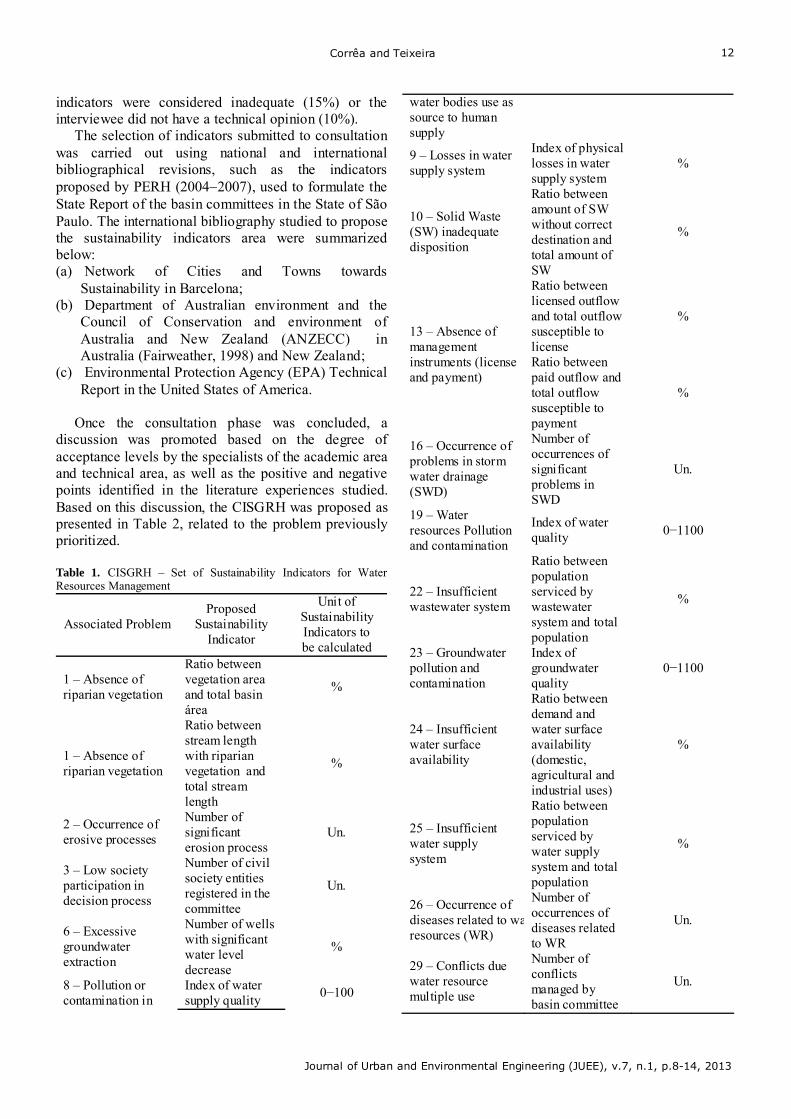
In the first consultation stage, prioritized problems were obtained for Tietê-Jacaré basin, presented in Table 1, already associated to sustainability indicators. The committee members and other participants of the plenary meetings and public audiences were consulted in this process.
It was observed that the participants were from 20 municipal districts of CBH-TJ, mostly members of the municipal public administration and higher education institutions.
The main problems pointed out were: absence of riparian vegetation; occurrence of erosive process; small society participation in the decision processes; problems in the water supply system; irregular occupation in protected areas (margins, hillsides, riparian); pollution sources (wastewater and solid waste); the need for environmental education; and the lack of planning.
In the second consultation, 73 indicators were proposed to the specialists, and the result obtained was: 12 indicators were accepted by 100% of the participants; 30 indicators were accepted by 86% of the participants and 12 indicators were considered as pertinent by 71% of the interviewees.
In agreement with the answers, approximately 75% of the proposed indicators had a positive answer. The remaining, about 25%, correspond to cases in which the
Corrêa and Teixeira
Journal of Urban and Environmental Engineering (JUEE), v.7, n.1, p.8-14, 2013
12
indicators were considered inadequate (15%) or the interviewee did not have a technical opinion (10%).
The selection of indicators submitted to consultation was carried out using national and international bibliographical revisions, such as the indicators proposed by PERH (20042007), used to formulate the State Report of the basin committees in the State of São Paulo. The international bibliography studied to propose the sustainability indicators area were summarized below: (a) Network of Cities and Towns towards
Sustainability in Barcelona; (b) Department of Australian environment and the
Council of Conservation and environment of Australia and New Zealand (ANZECC) in Australia (Fairweather, 1998) and New Zealand;
(c) Environmental Protection Agency (EPA) Technical Report in the United States of America.
Once the consultation phase was concluded, a
discussion was promoted based on the degree of acceptance levels by the specialists of the academic area and technical area, as well as the positive and negative points identified in the literature experiences studied. Based on this discussion, the CISGRH was proposed as presented in Table 2, related to the problem previously prioritized. Table 1. CISGRH – Set of Sustainability Indicators for Water Resources Management
Associated Problem Proposed
Sustainability Indicator
Unit of Sustainability Indicators to be calculated
1 – Absence of riparian vegetation
Ratio between vegetation area and total basin área
%
1 – Absence of riparian vegetation
Ratio between stream length with riparian vegetation and total stream length
%
2 – Occurrence of erosive processes
Number of significant erosion process
Un.
3 – Low society participation in decision process
Number of civil society entities registered in the committee
Un.
6 – Excessive groundwater extraction
Number of wells with significant water level decrease
%
8 – Pollution or contamination in
Index of water supply quality
0−100
water bodies use as source to human supply
9 – Losses in water supply system
Index of physical losses in water supply system
%
10 – Solid Waste (SW) inadequate disposition
Ratio between amount of SW without correct destination and total amount of SW
%
Ratio between licensed outflow and total outflow susceptible to license
% 13 – Absence of management instruments (license and payment)
Ratio between paid outflow and total outflow susceptible to payment
%
16 – Occurrence of problems in storm water drainage (SWD)
Number of occurrences of significant problems in SWD
Un.
19 – Water resources Pollution and contamination
Index of water quality 0−1100
22 – Insufficient wastewater system
Ratio between population serviced by wastewater system and total population
%
23 – Groundwater pollution and contamination
Index of groundwater quality
0−1100
24 – Insufficient water surface availability
Ratio between demand and water surface availability (domestic, agricultural and industrial uses)
%
25 – Insufficient water supply system
Ratio between population serviced by water supply system and total population
%
26 – Occurrence of diseases related to waresources (WR)
Number of occurrences of diseases related to WR
Un.
29 – Conflicts due water resource multiple use
Number of conflicts managed by basin committee
Un.
Corrêa and Teixeira
Journal of Urban and Environmental Engineering (JUEE), v.7, n.1, p.8-14, 2013
13
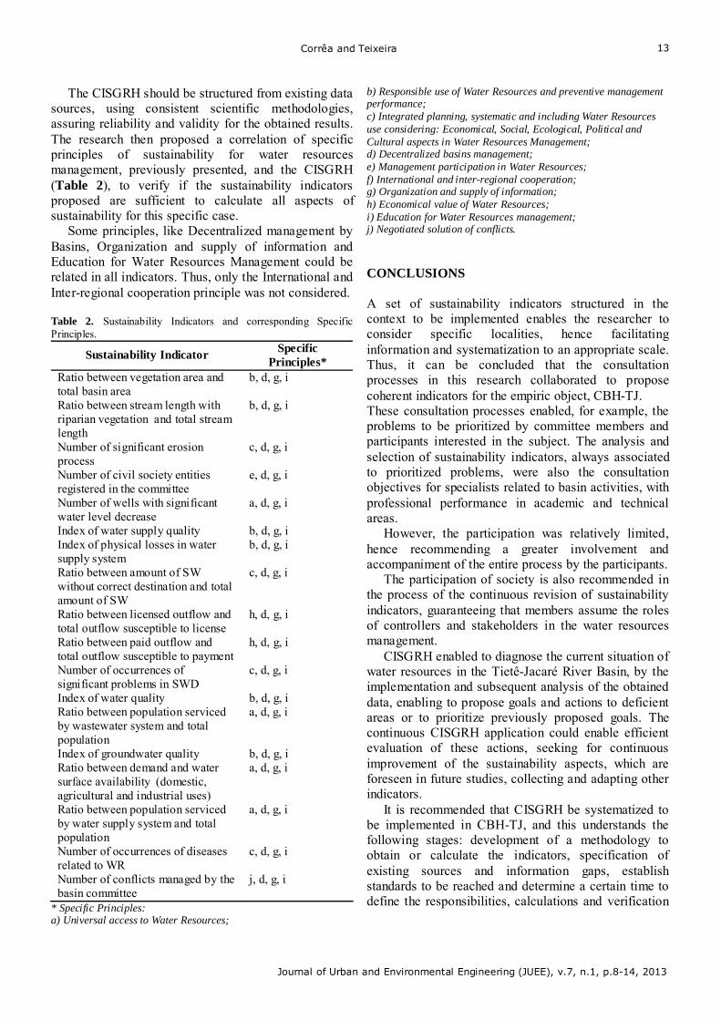
The CISGRH should be structured from existing data sources, using consistent scientific methodologies, assuring reliability and validity for the obtained results. The research then proposed a correlation of specific principles of sustainability for water resources management, previously presented, and the CISGRH (Table 2), to verify if the sustainability indicators proposed are sufficient to calculate all aspects of sustainability for this specific case.
Some principles, like Decentralized management by Basins, Organization and supply of information and Education for Water Resources Management could be related in all indicators. Thus, only the International and Inter-regional cooperation principle was not considered. Table 2. Sustainability Indicators and corresponding Specific Principles.
Sustainability Indicator Specific Principles*
Ratio between vegetation area and total basin area
b, d, g, i
Ratio between stream length with riparian vegetation and total stream length
b, d, g, i
Number of significant erosion process
c, d, g, i
Number of civil society entities registered in the committee
e, d, g, i
Number of wells with significant water level decrease
a, d, g, i
Index of water supply quality b, d, g, i Index of physical losses in water supply system
b, d, g, i
Ratio between amount of SW without correct destination and total amount of SW
c, d, g, i
Ratio between licensed outflow and total outflow susceptible to license
h, d, g, i
Ratio between paid outflow and total outflow susceptible to payment
h, d, g, i
Number of occurrences of significant problems in SWD
c, d, g, i
Index of water quality b, d, g, i Ratio between population serviced by wastewater system and total population
a, d, g, i
Index of groundwater quality b, d, g, i Ratio between demand and water surface availability (domestic, agricultural and industrial uses)
a, d, g, i
Ratio between population serviced by water supply system and total population
a, d, g, i
Number of occurrences of diseases related to WR
c, d, g, i
Number of conflicts managed by the basin committee
j, d, g, i
* Specific Principles: a) Universal access to Water Resources;
b) Responsible use of Water Resources and preventive management performance; c) Integrated planning, systematic and including Water Resources use considering: Economical, Social, Ecological, Political and Cultural aspects in Water Resources Management; d) Decentralized basins management; e) Management participation in Water Resources; f) International and inter-regional cooperation; g) Organization and supply of information; h) Economical value of Water Resources; i) Education for Water Resources management; j) Negotiated solution of conflicts.
CONCLUSIONS
A set of sustainability indicators structured in the context to be implemented enables the researcher to consider specific localities, hence facilitating information and systematization to an appropriate scale. Thus, it can be concluded that the consultation processes in this research collaborated to propose coherent indicators for the empiric object, CBH-TJ. These consultation processes enabled, for example, the problems to be prioritized by committee members and participants interested in the subject. The analysis and selection of sustainability indicators, always associated to prioritized problems, were also the consultation objectives for specialists related to basin activities, with professional performance in academic and technical areas.
However, the participation was relatively limited, hence recommending a greater involvement and accompaniment of the entire process by the participants.
The participation of society is also recommended in the process of the continuous revision of sustainability indicators, guaranteeing that members assume the roles of controllers and stakeholders in the water resources management.
CISGRH enabled to diagnose the current situation of water resources in the Tietê-Jacaré River Basin, by the implementation and subsequent analysis of the obtained data, enabling to propose goals and actions to deficient areas or to prioritize previously proposed goals. The continuous CISGRH application could enable efficient evaluation of these actions, seeking for continuous improvement of the sustainability aspects, which are foreseen in future studies, collecting and adapting other indicators.
It is recommended that CISGRH be systematized to be implemented in CBH-TJ, and this understands the following stages: development of a methodology to obtain or calculate the indicators, specification of existing sources and information gaps, establish standards to be reached and determine a certain time to define the responsibilities, calculations and verification
Corrêa and Teixeira
Journal of Urban and Environmental Engineering (JUEE), v.7, n.1, p.8-14, 2013
14
trends in relation to the previously established standards.
This procedure should obtain characterization conditions of the water resources and the tendency of these conditions with regards to the standards or goals established. This evaluation of tendencies for each indicator shows to stakeholders the gaps and priority areas that should be undertaken in the next stage.
It is recommended that sustainability indicators should be annually implemented for their progress and verification, as well as an effective evaluation of the actions proposed in the previous period. Spatial comparisons (other committees or inside the Tietê-Jacaré River Basin, and municipal districts) can also be accomplished.
REFERENCES
ANA – Agência Nacional das águas. Conjuntura dos recursos hídricos no Brasil 2009 / Agência Nacional de Águas. -- Brasília : ANA, 2009. 204 p. : Il. ISBN 978-85-89629-48-5.
ANZECC - Australian and New Zealand Environment Conservation Council. Core Environmental Indicators for Reporting on the State of the Environment. State of the Environment Reporting Task Force, 2000. Available in www.deh.gov.au/soe/publications/coreindicators.html.
Brasil. Presidência da República - Casa Civil - Subchefia para Assuntos Jurídicos. Lei nº. 9.433 de 08 de Janeiro de 1997 – Política Nacional de Recursos Hídricos. Available in <http://www.planalto.gov.br/CCIVIL/leis/L9433.htm>.
CETESB – Companhia de Tecnologia de Saneamento Ambiental. Relatório de Qualidade das Águas Interiores do Estado de São Paulo, (2004).
Comitês de Bacia Hidrográfica - CBH. Available in www.chb.gov.br, acess in 30/09/2010.
Corrêa, M. A. Teixeira, B. A. N. Desenvolvimento de Indicadores de Sustentabilidade para Gestão de Recursos Hídricos no âmbito de Comitê de Bacia Hidrográfica. In. 24°. Congresso Brasileiro de Engenharia Sanitária e Ambiental, 02 a 07 de setembro de 2007, Belo Horizonte.
Corrêa, M. A. Teixeira, B. A.N. Princípios Específicos de Sustentabilidade na Gestão de Recursos Hídricos por Bacia
Hidrográfica. In: III Encontro Associação Nacional de Pós-Graduação e Pesquisa em Ambiente e Sociedade – ANPPAS, 23 a 26 de Maio de 2006, Brasília.
EPA’s Draft Report on Environment: Technical Document, 2003. United States Environment Protection Agency. Office of Research and Development and the Office of Environment Information. www.epa.gov/indicators/. acesso 28/09/2005.
Fairweather, P.G. & Napier, G.M. Relatório de Indicadores Ambientais. Estado do Meio Ambiente SoE. Relatório Nacional do Estado do Meio Ambiente, Austrália. 1998. Available in <http://www.deh.gov.au/index.html> Acess in22/09/05.
Hezri, A.A. Sustainability indicator system and policy processes in Malaysia: a framework for utilisation and learning. Journal of Environmental Management 73 (2004) 357–371. Available in www.elsevier.com/locate/jenvman. Accessed in 20 de November 2010.
Ioris, A.A.R., Hunter, C., Walker, S. The development and application of water management sustainability indicators in Brazil and Scotland. Journal of Environmental Management 88 (2008) 1190–1201. Available in www.elsevier.com/locate/jenvman. Accessed in 20 de November de 2010.
MMA – Ministério do Meio Ambiente e ANA – Agência Nacional das Águas. GEO Brasil : recursos hídricos : componente da série de relatórios sobre o estado e perspectivas do meio ambiente no Brasil/Ministério do Meio Ambiente ; Agência Nacional de Águas ; Programa das Nações Unidas para o Meio Ambiente. Brasília : MMA; ANA, 2007. 264 p.: il. (GEO Brasil Série Temática : GEO Brasil Recursos Hídricos).
PERH - Plano Estadual de Recursos Hídricos, 2004-2007. Available in www.sigrh.sp.gov.br.
SÃO PAULO, Lei nº. 7.663 30 de Dezembro de 1991 – Política Nacional de Recursos Hídricos e Sistema Integrado de Gerenciamento de Recursos Hídricos.
Steinemann, A.C., Cavalcanti, L.F.N. (2006) Developing Multiple Indicators and Triggers for Drought Plans. In: Journal of Water Resources Planning and Management, 132(3), 26-36.
Van Bellen, H.M. Indicadores de Sustentabilidade: Uma análise Comparativa, 2002. Tese (Doutorado em Engenharia de Produção) – Curso de Pós-Graduação em Engenharia de Produção, Universidade Federal de Santa Catarina, 2002.
Xarxa, de Ciutats i Pobles cap a la Sostenibilitat. Sistema Municipal d’indicadors de sostenibilitat. Diputació Barcelona. Direção do projeto: Vicenç Sureda, 2000.
Zali, Azadeh and Salmani
Journal of Urban and Environmental Engineering (JUEE), v.7, n.1, p.15-23, 2013
15
Journal of Urban and Environmental Engineering, v.7, n.1, p.15-23
Journal of urban and Environmental Engineering
UEEJ ISSN 1982-3932 doi: 10.4090/juee.2013.v7n1.015023 ORG.EUE-JOURNAL.WWW
EVALUATION OF NEW TOWNS CONSTRUCTION IN THE AROUND OF TEHRAN MEGACITIY
Nader Zali1 , Seyed Reza Azadeh2, Taravat Ershadi Salmani3
1Assistant professor, Department of Urban Planning, University of Guilan, Iran 2 M.A Student, Department of Regional Planning, University of Guilan, Iran 3 M.A Student, Department of Regional Planning, University of Guilan, Iran
Received 09 May2012; received in revised form 1 June 2012; accepted 20 January 2013
Abstract: Rapid pace of urbanization which has affected third world countries is a by-product of the post-1945 period. In most developing countries like Iran, spatial population distribution is not balanced, leading to the deficiencies in services, hygiene, formation of slums, and etc. To balance those patterns in the country, different strategies have been applied, one of which is the construction of new cities. This study aims to examine the role of new cities in balancing spatial population distribution in Tehran province. For this purpose, first, the changes in the population of Iran and its urban mechanisms are studied; then, the performances of new towns in previous decades are examined. To analyze data and investigate the role of new cities, entropy coefficient model was used. The results showed that new towns of Tehran have not affected population overflow and deconcentration successfully; as a result, urban officials need to revise construction policies in those cities.
Keywords:
New towns; urban systems; population; decentralization; the coefficient of entropy; Iran.
© 2013 Journal of Urban and Environmental Engineering (JUEE). All rights reserved.
Correspondence to: Nader Zali. Tel.: +98 914 303 8588. E-mail: [email protected]
Zali, Azadeh and Salmani
Journal of Urban and Environmental Engineering (JUEE), v.7, n.1, p.15-23, 2013
16
INTRODUCTION New towns have been created during the history for many commonplace reasons, including: security, economic, demographic concerns and etc. But after Industrial Revolution, the trend of constructing new cities has been completely different from the past (Qrakhlu and Abedini, 2009). Since 1961, following land reformation plans, Islamic Republic of Iran and economic changes at global level, assembly industries were developed beside big cities, leading to rapid urbanization and the expansion of urban areas, creating many problems. Since 19611978, three major factors affecting rapid urbanization included migration of villagers to the cities, urban life’s blooming and fast population growth, and converting rural areas to urban places. The impact of population on the number of urban areas was also evident (Mashhdyzadeh Dehaghani, 2010).
Almost all statistics after the revolution have revealed a continuation of large-scale urbanization and an increasing tendency towards the concentration of urban population in a few big cities. The proportion of urban population to the total population of the country in 1976 reached 47%; while, it increased to 61% in 1996. Both the increase in the number of urban places and population increase in the cities have contributed to the process of urbanization (Fanni, 2006). Based on the statistics of 1957, published by Statistics Department of Iran, the number of the cities were 199. But, the statistics showed the number of 1,000 for the cities in Iran in 2006 (Barakpoor, Asadi, 2011). Regarding the mentioned points, growing urbanization, preventing from the growth of macropolitans and controlling natural growth rate of population, immigration needs to be monitored. If this fails, restoring the structures of the old cities is the best method for urban development. In the case this template does not control growing urban population, continuous development of the cities are considered in the places which are not faced with natural or artificial constraints. If these patterns do not work, other places should be regarded outside the metropolis for absorbing its population overflow. Since two first-mentioned patterns have not fulfilled desired goals, urban planners and policy-makers have resorted to decentralization of metropolises as a template to create new cities (Ebrahimzadeh and Negahban Marvee, 2006).
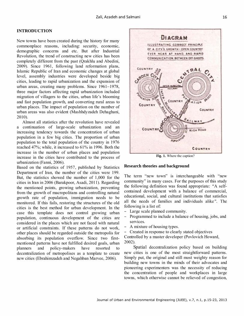
Fig. 1. Where the caption?
Research theories and background The term “new town” is interchangeable with “new community” in many cases. For the purposes of this study the following definition was found appropriate: “A self-contained development with a balance of commercial, educational, social, and cultural institutions that satisfies all the needs of families and individuals alike”. The following is a list of: − Large scale planned community. − Programmed to include a balance of housing, jobs, and
services. − A mixture of housing types. − Created in response to clearly stated objectives Controlled by a master developer (Povlovich Howard, 2002).
Spatial decentralization policy based on building new cities is one of the most straightforward patterns. Simply put, the original and still most weighty reason for building new towns in the minds of their advocates and pioneering experimenters was the necessity of reducing the concentration of people and workplaces in large towns, which otherwise cannot be relieved of congestion,
Zali, Azadeh and Salmani
Journal of Urban and Environmental Engineering (JUEE), v.7, n.1, p.15-23, 2013
17
disorder and squalor and rebuilt on a fully healthy, socially satisfactory, or efficient pattern.
In this context, the idea of creating new cities has been attributed to the English people. In 1898, the public in Britain was concerned about the influx of the people to the cities, leading to densely populated urban areas as a result of evacuating rural regions. In such conditions, “Ebenezer Howard”’s solution seemed less troublesome, without relying on any kind of sudden and radical changes or revolution. He was aware of the attractions of metropolises for villagers; so, he aimed to mix the advantages of urban life with the beauty of villages, creating town gardens. Developed in definite distances around a metropolis, such towns have a green belt around, connected via fast public transportation vehicles (Austrufsky, 2008). Until World War II, only two satellite cities of Latchverth and Welvynwere built with thirty-five thousand inhabitants. Great Britain had a population of ten millions; but, despite the predictions of Howard, two newly built towns around London could not prevent population influx to the capital city of Great Britain. After World War II, the construction model, suggested by Howard, revealed its positive results, benefiting from governmental support.
The pattern of new towns was adopted as a foundation for the organization and refinement of big cities. New towns can be planned and constructed in different models of satellite, independent, permanent, recreational and political-administrative types in Europe, America, Australia, Asia and Africa. Village garden, precinct garden, town garden, satellite town and New Towns represent different international models that have been planned and constructed on the basis of the garden cities’ conceptual framework, expanded globally (Ziari, 2006). In the third world countries, this theory was employed to enforce the strategy of decentralization, land use planning, establishing growth hub, regional development, transferring the office centers, spatial organization of small towns creating service hubs for rural areas, making centers for integration of village and reconstruction of demolished towns with various results. Totally, these towns were successful in providing housing for low-income households; but, their physical, social and economic structure was not consistent with local environment; therefore, they were considered luxurious and costly commodities that only caused the social imbalances. Even in some cases the slums were combined with the metropolises because they were designed according to local policies, overlooking the comprehensive national and regional strategies (Seyed Fatemi, 2010). In an article titled, «New town
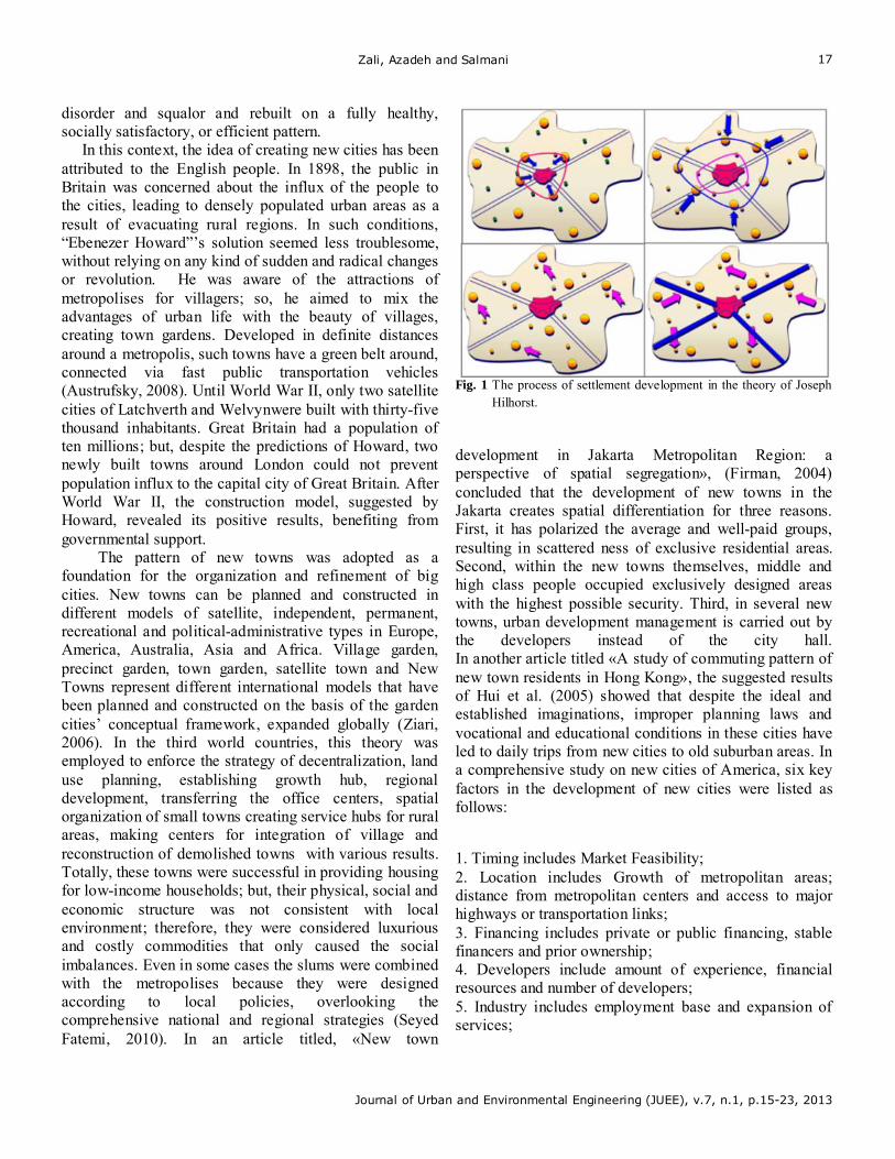
Fig. 1 The process of settlement development in the theory of Joseph
Hilhorst.
development in Jakarta Metropolitan Region: a perspective of spatial segregation», (Firman, 2004) concluded that the development of new towns in the Jakarta creates spatial differentiation for three reasons. First, it has polarized the average and well-paid groups, resulting in scattered ness of exclusive residential areas. Second, within the new towns themselves, middle and high class people occupied exclusively designed areas with the highest possible security. Third, in several new towns, urban development management is carried out by the developers instead of the city hall. In another article titled «A study of commuting pattern of new town residents in Hong Kong», the suggested results of Hui et al. (2005) showed that despite the ideal and established imaginations, improper planning laws and vocational and educational conditions in these cities have led to daily trips from new cities to old suburban areas. In a comprehensive study on new cities of America, six key factors in the development of new cities were listed as follows:
1. Timing includes Market Feasibility; 2. Location includes Growth of metropolitan areas; distance from metropolitan centers and access to major highways or transportation links; 3. Financing includes private or public financing, stable financers and prior ownership; 4. Developers include amount of experience, financial resources and number of developers; 5. Industry includes employment base and expansion of services;

Zali, Azadeh and Salmani
Journal of Urban and Environmental Engineering (JUEE), v.7, n.1, p.15-23, 2013
18
Table 1. Population changes of Iran between 19572007
Year Total population of country
Rate of population growth
Population of urban areas
Population of rural areas
Urbanisatipon percent
Number of cities
1957 18 954 704 6 002 621 12 952 083 31.4 200 1967 25 788 722 3.13 9 795 810 15 992 912 38 272 1977 33 708 744 2.71 15 854 680 17 854 064 47 373 1987 49 445 010 3.91 26 844 561 22 600 449 54.3 496 1997 60 055 488 1.96 36 817 789 23 237 699 61.3 612 2007 70 495 782 1.62 48 259 964 22 235 818 68.6 1012
6. Government includes permitting process, relationship with local region and political support. (Pavlovich Howard, 2002).
In recent years, because of the fast growth of big cities in developing countries and the existence of empty new towns, some researchers have proposed that development plans should be prepared based on the dynamism of small and intermediate towns (Shokooi, 2006).
One of the most important theories in the field of spatial development belongs to Joseph Hylhorst. Due to the importance of spatial development strategies to eliminate interregional, intraregional, and sectorial duplications, proportional to hierarchy of settlements and residents, Hylhorst suggests four different strategies (quoted by Ardeshiri, 1993): 1. concentrate consolidation; 2. dispersed consolidation; 3. concentrate expansion; 4. dispersed expansion.
Hylhorst posits two main suppositions in those four strategies: expansion and consolidation. Reinforcing self-concentration (i.e. convergent forces), the former is used for the provinces or regions which are at the elementary phases of development, ranked among deprived or poor provinces (Fig. 1a). While, the latter focuses on around center reinforcements (i.e. divergent forces) (Fig. 1b).
Expansion stage has two different strategies based on area location. For properly distributed and developed areas convergent concentration is offered (Fig. 1c). Investment in a new regional center or second-grade regional centers is a basic suggestion of this theory. The last phase of development is using divergent concentration (Fig. 1d). This strategy suits for the provinces with balanced spatial structure, aiming to transferdevelopment across the whole region and its nearby (Hilhorst, 1971). Materials and Methods
This study used library method to gather data. Exerting extant documents, the performances of the new towns were studied. Via statistics, population changes and urban mechanisms were investigated.
Entropy coefficient model was used for data analysis. This standard model is a measure for examining the distribution of urban population and the number of the cities in a region. This model can be used to examine the balance of population and city number in urban, provincial, regional, and national levels. The overall structure of the model is as follows:
G = (ΣPi LnPi)/LnKG: Coefficient of Entropy K: Number of Floors Pi: Abundance LnPi: Frequency logarithm of Nepery
In this model, if the entropy tends to zero, there will be higher concentration or imbalance in population distribution in the cities; while, moving toward 1 or above reveals a more balance distribution in the region (Hekmatniaand & Mousavi, 2006).
Changes in population and urbanization growth Since 18691957, urban mechanisms in Iran were homogenous and balanced in a way that no city had superiority to the others. Every city served and connected its surrounding villages with convergent and consistent concentration (Ziari, 2009). Based on the first official statistics of 1957, the population of Iran was estimated to be18.9 million people, raisnig to 25.7 million people in 1967. Then, Iran had a population growth of 3.1%.
During 19671977, population growth rate was 2.7%, reaching 3.9% by the next decade. In 1966, Iran faced with a declining growth rate of the population with the estimated population of 60 million. The next decade witnessed a declining trend again. In 2006, Iran had a population of 70.4 million. Thus, Iran had a decreasing population growth rate in two last decades.
The reasons of the such decline in the annual population growth rate are attributed partially to the government’s family planning efforts since 1989 and the dismal economic conditions and general decline in living
Zali, Azadeh and Salmani
Journal of Urban and Environmental Engineering (JUEE), v.7, n.1, p.15-23, 2013
19
standards for the average Iranian households (Ziari, 2006). Population and housing studies in 1957 to 2006 indicate a population increase of about 52 million people in Iran. Like many developing countries, urbanization in Iran has a growing trend. According to the Population and Housing statistics in 1957, the urban population of Iran with 200 urban areas was approximately 6 million people, raising to 15.8 million within twenty years to the Islamic Revolution. After the Islamic Revolution of 1957 until 2006, the urban population of the country increased to 48.2 million. In a fifty-year period from 19572006, urban areas reached 1012 areas. The statistics suggest that the urbanization coefficient increased from 31.7% in 1957 to 68.5% in 2006.
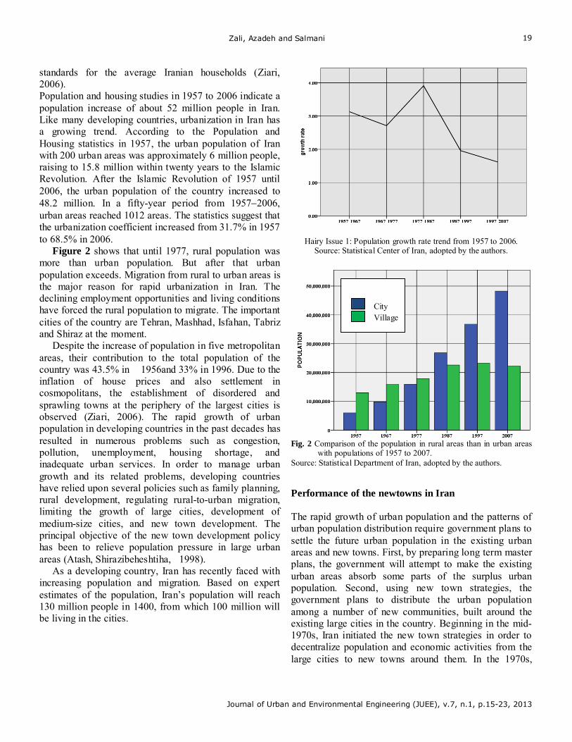
Figure 2 shows that until 1977, rural population was more than urban population. But after that urban population exceeds. Migration from rural to urban areas is the major reason for rapid urbanization in Iran. The declining employment opportunities and living conditions have forced the rural population to migrate. The important cities of the country are Tehran, Mashhad, Isfahan, Tabriz and Shiraz at the moment.
Despite the increase of population in five metropolitan areas, their contribution to the total population of the country was 43.5% in 1956 and 33% in 1996. Due to the inflation of house prices and also settlement in cosmopolitans, the establishment of disordered and sprawling towns at the periphery of the largest cities is observed (Ziari, 2006). The rapid growth of urban population in developing countries in the past decades has resulted in numerous problems such as congestion, pollution, unemployment, housing shortage, and inadequate urban services. In order to manage urban growth and its related problems, developing countries have relied upon several policies such as family planning, rural development, regulating rural-to-urban migration, limiting the growth of large cities, development of medium-size cities, and new town development. The principal objective of the new town development policy has been to relieve population pressure in large urban areas (Atash, Shirazibeheshtiha, 1998).
As a developing country, Iran has recently faced with increasing population and migration. Based on expert estimates of the population, Iran’s population will reach 130 million people in 1400, from which 100 million will be living in the cities.
Hairy Issue 1: Population growth rate trend from 1957 to 2006.
Source: Statistical Center of Iran, adopted by the authors.
Fig. 2 Comparison of the population in rural areas than in urban areas
with populations of 1957 to 2007. Source: Statistical Department of Iran, adopted by the authors.
Performance of the newtowns in Iran
The rapid growth of urban population and the patterns of urban population distribution require government plans to settle the future urban population in the existing urban areas and new towns. First, by preparing long term master plans, the government will attempt to make the existing urban areas absorb some parts of the surplus urban population. Second, using new town strategies, the government plans to distribute the urban population among a number of new communities, built around the existing large cities in the country. Beginning in the mid-1970s, Iran initiated the new town strategies in order to decentralize population and economic activities from the large cities to new towns around them. In the 1970s,
City Village

Zali, Azadeh and Salmani
Journal of Urban and Environmental Engineering (JUEE), v.7, n.1, p.15-23, 2013
20
several new towns were proposed and developed, planned as residential communities or industrial towns around a few large cities such as Tehran and Esfahan (Atash, Shirazibeheshtiha, 1998).
The urbanization system of Iran can be evaluated in four periods: 1- In the distance between the two world wars, new
towns of Iran were planned without specific strategy evolved around a core rural area. For example, Zahedan and Noshahr which are regarded thriving at the moment.
2- During World War II until the mid-1960s, Iranian towns were developed without specific strategy, evolving around an urban core for the development of oil and other industry.
3- From mid-1960 to 1969, new towns were formed with the aim of exploiting natural resources without any primary nucleaus, regional development, land use, or housing.
4- Aiming to spatially organize and revise metroplitans and balance their economic growth, 28 satellite towns were developed without a primary core to settle 6 million people until 2016, absorbing population overflow. The plan of Urban Development after Islamic revolution was first legislated by the Committee of Governmental Employees Welfare in Housing Ministry which led to Act No. 108328, as the main key in decision-makings for this plan. After legislation of this this act, 24 other towns were built and 11 more towns are being constructed (Ziari, 2009).
It is important to point out that the urban population of the country was over 48 million persons in 2006, while only 7.9% (3.8 millions) of this population were settled in new towns. On the other hand, the decision was to settle 1.6% of this population in these towns by the end of the fourth development program; thus, calculating the present population of these towns, only 0.7% of the urban population of the country could be settled in new towns. The key question is that can any other strategy be a proper alternative in order to attract and settle this 0.7% of urban population, excluding the construction of new towns?
The most important problems in these towns are as follow: • Dependence on one economic activity and the single
base of employment; • Exclusive ownership of the houses and lands of the city
by the company; • Uniform organizational house pattern;
Fig. 3 Tehran’s position in the country’s political divisions and urban centers of the province. • Dependence on the services of the company; • Separation of the town from the network of the cities
and villages in the area; • Lack of development; • Social and cultural conflicts; • Heavy maintenance costs; • Dormitory nature of the towns (Ziari and Qrakhlu,
2009).
STUDY SCOPE As one of the thirty provinces of Iran, Tehran has 15 cities, 37 districts and 83 villages. Urban areas of the province consist of 56 towns and 1201 villages with inhabitants. Tehran Province has an area of about 18 814 square kilometers, located in 34 degrees and 52 minutes to 36 degrees and 19 minutes of north latitude and between 50 degrees and 10 minutes to 53 degrees and 10 minutes east longitude from Greenwich Hour Circle. Figure 3 shows the location ofTehran Province and its subdivisions with their centers. Population changes and entropy coefficient analysis of urbanization mechanisms in Tehran Development and population density are the main features of the urbanization mechanisms in Iran. Tehran has maintained its superiority in economic and social aspects of this system. As a metropolitan area, Tehranhas dominates in political, organizational, and economic aspects over other cities. Then, like any other third world country, Iran has a first urban template (Jajromi and Gheibi, 2011).
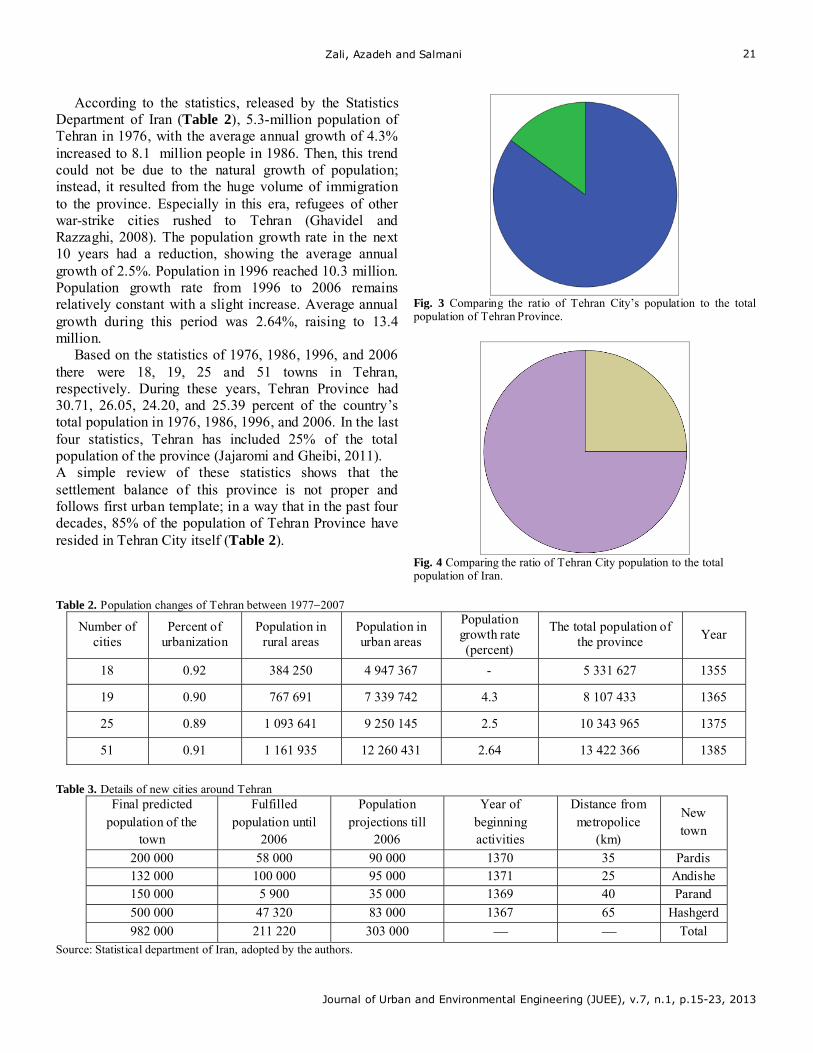
Zali, Azadeh and Salmani
Journal of Urban and Environmental Engineering (JUEE), v.7, n.1, p.15-23, 2013
21
According to the statistics, released by the Statistics Department of Iran (Table 2), 5.3-million population of Tehran in 1976, with the average annual growth of 4.3% increased to 8.1 million people in 1986. Then, this trend could not be due to the natural growth of population; instead, it resulted from the huge volume of immigration to the province. Especially in this era, refugees of other war-strike cities rushed to Tehran (Ghavidel and Razzaghi, 2008). The population growth rate in the next 10 years had a reduction, showing the average annual growth of 2.5%. Population in 1996 reached 10.3 million. Population growth rate from 1996 to 2006 remains relatively constant with a slight increase. Average annual growth during this period was 2.64%, raising to 13.4 million.
Based on the statistics of 1976, 1986, 1996, and 2006 there were 18, 19, 25 and 51 towns in Tehran, respectively. During these years, Tehran Province had 30.71, 26.05, 24.20, and 25.39 percent of the country’s total population in 1976, 1986, 1996, and 2006. In the last four statistics, Tehran has included 25% of the total population of the province (Jajaromi and Gheibi, 2011). A simple review of these statistics shows that the settlement balance of this province is not proper and follows first urban template; in a way that in the past four decades, 85% of the population of Tehran Province have resided in Tehran City itself (Table 2).
Fig. 3 Comparing the ratio of Tehran City’s population to the total population of Tehran Province.
Fig. 4 Comparing the ratio of Tehran City population to the total population of Iran.
Table 2. Population changes of Tehran between 19772007
Year The total population of
the province
Population growth rate (percent)
Population in urban areas
Population in rural areas
Percent of urbanization
Number of cities
1355 5 331 627 - 4 947 367 384 250 0.92 18
1365 8 107 433 4.3 7 339 742 767 691 0.90 19
1375 10 343 965 2.5 9 250 145 1 093 641 0.89 25
1385 13 422 366 2.64 12 260 431 1 161 935 0.91 51
Table 3. Details of new cities around Tehran
New town
Distance from metropolice
(km)
Year of beginning activities
Population projections till
2006
Fulfilled population until
2006
Final predicted population of the
town
Pardis 35 1370 90 000 58 000 200 000 Andishe 25 1371 95 000 100 000 132 000 Parand 40 1369 35 000 5 900 150 000
Hashgerd 65 1367 83 000 47 320 500 000
Total 303 000 211 220 982 000 Source: Statistical department of Iran, adopted by the authors.
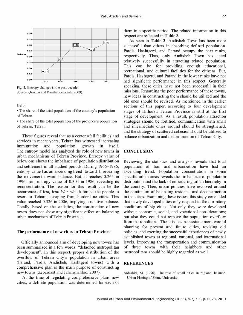
Zali, Azadeh and Salmani
Journal of Urban and Environmental Engineering (JUEE), v.7, n.1, p.15-23, 2013
22
Fig. 5. Entropy changes in the past decade. Source: Qrakhlu and Panahandehkhah (2009).
Help: • The share of the total population of the country’s population of Tehran • The share of the total population of the province’s population of Tehran, Tehran
These figures reveal that as a center ofall facilities and services in recent years, Tehran has witnessed increasing immigration and population growth in itself. The entropy model has analyzed the role of new towns in urban mechanisms of Tehran Province. Entropy value of below one shows the imbalance of population distribution and settlement in all studied periods. During 19661986, entropy value has an ascending trend toward 1, revealing the movement toward balance. But, it reaches 0.265 in 1996 from entropy value of 0.304 in 1986, revealing its reconcentration. The reason for this result can be the occurrence of Iraq-Iran War which forced the people to resort to Tehran, escaping from border-line cities. This value reached 0.326 in 2006, implying a relative balance. Totally, based on the statistics, the construction of new towns does not show any significant effect on balancing urban mechanism of Tehran Province.
The performance of new cities in Tehran Province
Officially announced aim of developing new towns has been summarized in a few words: “detached metropolitan development”. In this respect, proper distribution of the overflow of Tehran City’s population in urban areas (Parand, Pardis, Andisheh, Hashtgerd towns) with a comprehensive plan is the main purpose of constructing new towns (Zebardast and Jahanshahloo, 2007).
At the time of legislating comprehensive plans new cities, a definite population was determined for each of
them in a specific period. The related information in this respect are reflected in Table 3.
As seen in Table 3, Andisheh Town has been more successful than others in absorbing defined population. Pardis, Hashtgerd, and Parand occupy the next ranks, respectively. Thus, only Andisheh Town has acted relatively successfully in attracting related population. This can be for providing enough educational, recreational, and cultural facilities for the citizens. But, Pardis, Hashtgerd, and Parand in the lower ranks have not had significant performance in this respect. Generally speaking, these cities have not been successful in their missions. Regarding the poor performance of these towns, new ideas in constructing them should be utilized and the old ones should be revised. As mentioned in the earlier sections of this paper, according to four development stages of Hilhorst, Tehran Province is still at the first stage of development. As a result, population attraction strategies should be fortified, communication with small and intermediate cities around should be strengthened, and the strategy of scattered cohesion should be utilized to balance urbanization and deconstruction of Tehran City.
CONCLUSION Reviewing the statistics and analysis reveals that total population of Iran and urbanization have had an ascending trend. Population concentration in some specific urban areas reveals the imbalance of population distribution and the lack of considering urban hierarchy in the country. Then, urban policies have revolved around the continuum of balancing residents and deconstruction in the cities. Examining these issues, this study concluded that newly developed cities only respond to the dormitory conditions of big cities. Not only they were developed without economic, social, and vocational considerations; but also they could not remove the population overflow from metropolitans. These issues necessitate more careful planning for present and future cities, revising old policies, and exerting the successful experiences of newly established towns at regional, national, and international levels. Improving the transportation and communication of these towns with their neighbors and other metropolitans should be highly regarded as well. REFERENCES Ardeshiri, M. (1990). The role of small cities in regional balance.
Urban Planing of Shiraz University.

Zali, Azadeh and Salmani
Journal of Urban and Environmental Engineering (JUEE), v.7, n.1, p.15-23, 2013
23
Austufsky, V.(2008). Contemprory city constructionn from the begining until Athen Charter. Translated by Etezadi, L. University Publication.
Atash, F., Shirazibeheshtiha, Y. S. (1998). New towns and their practical challenges: The experience of Poolad Shahr in Iran. HABITATITNL., Vol. 22, No. 1, 1-13.
Barakpoor, N., Asadi, I. (2011). Urban management and organization. Art University Publication.
Ebrahimzadeh, I., Negahbanmarvi, M. (2006). Analysis of urbanization and the role of new cities in Iran. Geographic Research Quarterly, No. 75, summer.
Fanni, Z. (2006). Cities and urbanization in Iran after the Islamic revolution. Cities, Vol. 23, No. 6, 407–411.
Firman, T. (2004). New town development in Jakarta’s metropolitanregion: A perspective of spatial segregation, Habitat International, 28.
Fatemi, S.M., Hosainzadeh-Dalir,K. (2010). Analysis of Sahand New Town role in spatial order of Tabriz urban region. Urban - Regional Studies and Research Journal, 2(6), Autumn.
Gharakhloo, M., Abedini, A. (2009). Challenges of new cities and their success in Iran, case study of Sahand Town, Human Sciences Quarterly, 3(1).
Gharakhloo, M., Panahandehkhah, M. (2008). Evaluating the performance of new cities in attracting surplus population of Tehran, case study of new towns around Tehran. Human Geography Researches, No. 67.
Ghavidel, S., Razzaghi, H., and Alipoor, Kh.(2008). Examining the reasons for migration to Tehran metropolitan, focusing on Firoozkooh Town, Economic Quarterly, No. 1.
Hekmatnia,H., Mosavi, N.(2006).Model applications in geography using urban planning. New Sciences Publication.
Hui, E C.M., Lam Manfred, C.M. 2005. A study of commuting patterns of new towns’ residents in Hong Kong, Habitat International ,Vol. 29, Hilhorst, J.G.M. (1971). Regional planning: A systematic approach. Rotterdam University Press.
Jajromi,K., Gheibi, M. (2011). Analyzing the mechanisms of Tehran from 1967-2006. Scientific Quarterly of New Attitudes in Human Geography, 3(3).
Mashhadizadeh, Dehagani, N. (2010). An analysis of urban planning features in Iran, Science and Industry University Publication.
Pavlovich Howard, Z. (2002). New Towns: An overview of 30 American new communities. CRP 410: Community Planning Laboratory.
Statistics Departmnet of Iran. Available at http://www.sci.org.ir. Ziari, K. (2006). The planning and functioning of new towns in Iran.
Towns. Vol. 23, No. 6, 412-21. Ziari, K., Gharakhlou, M. A. (2009). Study of Iranian new towns
during pre- and post-revolution. Int. J. Environ. Res., 3(1):143-154, Winter.
Ziari, K. (2009). New cities plans. Samt Publication. Shokooi,H. (2006). New Attitudes In Urban Geography, Vol.1, Samt
Publication. Zebardast, S., Jahanshahloo, L. (2007). Investigating the performance
of new town of Hashtgerd in absorbing population overflow. Geography and Development, No. 10.

Roy, Mondal, Das and Das
Journal of Urban and Environmental Engineering (JUEE), v.7, n.1, p.24-29 2013
24
Journal of Urban and Environmental Engineering, v.7, n.1, p.24-29
Journal of Urban and Environmental Engineering
UEEJ ISSN 1982-3932
doi: 10.4090/juee.2013.v7n1.024029 www.journal-uee.org
ARSENIC CONTAMINATION IN GROUNDWATER: A STATISTICAL MODELING
Palas Roy, Naba Kumar Mondal, Biswajit Das, and Kousik Das
Department of Environmental Science, The University of Burdwan, Burdwan, India, WB
Received 27 April 2012; received in revised form 27 January 2013; accepted 30 January 2012
Abstract: High arsenic in natural groundwater in most of the tubewells of the Purbasthali- Block
II area of Burdwan district (W.B, India) has recently been focused as a serious environmental concern. This paper is intending to illustrate the statistical modeling of the arsenic contaminated groundwater to identify the interrelation of that arsenic contain with other participating groundwater parameters so that the arsenic contamination level can easily be predicted by analyzing only such parameters. Multivariate data analysis was done with the collected groundwater samples from the 132 tubewells of this contaminated region shows that three variable parameters are significantly related with the arsenic. Based on these relationships, a multiple linear regression model has been developed that estimated the arsenic contamination by measuring such three predictor parameters of the groundwater variables in the contaminated aquifer. This model could also be a suggestive tool while designing the arsenic removal scheme for any affected groundwater.
Keywords:
Arsenic; groundwater; statistical modeling; multivariate analysis.
© 2013 Journal of Urban and Environmental Engineering (JUEE). All rights reserved.
Correspondence to: Naba K. Mondal, Mobile.:+919434545694. E-mail: [email protected]
Roy, Mondal, Das and Das
Journal of Urban and Environmental Engineering (JUEE), v.7, n.1, p.24-29 2013
25
INTRODUCTION
Arsenic contamination of groundwater is a major public health concern in West Bengal and elsewhere (Rahman et al., 2005). Millions of people have been exposed arsenic through drinking water that comes majorly from ground water (Duker et al., 2005). Chronic toxicity of arsenic in human from arsenic contaminated drinking water occurs in 3417 villages over 111 blocks, primarily within 12 districts of this state (Mondal et al., 2011), affecting more than 1.5 million of people (De, 2008) of which 25% are suffering arsenical skin lesions. The maximum permissible level of arsenic in drinking water recommended by World Health Organization (WHO) 0.01 mg/liter and in West Bengal it has been adjusted to 0.05 mg/liter by the local authorities. Drinking water arsenic concentration in West Bengal ranged from 0.05 to 3.5 mg/liter are reported on those affected zones which are in the vicinity of river Ganga (Das, 2008) and confined within the member delta zone of the upper delta plain. It has been reported by Nag et al. (1996) that water of the intermediate (second) aquifer is polluted with arsenic; though in some areas deep (third) aquifer has been detected where there is no clay partition between the second and third aquifer.
Drinking water arsenic contamination is originated from the natural release of arsenic through aquifer and sedimentary rocks (Zandsalimi et al., 2011). The element is fundamental constitute of sulphide minerals of which pyrite like, arseniopyrite, FeAsS, (McGurie et al., 2001) is the most abundant. Arsenopyrite is highly insoluble in water but due to anthropogenic activities (Aktar & Ali, 2011) it dissolved via oxygenation with formation of soluble arsenate and arsenite. In West Bengal arsenic species in contaminated drinking water were found to be arsenate and arsenite in 1:1 ratio (De, 2008). Pyrite oxidation has been proven to be the most acceptable hypothesis to explain the occurrence of arsenic in ground level water (Fazal et al., 2001). Therefore, the occurrence of arsenic might be coupled with the presence of iron (Fe) in water. Analysis of such groundwater in arsenic bearing zones also indicated the presence of high contain of Fe (Nag et al., 1996). This would strengthen the correlation between arsenic and iron concentration of ground water more rational. Though several authors also reported an interrelation of groundwater arsenic concentration with Static water level (SWL) (Welch & Stollenwerk, 2003), Depth (Chakraborti et al., 2009), pH (Saxena et al., 2004) and Age (time) of the wells (Fazal et al., 2001) at a regional level.
Now a day, interest has been also grown in determining of antimony (Sb) in groundwater due to its similar chemio-toxicological properties (Gibel, 1997) with arsenic though Sb-induced toxicity is more violent
vomiting in accompanied with watery diarrhea and sever weakness (Das, 2008). Antimony occurs with sulfur bed as same as arsenic, generally in the form of antimonite (Sb2S3) (Siepak et al., 2004). The unstable Sb2S3 decomposed via atmospheric oxygenation with formation of soluble oxide minerals of antimony and migrated into groundwater (Ashley et al., 2003) as a similar way of arsenic. In comparison to other toxic metals very little information exists on antimony in environmental sample, probably as a result of its low groundwater concentration, normally range from 0.1 to 0.2 µg/liter (WHO).
Then, for our present interest, a regional level groundwater quality survey in the Purbasthali- Block II area of Burdwan district (W.B, India) was conducted, which is identified as an arsenic polluted area (Biswas, 2010; Mondal et al., 2011). Groundwater samples from different tube wells were collected from 33 affected villages of the study area (Mondal et al., 2011). The purpose of this article is also to ascertain the possible interrelation of Arsenic, Sb, Fe, pH, Depth, SWL and Age of the tubewells through statistical modeling on the basic on such water samples. MATERIALS AND METHODS Water Sampling One hundred and thirty-two tubewell water samples were collected from different locations of Purbasthali Block-II in Burdwan district, West Bengal, India, in the month of September to October, 2011. The samples were collected in pre-cleaned sterilized polyethylene bottles of one liter capacity following standard protocol. To avoid any contamination at the source, the samples were taken by holding the bottles at the bottom and drawn directly from the tubewell after water was allow running at least fifteen (15) minutes (Karthikeyan et al., 2010). The water samples were immediately refrigerated after collection and brought to the laboratory with extreme care and preserved for further analysis. Reagents and standards Chemical of analytical grade were procured from M/S, Merck India Ltd; and used through the study without further purification. To prepare all reagents and standards, double distilled water was used. All glassware was cleaned by being soaked in 15% HNO3 and rinsed with double distilled water. Each sample was analyzed three times and the results were found reproducible within ± 3 error limit.
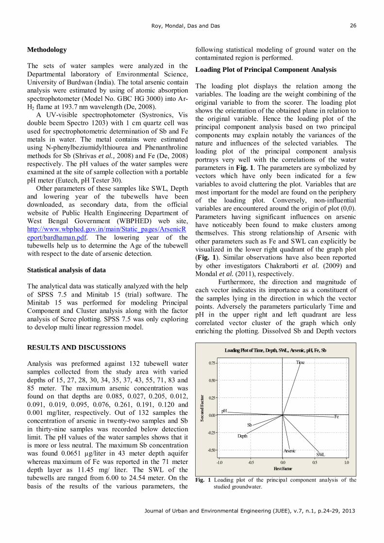
Roy, Mondal, Das and Das
Journal of Urban and Environmental Engineering (JUEE), v.7, n.1, p.24-29, 2013
26
Methodology The sets of water samples were analyzed in the Departmental laboratory of Environmental Science, University of Burdwan (India). The total arsenic contain analysis were estimated by using of atomic absorption spectrophotometer (Model No. GBC HG 3000) into Ar-H2 flame at 193.7 nm wavelength (De, 2008).
A UV-visible spectrophotometer (Systronics, Vis double beem Spectro 1203) with 1 cm quartz cell was used for spectrophotometric determination of Sb and Fe metals in water. The metal contains were estimated using N-phenylbeziumidylthiourea and Phenanthroline methods for Sb (Shrivas et al., 2008) and Fe (De, 2008) respectively. The pH values of the water samples were examined at the site of sample collection with a portable pH meter (Eutech, pH Tester 30).
Other parameters of these samples like SWL, Depth and lowering year of the tubewells have been downloaded, as secondary data, from the official website of Public Health Engineering Department of West Bengal Government (WBPHED) web site, http://www.wbphed.gov.in/main/Static_pages/ArsenicReport/bardhaman.pdf. The lowering year of the tubewells help us to determine the Age of the tubewell with respect to the date of arsenic detection.
Statistical analysis of data The analytical data was statically analyzed with the help of SPSS 7.5 and Minitab 15 (trial) software. The Minitab 15 was performed for modeling Principal Component and Cluster analysis along with the factor analysis of Scree plotting. SPSS 7.5 was only exploring to develop multi linear regression model.
RESULTS AND DISCUSSIONS Analysis was preformed against 132 tubewell water samples collected from the study area with varied depths of 15, 27, 28, 30, 34, 35, 37, 43, 55, 71, 83 and 85 meter. The maximum arsenic concentration was found on that depths are 0.085, 0.027, 0.205, 0.012, 0.091, 0.019, 0.095, 0.076, 0.261, 0.191, 0.120 and 0.001 mg/liter, respectively. Out of 132 samples the concentration of arsenic in twenty-two samples and Sb in thirty-nine samples was recorded below detection limit. The pH values of the water samples shows that it is more or less neutral. The maximum Sb concentration was found 0.0651 µg/liter in 43 meter depth aquifer whereas maximum of Fe was reported in the 71 meter depth layer as 11.45 mg/ liter. The SWL of the tubewells are ranged from 6.00 to 24.54 meter. On the basis of the results of the various parameters, the
following statistical modeling of ground water on the contaminated region is performed.
Loading Plot of Principal Component Analysis The loading plot displays the relation among the variables. The loading are the weight combining of the original variable to from the scorer. The loading plot shows the orientation of the obtained plane in relation to the original variable. Hence the loading plot of the principal component analysis based on two principal components may explain notably the variances of the nature and influences of the selected variables. The loading plot of the principal component analysis portrays very well with the correlations of the water parameters in Fig. 1. The parameters are symbolized by vectors which have only been indicated for a few variables to avoid cluttering the plot. Variables that are most important for the model are found on the periphery of the loading plot. Conversely, non-influential variables are encountered around the origin of plot (0,0). Parameters having significant influences on arsenic have noticeably been found to make clusters among themselves. This strong relationship of Arsenic with other parameters such as Fe and SWL can explicitly be visualized in the lower right quadrant of the graph plot (Fig. 1). Similar observations have also been reported by other investigators Chakraborti et al. (2009) and Mondal et al. (2011), respectively.
Furthermore, the direction and magnitude of each vector indicates its importance as a constituent of the samples lying in the direction in which the vector points. Adversely the parameters particularly Time and pH in the upper right and left quadrant are less correlated vector cluster of the graph which only enriching the plotting. Dissolved Sb and Depth vectors
1.00.50.0-0.5-1.0
0.75
0.50
0.25
0.00
-0.25
-0.50
First Factor
Sec
ond
Fact
or
Sb
FepH
ArsenicSWL
Depth
Time
Loading Plot of Time, Depth, SWL, Arsenic, pH, Fe, Sb
Fig. 1 Loading plot of the principal component analysis of the
studied groundwater.
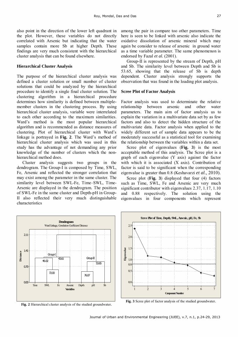
Roy, Mondal, Das and Das
Journal of Urban and Environmental Engineering (JUEE), v.7, n.1, p.24-29, 2013
27
also point in the direction of the lower left quadrant in the plot. However, these variables do not directly correlated with Arsenic but indicating that the water samples contain more Sb at higher Depth. These findings are very much consistent with the hierarchical cluster analysis that can be found elsewhere. Hierarchical Cluster Analysis The purpose of the hierarchical cluster analysis was defined a cluster solution or small number of cluster solutions that could be analyzed by the hierarchical procedure to identify a single final cluster solution. The clustering algorithm in a hierarchical procedure determines how similarity is defined between multiple-member clusters in the clustering process. By using hierarchical cluster analysis, variable were interrelated to each other according to the maximum similarities. Ward’s method is the most popular hierarchical algorithm and is recommended as distance measures of clustering. Plot of hierarchical cluster with Ward’s linkage is portrayed in Fig. 2. The Ward’s method of hierarchical cluster analysis which was used in this study has the advantage of not demanding any prior knowledge of the number of clusters which the non- hierarchical method does.
Cluster analysis suggests two groups in the dendrogram. The Group-I is composed by Time, SWL, Fe, Arsenic and reflected the stronger correlation that may exist among the parameter in the same cluster. The similarity level between SWL-Fe, Time–SWL, Time-Arsenic are displayed in the dendrogram. The position of SWL-Fe in the same cluster and Depth-pH in Group-II also reflected their very much distinguishable characteristics
SbpHDepthArsenicFeSWLTime
2.11
1.41
0.70
0.00
Variables
Dis
tanc
e
DendrogramWard Linkage, Correlation Coefficient Distance
Group-IGroup-II
46.02
72.00
43.61
76.07
53.65
Fig. 2 Hierarchical cluster analysis of the studied groundwater.
among the pair in compare too other parameters. Time here is seen to be linked with arsenic also indicate the oxidative dissolution of arsenic mineral which may again be consider to release of arsenic in ground water as a time variable parameter. The same phenomenon is endorsed by Fazal et al. (2001).
Group-II is represented by the stream of Depth, pH and Sb. The similarity level between Depth and Sb is 53.65, showing that the release of Sb is depth dependent. Cluster analysis strongly supports the observation that was found in the loading plot analysis. Scree Plot of Factor Analysis Factor analysis was used to determinate the relative relationship between arsenic and other water parameters. The main aim of factor analysis us to explain the variation in a multivariate data set by as few factors and also to detect the hidden structure of the multivariate data. Factor analysis when applied to the widely different set of sample data appears to be the moderately successful as a statistical tool for examining the relationship between the variables within a data set.
Scree plot of eigenvalues (Fig. 3) is the most acceptable method of this analysis. The Scree plot is a graph of each eigenvalue (Y axis) against the factor with which it is associated (X axis). Contribution of factor is said to be significant when the corresponding eigenvalue is greater than 0.8 (Keshavarzi et al., 2010).
Scree plot (Fig. 3) displayed that four (4) factors such as Time, SWL, Fe and Arsenic are very much significant contributor with eigenvalues 2.37, 1.17, 1.10 and 0.88 respectively. The solution using the eigenvalues in four components which represent
7654321
2.5
2.0
1.5
1.0
0.8
0.5
0.0
Component Number
Eig
enva
lue
Scree Plot of Time, Depth, SWL, Arsenic, pH, Fe, Sb
Fig. 3 Scree plot of factor analysis of the studied groundwater.
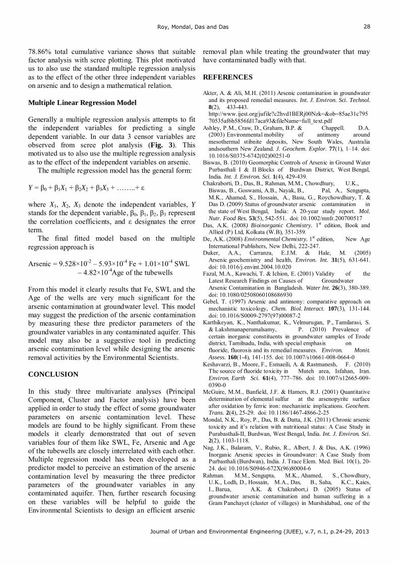
Roy, Mondal, Das and Das
Journal of Urban and Environmental Engineering (JUEE), v.7, n.1, p.24-29, 2013
28
78.86% total cumulative variance shows that suitable factor analysis with scree plotting. This plot motivated us to also use the standard multiple regression analysis as to the effect of the other three independent variables on arsenic and to design a mathematical relation. Multiple Linear Regression Model Generally a multiple regression analysis attempts to fit the independent variables for predicting a single dependent variable. In our data 3 censor variables are observed from scree plot analysis (Fig. 3). This motivated us to also use the multiple regression analysis as to the effect of the independent variables on arsenic.
The multiple regression model has the general form: Y = β0 + β1X1 + β2X2 + β3X3 + ……..+ ε where X1, X2, X3 denote the independent variables, Y stands for the dependent variable, β0, β1, β2, β3 represent the correlation coefficients, and ε designates the error term.
The final fitted model based on the multiple regression approach is Arsenic = 9.528×10⁻² – 5.93×10⁻⁴ Fe + 1.01×10⁻⁴ SWL – 4.82×10⁻⁴Age of the tubewells From this model it clearly results that Fe, SWL and the Age of the wells are very much significant for the arsenic contamination at groundwater level. This model may suggest the prediction of the arsenic contamination by measuring these thre predictor parameters of the groundwater variables in any contaminated aquifer. This model may also be a suggestive tool in predicting arsenic contamination level while designing the arsenic removal activities by the Environmental Scientists. CONCLUSION In this study three multivariate analyses (Principal Component, Cluster and Factor analysis) have been applied in order to study the effect of some groundwater parameters on arsenic contamination level. These models are found to be highly significant. From these models it clearly demonstrated that out of seven variables four of them like SWL, Fe, Arsenic and Age of the tubewells are closely interrelated with each other. Multiple regression model has been developed as a predictor model to perceive an estimation of the arsenic contamination level by measuring the three predictor parameters of the groundwater variables in any contaminated aquifer. Then, further research focusing on these variables will be helpful to guide the Environmental Scientists to design an efficient arsenic
removal plan while treating the groundwater that may have contaminated badly with that. REFERENCES Akter, A. & Ali, M.H. (2011) Arsenic contamination in groundwater
and its proposed remedial measures. Int. J. Environ. Sci. Technol. 8(2), 433-443. http://www.ijest.org/jufile?c2hvd1BERj00Nzk=&ob=85ae31c79570535af6b5856fd17aca93&fileName=full_text.pdf
Ashley, P.M., Craw, D., Graham, B.P. & Chappell. D.A. (2003) Environmental mobility of antimony around mesothermal stibnite deposits, New South Wales, Australia andsouthern New Zealand. J. Geochem. Explor. 77(1), 1–14. doi: 10.1016/S0375-6742(02)00251-0
Biswas, B. (2010) Geomorphic Controls of Arsenic in Ground Water Purbasthali I & II Blocks of Burdwan District, West Bengal, India. Int. J. Environ. Sci. 1(4), 429-439.
Chakraborti, D., Das, B., Rahman, M.M., Chowdhury, U.K., Biswas, B., Goswami, A.B., Nayak, B., Pal, A., Sengupta, M.K., Ahamed, S., Hossain, A., Basu, G., Roychowdhury, T. & Das D. (2009) Status of groundwater arsenic contamination in the state of West Bengal, India: A 20-year study report. Mol. Nutr. Food Res. 53(5), 542-551. doi: 10.1002/mnfr.200700517
Das, A.K. (2008) Bioinorganic Chemistry. 1st edition, Book and Allied (P) Ltd, Kolkata (W.B), 351-359.
De, A.K. (2008) Environmental Chemistry. 1st edition, New Age International Publishers, New Delhi, 222-247.
Duker, A.A., Carranza, E.J.M. & Hale, M. (2005) Arsenic geochemistry and health, Environ. Int. 31(5), 631-641. doi: 10.1016/j.envint.2004.10.020
Fazal, M.A., Kawachi, T. & Ichion, E. (2001) Validity of the Latest Research Findings on Causes of Groundwater Arsenic Contamination in Bangladesh. Water Int. 26(3), 380-389. doi: 10.1080/02508060108686930
Gebel, T. (1997) Arsenic and antimony: comparative approach on mechanistic toxicology, Chem. Biol. Interact. 107(3), 131-144. doi: 10.1016/S0009-2797(97)00087-2
Karthikeyan, K., Nanthakumar, K., Velmurugan, P., Tamilarasi, S. & Lakshmanaperumalsamy, P. (2010) Prevalence of certain inorganic constituents in groundwater samples of Erode district, Tamilnadu, India, with special emphasis on fluoride, fluorosis and its remedial measures. Environ. Monit. Assess. 160(1-4), 141-155. doi: 10.1007/s10661-008-0664-0
Keshavarzi, B., Moore, F., Esmaeili, A. & Rastmanesh, F. (2010) The source of fluoride toxicity in Muteh area, Isfahan, Iran. Environ. Earth Sci. 61(4), 777–786. doi: 10.1007/s12665-009-0390-0
McGuire, M.M., Banfield, J.F. & Hamers, R.J. (2001) Quantitative determination of elemental sulfur at the arsenopyrite surface after oxidation by ferric iron: mechanistic implications. Geochem. Trans. 2(4), 25-29. doi: 10.1186/1467-4866-2-25
Mondal, N.K., Roy, P., Das, B. & Datta, J.K. (2011) Chronic arsenic toxicity and it’s relation with nutritional status: A Case Study in Purabasthali-II, Burdwan, West Bengal, India. Int. J. Environ. Sci. 2(2), 1103-1118.
Nag, J.K., Balaram, V., Rubio, R., Albert, J. & Das, A.K. (1996) Inorganic Arsenic species in Groundwater: A Case Study from Purbasthali (Burdwan), India. J. Trace Elem. Med. Biol. 10(1), 20-24. doi: 10.1016/S0946-672X(96)80004-6
Rahman. M.M., Sengupta, M.K., Ahamed, S., Chowdhury, U.K., Lodh, D., Hossain, M.A., Das, B., Saha, K.C., Kaies, I., Barua, A.K. & Chakrabort,i D. (2005) Status of groundwater arsenic contamination and human suffering in a Gram Panchayet (cluster of villages) in Murshidabad, one of the

Roy, Mondal, Das and Das
Journal of Urban and Environmental Engineering (JUEE), v.7, n.1, p.24-29, 2013
29
nine arsenic affected districts in West Bengal. J. Water Health, 3(3), 283-296. doi: 10.2166/wh.2005.038
Saxena, V.K., Kumar, S. & Singh, V.S. (2004) Occurrence, behaviour and speciation of arsenic in groundwater. Curr. Sci. 86(2), 281-284.
Shrivas, K., Agrawal, K. & Harmukh, N. (2008) On-site spectrophotometric determination of antimony in water, soil and dust samples of Central India. J. Hazard. Mater. 155(1-2), 173-178. doi: 10.1016/j.jhazmat.2007.11.044
Siepak, M., Niedzielski, P. & Bierła, K. (2004) Determination of Inorganic Speciation Forms of Arsenic, Antimony and Selenium in Water from a Grate Ashes Dumping Ground as an Element of Hydrogeochemical Monitoring of Pollution Spread. Pol. J. Envir. Stud. 13(6), 709-713. http://www.pjoes.com/pdf/13.6/709-713.pdf
Welch, A.H. & Stollenwerk, K.G. (2003) Arsenic in Groundwater Geochemistry and Occurrence. 1st edition, Kluwer Academic Publishers, Dordrecht, USA, 273-274. Zandsalimi, S., Karimi, N. & Kohandel, A. (2011) Arsenic in soil , vegetation and water of a contaminated region. Int. J. Environ. Sci. Technol. 8(2), 331-338.
Vijayaraghavan, Basha and Jegan
Journal of Urban and Environmental Engineering (JUEE), v.7, n.1, p.30-47, 2013
30
Journal of Urban and Environmental Engineering, v.7, n.1, p.30-47
Journal of Urban and Environmental Engineering
UEEJ ISSN 1982-3932
doi: 10.4090/ juee.2013.v7n1.030047 www.journal-uee.org
A REVIEW ON EFFICACIOUS METHODS TO DECOLORIZE REACTIVE AZO DYE
Jagadeesan Vijayaraghavan1, S. J. Sardhar Basha2 and Josephraj Jegan1
1Department of Civil Engineering, Anna University, University college of Engineering, Ramanathapuram, India 2 Department of Chemistry, Anna University, University college of Engineering, Ramanathapuram, India
Received 2 June 2012; received in revised form 28 March 2013; accepted 13 April 2013
Abstract: This paper deals with the intensive review of reactive azo dye, Reactive Black 5.
Various physicochemical methods namely photo catalysis, electrochemical, adsorption, hydrolysis and biological methods like microbial degradation, biosorption and bioaccumulation have been analyzed thoroughly along with the merits and demerits of each method. Among these various methods, biological treatment methods are found to be the best for decolorization of Reactive Black 5. With respect to dye biosorption, microbial biomass (bacteria, fungi, microalgae, etc), and outperformed macroscopic materials (seaweeds, crab shell, etc.) are used for decolorization process. The use of living organisms may not be an option for the continuous treatment of highly toxic organic/inorganic contaminants. Once the toxicant concentration becomes too high or the process operated for a long time, the amount of toxicant accumulated will reach saturation. Beyond this point, an organism's metabolism may be interrupted, resulting in death of the organism. This scenario is not existed in the case of dead biomass, which is flexible to environmental conditions and toxicant concentrations. Thus, owing to its favorable characteristics, biosorption has received much attention in recent years.
Keywords:
Decolorization, Reactive Black 5, Azo dye, Biosorption, Bioaccumulation, Dead Biomass.
© 2013 Journal of Urban and Environmental Engineering (JUEE). All rights reserved.
Correspondence to: Jagadeesan Vijayaraghavan. E-mail: [email protected]
Vijayaraghavan, Basha and Jegan
Journal of Urban and Environmental Engineering (JUEE), v.7, n.1, p.30-47, 2013
31
INTRODUCTION Increasing population results in rapid industrialization and urbanization. Due to that, the world has been confronted with two major problems. One is depletion of fossil fuels and another one is polluting the environment. Manmade activities on water by domestic, agriculture, aquaculture, industrial, shipping, radio-active wastes; on air by industrial pollutants, mobile combustion, burning of fuels, ionization radiation, cosmic radiation, suspended particulate matter; and on land by domestic wastes, industrial waste, agricultural chemicals and fertilizers, acid rain, animal waste have negative influence over biotic and abiotic components of different natural eco-systems.
Though water, air and land are equally important, especially potable water is of great. Two third of the earth’s surface is comprised of water. That too it is undeniably the most valuable natural resource existing on our planet. Industries are polluting the water resource is a common occurrence by emanating the effluents. Especially the potable water has become greatly polluted. Due to many instances, water lost its originality. The discharge of highly colored wastewater into the potable water sources, will convert soon this planet into a desert. Then, it is a serious environmental issue.
Dyes and dye pigments are the major sources for polluting the water resource. Dyeing process is a significant consumer of water and producer of huge contaminated aqueous waste streams (Barakat, 2010). In a textile industry, 200 to 500 L of water is needed to produce 1 kg of finished products (Marcucci et al., 2002). Specifically, the dyeing of 1 Kg of cotton with reactive dye demands 70 to 150 L of water, 0.6–0.8 Kg NaCl and 30 to 60 g of dyestuffs (Colindres et al., 2010).
Effluents emanating from textile, paper, wool, cotton, silk, paper printing and leather industries contain a large varieties of reactive dyes. These dyes are of great environmental anxiety due to their enormous discharge and toxic character (Zollinger, 1987; Crini, 2006; Vijayaraghavan & Yun, 2008; Chatterjeea et al., 2010). More than 80 000 tons of reactive dyes are produced and consumed each year, making it possible to quantify the total amount of pollution caused by their use (Maria Rivera et al., 2011). Dyes usually have a synthetic origin and complex aromatic molecular structures, which possibly come from coal-tar based hydrocarbons such as benzene, naphthalene, anthracene, toluene and xylene.
To limit our scope, this review takes into consideration of Reactive Black 5, which is more difficult to remove. The reactive dyes are the largest class of water soluble synthetic dyes with the greatest variety of colors and structure and are generally
resistant to aerobic biodegradation processes (Erdal & Taskin, 2010). REACTIVE DYES A dye is described as a colored substance with affinity to substrate applied. Dyes are soluble at some stage of the application process, whereas pigments in general retain basically their particulate or crystalline form during application. These are used to impart color to materials of which it becomes an integral part. Aromatic ring structure coupled with a side chain is usually required for resonance and in turn imparts color.
Based on the origin and complex molecular structure, dyes can be classified into three categories: (1) Anionic: acid, direct and reactive dyes; (2) Cationic: basic dyes; and (3) Non-ionic: disperse dyes (Gong et al., 1993; Mishra & Tripathy, 1993; Fu & Viraraghavan, 2001; Greluk & Hubicki, 2010).
It has been estimated that over 10,000 different textile dyes and pigments were in common use (Easton, 1995; McMullan et al., 2001). Also it is reported that there are over 100000 commercial dyes are available with a production of over 7 × 10⁵ metric tons per year (Zollinger, 1987; Fu & Viraraghavan, 2001)
Among the various classes of dyes, reactive dyes are one of the prominent and most widely used types of azo dyes and are too difficult to eliminate. They are extensively used in different industries, including rubber, textiles, cosmetics, paper, leather, pharmaceutical and food (Aksu & Donmez, 2005; Vijayaraghavan & Yun, 2008; Wang et al., 2009). Because these dyes have favorable characteristics, such as wide color spectrum , bright color and color shades, high wet fastness profiles, ease of application, brilliant colors and minimum energy consumption (Lee & Pavlostathis, 2004; Aksu, 2005; Vijayaraghavan et al., 2008).
The most common group reactive dyes are azo, anthraquinone, phthalocyanine (Axelsson et al., 2006) and reactive group dyes (Lin & Peng, 1994; Sanghi et al., 2006; Daneshvar et al., 2007). Most of these dyes are toxic and carcinogenic (Acuner & Dilek, 2004). Disposal of these dyes into the environment causes serious damage, like they may significantly affect the photosynthetic activity of hydrophytes by reducing light penetration (Aksu et al., 2007) and also they may be toxic to some aquatic organisms due to their breakdown products (Hao et al., 2000; He et al., 2007).
Once they are released, they not only produce toxic amines by reductive cleavage of azo linkages which causes severe effects on human beings through damaging the vital organs such as brain, liver, kidneys, central nervous and reproductive systems (Aksu, 2005; Iscen et al., 2007) and light penetration (Brown & De Uito, 1993; Mahony et al., 2002; Yesilada et al., 2003; Forgacs et al., 2004; Kalyani et al., 2007) in aquatic
Vijayaraghavan, Basha and Jegan
Journal of Urban and Environmental Engineering (JUEE), v.7, n.1, p.30-47, 2013
32
environment. Therefore, their removal causes a big environmental concern in industrialized countries and is subjected to many scientific researches.
It is estimated that 10–20% of reactive dyes remain in wastewater during the production and nearly 50% of reactive dyes are lost through hydrolysis during the dyeing process and their removal from effluent is difficult by conventional physical/chemical as well as biological treatment (Manu & Chaudhari, 2002; Li et al., 2009; Greluk & Hubicki, 2010). Therefore, a large quantity of the dyes appears in wastewater (Heinfling et al., 1997). These dyestuffs are designed to resist biodegradation.
Synthetic reactive dyes are considered as recalcitrant xenobiotic compounds, due to the presence of an N=N bond and groups such as aromatic rings that are not easily degraded. The discharge of these colored compounds into the environment causes considerable non-aesthetic pollution and serious health risks (Martínez & Brillas, 2009).
REMOVAL METHODS Many processes were employed to remove dye molecules from industry effluents and the treatment methods can be divided into the following categories:
Physical methods
Physical methods such as Adsorption (Chatterjee et al., 2009a; Chatterjee et al., 2009b), Ion exchange (Labanda et al., 2009) and Membrane filtration (Ahmad & Puasa, 2007) were employed in the removal of dyes. The main disadvantages of these physical methods were they simply transfer the dye molecules to another phase rather than destroying them and they were effective only when the effluent volume is small (Robinson et al., 2001). By Adsorption Adsorption is the transfer of solute dye molecule at the interface between two immiscible phases in contact with one another. The removal of colour from dye industrial effluents by the adsorption process using granular activated carbon has emerged as a practical and economical approach. By Ion Exchange Removal of Anions and Cations from dye industry effluent can be carried out by Ion exchange method by passing the waste water through the beds of ion exchange resins where some undesirable cations or anions of waste water get exchanged for sodium or hydrogen ions of the resin.
Greluk & Hubicki (2010) recommended the adsorption/ion exchange as an alternative method for the removal of reactive dyes. Application of commercial anion exchange resins to water contaminated with a broad range of reactive dyes were studied by Karcher et al. (2001, 2002) and reported that anion exchangers possess excellent adsorption capacity (200–1200 μmol/g) as well as efficient regeneration property for their removal and recovery. The applicability of ion exchange resin containing acrylic matrix for removing other classes of dyes were well documented by Bayramoglu et al. (2009), Dulman et al. (2009), Wawrzkiewicz & Hubicki (2009) and Barsanescu et al. (2009). Thus Acrylic anion exchangers is more advantage than styrenics by exhibiting high efficiency of anion exchange capacities and polluting less. By Membrane filtration Reverse osmosis (RO) and electro dialysis are the important examples of membrane filtration technology. Electrolyte is important in dyeing process for exhaustion of dye. The concentration of neutral electrolyte like NaCl in the dyeing bath is in the range of 2530 g/L for deep tone, 41.5 g/L for light tone and extended to 50 g/L in some exceptional cases. The exhaustion stage in reactive dyeing on cotton also requires sufficient quantity of salt. The contribution of reverse osmosis in removing this high salt concentration is of great. This RO reject can be reused again in the process. For reactive dyeing on cotton, the presence of electrolytes in the waste water causes an increase in the hydrolyzed dye affinity making it difficult to extract. The total dissolved solids from waste water were removed by reverse osmosis. Though it is suitable for removing ions and larger species from dye bath effluents with high efficiency, it possesses some disadvantages like clogging of the membrane by dyes after long usage and high capital cost. In electro dialysis, the dissolved salts (ionic in nature) can also be removed by impressing an electrical potential across the water, resulting in the migration of cations and anions to respective electrodes via anionic and cationic permeable membranes. To avoid membrane fouling it is essential that turbidity, suspended solids, colloids and trace organics are to be removed prior to electro dialysis. Chemical methods Chemical methods such as chemical oxidation (Osugi et al., 2009), electrochemical degradation (Yi et al., 2008), and ozonation (Moussavi & Mahmoudi, 2009) were employed in dye removal effectively.
The treatment of synthetic dye house effluent by ozonation and hydrogen peroxide in combination with Ultraviolet light was vast in literature. A variety of oxidizing agents were used to decolorize wastes by
Vijayaraghavan, Basha and Jegan
Journal of Urban and Environmental Engineering (JUEE), v.7, n.1, p.30-47, 2013
33
oxidation techniques effectively. Among that sodium hypochlorite decolorizes dye bath efficiently. Even though it is a low cost technique, it forms absorbable toxic organic halides. Ozone on decomposition generates oxygen and free radicals. The later combines with coloring agents of effluent, resulting in the destruction of colors. The main disadvantage of this technique is that it requires an effective sludge producing pretreatment. Also, these chemical methods with high cost were rarely used in the actual treatment process and the disposal of sludge containing chemicals at the end of treatment requires further use of chemicals (Crini, 2006; Forgacs et al., 2004).
Advanced Oxidation Process (AOP) Philippe et al. (1998); Slokar & Le Marechal (1998) were reported that the conventional water treatment technologies such as solvent extraction, activated carbon adsorption and chemical treatment process such as oxidation by ozone (O3) often produce hazardous by-products and generate large amount of solid wastes, which require costly disposal or regeneration method. Due to these reasons, Mahadwad et al. (2011) considerable attention had been focused on complete oxidation of organic compounds to harmless products such as CO2 and H2O by the AOP. El-Dein et al. (2003) supported the AOP and reported that it provides a promising alternative method to treat the textile wastewater. The UV-driven AOPs use UV light with an oxidizer such as H2O2 and/or ozone to generate hydroxyl radicals (OH-) that attack organic compounds non selectively with a high reaction rate. Based on the studies from Shu et al. (1994) and Galindo & Kalt (1998) it was observed that the decolorization of textile dyes using H2O2/UV had shown it to decolorize dilute aqueous solutions (20 mg/L) of azo dyes.
Electrochemical Method The requirement of chemicals and the temperature to carry the electro chemical reaction is less than those of other equivalent non-electrochemical treatment. It can also prevent the production of unwanted side products. But, if suspended or colloidal solids were high in concentration in the waste water, they slow down the electrochemical reaction. Therefore, those materials need to be sufficiently removed before electrochemical oxidation.
Ceron et al. (2004) reported that many of the commercially used dyes are resistant to biological and physico-chemical methods (Delee et al., 1998; (Vandevivere et al., 1998; Anbia et al., 2010). Also Ceron et al. (2004) suggested that coagulation (Vandevivere et al., 1998), coagulation – electro oxidation (Xiong et al., 2001), adsorption (Morais et al., 1999), electrolysis (Davila-Jimenez et al., 2000),
photolysis (Ince, 1999) and ozonation are promising in terms of performance. But in terms of economic aspect, these methods have become most challenging problem.
Consequently, Gutierrez et al. (2001) discussed the interest in electrochemical methods to decolourise and degrade dye molecules. The electric current induces redox reactions resulting in the transformation and destruction of the organic compounds and almost complete oxidation to CO2 and H2O.
At the same time Powell et al. (1994) reported that the small scale oxidizing methods using Fenton’s reagent, which has lower costs in comparison with ozone process in dye liquor treatment. The oxidizing effect of the corona discharge is also known and it has been reported by Goheen et al. (1994) as an effective method to bleach organic dyes using a stainless steel electrode. Steel electrodes were used commonly in electrochemical technology to remove color by generating ferrous hydroxide and ferric oxyhydroxide. Yang et al. (2000) reported a new result for the color removal of dye from wastewater by applying electro generated hypochlorite ions and (Ru+ Pt)Ox binary electrodes. Even if the removal of dyes from wastewater in an economic way by using electrochemical method, the low-cost electrode production remains a major concern. Zero Valent Iron (ZVI)
Chatterjee et al. (2010) discussed the development of new treatment strategies to degrade the dye molecules using Zero-Valent iron (ZVI) particles. These are inexpensive, environmental friendly strong reducing agents and Sun et al. (2006) reported that ZVI can donate two electrons to many environmental contaminants as FeO Fe² + 2e.
Chatterjee et al. (2010) also reported that due to its effective electron donating capacity, ZVI particles had been studied for the treatment of wastewater contaminated with chlorinated compounds, nitro aromatic compounds, nitrates, heavy metals, organochlorine pesticides, and dyes. Fan et al. (2009) reported that the reaction between FeO and H2O or H+ can generate H atoms, which induce the cleavage of the azo bond (–N N–), thus damaging the chromophore group and conjugated system of azo dyes. Saxe et al. (2006) reported that ZVI particles convert azo dye into some products that were more susceptible to biological degradation process. Chang et al. (2006) discussed about the other advantages of using ZVI particles for the decolorization process include a low iron concentration remaining in the sludge, no requirement for further treatment of effluents and easy recycling of the spent iron powder by magnetism. Low-cost, is easy-to-obtain, and has good effectiveness and ability of degrading contaminants. Biological methods Bioaccumulation and biosorption are the two main technologies in biological process for of dye bearing industrial effluents. They possess good potential to
Vijayaraghavan, Basha and Jegan
Journal of Urban and Environmental Engineering (JUEE), v.7, n.1, p.30-47, 2013
34
replace conventional methods for the treatment of dyes industry effluents (Volesky & Holan, 1995; Malik, 2004). Biological process can be carried out in situ at the contaminated site, these are usually environmentally benign i.e., no secondary pollution and they were cost effective. These are the principle advantages of biological technologies for the treatment of dye industry effluents. Hence in recent years, research attention has been focused greatly on biological methods for the treatment of effluents (Prasad & Freitas, 2003; Vijayaraghavan & Yun, 2008). The disadvantage of this degradation process is that it suffers from low degradation efficiency or even no degradation for some dyes (Stolz, 2001; Pearce et al., 2003) and practical difficulty in continuous process. Vijayaraghavan & Yun (2008) clearly demonstrated the difference between bioaccumulation and biosorption in their review. Bioaccumulation is defined as the phenomenon of uptake of toxicants by living cells; whereas, biosorption can be defined as the passive uptake of toxicants by dead or inactive biological materials. The important advantage of biosorption than bioaccumulation process is the use of living organisms is not advisable for the continuous treatment of highly toxic effluents. This problem can be overcome by the use of dead biomass, which is flexible to environmental conditions and toxicant concentrations.
Erdal & Taski (2010) discussed about various treatment methods exist for the removal of color from industrial effluents, including physico-chemical and biological processes. Although a number of chemical, physical processes namely flocculation, chemical coagulation, precipitation, ozonation and adsorption were employed for the treatment of dye bearing wastewaters. Aravindhan et al. (2007) and Sarioglu et al. (2007) reported that they possess some inherent limitations such as high cost, formation of hazardous by-products and intensive energy requirements.
In addition to that Erdal & Taski (2010), Banat et al. (1996), Slokar & Marechal, (1998) reported that the physico-chemical processes were usually inefficient, costly and not adaptable to a wide range of dye wastewater. Erdal & Taski (2010), Fu & Viraraghavan (2001); Wang et al. (2009) and Aksu (2005) had suggested the increasing interest of biological processes, such as biodegradation, bioaccumulation and biosorption due to their cost effectiveness, ability to produce less sludge and environmental benignity.
Fungi and algae had been played important role in dye decolorization. Wang et al. (2009) reported that adsorption rather than degradation plays a major role during the decolorization process by fungi and algae.
Anaerobic Treatment Karatas et al. (2010) reported the unsuitability of physicochemical decolorization methods regarding cost
effectiveness, usage areas, interfere with other wastewater components, or cause wastes that require retreatment and also they suggested that the biologic treatment method especially anaerobic treatment in the case of azo dyes is an alternative to the physicochemical method which was relatively inexpensive and may be preferred for decolorization based on the investigation by Van der Zee et al. (2001); Van der Zee & Villaverde (2005); Carliell et al. (1995) supported the same i.e., in most cases, the dyes were easily reduced under anaerobic condition. The main disadvantage of azo dye reduction under anaerobic conditions were the production of aromatic amines, which usually do not degrade under these conditions (Mendez-Paz et al., 2005; Razo-Flores et al., 1996) and tend to accumulate at toxic levels (Carliell et al. 1995; Gottlieb et al., 2003). Such amines, however, were reported to be readily bio-transformed under aerobic conditions (Tan et al. 2000; Iþýk & Sponza, 2004). The color and COD removal efficiencies were investigated by Sponza & Isýk (2002) using anaerobic - aerobic sequential processing for treatment of 100 mg/L of di-azo dye with glucose as the carbon source and reported the color removal efficiency as 96%. Supaka et al. (2004) obtained 78.2% color removal and 90% COD removal in a sequential anaerobic – aerobic system that was used to treat Remozal Black B dye. Isýk & Sponza (2004) reported 92.3 and 95.3% color and COD removal efficiencies, respectively, when using an upflow anaerobic sludge blanket -aerobic stirred tank reactor sequential system to treat Congo Red dye. Kapdan & Oztekin, (2006) investigated Remozal Rot dye and reported over 90% color removed and more than 85% COD removal efficiency in an anaerobic/aerobic SBR system. Khehra et al. (2006) reported 98% color removal and 95% COD removal efficiency in an anoxicaerobic sequential bioreactor system used to treat Acid Red 88 azo dye. Zaoyan et al. (1992) obtained 65% color and 74% COD removal efficiencies in textile wastewater contaminated with azo dyes using an anaerobic-aerobic rotating biodisc system. Enzymatic Treatments Roriz et al. (2009) mentioned that physical and chemical methods have high costs, low efficiency and cannot be used with a great variety of dyes and they suggested that the use of enzyme based methods are good alternative. Compared to the conventional methods, application to recalcitrant materials, operation at high and low contaminant concentrations over a wide pH, temperature and salinity range, biomass acclimatization was irrelevant and straight forward process control were the potential advantages of the enzymatic treatments reported by Duran & Esposito (2000) and Roriz et al. (2009).
Vijayaraghavan, Basha and Jegan
Journal of Urban and Environmental Engineering (JUEE), v.7, n.1, p.30-47, 2013
35
REACTIVE BLACK 5 TREATMENT MECHANISMS Surprisingly very few studies show the interest towards continuous operation for dye removal. That too the very low flow rate in micro level was used in their investigations. Though a high level of flow rate was desired to analyze, multidye treatment was essential to reach a sustainable solution to dye industry effluents since effluents emanating from the industry have the dye mixture (Vijayaraghavan et al., 2008). Without intensive research in continuous treatment of effluents emanating from dye industries, the problem does not reach the sustainable end (Vijayaraghavan & Yun, 2008). The search for efficient, eco-friendly and cost effective continuous treatment for wastewater was very limited in literature. Serkan & Taskin, (2010), Karatas et al. (2010), Vijayaraghavan & Yun (2007), Vijayaraghavan et al. (2008), Vijayaraghavan & Yun (2008) and were discussed the continuous operation for dye industry waste water treatment. Vijayaraghavan & Yun (2008) reported that the industries need to develop on-site or in-plant facilities to their own effluents and minimize the contaminant concentrations to acceptable limits prior to their discharge. Also, Vijayaraghavan & Yun (2008) and Atkinson et al. (1998) suggested that, before selecting a wastewater treatment facility, a considerable amount of laboratory and engineering work must be completed prior to system design. Hence this review limits to a particular dye, i.e. Reactive Black 5 and an attempt is made to analyze the treatment of reactive black 5 in all circumstances through literature.
Fu & Viraraghavan (2001) reported in their review that the white rot fungi namely Phanerochaete chrysosporium was used in early 1980’s to decolorize the lignin containing pulp and paper waste water. Thereafter P.chrysosporium had been examined for decolorization of pulp mill waste water and various dyes by many researchers (Glenn & Gold, 1983; Lankinen et al., 1991; Cammarto & Sant Anna, 1992; Pasti-Grigsby et al., 1992; Spadaro et al., 1992; Ollikka et al., 1993; Bilgic et al., 1997; Young & Yu, 1997; Tatarko & Bumpus, 1998).
Among various dyes, Young & Yu (1997) reported that reactive black 5 showed 11.3 % removal after 9 days contact with P. chrysosporium. The initial dye concentration of reactive black 5 used in this investigation was 40–50 mg/L. The Biosorption is carried out by ligninase catalyzed.
At the same time, other than white rot fungi, namely Rhizopus oryzae investigated by Gallagher et al. (1997) and Polman & Breckenridge (1996) showed an adsorption of 99 mg/g of biomass for reactive black 5 dye waste while using this Rhizopus oryzae as a living fungal cell. Contradictorily the
same R. oryzae was used as dead fungal cell adsorbent, Polman & Breckenridge (1996) reported 452 mg/g of dead biomass of R. oryzae.
Fu & Viraraghavan (2001) distinguish obviously about living cells and dead cells of biomass. Lignin modifying enzymes, laccase, manganase peroxidase (MnP) and lignin peroxidase (LiP) were produced in living cells to mineralize the dyes. Also, the relative contribution of laccase, MnP and LiP for the decolorization of dyes were different for different fungus. The mechanism for dead cells is biosorption, which involves physico-chemical interactions, such as adsorption, deposition and ion-exchange. An obvious comparision was reached by Fu & Viraraghavan (2001) for living and dead fungal biomass. In screening a number of bacteria, fungi and yeast for the binding capacity of reactive dyes, Polman & Breckenridge (1996) observed that among 28 microbial species 64% of the dead forms had a higher adsorption capacity for the reactive black 5 dye waste.
Operating conditions and nutrient supply were the two important constraints for the living cells though they had different decolorization mechanisms. Though the biosorptive capacity of dead cells may be greater than or equal to or less than those of living cells. Dead cells were easy to handle, simple for regeneration and can be utilized as obtained from industrial sources as a waste product. Therefore, Kapoor & Viraraghavan (1995) and Fu & Viraraghavan (2001) suggested that the dead cells were effective than living cells. Though the same was supported by the investigation of Polman & Breckenridge (1996) using R.oryzae, a contradictory was noticed by using Xeromyces bisporus for the biosorption of Reactive Black 5 Waste. Table 1, Table 2, and Table 3 represents the living cells, dead cells, Chemical methods for the treatment of reactive black 5, respectively.
Mohey El-Dein et al. (2001) reported that the kinetic parameters for the decolorization of Reactive Black 5 with H2O2/UV using batch experiments. The decolorization rate is first order with respect to dye concentration until 90% of the dye was decolorized. The dependence on H2O2 concentration was shown to be first order for low concentrations and zero order for high concentrations. The reaction coefficient k1 was found to be a linear function of UV intensity, k1 = k1o Io with k1o = 10.334 Einstein/L. Little mineralization of C.I. Reactive Black 5 (~20%) took place until 90% of the dye was decolorized. 100% decolorization corresponded to more or less 40–50% mineralization. The dye could be further mineralized (70–85%) with extended radiation time.
Mohey El-Dein et al. (2003) developed a kinetic model for the decolorization of the diazo dye Reactive black 5 by H2O2/UV.
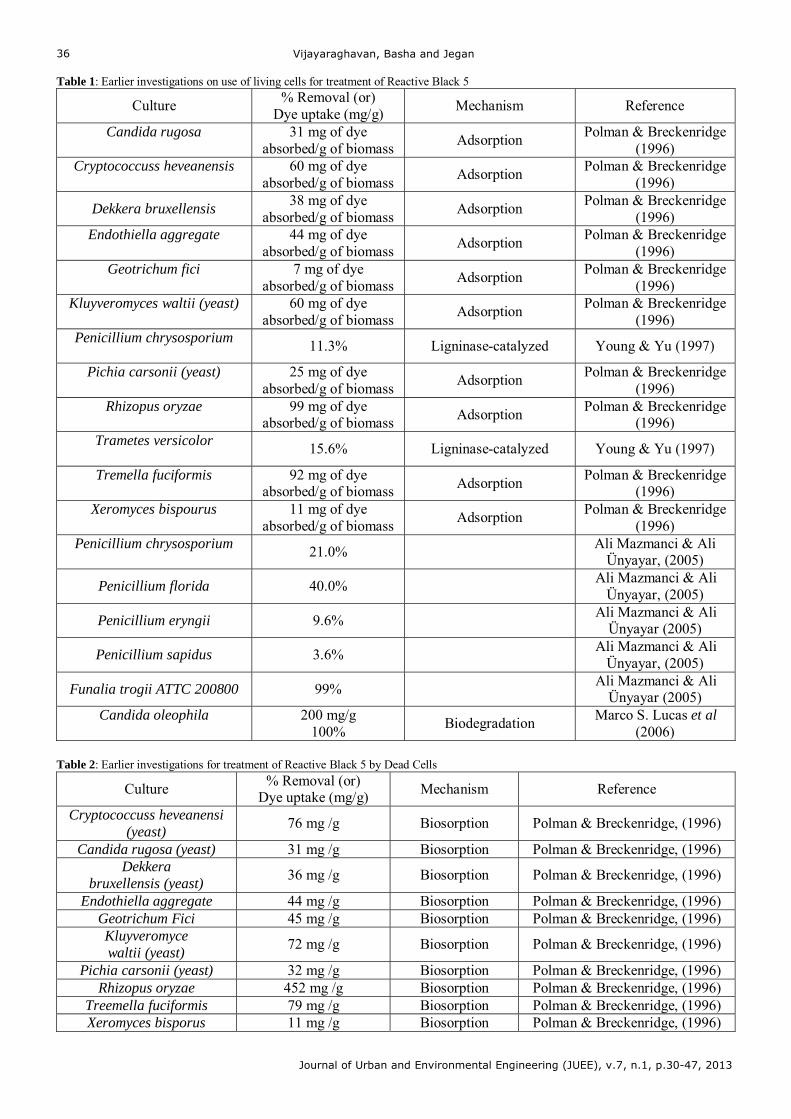
Vijayaraghavan, Basha and Jegan
Journal of Urban and Environmental Engineering (JUEE), v.7, n.1, p.30-47, 2013
36
Table 1: Earlier investigations on use of living cells for treatment of Reactive Black 5
Culture % Removal (or)
Dye uptake (mg/g) Mechanism Reference
Candida rugosa
31 mg of dye absorbed/g of biomass
Adsorption Polman & Breckenridge
(1996) Cryptococcuss heveanensis
60 mg of dye
absorbed/g of biomass Adsorption
Polman & Breckenridge (1996)
Dekkera bruxellensis 38 mg of dye
absorbed/g of biomass Adsorption
Polman & Breckenridge (1996)
Endothiella aggregate
44 mg of dye absorbed/g of biomass
Adsorption Polman & Breckenridge
(1996) Geotrichum fici
7 mg of dye
absorbed/g of biomass Adsorption
Polman & Breckenridge (1996)
Kluyveromyces waltii (yeast)
60 mg of dye absorbed/g of biomass
Adsorption Polman & Breckenridge
(1996) Penicillium chrysosporium
11.3% Ligninase-catalyzed Young & Yu (1997)
Pichia carsonii (yeast)
25 mg of dye absorbed/g of biomass
Adsorption Polman & Breckenridge
(1996) Rhizopus oryzae
99 mg of dye
absorbed/g of biomass Adsorption
Polman & Breckenridge (1996)
Trametes versicolor
15.6% Ligninase-catalyzed Young & Yu (1997)
Tremella fuciformis
92 mg of dye absorbed/g of biomass
Adsorption Polman & Breckenridge
(1996) Xeromyces bispourus
11 mg of dye
absorbed/g of biomass Adsorption
Polman & Breckenridge (1996)
Penicillium chrysosporium
21.0% Ali Mazmanci & Ali
Ünyayar, (2005)
Penicillium florida 40.0% Ali Mazmanci & Ali
Ünyayar, (2005)
Penicillium eryngii 9.6% Ali Mazmanci & Ali
Ünyayar (2005)
Penicillium sapidus 3.6% Ali Mazmanci & Ali
Ünyayar, (2005)
Funalia trogii ATTC 200800 99% Ali Mazmanci & Ali
Ünyayar (2005) Candida oleophila
200 mg/g
100% Biodegradation
Marco S. Lucas et al (2006)
Table 2: Earlier investigations for treatment of Reactive Black 5 by Dead Cells
Culture % Removal (or)
Dye uptake (mg/g) Mechanism Reference
Cryptococcuss heveanensi (yeast)
76 mg /g Biosorption Polman & Breckenridge, (1996)
Candida rugosa (yeast) 31 mg /g Biosorption Polman & Breckenridge, (1996) Dekkera
bruxellensis (yeast) 36 mg /g Biosorption Polman & Breckenridge, (1996)
Endothiella aggregate 44 mg /g Biosorption Polman & Breckenridge, (1996) Geotrichum Fici 45 mg /g Biosorption Polman & Breckenridge, (1996) Kluyveromyce waltii (yeast)
72 mg /g Biosorption Polman & Breckenridge, (1996)
Pichia carsonii (yeast) 32 mg /g Biosorption Polman & Breckenridge, (1996) Rhizopus oryzae 452 mg /g Biosorption Polman & Breckenridge, (1996)
Treemella fuciformis 79 mg /g Biosorption Polman & Breckenridge, (1996) Xeromyces bisporus 11 mg /g Biosorption Polman & Breckenridge, (1996)
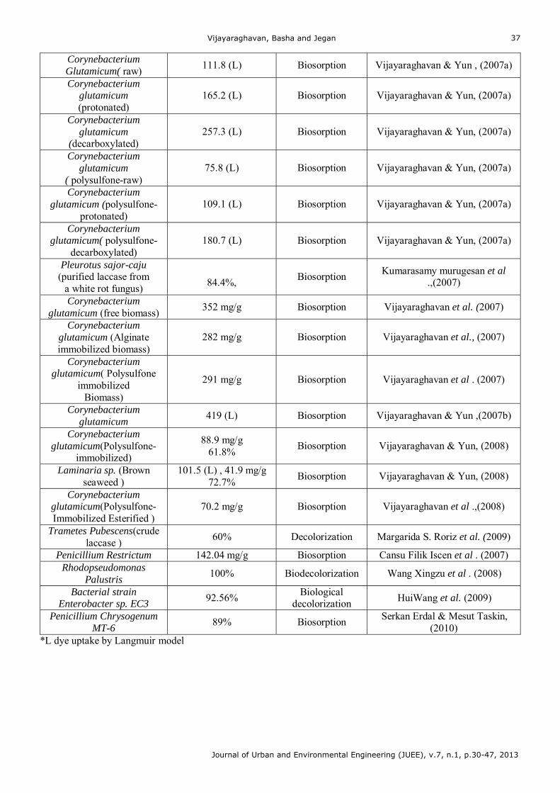
Vijayaraghavan, Basha and Jegan
Journal of Urban and Environmental Engineering (JUEE), v.7, n.1, p.30-47, 2013
37
Corynebacterium Glutamicum( raw)
111.8 (L) Biosorption Vijayaraghavan & Yun , (2007a)
Corynebacterium glutamicum (protonated)
165.2 (L) Biosorption Vijayaraghavan & Yun, (2007a)
Corynebacterium glutamicum
(decarboxylated) 257.3 (L) Biosorption Vijayaraghavan & Yun, (2007a)
Corynebacterium glutamicum
( polysulfone-raw) 75.8 (L) Biosorption Vijayaraghavan & Yun, (2007a)
Corynebacterium glutamicum (polysulfone-
protonated) 109.1 (L) Biosorption Vijayaraghavan & Yun, (2007a)
Corynebacterium glutamicum( polysulfone-
decarboxylated) 180.7 (L) Biosorption Vijayaraghavan & Yun, (2007a)
Pleurotus sajor-caju (purified laccase from
a white rot fungus)
84.4%,
Biosorption Kumarasamy murugesan et al
.,(2007)
Corynebacterium glutamicum (free biomass)
352 mg/g Biosorption Vijayaraghavan et al. (2007)
Corynebacterium glutamicum (Alginate immobilized biomass)
282 mg/g Biosorption Vijayaraghavan et al., (2007)
Corynebacterium glutamicum( Polysulfone
immobilized Biomass)
291 mg/g Biosorption Vijayaraghavan et al . (2007)
Corynebacterium glutamicum
419 (L) Biosorption Vijayaraghavan & Yun ,(2007b)
Corynebacterium glutamicum(Polysulfone-
immobilized)
88.9 mg/g 61.8%
Biosorption Vijayaraghavan & Yun, (2008)
Laminaria sp. (Brown seaweed )
101.5 (L) , 41.9 mg/g 72.7%
Biosorption Vijayaraghavan & Yun, (2008)
Corynebacterium glutamicum(Polysulfone-Immobilized Esterified )
70.2 mg/g Biosorption Vijayaraghavan et al .,(2008)
Trametes Pubescens(crude laccase )
60% Decolorization Margarida S. Roriz et al. (2009)
Penicillium Restrictum 142.04 mg/g Biosorption Cansu Filik Iscen et al . (2007) Rhodopseudomonas
Palustris 100% Biodecolorization Wang Xingzu et al . (2008)
Bacterial strain Enterobacter sp. EC3
92.56% Biological
decolorization HuiWang et al. (2009)
Penicillium Chrysogenum MT-6
89% Biosorption Serkan Erdal & Mesut Taskin,
(2010) *L dye uptake by Langmuir model
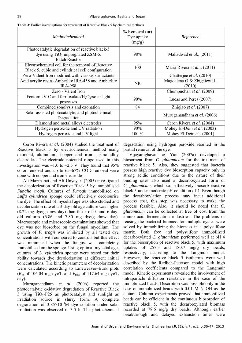
Vijayaraghavan, Basha and Jegan
Journal of Urban and Environmental Engineering (JUEE), v.7, n.1, p.30-47, 2013
38
Table 3: Earlier investigations for treatment of Reactive Black 5 by chemical methods
Method/chemical % Removal (or)
Dye uptake (mg/g)
Reference
Photocatalytic degradation of reactive black-5 dye using TiO2 impregnated ZSM-5.
Batch Reactor 98% Mahadwad et al., (2011)
Electrochemical cell for the removal of Reactive Black 5. cubic and cylindrical cell configuration
100 Maria Rivera et aL., (2011)
Zero-Valent Iron modified with various surfactants Chatterjee et al. (2010) Acid acrylic resins Amberlite IRA-458 and Amberlite
IRA-958 NR
Magdalena G & Zbigniew H, (2010)
Zero - Valent Iron Chompuchan et al. (2009) Fenton/UV-C and ferrioxalate/H2O2/solar light
processes 90% Lucas and Peres (2007)
Combined sonolysis and ozonation 84 Zhiqiao et al. (2007) Solar assisted photocatalytic and photochemical
Degradation Muruganandham et al. (2006)
Diamond and metal alloys electrodes 95% Ceron Rivera et al. (2004) Hydrogen peroxide and UV radiation 90% Mohey El-Dein et al. (2003)
Hydrogen peroxide and UV light 100 % Mohey El-Dein et . (2001)
Ceron Rivera et al. (2004) studied the treatment of Reactive black 5 by electrochemical method using diamond, aluminium, copper and iron - zinc alloy electrodes. The electrode potential range used in this investigation was 1.0 to 2.5 V. They found that 95% color removal and up to 65–67% COD removal were done with copper and iron electrodes.
Ali Mazmanci and Ali Unyayar, (2005) investigated the decolorization of Reactive Black 5 by immobilised Funalia trogii. Cultures of F.trogii immobilised on Luffa cylindrica sponge could effectively decolourise the dye. The effect of mycelial age was also studied and decolorization rate of a 3-day-old age culture was higher (8.22 mg dye/g dmw day) than those of 0- and 6-day-old cultures (6.86 and 7.80 mg dye/g dmw day). Macroscopic and microscopic examinations showed that dye was not biosorbed on the fungal mycelium. The growth of F. trogii was inhibited by all tested dye concentrations with compared to controls but this effect was minimised when the fungus was completely immobilised on the sponge. Using optimal mycelial age, cultures of L. cylindrica sponge were tested for their ability towards dye decolorization at different initial concentrations. The kinetic parameters of decolorization were calculated according to Lineweaver–Burk plots (Km of 106.04 mg dye/L and Vmax of 117.64 mg dye/L day).
Muruganandham et al. (2006) reported the photocatalytic oxidative degradation of Reactive Black 5 using TiO2-P25 as photocatalyst and sunlight as irradiation source in slurry form. A complete degradation of 3.85×10⁻⁴M dye solution under solar irradiation was observed in 3.5 h. The photochemical
degradation using hydrogen peroxide resulted in the partial removal of the dye.
Vijayaraghavan & Yun (2007a) developed a biosorbent from C. glutamicum for the treatment of reactive black 5. Also, they suggested that bacteria possess high reactive dye biosorption capacity only in strong acidic conditions due to the nature of their binding sites also used a decarboxylated form of C. glutamicum, which can effectively biosorb reactive black 5 under moderate pH condition of 4. Even though the decarboxylation process may incur additional process cost, this step was necessary to make the process feasible. Also, it should be noted that C. glutamicum can be collected at free of cost from the amino acid fermentation industries. The problems of reusing the bacterial biomass for multiple cycles were solved by immobilizing the biomass in a polysulfone matrix. Both free and polysulfone immobilized decarboxylated C. glutamicum performed well at pH 4 for the biosorption of reactive black 5, with maximum uptakes of 257.3 and 180.7 mg/g dry beads, respectively, according to the Langmuir model. However, the reactive black 5 isotherms were well described by the Redlich-Peterson model with high correlation coefficients compared to the Langmuir model. Kinetic experiments revealed the involvement of intraparticle diffusion resistance in the case of the immobilized beads. Desorption was possible only in the case of immobilized beads with 0.01 M NaOH as the elutant. Column experiments proved that immobilized beads can be efficient in the continuous biosorption of reactive black 5, with the decarboxylated biomass recorded at 78.6 mg/g dry beads. Although earlier breakthrough and delayed exhaustion times were
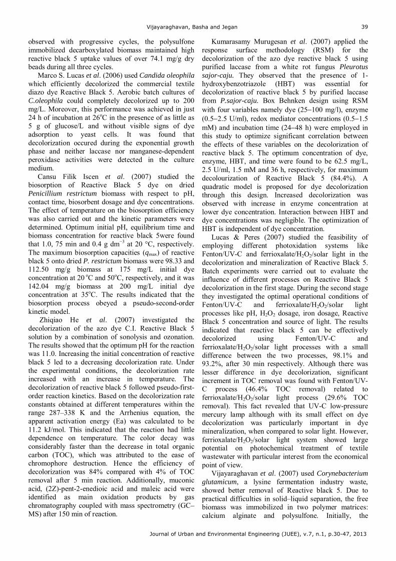
Vijayaraghavan, Basha and Jegan
Journal of Urban and Environmental Engineering (JUEE), v.7, n.1, p.30-47, 2013
39
observed with progressive cycles, the polysulfone immobilized decarboxylated biomass maintained high reactive black 5 uptake values of over 74.1 mg/g dry beads during all three cycles.
Marco S. Lucas et al. (2006) used Candida oleophila which efficiently decolorized the commercial textile diazo dye Reactive Black 5. Aerobic batch cultures of C.oleophila could completely decolorized up to 200 mg/L. Moreover, this performance was achieved in just 24 h of incubation at 26oC in the presence of as little as 5 g of glucose/L and without visible signs of dye adsorption to yeast cells. It was found that decolorization occured during the exponential growth phase and neither laccase nor manganese-dependent peroxidase activities were detected in the culture medium.
Cansu Filik Iscen et al. (2007) studied the biosorption of Reactive Black 5 dye on dried Penicillium restrictum biomass with respect to pH, contact time, biosorbent dosage and dye concentrations. The effect of temperature on the biosorption efficiency was also carried out and the kinetic parameters were determined. Optimum initial pH, equilibrium time and biomass concentration for reactive black 5were found that 1.0, 75 min and 0.4 g dm−3 at 20 °C, respectively. The maximum biosorption capacities (qmax) of reactive black 5 onto dried P. restrictum biomass were 98.33 and 112.50 mg/g biomass at 175 mg/L initial dye concentration at 20 oC and 50oC, respectively, and it was 142.04 mg/g biomass at 200 mg/L initial dye concentration at 35oC. The results indicated that the biosorption process obeyed a pseudo-second-order kinetic model.
Zhiqiao He et al. (2007) investigated the decolorization of the azo dye C.I. Reactive Black 5 solution by a combination of sonolysis and ozonation. The results showed that the optimum pH for the reaction was 11.0. Increasing the initial concentration of reactive black 5 led to a decreasing decolorization rate. Under the experimental conditions, the decolorization rate increased with an increase in temperature. The decolorization of reactive black 5 followed pseudo-first-order reaction kinetics. Based on the decolorization rate constants obtained at different temperatures within the range 287–338 K and the Arrhenius equation, the apparent activation energy (Ea) was calculated to be 11.2 kJ/mol. This indicated that the reaction had little dependence on temperature. The color decay was considerably faster than the decrease in total organic carbon (TOC), which was attributed to the ease of chromophore destruction. Hence the efficiency of decolorization was 84% compared with 4% of TOC removal after 5 min reaction. Additionally, muconic acid, (2Z)-pent-2-enedioic acid and maleic acid were identified as main oxidation products by gas chromatography coupled with mass spectrometry (GC–MS) after 150 min of reaction.
Kumarasamy Murugesan et al. (2007) applied the response surface methodology (RSM) for the decolorization of the azo dye reactive black 5 using purified laccase from a white rot fungus Pleurotus sajor-caju. They observed that the presence of 1-hydroxybenzotriazole (HBT) was essential for decolorization of reactive black 5 by purified laccase from P.sajor-caju. Box Behnken design using RSM with four variables namely dye (25100 mg/l), enzyme (0.52.5 U/ml), redox mediator concentrations (0.51.5 mM) and incubation time (2448 h) were employed in this study to optimize significant correlation between the effects of these variables on the decolorization of reactive black 5. The optimum concentration of dye, enzyme, HBT, and time were found to be 62.5 mg/L, 2.5 U/ml, 1.5 mM and 36 h, respectively, for maximum decolourization of Reactive Black 5 (84.4%). A quadratic model is proposed for dye decolorization through this design. Increased decolorization was observed with increase in enzyme concentration at lower dye concentration. Interaction between HBT and dye concentrations was negligible. The optimization of HBT is independent of dye concentration.
Lucas & Peres (2007) studied the feasibility of employing different photoxidation systems like Fenton/UV-C and ferrioxalate/H2O2/solar light in the decolorization and mineralization of Reactive Black 5. Batch experiments were carried out to evaluate the influence of different processes on Reactive Black 5 decolorization in the first stage. During the second stage they investigated the optimal operational conditions of Fenton/UV-C and ferrioxalate/H2O2/solar light processes like pH, H2O2 dosage, iron dosage, Reactive Black 5 concentration and source of light. The results indicated that reactive black 5 can be effectively decolorized using Fenton/UV-C and ferrioxalate/H2O2/solar light processes with a small difference between the two processes, 98.1% and 93.2%, after 30 min respectively. Although there was lesser difference in dye decolorization, significant increment in TOC removal was found with Fenton/UV-C process (46.4% TOC removal) related to ferrioxalate/H2O2/solar light process (29.6% TOC removal). This fact revealed that UV-C low-pressure mercury lamp although with its small effect on dye decolorization was particularly important in dye mineralization, when compared to solar light. However, ferrioxalate/H2O2/solar light system showed large potential on photochemical treatment of textile wastewater with particular interest from the economical point of view.
Vijayaraghavan et al. (2007) used Corynebacterium glutamicum, a lysine fermentation industry waste, showed better removal of Reactive black 5. Due to practical difficulties in solid–liquid separation, the free biomass was immobilized in two polymer matrices: calcium alginate and polysulfone. Initially, the
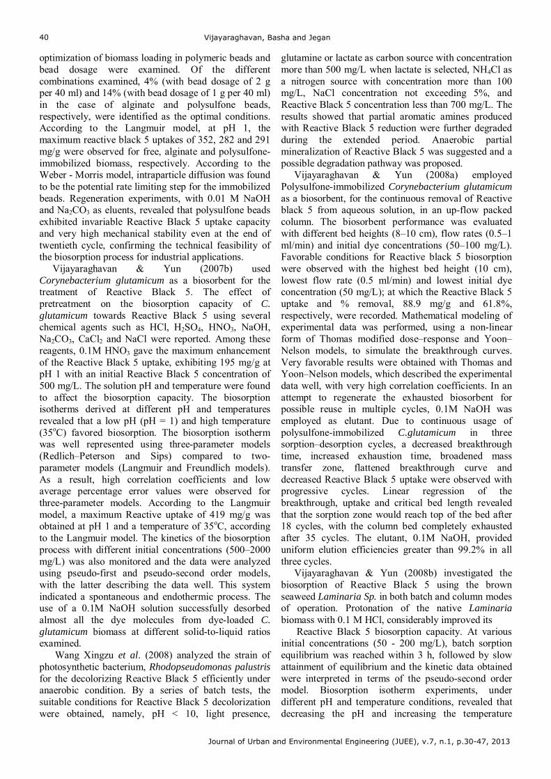
Vijayaraghavan, Basha and Jegan
Journal of Urban and Environmental Engineering (JUEE), v.7, n.1, p.30-47, 2013
40
optimization of biomass loading in polymeric beads and bead dosage were examined. Of the different combinations examined, 4% (with bead dosage of 2 g per 40 ml) and 14% (with bead dosage of 1 g per 40 ml) in the case of alginate and polysulfone beads, respectively, were identified as the optimal conditions. According to the Langmuir model, at pH 1, the maximum reactive black 5 uptakes of 352, 282 and 291 mg/g were observed for free, alginate and polysulfone-immobilized biomass, respectively. According to the Weber - Morris model, intraparticle diffusion was found to be the potential rate limiting step for the immobilized beads. Regeneration experiments, with 0.01 M NaOH and Na2CO3 as eluents, revealed that polysulfone beads exhibited invariable Reactive Black 5 uptake capacity and very high mechanical stability even at the end of twentieth cycle, confirming the technical feasibility of the biosorption process for industrial applications.
Vijayaraghavan & Yun (2007b) used Corynebacterium glutamicum as a biosorbent for the treatment of Reactive Black 5. The effect of pretreatment on the biosorption capacity of C. glutamicum towards Reactive Black 5 using several chemical agents such as HCl, H2SO4, HNO3, NaOH, Na2CO3, CaCl2 and NaCl were reported. Among these reagents, 0.1M HNO3 gave the maximum enhancement of the Reactive Black 5 uptake, exhibiting 195 mg/g at pH 1 with an initial Reactive Black 5 concentration of 500 mg/L. The solution pH and temperature were found to affect the biosorption capacity. The biosorption isotherms derived at different pH and temperatures revealed that a low pH (pH = 1) and high temperature (35oC) favored biosorption. The biosorption isotherm was well represented using three-parameter models (Redlich–Peterson and Sips) compared to two-parameter models (Langmuir and Freundlich models). As a result, high correlation coefficients and low average percentage error values were observed for three-parameter models. According to the Langmuir model, a maximum Reactive uptake of 419 mg/g was obtained at pH 1 and a temperature of 35oC, according to the Langmuir model. The kinetics of the biosorption process with different initial concentrations (500–2000 mg/L) was also monitored and the data were analyzed using pseudo-first and pseudo-second order models, with the latter describing the data well. This system indicated a spontaneous and endothermic process. The use of a 0.1M NaOH solution successfully desorbed almost all the dye molecules from dye-loaded C. glutamicum biomass at different solid-to-liquid ratios examined.
Wang Xingzu et al. (2008) analyzed the strain of photosynthetic bacterium, Rhodopseudomonas palustris for the decolorizing Reactive Black 5 efficiently under anaerobic condition. By a series of batch tests, the suitable conditions for Reactive Black 5 decolorization were obtained, namely, pH < 10, light presence,
glutamine or lactate as carbon source with concentration more than 500 mg/L when lactate is selected, NH4Cl as a nitrogen source with concentration more than 100 mg/L, NaCl concentration not exceeding 5%, and Reactive Black 5 concentration less than 700 mg/L. The results showed that partial aromatic amines produced with Reactive Black 5 reduction were further degraded during the extended period. Anaerobic partial mineralization of Reactive Black 5 was suggested and a possible degradation pathway was proposed.
Vijayaraghavan & Yun (2008a) employed Polysulfone-immobilized Corynebacterium glutamicum as a biosorbent, for the continuous removal of Reactive black 5 from aqueous solution, in an up-flow packed column. The biosorbent performance was evaluated with different bed heights (8–10 cm), flow rates (0.5–1 ml/min) and initial dye concentrations (50–100 mg/L). Favorable conditions for Reactive black 5 biosorption were observed with the highest bed height (10 cm), lowest flow rate (0.5 ml/min) and lowest initial dye concentration (50 mg/L); at which the Reactive Black 5 uptake and % removal, 88.9 mg/g and 61.8%, respectively, were recorded. Mathematical modeling of experimental data was performed, using a non-linear form of Thomas modified dose–response and Yoon–Nelson models, to simulate the breakthrough curves. Very favorable results were obtained with Thomas and Yoon–Nelson models, which described the experimental data well, with very high correlation coefficients. In an attempt to regenerate the exhausted biosorbent for possible reuse in multiple cycles, 0.1M NaOH was employed as elutant. Due to continuous usage of polysulfone-immobilized C.glutamicum in three sorption–desorption cycles, a decreased breakthrough time, increased exhaustion time, broadened mass transfer zone, flattened breakthrough curve and decreased Reactive Black 5 uptake were observed with progressive cycles. Linear regression of the breakthrough, uptake and critical bed length revealed that the sorption zone would reach top of the bed after 18 cycles, with the column bed completely exhausted after 35 cycles. The elutant, 0.1M NaOH, provided uniform elution efficiencies greater than 99.2% in all three cycles.
Vijayaraghavan & Yun (2008b) investigated the biosorption of Reactive Black 5 using the brown seaweed Laminaria Sp. in both batch and column modes of operation. Protonation of the native Laminaria biomass with 0.1 M HCl, considerably improved its
Reactive Black 5 biosorption capacity. At various initial concentrations (50 - 200 mg/L), batch sorption equilibrium was reached within 3 h, followed by slow attainment of equilibrium and the kinetic data obtained were interpreted in terms of the pseudo-second order model. Biosorption isotherm experiments, under different pH and temperature conditions, revealed that decreasing the pH and increasing the temperature
Vijayaraghavan, Basha and Jegan
Journal of Urban and Environmental Engineering (JUEE), v.7, n.1, p.30-47, 2013
41
favored biosorption. According to the Langmuir model, the maximum Reactive Black 5 uptake of 101.5 mg/g was observed at pH 1 and temperature of 40oC. 0.01 M NaOH solution successfully eluted all dye from the Reactive Black 5 -loaded Laminaria biomass. The feasibility of the brown seaweed for the continuous removal of Reactive Black 5 from aqueous solution was examined in an up-flow packed column (1 cm ID and 12 cm height). With a bed height, flow rate and initial Reactive Black 5 concentration at 10 cm, 1 ml/min and 50 mg/L, respectively, the Laminaria biomass exhibited an RB5 uptake and removal efficiency of 41.9 mg/g and 72.7%, respectively. The column was successfully eluted using 0.01 M NaOH with an elution efficiency of 97.7%.
Vijayaraghavan et al. (2008) reported the ability of polysulfone-immobilized esterified Corynebacterium glutamicum for biosorption of Reactive Black 5 and Reactive Orange 16 from single- and dual-dye solutions were investigated. Single-dye biosorption isotherm experiments exposed that polysulfone-immobilized esterified Corynebacterium glutamicum performed well in the biosorption of Reactive Orange 16, with a higher experimental uptake of 248.1 mg/g, compared to 174.1 mg/g for Reactive Black 5. Conversely, the uptake of Reactive Orange 16 was suppressed almost 2.5 times in the presence of Reactive Black 5, whereas polysulfone-immobilized esterified Corynebacterium glutamicum maintained similar Reactive Black 5 uptakes in both single- and dual-dye systems. Several factors might be responsible for this effect, the most important being the number of sulfonate groups and the size of each reactive dye. The continuous biosorption of reactive dyes from single- and dual-dye solutions using an upflow packed column was successful with polysulfone-immobilized esterified Corynebacterium glutamicum being regenerated and reused for three cycles.
Hui Wang et al. (2009) studied the decolorization of the Reactive Black 5 by a bacterial strain Enterobacter sp. EC3. The optimal conditions for the decolorizing activity of Enterobacter sp. EC3 were anaerobic conditions with glucose supplementation, at pH 7.0, and 37oC. The maximum decolorization efficiency against Reactive Black 5 achieved in this study was 92.56%.
Roriz et al. (2009) studied the decolorization of the Reactive Black 5 by crude laccase from the white-rot fungus Trametes pubescens using response surface methodology. The presence of the redox mediator 1-hydroxybenzotriazole greatly improved the decolorization levels of Reactive Black 5 by crude laccase from T.Pubescens. The optimum concentrations of 1-hydroxybenzotriazole, Reactive Black 5 and laccase were 1.17mM, 150 mg/L and 500 U/l, respectively, for a maximum decolorization of Reactive Black 5 (about 60% in 20 min).
Chompuchan et al. (2009) used the nanoscale zero valent iron (NZVI) to decolorize Reactive Black 5 and
Reactive Red 198 in synthesized wastewater and investigated the effects of the iron particle size, iron dosage and solution pHs on the destruction of reactive black 5 and RR198. The removal kinetic rates (kobs) of RB5 (0.0109 min-1) and RR198 (0.0111 min-1) by 0.5% NZVI were many times higher than those of microscale zerovalent iron (ZVI) (0.0007 min-1 and 0.0008 min-1, respectively). The iron dosage increment exponentially increased the removal efficiencies of both Reactive Black 5 and RR198. Additionally, lowering pH from 9 to 5 increased the decolorization kinetic rates of both reactive black 5 and RR198 by NZVI. The destruction of azo bond (N=N) in the chromospheres of both reactive dyes led to decolorization of dye solutions.
Greluk & Hubicki (2010) used strongly basic acrylic anion exchangers namely Amberlite IRA-458 and Amberlite IRA-958 for the removal of Reactive Black 5. Adsorption experiments indicated that the amount of the dye adsorbed on both Amberlite IRA-458 and Amberlite IRA-958 were dependent on the initial dye concentration in the range of 50–500 mg/L. Modeling of kinetic results showed that the sorption process of the dye adsorption on both anion exchangers was best described by the pseudo second-order kinetic model in the investigated concentration domain. The effect of temperature on dye removal showed that the maximum capacity was obtained at 318 and 308 K for the dye adsorption on Amberlite IRA-458 and Amberlite IRA-958, respectively. The adsorption isotherm data were fitted well to the Langmuir isotherm and according to this model, Amberlite IRA-458 and Amberlite IRA-958 exhibited the highest monolayer sorption capacity of 1295.93 and 1723.964 mg/g.
Chatterjee et al. (2010) used Zero Valent Iron (ZVI) particles for the reductive degradation of Reactive Black 5 in aqueous solution. The sizes of the synthesized ZVI particles were in the microscale range, with an average diameter of 13.57μm. The efficiency of surfactant-treated ZVI particles for the decolorization of reactive black 5 solution was studied with three different surfactants namely Triton X-100, Cetyl Trimethyl Ammonium Bromide and Sodium Dodecyl Sulfate. The normalized residual concentration after decolorization of 500 mg/L Reactive Black 5 by ZVI for 3 h was 0.236, while ZVI particles treated with Triton X-100 (0.5 g/L), Cetyl Trimethyl Ammonium Bromide (CTAB) (1.0 g/L), and Sodium Dodecyl Sulfate (SDS) (2.5 g/L) exhibited normalized residual concentration of 0.172, 0.154, and 0.393, respectively, after 3 h. The color removal efficiency was found to be increased with the decrease in initial pH of dye solution and ZVI exhibited good color removal efficiency at acidic pH. Decolorization kinetics by pseudo-first-order rate equation showed that removal rate was increased after treatment with Triton X-100 as well as CTAB, while that was reduced after SDS treatment.
Vijayaraghavan, Basha and Jegan
Journal of Urban and Environmental Engineering (JUEE), v.7, n.1, p.30-47, 2013
42
Karatas et al. (2010) investigated the efficiency of the sequential anaerobic - aerobic system for decolorization of Reactive Black 5. The synthetic wastewater contained 150 mg/L dye and 3000 mg/L glucose-COD. An upflow anaerobic sludge blanket (USAB) (CSAR) reactor and continuously stirred aerobic reactors were used to remove color and COD. The methane gas production efficiencies were also investigated under the anaerobic conditions. The UASB - CSAR were operated at different organic loading rates (2.422.5 Kg COD/m3·day) and hydraulic retention times (3.2 - 30.1 h). The COD removal efficiencies decreased from 61 to 36.7% with increases in organic loadings from 2.4 to 22.5 Kg COD/m3/day in the anaerobic UASB reactor. The color removal decreased from 99.8 to 90.7% when the hydraulic retention time decreased from 30.1 to 3.2 hours. The methane production efficiencies obtained were 75 and 38.3% at the organic loading rates of 2.4 and 22.5 Kg COD/m3
day respectively. The effects of both sludge retention times and the food/mass (F/M) ratio on the COD removal efficiencies were investigated in the aerobic reactor. COD removal efficiencies of 62.2 and 86.3% were obtained at 2 and 19 days sludge retention time in the aerobic reactor. The COD removal efficiencies were found to be 86.3 and 62.2% at F/M ratios of 0.112 and 1.569 Kg COD/Kg day. The color and COD removal efficiencies obtained were 99.8% and 95% by using 150 mg/L of Reactive Black 5 dye concentration in the sequential anaerobic aerobic reactor.
Erdal & Taskin (2010) reported the decolorization of Reactive Black 5 by Penicillium chrysogenum MT-6. Dye uptake was strongly depended on mycelial morphology. Small uniform pellets with 2 mm size and nutrient-poor medium were found to be better for dye uptake. Optimal conditions for dye uptake were determined as initial pH of 5.0, shaking speed of 150 rpm, temperature of 28°C, spore concentration of 107/ml, 10 g/L sucrose and 1 g/L ammonium chloride. The maximum removal/uptake of dye by fungus was 89% (0.267 g removed-dye) with 3.83 g/L of biomass production at an initial dye concentration of 0.3 g/L in 100 h. The fungus was found to be a good bio-system for the decolorization of the medium containing Reactive Black-5.
Rivera et al. (2011) studied the decolorization of Reactive Black 5 by an electrochemical technology in both cubic and cylindrical cell configurations. Low decolorization was detected in the treatment of pure solutions of Reactive Black 5, but a significant extent of decolorization was observed in the presence of Na2SO4. The extent of decolorization was largely dependent on the cell configuration and the best results were obtained when the cylindrical cell was employed. Nearly complete decolorization was achieved in 3 h for an effluent containing 70 mg/L Reactive Black 5 and 0.1 M Na2SO4 and the TOC removal was approximately 95%.
In the presence of the non-inert electrolyte NaCl, the complete decolorization was detected. However, due to the chloro-organic compounds formed in the electrochemical oxidation with NaCl, the TOC removal in the most optimal condition was approximately 93%.
Mahadwad et al. (2011) studied the photocatalytic degradation of Reactive Black 5 using supported TiO2 photocatalyst based adsorbent as a semiconductor photocatalyst in a batch reactor. The synthesized photocatalyst composition was developed using TiO2 as photoactive component and zeolite (ZSM-5) as the adsorbent. The optimum formulation of supported catalyst was found to be (TiO2: ZSM-5 = 0·15:1) which gave the highest efficiency with 98% degradation of 50 mg/L reactive black 5 solution in 90 min. The reduction in the chemical oxygen demand (COD, 88%) proves the mineralization of the Reactive Black 5 dye along with the colour removal. The supported TiO2 was found to be stable for repeated use.
CONCLUSION This review makes a simple comparison among various physicochemical methods namely photo catalysis, electrochemical, adsorption, hydrolysis and biological methods such as biosorption and bioaccumulation and also discussed the merits and demerits of these methods involved in the decolorization of reactive black 5.
The main disadvantages of the physical methods such as adsorption, ion exchange and membrane filtration were that they simply transfer the dye molecules to another phase rather than destroying them and they are effective only when the effluent volume is small.
The main disadvantage of the chemical methods such as chemical oxidation, electrochemical degradation and ozonation were the requirements of an effective sludge producing pretreatment. Also, these chemical methods with high cost were rarely used in the actual treatment process and the disposal of sludge containing chemicals at the end of treatment requires further use of chemicals.
Conventional water treatment technologies such as solvent extraction, activated carbon adsorption and chemical treatment process such as oxidation by ozone (O3) often produce hazardous by-products and generate large amount of solid wastes, which require costly disposal or regeneration method.
The requirement of chemicals and the temperature to carry the electro chemical reaction was less than those of other equivalent non-electrochemical treatment. It can also prevent the production of unwanted side products. But if suspended or colloidal solids were high in concentration in the waste water, they slow down the electrochemical reaction. Therefore, those materials need to be sufficiently removed before electrochemical oxidation.
Vijayaraghavan, Basha and Jegan
Journal of Urban and Environmental Engineering (JUEE), v.7, n.1, p.30-47, 2013
43
Compared to the conventional methods, application to recalcitrant materials, operation at high and low contaminant concentrations over a wide range of pH, temperature and salinity range, biomass acclimatization is irrelevant and straight forward process control are the potential advantages of the enzymatic treatments.
Biodegradation, Bioaccumulation and biosorption were the three main technologies used in biological dye removal process. They possess good potential to replace conventional methods for the treatment of dye bearing industry effluents. Biological processes can be carried out in situ at the contaminated site, these were usually environmentally benign i.e., no secondary pollution and they were cost effective. These were the principle advantages of biological technologies for the treatment of dye industry effluents. Hence in recent years, research attention has been focused greatly on biological methods for the treatment of effluents. The disadvantage of the degradation process is that it suffers from low degradation efficiency or even no degradation for some dyes and practical difficulty in continuous process. The important disadvantage bioaccumulation process is using living organism, which is not advisable for the continuous treatment of highly toxic effluents. This problem can be overcome in biosorption by the use of dead biomass, which is flexible to environmental conditions and toxicant concentrations.
By considering all the above said factors, as a researcher, our prime aim is to find out the environmental benign technique to remove hazardous materials from environment. In this concern, from the literature we conclude that, the biosorption is harmless and cost effective method to achieve this goal and also this technique will not produce any secondary pollutants. The natural materials like marine algae, waste materials from industry and agriculture waste are very much useful in the process of removing the pollutants as biosorbent. Thus we proposed that, the biosorption is an opt method to remove the toxicants. REFERENCES Acuner, E. & Dilek, F.B. (2004) Treatment of tectilon yellow
2G by Chlorella vulgaris, Process Biochem. 39(6), 623–631.
Ahmad, A.L., Puasa, S.W. (2007) Reactive dyes decolourization from an aqueous solution by combined coagulation/micellar–enhanced ultrafiltration process, Chem. Eng. J. 132(2), 257–265.
Mazmanci, A. & Ünyayar, A. (2005) Decolorization of Reactive Black 5 by Funalia trogii immobilised on Luffa cylindrica sponge, Process Biochem. 40(1), 337–342.
Aksu, Z. (2005) Application of biosorption for the removal of organic pollutants: a review, Process Biochem, 40, 997–1026
Aksu, Z., Donmez, G. (2005) Combined effects of molasses sucrose and reactive dye on the growth and dye bioaccumulation properties of Candida tropicalis, Process Biochem. 40(12), 2443–2454 .
Aksu, Z., Kilic, N.K. & Ertugrul, S. (2007) Inhibitory effects of chromium(VI) and Remazol Black B on chromium(VI) and dyestuff removals by Trametes versicolor, Enzyme and Microbial Tech. 40, 1167–1174
Alessi, D.S. & Li, Z. (2001) Synergistic effect of cationic surfactants on perchloroethylene degradation by zero–valent iron, Environ. Sci. Technol. 35 ,3713–3717.
Anbia, M., Hariri, S.A. (2010), Removal of methylene blue from aqueous solution using nanoporous SBA–3, Desalination 261 61–66.
Aravindhan, R., Rao, J.R., Nair, B.U. (2007) Removal of basic yellow dye from aqueous solution by sorption on green alga Caulerpa scalpelliformis, J. Hazard. Mater. 142(1) ,68–76.
Atkinson, B.W., Bux, F., Kasan, H.C. (1998) Considerations for application of biosorption technology to remediate metal–contaminated industrial effluents. Water SA 24(1), 129–135.
Axelsson, J., Nilsson, U., Terrazas, E. (2006) Decolorization of the textile dyes Reactive Red 2 and Reactive Blue 4 using Bjerkandera sp. Strain BOL 13 in a continuous rotating biological contactor reactor, Enzyme and Microbial Technology, 39, 32–37
Banat, I.M., Nigam, P., Singh, D., Marchant, R. (1996) Microbial decolorization of textile–dye containing effluents: a review. Bioresour. Technol. 58(2), 217–227.
Barakat, H. (2010) Adsorption and photodegradation of procion Yellow H–Exl Dyes in textile wastewater over Tio2 Suspension. Proc. International Water Technology Conference, Cairo, Egypt.
Barsanescu, A., Buhaceanu, R., Dulman. V. (2009) Removal of Basic Blue 3 by sorption onto a weak acid acrylic resin. J. Appl. Polym. Sci. 113(6), 607–614.
Bayramoglu G, B. Altinas, M.Y. Arica (2009) Adsorption kinetics and thermodynamic parameters of cation–exchange resin. Chem. Eng. J. 152(3), 339– 346.
Bilgic, H., Gokcay, C.F., Hasirci, N. (1997) Color removal by white–rot fungi. In: Wise, D.L. (Ed.), Global Environmental Biotechnology. Elsevier, UK, 211–222
Brown M A and De Uito S C (1993) Predicting azo dye toxicity, Crit Rev Environ Sci Technol, 23, 249–324
Cammarota, M.C., Sant Anna Jr., G.L. ( 1992) Decolorization of kraft bleach plant E1stage effluent in a fungal bioreactor. Environ. Technol. 13(1), 65–71
Cansu Filik Iscen, Ismail Kiran, Semra Ilhan (2007) Biosorption of Reactive Black 5 dye by Penicillium restrictum: the kinetic study, J. Hazard. Materials 143(1–2), 335–340
Carliell CM, Barclay SJ, Naidoo N, Buckley CA, Mulholland DA, Senior E (1995) Microbial decolourasition of a reactive azo dye under anaerobic conditions. Water SA 21(1), 61–69.
Ceron, R.M., Davila, M.M., Elizalde, G.M.P. (2004) Degradation of the textile dyes Basic yellow 28 and Reactive black 5 using diamond and metal alloys electrodes, Chemosphere 55(1), 1–10.
Chang, M.–C., Shu, H.–Y., Yu, H.–H., Sung, Y.–C. (2006) Reductive decolourization and total organic carbon reduction of the diazo dye Cl Acid Black 24 by zero–valent iron powder, J. Chem. Technol. Biotechnol. 81, 1259–1266.
Chatterjee, S., Lee, D.S., Lee, M.W., Woo, S.H. (2009a) Congo red adsorption from aqueous solutions by chitosan
Vijayaraghavan, Basha and Jegan
Journal of Urban and Environmental Engineering (JUEE), v.7, n.1, p.30-47, 2013
44
hydrogel beads impregnated with nonionic or anionic surfactant. Bioresour. Technol. 100, 3862–3868.
Chatterjee, S., Lee, M.W., Woo, S.H. (2009b) Influence of impregnation of chitosan beads with cetyl trimethyl ammonium bromide on their structure and adsorption of congo red from aqueous solutions. Chem. Eng. J. 155 , 254–259.
Chatterjeea, S., Limb, S.–R., Woo, S.H. (2010) Removal of Reactive Black 5 by zero–valent iron modified with various surfactants, Chem. Engin. J. 160(1), 27–32.
Cho, H.–H., Park, J.–W. (2006) Sorption and reduction of tetrachloroethylene with zero valent iron and amphiphilic molecules, Chemosphere, 64, 1047–1052.
Chompuchan, T., Satapanajaru, P., Suntornchot, Pengthamkeerati, P. (2009) Decolorization of Reactive Black 5 and Reactive Red 198 using nanoscale zerovalent iron. World Academy of Science, Engineering and Technology 49.
Colindres, H. Yee–Madeira, E. Reguera (2010) Removal of Reactive Black 5 from aqueous solution by ozone for water reuse in textile dyeing processes. Desalination 258(1), 154–158
Crini G (2006) Non–conventional low–cost adsorbents for dye removal: a review, Bioresour. Technol. 97, 1061–1085.
Daneshvar N, Ayazloo M, Khataee AR, Pourhassan M (2007) Biological decolorization of dye solution containing Malachite Green by microalgae Cosmarium sp. Bioresour Technol. 98, 1176–1182
Davila–Jimenez, M.M., Elizalde–Gonzalez, M.P., Gutierrez– Gonzalez, A., Pelaez–Cid, A.A. (2000) Electrochemical treatment of textile dyes and their analysis by high performance liquid chromatography with diode array detection. J. Chromatogr. 889, 253–259.
DeFazio, S.A.K., Lemley, A.T. (1999) Electrochemical treatment of acid dye systems: sodium meta–bisulphite addition to the Andco system. J. Environ. Sci. Health, Part A 34(2), 217–240.
Delee, W., O’Neill, C., Hawkes, F.R., Pinheiro, H.M. (1998) Anaerobic treatment of textile effluents: A review. J. Chem. Technol. Biotechnol. 73(3), 323–335.
Demiral, H., Demiral, I., Karabacakoðlu, B., Tümsek, F. (2008) Adsorption of Textile Dye onto Activated Carbon Prepared from Industrial Waste by ZnCl2 Activation. J. Int. Environm. Appl. Sci. 3(3), 381–389.
Dulman, V.C., Simion, A.. Barsanescu, I., Bunia, V. (2009) Adsorption of anionic textile dye Acid Green 9 from aqueous solution onto weak or strong base anion exchangers. J. Appl. Polym. Sci. 113(6), 615–627.
Duran, N., Esposito, E. (2000) Potential applications of oxidative enzymes and phenoloxidase–like compounds in wastewater and soil treatment: a review. Appl. Catal. B: Environ. 28(1), 83–99.
Easton, J.R. (1995) The dye maker's view. In: Cooper, P. (ed.), Colour in Dyehouse Effluent,Society of Dyehouse and Color, Bradford, England, 9–21
El–Dein, A.M., Libra, J.A., Wiesmann, U. (2003) Mechanism and kinetic model for the decolorization of the azo dye Reactive Black 5 by hydrogen peroxide and UV radiation. Chemosphere 52, 1069–1077.
El Qada E N, S.J. Allen, G.M. Walker (2008) Adsorption of basic dyes from aqueous solution onto activated carbons” , Chem. Eng. J. 135 174–184.
Erdal S and Taski M, (2010) Uptake of textile dye Reactive Black–5 by Penicillium chrysogenum MT–6 isolated from cement–contaminated soil. African J. Microb. Res. 4(8), 618–625,
Eren Z and Acar F N (2006) Adsorption of Reactive Black 5 from an aqueous solution: equilibrium and kinetic studies. Desalination, 194(1), 1–10.
Fan, J., Guo, Y., Wang, J., Fan, M. (2009) Decolorization of azo dye methyl orange in aqueous solution by nanoscale zerovalent iron particles. J. Hazard. Mater. 166(1), 904–910.
Forgacs, E., Cserháti, T., Oros, G. (2004) Removal of synthetic dyes from waste waters: a review. Environ Int. 30(9), 953–971
Fu, Y., Vijaraghavan, T. (2001) Fungal Decolorization of Dye Wastewaters: A Review. Bioresource Technol. 79(2), 251–262
Galindo, C., Kalt, A. (1998) UV–H2O2 oxidation of mono azo dyes in aqueous media: a kinetic study. Dyes Pigm. 40(1), 27–35.
Gallagher, K.A., Healy, M.G., Allen, S.J. (1997) Biosorption of synthetic dye and metal ions from aqueous effluents using fungal biomass. In: Wise, D.L. (Ed) Global Environmental Biotechnology, Elsevier, 27–50.
Glenn, J.K., Gold, M. (1983) Decolorization of several polymeric dyes by the lignin–degrading basidiomycete Phanerochaete chrysosporium. Appl. Environ. Microbiol. 45, 1741–1747.
Goheen, S.C., Durham, D.E., McCulloch, M., Heath, W.O. (1994) The degradation of organic dyes by Corona discharge.In: Eckenfelder, W.W., Bowers, A.R., Roth, J.A. (Eds.), Chemical Oxidation, v Technomic Publishing Co. Inc., Lancaster, Basel,2, 356–367.
Gottlieb A, Shaw C, Smith A, Wheatley A, Forsythe S (2003) The toxicity of textile reactive azo dyes after hydrolysis and decolorization, J. Biotechnol. 101(1), 49–56.
Greluk, M., Hubicki, F. (2010) Kinetics, isotherm and thermodynamic studies of Reactive Black 5 removal by acid acrylic resins. Chem. Engin. J. 162(1), 19–926.
Gutierrez, M.C., Pepio, M., Crespi, M., Mayor, N. (2001) Control factors in the electrochemical oxidation of reactive dyes. Color Technol. 117(3), 356–361.
Hao, O.J., Kim, H., Chiang. P.C. (2000) Decolorization of wastewater. Critical Rev. Environm. Sci. Technol. 30(4), 449–505
He, Z., Song, S., Zhou, H., Ying, H., Chen, J. (2007) C.I. Reactive Black 5 decolorization by combined sonolysis and ozonation, Ultrasonics Sonochemistry 14(2), 298–304.
Heinfling A, Bergbauer M and Szewzyk U (1997) Biodegradation of azo and phthalocyanine dyes by Trametes Versicolor and Bjerkandera adusta, Appl Microbiol Biotechnol, 48, 261
Hui, W., Zheng, X.–W., Su, J.–Q., Tian, Y., Xiong, X.–J., Zheng, T.–L. (2009) Biological decolorization of the reactive dyes Reactive Black 5 by a novel isolated bacterial strain Enterobacter sp. EC3. J. Hazard. Mater. 171(1–3), 654–659.
Ince, N.H. (1999) Critical effect of hydrogen peroxide in photochemical dye degradation, Water Res. 33, 1080–1084.
Iscen C F, Kiran I and Ilhan S (2007) Biosorption of Reactive Black 5 dye by Penicillium restrictum: The kinetic study. J. Hazard. Mater 143(3), 335–340.
Vijayaraghavan, Basha and Jegan
Journal of Urban and Environmental Engineering (JUEE), v.7, n.1, p.30-47, 2013
45
Isýk, M., Sponza, D.T. (2004) Simüle Tekstil Atýksuyunun Anaerobik/Aerobik Arýtýmý, Ekoloji, 14(1), 1–8.
Jia, J., Yang, J., Liao, J., Wang, W., Wang, Z. (1999) Treatment of dyeing wastewater with ACF electrodes. Water Res. 33, 881–884.
Kalyani, D.C., Patil, P.S., Jadhav, J.P., Govindwar, S.P. (2007) Biodegradation of reactive textile dye Red BLI by an isolated bacterium Pseudomonas sp. SUK1, Bioresour Technol. 99, 4635–4641
Kapdan, IK, Oztekin, R. (2006) The effect of hydraulic residence time and initial COD concentration on color and COD removal performance the anaerobic–aerobic SBR system. J. Hazard. Mater. 136(8), 896–901.
Kapoor, A.,Viraraghavan, T. (1995) Fungal biosorption –an alternative treatment option for heavy metal bearing wastewater: a review. Bioresource Technol. 53, 195–206
Karatas, M., Dursun, S., Argun, M.E. (2010) The Decolorization of Azo Dye Reactive Black 5 in a Sequential Anaerobic–Aerobic System, Ekoloji, 74(1), 15–23
Karcher, S., Kornmuller, A., Jekel, M. (2001) Cucurbituril for water treatment. Part I: Solubility of cucurbituril and sorption of reactive dyes. Water Res. 35(14), 3309−3316.
Karcher, S., Kornmuller, A., Jekel, M. (2002b) Anion exchange resins for removal of reactive dyes from textile wastewaters, Water Res. 36 4717–4724.
Khehra MS, Saini HS, Sharma DK, Chadha BS, Chimni SS (2006) Biodegradation of azo dye C.I. Acid Red 88 by anoxic–aerobic sequential bioreactor, Dyes Pigments 70(1), 1–7.
Kobya, M., Can, O.T., Bayramoglu, M. (2003) Treatment of textile wastewaters by electrocoagulation using iron and aluminium electrodes, J. Hazard. Mater, 100, 163–178.
Kumarasamy Murugesan K, Dhamija A, Nam IH, Kim YM, Chang YS (2007) Decolourization of reactive black 5 by laccase: Optimization by response surface methodology. Dyes Pigm. 75, 176–184.
Labanda, J., Sabaté, J., Llorens, A. (2009) Modeling of the dynamic adsorption of an anionic dye through ion–exchange membrane adsorber. J. Membr. Sci. 340(2), 234–240.
Lankinen, V.P., Inkeroinen, M.M., Pellinen, J., Hatakka, A.I. (1991) The onset of lignin–modifying enzymes, decrease of AOX and color removal by white rot fungigrown on bleach plant effuents. Water Sci. Technol. 24(3–4), 189–198.
Lee, Y.H., Pavlostathis, S.G. (2004) Decolorization and toxicity of reactive anthraxquinone textile dyes under methanogenic conditions. Water Res. 38, 1838–1852.
Li, Q, Yue Q –Y, Su, Y., Gao, B.–Y., Li, J. (2009) Two–step kinetic study on the adsorption and desorption of reactive dyes at cationic polymer/bentonite. J. Hazard Mater. 165, 1170–1178
Lin, S.H., Peng, F.C. (1994) Treatment of textile wastewater by electrochemical methods. Water Res. 28(2), 277–282
Peres, L.J.A. (2007) Degradation of Reactive Black 5 by Fenton/UV–C and ferrioxalate/H2O2/solar light processes. Dyes Pigm. 74(6), 622–629.
Malik, PK. (2004) Dye removal from wastewaters using activated carbon developed from sawdust: adsorption equilibrium and kinetics. J. Hazard. Mater. 113, 81–88.
Lucas, M.S., Amaral, C., Sampaio, A., Peres, J.A., Dias, A.A (2006) Biodegradation of diazo dye Reactive Black 5 by a
wild isolate of Candida oleophila. Enzyme Microb. Technol. 39(1), 51–55.
Mahadwad, O.K., Parikh, P.A., Jasra, R.V., Patil, C. (2011) Photocatalytic degradation of reactive black–5 dye using TiO2 impregnated ZSM–5, Bull. Mater. Sci., 34( 3), 551–556.
Mahony, T.O., Guibal, E., Tobin, J.M. (2002) Reactive dye biosorption by Rhizopus arrhizus biomass. Enzyme Microbial Technol. 31, 456–463.
Manu, B., Chaudhari, S. (2002) Anaerobic decolorisation of simulated textile wastewater containing azo dyes. Bioresour Technol. 82, 225–231.
Roriz, M.S., Teixeira, J.F.O., Couto, S.R. (2009) Application of response surface methodological approach to optimise Reactive Black 5 decolouration by crude laccase from Trametes pubescens. J. Hazard. Mater. 169(1–3), 691–696.
Greluk, M., Hubicki, Z. (2010) Kinetics, isotherm and thermodynamic studies of Reactive Black 5 removal by acid acrylic resins. Chem. Engin. J. 162(3), 919–926.
Rivera, M., Pazos, M., Sanromán, M.A. (2011) Development of an electrochemical cell for the removal of Reactive Black 5, Desalination 274(1), 39–43.
Martínez, H.C.A., Brillas, E. (2009) Decontamination of wastewaters containing synthetic organic dyes by electrochemical methods: a general review. Appl Catal B Environ. 87, 105–145
Mazmanci, M.A., Ünyayar, A. (2005) Decolorization of Reactive Black 5 by Funalia trogii immobilised on Luffa cylindrica sponge. Proc. Biochem. 40(1), 337–342
McClung, S.M., Lemley, A.T. (1994) Electrochemical treatment and HPLC analysis of wastewater containing acid dyes. Text. Chem. Colorist. 26(1), 17–22.
Mcmullan, G., C. Meehan, A. Conneely, N. Nirby, P. Robinson, I. Nigam, M. Bannat and S.W.F. Marchant, (2001) Mini review: Microbial decolorization and degradation of textile dyes. Appl. Microbiol. Biotechnol. 56(1), 81–87
Mendez–Paz, D., Omil, F., Lema, J.M. (2005) Anaerobic treatment of azo dye Acid Orange 7 under fedbatch and continuous conditions. Water Res. 39(7), 771–778.
Mishra, G., Tripathy, M. ( 1993) A critical review of the treatment for decolorization of textile effluent, Colourage, 40(1), 35–38.
Mohey El–Dein, A., Libra, J. A., Wiesmann, U. (2001) Kinetics of decolorization and mineralization of the azo dye Reactive Black 5 by hydrogen peroxide and UV Light. Water Sci. Technol. 44(5), 295–301.
Mohey El–Dein.A , J.A. Libra, U. Wiesmann (2003) Mechanism and kinetic model for the decolorization Of the azo dye Reactive Black 5 by hydrogen peroxide and UV radiation, Chemosphere 52, 1069–1077
Morais L.C., Freitas O.M., Gonc_alves E.P., Vasconcelos L.T., Gonzalez Beca C.G ( 1999) Reactive dyes removal from wastewaters by adsorption on Eucalyptus bark: variables that define the process. Water Res. 33(9), 979– 988.
Moussavi G, M. Mahmoudi (2009) Degradation and biodegradability improvement of the reactive red 198 azo dye using catalytic ozonation with MgO nanocrystals. Chem. Eng. J. 152(1), 1–7.
Vijayaraghavan, Basha and Jegan
Journal of Urban and Environmental Engineering (JUEE), v.7, n.1, p.30-47, 2013
46
Muruganandham, N. Sobana, M. Swaminathan (2006) Solar assisted photo catalytic and photochemical degradation of Reactive Black 5. J. Hazard. Mater. 137(3), 1371–1376.
Karataþ, M., Dursun, P., Argun, M.E. (2010) The Decolorization of Azo Dye Reactive Black 5 in a Sequential Anaerobic–Aerobic. System Ekoloji ,19, 74–82.
Ollikka P, Alhonma¨ki K, Leppa¨nen VM, Glumoff T, Raijola T, Suominen I (1993) Decolorization of azo, triphenyl methane, heterocyclic, and polymeric dyes by lignin peroxidase isoenzymes form Phanerochaete chrysosporium. Appl Environ Microbiol. 59, 4010–4016
Osugi M E, K. Rajeshwar, E.R.A. Ferraz, D.P. de Oliveira, Â.R. Araújo, M.V.B. Zanoni (2009) Comparison of oxidation efficiency of dispersed dyes by chemical and photoelectrocatalytic chlorination and removal of mutagenic activity. Electrochim. Acta 54, 2086–2093.
Ozcan A S and Ozcan A (2004) Adsorption of acid dyes from aqueous solutions onto acid–activated bentonite, J Colloid Interf Sci, 276, 39– 46.
Pasti–Grigsby MB, Paszczynski A, Goszczynski S, Crawford DL, Crawford R L (1992) Influence of aromatic substitution patterns on azo dye degradability by Streptomyces spp. and Phanerochaete chrysosporium. Applied Environm. Microb. 58, 3605–3613.
Pearce, C.I., Lloyd, J.R., Guthrie, J.T. (2003) The removal of colour from textile wastewater using whole bacterial cells: a review. Dyes Pigm. 58(1), 179–196.
Philippe C, Vandevivere B and Willy V (1998) Treatment and Reuse of waste water from the textile wet processing industry : Review of emerging Technologies, J. Chem. Technol. Biotechnol. 72, 289–302
Polman, J.K., Breckenridge, C.R. (1996) Biomass mediated binding and recovery of textile dyes from waste effluents. Textile Chemist Colorist. 28(4), 31–35
Powell, W.W., Michelsen, D.L., Boardman, G.D., Dietrich, A.M., Woodby, R.M. (1994) Removal of color and TOC from segregated dye discharges using ozone and Fenton’s reagent. In: Eckenfelder, W.W., Bowers, A.R., Roth, J.A. (Eds.), Chemical Oxidation, vol. 2. Technomic Publishing Co. Inc., Lancaster, Basel, 278–300.
Prasad, M.N.V. and H. Freitas (2003) Metal hyperaccumulation in plants – Biodiversity prospecting for phytoremediation technology. Electronic J. Biotechnol. 6(3), 275–321
Tatarko, M., Bumpus, J.A. (1998) Biodegradation of Congo Red by Phanerochaetechrysosporium. Water Res. 32(5), 1713–1717.
Razo–Flores E, Donlon BA, Field JA, Lettinga G. (1996) Biodegradability of N–substituted aromatics and alkylphenols under methanogenic conditions using granuler sludge. Water Sci. Technol. 33, 47–57.
Renganathan, S., Kalpana, J., Kumar, M., Velan, M. (2009) Equilibrium and kinetic studies on the removal of Reactive Red 2 dye from an aqueous solution using a positively charged functional group of the Nymphaea rubra biosorbents. Clean: oil Air Water 37(9), 901–907.
Robinson, T., McMullan, G., Marchant, R., Nigam, P. (2001) Remediation of dyes in textile effluent: a critical review on current treatment technologies with a proposed alternative, Bioresour. Technol, 77, 247–255.
Roriz, M.S., Teixeira, J.F.O., Couto, S.R. (2009) Application of response surface methodological approach to optimise
Reactive Black 5 decolouration by crude laccase from Trametes pubescens. J. Hazard. Mater. 169(6), 691–696.
Sanghi R, Dixit A and Guha S (2006) Sequential batch culture studies for the decolorisation of reactive dye by Coriolus versicolor, Bioresour Technol, 97(3), 396–400.
Sarioglu M, U. Bali, T. Bisgin (2007) The removal of C. I. Basic Red 46 in a mixed methanogenic anaerobic culture. Dyes Pigm. 74, 223–229.
Saxe, J.P., Lubenow, B.L., Chiu, P.C., Huang, C.P., Cha, D.K. (2006) Enhanced biodegradation of azo dyes using an integrated elemental iron–activated sludgesystem: 1. Evaluation of system performance. Water Environ. Res. 78(1), 19–25.
Sedahmed, G.H., Farag, H.A., Zatout, A.A., Katkout, F.A. (1986) Mass transfer characteristics of gas–sparged fixed–bed electrodes composed of stacks of vertical screens. J. Appl. Electrochem. 16, 374–378.
Senthilkumaar S, Kalaamani P, Porkodi K, Varadarajan P R and Subburaam C V (2006) Adsorption of dissolved reactive red dye from aqueous phase onto activated carbon prepared from agricultural waste. Bioresour Technol. 97, 1618–1625
Serkan Erdal and Mesut Taskin (2010) Uptake of textile dye Reactive Black–5 by Penicillium chrysogenum MT–6 isolated from cement–contaminated soil. African J. Microbi. Res. 4(8), 618–625
Sheng, H., Peng, Ch.F. (1994) Treatment of textile wastewater by electrochemical method. Water Res. 28(2), 277–282.
Shin M –C, H.–D. Choi, D.–H. Kim, K. Baek (2008) Effect of surfactant on reductive dechlorination of trichloroethylene by zero–valent iron, Desalination 223, 299–307.
Shu, H.Y., Huang, C.R., Chang, M.C. (1994) Decolorization of mono–azo dyes in wastewater by advanced oxidation process: a case of Acid Red 1 and Acid Yellow 23, Chemosphere 29(12), 2597–2607.
Slokar, Y.M., Majcen, L., Marechal, A. (1998) Methods of decoloration of textile wastewaters. Dyes Pigm. 37, 335–356.
Spadaro, J. T., Gold, M.H., Renganathan, V. (1992) Degradation of azo dyes by the lignin degrading fungus Phanerochaete chrysosporium. Appl. Environ. Microb. 58(8), 2397–2401.
Sponza, D.T., Isýk, M. (2002) Decolorization and azo dye degradation by anaerobic/aerobic sequential process. Enzyme Microb. Techn. 31(1), 102–110.
Stolz, A. (2001) Basic and applied aspects in the microbial degradation of azo dyes. Appl. Microbiol. Biotechnol. 56, 69–80.
Sun, Y.–P., Li, X.–Q., Cao, J., Zhang, W.–X., Wang, H.P. (2006) Characterization of zero–valent iron nanoparticles. Adv. Colloid Interf. 120(1), 47–56.
Supaka N, Juntongjin K, Damronglerd S, Delia M, Strehaiano P (2004) Microbial decolorization of reactive azo dyes in a sequential anaerobic–aerobic system. Chem. Engin. J. 99(1), 169–176.
Tan, N.C.G., Borger, A., Slender, P., Svitelskaya, A.V., Lettinga, G., Field, J.A. (2000) Degradation of azo dye Mordant Yellow 10 in a sequential anaerobic and bioaugmented aerobic reactor. Water Sci. Techn. 42(3), 337–344.
Vijayaraghavan, Basha and Jegan
Journal of Urban and Environmental Engineering (JUEE), v.7, n.1, p.30-47, 2013
47
Tunc, O., Hacer, T., Aksu, Z. (2009) Potential use of cotton plant waste for the removal of Remazol Black B reactive dye, J Hazard Mater, 163, 187–198.
Van der Zee, F.P., Lettinga, G., Field, J.A. (2001) Azo dye decolorization by anaerobic granular sludge. Chemosphere 44, 1169–1176.
Van der Zee, F.P., Villaverde, S. (2005) Combined anaerobic–aerobic treatment of azo dyes–A short review of bioreactor studies. Water Res. 39, 1425–1440.
Vandevivere, R.B., Verstraete, W. (1998) Treatment and reuse of wastewater from the textile wet processing industry: review of emerging technologies. J. Chem. Techn. Biotechn. 72, 289–302.
Vijayaraghavan, J., Yeoung–Sang, Y. (2007a) Chemical Modification and Immobilization of Corynebacterium glutamicum for Biosorption of Reactive Black 5 from Aqueous Solution. Ind. Eng. Chem. Res. 46, 608–617.
Vijayaraghavan, Yeoung–Sang Yun (2007b) Utilization of fermentation waste (Corynebacterium glutamicum) for biosorption of Reactive Black 5 from aqueous solution. J. Hazard. Mater. 141(1), 45–52.
Vijayaraghavan, J., Min, H.H., Sun, B.C., Yeoung–Sang, Y. (2007) Biosorption of Reactive black 5 by Corynebacterium glutamicum biomass immobilized in alginate and polysulfone matrices. Chemosphere 68, 1838–1845.
Vijayaraghavan, K., Yun, Y.–S. (2008) Biosorption of C.I. Reactive Black 5 from aqueous solution using acid–treated biomass of brown seaweed Laminaria sp. Dyes and Pigm. 76(7), 726–732.
Vijayaraghavan, K., Yun, Y.–S. (2008) Bacterial biosorbents and biosorption. Biotechnol. Advances 26(2), 266–291.
Vijayaraghavan, K., Sung, W.W., Yeoung–Sang, Y. (2008) Single– and Dual–Component Biosorption of Reactive Black 5 and Reactive Orange 16 onto Polysulfone–Immobilized Esterified Corynebacterium glutamicum. Ind. Eng. Chem. Res. 47(11), 3179–3185.
Vlyssides, A.G., Papaioannou, D., Loizidoy, M., Karlis, P.K., Zorpas, A.A. (2000) Testing an electrochemical method for treatment of textile wastewater. Waste Manage. 20(6), 569–574.
Volesky, B., Holan, Z.R. (1995) Biosorption of heavy metals. Biotechnol. Prog. 11(2), 235–250.
Wang, X., Cheng, X., Sun, D., Qi, H. (2008) Biodecolorization and partial mineralization of Reactive Black 5 by a strain of Rhodopseudomonas palustris. J. Environm. Sci. 20, 1218–1225.
Wang, H, Zheng, X –W, Sua, J –Q, Tian Y, Xiong, X –J., Zheng, T –L (2009) Biological decolorization of the reactive dyes Reactive Black 5 by a novel isolated bacterial strain Enterobacter sp. EC3, J. Hazard. Mater. 171(6), 654–659.
Wawrzkiewicz M, Z. Hubicki (2009) Equilibrium and kinetic studies on the adsorption of acidic dye by the gel anion exchanger, J. Hazard. Mater, 172(8), 868–874.
Xiong, Y., Strunk, P.J., Xia, H., Zhu, X., Karlsson, H.T. (2001) Treatment of dye wastewater acid orange II using a cell with three–phase three–dimensional electrode. Water Res. 35, 4226–4230.
Xu, Y., Zhang, W.X. (2000) Sub colloidal Fe/Ag particles for reductive dehalogenation chlorinated benzenes. Ind. Eng. Chem. Res. 39, 2238–2244.
Yang, C.–H., Lee, C.–C., Wen, T.–C, (2000) Hypochlorite generation on Ru–Pt binary oxide for treatment of dye wastewater. J. Appl. Electrochem. 30, 1043–1051.
Yesilada, O., Asma D., Cing S. (2003) Decolorization of textile dyes by fungal pellets. Process Biochemistry 38(9), 933–938.
Young, L., Yu, J. (1997) Ligninase–catalyzed decolorization of synthetic dyes. Water Res. 31(5), 1187–1193.
Yi, F., Chen, S., Yuan, C. (2008) Effect of activated carbon fiber anode structure and electrolysis conditions on electrochemical degradation of dye wastewater. J. Hazard. Mater. 157(1), 79–87.
Zaoyan, Y., Ke S, Guangliang S, Fan Jinshan D, Huanian M (1992) Anaerobic–aerobic treatment of a dye wastewater by combination of RBC with activated sludge. Water Sci. Technol. 26, 2093–2096.
Zhiqiao, H., Shuang S., Huamin, Z., Haiping, Y., Jianmeng, C. (2007) C.I. Reactive Black 5 decolorization by combined sonolysis and ozonation. Ultrasonics Sonochemistry 14(2), 298–304.
Zollinger, H. (1987) Color Chemistry: Synthesis, Properties and Applications of Organic Dyes and Pigments, VCH Publishers, New York, 92–100.
Gonçalves and Giorgetti
Journal of Urban and Environmental Engineering (JUEE), v.7, n.1, p.48-63, 2013
48
Journal of Urban and Environmental Engineering, v.7, n.1, p.48-63
Journal of Urban and Environmental Engineering
UEEJ ISSN 1982-3932
doi: 10.4090/juee.2013.v7n1.048063 www.journal-uee.org
MATHEMATICAL MODEL FOR THE SIMULATION OF WATER QUALITY IN RIVERS USING THE VENSIM PLE®
SOFTWARE
Julio Cesar de S. I. Gonçalves1 and Marcius F. Giorgetti2 1Department of Environmental Engineering, Federal University of Triângulo Mineiro, Brazil
2School of Engineering of São Carlos, University of São Paulo, Brazil
Received 25 January 2013; received in revised form 20 March 2013; accepted 04 April 2013
Abstract: Mathematical modeling of water quality in rivers is an important tool for the planning
and management of water resources. Nevertheless, the available models frequently show structural and functional limitations. With the objective of reducing these drawbacks, a new model has been developed to simulate water quality in rivers under unsteady conditions; this model runs on the Vensim PLE® software and can also be operated for steady-state conditions. The following eighteen water quality variables can be simulated: DO, BODc, organic nitrogen (No), ammonia nitrogen (Na), nitrite (Ni), nitrate (Nn), organic and inorganic phosphorus (Fo and Fi, respectively), inorganic solids (Si), phytoplankton (F), zooplankton (Z), bottom algae (A), detritus (D), total coliforms (TC), alkalinity (Al.), total inorganic carbon (TIC), pH, and temperature (T). Methane as well as nitrogen and phosphorus compounds that are present in the aerobic and anaerobic layers of the sediment can also be simulated. Several scenarios were generated for computational simulations produced using the new model by using the QUAL2K program, and, when possible, analytical solutions. The results obtained using the new model strongly supported the results from the QUAL family and analytical solutions.
Keywords:
Modeling; water quality; Vensim PLE; rivers
© 2013Journal of Urban and Environmental Engineering (JUEE). All rights reserved.
Correspondence to: Julio Cesar de S. I. Gonçalves, Tel.: +55 34 3318 5600. E-mail: [email protected]
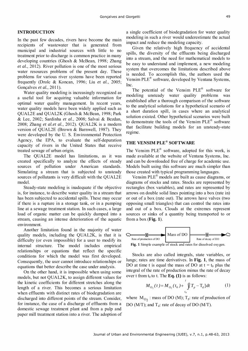
Gonçalves and Giorgetti
Journal of Urban and Environmental Engineering (JUEE), v.7, n.1, p.48-63, 2013
49
INTRODUCTION
In the past few decades, rivers have become the main recipients of wastewater that is generated from municipal and industrial sources with little to no treatment prior to discharge is common practice in many developing countries (Ghosh & McBean, 1998; Zhang et al., 2012). River pollution is one of the most serious water resources problems of the present day. These problems for various river systems have been reported frequently (Drolc & Koncan, 1996; Liu et al., 2005; Gonçalves et al., 2011).
Water quality modeling is increasingly recognized as a useful tool for acquiring valuable information for optimal water quality management. In recent years, water quality models have been widely applied such as QUAL2E and QUAL2K (Ghosh & McBean, 1998; Park & Lee, 2002; Sardinha et al., 2008; Salvai & Bezdan, 2008; Zhang et al.et al., 2012). QUAL2K is a modern version of QUAL2E (Brown & Barnwell, 1987). They were developed by the U. S. Environmental Protection Agency, the EPA, to evaluate the self-depuration capacity of rivers in the United States that receive treated sewage of urban origin.
The QUAL2E model has limitations, as it was created specifically to analyze the effects of steady sources of pollution under American standards. Simulating a stream that is subjected to unsteady sources of pollutants is very difficult with the QUAL2E model.
Steady-state modeling is inadequate if the objective is, for instance, to describe water quality in a stream that has been subjected to accidental spills. These may occur if there is a rupture in a storage tank, or in a pumping line at a sewage treatment station. In such cases, a large load of organic matter can be quickly dumped into a stream, causing an intense deterioration of the aquatic environment.
Another limitation found in the majority of water quality models, including the QUAL2K, is that it is difficulty (or even impossible) for a user to modify its internal structure. The model includes empirical relationships or equations that reflect the specific conditions for which the model was first developed. Consequently, the user cannot introduce relationships or equations that better describe the case under analysis.
On the other hand, it is impossible when using some models, but not QUAL2K, to assign different values for the kinetic coefficients for different stretches along the length of a river. This becomes a serious limitation when effluents with distinct rates of biodegradation are discharged into different points of the stream. Consider, for instance, the case of a discharge of effluents from a domestic sewage treatment plant and from a pulp and paper mill treatment station into a river. The adoption of
a single coefficient of biodegradation for water quality modeling in such a river would underestimate the actual impact and reduce the modeling capacity.
Given the relatively high frequency of accidental spills, the diversity of the effluents being discharged into a stream, and the need for mathematical models to be easy to understand and implement, a new modeling system that overcomes the limitations described above is needed. To accomplish this, the authors used the Vensim PLE® software, developed by Ventana Systems, Inc.
The potential of the Vensim PLE® software for modeling unsteady water quality problems was established after a thorough comparison of the software to the analytical solutions for a hypothetical scenario of a short duration spill, in cases where an analytical solution existed. Other hypothetical scenarios were built to demonstrate the tools of the Vensim PLE® software that facilitate building models for an unsteady-state regime. THE VENSIM PLE® SOFTWARE
The Vensim PLE® software, adopted for this work, is made available at the website of Ventana Systems, Inc. and can be downloaded free of charge for academic use. Models built using this software are much simpler than those created with typical programming languages.
Vensim PLE® models are built as cause diagrams, or diagrams of stocks and rates. Stocks are represented by rectangles (box variables), and rates are represented by arrows on double solid lines pointing into a box (rate in) or out of a box (rate out). The arrows have valves (two opposing small triangles) that can control the rates into and out of a box. Clouds at the extremes represent sources or sinks of a quantity being transported to or from a box (Fig. 1).
Fig. 1 Simple example of stock and rates for dissolved oxygen. Stocks are also called integrals, state variables, or
lungs; rates are time derivatives. In Fig. 1, the mass of DO at time t is equal the mass of DO at t = t0 plus the integral of the rate of production minus the rate of decay over t from t0 to t. The Eq. (1) is as follows:
dtT[)t(M)t(Mt
t
pOO ∫0
22]Td0 (1)
where 2OM : mass of DO (M); Tp: rate of production of
DO (M/T); and Td: rate of decay of DO (M/T).
Gonçalves and Giorgetti
Journal of Urban and Environmental Engineering (JUEE), v.7, n.1, p.48-63, 2013
50
The Vensim PLE® software offers two alternatives for numerical integration, namely Euler’s method and the fourth order Runge-Kutta method (RK4).
BUILDING THE MODEL FOR A WATER COLUMN
The development of a water quality model involves building two sub-systems, one for the hydraulics of the water body (balance of volume), and another describing causes for the changes in concentration of the water quality variables, namely, the chemical, physical and biological processes, and the transport mechanisms represented by advection, diffusion and dispersion.
When building a model, a river channel is divided into control volumes (CV) of length Δx, each one comprising two sub-systems as described in the preceding paragraph.
To balance volume at steady-state conditions, the flow rate out of the CV equals the sum of the flow rates into the CV (flow rate from the upstream CV plus flow rate from sources of pollution) minus the flow rate of the water sinks (pumping stations). This equation is:
iCs,ifp,1-ii QQQQ
(2)
where Qi: flow rate out of CV i and flow rate into downstream CV i+1 (L3/T); Qi-1: flow rate into CV i and flow rate out of upstream CV i+1 (L3/T); Qfp,i: flow rate from sources of pollution into CV i (L3/T); and Qcs,i: flow rate of water pumped out of i (L3/T).
The term Qfp,i is also used to represent the flow rate from a tributary of the river that can be modeled if necessary.
The differential equation resulting from the balance of volume used for modeling with Vensim PLE® is shown below:
iCs,ifp,1-ii QQQQdt
dV (3)
The combination of Eqs (2) and (3) gives dV/dt=0.
Therefore, V, the volume of the CV, does not vary with time.
To simulate an accidental pollutant discharge (unsteady perturbations) we assume that the flow rate of the pollutant is negligible when compared to the flow rate of the river. Therefore, the flow rate of the accidental pollutant is not considered in the balance of volume; the flow rate out is equal to the flow rate in.
This simplification limits use of the simulation only when unsteady accidental discharges do not lead to drastic increases in the river flow rate. Therefore, before any simulation can begin, the ratios between the flow
rates of these perturbation discharges and the river’s flow rate have to be critically examined.
According to Chapra et al. (2003), there are three ways to determine a river’s mean flow velocity - namely weirs, rating curves, and using Manning’s formula. For this work, we chose to use the most common alternative given by Eq. (4), Manning’s formula. However, it is very easy to substitute this with another formulation as follows:
21
o3
2
h IRn
1=U (4)
where U: cross-sectional average velocity (L/T); n: roughness coefficient (T/L1/3); Rh: hydraulic radius (L); and Io: longitudinal bottom slope (L/L).
For a simpler representation of the mass balance, we assume one-dimensional water flow, for which the concentration of any variable remains constant across each flow section. The resulting partial differential equation derived from the mass balance is as follows:
V
W
V
S
x ∂
C ∂AD
x ∂
∂
A
1
x ∂
(QC) ∂
A
1
t ∂
C ∂tL
tt
)(
(5)
where S: sources or sinks (M/T); C: concentration of a variable (M/L3); At: area of the flow section (L2); DL: longitudinal dispersion coefficient (L2/T); and W: sources of pollution or sinks of pumping water (M/T).
The term S, sources or sinks, represents the contribution of the physical, chemical, and/or biological processes responsible for the production and/or consumption of the mass of the variables under simulation. All of the processes modeled are shown in Table 1.
To simulate water temperature, a thermal energy balance is calculated for control volume. This energy balance is very similar to the mass balance stated above.
For the thermal (internal) energy balance, both in and out flows of energy are considered. They are associated with the temperatures of the pollutant discharges, linked to the outflow of energy connected to water pumping, and linked to sources and sinks of other forms of energy exchange between the water and the environment.
The third part is modeled upon the combination of five processes: 1. Short wave solar radiation; 2. Long wave atmospheric radiation; 3. Short wave radiation emitted by the water; 4. Air-water convection; and 5. Evaporation-condensation. Processes 1 and 2 are modeled as sources of thermal energy; process 3 is modeled as a sink of thermal energy; processes 4 and 5 represent either sources or sinks, depending upon the sign of the temperature difference (water minus air
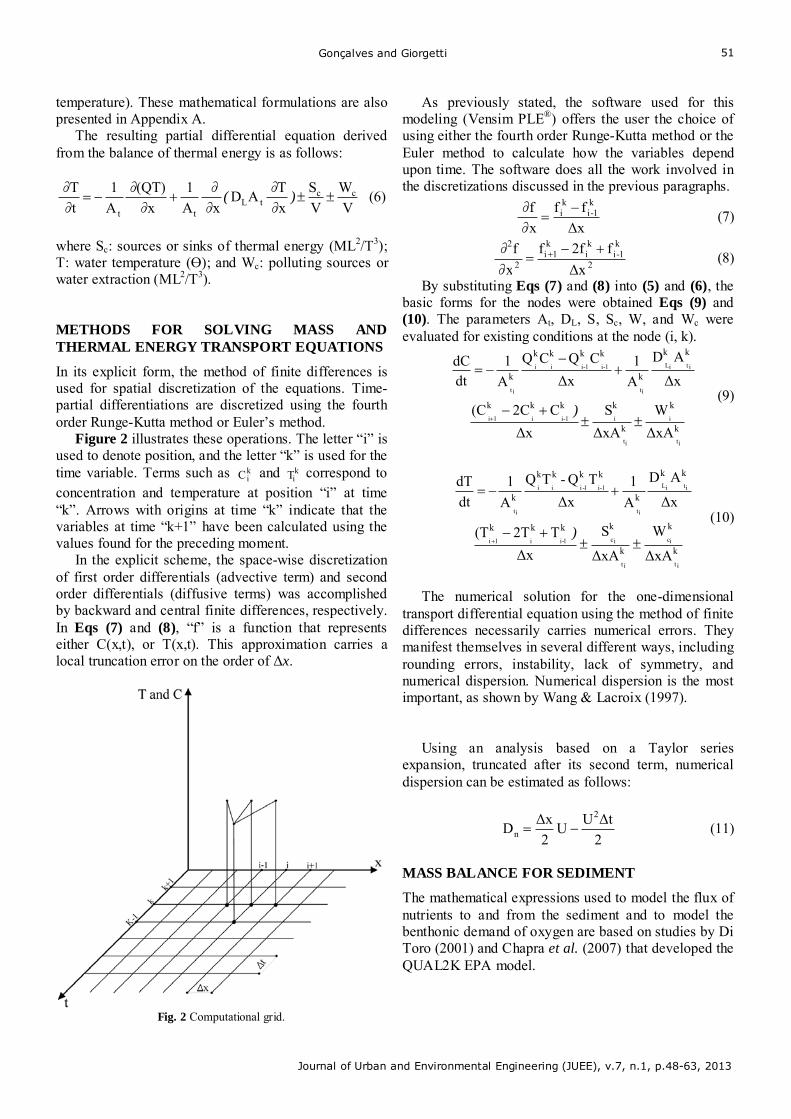
Gonçalves and Giorgetti
Journal of Urban and Environmental Engineering (JUEE), v.7, n.1, p.48-63, 2013
51
temperature). These mathematical formulations are also presented in Appendix A.
The resulting partial differential equation derived from the balance of thermal energy is as follows:
V
W
V
S
x ∂
T ∂AD
x ∂
∂
A
1
x ∂
(QT) ∂
A
1
t ∂
T ∂ cctL
tt
)(
(6)
where Sc: sources or sinks of thermal energy (ML2/T3); T: water temperature (Ө); and Wc: polluting sources or water extraction (ML2/T3). METHODS FOR SOLVING MASS AND THERMAL ENERGY TRANSPORT EQUATIONS
In its explicit form, the method of finite differences is used for spatial discretization of the equations. Time-partial differentiations are discretized using the fourth order Runge-Kutta method or Euler’s method.
Figure 2 illustrates these operations. The letter “i” is used to denote position, and the letter “k” is used for the time variable. Terms such as k
iC and kiT correspond to
concentration and temperature at position “i” at time “k”. Arrows with origins at time “k” indicate that the variables at time “k+1” have been calculated using the values found for the preceding moment.
In the explicit scheme, the space-wise discretization of first order differentials (advective term) and second order differentials (diffusive terms) was accomplished by backward and central finite differences, respectively. In Eqs (7) and (8), “f” is a function that represents either C(x,t), or T(x,t). This approximation carries a local truncation error on the order of Δx.
Fig. 2 Computational grid.
As previously stated, the software used for this modeling (Vensim PLE®) offers the user the choice of using either the fourth order Runge-Kutta method or the Euler method to calculate how the variables depend upon time. The software does all the work involved in the discretizations discussed in the previous paragraphs.
Δx
ff
x ∂
f ∂ k1-i
ki
(7)
2
k1-i
ki
k1i
2
2
Δx
f2ff
x ∂
f∂
(8)
By substituting Eqs (7) and (8) into (5) and (6), the basic forms for the nodes were obtained Eqs (9) and (10). The parameters At, DL, S, Sc, W, and Wc were evaluated for existing conditions at the node (i, k).
k
k
k
kkkk
kk
k
kkkk
k
it
i
it
i1-ii1i
itiL
it
1-i1-iii
it
ΔxA
W
ΔxA
S
Δx
C2C(C
Δx
AD
A
1Δx
CQCQ
A
1dtdC
)
(9)
k
k
k
kkkk
kk
k
kkkk
k
it
ic
it
ic1-ii1i
itiL
it
1-i1-iii
it
ΔxA
W
ΔxA
S
Δx
T2T(T
Δx
AD
A
1
Δx
TQ-TQ
A
1
dt
dT
)
(10)
The numerical solution for the one-dimensional
transport differential equation using the method of finite differences necessarily carries numerical errors. They manifest themselves in several different ways, including rounding errors, instability, lack of symmetry, and numerical dispersion. Numerical dispersion is the most important, as shown by Wang & Lacroix (1997).
Using an analysis based on a Taylor series expansion, truncated after its second term, numerical dispersion can be estimated as follows:
2
ΔtUU
2
ΔxD
2
n
(11)
MASS BALANCE FOR SEDIMENT
The mathematical expressions used to model the flux of nutrients to and from the sediment and to model the benthonic demand of oxygen are based on studies by Di Toro (2001) and Chapra et al. (2007) that developed the QUAL2K EPA model.
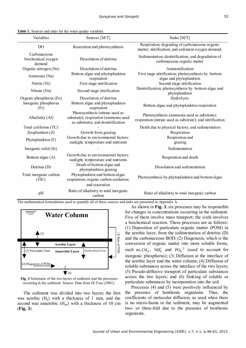
Gonçalves and Giorgetti
Journal of Urban and Environmental Engineering (JUEE), v.7, n.1, p.48-63, 2013
52
Table 1. Sources and sinks for the water quality variables
Variables Sources [M/T] Sinks [M/T]
DO Reaeration and photosynthesis Respiration; degrading of carbonaceous organic matter; nitrification; and sediment oxygen demand.
Carbonaceous biochemical oxygen
demand Dissolution of detritus
Sedimentation; denitrification; and degradation of carbonaceous organic matter
Organic nitrogen (No) Dissolution of detritus Ammonification
Ammonia (Na) Bottom algae and phytoplankton respiration
First stage nitrification; photosynthesis by bottom algae and phytoplankton
Nitrite (Ni) First stage nitrification Second stage nitrification
Nitrate (Nn) Second stage nitrification Denitrification; photosynthesis by bottom algae and phytoplankton
Organic phosphorus (Fo) Dissolution of detritus Hydrolysis Inorganic phosphorus
(Fi) Bottom algae and phytoplankton
respiration Bottom algae and phytoplankton respiration
Alkalinity (Al) Photosynthesis (nitrate used as
substrate); respiration (ammonia used as substrate); and denitrification
Photosynthesis (ammonia used as substrate); respiration (nitrate used as substrate); and nitrification
Total coliforms (TC) - Death due to physical factors; and sedimentation Zooplankton (Z) Growth from grazing Respiration
Phytoplankton (F) Growth due to environmental factors: sunlight, temperature and nutrients
Respiration and grazing
Inorganic solid (Si) - Sedimentation
Bottom algae (A) Growth due to environmental factors: sunlight, temperature and nutrients
Respiration and death
Detritus (D) Death of bottom algae and phytoplankton grazing
Dissolution and sedimentation
Total inorganic carbon (TIC)
Phytoplankton and bottom algae respiration; organic carbon oxidation; Photosynthesis by phytoplankton and bottom algae
and reaeration
pH Ratio of alkalinity to total inorganic carbon
Ratio of alkalinity to total inorganic carbon
The mathematical formulations used to quantify all of these sources and sinks are presented in Appendix A.
Fig. 3 Schematic of the two layers of sediment and the processes
occurring in the sediment. Source: Data from Di Toro (2001).
The sediment was divided into two layers; the first was aerobic (Ha) with a thickness of 1 mm, and the second was anaerobic (Han) with a thickness of 10 cm (Fig. 3).
As shown in Fig. 3, six processes may be responsible for changes in concentrations occurring in the sediment. Five of them involve mass transport; the sixth involves a biochemical reaction. These processes are as follows: (1) Deposition of particulate organic matter (POM) in the aerobic layer, from the sedimentation of detritus (D) and the carbonaceous BOD; (2) Diagenesis, which is the conversion of organic matter into more soluble forms, such as, 4CH , +
4NH and 3-4PO (used to account for
inorganic phosphorus); (3) Diffusion at the interface of the aerobic layer and the water column; (4) Diffusion of soluble substances across the interface of the two layers; (5) Pseudo-diffusive transport of particulate substances across the two layers; and (6) Sinking of soluble or particulate substances by incorporation into the soil.
Processes (4) and (5) were positively influenced by the presence of benthonic organisms. Thus, the coefficients of molecular diffusion, as used when there is no micro-fauna in the sediment, may be augmented two- or three-fold due to the presence of benthonic organisms.
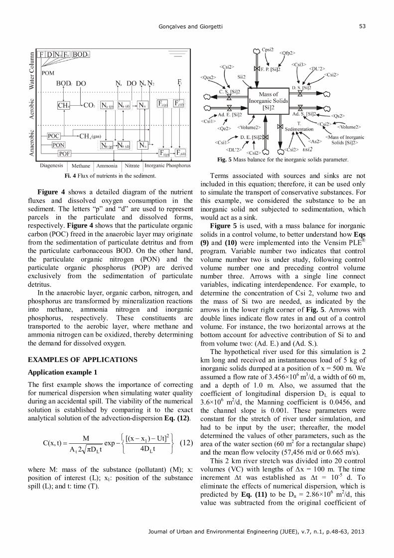
Gonçalves and Giorgetti
Journal of Urban and Environmental Engineering (JUEE), v.7, n.1, p.48-63, 2013
53
Fi. 4 Flux of nutrients in the sediment.
Figure 4 shows a detailed diagram of the nutrient
fluxes and dissolved oxygen consumption in the sediment. The letters “p” and “d” are used to represent parcels in the particulate and dissolved forms, respectively. Figure 4 shows that the particulate organic carbon (POC) freed in the anaerobic layer may originate from the sedimentation of particulate detritus and from the particulate carbonaceous BOD. On the other hand, the particulate organic nitrogen (PON) and the particulate organic phosphorus (POP) are derived exclusively from the sedimentation of particulate detritus.
In the anaerobic layer, organic carbon, nitrogen, and phosphorus are transformed by mineralization reactions into methane, ammonia nitrogen and inorganic phosphorus, respectively. These constituents are transported to the aerobic layer, where methane and ammonia nitrogen can be oxidized, thereby determining the demand for dissolved oxygen. EXAMPLES OF APPLICATIONS
Application example 1
The first example shows the importance of correcting for numerical dispersion when simulating water quality during an accidental spill. The viability of the numerical solution is established by comparing it to the exact analytical solution of the advection-dispersion Eq. (12).
t4D
Ut])x[(xexp
tπD2A
Mt)C(x,
L
21
Lt
(12)
where M: mass of the substance (pollutant) (M); x: position of interest (L); x1: position of the substance spill (L); and t: time (T).
Fig. 5 Mass balance for the inorganic solids parameter.
Terms associated with sources and sinks are not
included in this equation; therefore, it can be used only to simulate the transport of conservative substances. For this example, we considered the substance to be an inorganic solid not subjected to sedimentation, which would act as a sink.
Figure 5 is used, with a mass balance for inorganic solids in a control volume, to better understand how Eqs (9) and (10) were implemented into the Vensim PLE®
program. Variable number two indicates that control volume number two is under study, following control volume number one and preceding control volume number three. Arrows with a single line connect variables, indicating interdependence. For example, to determine the concentration of Csi 2, volume two and the mass of Si two are needed, as indicated by the arrows in the lower right corner of Fig. 5. Arrows with double lines indicate flow rates in and out of a control volume. For instance, the two horizontal arrows at the bottom account for advective contribution of Si to and from volume two: (Ad. E.) and (Ad. S.).
The hypothetical river used for this simulation is 2 km long and received an instantaneous load of 5 kg of inorganic solids dumped at a position of x = 500 m. We assumed a flow rate of 3.456×10⁶ m3/d, a width of 60 m, and a depth of 1.0 m. Also, we assumed that the coefficient of longitudinal dispersion DL is equal to 3.6×10⁶ m2/d, the Manning coefficient is 0.0456, and the channel slope is 0.001. These parameters were constant for the stretch of river under simulation, and had to be input by the user; thereafter, the model determined the values of other parameters, such as the area of the water section (60 m2 for a rectangular shape) and the mean flow velocity (57,456 m/d or 0.665 m/s).
This 2 km river stretch was divided into 20 control volumes (VC) with lengths of ∆x = 100 m. The time increment ∆t was established as ∆t = 10-5 d. To eliminate the effects of numerical dispersion, which is predicted by Eq. (11) to be Dn = 2.86×10⁶ m2/d, this value was subtracted from the original coefficient of
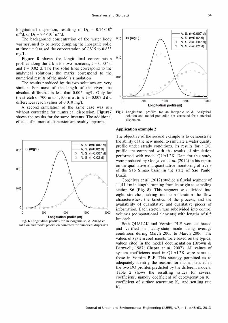
Gonçalves and Giorgetti
Journal of Urban and Environmental Engineering (JUEE), v.7, n.1, p.48-63, 2013
54
longitudinal dispersion, resulting in DL = 0.74×10⁶ m2/d, or DL = 7.4×10⁷ m2/d.
The background concentration of the water body was assumed to be zero; dumping the inorganic solid at time t = 0 raised the concentration of CV 5 to 0.833 mg/L.
Figure 6 shows the longitudinal concentration profiles along the 2 km for two moments, t = 0.007 d and t = 0.02 d. The two solid lines correspond to the analytical solutions; the marks correspond to the numerical results of the model’s simulation.
The results produced by the two solutions are very similar. For most of the length of the river, the absolute difference is less than 0.005 mg/L. Only for the stretch of 700 m to 1,100 m at time t = 0.007 d did differences reach values of 0.010 mg/L.
A second simulation of the same case was run without correcting for numerical dispersion. Figure7 shows the results for the same instants. The additional effects of numerical dispersion are readily apparent.
Fig. 6 Longitudinal profiles for an inorganic solid. Analytical
solution and model prediction corrected for numerical dispersion.
Fig.7 Longitudinal profiles for an inorganic solid. Analytical
solution and model prediction not corrected for numerical dispersion.
Application example 2
The objective of the second example is to demonstrate the ability of the new model to simulate a water quality profile under steady conditions. Its results for a DO profile are compared with the results of simulation performed with model QUAL2K. Data for this study were produced by Gonçalves et al. (2012) in his report on the qualitative and quantitative monitoring of rivers of the São Simão basin in the state of São Paulo, Brazil.
Gonçalves et al. (2012) studied a fluvial segment of 11,41 km in length, running from its origin to sampling station S6 (Fig. 8). This segment was divided into eight stretches, taking into consideration the flow characteristics, the kinetics of the process, and the availability of quantitative and qualitative pieces of information. Each stretch was subdivided into control volumes (computational elements) with lengths of 0.5 km each.
Both QUAL2K and Vensim PLE were calibrated and verified in steady-state mode using average conditions during March 2005 to March 2006. The values of system coefficients were based on the typical values cited in the model documentation (Brown & Barnwell, 1987; Chapra et al. 2007). All values of system coefficients used in QUAL2K were same as those in Vensim PLE. This strategy permitted us to adequately identify the reasons for inconsistencies in the two DO profiles predicted by the different models. Table 2 shows the resulting values for several coefficiens, namely coefficient of deoxygenation Kd, coefficient of surface reaeration K2, and settling rate Ks.
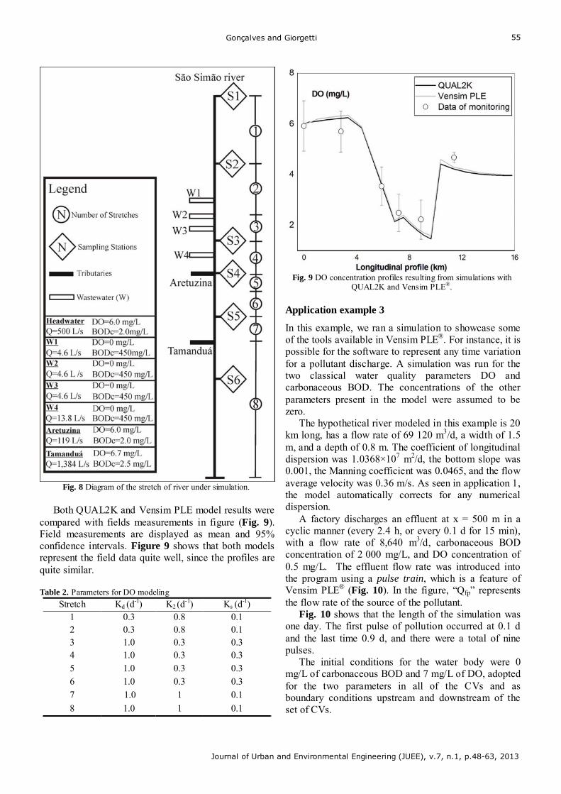
Gonçalves and Giorgetti
Journal of Urban and Environmental Engineering (JUEE), v.7, n.1, p.48-63, 2013
55
Fig. 8 Diagram of the stretch of river under simulation.
Both QUAL2K and Vensim PLE model results were
compared with fields measurements in figure (Fig. 9). Field measurements are displayed as mean and 95% confidence intervals. Figure 9 shows that both models represent the field data quite well, since the profiles are quite similar. Table 2. Parameters for DO modeling
Stretch Kd (d-1) K2 (d
-1) Ks (d-1)
1 0.3 0.8 0.1 2 0.3 0.8 0.1 3 1.0 0.3 0.3 4 1.0 0.3 0.3 5 1.0 0.3 0.3 6 1.0 0.3 0.3 7 1.0 1 0.1
8 1.0 1 0.1
Fig. 9 DO concentration profiles resulting from simulations with
QUAL2K and Vensim PLE®.
Application example 3
In this example, we ran a simulation to showcase some of the tools available in Vensim PLE®. For instance, it is possible for the software to represent any time variation for a pollutant discharge. A simulation was run for the two classical water quality parameters DO and carbonaceous BOD. The concentrations of the other parameters present in the model were assumed to be zero.
The hypothetical river modeled in this example is 20 km long, has a flow rate of 69 120 m3/d, a width of 1.5 m, and a depth of 0.8 m. The coefficient of longitudinal dispersion was 1.0368×10⁷ m2/d, the bottom slope was 0.001, the Manning coefficient was 0.0465, and the flow average velocity was 0.36 m/s. As seen in application 1, the model automatically corrects for any numerical dispersion.
A factory discharges an effluent at x = 500 m in a cyclic manner (every 2.4 h, or every 0.1 d for 15 min), with a flow rate of 8,640 m3/d, carbonaceous BOD concentration of 2 000 mg/L, and DO concentration of 0.5 mg/L. The effluent flow rate was introduced into the program using a pulse train, which is a feature of Vensim PLE® (Fig. 10). In the figure, “Qfp” represents the flow rate of the source of the pollutant.
Fig. 10 shows that the length of the simulation was one day. The first pulse of pollution occurred at 0.1 d and the last time 0.9 d, and there were a total of nine pulses.
The initial conditions for the water body were 0 mg/L of carbonaceous BOD and 7 mg/L of DO, adopted for the two parameters in all of the CVs and as boundary conditions upstream and downstream of the set of CVs.
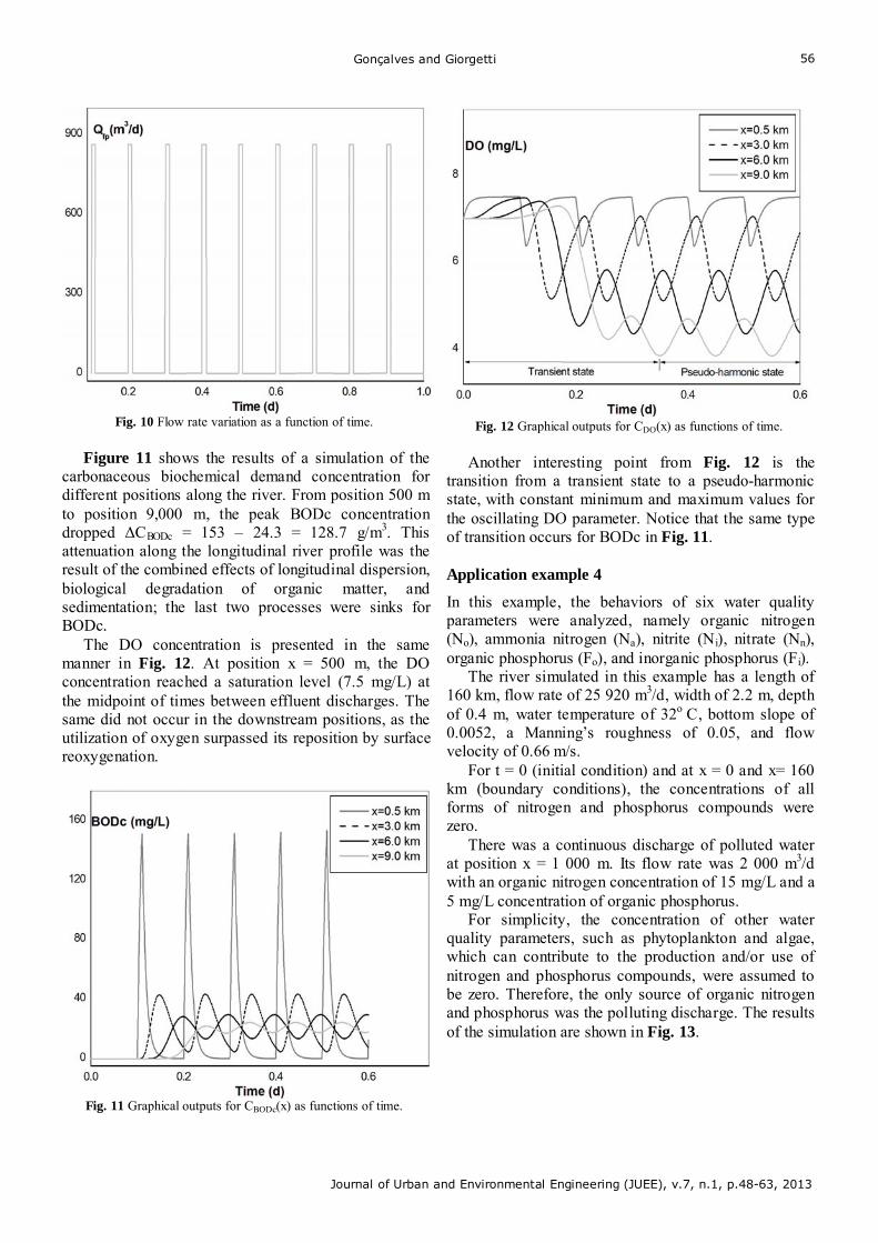
Gonçalves and Giorgetti
Journal of Urban and Environmental Engineering (JUEE), v.7, n.1, p.48-63, 2013
56
Fig. 10 Flow rate variation as a function of time.
Figure 11 shows the results of a simulation of the
carbonaceous biochemical demand concentration for different positions along the river. From position 500 m to position 9,000 m, the peak BODc concentration dropped ΔCBODc = 153 – 24.3 = 128.7 g/m3. This attenuation along the longitudinal river profile was the result of the combined effects of longitudinal dispersion, biological degradation of organic matter, and sedimentation; the last two processes were sinks for BODc.
The DO concentration is presented in the same manner in Fig. 12. At position x = 500 m, the DO concentration reached a saturation level (7.5 mg/L) at the midpoint of times between effluent discharges. The same did not occur in the downstream positions, as the utilization of oxygen surpassed its reposition by surface reoxygenation.
Fig. 11 Graphical outputs for CBODc(x) as functions of time.
Fig. 12 Graphical outputs for CDO(x) as functions of time.
Another interesting point from Fig. 12 is the
transition from a transient state to a pseudo-harmonic state, with constant minimum and maximum values for the oscillating DO parameter. Notice that the same type of transition occurs for BODc in Fig. 11. Application example 4
In this example, the behaviors of six water quality parameters were analyzed, namely organic nitrogen (No), ammonia nitrogen (Na), nitrite (Ni), nitrate (Nn), organic phosphorus (Fo), and inorganic phosphorus (Fi).
The river simulated in this example has a length of 160 km, flow rate of 25 920 m3/d, width of 2.2 m, depth of 0.4 m, water temperature of 32o C, bottom slope of 0.0052, a Manning’s roughness of 0.05, and flow velocity of 0.66 m/s.
For t = 0 (initial condition) and at x = 0 and x= 160 km (boundary conditions), the concentrations of all forms of nitrogen and phosphorus compounds were zero.
There was a continuous discharge of polluted water at position x = 1 000 m. Its flow rate was 2 000 m3/d with an organic nitrogen concentration of 15 mg/L and a 5 mg/L concentration of organic phosphorus.
For simplicity, the concentration of other water quality parameters, such as phytoplankton and algae, which can contribute to the production and/or use of nitrogen and phosphorus compounds, were assumed to be zero. Therefore, the only source of organic nitrogen and phosphorus was the polluting discharge. The results of the simulation are shown in Fig. 13.
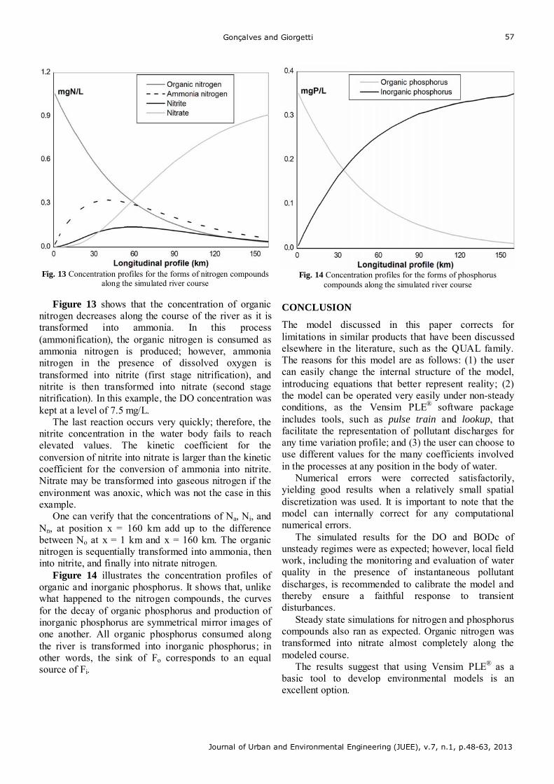
Gonçalves and Giorgetti
Journal of Urban and Environmental Engineering (JUEE), v.7, n.1, p.48-63, 2013
57
Fig. 13 Concentration profiles for the forms of nitrogen compounds
along the simulated river course
Figure 13 shows that the concentration of organic nitrogen decreases along the course of the river as it is transformed into ammonia. In this process (ammonification), the organic nitrogen is consumed as ammonia nitrogen is produced; however, ammonia nitrogen in the presence of dissolved oxygen is transformed into nitrite (first stage nitrification), and nitrite is then transformed into nitrate (second stage nitrification). In this example, the DO concentration was kept at a level of 7.5 mg/L.
The last reaction occurs very quickly; therefore, the nitrite concentration in the water body fails to reach elevated values. The kinetic coefficient for the conversion of nitrite into nitrate is larger than the kinetic coefficient for the conversion of ammonia into nitrite. Nitrate may be transformed into gaseous nitrogen if the environment was anoxic, which was not the case in this example.
One can verify that the concentrations of Na, Ni, and Nn, at position x = 160 km add up to the difference between No at x = 1 km and x = 160 km. The organic nitrogen is sequentially transformed into ammonia, then into nitrite, and finally into nitrate nitrogen.
Figure 14 illustrates the concentration profiles of organic and inorganic phosphorus. It shows that, unlike what happened to the nitrogen compounds, the curves for the decay of organic phosphorus and production of inorganic phosphorus are symmetrical mirror images of one another. All organic phosphorus consumed along the river is transformed into inorganic phosphorus; in other words, the sink of Fo corresponds to an equal source of Fi.
Fig. 14 Concentration profiles for the forms of phosphorus
compounds along the simulated river course
CONCLUSION
The model discussed in this paper corrects for limitations in similar products that have been discussed elsewhere in the literature, such as the QUAL family. The reasons for this model are as follows: (1) the user can easily change the internal structure of the model, introducing equations that better represent reality; (2) the model can be operated very easily under non-steady conditions, as the Vensim PLE® software package includes tools, such as pulse train and lookup, that facilitate the representation of pollutant discharges for any time variation profile; and (3) the user can choose to use different values for the many coefficients involved in the processes at any position in the body of water.
Numerical errors were corrected satisfactorily, yielding good results when a relatively small spatial discretization was used. It is important to note that the model can internally correct for any computational numerical errors.
The simulated results for the DO and BODc of unsteady regimes were as expected; however, local field work, including the monitoring and evaluation of water quality in the presence of instantaneous pollutant discharges, is recommended to calibrate the model and thereby ensure a faithful response to transient disturbances.
Steady state simulations for nitrogen and phosphorus compounds also ran as expected. Organic nitrogen was transformed into nitrate almost completely along the modeled course.
The results suggest that using Vensim PLE® as a basic tool to develop environmental models is an excellent option.
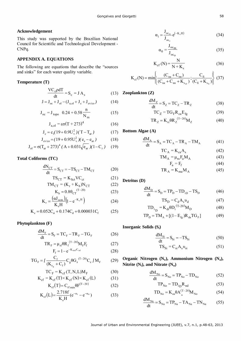
Gonçalves and Giorgetti
Journal of Urban and Environmental Engineering (JUEE), v.7, n.1, p.48-63, 2013
58
Acknowledgement
This study was supported by the Brazilian National Council for Scientific and Technological Development - CNPq.
APPENDIX A. EQUATIONS
The following are equations that describe the “sources and sinks” for each water quality variable. Temperature (T)
sce AJ=S=dt
ρdTVC (13)
)ev/cocola,oloc JJJ(JJJ (14)
N
n0.58+0.24J=J
mtopooc (15)
( )4ola, 273+Tεσ=J (16)
)()( ar2v1c TT0.9U19cJ (17)
)()( ars2vev/co ee0.95U19J (18)
))(( rar4
arol C1e0.031A273)σ(TJ (19)
Total Coliforms (TC)
CTCTCTCT TMTSS
dt
dN (20)
ctSctCT VCK=TS (21)
CTbrCT )NK+(K=TM (22) 20)(T
CTb 0.8θK (23)
HK
e
ocmr
ee1HK
αJK (24)
fdsie 0.000031C0.174C0.052CK (25)
Phytoplankton (F)
FFFFF TGTRTCS
dt
dM (26)
fF20T
frfF FMθRμTR (27) odresf CK
f e1F (28)
Fz20)(T
zgfs
fF MCθGC
)C(K
CTG
g
][
(29)
FcfF L)MN,T,(K=TC (30) ( ) ( ) ( )LK×NK×TK=K cfcfcfcf (31) 20T
máxrfcf θFCTK (32)
)e(eHK
2.718fLK 01 αα
ecf
(33)
HK
oc
oc1
e
o
m eJ
Jα (34)
ooc
moc0 J
J=α (35)
scf K+N
N=(N)K (36)
)K(C
C;
)KC(C
)C(Cmin(N)K
finf sfi
fi
snnna
nnnacf (37)
Zooplankton (Z)
ZZZZ TRTCS
dt
dM (38)
fgcaFZ ERTG=TC (39)
Z
20TZrzZ MθRKTR (40)
Bottom Algae (A)
AAAAA TMTRTCS
dt
dM (41)
scaA AK=TC (42)
AaraA MFμ=TM (43)
fa F=F (44) AmaA MK=TR (45)
Detritus (D)
DDiDDD TSTDTPS
dt
dM (46)
dsdD υAC=TS (47)
( )D
20-TidiDi MθDK=TD (48)
]TG)RE[(1TMTP FdafgAD (49)
Inorganic Solids (Si)
SiSiSi TSS
dt
dM (50)
sissiSi υAC=TS (51)
Organic Nitrogen (No), Ammonium Nitrogen (Na), Nitrite (Ni), and Nitrate (Nn)
NoNoNoNo TDTPS
dt
dM (52)
ndDiNo RTD=TP (53)
No
20ToaNo MθAKTD
m
(54)
NaNaNaNaNa TNTATPS
dt
dM (55)
Gonçalves and Giorgetti
Journal of Urban and Environmental Engineering (JUEE), v.7, n.1, p.48-63, 2013
59
)TR(R+)TR(R+TD=TP FnaAndNoNa (56)
)TCR+TCR(F=TA AndFnaamNa (57)
)C+C)(C+Kp(
KpC+
)C+Kp)(C+Kp(
CC=F
nnnannna
nana
nnnanana
nnnaam
(58)
NaiNa
20TaiNa FMθNKTN (59)
odiniCKNai e1F (60)
NiNaNi
Ni TNTNSdt
dM (61)
NiiNi
20TinNi FMθNKTN (62)
odinnCKNii e1F (63)
NnesNnNiNnNn TD-TA-TN=S=
dt
dM (64)
)F(1MθNKTD desNn20T
desNnes (65)
)e(11F odides CKdes
(66) ))(( AndFnaamNn TCRTCRF1TA (67)
Organic (Fo) and Inorganic (Fi) Phosphorous
FoFoFoFo TDTPS
dt
dM (68)
pdDiFo RTD=TP (69)
Fo
20ToiFo MθHKTD
fo
(70)
FiFiFiFi TATPS
dt
dM (71)
)TR(R+)TR(R+TD=TP FpaApdFoFi (72) )TCR+TCR(=TA ApdFpaFi (73)
Carbonaceous Biochemical Demand (BODc)
DBOcDBOcDes
DBOcDeDBOcDBOcDBOc
TSTD
TDTPSdt
dM
(74)
occdDiDBOc RRTD=TP (75)
DBOciDBOc20T
dDBOce FMθDKTD (76)
odidegr
c
CKiDBO e1F (77)
H
Ui+K=K 1d (78)
ondesNnesDBOces RTD=TD (79)
DBOc
20TDBOcDBOcDBOc MθSKsTS (80)
Dissolved Oxygen (DO)
ODesoOD
ODODeODODOD
TNTD
TRTRTFSdt
dM
(81)
)VC(CθRKTR odS20T
e2ODe (82)
AlgaeBottom
occdA
tonPhytoplank
occaFOD )RRTR(+)RRTR(=TR (83)
iDBODBOc
20TdDBOceODeso c
FMθDKTDTD (84)
onnNioniNaOD RTN+RTN=TN (85)
AlgaeBottom
occdA
tonPhytoplank
occaFOD )RRTC(+)RRTC(=TF (86)
Total Inorganic Carbon (TIC)
CITeCIT
COeCITCITCIT
TFTD
TRTRSdt
dM2
(87)
)VFCs(CKTR ocitCOCOCOe 222 (88)
Cmol,coDBOceCITe RRTD=TD (89)
AlgaeBottom
Cmol,cdA
tonPhytoplank
Cmol,caFCIT )RRTR(+)RRTR(=TR (90)
AlgaeBottom
Cmol,cdA
tonPhytoplank
Cmol,caFCIT )RRTR(+)RRTR(=TF (91)
Alkalinity (Al.)
Al.iAl.Al.esAl.Al.Al. TNTDTDTAS
dt
dN (92)
AlgaeBottom
Cmol,cdAam
tonPhytoplank
Cmol,caFam
AlgaeBottom
Cmol,cdAam
tonPhytoplank
Cmol,caFamAl.
nn],R[HRRTCF1
nn],R[HRRTCF1
na],R[HRRTRF
na],R[HRRTRFTA
)(
)(
)(
)(
(93)
AlgaeBottom
Cmol,cdAam
tonPhytoplank
Cmol,caFam
AlgaeBottom
Cmol,cdAam
tonPhytoplank
Cmol,caFamAl.
nn],R[HRRTRF1
nn],R[HRRTRF1
na],R[HRRTCF
na],R[HRRTCFTD
)(
)(
)(
)(
(94)
des],R[HRTD=TD +Nmol,NnesAl.es (95)
Gonçalves and Giorgetti
Journal of Urban and Environmental Engineering (JUEE), v.7, n.1, p.48-63, 2013
60
( ) nitri],R[HRTN+TN=TN +Nmol,NiNaAl.i (96)
pH
(97)
APPENDIX B. NOMENCLATURE
A: coefficient related to air temperature and to the actual solar radiation and clean sky solar radiation; range: 0.5 to 0.7 (non-dimensional) A 0.7 for air temperatures of above 20o C.
A0: coefficient for the beginning of the curve (non-dimensional). A1: coefficient for the middle of the curve (non-dimensional). A2: coefficient for the end of the curve (non-dimensional). As: surface area for each control volume (cm2).
c1: Bowen’s coefficient (mm Hg/oC). Cal.: concentration of calcium carbonate (mgCaCO3/L). Cct: concentration of total coliforms (Norg/L). Ccit: concentration of total inorganic carbon (mol/L). CCO2s: saturation concentration of CO2 in water (mol/L). Cd: concentration of detritus (mgD/L). Ce: specific heat (cal/goC). Cf: concentration of phytoplankton (mgA/L).
Cfi: concentration of inorganic phosphorus (mgP/L). Cg: kinetic coefficient for zooplankton grazing (L/mgCd). Cna: concentration of ammonium nitrogen (mgN/L). Cnn: concentration of nitrate (mgN/L). Cod: concentration of dissolved oxygen (mgO/L). Cr: coefficient of reflection (non-dimensional). Crfmáx: coefficient for the maximum growth of phytoplankton ( 1.8); this value varies as a function of the phytoplankton species (1/d). Cs: saturation concentration of dissolved oxygen (mgO/L). Csi: concentration of inorganic solids (mg/L). Cz: concentration of zooplankton (mgC/L).
ear: vapor pressure in the atmosphere (mm Hg). Efg: efficiency factor for grazing (non-dimensional).
: emissivity of water ( 0.97) (non-dimensional). es: water vapor pressure (mm Hg). f: photoperiod (non-dimensional). Fa: factor of attenuation for bottom algae respiration (non-dimensional). Fam: factor of preference for ammonium (non-dimensional). FDBOci: factor of correction (attenuation) of the coefficient of deoxygenation as a function of DO concentration (non-dimensional). Fdes: factor of correction (attenuation) of the coefficient of denitrification as a function of DO concentration (non-dimensional). Ff: factor of correction (attenuation) of the coefficient of phytoplankton respiration as a function of DO concentration (non-dimensional). FNai: factor of correction (attenuation) for the coefficient of first stage nitrification as a function of DO concentration (non-dimensional). FNii: factor of correction (attenuation) for the coefficient of second stage nitrification as a function of DO concentration (non-dimensional). Fo: fraction of free inorganic carbon [non-dimensional] H: river depth (m). Ha0: initial value 1.05 (non-dimensional). HaLim: limiting value for growth; function of temperature (non-dimensional). i: coefficient of activity in the bottom mud (non-dimensional). Ja,ol: short wave radiation flux emitted by the water (cal/cm2 d). Jc: convective flux of thermal energy between the water and the atmosphere (cal/cm2 d). Jev/co: flux of thermal energy eliminated from the water by evaporation, or gained by condensation (cal/cm2 d).
Joc: flux of short wave solar radiation (cal/cm2 d). Jocm: average short wave solar radiation flux (cal/cm2 d). Joco: optimal short wave solar radiation flux for phytoplankton growth (300 cal/cm2 d). Jol: flux of long wave radiation from the atmosphere (cal/cm2 d). Jtopo: flux of solar radiation at the upper layers of the atmosphere (cal/m2 d), calculated as Io senα; Io is the solar constant, equal to 2.88×10⁷ cal m2/d; α is the inclination of solar rays to the horizontal. K CO2: coefficient of global transfer of CO2 (1/d). K: growth coefficient (≈27) (non-dimensional). K1: kinetic coefficient for deoxygenation (1/d). K2: coefficient of surface reoxygenation (1/d). Kai: kinetic coefficient for conversion of ammonia into nitrite (1/d). Kb: coefficient for coliform death as function of temperature, salinity, and predation (1/d).
)A-C
CK
0
0Lim
Lim
)A-C
CK
0
0Lim
Lim
)A-C
CK(
0
0Lim
Lim
cit
al.
2cit
al.
1cit
al.
0cit
al.
eHa
HaHa1
Ha
eHa
HaHa1
Ha
eHa
HaHa1
Ha
1)C
C27.5pHa
(
(
(
Gonçalves and Giorgetti
Journal of Urban and Environmental Engineering (JUEE), v.7, n.1, p.48-63, 2013
61
Kca: coefficient for the (flux of) growth of bottom algae (gD/m2 d). Kcf (L): coefficient for the effect of solar light on phytoplankton growth (non-dimensional).
Kcf (N): coefficient for the effect of nutrients on phytoplankton growth (non-dimensional).
Kcf (T): coefficient for the effect of temperature on phytoplankton growth (1/d).
Kd: coefficient of effective deoxygenation in the river (1/d). Kdi: kinetic coefficient for the dissolution of detritus; normally in the range 0.3 to 0.7 (1/d). Kdes: kinetic coefficient for denitrification (1/d). Ke: coefficient of solar light extinction (1/m).
Kidegr: coefficient of inhibition of deoxygenation by low DO concentration (L/mgO). Kides: coefficient of inhibition of denitrification (L/mgO). Kin: kinetic coefficient for conversion of nitrite into nitrate (1/d). Kini: coefficient of inhibition of first stage nitrification by low DO concentration (L/mgO). Kini: coefficient of inhibition of first stage nitrification by low DO concentration (L/mgO). Kma: death rate of bottom algae (1/d). Koa: kinetic coefficient for conversion of organic nitrogen into ammonium (1/d). Koi: kinetic coefficient for conversion of organic phosphorus into orthophosphate (1/d). Kpna: coefficient for preference of bottom algae and phytoplankton for ammonium (mgN/L). Kr: rate of decay of TC due to solar radiation (1/d). Kresf: coefficient of inhibition of breathing due to low e DO concentration (L/mgO). Krz: kinetic coefficient for the respiration of phytoplankton; normally in the range 0.01 to 0.05 (1/d). Ks: constant of half saturation (mg/L). KSct: first order sedimentation coefficient (1/d). KsDBOc: sedimentation coefficient for the BODc (1/d). KSff: constant of half saturation for inorganic phosphorous; normally in the range 0.001 to 0.005 (mgP/L). KSg: constant of half saturation for zooplankton grazing (mgA/L). KSnf: constant of half saturation for nitrogen; normally in the range 0.01 to 0.02 (mgN/L). KSfi: constant of half saturation for phosphorus (mgP/L). MA: mass of bottom algae (mgD). MCIT: inorganic total carbon (mol). MD: mass of detritus (mgD). MDBOc: mass of BODc (mgO). MF: mass of phytoplankton (mgA).
MFi: mass of inorganic phosphorus (mgP). MFo: mass of organic phosphorus (mgP).
MNa: mass of ammonium nitrogen (mgN). MNa: mass of nitrite (mgN). MNn: mass of nitrate (mgN). MNo: mass of organic nitrogen (mgN). MOD: mass of dissolved oxygen (mgO). MSi: mass of inorganic solids (mg). MZ: mass of zooplankton (mgC). n: effective daily duration of solar radiation (h). Nm: maximum daily duration of solar radiation (h). N: nutrient concentration (mg/L). NAl.: number of hydrogen gram equivalent ions (eqH+). NCT: number of total coliforms (Norg). pHa: pH variation caused by autochtonous processes (non-dimensional). R[H+],des: hydrogen gram equivalent ions per nitrogen mol consumed during denitrification (eqH+/molN). R[H+],na: hydrogen ions freed or consumed per mol of carbon when ammonium nitrogen is used as substratum (eqH+/molC) R[H+],nitri: gram equivalent hydrogen ions freed per mol of nitrified nitrogen (eqH+/molN). R[H+],nn: hydrogen ions freed or consumed per mol of carbon when nitrate is used as substratum (eqH+/molC). Rca: carbon generated per unit of mass of a-chlorophyll (non-dimensional). Rcd: mass of organic carbon liberated per mass of detritus dissolved in the water (non-dimensional). Rco: mass of oxidized carbon per mass of consumed oxygen (non-dimensional). Rda: stoichiometric ratio between detritus and a-chlorophyll used to express the mass of phytoplankton (non-dimensional). Rmol,C: constant to transform mass of carbon into mols (molC/g). Rmol,N: constant to transform mass of nitrogen into mols (molN/g). Rna: mass of nitrogen liberated per mass of a-chlorophyll dissolved in the water (non-dimensional). Rnd: mass of nitrogen liberated per mass of detritus dissolved in the water (non-dimensional). Roc: mass of consumed oxygen per mass of decomposed carbon (non-dimensional). Rondes: mass of non-used carbon per mass of denitrified nitrate (non-dimensional). Roni: mass of consumed oxygen per mass of oxidized ammonium (non-dimensional). Ronn: mass of consumed oxygen per mass of oxidized nitrite (non-dimensional). Rpa: coefficient for conversion of a-chlorophyll into phosphorous (non-dimensional). Rpd: mass of organic phosphorous liberated per mass of detritus dissolved in the water (non-dimensional). T : water temperature (o C) TAAl.: rate of alkalinity increase caused by the aquatic vegetable community (eqH+/d).
Gonçalves and Giorgetti
Journal of Urban and Environmental Engineering (JUEE), v.7, n.1, p.48-63, 2013
62
TAFi: rate of inorganic phosphorus assimilation by phytoplankton and bottom algae (mgP/d). TANa: rate of ammonium assimilation by phytoplankton and bottom algae (mgN/d). TANn: rate of nitrate assimilation by phytoplankton and bottom algae (mgN/d). Tar: air temperature (o C). TCA: rate of growth of bottom algae (mgD/d). TCF: rate of growth of bottom phytoplankton (mgA/d). TCZ: rate of growth of bottom zooplankton (mgC/d). TDAl.: rate of alkalinity decay caused by the aquatic vegetable community (eqH+/d). TDeCIT: rate of increase of total inorganic carbon due to oxidation of organic carbon (mol/d). TDeDBOc: rate of degradation of organic carbon (mgO/d). TDesAl.: rate of increase of alkalinity due to denitrification (eqH+/d). TDesDBOc: rate of decay of BODc due to denitrification (mgO/d). TDesNn: rate of denitrification (mgN/d). TDesOD: rate of deoxygenation caused by the degradation of organic carbon (mgO/d). TDFo: rate of decay of organic phosphorus (mgP/d). TDiD: rate of dissolution of detritus (mgD/d). TDNo rate of decay of organic nitrogen (mgN/d). TFCIT: rate of decay of total inorganic carbon due to photosynthesis of phytoplankton and bottom algae (mol/d). TFOD: rate of increase dissolved oxygen due to photosynthesis (mgO/d). TGF: rate of zooplankton grazing (mgA/d). TMA: rate of death of bottom algae (mgD/d). TMCT: rate of death of total coliforms (Norg/d). TNiAl.: rate of decay of alkalinity due to nitrification (eqH+/d). TNNa: rate of first stage nitrification (mgN/d). TNNi: rate of second stage nitrification (mgN/d). TNOD: rate of DO loss due to nitrification (mgO/d). TPD:rate of production of detritus (mgD/d). TPDBOc: rate of production of BODc (mgO/d). TPFo: rate of production of organic phosphorus (mgP/d). TPNa: rate of production of ammonium nitrogen (mgN/d). TPNo rate of production of organic nitrogen (mgN/d). TRA: rate of respiration of bottom (mgD/d). TRCIT: rate of increase of inorganic carbon due to respiration of phytoplankton and bottom algae (mol/d). TReCO2: rate of CO2 transfer between water and atmosphere (mol/d). TReOD: rate of surface superficial reoxygenation (gO/d). TRF: rate of phytoplankton respiration (mgA/d). TROD: rate of decrease of DO due to respiration by phytoplankton and bottom algae (mgO/d). TRZ: rate of phytoplankton respiration (mgC/d).
TSCT: rate of sedimentation of total coliforms (Norg/d). TSD: rate of sedimentation of detritus (mgD/d). TSDBOc: rate of sedimentation of BDOc (mgO/d). TSsi: rate of sedimentation of inorganic solids (mg/L). Uv: wind speed (m/s). α: proportionality constant ( 1) (non-dimensional). θAm: coefficient of the effect of temperature on ammonification (non-dimensional). θCT: coefficient of the effect of temperature on mortality (non-dimensional). θDi: coefficient of the effect of temperature on the dissolution of detritus (non-dimensional). θF: coefficient of the effect of temperature on the growth of phytoplankton (non-dimensional). θGz: coefficient of the effect of temperature on zooplankton grazing (non-dimensional). θHfo: coefficient of the effect of temperature on organic phosphorus hydrolysis (non-dimensional). θN: coefficient of the effect of temperature on nitrification (non-dimensional). θRe: coefficient of the effect of temperature on surface reoxygenation (non-dimensional). θRf: coefficient of the effect of temperature on phytoplankton respiration (non-dimensional). θRz: coefficient of the effect of temperature on zooplankton respiration (non-dimensional). θSDBOc: coefficient of the effect of temperature on sedimentation of BDOc (non-dimensional). μra: rate of respiration of bottom algae (1/d).
μrf: kinetic coefficient for the respiration of phytoplankton (1/d). σ: Stefan-Boltzmann constant (cal/cm2 d K4). υd: apparent settling speed for detritus (m/d). υsi: apparent settling speed for inorganic solids (m/d).
REFERENCES
Brown L. C. & Barnwell T, O. (1987) The enhanced stream water quality models QUAL2E and QUAL2E-UNCAS: Documentation and user manual. Environmental Research Laboratory, Office of Research and Development. U.S. EPA/600/3-87 /007.
Chapra S. C. & Pelletier G. J. (2003) QUAL2K: A modeling framework for simulating river and stream water quality: documentation and user manual. Civil and Environmental Engineering Dept., Tufts University, Medford.
Chapra S. C., Pelletier G. J. & Tao H. (2007) QUAL2K: A modeling framework for simulating river and stream water quality: documentation and user manual. Version 2.07. Civil and Environmental Engineering Dept., Tufts University, Medford.
Di Toro, D. M. (2001) Sediment Flux Modeling. Wiley-Interscience, New York, USA.
Drolc, A. & Koncan, J. Z. (1996) Water quality modeling of the river sava, Slovenia. Wat. Res. 30(11), 2587–2592.
Ghosh, N. C. & Mcbean, E. A. (1998) Water quality modeling of the Kali river, India. Water, Air, and Soil Pollution. 102, 91-103.
Gonçalves, J. C. S. I., Sardinha, D. S. & Boesso, F. F. (2011) Modelo numérico para a simulação da qualidade da água no trecho urbano do rio Jaú, Município de Jaú-SP. Revista de Estudos Ambientais. 13(2), 44-56.

Gonçalves and Giorgetti
Journal of Urban and Environmental Engineering (JUEE), v.7, n.1, p.48-63, 2013
63
Gonçalves, J. C. S. I., Sardinha, D. S., Souza, A. D. G., Dibiazi, A. L. B., Godoy, L. H. & Conceição, F. T. (2012) Avaliação espaço-temporal da qualidade da água e simulação de autodepuração na bacia hidrográfica do córrego São Simão-SP. Revista Ambiente & Água. 7(3), 141-154.
Liu, W.C., Liu, S. Y., Hsu, M. S. & Kuo, A. Y. (2005) Water quality modeling to determine minimum instream flow for fish survival in tidal rivers. Journal of Environmental Management. 52, 55–66.
Park, S. S. & Lee, Y. S. A water quality modeling study of the Nakdong river, Korea. Ecological Modelling. 152, 65-75.
Salvai, A. & Bezdan, A. (2008) Water quality model QUAL2K in TMDL development. Balwois Ohrid, Republic of Macedonia. 27, 1-8.
Sardinha, D. S., Conceição, F. T., Souza, A. D. G., Silveira, A., de Júlio, M. & Gonçalves, J. C. S. I. (2008) Avaliação da qualidade da água e autodepuração do Ribeirão do Meio, Leme (SP). Engenharia Sanitária e Ambiental. 13(3), 329-338.
Wang, H. Q. & Lacroix, M. (1997) Optimal weighting in the finite difference solution of the convection-dispersion equation. Journal of Hydrology. 200, 228-242.
Zhang, R., Qian, X., Li, H., Yuan, X. & Ye, R. (2012) Selection of optimal river water quality improvement programs using Qual2K: A case study of Taihu Lake Basin, China. Science of the Total Environment. 431, 278-285.
Fracassia and Lollo
Journal of Urban and Environmental Engineering (JUEE), v.7, n.1, p. 64-73, 2013
64
Journal of Urban and Environmental Engineering, v.7, n.1, p. 64-73
Journal of Urban and Environmental Engineering
UEEJ ISSN 1982-3932
doi: 10.4090/ juee.2013.v7n1.064073 www.journal-uee.org
URBAN SPRAWL IN SMALL CITIES, ANALYSIS OF THE MUNICIPALITY OF SÃO PEDRO (SP): POTENTIALS AND
CONSTRAINS
Priscila C. Fracassi1, José A. de Lollo2 1Urban Engineering Post-graduation Program, Federal University of São Carlos, Brazil
2Department of Civil Engineering, Univ. Estadual Paulista (UNESP) at Ilha Solteira, Brazil
Received 5 July 2012; received in revised form 30 January 2013; accepted 28 March 2013
Abstract: Urban sprawl in small cities has led to the occupation of unsuitable areas, resulting in
peripheralization and in the occupation of fragile environments. In these occupations, the physical characteristics of the environment are often disrespected. In this context, the present article reports on a case study in the municipality of São Pedro, state of São Paulo, Brazil, which presents and discuss a set of natural factors (geological and geomorphological) conditioning the occurrence of erosion and gravitational mass movements, which are limiting factors for urban sprawl. The methodology employed in this study was based on field work, bibliographic research, and data collection, analysis and GIS-based systematization, which allowed for a spatial reading of the urban sprawl to indicate, from different perspectives, how the phenomenon is manifested. Thus, it was possible to draw up a chart highlighting the areas with the greatest potential for occupation and those with restrictions due to their greater susceptibility to erosion and mass movements. The main identified natural factors of restriction were steepness and soil conditions and law enforced restrictions (environmental protection areas).
Keywords:
Urban sprawl; small cities; fragile environments; landslides; erosion; GIS
© 2013 Journal of Urban and Environmental Engineering (JUEE). All rights reserved.
Correspondence to: José A. de Lollo, Tel.: +55 18 3743 1215; Fax: +55 18 3743 1160. E-mail: [email protected]
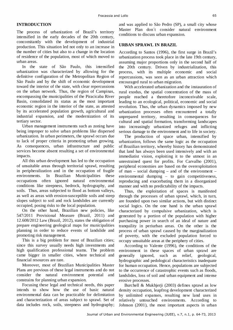
Fracassia and Lollo
Journal of Urban and Environmental Engineering (JUEE), v.7, n.1, p. 64-73, 2013
65
INTRODUCTION
The process of urbanization of Brazil’s territory intensified in the early decades of the 20th century, concomitantly with the development of industrial production. This situation led not only to an increase in the number of cities but also to a change in the location of residence of the population, most of which moved to urban areas.
In the state of São Paulo, this intensified urbanization was characterized by allowing for the definitive configuration of the Metropolitan Region of São Paulo and by the shift of economic development toward the interior of the state, with clear repercussions on the urban network. Thus, the region of Campinas, encompassing the municipalities of the Piracicaba River Basin, consolidated its status as the most important economic region in the interior of the state, as attested by its accelerated population growth, agricultural and industrial expansion, and the modernization of its tertiary sector.
Urban management instruments such as zoning have being improper to solve urban problems like dispersed urbanization. In urban perimeters, the sprawl occurs due to lack of proper criteria in promoting urban growing. As consequences, urban infrastructure and public services become absent resulting a set of environmental impacts.
All this urban development has led to the occupation of unsuitable areas through territorial sprawl, resulting in peripheralization and in the occupation of fragile environments. In Brazilian Municipalities these occupations often ignored natural environmental conditions like steepness, bedrock, hydrography, and soils. Thus, areas subjected to flood as bottom valleys, as well as areas with erosion-susceptible soils and steep slopes subject to soil and rock landslides are currently occupied, posing risks to the local population.
On the other hand, Brazilian new policies, like 547/2011 Provisional Measure (Brazil, 2011) and 12.608/2012 Law (Brazil, 2012), states the obligation of prepare engineering geological maps for municipalities planning in order to reduce events of landslide and promoting risk management.
This is a big problem for most of Brazilian cities; since this survey usually needs high investments and high qualification professional teams. The problem came bigger in smaller cities, where technical and financial resources are rare.
Moreover, most of Brazilian Municipalities Master Plans are previous of these legal instruments and do not consider the natural environment potential and constrains for planning urban expansion.
Focusing these legal and technical needs, this paper intends to show how the use of basic natural environmental data can be practicable for delimitation and characterization of areas subject to sprawl. Set of data includes rock, soils, steepness and hydrography;
and was applied to São Pedro (SP), a small city whose Master Plan don´t consider natural environment conditions to discuss urban expansion. URBAN SPRAWL IN BRAZIL
According to Santos (1996), the first surge in Brazil’s urbanization process took place in the late 19th century, assuming major proportions only in the second half of the 20th century. Driven by industrialization, this process, with its multiple economic and social repercussions, was seen as an urban attraction which encouraged rural to urban migration.
With accelerated urbanization and the instauration of rural exodus, the spatial concentration of the mass of people reached a theretofore inconceivable scale, leading to an ecological, political, economic and social revolution. Thus, the urban dynamics imposed by new urbanization processes often encountered a totally unprepared territory, resulting in consequences for cultural and spatial formation, transforming landscapes into increasingly urbanized refuges and inflicting serious damage to the environment and to life in society.
The production of space urban, intensified by urbanization, follows the same logic as the occupation of Brazilian territory, whereby history has demonstrated that land has always been used intensively and with an immediatist vision, exploiting it to the utmost in an unrestrained quest for profits. For Carvalho (2001), peripheral economies are based on the overexploitation of man – social dumping – and of the environment – environmental dumping – to gain competitiveness, reproducing and exacerbating them in a disorganized manner and with no predictability of the impacts.
Thus, the exploitation of spaces is manifested through the processes of urban sprawl, which, in turn, are founded upon two similar actions, but with distinct social logics. On the one hand is the urban sprawl characterized by compulsive urbanization, which is generated by a portion of the population with higher purchasing power in search of an ideal of nature and tranquility in periurban areas. On the other is the process of urban sprawl caused by the marginalization of poverty, with the excluded population forced to occupy unsuitable areas at the periphery of cities.
According to Valente (1996), the conditions of the environment in these spaces of urban sprawl are generally ignored, such as relief, geological, hydrographic and pedological characteristics inadequate for human occupation. Hence, populations are subjected to the occurrence of catastrophic events such as floods, landslides, loss of soil and urban equipment and intense erosive processes.
Burchell & Mukhjerji (2003) defines sprawl as low density occupation, leapfrog development characterized by unlimited expanses, resulting new land uses in relatively untouched environments. According to Johnson (2001), the most important aspects in urban
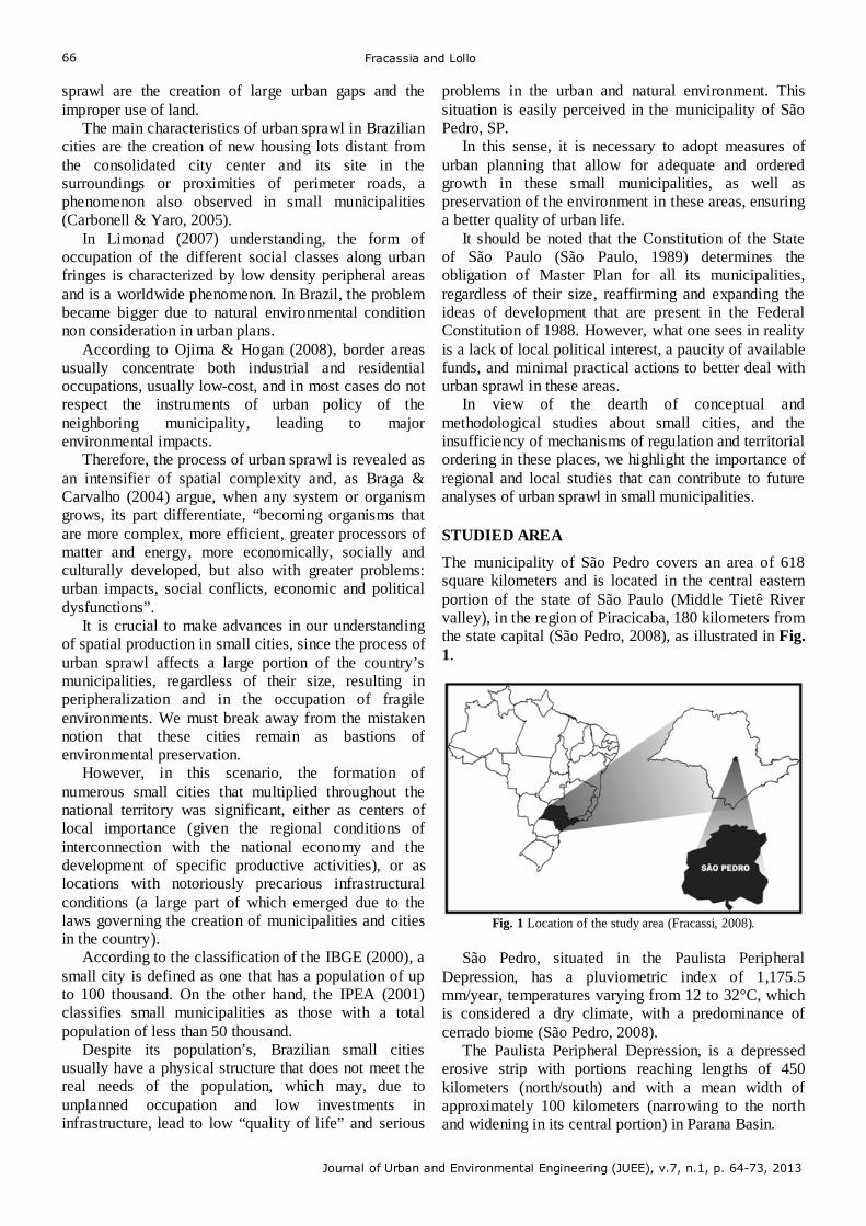
Fracassia and Lollo
Journal of Urban and Environmental Engineering (JUEE), v.7, n.1, p. 64-73, 2013
66
sprawl are the creation of large urban gaps and the improper use of land.
The main characteristics of urban sprawl in Brazilian cities are the creation of new housing lots distant from the consolidated city center and its site in the surroundings or proximities of perimeter roads, a phenomenon also observed in small municipalities (Carbonell & Yaro, 2005).
In Limonad (2007) understanding, the form of occupation of the different social classes along urban fringes is characterized by low density peripheral areas and is a worldwide phenomenon. In Brazil, the problem became bigger due to natural environmental condition non consideration in urban plans.
According to Ojima & Hogan (2008), border areas usually concentrate both industrial and residential occupations, usually low-cost, and in most cases do not respect the instruments of urban policy of the neighboring municipality, leading to major environmental impacts.
Therefore, the process of urban sprawl is revealed as an intensifier of spatial complexity and, as Braga & Carvalho (2004) argue, when any system or organism grows, its part differentiate, “becoming organisms that are more complex, more efficient, greater processors of matter and energy, more economically, socially and culturally developed, but also with greater problems: urban impacts, social conflicts, economic and political dysfunctions”.
It is crucial to make advances in our understanding of spatial production in small cities, since the process of urban sprawl affects a large portion of the country’s municipalities, regardless of their size, resulting in peripheralization and in the occupation of fragile environments. We must break away from the mistaken notion that these cities remain as bastions of environmental preservation.
However, in this scenario, the formation of numerous small cities that multiplied throughout the national territory was significant, either as centers of local importance (given the regional conditions of interconnection with the national economy and the development of specific productive activities), or as locations with notoriously precarious infrastructural conditions (a large part of which emerged due to the laws governing the creation of municipalities and cities in the country).
According to the classification of the IBGE (2000), a small city is defined as one that has a population of up to 100 thousand. On the other hand, the IPEA (2001) classifies small municipalities as those with a total population of less than 50 thousand.
Despite its population’s, Brazilian small cities usually have a physical structure that does not meet the real needs of the population, which may, due to unplanned occupation and low investments in infrastructure, lead to low “quality of life” and serious
problems in the urban and natural environment. This situation is easily perceived in the municipality of São Pedro, SP.
In this sense, it is necessary to adopt measures of urban planning that allow for adequate and ordered growth in these small municipalities, as well as preservation of the environment in these areas, ensuring a better quality of urban life.
It should be noted that the Constitution of the State of São Paulo (São Paulo, 1989) determines the obligation of Master Plan for all its municipalities, regardless of their size, reaffirming and expanding the ideas of development that are present in the Federal Constitution of 1988. However, what one sees in reality is a lack of local political interest, a paucity of available funds, and minimal practical actions to better deal with urban sprawl in these areas.
In view of the dearth of conceptual and methodological studies about small cities, and the insufficiency of mechanisms of regulation and territorial ordering in these places, we highlight the importance of regional and local studies that can contribute to future analyses of urban sprawl in small municipalities. STUDIED AREA
The municipality of São Pedro covers an area of 618 square kilometers and is located in the central eastern portion of the state of São Paulo (Middle Tietê River valley), in the region of Piracicaba, 180 kilometers from the state capital (São Pedro, 2008), as illustrated in Fig. 1.
Fig. 1 Location of the study area (Fracassi, 2008).
São Pedro, situated in the Paulista Peripheral
Depression, has a pluviometric index of 1,175.5 mm/year, temperatures varying from 12 to 32°C, which is considered a dry climate, with a predominance of cerrado biome (São Pedro, 2008).
The Paulista Peripheral Depression, is a depressed erosive strip with portions reaching lengths of 450 kilometers (north/south) and with a mean width of approximately 100 kilometers (narrowing to the north and widening in its central portion) in Parana Basin.
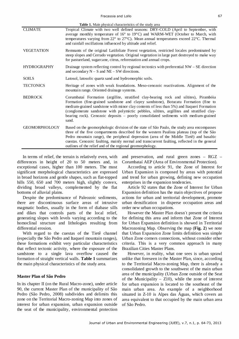
Fracassia and Lollo
Journal of Urban and Environmental Engineering (JUEE), v.7, n.1, p. 64-73, 2013
67
Table 1. Main physical characteristics of the study area
CLIMATE Tropical Climate with two well defined seasons: DRY-COLD (April to September, with average monthly temperature of 16° to 19°C) and WARM-WET (October to March, with temperatures varying from 22° to 27°C). Mean annual temperatures exceed 22°C. Thermal and rainfall oscillations influenced by altitude and relief.
VEGETATION Remnants of the original Latifoliate Forest vegetation, restricted locales predominated by steep slopes and Cerrado vegetation. Original vegetation in large part destroyed to make way for pastureland, sugarcane, citrus, reforestation and annual crops.
HYDROGRAPHY Drainage system reflecting control by regional tectonics with preferential NW – SE direction and secondary N – S and NE – SW directions.
SOILS Latosol, latosolic quartz sand and hydromorphic soils.
TECTONICS Heritage of zones with weak foundations. Meso-cenozoic reactivations. Alignment of the mountain range. Oriented drainage systems.
BEDROCK Corumbataí Formation (argillite, stratified clay-bearing rock and siltites), Pirambóia Formation (fine-grained sandstone and clayey sandstone), Botucatu Formation (fine to medium-grained sandstone with minor clay contents of less than 5%) and Itaquerí Formation (conglomerate sandstone with polymictic pebbles, siltites, argillites and stratified clay-bearing rock). Cenozoic deposits – poorly consolidated sediments with medium-grained sand.
GEOMORPHOLOGY Based on the geomorphologic division of the state of São Paulo, the study area encompasses three of the five compartments described for the western Paulista plateau (top of the São Pedro mountain range), the peripheral depression (area of the Middle Tietê) and basaltic cuestas. Cenozoic faulting, mainly normal and transcurrent faulting, reflected in the general outlines of the relief and of the regional geomorphology.
In terms of relief, the terrain is relatively even, with
differences in height of 20 to 50 meters and, in exceptional cases, higher than 100 meters. The most significant morphological characteristics are expressed in broad horizons and gentle shapes, such as flat-topped hills 550, 650 and 700 meters high, slightly convex, dividing broad valleys, complemented by the flat bottoms of alluvial plains.
Despite the predominance of Paleozoic sediments, there are discontinuous surface areas of intrusive magmatic bodies, usually in the form of diabase sills and dikes that controls parts of the local relief, generating slopes with levels varying according to the homoclinal structure and lithologies resulting from differential erosion.
With regard to the cuestas of the Tietê channel (especially the São Pedro and Itaquerí mountain ranges), these formations exhibit very particular characteristics that reflect tectonic activity, where the exposure of the sandstone to a single lava overflow caused the formation of straight vertical walls. Table 1 summarizes the main physical characteristics of the study area.
Master Plan of São Pedro
In its chapter II (on the Rural Macro-zone), under article 90, the current Master Plan of the municipality of São Pedro (São Pedro, 2008) subdivides and delimits this zone on the Territorial Macro-zoning Map into zones of interest for urban expansion, urban expansion outside the seat of the municipality, environmental protection
and preservation, and rural green zones – RGZ – Corumbataí AEP (Area of Environmental Protection).
According to article 91, the Zone of Interest for Urban Expansion is composed by areas with potential and trend for urban growing, defining new occupation enterprises in the expansion tendencies.
Article 92 states that the Zone of Interest for Urban Expansion definition has the main objectives of propose actions for urban and territorial development, promote urban densification in disperse occupation areas and order new urban occupations.
However the Master Plan doesn´t present the criteria for defining this area and inform that Zone of Interest for Urban Expansion definition is showed in Territorial Macrozoning Map. Observing the map (Fig. 2) we note that Urban Expansion Zone limits definition was simple Urban Zone corners connections, without consider other criteria. This is a very common approach in many Brazilian Cities Master Plans.
However, in reality, what one sees is urban sprawl unlike that foreseen in the Master Plan, since, according to the Territorial Macro-zoning Map, there is already a consolidated growth to the southwest of the main urban area of the municipality (Urban Zone outside of the Seat of the Municipality – Z10), while the zone of interest for urban expansion is located to the southeast of the main urban area. An example of a neighborhood situated in Z-10 is Alpes das Águas, which covers an area equivalent to that occupied by the main urban area of São Pedro.
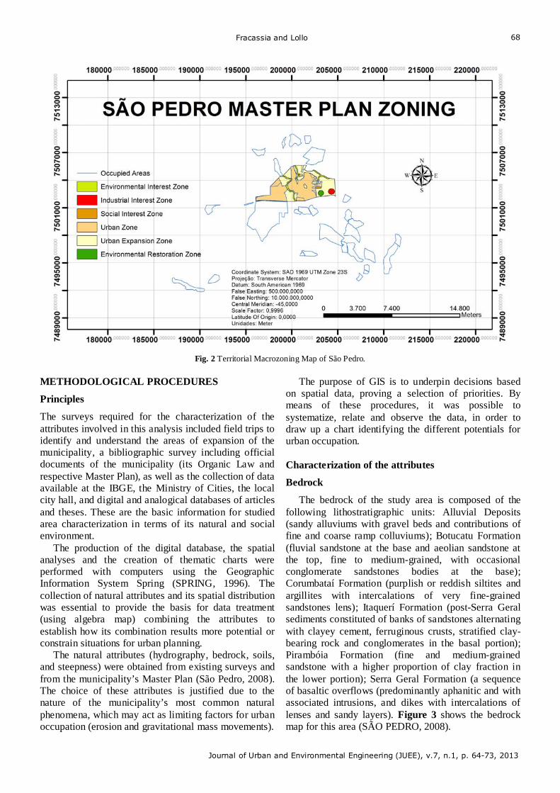
Fracassia and Lollo
Journal of Urban and Environmental Engineering (JUEE), v.7, n.1, p. 64-73, 2013
68
Fig. 2 Territorial Macrozoning Map of São Pedro.
METHODOLOGICAL PROCEDURES
Principles
The surveys required for the characterization of the attributes involved in this analysis included field trips to identify and understand the areas of expansion of the municipality, a bibliographic survey including official documents of the municipality (its Organic Law and respective Master Plan), as well as the collection of data available at the IBGE, the Ministry of Cities, the local city hall, and digital and analogical databases of articles and theses. These are the basic information for studied area characterization in terms of its natural and social environment.
The production of the digital database, the spatial analyses and the creation of thematic charts were performed with computers using the Geographic Information System Spring (SPRING, 1996). The collection of natural attributes and its spatial distribution was essential to provide the basis for data treatment (using algebra map) combining the attributes to establish how its combination results more potential or constrain situations for urban planning.
The natural attributes (hydrography, bedrock, soils, and steepness) were obtained from existing surveys and from the municipality’s Master Plan (São Pedro, 2008). The choice of these attributes is justified due to the nature of the municipality’s most common natural phenomena, which may act as limiting factors for urban occupation (erosion and gravitational mass movements).
The purpose of GIS is to underpin decisions based on spatial data, proving a selection of priorities. By means of these procedures, it was possible to systematize, relate and observe the data, in order to draw up a chart identifying the different potentials for urban occupation. Characterization of the attributes
Bedrock
The bedrock of the study area is composed of the following lithostratigraphic units: Alluvial Deposits (sandy alluviums with gravel beds and contributions of fine and coarse ramp colluviums); Botucatu Formation (fluvial sandstone at the base and aeolian sandstone at the top, fine to medium-grained, with occasional conglomerate sandstones bodies at the base); Corumbataí Formation (purplish or reddish siltites and argillites with intercalations of very fine-grained sandstones lens); Itaquerí Formation (post-Serra Geral sediments constituted of banks of sandstones alternating with clayey cement, ferruginous crusts, stratified clay-bearing rock and conglomerates in the basal portion); Pirambóia Formation (fine and medium-grained sandstone with a higher proportion of clay fraction in the lower portion); Serra Geral Formation (a sequence of basaltic overflows (predominantly aphanitic and with associated intrusions, and dikes with intercalations of lenses and sandy layers). Figure 3 shows the bedrock map for this area (SÃO PEDRO, 2008).
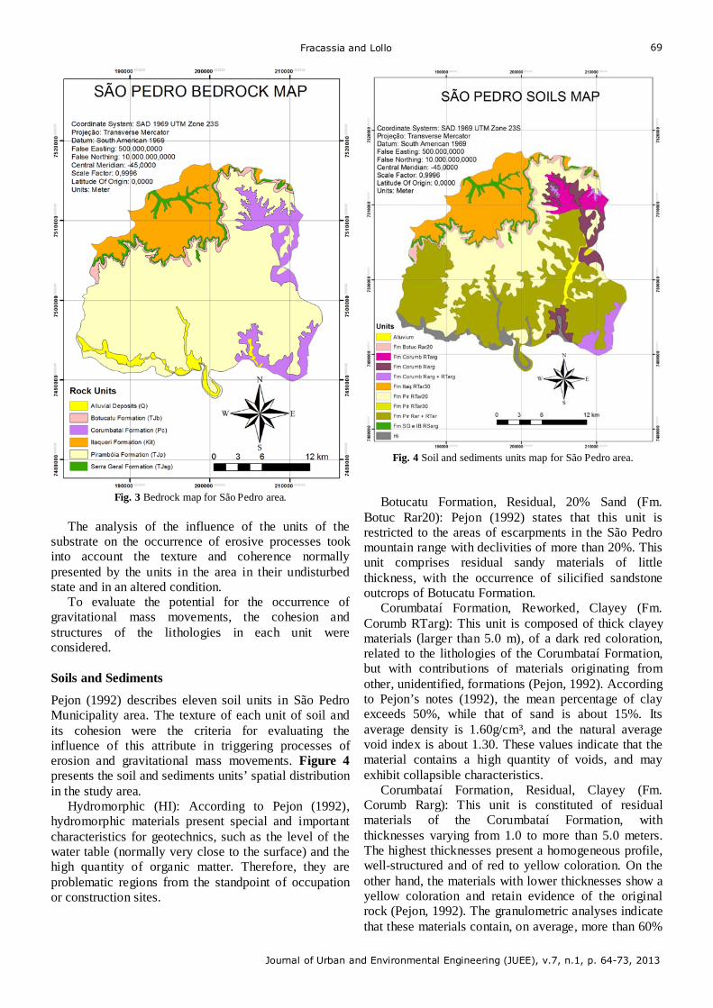
Fracassia and Lollo
Journal of Urban and Environmental Engineering (JUEE), v.7, n.1, p. 64-73, 2013
69
Fig. 3 Bedrock map for São Pedro area.
The analysis of the influence of the units of the
substrate on the occurrence of erosive processes took into account the texture and coherence normally presented by the units in the area in their undisturbed state and in an altered condition.
To evaluate the potential for the occurrence of gravitational mass movements, the cohesion and structures of the lithologies in each unit were considered. Soils and Sediments
Pejon (1992) describes eleven soil units in São Pedro Municipality area. The texture of each unit of soil and its cohesion were the criteria for evaluating the influence of this attribute in triggering processes of erosion and gravitational mass movements. Figure 4 presents the soil and sediments units’ spatial distribution in the study area.
Hydromorphic (HI): According to Pejon (1992), hydromorphic materials present special and important characteristics for geotechnics, such as the level of the water table (normally very close to the surface) and the high quantity of organic matter. Therefore, they are problematic regions from the standpoint of occupation or construction sites.
Fig. 4 Soil and sediments units map for São Pedro area.
Botucatu Formation, Residual, 20% Sand (Fm.
Botuc Rar20): Pejon (1992) states that this unit is restricted to the areas of escarpments in the São Pedro mountain range with declivities of more than 20%. This unit comprises residual sandy materials of little thickness, with the occurrence of silicified sandstone outcrops of Botucatu Formation.
Corumbataí Formation, Reworked, Clayey (Fm. Corumb RTarg): This unit is composed of thick clayey materials (larger than 5.0 m), of a dark red coloration, related to the lithologies of the Corumbataí Formation, but with contributions of materials originating from other, unidentified, formations (Pejon, 1992). According to Pejon’s notes (1992), the mean percentage of clay exceeds 50%, while that of sand is about 15%. Its average density is 1.60g/cm³, and the natural average void index is about 1.30. These values indicate that the material contains a high quantity of voids, and may exhibit collapsible characteristics.
Corumbataí Formation, Residual, Clayey (Fm. Corumb Rarg): This unit is constituted of residual materials of the Corumbataí Formation, with thicknesses varying from 1.0 to more than 5.0 meters. The highest thicknesses present a homogeneous profile, well-structured and of red to yellow coloration. On the other hand, the materials with lower thicknesses show a yellow coloration and retain evidence of the original rock (Pejon, 1992). The granulometric analyses indicate that these materials contain, on average, more than 60%
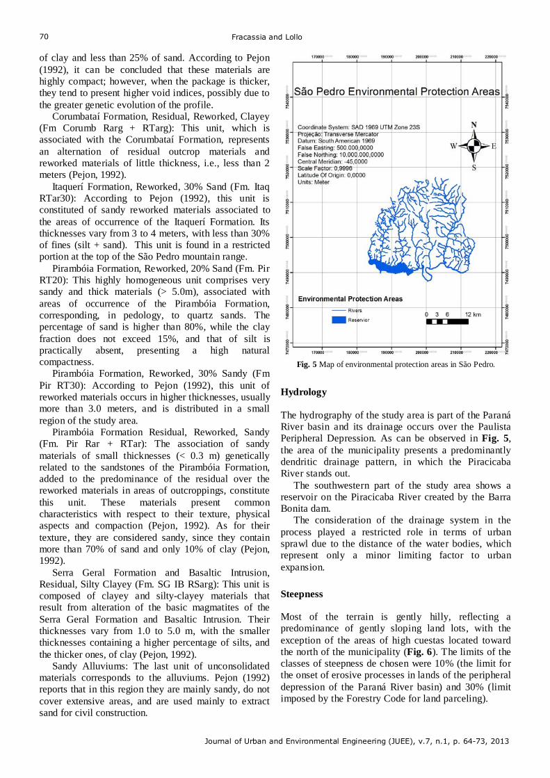
Fracassia and Lollo
Journal of Urban and Environmental Engineering (JUEE), v.7, n.1, p. 64-73, 2013
70
of clay and less than 25% of sand. According to Pejon (1992), it can be concluded that these materials are highly compact; however, when the package is thicker, they tend to present higher void indices, possibly due to the greater genetic evolution of the profile.
Corumbataí Formation, Residual, Reworked, Clayey (Fm Corumb Rarg + RTarg): This unit, which is associated with the Corumbataí Formation, represents an alternation of residual outcrop materials and reworked materials of little thickness, i.e., less than 2 meters (Pejon, 1992).
Itaquerí Formation, Reworked, 30% Sand (Fm. Itaq RTar30): According to Pejon (1992), this unit is constituted of sandy reworked materials associated to the areas of occurrence of the Itaquerí Formation. Its thicknesses vary from 3 to 4 meters, with less than 30% of fines (silt + sand). This unit is found in a restricted portion at the top of the São Pedro mountain range.
Pirambóia Formation, Reworked, 20% Sand (Fm. Pir RT20): This highly homogeneous unit comprises very sandy and thick materials (> 5.0m), associated with areas of occurrence of the Pirambóia Formation, corresponding, in pedology, to quartz sands. The percentage of sand is higher than 80%, while the clay fraction does not exceed 15%, and that of silt is practically absent, presenting a high natural compactness.
Pirambóia Formation, Reworked, 30% Sandy (Fm Pir RT30): According to Pejon (1992), this unit of reworked materials occurs in higher thicknesses, usually more than 3.0 meters, and is distributed in a small region of the study area.
Pirambóia Formation Residual, Reworked, Sandy (Fm. Pir Rar + RTar): The association of sandy materials of small thicknesses (< 0.3 m) genetically related to the sandstones of the Pirambóia Formation, added to the predominance of the residual over the reworked materials in areas of outcroppings, constitute this unit. These materials present common characteristics with respect to their texture, physical aspects and compaction (Pejon, 1992). As for their texture, they are considered sandy, since they contain more than 70% of sand and only 10% of clay (Pejon, 1992).
Serra Geral Formation and Basaltic Intrusion, Residual, Silty Clayey (Fm. SG IB RSarg): This unit is composed of clayey and silty-clayey materials that result from alteration of the basic magmatites of the Serra Geral Formation and Basaltic Intrusion. Their thicknesses vary from 1.0 to 5.0 m, with the smaller thicknesses containing a higher percentage of silts, and the thicker ones, of clay (Pejon, 1992).
Sandy Alluviums: The last unit of unconsolidated materials corresponds to the alluviums. Pejon (1992) reports that in this region they are mainly sandy, do not cover extensive areas, and are used mainly to extract sand for civil construction.
Fig. 5 Map of environmental protection areas in São Pedro.
Hydrology
The hydrography of the study area is part of the Paraná River basin and its drainage occurs over the Paulista Peripheral Depression. As can be observed in Fig. 5, the area of the municipality presents a predominantly dendritic drainage pattern, in which the Piracicaba River stands out.
The southwestern part of the study area shows a reservoir on the Piracicaba River created by the Barra Bonita dam.
The consideration of the drainage system in the process played a restricted role in terms of urban sprawl due to the distance of the water bodies, which represent only a minor limiting factor to urban expansion.
Steepness
Most of the terrain is gently hilly, reflecting a predominance of gently sloping land lots, with the exception of the areas of high cuestas located toward the north of the municipality (Fig. 6). The limits of the classes of steepness de chosen were 10% (the limit for the onset of erosive processes in lands of the peripheral depression of the Paraná River basin) and 30% (limit imposed by the Forestry Code for land parceling).
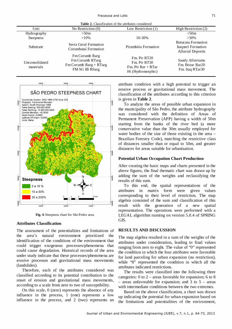
Fracassia and Lollo
Journal of Urban and Environmental Engineering (JUEE), v.7, n.1, p. 64-73, 2013
71
Table 2. Classification of the attributes considered
Unit No Restriction (0) Low Restriction (1) High Restriction (2) Hydrography >50m <50m
Steepness <10% 10-30% >30%
Substrate Serra Geral Formation Corumbataí Formation Pirambóia Formation
Botucatu Formation Itaquerí Formation Alluvial Deposits
Unconsolidated materials
Fm Corumb Rarg Fm Corumb RTarg
Fm Corumb Rarg + RTarg FM SG IB RSarg
Fm. Pir RT20 Fm. Pir RT30
Fm. Pir Rar + RTar Hi (Hydromorphic)
Sandy Alluviums Fm. Botuc Rar20 Fm. Itaq RTar30
Fig. 6 Steepness chart for São Pedro area.
Attributes Classification
The assessment of the potentialities and limitations of the area’s natural environment prioritized the identification of the conditions of the environment that could trigger exogenous processes/phenomena that could cause degradation. Historical records of the area under study indicate that these processes/phenomena are erosive processes and gravitational mass movements (landslides).
Therefore, each of the attributes considered was classified according to its potential contribution to the onset of erosion and gravitational mass movements, according to a scale from zero to two of susceptibility.
On this scale, 0 (zero) represents the absence of any influence in the process, 1 (one) represents a low influence in the process, and 2 (two) represents an
attribute condition with a high potential to trigger an erosive process or gravitational mass movement. The classification of the attributes according to this criterion is given in Table 2.
To analyze the areas of possible urban expansion in the municipality of São Pedro, the attribute hydrography was considered with the definition of Areas of Permanent Preservation (APP) having a width of 50m starting from the banks of the river bed (a more conservative value than the 30m usually employed for water bodies of the size of those existing in the area – Brazilian Forestry Code), matching the restrictive class of distances smaller than or equal to 50m, and greater distances for areas suitable for urbanization.
Potential Urban Occupation Chart Production
After creating the basic maps and charts presented in the above figures, the final thematic chart was drawn up by adding the sum of the weights and reclassifying the results of this sum.
To this end, the spatial representations of the attributes in matrix form were given values corresponding to their level of restriction. The map algebra consisted of the sum and classification of this result with the generation of a new spatial representation. The operations were performed with a LEGAL algorithm running on version 5.0.4 of SPRING GIS.
RESULTS AND DISCUSSION
The map algebra resulted in a sum of the weights of the attributes under consideration, leading to final values ranging from zero to eight. The value of “0” represented the condition in which the four attributes were favorable for land parceling for urban expansion (no restriction), while “8” represented the condition in which all the attributes indicated restrictions.
The results were classified into the following three categories: 0 to 2 – areas favorable for expansion; 6 to 8 – areas unfavorable for expansion; and 3 to 5 – areas with intermediate conditions between the two extremes.
Based on the above classification, a chart was drawn up indicating the potential for urban expansion based on the limitations and potentialities of the environment,
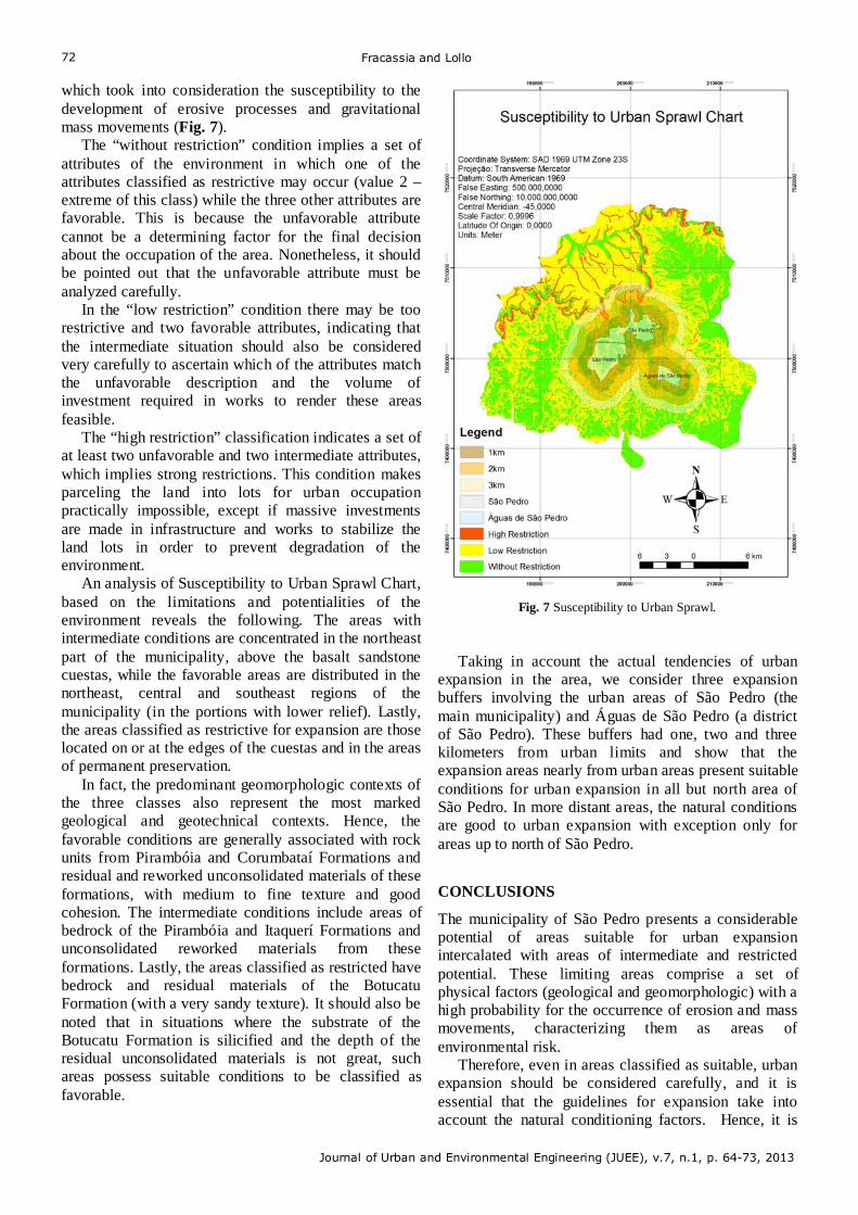
Fracassia and Lollo
Journal of Urban and Environmental Engineering (JUEE), v.7, n.1, p. 64-73, 2013
72
which took into consideration the susceptibility to the development of erosive processes and gravitational mass movements (Fig. 7).
The “without restriction” condition implies a set of attributes of the environment in which one of the attributes classified as restrictive may occur (value 2 – extreme of this class) while the three other attributes are favorable. This is because the unfavorable attribute cannot be a determining factor for the final decision about the occupation of the area. Nonetheless, it should be pointed out that the unfavorable attribute must be analyzed carefully.
In the “low restriction” condition there may be too restrictive and two favorable attributes, indicating that the intermediate situation should also be considered very carefully to ascertain which of the attributes match the unfavorable description and the volume of investment required in works to render these areas feasible.
The “high restriction” classification indicates a set of at least two unfavorable and two intermediate attributes, which implies strong restrictions. This condition makes parceling the land into lots for urban occupation practically impossible, except if massive investments are made in infrastructure and works to stabilize the land lots in order to prevent degradation of the environment.
An analysis of Susceptibility to Urban Sprawl Chart, based on the limitations and potentialities of the environment reveals the following. The areas with intermediate conditions are concentrated in the northeast part of the municipality, above the basalt sandstone cuestas, while the favorable areas are distributed in the northeast, central and southeast regions of the municipality (in the portions with lower relief). Lastly, the areas classified as restrictive for expansion are those located on or at the edges of the cuestas and in the areas of permanent preservation.
In fact, the predominant geomorphologic contexts of the three classes also represent the most marked geological and geotechnical contexts. Hence, the favorable conditions are generally associated with rock units from Pirambóia and Corumbataí Formations and residual and reworked unconsolidated materials of these formations, with medium to fine texture and good cohesion. The intermediate conditions include areas of bedrock of the Pirambóia and Itaquerí Formations and unconsolidated reworked materials from these formations. Lastly, the areas classified as restricted have bedrock and residual materials of the Botucatu Formation (with a very sandy texture). It should also be noted that in situations where the substrate of the Botucatu Formation is silicified and the depth of the residual unconsolidated materials is not great, such areas possess suitable conditions to be classified as favorable.
Fig. 7 Susceptibility to Urban Sprawl.
Taking in account the actual tendencies of urban expansion in the area, we consider three expansion buffers involving the urban areas of São Pedro (the main municipality) and Águas de São Pedro (a district of São Pedro). These buffers had one, two and three kilometers from urban limits and show that the expansion areas nearly from urban areas present suitable conditions for urban expansion in all but north area of São Pedro. In more distant areas, the natural conditions are good to urban expansion with exception only for areas up to north of São Pedro. CONCLUSIONS
The municipality of São Pedro presents a considerable potential of areas suitable for urban expansion intercalated with areas of intermediate and restricted potential. These limiting areas comprise a set of physical factors (geological and geomorphologic) with a high probability for the occurrence of erosion and mass movements, characterizing them as areas of environmental risk.
Therefore, even in areas classified as suitable, urban expansion should be considered carefully, and it is essential that the guidelines for expansion take into account the natural conditioning factors. Hence, it is
Fracassia and Lollo
Journal of Urban and Environmental Engineering (JUEE), v.7, n.1, p. 64-73, 2013
73
crucial for land use planning to be based on the quality and characteristics of the land in order to satisfy certain priorities and/or occupy any terrestrial space. It should be pointed out that this analysis was based on the conditions of the environment from the standpoint of erosion and gravitational mass movements, which are the most significant dynamic processes in the area in question. It should also be noted that in other realities (different municipalities or contexts of the environment), the selection of the attributes and the definition of the weights for each one may and/or should vary. Considering the buffers around urban areas we observe that only the areas in north of São present high restriction to urban expansion. Part of the results reported here coincide with the Master Plan of the municipality, which foresees as a zone of interest for urban expansion the area southeast of the urban seat of São Pedro. The analyses of this study, with their aforementioned restrictions, indicated the northeast, central and southeast portions of the municipality as areas with intermediate conditions for urban expansion, and the latter is the same one considered in the Master Plan. Lastly, it can be stated that this approach enabled aspects of the current legislation and the characteristics of the landscape to be analyzed jointly in evaluating the suitability of land use, thus serving as a strategy applicable to other situations.
REFERENCES
Braga, B. & Carvalho, P.F. (2004) City: space and citizen. In: Giometti, A.B.R. & Braga, R. Citizen Pedagogy: Formation Books: Geography Education. São Paulo: Universidade Estadual Paulista. (In Portuguese)
Brazil (2011) Provisional Measure #547/11. Union Official Diary, October 13th 2011. (In Portuguese)
Brazil (2012) #12,608/12 Law. Union Official Diary, April 11th 2012. (In Portuguese)
Burchell, R. & Mukhjerji, S. (2003) Conventional development versus managed growth: the costs of sprawl. American Journal of Public Health. 93 (9).
Carbonell, A. & Yaro, R. (2005) American spatial development and the new megalopolis - Land Lines. Lincoln Institute of Land Policy.
Carvalho, P.F. (2001) Environmental problems in social interest housing and cities. In: Carvalho, P.F. & Braga, R. Environmental management outlook in medium cities. Rio Claro: Universidade Estadual Paulista. (In Portuguese)
Fracassi, P.C. (2008) Urbanization and environmental and social impacts: São Pedro risk areas. Monograph. Rio Claro: Universidade Estadual Paulista. (In Portuguese)
IBGE (2000) 2000 Census. Brazilian Institute of Geography and Statistics. In: http://www.ibge.gov.br. Access: June 2010. (In Portuguese)
IPEA (2001) Brazilian Municipalities Database. Institute of Applied Economy Research. In: http://www.ipea.gov.br/portal/. Access: June 2010. (In Portuguese)
Johnson, M.P. (2001) Environmental impacts of urban sprawl: a survey of the literature and proposed research agenda. Environment and Planning A. 33: 717 - 735. 2001.
Limonad, E. (2007) Disperse Urbanization: another form of urban expression? Formation Journal, 1: (14). 2007.
Ojima, R. & Hogan, D.J. (2008) Urban growing and periurban occupation: spatial distribution of population in new environmental frontiers. In: 4th National Meeting of Post-graduation and Research in Environment and Society. Brasília. (In Portuguese)
Pejon, O.J. (1992) Engineering geological mapping of Piracicaba Sheet (1:100.000 Scale): methodological aspects of surveying attributes. PhD Thesis. São Paulo: Universidade Estadual de São Paulo. (In Portuguese)
Penteado, M.M. (1968) Geomorphology of center-east sector of Paulista Peripheral Depression. PhD Thesis. Rio Claro: Faculdade de Filosofia, Ciências e Letras. (In Portuguese)
Santos, M. (1996) Brazilian urbanization. (3rd ed.). São Paulo: Hucitec. (In Portuguese)
São Paulo. (1989) São Paulo State Constitution. In: http://www.al.sp.gov.br/repositorio/ legislacao/constituicao/1989/constituicao%20de%2005.10.1989.htm. Access. May 2010. (In Portuguese)
São Pedro (2008) São Pedro Master Plan – #15/08 Law. Public and Particular Works Department of São Pedro. (In Portuguese)
Camara, G., Souza, R.C.M., Freitas, U.M., Garrido, J. (1996) SPRING: Integrating remote sensing and GIS by object-oriented data modeling. Computers & Graphics, 20 (3): 395-403.
Valente, A.L.S. (1996). Using remote sensing in risk areas definition. 8th Brazilian Remote Sensing Symposium. Salvador. (In Portuguese)
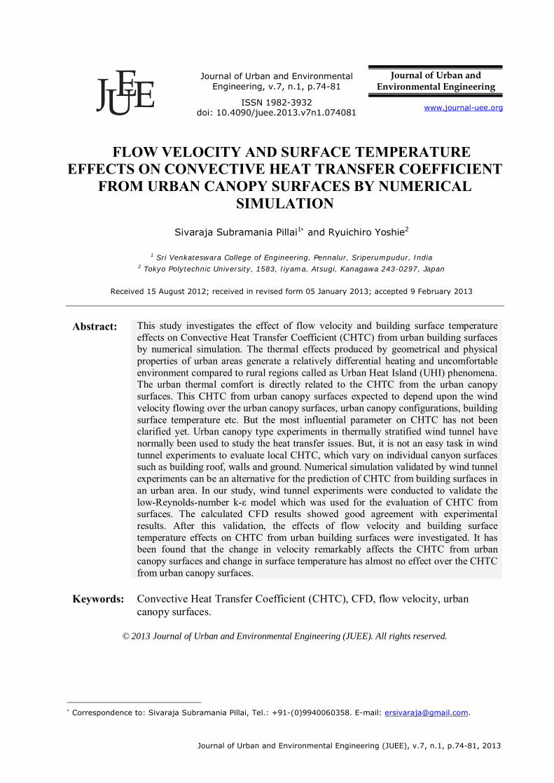
Journal of Urban and Environmental Engineering (JUEE), v.7, n.1, p.74-81, 2013
Journal of Urban and Environmental Engineering, v.7, n.1, p.74-81
Journal of Urban and Environmental Engineering
UEEJ ISSN 1982-3932
doi: 10.4090/juee.2013.v7n1.074081 www.journal-uee.org
FLOW VELOCITY AND SURFACE TEMPERATURE EFFECTS ON CONVECTIVE HEAT TRANSFER COEFFICIENT
FROM URBAN CANOPY SURFACES BY NUMERICAL SIMULATION
Sivaraja Subramania Pillai1 and Ryuichiro Yoshie2
1 Sri Venkateswara College of Engineering, Pennalur, Sriperumpudur, India
2 Tokyo Polytechnic University, 1583, Iiyama, Atsugi, Kanagawa 243-0297, Japan
Received 15 August 2012; received in revised form 05 January 2013; accepted 9 February 2013
Abstract: This study investigates the effect of flow velocity and building surface temperature
effects on Convective Heat Transfer Coefficient (CHTC) from urban building surfaces by numerical simulation. The thermal effects produced by geometrical and physical properties of urban areas generate a relatively differential heating and uncomfortable environment compared to rural regions called as Urban Heat Island (UHI) phenomena. The urban thermal comfort is directly related to the CHTC from the urban canopy surfaces. This CHTC from urban canopy surfaces expected to depend upon the wind velocity flowing over the urban canopy surfaces, urban canopy configurations, building surface temperature etc. But the most influential parameter on CHTC has not been clarified yet. Urban canopy type experiments in thermally stratified wind tunnel have normally been used to study the heat transfer issues. But, it is not an easy task in wind tunnel experiments to evaluate local CHTC, which vary on individual canyon surfaces such as building roof, walls and ground. Numerical simulation validated by wind tunnel experiments can be an alternative for the prediction of CHTC from building surfaces in an urban area. In our study, wind tunnel experiments were conducted to validate the low-Reynolds-number k-ε model which was used for the evaluation of CHTC from surfaces. The calculated CFD results showed good agreement with experimental results. After this validation, the effects of flow velocity and building surface temperature effects on CHTC from urban building surfaces were investigated. It has been found that the change in velocity remarkably affects the CHTC from urban canopy surfaces and change in surface temperature has almost no effect over the CHTC from urban canopy surfaces.
Keywords:
Convective Heat Transfer Coefficient (CHTC), CFD, flow velocity, urban canopy surfaces.
© 2013 Journal of Urban and Environmental Engineering (JUEE). All rights reserved.
Correspondence to: Sivaraja Subramania Pillai, Tel.: +91-(0)9940060358. E-mail: [email protected].
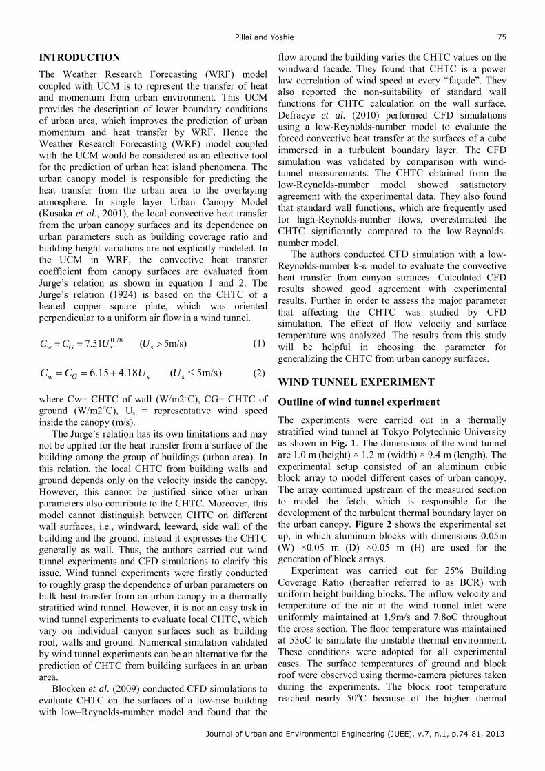
Pillai and Yoshie
Journal of Urban and Environmental Engineering (JUEE), v.7, n.1, p.74-81, 2013
75
INTRODUCTION
The Weather Research Forecasting (WRF) model coupled with UCM is to represent the transfer of heat and momentum from urban environment. This UCM provides the description of lower boundary conditions of urban area, which improves the prediction of urban momentum and heat transfer by WRF. Hence the Weather Research Forecasting (WRF) model coupled with the UCM would be considered as an effective tool for the prediction of urban heat island phenomena. The urban canopy model is responsible for predicting the heat transfer from the urban area to the overlaying atmosphere. In single layer Urban Canopy Model (Kusaka et al., 2001), the local convective heat transfer from the urban canopy surfaces and its dependence on urban parameters such as building coverage ratio and building height variations are not explicitly modeled. In the UCM in WRF, the convective heat transfer coefficient from canopy surfaces are evaluated from Jurge’s relation as shown in equation 1 and 2. The Jurge’s relation (1924) is based on the CHTC of a heated copper square plate, which was oriented perpendicular to a uniform air flow in a wind tunnel.
0.787.51 ( 5m/s)w G s sC C U U (1)
6.15 4.18 ( 5m/s)w G s sC C U U (2)
where Cw= CHTC of wall (W/m2oC), CG= CHTC of ground (W/m2oC), Us = representative wind speed inside the canopy (m/s).
The Jurge’s relation has its own limitations and may not be applied for the heat transfer from a surface of the building among the group of buildings (urban area). In this relation, the local CHTC from building walls and ground depends only on the velocity inside the canopy. However, this cannot be justified since other urban parameters also contribute to the CHTC. Moreover, this model cannot distinguish between CHTC on different wall surfaces, i.e., windward, leeward, side wall of the building and the ground, instead it expresses the CHTC generally as wall. Thus, the authors carried out wind tunnel experiments and CFD simulations to clarify this issue. Wind tunnel experiments were firstly conducted to roughly grasp the dependence of urban parameters on bulk heat transfer from an urban canopy in a thermally stratified wind tunnel. However, it is not an easy task in wind tunnel experiments to evaluate local CHTC, which vary on individual canyon surfaces such as building roof, walls and ground. Numerical simulation validated by wind tunnel experiments can be an alternative for the prediction of CHTC from building surfaces in an urban area.
Blocken et al. (2009) conducted CFD simulations to evaluate CHTC on the surfaces of a low-rise building with low–Reynolds-number model and found that the
flow around the building varies the CHTC values on the windward facade. They found that CHTC is a power law correlation of wind speed at every “façade”. They also reported the non-suitability of standard wall functions for CHTC calculation on the wall surface. Defraeye et al. (2010) performed CFD simulations using a low-Reynolds-number model to evaluate the forced convective heat transfer at the surfaces of a cube immersed in a turbulent boundary layer. The CFD simulation was validated by comparison with wind-tunnel measurements. The CHTC obtained from the low-Reynolds-number model showed satisfactory agreement with the experimental data. They also found that standard wall functions, which are frequently used for high-Reynolds-number flows, overestimated the CHTC significantly compared to the low-Reynolds-number model.
The authors conducted CFD simulation with a low-Reynolds-number k-ε model to evaluate the convective heat transfer from canyon surfaces. Calculated CFD results showed good agreement with experimental results. Further in order to assess the major parameter that affecting the CHTC was studied by CFD simulation. The effect of flow velocity and surface temperature was analyzed. The results from this study will be helpful in choosing the parameter for generalizing the CHTC from urban canopy surfaces.
WIND TUNNEL EXPERIMENT
Outline of wind tunnel experiment
The experiments were carried out in a thermally stratified wind tunnel at Tokyo Polytechnic University as shown in Fig. 1. The dimensions of the wind tunnel are 1.0 m (height) × 1.2 m (width) × 9.4 m (length). The experimental setup consisted of an aluminum cubic block array to model different cases of urban canopy. The array continued upstream of the measured section to model the fetch, which is responsible for the development of the turbulent thermal boundary layer on the urban canopy. Figure 2 shows the experimental set up, in which aluminum blocks with dimensions 0.05m (W) ×0.05 m (D) ×0.05 m (H) are used for the generation of block arrays.
Experiment was carried out for 25% Building Coverage Ratio (hereafter referred to as BCR) with uniform height building blocks. The inflow velocity and temperature of the air at the wind tunnel inlet were uniformly maintained at 1.9m/s and 7.8oC throughout the cross section. The floor temperature was maintained at 53oC to simulate the unstable thermal environment. These conditions were adopted for all experimental cases. The surface temperatures of ground and block roof were observed using thermo-camera pictures taken during the experiments. The block roof temperature reached nearly 50oC because of the higher thermal
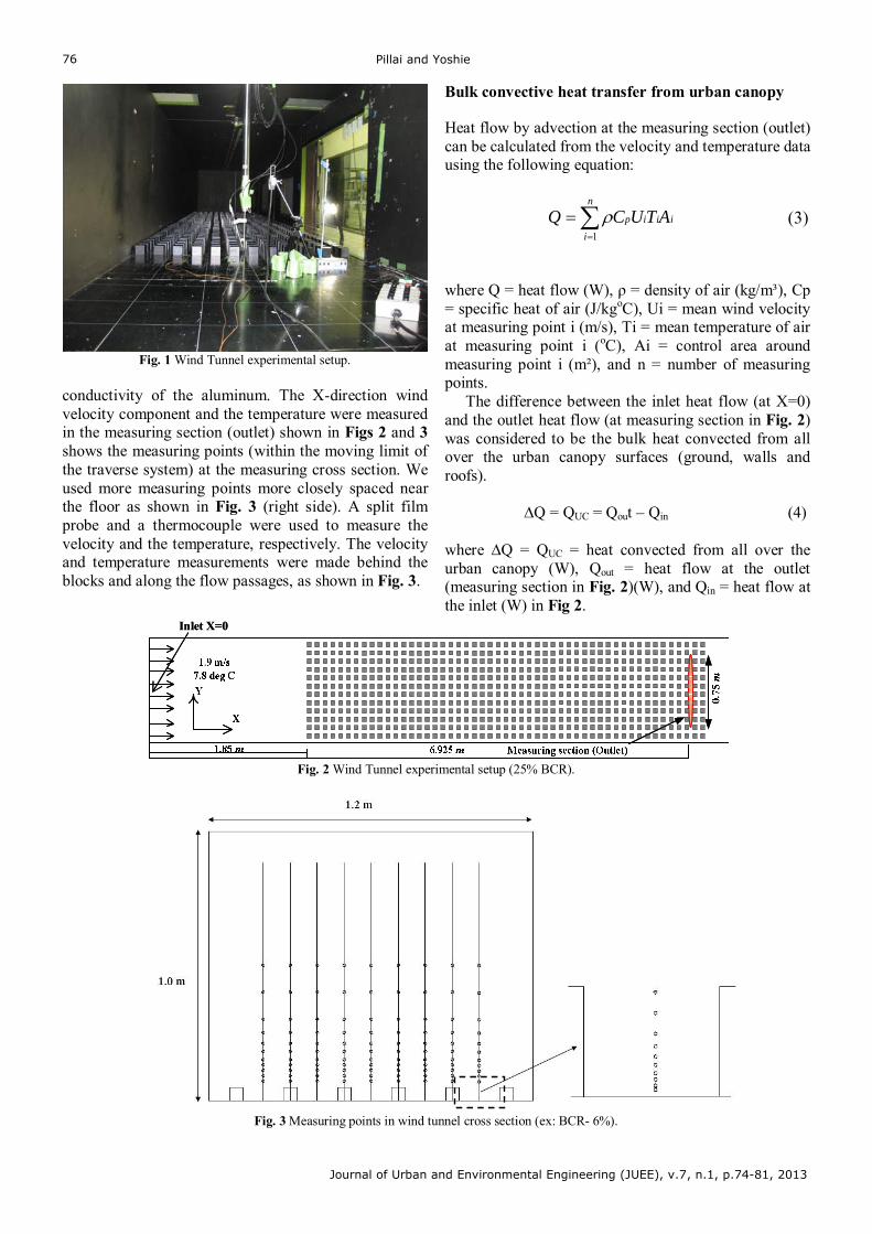
Pillai and Yoshie
Journal of Urban and Environmental Engineering (JUEE), v.7, n.1, p.74-81, 2013
76
Fig. 1 Wind Tunnel experimental setup.
conductivity of the aluminum. The X-direction wind velocity component and the temperature were measured in the measuring section (outlet) shown in Figs 2 and 3 shows the measuring points (within the moving limit of the traverse system) at the measuring cross section. We used more measuring points more closely spaced near the floor as shown in Fig. 3 (right side). A split film probe and a thermocouple were used to measure the velocity and the temperature, respectively. The velocity and temperature measurements were made behind the blocks and along the flow passages, as shown in Fig. 3.
Bulk convective heat transfer from urban canopy
Heat flow by advection at the measuring section (outlet) can be calculated from the velocity and temperature data using the following equation:
n
i
iiip ATUCQ1
(3)
where Q = heat flow (W), ρ = density of air (kg/m³), Cp = specific heat of air (J/kgoC), Ui = mean wind velocity at measuring point i (m/s), Ti = mean temperature of air at measuring point i (oC), Ai = control area around measuring point i (m²), and n = number of measuring points.
The difference between the inlet heat flow (at X=0) and the outlet heat flow (at measuring section in Fig. 2) was considered to be the bulk heat convected from all over the urban canopy surfaces (ground, walls and roofs).
∆Q = QUC = Qout – Qin (4)
where ∆Q = QUC = heat convected from all over the urban canopy (W), Qout = heat flow at the outlet (measuring section in Fig. 2)(W), and Qin = heat flow at the inlet (W) in Fig 2.
Inlet X=0 Inlet X=0
Fig. 2 Wind Tunnel experimental setup (25% BCR).
Fig. 3 Measuring points in wind tunnel cross section (ex: BCR- 6%).
Pillai and Yoshie
Journal of Urban and Environmental Engineering (JUEE), v.7, n.1, p.74-81, 2013
77
x
Y0.
025m
0.05
m
0.05m 0.1m
x
Y0.
025m
0.05
m
0.05m 0.1m
Fig. 4a Grid arrangement in horizontal plane (ex : uniform height, BCR-11% case).
x
Z
0.05
m
0.05m 0.1m
x
Z
0.05
m
0.05m 0.1m
Fig. 4b Grid arrangement in vertical section (ex : uniform height, BCR-11% case).
CFD Simulation General outline of numerical simulation and boundary conditions
For the calculation of complex turbulent flows with separation and heat transfer, Abe et al. (1994, 1995) developed a new low-Reynolds number turbulence model for flow field and thermal field. This model quite successfully predicts the separating and reattaching flows in the downstream of a backward-facing step, which involve most of the important physical phenomenon of complex turbulent flow around obstacles. Thus, the authors considered this Low Reynolds number k-ε model was suitable for urban canopy simulations.
Figures 4a and 4b shows the grid arrangement in the horizontal plane and vertical section (For example: BCR-11% case with uniform height buildings), respectively. The computational domain was an exact replica of the wind tunnel in windward length and vertical height. Minimum width was selected by considering symmetry in the Y direction. As shown in Figs 4a and 4b the domain has structured grids with very fine mesh near the wall surfaces. Distance between wall surface and first mesh line was 0.2 mm. As a result, non-dimensional distances from the wall surfaces Y+ were below 1.0 for most of the first fluid cells close to
the wall surfaces. y+ is defined as follows:
yu
y * (5)
where = frictional velocity at the surface (m/s), y=distance between the wall surface and the first fluid cell (m), and ν=kienematic viscosity of air (m2/s). The maximal value of y+ was in the range of ‘2’ at edge of the windward wall, sidewall and roof of the first block in the upstream region where the frictional velocity at the surface is higher (higher wall shear stress). We conducted grid sensitivity analyses using fine mesh (1939(x)×30(y)×67(z) = 3 897 390) and coarse mesh (1378(x)×20(y)×59(z) = 1 626 040) for BCR25% uniform case. The differences between wind velocities and temperature profiles and convective heat transfer for the calculated results of the fine mesh and the coarse mesh were extremely small. Thus we judged that the grid resolution of the fine mesh was sufficient, and after that grids with similar resolution to the above fine mesh were used for other calculation cases.
Calculation conditions (For example: BCR-11% case with uniform height buildings) are shown in Table 1. No slip boundary conditions were applied for wall shear stress. For thermal boundary conditions, surface temperatures were prescribed and heat conduction boundary condition was applied for heat flux on the wall surfaces. The surface temperature for various
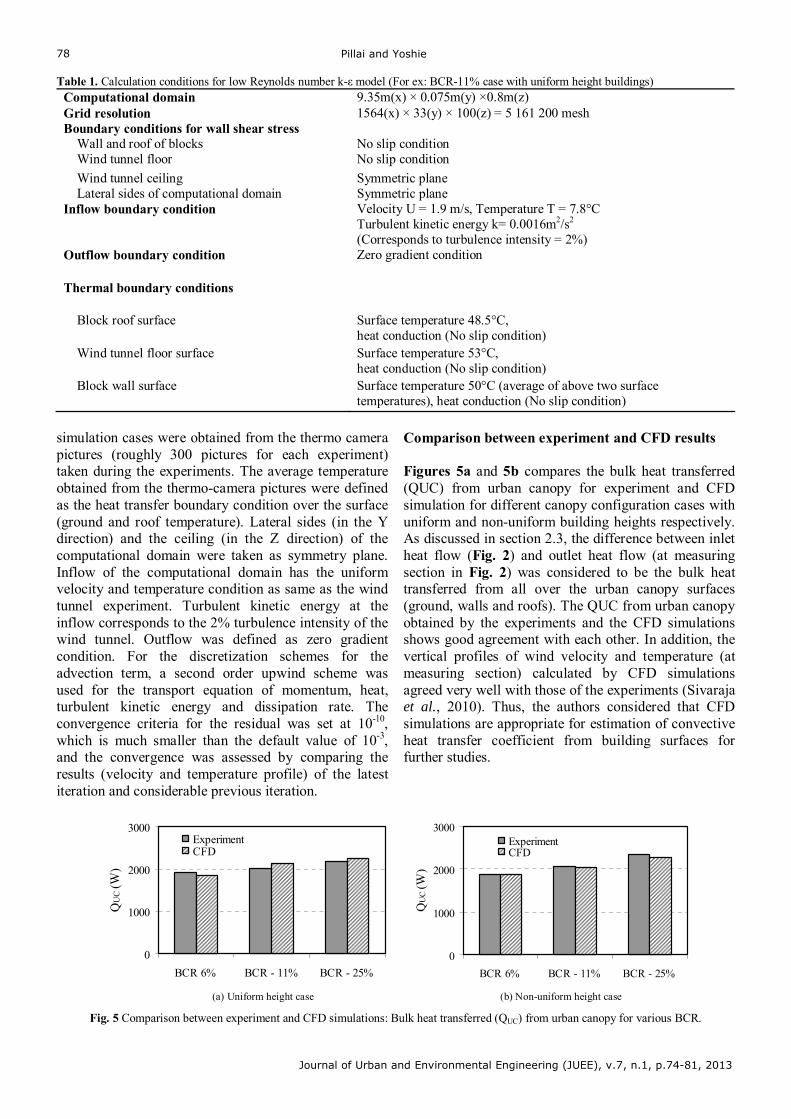
Pillai and Yoshie
Journal of Urban and Environmental Engineering (JUEE), v.7, n.1, p.74-81, 2013
78
Table 1. Calculation conditions for low Reynolds number k-ε model (For ex: BCR-11% case with uniform height buildings) Computational domain 9.35m(x) × 0.075m(y) ×0.8m(z) Grid resolution 1564(x) × 33(y) × 100(z) = 5 161 200 mesh Boundary conditions for wall shear stress
Wall and roof of blocks No slip condition Wind tunnel floor No slip condition
Wind tunnel ceiling Symmetric plane Lateral sides of computational domain Symmetric plane
Inflow boundary condition Velocity U = 1.9 m/s, Temperature T = 7.8°C Turbulent kinetic energy k= 0.0016m2/s2 (Corresponds to turbulence intensity = 2%)
Outflow boundary condition Zero gradient condition
Thermal boundary conditions
Block roof surface Surface temperature 48.5°C, heat conduction (No slip condition)
Wind tunnel floor surface Surface temperature 53°C, heat conduction (No slip condition)
Block wall surface Surface temperature 50°C (average of above two surface temperatures), heat conduction (No slip condition)
simulation cases were obtained from the thermo camera pictures (roughly 300 pictures for each experiment) taken during the experiments. The average temperature obtained from the thermo-camera pictures were defined as the heat transfer boundary condition over the surface (ground and roof temperature). Lateral sides (in the Y direction) and the ceiling (in the Z direction) of the computational domain were taken as symmetry plane. Inflow of the computational domain has the uniform velocity and temperature condition as same as the wind tunnel experiment. Turbulent kinetic energy at the inflow corresponds to the 2% turbulence intensity of the wind tunnel. Outflow was defined as zero gradient condition. For the discretization schemes for the advection term, a second order upwind scheme was used for the transport equation of momentum, heat, turbulent kinetic energy and dissipation rate. The convergence criteria for the residual was set at 10-10, which is much smaller than the default value of 10-3, and the convergence was assessed by comparing the results (velocity and temperature profile) of the latest iteration and considerable previous iteration.
Comparison between experiment and CFD results
Figures 5a and 5b compares the bulk heat transferred (QUC) from urban canopy for experiment and CFD simulation for different canopy configuration cases with uniform and non-uniform building heights respectively. As discussed in section 2.3, the difference between inlet heat flow (Fig. 2) and outlet heat flow (at measuring section in Fig. 2) was considered to be the bulk heat transferred from all over the urban canopy surfaces (ground, walls and roofs). The QUC from urban canopy obtained by the experiments and the CFD simulations shows good agreement with each other. In addition, the vertical profiles of wind velocity and temperature (at measuring section) calculated by CFD simulations agreed very well with those of the experiments (Sivaraja et al., 2010). Thus, the authors considered that CFD simulations are appropriate for estimation of convective heat transfer coefficient from building surfaces for further studies.
0
1000
2000
3000
BCR 6% BCR - 11% BCR - 25%
QU
C (
W)
ExperimentCFD
0
1000
2000
3000
BCR 6% BCR - 11% BCR - 25%
QU
C (
W)
ExperimentCFD
(a) Uniform height case (b) Non-uniform height case
Fig. 5 Comparison between experiment and CFD simulations: Bulk heat transferred (QUC) from urban canopy for various BCR.
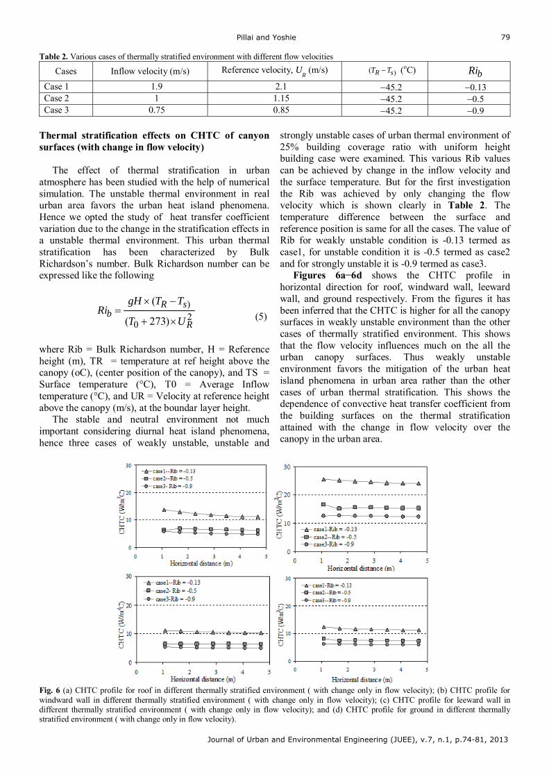
Pillai and Yoshie
Journal of Urban and Environmental Engineering (JUEE), v.7, n.1, p.74-81, 2013
79
Table 2. Various cases of thermally stratified environment with different flow velocities
Cases Inflow velocity (m/s) Reference velocity, UR (m/s) )( R sT T (oC) bRi
Case 1 1.9 2.1 45.2 0.13 Case 2 1 1.15 45.2 0.5 Case 3 0.75 0.85 45.2 0.9
Thermal stratification effects on CHTC of canyon surfaces (with change in flow velocity)
The effect of thermal stratification in urban
atmosphere has been studied with the help of numerical simulation. The unstable thermal environment in real urban area favors the urban heat island phenomena. Hence we opted the study of heat transfer coefficient variation due to the change in the stratification effects in a unstable thermal environment. This urban thermal stratification has been characterized by Bulk Richardson’s number. Bulk Richardson number can be expressed like the following
)2
0
(
( 273)
R sb
R
gH T TRi
T U
(5)
where Rib = Bulk Richardson number, H = Reference height (m), TR = temperature at ref height above the canopy (oC), (center position of the canopy), and TS = Surface temperature (°C), T0 = Average Inflow temperature (°C), and UR = Velocity at reference height above the canopy (m/s), at the boundar layer height.
The stable and neutral environment not much important considering diurnal heat island phenomena, hence three cases of weakly unstable, unstable and
strongly unstable cases of urban thermal environment of 25% building coverage ratio with uniform height building case were examined. This various Rib values can be achieved by change in the inflow velocity and the surface temperature. But for the first investigation the Rib was achieved by only changing the flow velocity which is shown clearly in Table 2. The temperature difference between the surface and reference position is same for all the cases. The value of Rib for weakly unstable condition is -0.13 termed as case1, for unstable condition it is -0.5 termed as case2 and for strongly unstable it is -0.9 termed as case3.
Figures 6a−6d shows the CHTC profile in horizontal direction for roof, windward wall, leeward wall, and ground respectively. From the figures it has been inferred that the CHTC is higher for all the canopy surfaces in weakly unstable environment than the other cases of thermally stratified environment. This shows that the flow velocity influences much on the all the urban canopy surfaces. Thus weakly unstable environment favors the mitigation of the urban heat island phenomena in urban area rather than the other cases of urban thermal stratification. This shows the dependence of convective heat transfer coefficient from the building surfaces on the thermal stratification attained with the change in flow velocity over the canopy in the urban area.
Fig. 6 (a) CHTC profile for roof in different thermally stratified environment ( with change only in flow velocity); (b) CHTC profile for windward wall in different thermally stratified environment ( with change only in flow velocity); (c) CHTC profile for leeward wall in different thermally stratified environment ( with change only in flow velocity); and (d) CHTC profile for ground in different thermally stratified environment ( with change only in flow velocity).
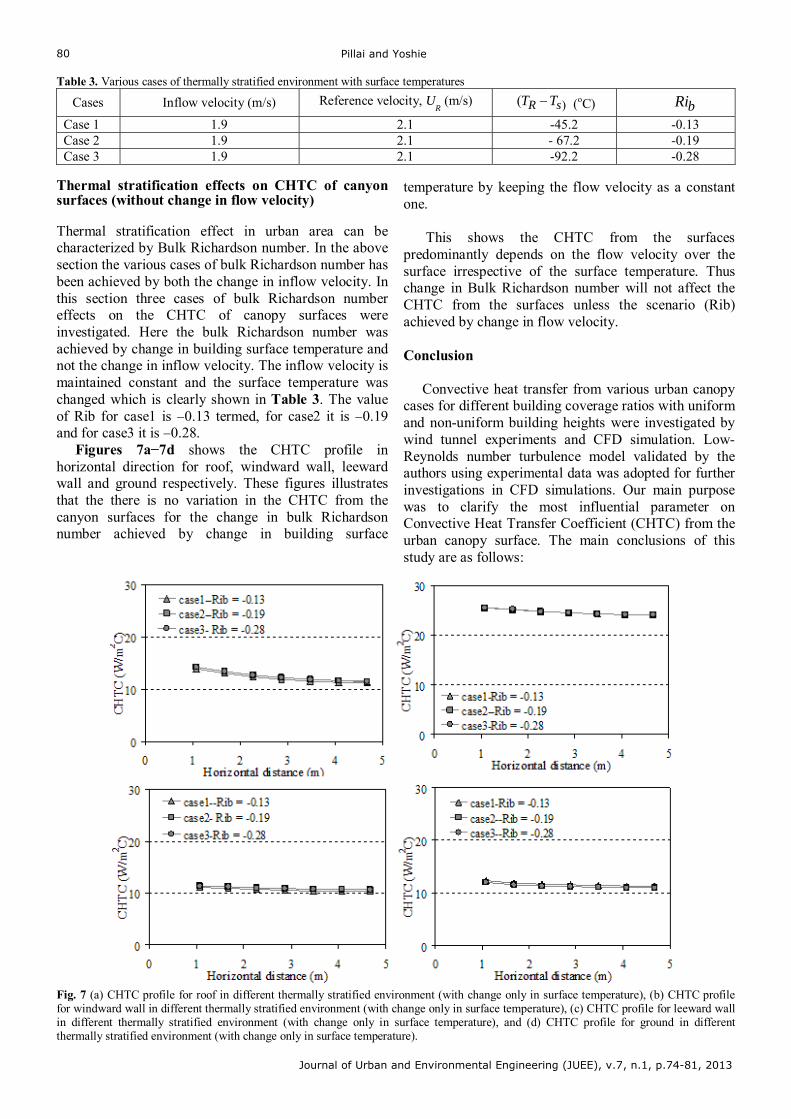
Pillai and Yoshie
Journal of Urban and Environmental Engineering (JUEE), v.7, n.1, p.74-81, 2013
80
Table 3. Various cases of thermally stratified environment with surface temperatures
Cases Inflow velocity (m/s) Reference velocity, UR (m/s) )( R sT T (oC) bRi
Case 1 1.9 2.1 -45.2 -0.13 Case 2 1.9 2.1 - 67.2 -0.19 Case 3 1.9 2.1 -92.2 -0.28
Thermal stratification effects on CHTC of canyon surfaces (without change in flow velocity) Thermal stratification effect in urban area can be characterized by Bulk Richardson number. In the above section the various cases of bulk Richardson number has been achieved by both the change in inflow velocity. In this section three cases of bulk Richardson number effects on the CHTC of canopy surfaces were investigated. Here the bulk Richardson number was achieved by change in building surface temperature and not the change in inflow velocity. The inflow velocity is maintained constant and the surface temperature was changed which is clearly shown in Table 3. The value of Rib for case1 is 0.13 termed, for case2 it is 0.19 and for case3 it is 0.28.
Figures 7a−7d shows the CHTC profile in horizontal direction for roof, windward wall, leeward wall and ground respectively. These figures illustrates that the there is no variation in the CHTC from the canyon surfaces for the change in bulk Richardson number achieved by change in building surface
temperature by keeping the flow velocity as a constant one.
This shows the CHTC from the surfaces
predominantly depends on the flow velocity over the surface irrespective of the surface temperature. Thus change in Bulk Richardson number will not affect the CHTC from the surfaces unless the scenario (Rib) achieved by change in flow velocity. Conclusion
Convective heat transfer from various urban canopy
cases for different building coverage ratios with uniform and non-uniform building heights were investigated by wind tunnel experiments and CFD simulation. Low-Reynolds number turbulence model validated by the authors using experimental data was adopted for further investigations in CFD simulations. Our main purpose was to clarify the most influential parameter on Convective Heat Transfer Coefficient (CHTC) from the urban canopy surface. The main conclusions of this study are as follows:
Fig. 7 (a) CHTC profile for roof in different thermally stratified environment (with change only in surface temperature), (b) CHTC profile for windward wall in different thermally stratified environment (with change only in surface temperature), (c) CHTC profile for leeward wall in different thermally stratified environment (with change only in surface temperature), and (d) CHTC profile for ground in different thermally stratified environment (with change only in surface temperature).
Pillai and Yoshie
Journal of Urban and Environmental Engineering (JUEE), v.7, n.1, p.74-81, 2013
81
1. Prediction of bulk heat transfer by CFD simulation with Low-Reynolds number k-εmodel is satisfactory when compared with the experimental results.
2. It has been found that the change in velocity
over the canopy remarkably affects the CHTC from urban canopy surfaces and change in surface temperature has almost no effect over the CHTC from urban canopy surfaces.
3. For the generalization of CHTC for urban
canopy surfaces, velocity has to be considered in priority and which was found to be the most influential parameter affecting CHTC from the surfaces.
4. Convective heat transfer coefficient (CHTC)
from individual canyon surfaces will be generalized for various urban canopy cases with the help of the parametric studies performed by CFD simulation (future work). The different cases for parametric studies will be selected by varying the Building Coverage Ratio (BCR), the height of the buildings, Reynolds number and Bulk Richardson number (by varying inflow velocity). Various simulation case results will be employed to generalize the CHTC from the canyon surfaces. The CHTC expressed as local Nusselt number will be generalized with variables like local canopy velocity expressed in local Reynolds number, building coverage ratio, height ratio) and canopy Richardson number. Inclusion of this generalized expression for individual urban canopy surfaces in UCM will be expected to increase the prediction accuracy of urban heat transfer by WRF.
Acknowledgements This study was funded by the Ministry of Education, Culture, Sports, Science and Technology, Japan, through the Global Center of Excellence Program, 2008-2013 which is gratefully acknowledged. Also we would like to express our
gratitude to Japan Society for the Promotion of Science (JSPS) for Grant-in-Aid for Scientific Research (B), No. 21360283.
REFERENCES
Abe, K., Kondoh, T., Nagano, Y. (1994) A new turbulence model
for predicting fluid flow and heat transfer in separating and reattaching flows-I.Flow field calculations. International Journal of Heat and Mass transfer. 37(1), 139-151.
Abe, K., Kondoh, T., Nagano, Y. (1995) A new turbulence model for predicting fluid flow and heat transfer in separating and reattaching flows-II. Thermal field calculations. International Journal of Heat and Mass transfer. 38(8), 1467-1481.
Blocken, B., Defraeye, T., Derome, D., Carmeliet, J. (2009) High-resolution CFD simulations of forced convective heat transfer coefficients at the facade of a low-rise building. Building and Environment 44(12), 2396-2412.
Defraeye, T., Blocken, B., Carmeliet, J. (2010) CFD analysis of convective heat transfer at the surfaces of a cube immersed in a turbulent boundary layer. International Journal of Heat and Mass Transfer. 53(2) 297–308.
Jürges, W. (1924) Der Wärmeübergang an einer ebenen Wand (heat transfer at a plane wall). Beihefte zum, Gesundheits-Ingenieur 1 (19).
Kusaka, H., Kondo, H., Kikegawa, Y.. Kimura, F. (2001) A Simple Single –layer urban canopy model for Atmospheric models : comparison with multi-layer and slab models”, Boundary Layer Meteorology -101,329-358.
Launder. B.E. Numerical computation of convective heat transfer in complex turbulent flows: time to abandon wall functions ?”, International Journal of Heat and Mass transfer, Vol. 27, No. 9 (1984), pp. 1485-1491.
Marciotto, E., Amauri, P., Oliveira, S., Hanna, R. (2010) Modeling study of the aspect ratio influence on urban canopy energy fluxes with a modified wall canyon energy budget scheme. Building and Environment 45, 2497-2505.
Pillai, S.S., Yoshie, R. (2012) Experimental and numerical studies on convective heat transfer from various urban canopy configurations”- Journal of Wind Engineering and Industrial Aerodynamics 104–106(4), 447-454.
Pillai, S.S., Yoshie, R., Chung, J. (2010) Experimental and computational studies of heat transfer from urban canopy and its dependence on urban parameters. Proc. Fifth International Symposium on Computational Wind Engineering (CWE 2010), TS6-1, May 2010, North Carolina, United States of America.
Pillai, S.S., Yoshie, R. (2011) Experimental and numerical studies on convective heat transfer from various urban canopy configurations. Abs No. 399, Proc. Thirteenth International conference on wind engineering (ICWE13), July 2011, The Netherlands.
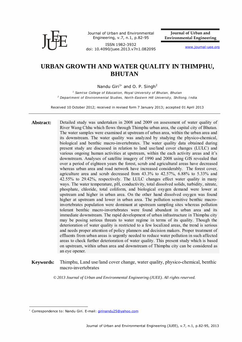
Giri and Singh
Journal of Urban and Environmental Engineering (JUEE), v.7, n.1, p.82-95, 2013
82
Journal of Urban and Environmental Engineering, v.7, n.1, p.82-95
Journal of Urban and Environmental Engineering
UEEJ ISSN 1982-3932
doi: 10.4090/juee.2013.v7n1.082095 www.journal-uee.org
URBAN GROWTH AND WATER QUALITY IN THIMPHU, BHUTAN
Nandu Giri1 and O. P. Singh2
1 Samtse College of Education, Royal University of Bhutan, Bhutan 2 Department of Environmental Studies, North-Eastern Hill University, Shillong, India
Received 10 October 2012; received in revised form 7 January 2013; accepted 01 April 2013
Abstract: Detailed study was undertaken in 2008 and 2009 on assessment of water quality of
River Wang Chhu which flows through Thimphu urban area, the capital city of Bhutan. The water samples were examined at upstream of urban area, within the urban area and its downstream. The water quality was analyzed by studying the physico-chemical, biological and benthic macro-invertebrates. The water quality data obtained during present study are discussed in relation to land use/land cover changes (LULC) and various ongoing human activities at upstream, within the each activity areas and it’s downstream. Analyses of satellite imagery of 1990 and 2008 using GIS revealed that over a period of eighteen years the forest, scrub and agricultural areas have decreased whereas urban area and road network have increased considerably. The forest cover, agriculture area and scrub decreased from 43.3% to 42.57%, 6.88% to 5.33% and 42.55% to 29.42%, respectively. The LULC changes effect water quality in many ways. The water temperature, pH, conductivity, total dissolved solids, turbidity, nitrate, phosphate, chloride, total coliform, and biological oxygen demand were lower at upstream and higher in urban area. On the other hand dissolved oxygen was found higher at upstream and lower in urban area. The pollution sensitive benthic macro-invertebrates population were dominant at upstream sampling sites whereas pollution tolerant benthic macro-invertebrates were found abundant in urban area and its immediate downstream. The rapid development of urban infrastructure in Thimphu city may be posing serious threats to water regime in terms of its quality. Though the deterioration of water quality is restricted to a few localized areas, the trend is serious and needs proper attention of policy planners and decision makers. Proper treatment of effluents from urban areas is urgently needed to reduce water pollution in such affected areas to check further deterioration of water quality. This present study which is based on upstream, within urban area and downstream of Thimphu city can be considered as an eye opener.
Keywords:
Thimphu, Land use/land cover change, water quality, physico-chemical, benthic macro-invertebrates
© 2013 Journal of Urban and Environmental Engineering (JUEE). All rights reserved.
Correspondence to: Nandu Giri. E-mail: [email protected]
Giri and Singh
Journal of Urban and Environmental Engineering (JUEE), v.7, n.1, p.82-95, 2013
83
INTRODUCTION
Water occupies a special place among other natural resources found on earth. It is indeed a valuable natural resource vital to the existence of all living organisms. It is an indispensable liquid required for several purposes such as drinking, sanitation, irrigation, navigation, aquaculture, recreation, industrial uses etc. The water bodies are closely related to human life and his livelihood. The metabolic activities essential for life take place in aqueous medium inside the living body.
All enzymes, hormones and other biomolecules exist and function in presence of water. Water dissolves nutrients and distributes them to cells, regulates body temperature, supports structures, and removes waste products. Thus, all forms of life on earth depend on water and all living things, from plants to animals, from desert dwellers to aquatic inhabitants and from microscopic bacteria to gigantic whale, need water to survive. It is believed that life first originated in water. Water forms three-fourth of the weight of a living cell (United Nations Environment Programme (UNEP) Report, 2006). The health and well-being of all the living beings on earth is closely tied up with the quality of water (United Nations World Water Assessment Programme (UN-WWAP) Report, 2003).
Currently, humanity is facing a serious water crisis (UN-WWAP, 2003). The United Nations World Water Assessment Programme Report (2003) states that water crises of availability, degradation, conservation and sustainability can be observed more pronouncedly in developing countries all over the world. All indicators suggest that the situation is worsening day by day and it is going to be alarming unless corrective measures are taken soon. The world is facing a number of challenges with regard to the availability, accessibility, use and sustainability of freshwater resources. This would result in serious implications for present and future generations of humanity and also for natural ecosystems. It is estimated that at present 2.8 billion people live under conditions of water stress and by 2030 almost half the world population will live under these conditions if effective measures are not implemented (UNEP, 2009; Bates et al., 2008; OECD, 2008).
Freshwater bodies vary from streams and rivulets to huge rivers, ponds and lakes to reservoirs and recreational pools. These aquatic ecosystems are characterized by complex interactions between abiotic and biotic components of the water system. Thus, study on physico-chemical characteristics and biotic attributes of different water bodies is essential to understand the quality of water. Such studies in relation to anthropogenic land use changes and diversified human activities taking place in the catchment area are keys to understanding the causes and extent of degradation of
water resources. Keeping this view in mind, a study on water quality in relation to land use/land cover changes was carried out during 2008 and 2009 in Bhutan, one of Asia’s smallest nations situated on the southern slope of the eastern Himalayas (latitude 26˚40’ − 28˚20’N; longitude 88˚45’ − 92˚25’E). It has a geographical area of 38 394 km² with mountainous and heavily forested landscapes. The present study was carried out at upstream of urban area, within the urban area and its downstream of Thimphu, the capital city of Bhutan.
STUDY AREA, MATERIAL AND METHODS Thimphu, the capital of Bhutan is located in the North West at an altitude of 2320 meters above sea level. The urban area of Thimphu lies in the valley surrounded by forests. River Wang Chhu flows through the Thimphu city. The river originates in the north from snow and glaciers and it flows south-easterly through west-central Bhutan. It serves as a source of water for two hydro power, agriculture and domestic purposes including drinking, sanitation and recreation. The water body receives a variety of wastes ranging from agricultural, domestic and natural sources. The study area and sampling locations are shown in Fig. 1.
Fig. 1 Location of different sampling sites at Thimphu study area.
Giri and Singh
Journal of Urban and Environmental Engineering (JUEE), v.7, n.1, p.82-95, 2013
84
Table 1. Salient features of sampling sites
Sl. No. Study Area Altitude (meters)
Longitude Latitude Upstream/Downstream Location
1. Dodena (I) 2600 89˚37′38″E 27˚35′40″N Upstream of urban area 2. Pangri Zampa (II) 2480 89˚38′19″E 27˚34′13″N Upstream of urban area 3. India House (III) 2320 89˚36′24″E 27˚31’53″N Within the urban area 4. Chubachu (IV) 2317 89˚38′38″E 27˚29’45″N Within the urban area 5. Babesa (V) 2280 89˚39′40″E 27˚26’34″N Downstream of urban area 6. Charkilo (VI) 2160 89˚35′16″E 27˚23’26″N Downstream of urban area
The study area covers a distance of about 50 km
starting from Dodena which is located at an altitude of 2600 meters, (longitude 89˚37′38″E; latitude 27˚35′40″N) till Charkilo located at an altitude of 2160 meters (longitude 89˚35′16″E; latitude 27˚23′26″N). To study the impact of urbanization on water quality, sampling was done from six sites, two each from upstream of urban area (I & II), within the urban area (III & IV) and downstream of the urban area (V &VI). Details of six sampling sites selected for the study of physico-chemical analysis of water and benthic macro-invertebrates are given in Table 1.
The sampling sites I and II namely Dodena and Pangri Zampa are located in forest area at upstream of Wang Chhu. The sampling sites III and IV namely, India House and Chubachu are located in Thimphu city. The sampling sites V and VI namely Babesa and Charkilo are placed downstream of urban area.
Duration of the study
The study was carried out during the year 20082009 beginning from January. The water samples and benthic macro-invertebrates were studied during three different seasons namely, pre-monsoon, monsoon and post-monsoon.
Collection of water samples
The water samples were collected in one litre sterilized polythene container using grab sampling method as outlined in American Public Health Association (APHA) Standard Methods for the Examination of Water and Wastewater (2005). The samples were also collected in 300 ml BOD bottles for the estimation of Dissolved Oxygen. The water samples were collected from one foot below the surface of the water and immediately sealed with a stopper. Three replicates were taken for each parameter. The samples were kept in ice box and maintained temperature below 4˚C while transferring it to the laboratory.
Collection of Benthic macro-invertebrates
The shallow locations (less than 1 m) of river were selected for the study of benthic macro-invertebrates.
The sampling sites were located at upstream, within the urban area and downstream, as done in case of water samples. The sampling sites at upstream represent the reference or control in all cases. In order to carry out comparison of macro-invertebrate communities attempts were made to choose similar habitat features (similar bottom substrate, depth and flow velocity) for all sampling sites. The substrate chosen contained mainly gravel, cobbles, sand and clay. The substrate samples were analysed to find out its contents.
A simple random sampling was done in all the stations for collection of benthic macro-invertebrates. The random sampling was also carried out in different substrates, current velocities, depth and temperature to cover the density of benthic macro-invertebrates. Three replicate sampling units per sampling site were carried out during each period. The Surber or Square foot stream bottom sampler was used to collect benthic macro-invertebrates. The overall method of sampling, as described in APHA (2005) was followed.
For sampling the sampler was positioned securely at the bottom of the shallow river with net portion facing downstream. When the sampler was in place, all stones and gravels inside the frame were carefully hand rubbed to dislodge organisms clinging to them. All gravels and sand were thoroughly stirred to a depth of 5cm to dislodge bottom dwelling organisms. The organisms were collected from the net by inverting it into sample container. The sampler net was rinsed after every use. The organisms were taken out from the net and preserved in 70% ethanol. The soft bodied animals like annelid (oligochaetes) were first kept in 5 to 10% buffed formalin for some time and then transferred to 70% ethanol. This is done to prevent constriction during preservation.
The collected benthic macro-invertebrates were placed in a shallow white tray with water for sorting. In order to facilitate sorting, the organisms were stained with 200 mg/L rose Bengal in the formalin or ethanol preservative for 24 hours. The organisms were separated into different taxonomic categories by using a hand lens and dissection microscope. The references used for taxonomic work were Pennack, (1953) & (1978); Thorp & Kovick (1991); Ward & Whipple (1992). The organisms were sorted and kept in vials filled with 70%
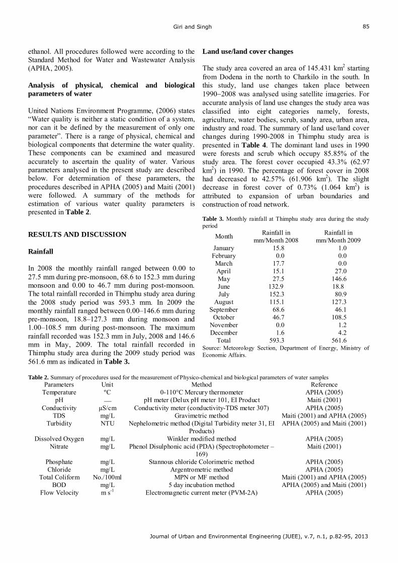
Giri and Singh
Journal of Urban and Environmental Engineering (JUEE), v.7, n.1, p.82-95, 2013
85
ethanol. All procedures followed were according to the Standard Method for Water and Wastewater Analysis (APHA, 2005).
Analysis of physical, chemical and biological parameters of water United Nations Environment Programme, (2006) states “Water quality is neither a static condition of a system, nor can it be defined by the measurement of only one parameter”. There is a range of physical, chemical and biological components that determine the water quality. These components can be examined and measured accurately to ascertain the quality of water. Various parameters analysed in the present study are described below. For determination of these parameters, the procedures described in APHA (2005) and Maiti (2001) were followed. A summary of the methods for estimation of various water quality parameters is presented in Table 2.
RESULTS AND DISCUSSION Rainfall In 2008 the monthly rainfall ranged between 0.00 to 27.5 mm during pre-monsoon, 68.6 to 152.3 mm during monsoon and 0.00 to 46.7 mm during post-monsoon. The total rainfall recorded in Thimphu study area during the 2008 study period was 593.3 mm. In 2009 the monthly rainfall ranged between 0.00–146.6 mm during pre-monsoon, 18.8–127.3 mm during monsoon and 1.00–108.5 mm during post-monsoon. The maximum rainfall recorded was 152.3 mm in July, 2008 and 146.6 mm in May, 2009. The total rainfall recorded in Thimphu study area during the 2009 study period was 561.6 mm as indicated in Table 3.
Land use/land cover changes The study area covered an area of 145.431 km2 starting from Dodena in the north to Charkilo in the south. In this study, land use changes taken place between 19902008 was analysed using satellite imageries. For accurate analysis of land use changes the study area was classified into eight categories namely, forests, agriculture, water bodies, scrub, sandy area, urban area, industry and road. The summary of land use/land cover changes during 1990-2008 in Thimphu study area is presented in Table 4. The dominant land uses in 1990 were forests and scrub which occupy 85.85% of the study area. The forest cover occupied 43.3% (62.97 km2) in 1990. The percentage of forest cover in 2008 had decreased to 42.57% (61.906 km2). The slight decrease in forest cover of 0.73% (1.064 km2) is attributed to expansion of urban boundaries and construction of road network. Table 3. Monthly rainfall at Thimphu study area during the study period
Month Rainfall in mm/Month 2008
Rainfall in mm/Month 2009
January 15.8 1.0 February 0.0 0.0 March 17.7 0.0 April 15.1 27.0 May 27.5 146.6 June 132.9 18.8 July 152.3 80.9
August 115.1 127.3 September 68.6 46.1
October 46.7 108.5 November 0.0 1.2 December 1.6 4.2
Total 593.3 561.6 Source: Meteorology Section, Department of Energy, Ministry of Economic Affairs.
Table 2. Summary of procedures used for the measurement of Physico-chemical and biological parameters of water samples Parameters Unit Method Reference
Temperature ºC 0-110°C Mercury thermometer APHA (2005) pH pH meter (Delux pH meter 101, EI Product Maiti (2001)
Conductivity µS/cm Conductivity meter (conductivity-TDS meter 307) APHA (2005) TDS mg/L Gravimetric method Maiti (2001) and APHA (2005)
Turbidity NTU Nephelometric method (Digital Turbidity meter 31, EI Products)
APHA (2005) and Maiti (2001)
Dissolved Oxygen mg/L Winkler modified method APHA (2005) Nitrate mg/L Phenol Disulphonic acid (PDA) (Spectrophotometer –
169) Maiti (2001)
Phosphate mg/L Stannous chloride Colorimetric method APHA (2005) Chloride mg/L Argentrometric method APHA (2005)
Total Coliform No./100ml MPN or MF method Maiti (2001) and APHA (2005) BOD mg/L 5 day incubation method APHA (2005) and Maiti (2001)
Flow Velocity m s-1 Electromagnetic current meter (PVM-2A) APHA (2005)
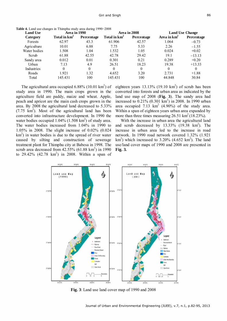
Giri and Singh
Journal of Urban and Environmental Engineering (JUEE), v.7, n.1, p.82-95, 2013
86
Table 4. Land use changes in Thimphu study area during 1990−2008 Area in 1990 Area in 2008 Land Use Change Land Use
Category Total in km2 Percentage Total in km2 Percentage Area in km2 Percentage Forests 62.97 43.3 61.906 42.57 1.064 0.73
Agriculture 10.01 6.88 7.75 5.33 2.26 1.55 Water bodies 1.508 1.04 1.532 1.05 0.024 +0.02
Scrub 61.88 42.55 42.78 29.42 19.1 13.13 Sandy area 0.012 0.01 0.301 0.21 0.289 +0.20
Urban 7.13 4.9 26.51 18.23 19.38 +13.33 Industries 0 0 0 0 0 0
Roads 1.921 1.32 4.652 3.20 2.731 +1.88 Total 145.431 100 145.431 100 44.848 30.84
The agricultural area occupied 6.88% (10.01 km2) of
study area in 1990. The main crops grown in the agriculture field are paddy, maize and wheat. Apple, peach and apricot are the main cash crops grown in the area. By 2008 the agricultural land decreased to 5.33% (7.75 km2). Most of the agricultural land has been converted into infrastructure development. In 1990 the water bodies occupied 1.04% (1.508 km2) of study area. The water bodies increased from 1.04% in 1990 to 1.05% in 2008. The slight increase of 0.02% (0.024 km2) in water bodies is due to the spread of river water caused by silting and construction of sewerage treatment plant for Thimphu city at Babesa in 1998. The scrub area decreased from 42.55% (61.88 km2) in 1990 to 29.42% (42.78 km2) in 2008. Within a span of
eighteen years 13.13% (19.10 km2) of scrub has been converted into forests and urban area as indicated by the land use map of 2008 (Fig. 3). The sandy area had increased to 0.21% (0.301 km2) in 2008. In 1990 urban area occupied 7.13 km2 (4.90%) of the study area. Within a span of eighteen years urban area expanded by more than three times measuring 26.51 km2 (18.23%).
With the increase in urban area the agricultural land and scrub decreased by 13.33% (19.38 km2). The increase in urban area led to the increase in road network. In 1990 road network covered 1.32% (1.921 km2) which increased to 3.20% (4.652 km2). The land use/land cover maps of 1990 and 2008 are presented in Fig. 3.
Fig. 3: Land use land cover map of 1990 and 2008
Giri and Singh
Journal of Urban and Environmental Engineering (JUEE), v.7, n.1, p.82-95, 2013
87
Urbanization in Bhutan began in 1961 with the start of first five year development plan by the late king, Jigme Dorji Wangchuck. Prior to 1961, an urban settlement in Bhutan was limited to a few traditional clustered villages in the valleys. Before 1953, Thimphu had just a dzong (fort) surrounded by a few cluster of traditional houses. The developmental activities in Thimphu started in a rapid pace with its designation as capital of Bhutan by the late king, Jigme Dorji Wangchuck in 1953. The establishment of infrastructural, educational and health facilities attracted job seekers and entrepreneurs. The public sector and private sector expanded quickly to provide various services. This led to the migration of people from rural areas to Thimphu urban area. However, the land availability for urban area is severely limited by the topography.
In 1990 the population of Thimphu urban area was barely 28 012. By 2008 the population of Thimphu urban area increased to over one lakh (National Statistical Bureau, 2008). It is estimated that the population growth rate in Thimphu is 10% per annum. The rapid increase in population caused housing shortage in urban area. This has led to the exponential growth of unauthorized housing in the outskirt of the urban boundary. Starting from 1990, the population of Thimphu urban area increased rapidly.
The expansion of urban area and increase in population in urban area is seen as a worldwide phenomenon. The United States Environmental Protection Agency (USEPA, 2001) report confirmed that every urban area has expanded substantially in land area in recent decades. The percentage of the world’s population living in urban areas was less than 5 percent in 1800, which had increased to 47 percent in 2000 and it is expected to reach 65 percent by 2030 (United Nations Human Development Report, 1990; 1991).
Rao (1991) reported that land available for productive use in India is decreasing in the alarming trend in the per capita availability of arable land from 0.48 ha in 1951 to 0.20 ha in 1981. Sharma et al. (2007) further stated that increase in population pressure and limited productive agriculture land has been the key factor for the conversion of forest land to other uses.
Demirici et al. (2006) analyzed land use changes of Kucukcekmece watershed in Istanbul by using remote sensing and GIS from 1963 to 2005 and found that forest and agriculture land had decreased considerably whereas the industrial and residential areas had increased. Singh et al. (1983) and Rai et al. (1994) reported that the land use/land cover changes from forest to other uses have been widespread in the Himalayan region. Sharma et al. (1992) also stated that agricultural land area had increased considerably over
the past four decades in the Himalayas at the cost of other land uses, particularly forests.
Our results on agricultural land use change are not in line with Klein Goldewijk (2000) who found that in the past 300 years agriculture land and pastureland have increased globally by 460% and 560%, respectively. This may be due to small sample size in the present study and also due to less population pressure in Bhutan compared to other developing countries where food production to meet the requirements of growing population is more extensive as well as intensive. If LULC change for entire country is analyzed, which was beyond the scope of the present study, there is possibility that result on agriculture area may be different from the present study. Bruinsma (2003) also reported that in the developing countries, agriculture land for food production is projected to increase by 13% whereas it is declining in developed countries. It is well known that when LULC changes occur and forest land is converted to other uses, the water regime of the area is altered. Such alterations may be quantitative and/or qualitative, which include deterioration in water quality, increase in volume and velocity of runoff, increase in frequency and severity of flooding, reduction in ground water recharge and perennial flow of streams and rivers, increase in TDS due to erosion etc. (Calder, 2000).
(d) Study on water quality The studies on Physico-chemical and biological parameters were carried out from 2008 to 2009. The physico-chemical parameters of water analysed at upstream, within the urban area and downstream were water temperature, pH, conductivity, total dissolved solids, turbidity, dissolved oxygen, nitrate, phosphate, chloride, sulphate and biochemical oxygen demand. The qualitative and quantitative variations in benthic macro-invertebrates population were also studied. The results are presented separately and sequentially for each parameters studied. The following parameters were assessed to study the water quality in and around Thimphu urban area:
Water Temperature
The minimum water temperature recorded during the study period was 5.88˚C ± 0.47 during post-monsoon of 2009 at sampling site I and the maximum temperature measured was 19.3˚C ± 0.58 during the monsoon of 2008 at sampling site VI. The water temperature increased gradually from sampling site I to VI during pre-monsoon and monsoon. This is because of the altitudinal variations of different sampling sites. Sampling site I in all three study areas are located at the highest altitude whereas Sampling sites VI are at the
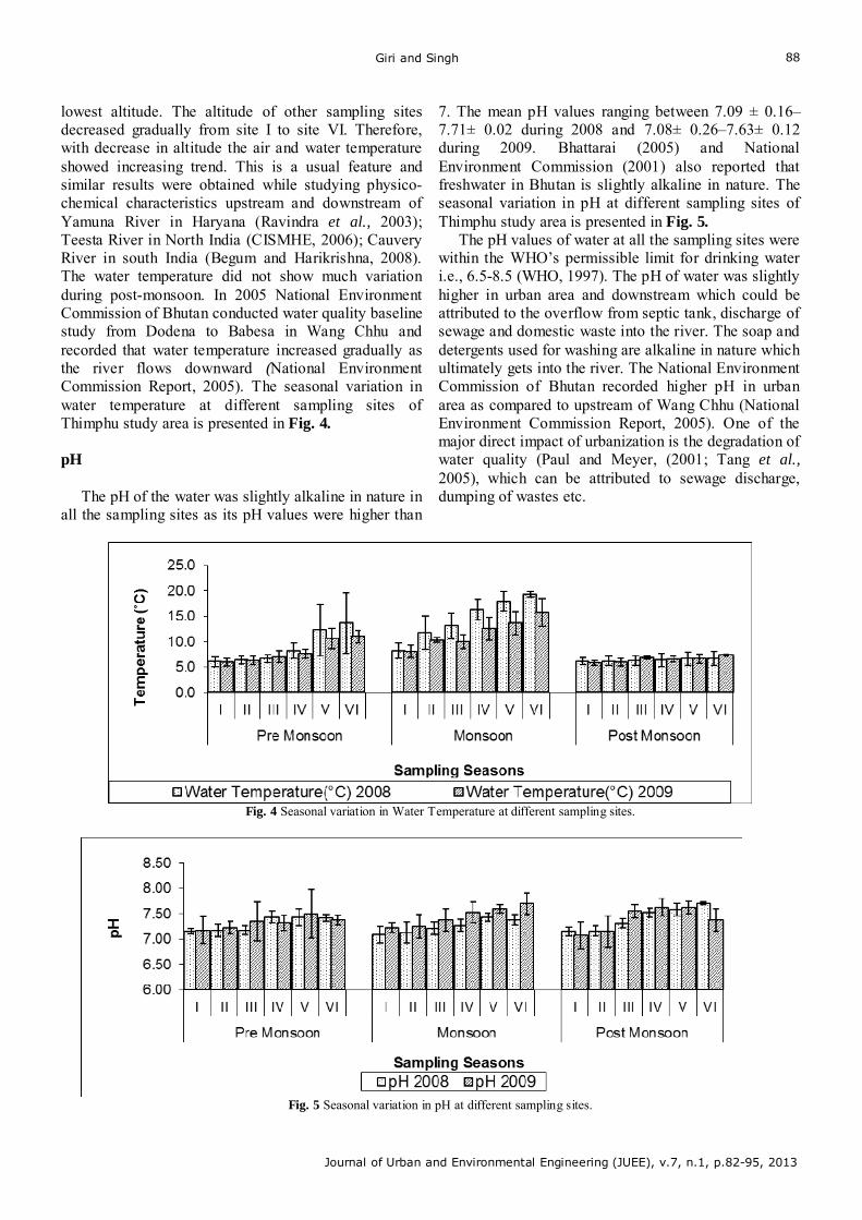
Giri and Singh
Journal of Urban and Environmental Engineering (JUEE), v.7, n.1, p.82-95, 2013
88
lowest altitude. The altitude of other sampling sites decreased gradually from site I to site VI. Therefore, with decrease in altitude the air and water temperature showed increasing trend. This is a usual feature and similar results were obtained while studying physico-chemical characteristics upstream and downstream of Yamuna River in Haryana (Ravindra et al., 2003); Teesta River in North India (CISMHE, 2006); Cauvery River in south India (Begum and Harikrishna, 2008). The water temperature did not show much variation during post-monsoon. In 2005 National Environment Commission of Bhutan conducted water quality baseline study from Dodena to Babesa in Wang Chhu and recorded that water temperature increased gradually as the river flows downward (National Environment Commission Report, 2005). The seasonal variation in water temperature at different sampling sites of Thimphu study area is presented in Fig. 4.
pH
The pH of the water was slightly alkaline in nature in all the sampling sites as its pH values were higher than
7. The mean pH values ranging between 7.09 ± 0.16–7.71± 0.02 during 2008 and 7.08± 0.26–7.63± 0.12 during 2009. Bhattarai (2005) and National Environment Commission (2001) also reported that freshwater in Bhutan is slightly alkaline in nature. The seasonal variation in pH at different sampling sites of Thimphu study area is presented in Fig. 5.
The pH values of water at all the sampling sites were within the WHO’s permissible limit for drinking water i.e., 6.5-8.5 (WHO, 1997). The pH of water was slightly higher in urban area and downstream which could be attributed to the overflow from septic tank, discharge of sewage and domestic waste into the river. The soap and detergents used for washing are alkaline in nature which ultimately gets into the river. The National Environment Commission of Bhutan recorded higher pH in urban area as compared to upstream of Wang Chhu (National Environment Commission Report, 2005). One of the major direct impact of urbanization is the degradation of water quality (Paul and Meyer, (2001; Tang et al., 2005), which can be attributed to sewage discharge, dumping of wastes etc.
Fig. 4 Seasonal variation in Water Temperature at different sampling sites.
Fig. 5 Seasonal variation in pH at different sampling sites.
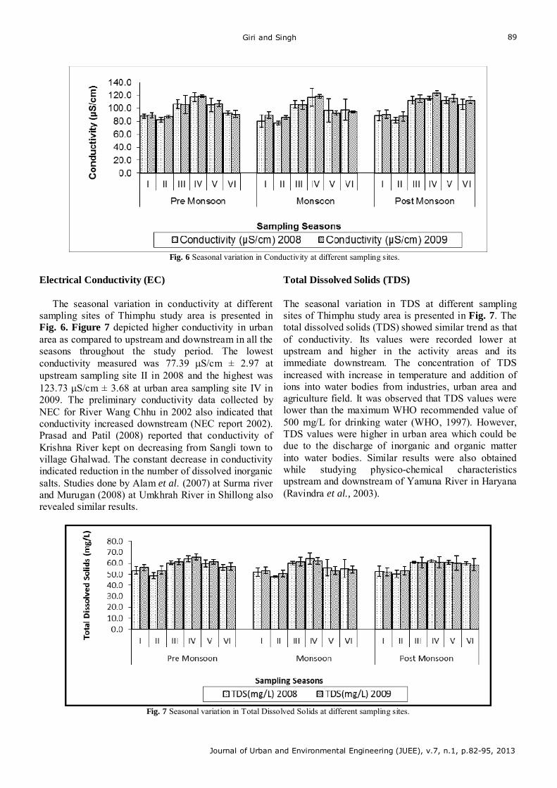
Giri and Singh
Journal of Urban and Environmental Engineering (JUEE), v.7, n.1, p.82-95, 2013
89
Fig. 6 Seasonal variation in Conductivity at different sampling sites.
Electrical Conductivity (EC)
The seasonal variation in conductivity at different sampling sites of Thimphu study area is presented in Fig. 6. Figure 7 depicted higher conductivity in urban area as compared to upstream and downstream in all the seasons throughout the study period. The lowest conductivity measured was 77.39 S/cm ± 2.97 at upstream sampling site II in 2008 and the highest was 123.73 S/cm ± 3.68 at urban area sampling site IV in 2009. The preliminary conductivity data collected by NEC for River Wang Chhu in 2002 also indicated that conductivity increased downstream (NEC report 2002). Prasad and Patil (2008) reported that conductivity of Krishna River kept on decreasing from Sangli town to village Ghalwad. The constant decrease in conductivity indicated reduction in the number of dissolved inorganic salts. Studies done by Alam et al. (2007) at Surma river and Murugan (2008) at Umkhrah River in Shillong also revealed similar results.
Total Dissolved Solids (TDS) The seasonal variation in TDS at different sampling sites of Thimphu study area is presented in Fig. 7. The total dissolved solids (TDS) showed similar trend as that of conductivity. Its values were recorded lower at upstream and higher in the activity areas and its immediate downstream. The concentration of TDS increased with increase in temperature and addition of ions into water bodies from industries, urban area and agriculture field. It was observed that TDS values were lower than the maximum WHO recommended value of 500 mg/L for drinking water (WHO, 1997). However, TDS values were higher in urban area which could be due to the discharge of inorganic and organic matter into water bodies. Similar results were also obtained while studying physico-chemical characteristics upstream and downstream of Yamuna River in Haryana (Ravindra et al., 2003).
Fig. 7 Seasonal variation in Total Dissolved Solids at different sampling sites.
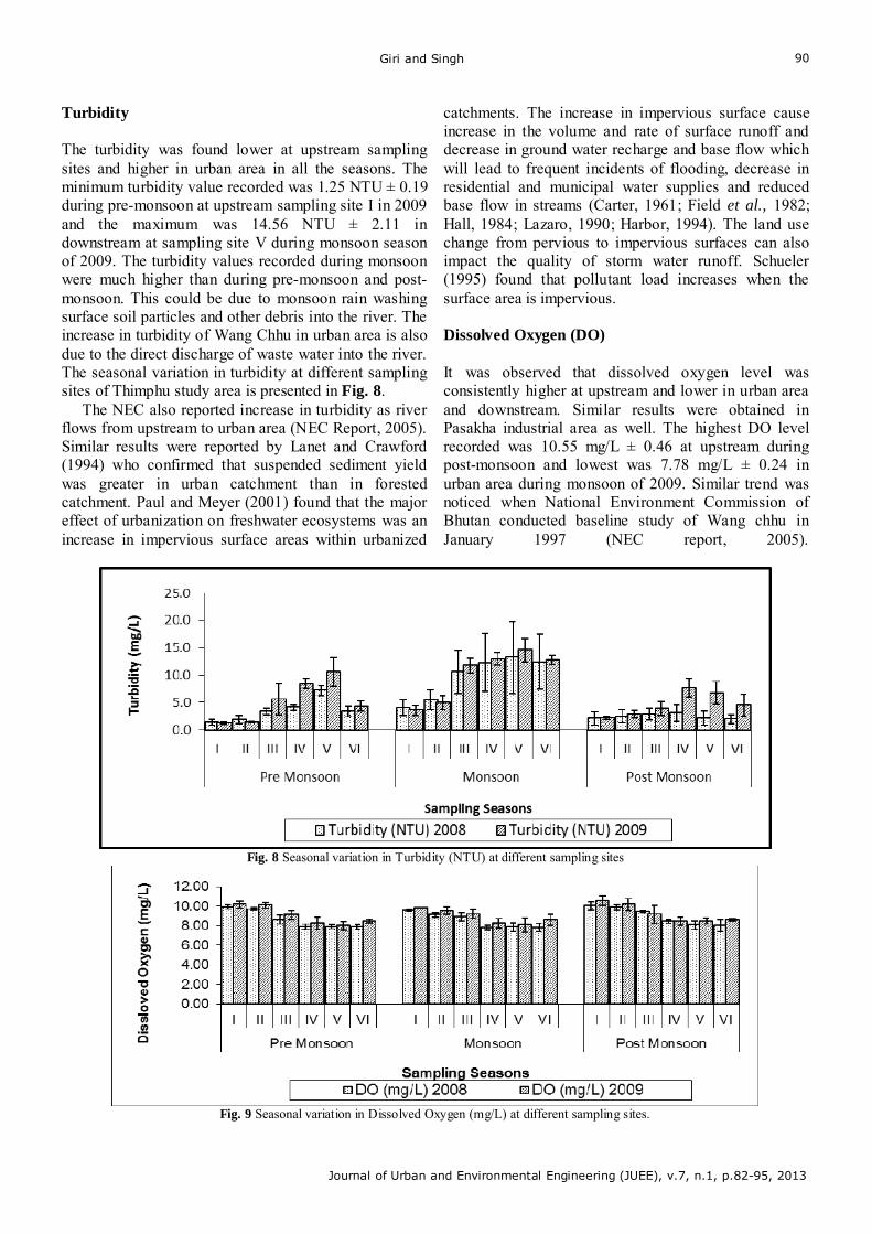
Giri and Singh
Journal of Urban and Environmental Engineering (JUEE), v.7, n.1, p.82-95, 2013
90
Turbidity The turbidity was found lower at upstream sampling sites and higher in urban area in all the seasons. The minimum turbidity value recorded was 1.25 NTU ± 0.19 during pre-monsoon at upstream sampling site I in 2009 and the maximum was 14.56 NTU ± 2.11 in downstream at sampling site V during monsoon season of 2009. The turbidity values recorded during monsoon were much higher than during pre-monsoon and post-monsoon. This could be due to monsoon rain washing surface soil particles and other debris into the river. The increase in turbidity of Wang Chhu in urban area is also due to the direct discharge of waste water into the river. The seasonal variation in turbidity at different sampling sites of Thimphu study area is presented in Fig. 8.
The NEC also reported increase in turbidity as river flows from upstream to urban area (NEC Report, 2005). Similar results were reported by Lanet and Crawford (1994) who confirmed that suspended sediment yield was greater in urban catchment than in forested catchment. Paul and Meyer (2001) found that the major effect of urbanization on freshwater ecosystems was an increase in impervious surface areas within urbanized
catchments. The increase in impervious surface cause increase in the volume and rate of surface runoff and decrease in ground water recharge and base flow which will lead to frequent incidents of flooding, decrease in residential and municipal water supplies and reduced base flow in streams (Carter, 1961; Field et al., 1982; Hall, 1984; Lazaro, 1990; Harbor, 1994). The land use change from pervious to impervious surfaces can also impact the quality of storm water runoff. Schueler (1995) found that pollutant load increases when the surface area is impervious.
Dissolved Oxygen (DO) It was observed that dissolved oxygen level was consistently higher at upstream and lower in urban area and downstream. Similar results were obtained in Pasakha industrial area as well. The highest DO level recorded was 10.55 mg/L ± 0.46 at upstream during post-monsoon and lowest was 7.78 mg/L ± 0.24 in urban area during monsoon of 2009. Similar trend was noticed when National Environment Commission of Bhutan conducted baseline study of Wang chhu in January 1997 (NEC report, 2005).
Fig. 8 Seasonal variation in Turbidity (NTU) at different sampling sites
Fig. 9 Seasonal variation in Dissolved Oxygen (mg/L) at different sampling sites.
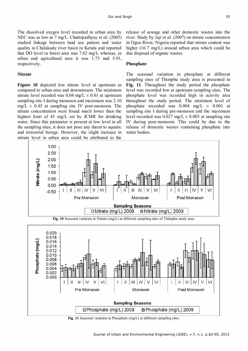
Giri and Singh
Journal of Urban and Environmental Engineering (JUEE), v.7, n.1, p.82-95, 2013
91
The dissolved oxygen level recorded in urban area by NEC was as low as 7 mg/L. Chattopadhyay et al. (2005) studied linkage between land use pattern and water quality in Chalakudy river basin in Kerala and reported that DO level in forest area was 7.62 mg/L whereas, in urban and agricultural area it was 1.73 and 5.91, respectively. Nitrate Figure 10 depicted low nitrate level at upstream as compared to urban area and downstream. The minimum nitrate level recoded was 0.04 mg/L ± 0.01 at upstream sampling site I during monsoon and maximum was 2.10 mg/L ± 0.45 at sampling site IV post-monsoon. The nitrate concentration were found much lower than the highest limit of 45 mg/L set by ICMR for drinking water. Since this parameter is present at low level in all the sampling sites, it does not pose any threat to aquatic and terrestrial beings. However, the slight increase in nitrate level in urban area could be attributed to the
release of sewage and other domestic wastes into the river. Study by Jaji et al. (2007) on nitrate concentration in Ogun River, Nigeria reported that nitrate content was higher (16.7 mg/L) around urban area which could be due disposal of organic wastes. Phosphate The seasonal variation in phosphate at different sampling sites of Thimphu study area is presented in Fig. 11. Throughout the study period the phosphate level was recorded low at upstream sampling sites. The phosphate level was recorded high in activity area throughout the study period. The minimum level of phosphate recorded was 0.004 mg/L ± 0.001 at sampling site I during pre-monsoon and the maximum level recorded was 0.027 mg/L ± 0.003 at sampling site IV during post-monsoon. This could be due to the release of domestic wastes containing phosphate into water bodies.
Fig. 10 Seasonal variation in Nitrate (mg/L) at different sampling sites of Thimphu study area.
Fig. 11 Seasonal variation in Phosphate (mg/L) at different sampling sites.
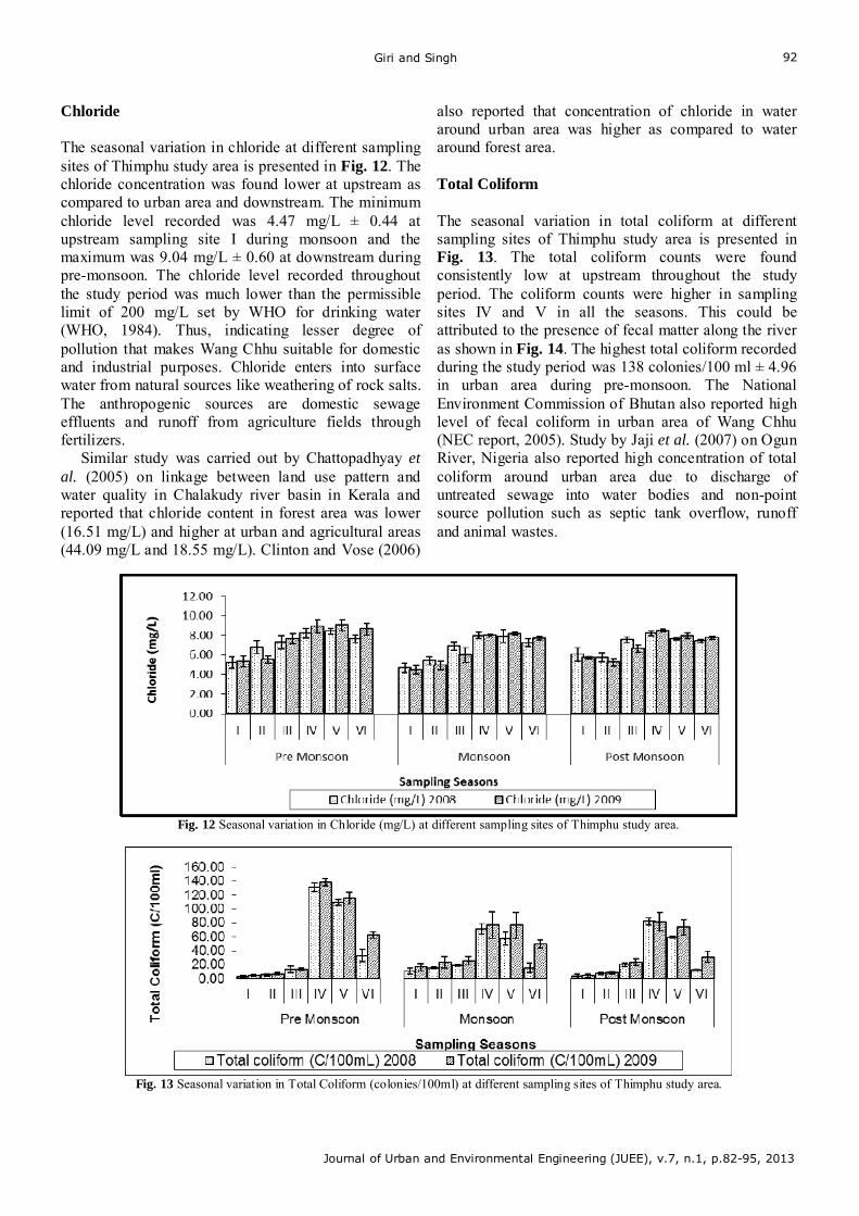
Giri and Singh
Journal of Urban and Environmental Engineering (JUEE), v.7, n.1, p.82-95, 2013
92
Chloride The seasonal variation in chloride at different sampling sites of Thimphu study area is presented in Fig. 12. The chloride concentration was found lower at upstream as compared to urban area and downstream. The minimum chloride level recorded was 4.47 mg/L ± 0.44 at upstream sampling site I during monsoon and the maximum was 9.04 mg/L ± 0.60 at downstream during pre-monsoon. The chloride level recorded throughout the study period was much lower than the permissible limit of 200 mg/L set by WHO for drinking water (WHO, 1984). Thus, indicating lesser degree of pollution that makes Wang Chhu suitable for domestic and industrial purposes. Chloride enters into surface water from natural sources like weathering of rock salts. The anthropogenic sources are domestic sewage effluents and runoff from agriculture fields through fertilizers.
Similar study was carried out by Chattopadhyay et al. (2005) on linkage between land use pattern and water quality in Chalakudy river basin in Kerala and reported that chloride content in forest area was lower (16.51 mg/L) and higher at urban and agricultural areas (44.09 mg/L and 18.55 mg/L). Clinton and Vose (2006)
also reported that concentration of chloride in water around urban area was higher as compared to water around forest area. Total Coliform The seasonal variation in total coliform at different sampling sites of Thimphu study area is presented in Fig. 13. The total coliform counts were found consistently low at upstream throughout the study period. The coliform counts were higher in sampling sites IV and V in all the seasons. This could be attributed to the presence of fecal matter along the river as shown in Fig. 14. The highest total coliform recorded during the study period was 138 colonies/100 ml ± 4.96 in urban area during pre-monsoon. The National Environment Commission of Bhutan also reported high level of fecal coliform in urban area of Wang Chhu (NEC report, 2005). Study by Jaji et al. (2007) on Ogun River, Nigeria also reported high concentration of total coliform around urban area due to discharge of untreated sewage into water bodies and non-point source pollution such as septic tank overflow, runoff and animal wastes.
Fig. 12 Seasonal variation in Chloride (mg/L) at different sampling sites of Thimphu study area.
Fig. 13 Seasonal variation in Total Coliform (colonies/100ml) at different sampling sites of Thimphu study area.
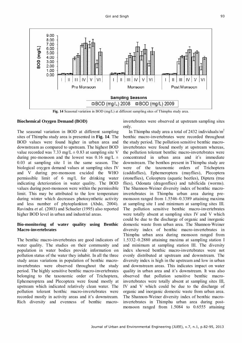
Giri and Singh
Journal of Urban and Environmental Engineering (JUEE), v.7, n.1, p.82-95, 2013
93
Fig. 14 Seasonal variation in BOD (mg/L) at different sampling sites of Thimphu study area.
Biochemical Oxygen Demand (BOD) The seasonal variation in BOD at different sampling sites of Thimphu study area is presented in Fig. 14. The BOD values were found higher in urban area and downstream as compared to upstream. The highest BOD value recorded was 7.33 mg/L ± 0.83 at sampling site V during pre-monsoon and the lowest was 0.16 mg/L ± 0.03 at sampling site I in the same season. The biological oxygen demand values at sampling sites IV and V during pre-monsoon excided the WHO permissible limit of 6 mg/L for drinking water indicating deterioration in water quality. The BOD values during post-monsoon were within the permissible limit. This may be attributed to the low temperature during winter which decreases photosynthetic activity and less number of phytoplankton (Abdo, 2004). Ravindra et al. (2003) and Schueler (1995) also reported higher BOD level in urban and industrial areas.
Bio-monitoring of water quality using Benthic Macro-invertebrates The benthic macro-invertebrates are good indicators of water quality. The studies on their community and population in water bodies provide information on pollution status of the water they inhabit. In all the three study areas variations in population of benthic macro-invertebrates were observed throughout the study period. The highly sensitive benthic macro-invertebrates belonging to the taxonomic order of Trichoptera, Ephemeroptera and Plecoptera were found mostly at upstream which indicated relatively clean water. The pollution tolerant benthic macro-invertebrates were recorded mostly in activity areas and it’s downstream. Rich diversity and evenness of benthic macro-
invertebrates were observed at upstream sampling sites only.
In Thimphu study area a total of 2432 individuals/m2 benthic macro-invertebrates were recorded throughout the study period. The pollution sensitive benthic macro-invertebrates were found mostly at upstream whereas, the pollution tolerant benthic macro-invertebrates were concentrated in urban area and it’s immediate downstream. The benthos present in Thimphu study are were of the taxonomic orders of Trichoptera (caddisflies), Ephemeroptera (mayflies), Plecoptera (stoneflies), Coleoptera (aquatic beetles), Diptera (true flies), Odonata (dragonflies) and tubificida (worms). The Shannon-Weiner diversity index of benthic macro-invertebrates in Thimphu urban area during pre-monsoon ranged from 1.5546–0.3389 attaining maxima at sampling site I and minimum at sampling sites III. The pollution sensitive benthic macro-invertebrates were totally absent at sampling sites IV and V which could be due to the discharge of organic and inorganic domestic waste from urban area. The Shannon-Weiner diversity index of benthic macro-invertebrates in Thimphu urban area during monsoon ranged from 1.5332–0.2880 attaining maxima at sampling station I and minimum at sampling station III. The diversity index showed benthic macro-invertebrates were not evenly distributed at upstream and downstream. The diversity index is high in the upstream and low in urban and downstream areas. This indicates impact on water quality in urban area and it’s downstream. It was also observed that pollution sensitive benthic macro-invertebrates were totally absent at sampling sites III, IV and V which could be due to the discharge of organic and inorganic domestic waste from urban area. The Shannon-Weiner diversity index of benthic macro-invertebrates in Thimphu urban area during post-monsoon ranged from 1.5084 to 0.6555 attaining
Giri and Singh
Journal of Urban and Environmental Engineering (JUEE), v.7, n.1, p.82-95, 2013
94
maximum at sampling site I and minimum at sampling station IV and V. The diversity index showed benthic macro-invertebrates were not evenly distributed at upstream and downstream. The evenness ranged from 0.9826 to 7566 attaining maximum at sampling site III and minimum at sampling site II.
Many studies have reported that benthic communities have good correlations with the water quality changes (Rosenberg and Resh, 1992; Richards and Minshell, 1992; Resh and Jackson, 1993; Resh, 1995; Mason, 1996; Omar et al., 2002). Recently, study done by Duran (2006) found that compared to upper area, lower area had lower diversity of benthic macro-invertebrates at Behzat stream in Turkey which was due to the release of phosphate and nitrogen ions into the stream. Our findings are in line with earlier studies which revealed that a clean and healthy ecosystem support diversity of benthic macro-invertebrates whereas, in dirty and unhealthy ecosystem only a few types of pollution resistant organisms survive. Joshi et al. (2007) reported that species richness depend on abiotic factors like temperature, hardness, pH, dissolved oxygen, chloride and phosphorus which are in line with our study. Budin et al. (2008) stated that river or stream pollution will not just increase water shortage for daily use but also affect the aquatic species richness, diversity and population of sensitive benthic macro-invertebrates such as Ephemeroptera (E), Plecoptera (P) and Trichoptera (T) which live in clean water and prefer unpolluted aquatic ecosystems. In our study we have found maximum EPT population at upstream sampling sites where the water quality is relatively clean. Sharma et al. (2008) studied aquatic insect diversity of Chandrabhaga river, Garhwal Himalayas and reported that density and diversity of aquatic insects decreases with increase in turbidity, water temperature and decrease in dissolved oxygen.
CONCLUSION Based on the results of the present study it can be concluded that there are changes in the LULC due to anthropogenic activities. The forest and agriculture land decreased during 1990-2008 and the urban area increased drastically. Such change in LULC pattern is not healthy from the environment and socio-economic point of views and therefore, is a matter of concern. The LULC changes and associated human activities have deteriorated the water quality in the study areas as evident from low DO, higher electrical conductivity, total hardness, total dissolved solids, turbidity, nitrate, chloride, sulphate, BOD and total coliform, presence of pollution tolerant macro-invertebrates etc.
In summary, the study revealed that all along, Bhutan forest land is decreasing. The development of
urban infrastructure are posing threats to water regime in terms of its quantity and quality. Though the deterioration of water quality is restricted to a few localized areas, the trend is serious and needs proper attention of policy planners and decision makers. Proper treatment of effluents from industries and urban areas are urgently needed to reduce water pollution in such affected areas to check further deterioration of water quality. This present study which is based on a small a area can be considered as an eye opener. However, further studies and in-depth analysis of water quality and its impact on human health and socio-economy in Bhutan is needed for policy planning and implementation.
REFERENCES Abdo, M. H. (2004). Environmental studies on the river Nile at
Damietta branch region, Egypt. Journal of Egypt Academic Society for Environment Development 5(2):85-104.
Alam, Md. J. B., Muyen, Z., Islam, M. R., Islam, S. and Mamun, M. (2007). Water quality parameters along rivers. International Journal of Environmental Science and Technology 4(1):159-167.
American Public Health Association (2003). Standard Method for the Examination of Water and Waste water APHA, AWWA, WPCF (21st) edition, American Public Health Association Inc., Springfield, New York.
Bates, B. C., Kundzewicz, Z. W., Wu, S. and Palutikof, J. P. (eds.) (2008). Climate Change and Water. IPCC Secretariat, Geneva.
Begum, A. and Harikrishna (2008). Study on the quality of water in some streams of Cauvery river. E-Journal of Chemistry 5(2), 377-384.
Bhattarai, S. (2005). Study on limnology of freshwater in diverse lentic habitats of Bhutan. Ph.D. thesis submitted to North-Eastern Hill University, 1-172.
Bruinsma, J. (ed.) (2003). World Agriculture: Towards 2015/2030, an FAO study, Earth scan, London. 51-126.
Budin, K., Jubok, Z., Gabra, D., Abdullah, N. and Ahmed, A. (2008). Effect of water parameters on ephemeroptera abundance in Telipok river, Sabah Malaysia. WSEAS Transactions on Environment and Development 5(4):447–501.
Calder, I. R. (2000). Land use impacts on water resources; Land use and water resources research: 2.1-2.14, viewed at www.venus.co.uk, on 2.3.2011.
Cater, W. R. (1961). Magnitude and frequency of floods in suburban areas. US Geological Survey Professional Paper 424-B:9–11.
Centre for Inter-Disciplinary Studies of Mountain and Hill Environment (2006). Carrying capacity study of Teesta basin in Sikkim, Volume IV, Water environment, Ministry of Environment & Forests, Government of India, 46-65.
Chattopadhyay, S., Rani, L. A. and Sangeetha, P. V. (2005). Water quality variations as linked to land use pattern: a case study in Chalakudy river basin, Kerala. Current Science 89(12), 2163–2169.
Clinton, B. D. and Vose, J. M. (2006). Variation in stream water quality in an urban headwater stream in the southern Appalachians. Water, Air and Soil Pollution 169(3), 331-353.
Demirci, A., Mcadams, M. A., Alagha, O. and Karakuyu, M. (2006). The relationship between land use change and water quality in Kucukcekmece lake watershed. Retrived on 15.5.2010 from http://dis.fatih.edu.tr/store/does/970940/TWZQ2sk.pdf.
Duran, M. (2006). Monitoring water quality using benthic macroinvertebrates and physico-chemical parameters of Behzat
Giri and Singh
Journal of Urban and Environmental Engineering (JUEE), v.7, n.1, p.82-95, 2013
95
stream in Turkey. Polish Journal of Environmental Studies 15(5), 709–717.
Hall, M. J. (1984). Urban Hydrology: Elsevier applied science publishers, New York, 1-115.
Harbor, J. (1994). A practical method for estimating the impact of land use change on surface runoff, groundwater recharge and wetland hydrology. Journal of American Planning Association 60(1), 91–104.
Joshi, P. C., Kumar, K., Badoni, V., and Singh, A. (2002). An ecological study on the above ground entomofauna of Nanda Devi biosphere reserve in Sharma, J. K., Easa, P. S., Mohanan, C., Sasidhara, N. and Rai, R. K. (eds.) Biosphere reserves in India and their management: Ministry of Environment and Forest, Government of India. New Delhi, 143-149.
Klein Goldewijk, K. (2000). Estimating global land use change over the past 300 years: The HYDE Database. In: Global Biogeochemical Cycles 15(4), 417–433.
Lazaro, T. R. (1990). Urban Hydrology, a Multidisciplinary Perspective: Technomic publishing company, Lancaster, 21-36.
Lenat, D. R. and Crawford, J. K. (1994). Effects of land use on water quality and aquatic biota of three North Carolina Piedmont streams. Hydrobiologia 294(3):185-199.
Maite, S. K. (2001). Handbook of Methods in Environmental Studies Vol. I – Water and wastewater analysis: ABD Publishers, Jaipur, India.
Mason, C. F. (1996). Biology of Freshwater Pollution: Longman, New York, 8-19.
Murugan, A. (2008). Physico-chemical properties of water quality of river Umkhrah, Shillong, Meghalaya. Journal of Basic and Applied Biology 2(1):94–98.
National Environment Commission (2001). Bhutan: State of Environment, Royal Government of Bhutan, Thimphu.
National Environment Commission (2002). National Environment Commission Report, NEC, Thimphu.
National Environment Commission (2005). State of Environment Report, National environment Commission, Thimphu.
Organisation for Economic Co-operation and Development (2008). Environmental Outlook to 2030: Organisation for Economic Co-operation and Development, Paris, 21-34.
Paul, M. J. and Meyer, J. L. (2001). Streams in the urban landscape. Annual Review Ecology Systematics 32: 333-365.
Pennack, R. W. (1953) Freshwater invertebrates of the United State: The Roland press company, New York, 34-38.
Pennack, R. W. (1978). Freshwater Invertebrates of United States: John Wiley and Sons, New York.
Prasad, N. R. and Patil, J. M. (2008). A study of physico-chemical parameters of Krishna river water particularly in western Maharashtra. Rasayan J. Chemistry 1(2), 943-958.
Rai, S. C., Sharma, E. and Sundriyal, R. C. (1994). Conservation in the Sikkim Himalaya: traditional knowledge and land-use of the Mamlay watershed. Environmental Conservation 21: 30-34.
Rao, J. R. (2001). Biological resources of the Ganga river, India. Hydrobiologia 458:159-168.
Ravindra, K., Meenakshi, A., Rani, M. and Kaushik, A. (2003). Seasonal variations in physico-chemical characteristics of river Yamuna in Harayana and its ecological best designated use. J. Environmental Monitoring 5(4), 419-426.
Resh, V. H. (1995). Freshwater benthic macroinvertebrates and rapid assessment procedures for water quality monitoring and developing in newly industrialized countries in Davis, W. S. (ed.) Biological Assessment and Criteria: Lewis publishers, England, 167-177.
Resh, V. H. and Jackson, J. K. (1993). Rapid assessment approaches to biomomntoring using benthic macroinvertebrates in Rosenberg, D. M. (ed.) Freshwater biomonitoring and Benthic Macroinvertebrates: kluwer London, UK, 195-233.
Richards, C. and Minshell, G. W. (1992). Spatial and temporal trends in stream macroinvertebrate species assemblages: The influence of watershed disturbance. Hydrobiologia 241(2), 173–184.
Rosenberg, D. M. and Resh, V. H. (1993). Freshwater Biomonitoring and Benthic Macroinvertebrates: Chapman and Hall, New York.
Schueler, T. (1995) Site planning for urban stream protection, Centre for watershed protection, USA.
Sharma E., Sundriyal, R.C., Rai, S.C., Bhatt, Y. K., Rai, L.K., Sharma, R. and Rai, Y.K. (1992). Integrated watershed management: Gyanondays Prakashan Nainital, India.
Sharma, A., Sharma, R.C. and Anthwal, A. (2008). Surveying of aquatic insect diversity of Chandrabhaga river, Garhwal Himalayas. Enviromentalist 28(3), 395-404.
Sharma, R., Xu, J. and Sharma, J. (2007). Traditional agroforestry in the Eastern Himalayan region: land management system supporting ecosystem services. Journal of Tropical Ecology 48(2), 189-200.
Singh, J. S., Pandey, A. N. and Pathak, P. C. (1983). A hypothesis to account for the major pathways of soil loss from Himalaya. Environmental Conservation 10(3), 343-345.
Tang, Z., Engel, B. A., Pijanowski, B. C., and Lim, K. J. (2005). Forecasting land use change and its environmental impact at a watershed scale. Journal of Environmental Management 7691), 35-45.
Thorp, J. H. and Kovich, A. P. (1991). Ecology and Classification of North American Freshwater Invertebrates: Academic Press, United States of America.
United Nations (1990). Human Development Report: Oxford University Press, 30-150.
United Nations Environment Programme (2009). Persistent organic pollutants. Retrieved on 13.10.2009 from http://www.chem.unep.ch/pops/.
United Nations Environment Programme (2009). United Nations Environment Programme Year Book 2009. Nairobi, 5-10.
United Nations Environment programme (2006). Water quality for ecosystem and human health, Ontario, Canada, United Nations Environment programme. Global Environment Monitoring System (GEMS) water Programme, 3-59.
United Nations World Water Assessment Programme (2003). United Nations World Water Development Report: Water for People, Water for Life: UNESCO, Paris, 1-19.
United Nations World Water Assessment Programme (2009). United Nations World Water Assessment Programme. The World Water Development Report 3: Water in a changing world. UNESCO: Paris, France. Retrieved on 12.1.2010 from http://www.unesco.org/water/wwap/wwdr/wwdr3.
United States Environmental Protection Agency (2001). Our built and natural environment: a technical review of the interactions between land use, transportation and environmental quality, 4.
Ward, H. B. and Whipple, G. C. (1992). Freshwater Biology, 2nd edition. Edmondso, W. T. (ed.) International books and periodicals supply service, New Delhi, 1-60.
World Health Organization (1997). Guidelines for Drinking Water Quality, Volume 3, World Health Organization, Geneva, 51-72.
Amoateng, Cobbinah and Owusu-Adade
Journal of Urban and Environmental Engineering (JUEE), v.7, n.1, p.96-109, 2013
96
Journal of Urban and Environmental Engineering, v.7, n.1, p.96-109
Journal of Urban and Environmental Engineering
UEEJ ISSN 1982-3932
doi: 10.4090/juee.2013.v7n1.096109 www.journal-uee.org
MANAGING PHYSICAL DEVELOPMENT IN PERI-URBAN AREAS OF KUMASI, GHANA: A CASE OF ABUAKWA
Paul Amoateng1, Patrick B. Cobbinah1 and Kwasi Owusu-Adade2
1School of Environmental Sciences, Institute for Land, Water and Society, Charles Sturt University, Australia 2Department of Planning, College of Architecture and Planning, Kwame Nkrumah University of Science and
Technology, Ghana
Received 17 September 2012; received in revised form 28 March 2013; accepted 13 April 2013
Abstract: A remarkable trait of the 21st century has been the high rate of urbanization which has
characterized the growth and development of cities especially in developing countries. This situation has fuelled rapid physical development and expansion of peri-urban areas as urban dwellers relocate to cities’ peripheries. Focusing on Abuakwa a peri-urban area in Kumasi, the second largest city in Ghana, this paper assesses the nature and extent of physical development in peri-urban areas, and identifies the factors contributing to the rapid development of peri-urban areas. The paper further examines the effects of the increasing physical growth on the development of peri-urban Abuakwa. Using a case study approach, both primary and secondary sources of data were collected from decentralized government institutions of Kumasi Metropolitan Assembly (KMA) and Atwima Nwabiagya District Assembly (ANDA), as well as indigenes and relocated urban dwellers in Abuakwa. The paper reveals that the outward drift has manifested itself in an increased scramble for land for residential and commercial purposes in the peri-urban area. The resultant effect has been the fast and spontaneous physical development in the urban periphery which has significantly altered the peri-urban morphology. The paper recommends the establishment of Customary Land Secretariat (CLS) to co-ordinate allocation of land, and the application of settlement growth management approaches to ensure the creation of a functional city and liveable peri-urban areas.
Keywords:
Abuakwa; land use; peri-urban areas; physical development
© 2013 Journal of Urban and Environmental Engineering (JUEE). All rights reserved.
Correspondence to: Paul Amoateng, Tel.: +61 0451030256, P.O Box 789, Albury NSW 2460, Australia. E-mail: [email protected]
Amoateng, Cobbinah and Owusu-Adade
Journal of Urban and Environmental Engineering (JUEE), v.7, n.1, p.96-109, 2013
97
INTRODUCTION
The 2010 Population and Housing Census of Ghana indicate that the proportion of urban population in Ghana increased from 43.8 percent in 2000 to 50.9 percent in 2010 (Ghana Statistical Service (GSS), 2012). This high rate of urbanization has accelerated the demand for land to meet the increasing needs of urban dwellers particularly in the major cities in Ghana. As a result, there is seemingly rapid expansion of peri-urban areas where basic facilities such as piped water, electricity and sewage services are virtually non-existent.
These peri-urban areas are characterized by fast and unplanned physical growth and development. The unregulated pattern of physical development in these areas has given rise to complex organic urban growth which predominantly expands horizontally. Explaining this phenomenon, Drabkin (1977) asserts that urban population growth is mainly occurring in the outlying regions of the metropolitan areas due to the engulfment of the peri-urban areas by ‘parent city’. As a result, peri-urban physical development pattern is always undergoing transformation especially in cities in the developing world (Drabkin, 1977). Concomitantly, these dynamic changes in the land use also occur following improvement in accessibility, natural increase in population, presence of serene living environment, and availability of vast but low cost land.
In the context of Kumasi, this phenomenon is ostensibly evident. With an annual population growth rate of 5.4 percent, Kumasi is considered the fastest growing city in Ghana (Cobbinah & Amoako, 2012). The growing population of the city coupled with the availability of infrastructure and relatively low land values at the peripheries has resulted in the inefficient use and over exploitation of natural resources especially land at the outskirts. The city’s peripheries have become the preferred places for housing, industrial and commercial development due to the relatively low land values. As a consequence, the peri-urban areas of Kumasi are experiencing intensive and continuous physical development in an uncontrolled manner. Prime agricultural lands in these areas have been utilized for physical development purposes. However, this uncontrolled pattern of physical development poses urban management challenges to the peri-urban economy, traffic generation and management, growth management, and the provision of ancillary services.
This paper investigates the management of physical development in peri-urban areas of Kumasi by examining the nature and extent of physical development in Abuakwa. It explores the factors contributing to the increasing physical development in and the effects on the development of peri-urban
Abuakwa. The paper concludes with recommendations to ensure efficient and effective management of physical development in peri-urban areas of Kumasi.
CHARACTERISTICS OF PERI-URBAN AREAS AND PHYSICAL DEVELOPMENT
The meaning and characteristics of peri-urban areas
According to Organisation for Economic Co-operation and Development (OECD) (2007) the term ‘peri-urban’ came into public domain and use during the 1980s in Europe. The OECD described peri-urban as a name given to the ‘grey area’ which is neither entirely urban nor rural in the traditional sense. It is neither fully urbanized nor completely rural, but often seen as a ‘middle band’ of land with atypical characteristics (Buxton, 2007). It comprises an unbalanced mixture of urban and rural functions.
Peri-urban area serves as the zone where urban-rural interaction is at its peak (Johnson, 1974). At this zone, rural activities and modes of life are in rapid retreat, with extensive urban land use intrusion (that is urban area physically and functionally expands into the rural area).
Peri-urban areas exhibit peculiar characteristics that make them distinct from urban and rural areas, and these include accelerated development of urban residential and urban commercial uses, and decrease in rural primary activities (Hewitt, 1989), rapid but unplanned growth with inadequate service infrastructure (Government of Swaziland, 1997), middle and low income residents (Johnson, 1974), and serve as receptacles for the growing rental market (Buxton, 2007).
Generally, peri-urban areas can be classified into four interrelated categories. These include village peri-urban, diffused peri-urban, in-place peri-urban and absorbed peri-urban (Drescher & Iaquinta, 2000). The categorization is derived from the underlying socio-demographic processes, especially migration. The defining features connected the elements of the typology in the form of a continuum. The concept of physical development
Keeble (1969) explains physical development as the carrying out of building, engineering, mining or other operations in, on, over or under land or the making of any material or substantial change in the use of any building or land. Physical development entails the carrying out of any operation on or any modification to land by mankind in an attempt to create a liveable and comfortable environment. The ultimate objective of
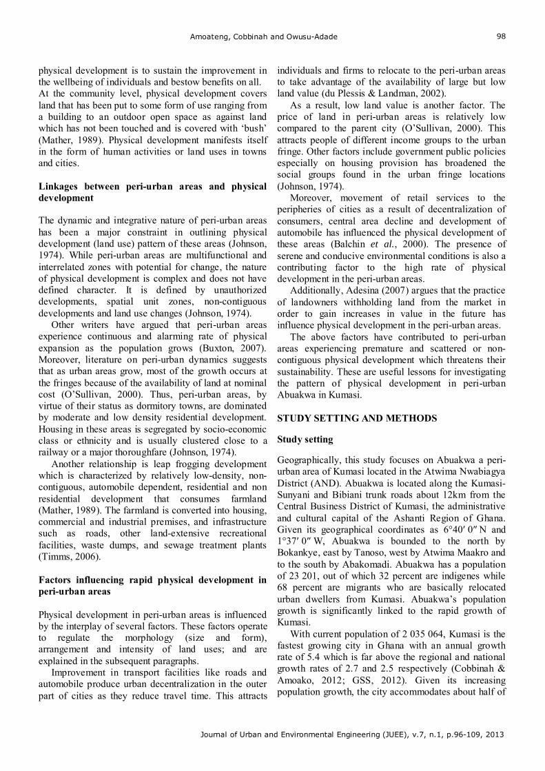
Amoateng, Cobbinah and Owusu-Adade
Journal of Urban and Environmental Engineering (JUEE), v.7, n.1, p.96-109, 2013
98
physical development is to sustain the improvement in the wellbeing of individuals and bestow benefits on all. At the community level, physical development covers land that has been put to some form of use ranging from a building to an outdoor open space as against land which has not been touched and is covered with ‘bush’ (Mather, 1989). Physical development manifests itself in the form of human activities or land uses in towns and cities. Linkages between peri-urban areas and physical development
The dynamic and integrative nature of peri-urban areas has been a major constraint in outlining physical development (land use) pattern of these areas (Johnson, 1974). While peri-urban areas are multifunctional and interrelated zones with potential for change, the nature of physical development is complex and does not have defined character. It is defined by unauthorized developments, spatial unit zones, non-contiguous developments and land use changes (Johnson, 1974).
Other writers have argued that peri-urban areas experience continuous and alarming rate of physical expansion as the population grows (Buxton, 2007). Moreover, literature on peri-urban dynamics suggests that as urban areas grow, most of the growth occurs at the fringes because of the availability of land at nominal cost (O’Sullivan, 2000). Thus, peri-urban areas, by virtue of their status as dormitory towns, are dominated by moderate and low density residential development. Housing in these areas is segregated by socio-economic class or ethnicity and is usually clustered close to a railway or a major thoroughfare (Johnson, 1974).
Another relationship is leap frogging development which is characterized by relatively low-density, non-contiguous, automobile dependent, residential and non residential development that consumes farmland (Mather, 1989). The farmland is converted into housing, commercial and industrial premises, and infrastructure such as roads, other land-extensive recreational facilities, waste dumps, and sewage treatment plants (Timms, 2006).
Factors influencing rapid physical development in peri-urban areas Physical development in peri-urban areas is influenced by the interplay of several factors. These factors operate to regulate the morphology (size and form), arrangement and intensity of land uses; and are explained in the subsequent paragraphs.
Improvement in transport facilities like roads and automobile produce urban decentralization in the outer part of cities as they reduce travel time. This attracts
individuals and firms to relocate to the peri-urban areas to take advantage of the availability of large but low land value (du Plessis & Landman, 2002).
As a result, low land value is another factor. The price of land in peri-urban areas is relatively low compared to the parent city (O’Sullivan, 2000). This attracts people of different income groups to the urban fringe. Other factors include government public policies especially on housing provision has broadened the social groups found in the urban fringe locations (Johnson, 1974).
Moreover, movement of retail services to the peripheries of cities as a result of decentralization of consumers, central area decline and development of automobile has influenced the physical development of these areas (Balchin et al., 2000). The presence of serene and conducive environmental conditions is also a contributing factor to the high rate of physical development in the peri-urban areas.
Additionally, Adesina (2007) argues that the practice of landowners withholding land from the market in order to gain increases in value in the future has influence physical development in the peri-urban areas.
The above factors have contributed to peri-urban areas experiencing premature and scattered or non-contiguous physical development which threatens their sustainability. These are useful lessons for investigating the pattern of physical development in peri-urban Abuakwa in Kumasi.
STUDY SETTING AND METHODS
Study setting Geographically, this study focuses on Abuakwa a peri-urban area of Kumasi located in the Atwima Nwabiagya District (AND). Abuakwa is located along the Kumasi-Sunyani and Bibiani trunk roads about 12km from the Central Business District of Kumasi, the administrative and cultural capital of the Ashanti Region of Ghana. Given its geographical coordinates as 6°40′ 0″ N and 1°37′ 0″ W, Abuakwa is bounded to the north by Bokankye, east by Tanoso, west by Atwima Maakro and to the south by Abakomadi. Abuakwa has a population of 23 201, out of which 32 percent are indigenes while 68 percent are migrants who are basically relocated urban dwellers from Kumasi. Abuakwa’s population growth is significantly linked to the rapid growth of Kumasi.
With current population of 2 035 064, Kumasi is the fastest growing city in Ghana with an annual growth rate of 5.4 which is far above the regional and national growth rates of 2.7 and 2.5 respectively (Cobbinah & Amoako, 2012; GSS, 2012). Given its increasing population growth, the city accommodates about half of
Amoateng, Cobbinah and Owusu-Adade
Journal of Urban and Environmental Engineering (JUEE), v.7, n.1, p.96-109, 2013
99
the entire population of the Ashanti region which has facilitated the spread of development into the neighbouring districts (GSS, 2012).
As a consequence, peri-urban Abuakwa has strong physical and functional links with Kumasi, the second largest city in Ghana. This is based on the fact that about 60 percent of the working population of Abuakwa commutes to and from Kumasi daily to engage in socio-economic activities (ANDA, 2006). Owing to its strong relationship with Kumasi, Abuakwa has developed to become one of the major dormitory towns of Kumasi although other commercial and industrial developments or activities have sprung up.
Highlighting the influence of Kumasi, peri-urban Abuakwa is the largest town in the district with an annual growth rate of 9.6 percent (National Development Planning Commission (NDPC), 2004). Abuakwa is currently experiencing extensive physical development which has spread to engulf surrounding communities like Dadease, Apemhase, Kagyase and Arkosah Township. In relation to its spatial structure, Abuakwa has a sector-like or wedge-like morphology due its growth along the two major roads (see Fig. 2).
Despite the high rate of population growth, Abuakwa’s physical development over the past two decades has been sporadic and uncontrolled leading to haphazard and unauthorized physical development pattern with little or no room for both vehicular and pedestrian circulation. Figure 1 shows the location of Abuakwa in relation to the Kumasi metropolis.
Fig. 1 Abuakwa in Kumasi Metropolitan Context. Source: Owusu-Ansah and O’Connor (2006).
Study Methods This paper is based on a study conducted in 2010 on the pattern of physical development in peri-urban areas of Kumasi. Recent data (2012) on the dynamics of physical development in peri-urban areas of Kumasi have been incorporated. Regarding the method used, the study reviewed relevant and related literature on the characteristics of peri-urban areas and physical
development from both developed and developing countries. The literature review was carried out at two levels: global and local. Whereas the global literature review focused on books and journal articles on the concepts, types and characteristics of peri-urban areas and physical development, the local review examined documents including district development plans, physical development reports and town planning schemes used in monitoring socio-economic and physical development of the study area.
Additionally, the study reviewed other documents such as quarterly and annual reports as well as consultancy reports from some of the decentralized government institutions of KMA and ANDA such as the Urban Roads Department, Building Inspectorate Division and the Town and Country Planning Department (TCPD). The review of these documents was critical in establishing the trends of peri-urban developments in Kumasi, and further identified the major stakeholders involved in managing the physical development in the peri-urban areas of Kumasi. This process served as a useful ground in determining the selection of the case study area and the type of institutions and category of respondents to be involved in the study. Ideally, the study intended to cover two peri-urban areas in Kumasi. However, due to unique characteristics of Abuakwa: high population growth rate, its location in different district, availability of data, and physical development challenges, coupled with relatively slow growth rate, and land ownership challenges characterizing the other peri-urban areas, the study was limited to Abuakwa.
Using semi-structured interviews, six institutions were purposively selected to provide data regarding the pattern of physical development in peri-urban areas of Kumasi particularly Abuakwa. These institutions included the TCPD in Kumasi and ANDA, Building Inspectorate Division of KMA and ANDA, Urban Roads Department of KMA and the Feeder Roads Department of ANDA. The semi-structured interviews allowed for detailed assessment of the phenomena being investigated into (Sarantakos, 1998), and further offered sufficient flexibility to approach different institutions differently while still covering the same areas of data collection (Mohd Noor, 2008). Moreover, traditional authorities and plot allocation committee in the various suburbs of Abuakwa were interviewed to gain first hand data on the state and direction of physical development in peri-urban Abuakwa.
With a total housing stock of 1630, a total of 143 house owners comprising indigenes and relocated urban dwellers were selected and involved in the study using structured questionnaires. The determination of the sample size was done employing the following mathematical model: n= N/1+N (α)2 (Miller & Brewer,
Amoateng, Cobbinah and Owusu-Adade
Journal of Urban and Environmental Engineering (JUEE), v.7, n.1, p.96-109, 2013
100
B APT IST SEMINARY
ABUA KWA FORM ULATIONPLANT
PLAZA
L PMKTTO NKAWIE
TO SUNYANI
ASENEMASO
TANOSO
AGOGOABAKOMADI
NSONYAMEYE
RESIDENTIAL
COMMERCIAL
EDUCATION
OPEN SPACE
CIVIC & CULTURE
SANITATION
UNDEVELOPEDLAND
CIRCULATION
N
SCALE: 1:5,000
GARAGEHOTEL
LEGEND
FROM KUMASI
BOKANKYE
RIVER
CLINIC
INDUSTRY
DIRECTION OF GROWTH
Fig. 2 State of Physical Development in Abuakwa (1993).
Source: Town and Country Planning Department, ANDA
CLINIC
BAPTIST SEMINARY
F R
PLAZA
ABUAKWA FORMULATION PLANT
CEM
GARAGE
MKT L P
HOTEL
CEM
TO NKAWIE
TO SUNYANI
ASENEMASO
TANOSO
AGOGOABAKOMADI
NSONYAMEYE
FROM KUMASI
BOKANKYE
RESIDENTIAL
COMMERCIAL
EDUCATION
OPEN SPACE
CIVIC & CULTURE
SANITATION
UNDEVELOPEDLAND
CIRCULATION
N
SCALE: 1:5,000
RIVER
LEGEND
MIXED USE
INDUSTRY
DIRECTION OF GROWTH
Fig. 3 The Extent and Nature of Physical Development in Abuakwa (2010).
Amoateng, Cobbinah and Owusu-Adade
Journal of Urban and Environmental Engineering (JUEE), v.7, n.1, p.96-109, 2013
101
2003), where n is the sample size, N is the total housing stock (sample frame) and α is the margin of error (0.08). The interactions at both institutional and community levels revealed the major factors and manifestations of physical development as well as the effects of rapid physical development on the development of Abuakwa.
The data collected were analyzed using quantitative and qualitative methods. Statistical Package for Social Sciences (SPSS) was used to facilitate the quantitative analysis while the qualitative analysis focused on description and explanation of the pattern of peri-urban development. The SPSS facilitated the analysis process by generating descriptive statistics such as percentages and frequency counts as well as establishing relationships between study variables (peri-urban areas and physical development).
To ensure the validity and reliability of the study findings, data collected from both the institutional and community levels were harmonized and findings presented to stakeholders at the institutional and local levels. This process proved useful in addressing any gaps and inconsistencies that had occurred.
RESULTS AND DISCUSSIONS Physical growth and expansion of Abuakwa Until 1993, physical development in Abuakwa just like many other peri-urban areas in Ghana was not guided by planning scheme. This is because such areas had not been zoned as planning areas under the Town and Country Planning Ordinance of 1945, (CAP 84) which was the legal framework for regulating planning activities in the country then. The study revealed that physical development prior to 1993 was mainly concentrated in the core area and it occurred haphazardly. Following the enactment of the Local Government Act, 1993 (Act 462) which declared all settlements in Ghana, both urban and rural, as planning areas, a planning layout was prepared to control and guide the growth of Abuakwa.
In relation to its spatial changes, the study results show that the town which covered a total land area of 1.7 km2 (432 acres) in 1993 has expanded to a physical size of 4.6 km2 (1,145 acres) in 2010 (see Figs 2 and 3). The town experienced a change of 713 acres in land area, representing 165.0 percent change in size. This indicates that the size of the settlement tripled in less than two decades.
The rapid rate of physical development that has characterized Abuakwa over the last two decades is reflected in the ages of the buildings. Survey results indicated that more than 90 percent of houses in Abuakwa are less than 20 years old, indicating that the
town has witnessed rapid physical development in recent times. Despite the introduction of planning scheme for the town since the 1993, physical development continues to occur in haphazard and uncoordinated manner. As a result, the rapid physical development has outstripped the ability of development control institutions to monitor and regulate it. The current state (2010) of Abuakwa is presented in Fig. 3.
The survey showed that the physical expansion of Abuakwa has not spared the areas which are earmarked as unbuildable areas. Physical development has spread and encroached on ecologically sensitive areas such as rivers, streams, waterlogged areas and open spaces (see Fig. 4). Developers (house owners) disregard the likely negative socio-environmental consequences such as flooding, spread of water related diseases and extinction of the natural habitats. Figure 4 shows a building in a water way in Abuakwa.
The study further unearthed that virtually none of the areas earmarked for ancillary land uses like education, public open space, sanitary areas among others have been utilized for such purposes. Most of such areas have been converted into residential use as a result of non-adherence to planning regulations, uncoordinated land allocation by the traditional leaders (chiefs) and weak enforcement mechanisms. The cumulative effect of this is the current pattern of physical development which can be described as “monotonous development” dominated by residential buildings (shelter zone). Land use inventory of Abuakwa (19932010) The major land use types identified in Abuakwa clearly show its transitional nature from rural to urban. During the land use/physical survey, the following land uses were identified; residential, commercial, industrial, open space, educational, civic and cultural, sanitation, circulation (road network), mixed uses and undeveloped land as presented in Table 1. The total planning land area of Abuakwa is 1,120 acres. These land uses are discussed in the subsequent sub sections. Residential land use The residential land use covers the largest land area and it comprises of all types of housing and cuts across all areas of the town. The residential area which covered a total area of 230 acres representing 20.6 percent in 1993 increased to 702 acres representing to 62.7 percent of the total land area in 2010.
The dominance of residential zone is a manifestation of Abuakwa’s status as a commuters’ residential zone within a system of settlements and a dormitory town for workers of Kumasi.
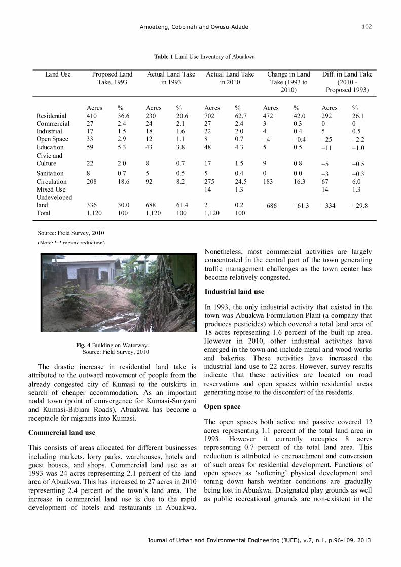
Amoateng, Cobbinah and Owusu-Adade
Journal of Urban and Environmental Engineering (JUEE), v.7, n.1, p.96-109, 2013
102
Fig. 4 Building on Waterway.
Source: Field Survey, 2010
The drastic increase in residential land take is attributed to the outward movement of people from the already congested city of Kumasi to the outskirts in search of cheaper accommodation. As an important nodal town (point of convergence for Kumasi-Sunyani and Kumasi-Bibiani Roads), Abuakwa has become a receptacle for migrants into Kumasi. Commercial land use This consists of areas allocated for different businesses including markets, lorry parks, warehouses, hotels and guest houses, and shops. Commercial land use as at 1993 was 24 acres representing 2.1 percent of the land area of Abuakwa. This has increased to 27 acres in 2010 representing 2.4 percent of the town’s land area. The increase in commercial land use is due to the rapid development of hotels and restaurants in Abuakwa.
Nonetheless, most commercial activities are largely concentrated in the central part of the town generating traffic management challenges as the town center has become relatively congested. Industrial land use In 1993, the only industrial activity that existed in the town was Abuakwa Formulation Plant (a company that produces pesticides) which covered a total land area of 18 acres representing 1.6 percent of the built up area. However in 2010, other industrial activities have emerged in the town and include metal and wood works and bakeries. These activities have increased the industrial land use to 22 acres. However, survey results indicate that these activities are located on road reservations and open spaces within residential areas generating noise to the discomfort of the residents. Open space The open spaces both active and passive covered 12 acres representing 1.1 percent of the total land area in 1993. However it currently occupies 8 acres representing 0.7 percent of the total land area. This reduction is attributed to encroachment and conversion of such areas for residential development. Functions of open spaces as ‘softening’ physical development and toning down harsh weather conditions are gradually being lost in Abuakwa. Designated play grounds as well as public recreational grounds are non-existent in the
Table 1 Land Use Inventory of Abuakwa
Land Use Proposed Land
Take, 1993 Actual Land Take
in 1993 Actual Land Take
in 2010 Change in Land Take (1993 to
2010)
Diff. in Land Take (2010 -
Proposed 1993)
Acres % Acres % Acres % Acres % Acres %
Residential 410 36.6 230 20.6 702 62.7 472 42.0 292 26.1 Commercial 27 2.4 24 2.1 27 2.4 3 0.3 0 0 Industrial 17 1.5 18 1.6 22 2.0 4 0.4 5 0.5 Open Space 33 2.9 12 1.1 8 0.7 4 0.4 25 2.2 Education 59 5.3 43 3.8 48 4.3 5 0.5 11 1.0 Civic and Culture
22
2.0
8
0.7
17
1.5
9
0.8
5
0.5
Sanitation 8 0.7 5 0.5 5 0.4 0 0.0 3 0.3 Circulation 208 18.6 92 8.2 275 24.5 183 16.3 67 6.0 Mixed Use 14 1.3 14 1.3 Undeveloped land
336
30.0
688
61.4
2
0.2
686
61.3
334
29.8
Total 1,120 100 1,120 100 1,120 100
Source: Field Survey, 2010
(Note: '−' means reduction)
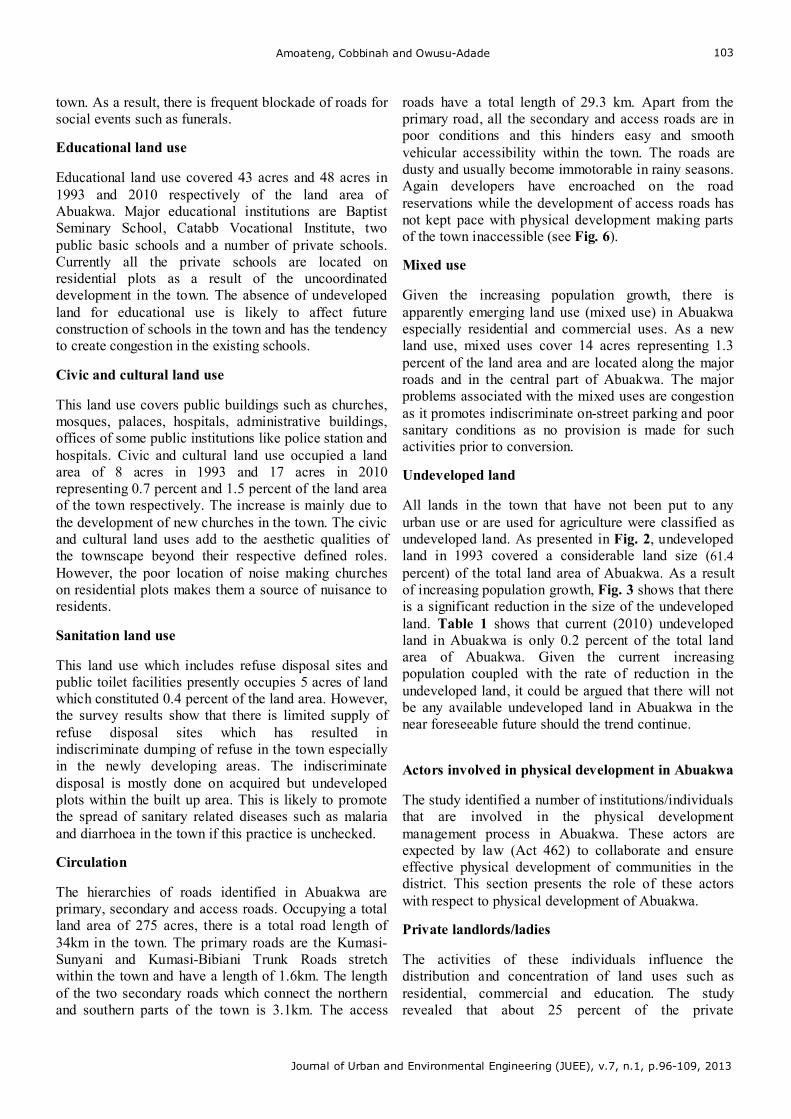
Amoateng, Cobbinah and Owusu-Adade
Journal of Urban and Environmental Engineering (JUEE), v.7, n.1, p.96-109, 2013
103
town. As a result, there is frequent blockade of roads for social events such as funerals. Educational land use Educational land use covered 43 acres and 48 acres in 1993 and 2010 respectively of the land area of Abuakwa. Major educational institutions are Baptist Seminary School, Catabb Vocational Institute, two public basic schools and a number of private schools. Currently all the private schools are located on residential plots as a result of the uncoordinated development in the town. The absence of undeveloped land for educational use is likely to affect future construction of schools in the town and has the tendency to create congestion in the existing schools. Civic and cultural land use This land use covers public buildings such as churches, mosques, palaces, hospitals, administrative buildings, offices of some public institutions like police station and hospitals. Civic and cultural land use occupied a land area of 8 acres in 1993 and 17 acres in 2010 representing 0.7 percent and 1.5 percent of the land area of the town respectively. The increase is mainly due to the development of new churches in the town. The civic and cultural land uses add to the aesthetic qualities of the townscape beyond their respective defined roles. However, the poor location of noise making churches on residential plots makes them a source of nuisance to residents. Sanitation land use This land use which includes refuse disposal sites and public toilet facilities presently occupies 5 acres of land which constituted 0.4 percent of the land area. However, the survey results show that there is limited supply of refuse disposal sites which has resulted in indiscriminate dumping of refuse in the town especially in the newly developing areas. The indiscriminate disposal is mostly done on acquired but undeveloped plots within the built up area. This is likely to promote the spread of sanitary related diseases such as malaria and diarrhoea in the town if this practice is unchecked. Circulation The hierarchies of roads identified in Abuakwa are primary, secondary and access roads. Occupying a total land area of 275 acres, there is a total road length of 34km in the town. The primary roads are the Kumasi-Sunyani and Kumasi-Bibiani Trunk Roads stretch within the town and have a length of 1.6km. The length of the two secondary roads which connect the northern and southern parts of the town is 3.1km. The access
roads have a total length of 29.3 km. Apart from the primary road, all the secondary and access roads are in poor conditions and this hinders easy and smooth vehicular accessibility within the town. The roads are dusty and usually become immotorable in rainy seasons. Again developers have encroached on the road reservations while the development of access roads has not kept pace with physical development making parts of the town inaccessible (see Fig. 6). Mixed use Given the increasing population growth, there is apparently emerging land use (mixed use) in Abuakwa especially residential and commercial uses. As a new land use, mixed uses cover 14 acres representing 1.3 percent of the land area and are located along the major roads and in the central part of Abuakwa. The major problems associated with the mixed uses are congestion as it promotes indiscriminate on-street parking and poor sanitary conditions as no provision is made for such activities prior to conversion. Undeveloped land All lands in the town that have not been put to any urban use or are used for agriculture were classified as undeveloped land. As presented in Fig. 2, undeveloped land in 1993 covered a considerable land size (61.4 percent) of the total land area of Abuakwa. As a result of increasing population growth, Fig. 3 shows that there is a significant reduction in the size of the undeveloped land. Table 1 shows that current (2010) undeveloped land in Abuakwa is only 0.2 percent of the total land area of Abuakwa. Given the current increasing population coupled with the rate of reduction in the undeveloped land, it could be argued that there will not be any available undeveloped land in Abuakwa in the near foreseeable future should the trend continue. Actors involved in physical development in Abuakwa The study identified a number of institutions/individuals that are involved in the physical development management process in Abuakwa. These actors are expected by law (Act 462) to collaborate and ensure effective physical development of communities in the district. This section presents the role of these actors with respect to physical development of Abuakwa. Private landlords/ladies The activities of these individuals influence the distribution and concentration of land uses such as residential, commercial and education. The study revealed that about 25 percent of the private
Amoateng, Cobbinah and Owusu-Adade
Journal of Urban and Environmental Engineering (JUEE), v.7, n.1, p.96-109, 2013
104
landlords/ladies have acquired and encroached on land demarcated as unbuildable and environmentally sensitive areas such as marshy and water ways. Traditional leaders In the context of Ghana, traditional leaders are considered as custodians of land, and are responsible for leasing land to both prívate and public developers. However, they are limited by law to determine the use of land, which is the responsibility of the TCPD. The study results indicate that there are seven (7) traditional leaders in Abuakwa, with each controlling the leasing and allocation of the land under his jurisdiction to prospective developers. It was however noted that the activities of these traditional leaders are not coordinated. As a consequence, there have been several cases of double allocation and land litigation in Abuakwa. In constrast to their fundamental role as custodians of the land, they have also assumed the role of determining the use in which a paticular land is put to. This situation has resulted in the leasing of lands which are demarcated by the TCPD for public uses, such as open spaces, for residential development. Town and Country Planning Department (TCPD) The TCPD was established in 1945 by the Town and Country Planning Ordinance of 1945 (CAP 84). The TCPD is a service delivery department under the Ministry of Environment, Science and Technology at the national level and the Ministry of Local Government and Rural Development at the local level. It has the responsibility of planning and managing the growth and development of all settlements in the country. From the study it was realized that the TCPD in the AND regulates physical development in Abuakwa through the preparation of planning schemes, issuance of building/development permits and monitoring and site inspection. Unfortunately, the Department is under resourced in terms of personnel and logistics which have hindered planning effort as well as routine monitoring of physical development in Abuakwa. The Department also faces the challenge of poor coordination and cooperation from other institutions especially traditional leaders. Atwima Nwabiagya District Assembly (ANDA) The Local Government Act (Act 462) mandates all metropolitan, municipal and district assemblies in Ghana with the responsibility of ensuring socio-economic and physical development of all communities in the district. As such, the ANDA oversees and coordinates the preparation and implementation of planning schemes to guide the growth and development
of all the communities in the district including Abuakwa. However, the study results show that the ANDA is unable to provide the development control institutions with adequate logistics to enable them function effectively. As a result, there is high prevalence of haphazard and unauthorized physical development in the most of the communities in the district including Abuakwa. Building Inspectorate Division (BID) This Division was established under the Metropolitan, Municipal and District Assemblies and is responsible for ensuring the enforcement of and compliance with building regulations. The Division in the AND is supposed to carry out this function by inspecting progress of development in Abuakwa and other communities in the district. However, the Division rarely functions as it is handicapped in the areas of logistics such as vehicles for inspection. The Division is also confronted with limited operational powers and lack of support and collaboration from other physical development management stakeholders. State Housing Company Limited (SHCL) The SHCL formerly Gold Coast Housing Corporation was established in 1955 as the main housing development agency of the Government of Ghana to ensure efficient housing development in the country. The company’s influence on the physical development of Abuakwa is manifested in its acquisition of land and construction of houses for the middle income group and workers of both the formal and informal sectors in the northern part of the town. The study analysis shows that this action of the company has contributed significantly to the rapid expansion of the town, although the development was undertaken in an orderly manner.
From the above discussions, it is ostensibly clear that physical development in Abuakwa involves many actors, some which are categorized under different parent institutions with diverse interests. As a consequence, there is lack of coordination and cooperation among the actors which has contributed to haphazard development, conflicting land uses and break down of formal development control processes in Abuakwa. Housing development in Abuakwa Houses are the most important manifestation of physical development in Abuakwa. The acquisition of development and building permits is the main prerequisite for carrying out any physical development in Ghana especially in areas that have Approved Planning Schemes. This is done to regulate the type,
Amoateng, Cobbinah and Owusu-Adade
Journal of Urban and Environmental Engineering (JUEE), v.7, n.1, p.96-109, 2013
105
nature and characteristics of the housing or physical development that are carried out on any piece of land. The survey revealed that 58.0 percent of house owners acquired development and building permits from planning authorities while 42.0 percent did not acquire any permits before developing their lands. This indicates that almost half of housing development in Abuakwa had not been authorized by the planning authorities. The reasons cited for the refusal to acquire permits were the high cost and bureaucratic processes or delays involved in the acquisition of permits.
Additionally, the traditional leaders have set a certain timeframe for the developers to start construction. This timeframe, which differs from one traditional leader to another, when elapsed, permits the traditional leaders to demand extra money or lease the land to another developer. As a result, prospective developers resort to development without planning authorities’ approval. This situation further highlights the haphazard and unregulated nature of physical development in Abuakwa.
The study revealed that majority of the houses (67 percent) fall into the single family detached houses category. Other housing types were compound and semi-detached which constituted 26 percent and 7 percent of the total housing stock respectively. The dominance of the detached houses is attributed to the settlement’s transformation from rural to urban status which has led to a steady shift from the traditional compound housing to modern single family housing system. This current housing preference has contributed to the rapid expansion of the town as the single family detached houses accommodate few people per square kilometer and consumes more land leading to the lateral expansion of the town. Characteristics of physical development in Abuakwa Leap frog development It was realized from the study that physical development in the town has occurred in a spatially fragmented pattern, due to speculative buying or acquisition of land. This has resulted in the presence of patched of undeveloped land (brown fields) located within the built up areas. The survey found that such green field sites occupy about 55 acres of the total residential land area of the town. According to the TCPD at ANDA, the leap frog development in the town is fuelled by double allocation of lands by land owners (traditional leaders) which has led to land litigation as well as incremental housing development, which is a common phenomenon in Ghana. These undeveloped patches of land serve as den for criminals and sites for indiscriminate disposal of refuse leading to wasteful and unsustainable use of land.
Land use (in) compatibility Analysis of land use location and relationship showed that there is high level of land use compatibility in Abuakwa because of the dominance of residential development (see Fig. 3). However, major cases of land use incompatibility identified included a noisy making and obnoxious odour emitting industrial activities such as metal products, processing firms and a poorly managed abattoir all located in the midst of the residential areas. These activities need to be grouped on a clearly defined location to internalize the problems associated with them. Land use change As presented in Table 1, it was observed from the study that Abuakwa has been characterized by substantial land use conversion mainly from undeveloped to residential as well as the introduction of mixed uses (e.g. location of residential and commercial uses in a single building). While the residential land use has extended into the undeveloped land and facilitated the lateral growth of Abuakwa, the mixed uses are concentrated along the major roads and in the Central Business District of the town. The development of mixed uses is fuelled by the desire of the house owners to earn high rent; as data gathered show that a single residential room earns a monthly average rent of GH¢10.00 while a store room goes for GH¢30.00. Despite the emergence of mixed uses, none of the house owners acquired permit before effecting the changes in the use of their buildings. This indicates the extent of non-compliance to planning regulations which is a threat to orderly and sustainable physical development. The negative consequences of such unauthorized conversion include traffic congestion and poor sanitary conditions. This land use change is likely to continue as the town becomes more urbanized and as such efforts should be made by the planning authorities to order its occurrence in the future. Physical development or land use zones As a typical peri-urban area, Abuakwa depicts three distinctive spatial zones. The zones include the core or indigenous, newly developed area or urban shadow and estate housing areas as illustrated spatially in Fig. 5. The core or indigenous area is where physical development started and is dominated by multi-family compound houses with most of them (85%) having existed for more than forty years. The zone is characterized by mixed land uses due to the conversion of buildings to commercial and residential uses by the house owners. Figure 5 shows the land use zones in Abuakwa.
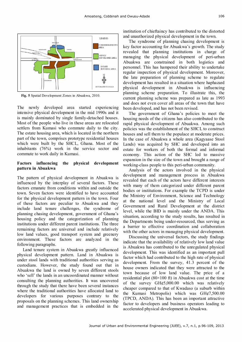
Amoateng, Cobbinah and Owusu-Adade
Journal of Urban and Environmental Engineering (JUEE), v.7, n.1, p.96-109, 2013
106
The newly developed area started experiencing intensive physical development in the mid 1990s and it is mainly dominated by single family-detached houses. Most of the people who live in these areas are relocated settlers from Kumasi who commute daily to the city. The estate housing area, which is located in the northern part of the town, comprises prototype residential houses which were built by the SHCL, Ghana. Most of the inhabitants (76%) work in the service sector and commute to work daily in Kumasi. Factors influencing the physical development pattern in Abuakwa The pattern of physical development in Abuakwa is influenced by the interplay of several factors. These factors emanate from conditions within and outside the town. Seven factors were identified to have accounted for the physical development pattern in the town. Four of these factors are peculiar to Abuakwa and they include land tenure challenges, the syndrome of planning chasing development, government of Ghana’s housing policy and the categorization of planning institutions under different parent institutions. The three remaining factors are universal and include relatively low land values, good transport system and greenery environment. These factors are analyzed in the following paragraphs.
Land tenure system in Abuakwa greatly influenced physical development pattern. Land in Abuakwa is under stool lands with traditional authorities serving as custodians. However, the study found out that in Abuakwa the land is owned by seven different stools who ‘sell’ the lands in an uncoordinated manner without consulting the planning authorities. It was uncovered through the study that there have been several instances where the traditional authorities have allocated land to developers for various purposes contrary to the proposals on the planning schemes. This land ownership and management practices that is embedded in the
institution of chieftaincy has contributed to the distorted and unauthorized physical development in the town.
The syndrome of planning chasing development is key factor accounting for Abuakwa’s growth. The study revealed that planning institutions in charge of managing the physical development of peri-urban Abuakwa are constrained in both logistics and personnel. This has hampered their ability to undertake regular inspection of physical development. Moreover, the late preparation of planning scheme to regulate development has resulted in a situation where haphazard physical development in Abuakwa is influencing planning scheme preparation. To illustrate this, the current planning scheme was prepared as late as 1993 and does not even cover all areas of the town that have been developed, and has not been revised.
The government of Ghana’s policies to meet the housing needs of the citizens has also contributed to the rapid physical development of Abuakwa. Among such policies was the establishment of the SHCL to construct houses and sell them to the populace at moderate prices. In the case of Abuakwa a whole area (Kagyaase Stool Lands) was acquired by SHC and developed into an estate for workers of both the formal and informal economy. This action of the SHC led to massive expansion in the size of the town and brought a range of working-class people to this peri-urban community.
Analysis of the actors involved in the physical development and management process in Abuakwa revealed that each of the actors have different interests with many of them categorized under different parent bodies or institutions. For example the TCPD is under the Ministry of Environment, Science and Technology at the national level and the Ministry of Local Government and Rural Development at the district level, while the BID is mainly under the ANDA. This situation, according to the study results, has resulted in the Departments being under-resourced, thus serving as a barrier to effective coordination and collaboration with the other actors in managing physical development.
Discussing the universal factors, the study findings indicate that the availability of relatively low land value is Abuakwa has contributed to the unregulated physical development. This was identified as an important pull factor which had contributed to the high rate of physical development. From the survey, 41.3 percent of the house owners indicated that they were attracted to the town because of low land value. The price of a residential plot (80×100 ft) in Abuakwa cost at the time of the survey GH¢5,000.00 which was relatively cheaper compared to that of Kwadaso (a suburb within the Kumasi Metropolis) which was GH¢7,500.00 (TPCD, ANDA). This has been an important attractive factor to developers and business operators leading to accelerated physical development in Abuakwa.
Fig. 5 Spatial Development Zones in Abuakwa, 2010.
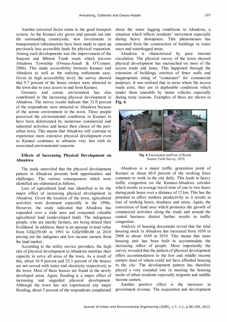
Amoateng, Cobbinah and Owusu-Adade
Journal of Urban and Environmental Engineering (JUEE), v.7, n.1, p.96-109, 2013
107
Another universal factor relate to the good transport system. As the Kumasi city grows and spreads out into the surrounding countryside, new investments in transportation infrastructure have been made to open up previously less accessible lands for physical expansion. Among such developments was the improvement of the Sunyani and Bibiani Trunk roads which traverse Abuakwa Township (Owusu-Ansah & O’Connor, 2006). This made accessibility between Kumasi and Abuakwa as well as the outlying settlements easy. Given its high accessibility level, the survey showed that 9.7 percent of the house owners were attracted to the town due to easy access to and from Kumasi.
Greenery and serene environment has also contributed to the increasing physical development in Abuakwa. The survey results indicate that 32.0 percent of the respondents were attracted to Abuakwa because of the serene environment in the town. These people perceived the environmental conditions in Kumasi to have been deteriorated by numerous commercial and industrial activities and hence their choice of the peri-urban town. This means that Abuakwa will continue to experience more extensive physical development even as Kumasi continues to urbanize very fast with its associated environmental concerns.
Effects of Increasing Physical Development on
Abuakwa The study unraveled that the physical development
pattern in Abuakwa presents both opportunities and challenges. The various consequences which were identified are elaborated as follows.
Loss of agricultural land was identified to be the major effect of increasing physical development in Abuakwa. Given the location of the town, agricultural activities were dominant especially in the 1990s. However, the study indicated that Abuakwa has expanded over a wide area and consumed valuable agricultural land (undeveloped land). The indigenous people, who are mainly farmers, are being denied their livelihood. In addition, there is an upsurge in land value from GH¢250.00 in 1993 to GH¢5000.00 in 2010 pricing out the indigenes and low income earners from the land market.
According to the utility service providers, the high rate of physical development in Abuakwa outstrips their capacity to serve all areas of the town. As a result of this, about 36.9 percent and 25.3 percent of the houses are not served with water and electricity respectively in the town. Most of these houses are found in the newly developed areas. Again, flooding is a major effect of increasing and unguided physical development. Although the town has not experienced any major flooding, about 3 percent of the respondents complained
about the water lagging conditions in Abuakwa, a situation which affects residents’ movement especially during heavy downpours. This phenomenon has emanated from the construction of buildings in water ways and waterlogged areas.
Abuakwa is characterized by poor internal circulation. The physical survey of the town showed physical development has encroached on most of the access roads and lanes. This happened through the extension of buildings, erection of fence walls and inappropriate siting of “containers” for commercial purposes. It was realized that in areas where the access roads exist, they are in deplorable conditions which render them unusable by motor vehicles especially during rainy seasons. Examples of these are shown in Fig. 6.
Fig. 6 Encroached and Poor of Roads. Source: Field Survey, 2010
Abuakwa is a major traffic generation point of
Kumasi as about 60.0 percent of the working force commute to work in the city daily. This leads to heavy traffic congestion on the Kumasi-Abuakwa corridor which results in average travel time of one to two hours during peak hours over a distance of 12 km. This has the potential to affect workers productivity as it results in loss of working hours, tiredness and stress. Again, the conversion of land uses which promotes the growth of commercial activities along the roads and around the central business district further results in traffic congestion.
Analysis of housing documents reveal that the total housing stock in Abuakwa has increased from 1030 in 2000 to about 1630 in 2010. This means that more housing unit has been built to accommodate the increasing influx of people. More importantly the survey revealed that the pattern of physical development offers accommodation to the low and middle income earners most of whom could not have afforded housing in the city. The development pattern has therefore played a very essential role in meeting the housing needs of urban residents especially migrants and middle income earners.
Another positive effect is the increases in government revenue. The acquisition and development
Amoateng, Cobbinah and Owusu-Adade
Journal of Urban and Environmental Engineering (JUEE), v.7, n.1, p.96-109, 2013
108
of land for housing, industries and businesses has led to increase in ground rent, taxes and property rates to the ANDA. In Abuakwa, annual ground rents and property rates are around GH¢8 and GH¢20 respectively per house. This shows the contribution of physical development in peri-urban areas to government revenue.
Managing physical development in peri-urban Abuakwa: the way forward
Central to this study is the understanding and assessment of the increasing physical development in peri-urban areas. The above discussions have portrayed the nature, extent and intensity of physical development in Abuakwa. The following paragraphs suggest ways of managing the increasing physical development in peri-urban Abuakwa.
To begin with, haphazard physical development in Abuakwa needs to be checked through strong institutions. The practice of planning chasing development should be checked. In relation to this, the study recommends that the state institutions concerned with physical development and land management should collaborate with the traditional authorities in the allocation of land to developers. The state institutions should be well resourced to help them examine building permits, undertake routine patrols and engage with community members in their efforts to curtail the unauthorized developments which have characterized peri-urban areas.
There is the need for the TCPD to embark on continuous and intensive public education on the processes involved in carrying out physical development. Stakeholders especially the traditional authorities and developers should be sensitized on their roles in ensuring orderly physical development. Popular participation in plan preparation should be encouraged to enable the residents understand the dynamics of physical development.
There is the need to establish CLS to co-ordinate the acquisition and allocation of land. This will ensure that decision regarding the allocation of land is well controlled and monitored instead of leaving it at the discretion of traditional leaders. This has the potential to ensure that developers receive the needed documentation covering their lands before development. The establishment of the CLS will help realize the objectives of the Land Administration Project (LAP) which is being implemented on pilot basis in some parts of Ghana.
It is recommended that physical development efforts in peri-urban areas should embrace the tenets of settlement growth management. The growth management approach should anticipate the rapid development which characterizes peri-urban areas and
make provision for directing and managing it. The major elements of the growth management should include the following;
1. Development should be restricted within
defined serviceable boundary. In this regard provision of services should be limited within the boundary. This will promote land use intensification and reduce the cost of providing utility services by forestalling rapid lateral expansion;
2. Phasing of development so as to manage development in specified areas within a time frame. This will enable development authorities to well monitor the growth of these areas and ensure orderly and functional settlement development in the long run;
3. Development and building permits should not be issued for areas where services have not been provided. This will ensure that every house has access to basic services. Physical development and service provision should proceed concurrently;
4. The preparation of physical development plans for peri-urban areas should be done in the framework of regional planning. Planning of peri-urban areas should be integrated into a city-wide system. This has the tendency to cater for both the internal and external factors which interplay to shape the pattern of physical development in peri-urban areas; and
The preparation of planning schemes to guide
development of peri-urban areas should be premised on land capability or classification studies. The potential of every piece of land need to be assessed and utilized for such purpose. Agricultural land must be reserved for such purpose irrespective of the rate of demand for other urban land uses. This will help preserve the economic life of the people especially the indigenes. However where farming or agriculture cannot be maintained, alternative livelihood need to be provided for the indigenes or the people.
CONCLUSION Although this paper has confirmed the general assertion that peri-urban areas experience rapid physical development (O’Sullivan, 2000; Hewitt, 1989; Buxton, 2007), and that they are characterized by high rates physical growth rate with the potential of tripling in physical size in every two decades, it has also identified certain physical development factors which are locally based.
The paper points out that the pattern of physical development is influenced by a number of local factors and they include: land tenure system and its associated traditional land management challenges; the categorization of planning institutions under different parent institutions, the syndrome of planning chasing development and the government of Ghana’s housing policy. The study has revealed that the resultant
Amoateng, Cobbinah and Owusu-Adade
Journal of Urban and Environmental Engineering (JUEE), v.7, n.1, p.96-109, 2013
109
physical development which emerges through the interplay of these factors has many negative effects on the residents of peri-urban areas. These adverse consequences include loss of agricultural land, lack of access to utility services, incidences of flooding, unregulated conversion of land uses, poor internal circulation and traffic congestion.
The study therefore recommends the strengthening of planning institutions, effective coordination and collaboration between planning institutions and the application of the tenets of settlement growth management. The growth management approach has the potential of foreseeing the rapid development which characterizes peri-urban areas as result of fast urbanization and make provision for it. Consequently, this has the tendency of reversing the trend of ‘planning chasing development’ into ‘planning directing and managing development’ in peri-urban Abuakwa. Concomitantly, the adoption and implementation of the settlement growth management approach will promote orderly physical development in the urban fringes and create liveable, functional and sustainable peri-urban areas. REFERENCES Adesina A, (2007) Socio-Spatial Transformations and the Urban
Fringe Landscape in Developing Countries, Nigeria: Ibadan University Press.
Atwima Nwabiagya District Assembly (2006) Medium Term Development Plan 2006-2009, Nkawie: ANDA
Balchin, P.N., Isaac, D. & Chen, J. J. (2000) Urban Ecoomics, A Global Perspective, United States: Palgrave Macmillan.
Buxton, M. (2007) Change in Peri-urban Australia: Implications for Land Use Policies, Australia: Department of Environment and Heritage Publishing Unit.
Cobbinah, P. B. & Amoako, C. (2012) Urban Sprawl and the Loss of Peri-Urban Land in Kumasi, Ghana. International Journal of Social and Human Sciences, 6, 388-397
Drabkin, D. H. (1977) Land Policy and Urban Growth, London: Pergamon Press.
Drescher. A. W. & Iaquinta D. L. (2000) Defining Peri-urban: Understanding Rural- Urban Linkages and their Connection to Institutional Contexts, Paper Presented at the Tenth World Congress, IRSA, Rio, August.
du Plessis, C. & Landman K. (2002) Sustainability Analysis of Human Settlements in South Africa, A report prepared by CSIR Building and Construction Technology Programme for Sustainable Human Settlement, Pretoria. Retrieved fromhttp://researchspace.csir.co.za/dspace/bitstream/10204/3522/1/u%20Plessis_2002.pdf on 12/07/2012
Ghana Statistical Service (2012) 2010 Population and Housing Census, Summary of Final Results, Accra: Ghana Statistical Service
Government of Swaziland (1997) The Draft Peri-Urban Growth Policy, 1997, Retrieved on 09/08/2010 from http://www.ecs.co.sz/periurban/pup_periurban_policy.htm
Hewitt, M. (1989) Defining "rural" Areas: Impact on Health Care Policy and Research. Health Program, Office of Technology Assessment, Congress of the United States, Washington, DC
Johnson, J.H. (1974) Suburban Growth, Geographical Process at the Edge of the Western City, Aberdeen: Aberdeen University Press.
Keeble, L. (1969) Principles of Town and Country Planning, London: The Estate Gazette Limited.
Mather, A.S. (1989) Land Use, New York: Wiley and Sons Inc. Miller, R. L. & Brewer, J. D. (2003) A – Z of Social Research.
London: SAGE Publication Ltd Mohd Noor, K. B. (2008) Case study: A strategic research
methodology. American Journal of Applied Sciences, 5(11), 1602-1604.
National Development Planning Commission (2004) Atwima District Human Development Report, Accra, Ghana: NDPC.
O’Sullivan, A, (2000) Urban Economics, United States: The McGraw Hill Companies Inc.
Organisation for Economic Co-operation and Development (OECD), (2007) The Growing Peri-Urban Phenomenon, Report of One Week Conference held in France.
Owusu-Ansah, J. & O.Connor, K. (2006) Transportation and Physical Development around Kumasi in Ghana, Discussion Paper Submitted to World Academy of Science, Engineering and Technology.
Sarantakos, S. (1998). Social Research, London: McMillan Press Ltd.
Timms, P. (2006) Peri-Urban Development, Conference Presentation at the European Aid Co-operation Centre in China.
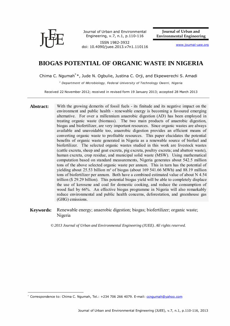
Ngumah, Ogbulie, Orji and Amadi
Journal of Urban and Environmental Engineering (JUEE), v.7, n.1, p.110-116, 2013
110
Journal of Urban and Environmental Engineering, v.7, n.1, p.110-116
Journal of Urban and Environmental Engineering
UEEJ ISSN 1982-3932
doi: 10.4090/juee.2013.v7n1.110116 www.journal-uee.org
BIOGAS POTENTIAL OF ORGANIC WASTE IN NIGERIA
Chima C. Ngumah*, Jude N. Ogbulie, Justina C. Orji, and Ekpewerechi S. Amadi 1 Department of Microbiology, Federal University of Technology Owerri, Nigeria
Received 22 November 2012; received in revised form 19 January 2013; accepted 28 March 2013
Abstract: With the growing demerits of fossil fuels - its finitude and its negative impact on the
environment and public health - renewable energy is becoming a favoured emerging alternative. For over a millennium anaerobic digestion (AD) has been employed in treating organic waste (biomass). The two main products of anaerobic digestion, biogas and biofertilizer, are very important resources. Since organic wastes are always available and unavoidable too, anaerobic digestion provides an efficient means of converting organic waste to profitable resources. This paper elucidates the potential benefits of organic waste generated in Nigeria as a renewable source of biofuel and biofertilizer. The selected organic wastes studied in this work are livestock wastes (cattle excreta, sheep and goat excreta, pig excreta, poultry excreta; and abattoir waste), human excreta, crop residue, and municipal solid waste (MSW). Using mathematical computation based on standard measurements, Nigeria generates about 542.5 million tons of the above selected organic waste per annum. This in turn has the potential of yielding about 25.53 billion m³ of biogas (about 169 541.66 MWh) and 88.19 million tons of biofertilizer per annum. Both have a combined estimated value of about N 4.54 trillion ($ 29.29 billion). This potential biogas yield will be able to completely displace the use of kerosene and coal for domestic cooking, and reduce the consumption of wood fuel by 66%. An effective biogas programme in Nigeria will also remarkably reduce environmental and public health concerns, deforestation, and greenhouse gas (GHG) emissions.
Keywords:
Renewable energy; anaerobic digestion; biogas; biofertilizer; organic waste; Nigeria
© 2013 Journal of Urban and Environmental Engineering (JUEE). All rights reserved.
Correspondence to: Chima C. Ngumah, Tel.: +234 706 266 4079. E-mail: [email protected]
Ngumah, Ogbulie, Orji and Amadi
Journal of Urban and Environmental Engineering (JUEE), v.7, n.1, p.110-116, 2013
111
INTRODUCTION
Biogas technology, also known as anaerobic digestion (AD) technology, is the use of biological processes in the absence of oxygen for the breakdown of organic matter and the stabilization of these material, by conversion to biogas and nearly stable residue (digestate) (Marchaim, 1992). Biogas is a mixture of methane (4575%) and carbon dioxide (2555%); the actual proportion depending on the feedstock (substrate) used and processes employed. For biogas to be flammable the methane content must be ≥ 40%. Apart from methane and carbon dioxide, biogas may also contain small amounts (≤ 3%) of impurities, such as hydrogen sulphide, ammonia, carbon monoxide, and other gases (Monnet, 2003).
Historical evidence indicates that AD is one of the oldest technologies. Even around 3000 BC the Sumerians practiced anaerobic cleansing of waste (Deublein & Steinhauser, 2008). However, the industrialization of anaerobic digestion began in 1859 with first AD plant sited in Bombay (India). In 1897, an anaerobic digester at Matunga Leper Asylum in Bombay used human waste to generate biogas (Khanal, 2008). According to Deublein & Steinhauser (2008), other countries that pioneered the evolution of biogas technology were:
France, in 1987 the streets lamps of Exeter started running on biogas produced from wastewater.
China, rural biogas system developed in 1920, while the national programme started in 1958.
Germany, agricultural products were used to produce biogas in 1945.
Today, China is credited as having the largest
biogas programme in the world with over 20 million biogas plants installed (Tatlidil et al., 2009). According to Deublein & Steinhauser (2008), biogas technology was introduced in Africa between 1930 and 1940 when
Ducellier and Isman started building simple biogas machines in Algeria to supply farmhouses with energy. Despite this early start in Africa the development of large scale biogas technology is still in its embryonic stage in this region, though with a lot of potentials. In Nigeria, the status of biogas technology remains abysmal. The earliest record of biogas technology in Nigeria was in the 80s when a simple biogas plant that could produce 425 litres of biogas per day was built at Usman Danfodiyo University, Sokoto (Dangogo & Fernado, 1986).
About 21 pilot demonstration plants with a capacity range of between 10m320m3 have been sited in different parts of the country.
The two main products of biogas technology are biogas (fuel) and biofertilizer (fertilizer) and the
benefits derived in employing AD in treating organic wastes are: Benefits for the energy sector:-
Source of renewable (green) energy, which leads to a lesser dependency on the finite fossil fuels.
The use of the digestate decreases the use of fossil fuels in the manufacturing of synthetic fertilizer.
It is carbon dioxide neutral. Benefits for agriculture:
Transformation of organic waste to very high quality fertilizer.
Improved utilization of nitrogen (by plants) from animal manure.
Balanced phosphorus/potassium ratio in digestate.
Homogenous and light fluid slurry. AD virtually destroy all weed seeds, thus
reducing the need for herbicides and other weed control measures.
Provides closed nutrient cycle. Treated effluent from AD is a good animal feed
when processed with molasses and grains. Benefits for the environment:-
Reduces emission of greenhouse gases (GHG). Reduces nitrogen leaching into ground and
surface waters. Improves hygiene through the reduction of
pathogens, worm eggs, and flies. Reduces odour by 80%. Controlled recycling/reduction of waste. Reduces deforestation by providing renewable
alternative to woodfuel and charcoal. Biogas burns “cleaner” than woodfuel,
kerosene, and undigested biowaste. It creates an integrated waste management
system which reduces the likelihood of soil and water pollution compared to the disposal of untreated biowastes.
Benefits to the economy:
Provides cheaper energy and fertilizer. Provides additional income to farmers. Creates job opportunities. Decentralizes energy generation and
environmental protection.
Mountainous heaps of open wastes dumps have continued to characterize urban centres in Nigeria. Different waste management institutions saddled with the responsibility of waste management have
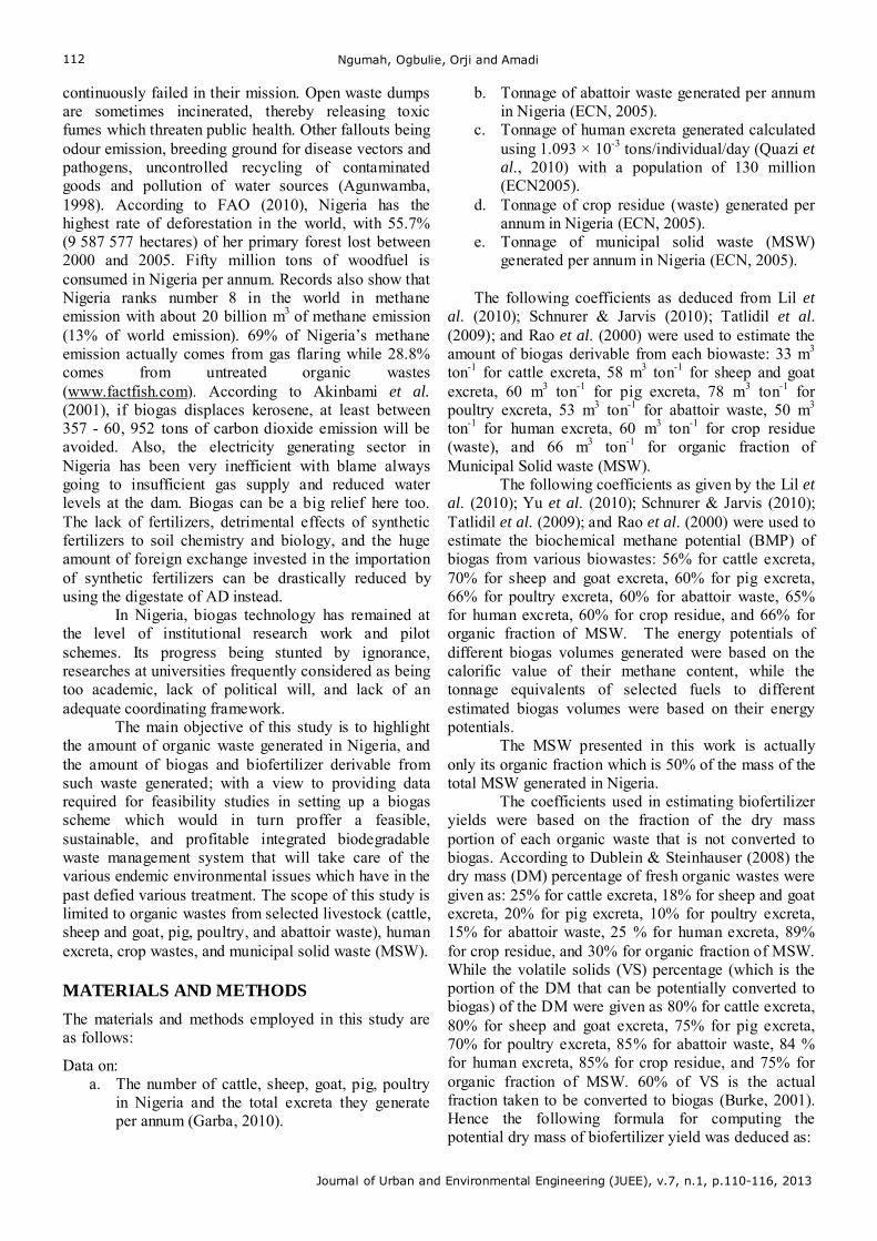
Ngumah, Ogbulie, Orji and Amadi
Journal of Urban and Environmental Engineering (JUEE), v.7, n.1, p.110-116, 2013
112
continuously failed in their mission. Open waste dumps are sometimes incinerated, thereby releasing toxic fumes which threaten public health. Other fallouts being odour emission, breeding ground for disease vectors and pathogens, uncontrolled recycling of contaminated goods and pollution of water sources (Agunwamba, 1998). According to FAO (2010), Nigeria has the highest rate of deforestation in the world, with 55.7% (9 587 577 hectares) of her primary forest lost between 2000 and 2005. Fifty million tons of woodfuel is consumed in Nigeria per annum. Records also show that Nigeria ranks number 8 in the world in methane emission with about 20 billion m3 of methane emission (13% of world emission). 69% of Nigeria’s methane emission actually comes from gas flaring while 28.8% comes from untreated organic wastes (www.factfish.com). According to Akinbami et al. (2001), if biogas displaces kerosene, at least between 357 - 60, 952 tons of carbon dioxide emission will be avoided. Also, the electricity generating sector in Nigeria has been very inefficient with blame always going to insufficient gas supply and reduced water levels at the dam. Biogas can be a big relief here too. The lack of fertilizers, detrimental effects of synthetic fertilizers to soil chemistry and biology, and the huge amount of foreign exchange invested in the importation of synthetic fertilizers can be drastically reduced by using the digestate of AD instead.
In Nigeria, biogas technology has remained at the level of institutional research work and pilot schemes. Its progress being stunted by ignorance, researches at universities frequently considered as being too academic, lack of political will, and lack of an adequate coordinating framework.
The main objective of this study is to highlight the amount of organic waste generated in Nigeria, and the amount of biogas and biofertilizer derivable from such waste generated; with a view to providing data required for feasibility studies in setting up a biogas scheme which would in turn proffer a feasible, sustainable, and profitable integrated biodegradable waste management system that will take care of the various endemic environmental issues which have in the past defied various treatment. The scope of this study is limited to organic wastes from selected livestock (cattle, sheep and goat, pig, poultry, and abattoir waste), human excreta, crop wastes, and municipal solid waste (MSW). MATERIALS AND METHODS
The materials and methods employed in this study are as follows:
Data on: a. The number of cattle, sheep, goat, pig, poultry
in Nigeria and the total excreta they generate per annum (Garba, 2010).
b. Tonnage of abattoir waste generated per annum in Nigeria (ECN, 2005).
c. Tonnage of human excreta generated calculated using 1.093 × 10⁻³ tons/individual/day (Quazi et al., 2010) with a population of 130 million (ECN2005).
d. Tonnage of crop residue (waste) generated per annum in Nigeria (ECN, 2005).
e. Tonnage of municipal solid waste (MSW) generated per annum in Nigeria (ECN, 2005).
The following coefficients as deduced from Lil et
al. (2010); Schnurer & Jarvis (2010); Tatlidil et al. (2009); and Rao et al. (2000) were used to estimate the amount of biogas derivable from each biowaste: 33 m3 ton-1 for cattle excreta, 58 m3 ton-1 for sheep and goat excreta, 60 m3 ton-1 for pig excreta, 78 m3 ton-1 for poultry excreta, 53 m3 ton-1 for abattoir waste, 50 m3 ton-1 for human excreta, 60 m3 ton-1 for crop residue (waste), and 66 m3 ton-1 for organic fraction of Municipal Solid waste (MSW).
The following coefficients as given by the Lil et al. (2010); Yu et al. (2010); Schnurer & Jarvis (2010); Tatlidil et al. (2009); and Rao et al. (2000) were used to estimate the biochemical methane potential (BMP) of biogas from various biowastes: 56% for cattle excreta, 70% for sheep and goat excreta, 60% for pig excreta, 66% for poultry excreta, 60% for abattoir waste, 65% for human excreta, 60% for crop residue, and 66% for organic fraction of MSW. The energy potentials of different biogas volumes generated were based on the calorific value of their methane content, while the tonnage equivalents of selected fuels to different estimated biogas volumes were based on their energy potentials.
The MSW presented in this work is actually only its organic fraction which is 50% of the mass of the total MSW generated in Nigeria.
The coefficients used in estimating biofertilizer yields were based on the fraction of the dry mass portion of each organic waste that is not converted to biogas. According to Dublein & Steinhauser (2008) the dry mass (DM) percentage of fresh organic wastes were given as: 25% for cattle excreta, 18% for sheep and goat excreta, 20% for pig excreta, 10% for poultry excreta, 15% for abattoir waste, 25 % for human excreta, 89% for crop residue, and 30% for organic fraction of MSW. While the volatile solids (VS) percentage (which is the portion of the DM that can be potentially converted to biogas) of the DM were given as 80% for cattle excreta, 80% for sheep and goat excreta, 75% for pig excreta, 70% for poultry excreta, 85% for abattoir waste, 84 % for human excreta, 85% for crop residue, and 75% for organic fraction of MSW. 60% of VS is the actual fraction taken to be converted to biogas (Burke, 2001). Hence the following formula for computing the potential dry mass of biofertilizer yield was deduced as:
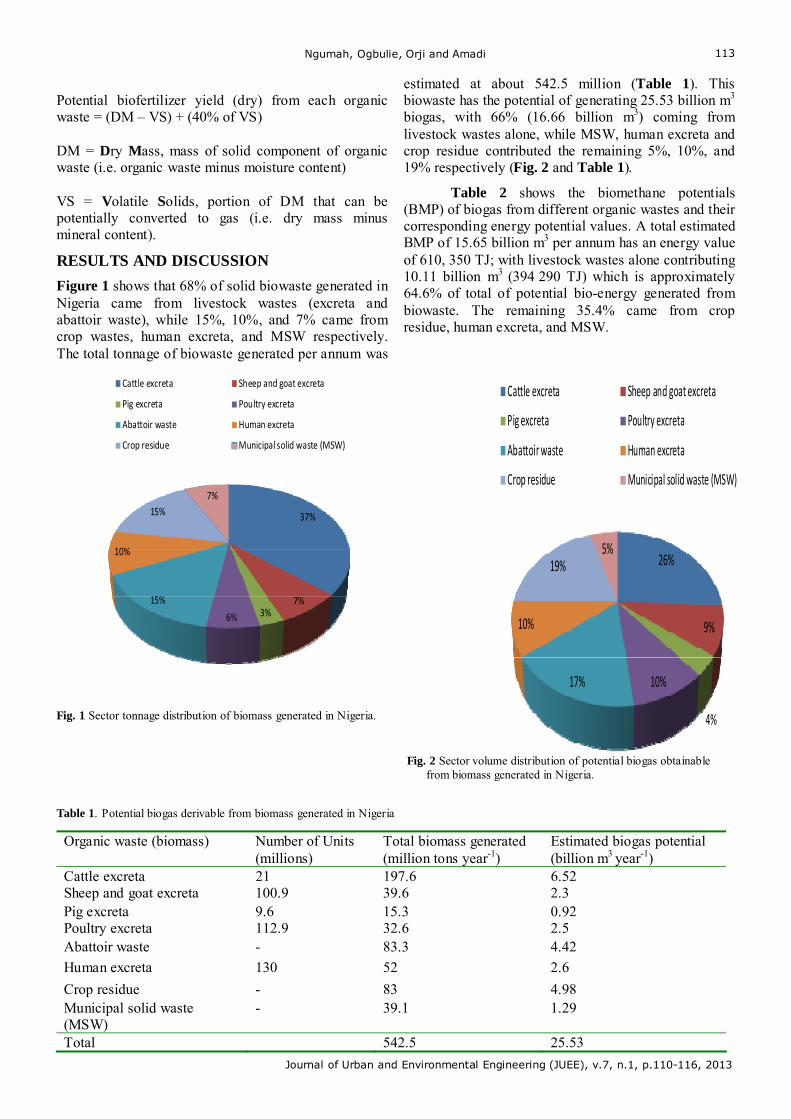
Ngumah, Ogbulie, Orji and Amadi
Journal of Urban and Environmental Engineering (JUEE), v.7, n.1, p.110-116, 2013
113
Potential biofertilizer yield (dry) from each organic waste = (DM – VS) + (40% of VS) DM = Dry Mass, mass of solid component of organic waste (i.e. organic waste minus moisture content) VS = Volatile Solids, portion of DM that can be potentially converted to gas (i.e. dry mass minus mineral content).
RESULTS AND DISCUSSION
Figure 1 shows that 68% of solid biowaste generated in Nigeria came from livestock wastes (excreta and abattoir waste), while 15%, 10%, and 7% came from crop wastes, human excreta, and MSW respectively. The total tonnage of biowaste generated per annum was
estimated at about 542.5 million (Table 1). This biowaste has the potential of generating 25.53 billion m3
biogas, with 66% (16.66 billion m3) coming from livestock wastes alone, while MSW, human excreta and crop residue contributed the remaining 5%, 10%, and 19% respectively (Fig. 2 and Table 1).
Table 2 shows the biomethane potentials (BMP) of biogas from different organic wastes and their corresponding energy potential values. A total estimated BMP of 15.65 billion m3 per annum has an energy value of 610, 350 TJ; with livestock wastes alone contributing 10.11 billion m3 (394 290 TJ) which is approximately 64.6% of total of potential bio-energy generated from biowaste. The remaining 35.4% came from crop residue, human excreta, and MSW.
37%
7%3%6%
15%
10%
15%
7%
Cattle excreta Sheep and goat excreta
Pig excreta Poultry excreta
Abattoir waste Human excreta
Crop residue Municipal solid waste (MSW)
Fig. 1 Sector tonnage distribution of biomass generated in Nigeria.
26%
9%
4%
10%17%
10%
19%5%
Cattle excreta Sheep and goat excreta
Pig excreta Poultry excreta
Abattoir waste Human excreta
Crop residue Municipal solid waste (MSW)
Fig. 2 Sector volume distribution of potential biogas obtainable from biomass generated in Nigeria.
Table 1. Potential biogas derivable from biomass generated in Nigeria
Organic waste (biomass) Number of Units (millions)
Total biomass generated (million tons year-1)
Estimated biogas potential (billion m3 year-1)
Cattle excreta 21 197.6 6.52 Sheep and goat excreta 100.9 39.6 2.3 Pig excreta 9.6 15.3 0.92 Poultry excreta 112.9 32.6 2.5 Abattoir waste - 83.3 4.42
Human excreta 130 52 2.6
Crop residue - 83 4.98 Municipal solid waste (MSW)
- 39.1 1.29
Total 542.5 25.53
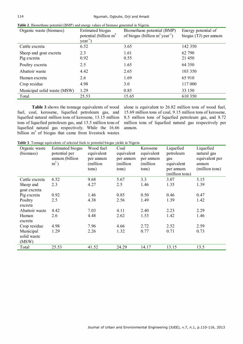
Ngumah, Ogbulie, Orji and Amadi
Journal of Urban and Environmental Engineering (JUEE), v.7, n.1, p.110-116, 2013
114
Table 2. Biomethane potential (BMP) and energy values of biomass generated in Nigeria.
Organic waste (biomass) Estimated biogas potential (billion m3
year-1)
Biomethane potential (BMP) of biogas (billion m3 year-1)
Energy potential of biogas (TJ) per annum
Cattle excreta 6.52 3.65 142 350
Sheep and goat excreta 2.3 1.61 62 790 Pig excreta 0.92 0.55 21 450
Poultry excreta 2.5 1.65 64 350
Abattoir waste 4.42 2.65 103 350
Human excreta 2.6 1.69 65 910 Crop residue 4.98 3.0 117 000
Municipal solid waste (MSW) 1.29 0.85 33 150 Total 25.53 15.65 610 350
Table 3 shows the tonnage equivalents of wood fuel, coal, kerosene, liquefied petroleum gas, and liquefied natural million tons of kerosene, 13.15 million tons of liquefied petroleum gas, and 13.5 million tons of liquefied natural gas respectively. While the 16.66 billion m3 of biogas that came from livestock wastes
alone is equivalent to 26.82 million tons of wood fuel, 15.69 million tons of coal, 9.15 million tons of kerosene, 8.5 million tons of liquefied petroleum gas, and 8.72 million tons of liquefied natural gas respectively per annum.
Table 3. Tonnage equivalents of selected fuels to potential biogas yields in Nigeria
Organic waste (biomass)
Estimated biogas potential per annum (billion m3 )
Wood fuel equivalent per annum (million tons)
Coal equivalent per annum (million tons)
Kerosene equivalent per annum (million tons)
Liquefied petroleum gas equivalent per annum (million tons)
Liquefied natural gas equivalent per annum (million tons)
Cattle excreta 6.52 9.68 5.67 3.3 3.07 3.15 Sheep and goat excreta
2.3 4.27 2.5 1.46 1.35 1.39
Pig excreta 0.92 1.46 0.85 0.50 0.46 0.47 Poultry excreta
2.5 4.38 2.56 1.49 1.39 1.42
Abattoir waste 4.42 7.03 4.11 2.40 2.23 2.29 Human excreta
2.6 4.48 2.62 1.53 1.42 1.46
Crop residue 4.98 7.96 4.66 2.72 2.52 2.59 Municipal solid waste (MSW)
1.29 2.26 1.32 0.77 0.71 0.73
Total 25.53 41.52 24.29 14.17 13.15 13.5
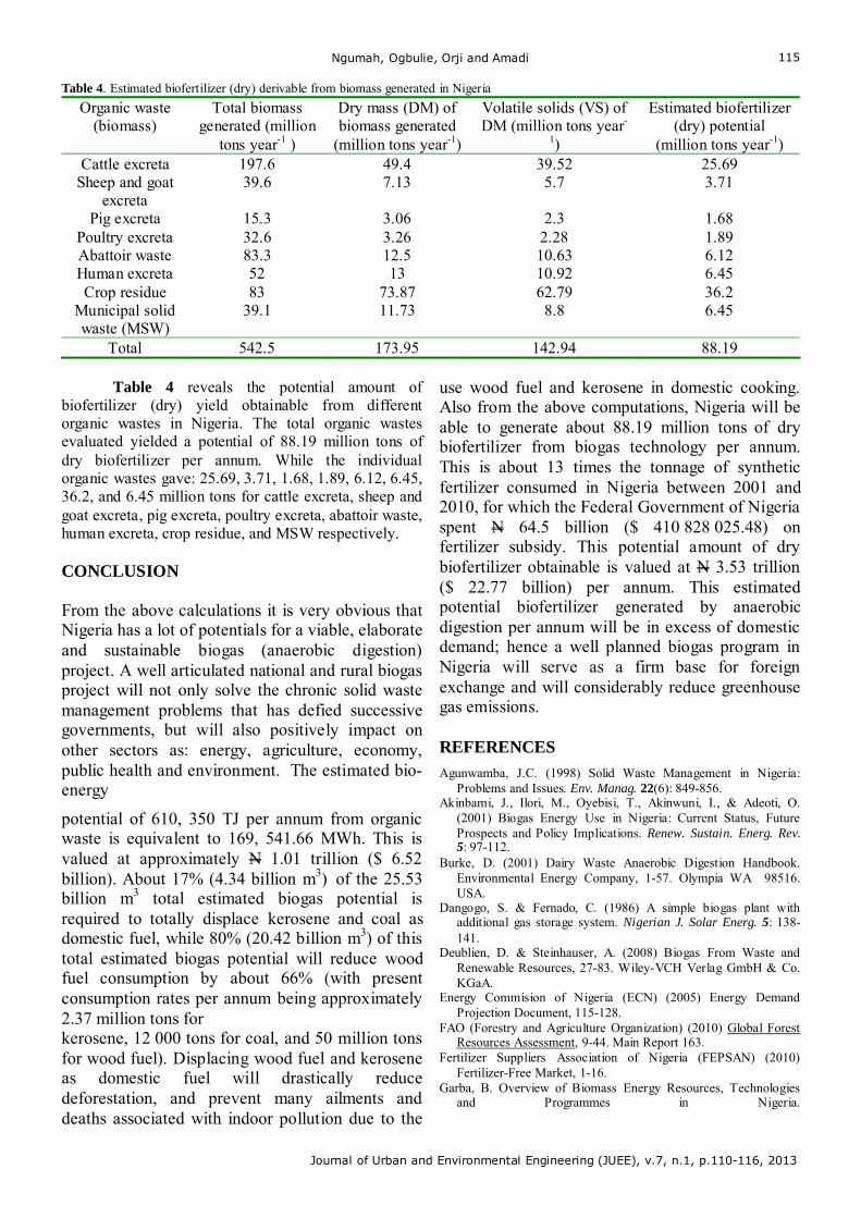
Ngumah, Ogbulie, Orji and Amadi
Journal of Urban and Environmental Engineering (JUEE), v.7, n.1, p.110-116, 2013
115
Table 4. Estimated biofertilizer (dry) derivable from biomass generated in Nigeria
Organic waste (biomass)
Total biomass generated (million
tons year-1 )
Dry mass (DM) of biomass generated
(million tons year-1)
Volatile solids (VS) of DM (million tons year-
1)
Estimated biofertilizer (dry) potential
(million tons year-1) Cattle excreta 197.6 49.4 39.52 25.69
Sheep and goat excreta
39.6 7.13 5.7 3.71
Pig excreta 15.3 3.06 2.3 1.68 Poultry excreta 32.6 3.26 2.28 1.89 Abattoir waste 83.3 12.5 10.63 6.12 Human excreta 52 13 10.92 6.45 Crop residue 83 73.87 62.79 36.2
Municipal solid waste (MSW)
39.1 11.73 8.8 6.45
Total 542.5 173.95 142.94 88.19
Table 4 reveals the potential amount of biofertilizer (dry) yield obtainable from different organic wastes in Nigeria. The total organic wastes evaluated yielded a potential of 88.19 million tons of dry biofertilizer per annum. While the individual organic wastes gave: 25.69, 3.71, 1.68, 1.89, 6.12, 6.45, 36.2, and 6.45 million tons for cattle excreta, sheep and goat excreta, pig excreta, poultry excreta, abattoir waste, human excreta, crop residue, and MSW respectively. CONCLUSION From the above calculations it is very obvious that Nigeria has a lot of potentials for a viable, elaborate and sustainable biogas (anaerobic digestion) project. A well articulated national and rural biogas project will not only solve the chronic solid waste management problems that has defied successive governments, but will also positively impact on other sectors as: energy, agriculture, economy, public health and environment. The estimated bio-energy
potential of 610, 350 TJ per annum from organic waste is equivalent to 169, 541.66 MWh. This is valued at approximately N 1.01 trillion ($ 6.52 billion). About 17% (4.34 billion m3) of the 25.53 billion m3 total estimated biogas potential is required to totally displace kerosene and coal as domestic fuel, while 80% (20.42 billion m3) of this total estimated biogas potential will reduce wood fuel consumption by about 66% (with present consumption rates per annum being approximately 2.37 million tons for kerosene, 12 000 tons for coal, and 50 million tons for wood fuel). Displacing wood fuel and kerosene as domestic fuel will drastically reduce deforestation, and prevent many ailments and deaths associated with indoor pollution due to the
use wood fuel and kerosene in domestic cooking. Also from the above computations, Nigeria will be able to generate about 88.19 million tons of dry biofertilizer from biogas technology per annum. This is about 13 times the tonnage of synthetic fertilizer consumed in Nigeria between 2001 and 2010, for which the Federal Government of Nigeria spent N 64.5 billion ($ 410 828 025.48) on fertilizer subsidy. This potential amount of dry biofertilizer obtainable is valued at N 3.53 trillion ($ 22.77 billion) per annum. This estimated potential biofertilizer generated by anaerobic digestion per annum will be in excess of domestic demand; hence a well planned biogas program in Nigeria will serve as a firm base for foreign exchange and will considerably reduce greenhouse gas emissions. REFERENCES
Agunwamba, J.C. (1998) Solid Waste Management in Nigeria: Problems and Issues. Env. Manag. 22(6): 849-856.
Akinbami, J., Ilori, M., Oyebisi, T., Akinwuni, I., & Adeoti, O. (2001) Biogas Energy Use in Nigeria: Current Status, Future Prospects and Policy Implications. Renew. Sustain. Energ. Rev. 5: 97-112.
Burke, D. (2001) Dairy Waste Anaerobic Digestion Handbook. Environmental Energy Company, 1-57. Olympia WA 98516. USA.
Dangogo, S. & Fernado, C. (1986) A simple biogas plant with additional gas storage system. Nigerian J. Solar Energ. 5: 138-141.
Deublien, D. & Steinhauser, A. (2008) Biogas From Waste and Renewable Resources, 27-83. Wiley-VCH Verlag GmbH & Co. KGaA.
Energy Commision of Nigeria (ECN) (2005) Energy Demand Projection Document, 115-128.
FAO (Forestry and Agriculture Organization) (2010) Global Forest Resources Assessment, 9-44. Main Report 163.
Fertilizer Suppliers Association of Nigeria (FEPSAN) (2010) Fertilizer-Free Market, 1-16.
Garba, B. Overview of Biomass Energy Resources, Technologies and Programmes in Nigeria.

Ngumah, Ogbulie, Orji and Amadi
Journal of Urban and Environmental Engineering (JUEE), v.7, n.1, p.110-116, 2013
116
(http://cgpl.iisc.ernet.in/site/Portals/0/Publications/Presentations/EGM/10_Nigeria-egm.pdf).
Khanal, S.K. (2008) Anaerobic Biotechnology for Bioenergy Production: Principles and Applications. Wiley-Blackwell. Ames.
Lil, S., Liangwei, D., Yong,Y., Xiaodong, P., Zhiyong, W. (2010) Biogas Production Potential and Characteristics of Manure of Sheep, Duck and Rabbit under Anaerobic Digestion. Chin. Soc. of Agric. Eng. 10(1), 22-34.
Marchaim, U. (1992) Biogas Processes for Sustainable Development, 1-99. FAO.
Matthew, R., Subedi, M., Smith, J., Yongabi, K., Avery, L., Starchan, N., & Semple, S. (2011) The Potential of Small-Scale Digesters to Alleviate Poverty and Improve Long Term Sustainability of Ecosystem Services in Sub-Saharan Africa. DFID NET-RC A06502.
Monnet, F. (2003) An Introduction to Anaerobic Digestion of Organic Wastes, 1-43. Final Report.
Quazi, A. & R. Islam. (2005) The Re-use of human Excreta in Bangladesh. (www.wateraid.org/documents/ch19).
Rao, S., Singh, S., Singh, A. & Sodha, M. (2000) Bioenergy Conversion Studies of the Organic Fraction of MSW: Assessment of Ultimate Bioenergy Production Potential of Municipal Garbage. Appl. Energ. 66(1): 11-18.
Sambo, A. (2009). Strategic Developments in Renewable Energy in Nigeria, 15-19. International Association of Energy Economy. Third Quarter.
Schnurer, A. & Jarvis, A. (2010) Microbiological Handbook for Biogas Plants, 1-74. Swedish Waste Management U2009:03. Swedish Gas Centre Report 207.
Tatlidil, F., Bayramoglu, Z. & Akturk, D. (2009) Animal Manure as One of the Main Biogas Production Resources: Case of Turkey. J. Anim. and Vet. Adv. 8(2): 2473-2476, 2009.
Yu, Z., M. Morrison, F. Schanbacher. (2010) Biomass to Biofuels: Strategies for Global Industries, 6-9. John Wiley & Sons Ltd. United Kingdom.
Affam and Adlan
Journal of Urban and Environmental Engineering (JUEE), v.7, n.1, p.117-125, 2013
117
Journal of Urban and Environmental Engineering, v.7, n.1, p.117-125
Journal of Urban and Environmental Engineering
UEEJ ISSN 1982-3932
doi: 10.4090/juee.2013.v7n1.117125 www.journal-uee.org
OPERATIONAL PERFORMANCE OF VERTICAL UPFLOW ROUGHING FILTER FOR PRE-TREATMENT OF LEACHATE
USING LIMESTONE FILTER MEDIA
Augustine Chioma Affam1 and Mohd. Nordin Adlan2
1, 2 School of Civil Engineering, Universiti Sains Malaysia, Engineering Campus, Nibong Tebal, Penang, Malaysia
1 Department of Civil Engineering, Universiti Teknologi PETRONAS, Badar Seri Iskandar, Tronoh, Perak, Malaysia
Received 25 April 2012; received in revised form 30 January 2013; accepted 09 February 2013
Abstract: This study was conducted to investigate the removal of COD, BOD, turbidity and
colour from leachate using vertical upflow filtration technique. Limestone media with a density of 2554 kg/m3 was crushed and graded in sizes of 48 mm, 812 mm and 1218 mm. Trial runs were done before the main experiment at an interval of 24 h analysis. Leachate was between pH 7.94 to 8.12 before experiments but increased to pH 8.42 after the filtration process. Maximum headloss at steady flow rate 20mL/min was 0.5 cm. The optimum treatment was achieved with 4–8 mm, 8–12 mm & 12–18 mm media size in combination and removal efficiency was 22 to 81%, 22 to 75%, 32 to 86%, and 36 to 62% for BOD, COD, turbidity and colour, respectively. Vertical upflow roughing filter can be used for pre-treatment of leachate before further treatment.
Keywords:
Limestone; vertical upflow roughing Filter; leachate; landfill.
© 2013 Journal of Urban and Environmental Engineering (JUEE). All rights reserved.
Correspondence to: Augustine C. Affam, Tel: +60103849701. E-mail: [email protected]
Affam and Adlan
Journal of Urban and Environmental Engineering (JUEE), v.7, n.1, p.117-125, 2013
118
INTRODUCTION
A leachate stream can be compared to a complex wastewater stream with varying characteristics not only because of the different kinds of waste present, but also varying according to the landfill age (Onay & Pohland, 1998). The leakage of leachate from landfill which contains high organic, inorganic, suspended solids, heavy metals and other pollutants can contaminate the ground water and surface water sources (Qasim & Chiang, 1994). The high level of chemical oxygen demand (COD), biochemical oxygen demand (BOD), turbidity, colour and other impurity components of landfill leachate make it very important to devise appropriate treatment methods.
Leachate used in this research was collected from Pulau Burung Landfill Site (PBLS) which is situated in Penang, Malaysia. PBLS has a semi-aerobic system and it is one of the only three sites of its kind found in Malaysia. PBSL has been developed semi-aerobically into a sanitary landfill Level II by establishing a controlled tipping technique in 1991. It was further upgraded to a sanitary landfill Level III employing controlled tipping with leachate recirculation in 2001. It has been found that the leachate from a semi-aerobic system has slightly lower organic contaminants compared with an anaerobic landfill in terms of BOD and COD (Aziz et al., 2001). This site receives 1500 tons of solid waste daily. Table 1 gives the composition of the leachate.
There are many different landfill leachate treatment options. These include complex and expensive methods from physico-chemical to biological processes for the treatment of high strength organics and inorganics. These could result in large costs on the long term. Alternative methods are continually sought to minimize expenses on leachate treatment (Tchobanoglous et al., 2003).
Roughing filtration can be considered as a major pre-treatment process for wastewater and surface water, since the process efficiently separates fine solid particles over prolonged periods without addition of Table 1. Composition of Leachate from Pulau Burung Landfill Site
Parameters Range of Values, mg/L
BOD5 481120 COD 15333600 Suspended Solid 1591220 pH value (no unit) 7.89.4 Zinc 0.11.8 Manganese 0.6–1.1 Iron 0.32–7.5 Copper 0.1–0.4 Cadmium, < 0.04 Colour, Pt.Co units 2430–8180
Source: Aziz et al. (2006).
chemicals. Roughing filters mainly act as physical filters and reduce the solid mass. However, the large filter surface area available for sedimentation and relatively small filtration rates also supports adsorption as well as chemical and biological processes (Nkwonta, 2010). Roughing filters consist of differently sized filter media decreasing successively in the direction of flow. Most of the solids are separated by the coarse filter media near the filter inlet, with additional removal by the fine granular media in subsequent compartments.
Minitab is a statistical package having a suite of computer programs that are specialised for statistical analysis. It enables data to be processed to obtain results of standard statistical procedures and statistical significance tests, without requiring low-level numerical programming. Most statistical packages also provide facilities for data management (Quentin, 2010).
Limestone is a sedimentary rock, which is primarily composed of the mineral calcium carbonate (CaCO3). As a result of the effectiveness of limestone in various treatment processes, it has been used for removal of contaminants from leachate. Sun (2004) reported 100% removal of iron from leachate in 150 min during batch experiments in which limestone was used as a filter medium to treat an iron acid solution (27.9 mg iron/L). Aziz et al. (2004) reported 90% removal of iron by limestone filter from landfill leachate containing 19.5 mg/L iron. The concentration of iron remaining in solution was 0.1 mg/L which was lower than the standard guidelines of 0.3 mg/L for the protection of aquatic life. A literature review indicated that limestone is capable of removing 90% of heavy metals such as Cu, Zn, Cd, Pb, Ni, Cr, Fe and Mn through a batch process and filtration technique (Aziz et al., 2004). In another research work, Smith et al. (1994) used limestone filter to treat contaminated groundwater containing iron with concentration of 5 mg/L and reported a final concentration of 0.2 mg/L. The limestone and the limestone/sandstone filters successfully removed an average minimum of 97.60% of the iron from solution on a daily basis. Treatment of landfill leachate under aerobic batch conditions containing 6.6 mg/L iron and 1.8 mg/L manganese were also investigated (Ghaly et al., 2007). It was observed that, the removal of manganese from solution was not as efficient as iron removal. In a related work, Xu et al. (1997) conducted batch experiments using calcite and quartz grains as filter media and reported iron removal of 99.8% from the acid mine. Adlan et al. (2008) evaluated the removals of turbidity, suspended solids, BOD and coliform organisms from wastewater using different sizes of limestone roughing filter. Results indicated that removal efficiencies depended on the size of the filter medium and applied flow rates. Turbidity, suspended solids, BOD and coliform organism removals were
Affam and Adlan
Journal of Urban and Environmental Engineering (JUEE), v.7, n.1, p.117-125, 2013
119
between 75 and 92%, 79 and 88%, 51 and 67%, and 67 and 96%, respectively, with particle sizes between 1.91 and 16.28 mm.
The roughing filter principle has also been used for the pre-treatment of water before supply to communities. Table 2 gives a summary as reported by various researchers.
There is no report on the use of vertical upflow roughing filter for pre-treatment of leachate. In this study, limestone being a low cost material is used as filter media in the filtration process for the treatment of leachate. The objective of this research was to evaluate limestone as filter media for the pre-treatment and polishing of leachate and to examine the performance of the upflow vertical roughing filter for the removal of COD, BOD, turbidity and colour from leachate. MATERIALS AND METHODS Leachate used in this research was collected from Pulau Burung Landfill Site (PBLS), transported and stored at 4˚C in a cold room since weekly sampling was adopted. Limestone samples used in this study were obtained from the quarry industry located at Ipoh, Malaysia. The limestone chips composed of 95.5% CaCO3, 3.0% MgCO3 and 1.5% impurities (Aziz et al., 2006). They were crushed and graded into sizes (1218 mm, 812 mm and 48 mm) using motorized sieves. COD Table 2. Performance of Roughing Filter
Reference Filtration
Rates (m/h)
Parameters
Mean Percentage Removed
(%) Pacini ( 2005) 1.20 Iron &
Manganese
85 & 95
Dome (2000) 0.3 Algae & turbidity
95 & 90
Mahyi (2004) Ochieng and Otieno (2004) Dastania ( 2007) Jayalath(1994) Rabindra(2008) Mukhopadhay (2008)
1.5 0.75 1.8 1.5 1.0 0.75
Turbidity Turbidity & algae Turbidity, TSS & Coliforms Colour & Turbidity TSS & Turbidity Turbidity
90 90 & 95 63.4, 89 & 94 50 & 80 95 & 95 75
and colour were analyzed using DR/2800 Hach Spectrophotometer, method 8000 and 8025 respectively. BOD was analyzed using standard methods (APHA, 1992 and APHA, 1998) Method 5210B for wastewater analysis. The pH was measured by pH meter (CyberScan 20) while turbidity was measured using 2020 Turbidimeter (LaMotte). Analysis of variance (ANOVA) and Boxplot was performed using MINITAB Release 14.0 version.
Experiments were conducted using both single and combination of media sizes packed in the column. This provided the opportunity to evaluate simultaneously the filter performance for the combination of media sizes and hydraulic loading rate over a constant filter length.
The three media size ranges (48 mm, 812 mm, and 1218 mm) were used to assess the influence of flow rate, pore size and media density on BOD, COD, colour and turbidity removal efficiency. Filter media size were stacked in decreasing size from bottom towards the top for all experiments. The media was washed with 20 liters of dilution water before leachate was passed through the column. Five hydraulic loading rates (100 mL/min, 80 mL/min, 60 mL/min, 40 mL/min and 20 mL/min) were initially assessed in this study to determine the influence of interstitial fluid velocity on removal efficiency of the various parameters. A peristaltic pressure pump was used to generate the pressure for flow of the leachate from the residual tank through the vertical upflow roughing filter. The capacity of the peristaltic pump was 0 to 2000 mL/min. Three collection and monitoring ports at (300 mm, 600 mm and 900 mm) were provided on the filter length. Sampling was done after every 24 h and filtered through a 0.45 μm membrane filter. Analysis for BOD, COD, colour and turbidity removal was then conducted. For each of the flow rates, a new set of media was packed in the filter bed. There were four phases in the experiment to ensure that data obtained were consistent as shown in Table 3.
Figure 1 describes the sectional diagram of the filter column used. A detail of the characteristics of the filter column unit is as shown in Table 4. The formula applied to calculate the percentage of COD, BOD, colour and turbidity removal efficiency is as per Eq. 1.
100*i
fi
C
CCP
(1)
where, P = percentage removal of impurity (%), Ci= initial concentration of impurity (mg/L or Pt-Co), and Cf = final Concentration of impurity (mg/L or Pt-Co).
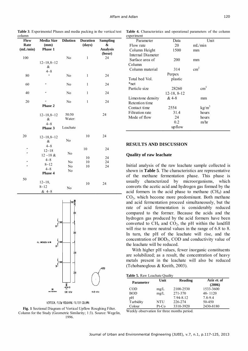
Affam and Adlan
Journal of Urban and Environmental Engineering (JUEE), v.7, n.1, p.117-125, 2013
120
Table 3. Experimental Phases and media packing in the vertical test column
Flow Rate
(mL/min)
Media Size (mm)
Phase 1
Dilution Duration (days)
Sampling &
Analysis (hour)
100 1218,812
& 48
No 1 24
״ 80
No 1 24
60
40
20
20
״ ״ ״ ״
50
״ ״ ״
Phase 2
1218,812 &
48 Phase 3
1218,812
& 48
1218 12 18 &
48 812 48
Phase 4 1218, 812 & 48
No
No
No
50:50 Water: Leachate
No
No
No No No
No
1
1
1
10
10
10 10 10
10
24
24
24
24
24
24
24 24 24
24
Fig. 1 Sectional Diagram of Vertical Upflow Roughing Filter.
Column for the Study (Geometric Similarity; 1:3). Source: Wegelin, 1996.
Table 4. Characteristics and operational parameters of the column experiment
Parameter Data Unit Flow rate Column Height Internal Diameter Surface area of Column Column material Total bed Vol. *net Particle size Limestone density Retention time Contact time Filtration rate Mode of flow
20 1500
200
314
Perpex plastic
28260
12-18, 8-12 & 4-8
2554
31.4 24 0.2
upflow
mL/min mm mm cm2 cm3 mm kg/m3 hours hours m/hr
RESULTS AND DISCUSSION Quality of raw leachate Initial analysis of the raw leachate sample collected is shown in Table 5. The characteristics are representative of the methane fermentation phase. This phase is usually characterized by microorganisms, which converts the acetic acid and hydrogen gas formed by the acid formers in the acid phase to methane (CH4) and CO2, which become more predominant. Both methane and acid fermentation proceed simultaneously, but the rate of acid fermentation is considerably reduced compared to the former. Because the acids and the hydrogen gas produced by the acid formers have been converted to CH4 and CO2, the pH within the landfill will rise to more neutral values in the range of 6.8 to 8. In turn, the pH of the leachate will rise, and the concentration of BOD5, COD and conductivity value of the leachate will be reduced.
With higher pH values, fewer inorganic constituents are solubilized; as a result, the concentration of heavy metals present in the leachate will also be reduced (Tchobanoglous & Kreith, 2003). Table 5. Raw Leachate Quality
Parameter Unit
Reading
Aziz et. al
(2006)
COD BOD pH Turbidity Colour
mg/L mg/L NTU Pt-Co
2100-2530 271-370 7.94-8.12 226-274 3310-3920
1533-3600 48- 1120 7.8-9.4 50-450 2430-8180
Weekly observation for three months period.
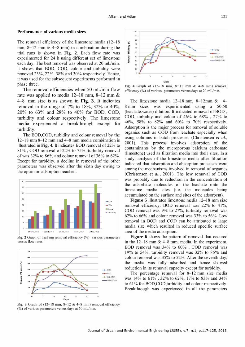
Affam and Adlan
Journal of Urban and Environmental Engineering (JUEE), v.7, n.1, p.117-125, 2013
121
Performance of various media sizes The removal efficiency of the limestone media (12–18 mm, 812 mm & 48 mm) in combination during the trial runs is shown in Fig. 2. Each flow rate was experimented for 24 h using different set of limestone each day. The best removal was observed at 20 mL/min. It shows that BOD, COD, colour and turbidity were removed 23%, 22%, 38% and 30% respectively. Hence, it was used for the subsequent experiments performed in phase three.
The removal efficiencies when 50 mL/min flow rate was applied to media 12–18 mm, 8–12 mm & 4–8 mm size is as shown in Fig. 3. It indicates removal in the range of 7% to 18%, 32% to 40%, 20% to 63% and 28% to 40% for BOD, COD, turbidity and colour respectively. The limestone media experienced a breakthrough except for turbidity.
The BOD,COD, turbidity and colour removal by the 12–18 mm 8–12 mm and 4–8 mm media combination is illustrated in Fig. 4. It indicates BOD removal of 22% to 81% , COD removal of 22% to 75%, turbidity removal of was 32% to 86% and colour removal of 36% to 62%. Except for turbidity, a decline in removal of the other parameters was observed after the sixth day owing to the optimum adsorption reached.
Fig. 2 Graph of trial run removal efficiency (%) various parameters versus flow rates.
Fig. 3 Graph of (1218 mm, 812 & 48 mm) removal efficiency (%) of various parameters versus days at 50 mL/min.
Fig. 4 Graph of (12–18 mm, 812 mm & 4–8 mm) removal efficiency (%) of various parameters versus days at 20 mL/min.
The limestone media 12–18 mm, 812mm & 4–8 mm sizes was experimented using a 50:50 (leachate:water) dilution. It indicated removal of BOD , COD, turbidity and colour of 46% to 68% , 27% to 46%, 58% to 82% and 60% to 70% respectively. Adsorption is the major process for removal of soluble organics such as COD from leachate especially when using columns in batch processes (Christensen et al., 2001). This process involves adsorption of the contaminants by the microporous calcium carbonate (limestone) used as filtration media into their sites. In a study, analysis of the limestone media after filtration indicated that adsorption and absorption processes were among the mechanisms involved in removal of organics (Christensen et al., 2001). The low removal of COD was probably due to reduction in the concentration of the adsorbate molecules of the leachate onto the limestone media sites (i.e. the molecules being accumulated on the surface and sites of the adsorbent).
Figure 5 illustrates limestone media 12–18 mm size removal efficiency. BOD removal was 22% to 41%, COD removal was 9% to 27%, turbidity removal was 62% to 66% and colour removal was 33% to 56%. Low removal in BOD and COD can be attributed to large media size which resulted in reduced specific surface area of the media adsorption. Figure 6 shows the pattern of removal that occured in the 12–18 mm & 4–8 mm, media. In the experiment, BOD removal was 34% to 60% , COD removal was 19% to 54%, turbidity removal was 32% to 86% and colour removal was 35% to 52%. After the seventh day, the media was fully adsorbed and hence showed reduction in its removal capacity except for turbidity.
The percentage removal for 8–12 mm size media was 14% to 61% , 32% to 62%, 17% to 83% and 34% to 61% for BOD,COD,turbidity and colour respectively. Breakthrough was experienced in all the parameters
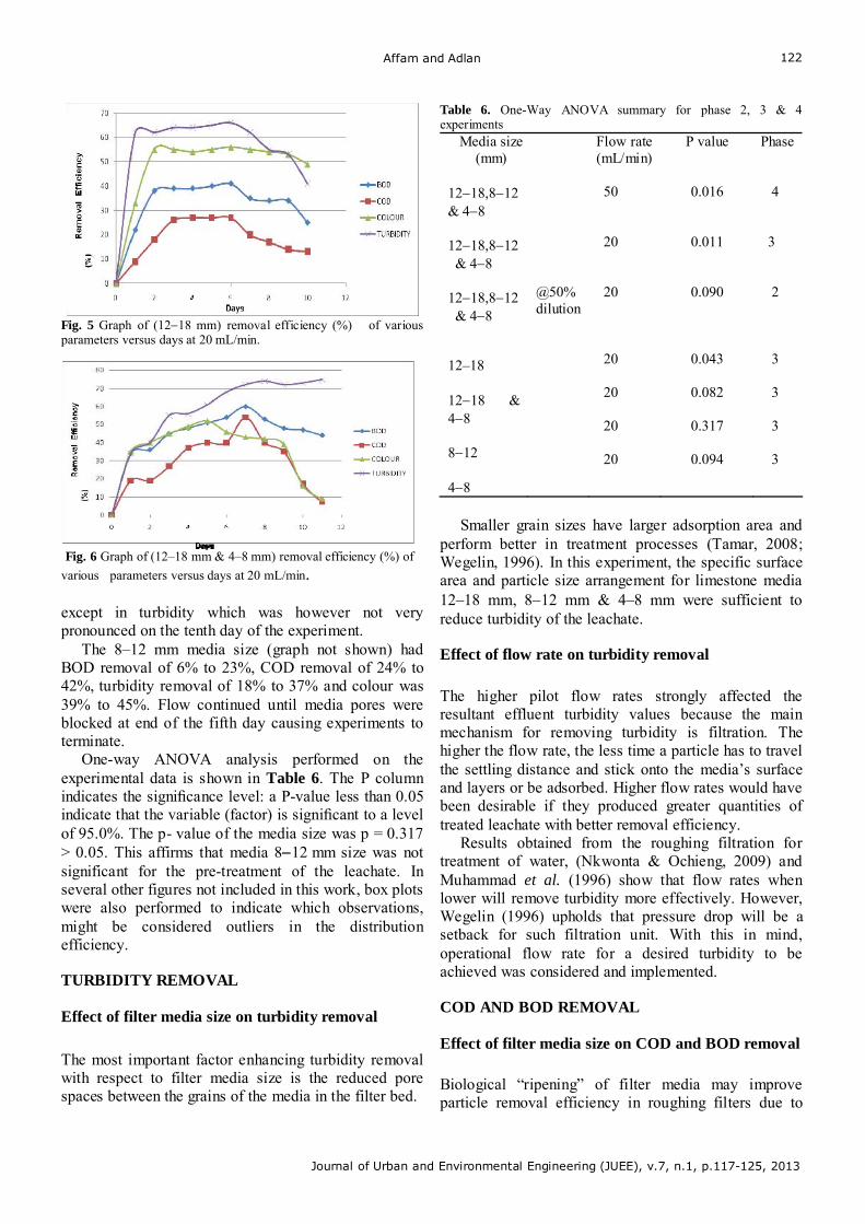
Affam and Adlan
Journal of Urban and Environmental Engineering (JUEE), v.7, n.1, p.117-125, 2013
122
Fig. 5 Graph of (1218 mm) removal efficiency (%) of various parameters versus days at 20 mL/min.
Fig. 6 Graph of (12–18 mm & 4–8 mm) removal efficiency (%) of
various parameters versus days at 20 mL/min. except in turbidity which was however not very pronounced on the tenth day of the experiment.
The 8–12 mm media size (graph not shown) had BOD removal of 6% to 23%, COD removal of 24% to 42%, turbidity removal of 18% to 37% and colour was 39% to 45%. Flow continued until media pores were blocked at end of the fifth day causing experiments to terminate.
One-way ANOVA analysis performed on the experimental data is shown in Table 6. The P column indicates the significance level: a P-value less than 0.05 indicate that the variable (factor) is significant to a level of 95.0%. The p- value of the media size was p = 0.317 > 0.05. This affirms that media 812 mm size was not significant for the pre-treatment of the leachate. In several other figures not included in this work, box plots were also performed to indicate which observations, might be considered outliers in the distribution efficiency.
TURBIDITY REMOVAL
Effect of filter media size on turbidity removal
The most important factor enhancing turbidity removal with respect to filter media size is the reduced pore spaces between the grains of the media in the filter bed.
Table 6. One-Way ANOVA summary for phase 2, 3 & 4 experiments
Media size (mm)
Flow rate (mL/min)
P value
Phase
1218,812 & 48 1218,812 & 48 1218,812 & 48 12–18 1218 & 48 812 48
@50% dilution
50 20 20 20 20 20 20
0.016
0.011
0.090
0.043 0.082
0.317
0.094
4 3 2 3 3 3 3
Smaller grain sizes have larger adsorption area and
perform better in treatment processes (Tamar, 2008; Wegelin, 1996). In this experiment, the specific surface area and particle size arrangement for limestone media 12–18 mm, 812 mm & 4–8 mm were sufficient to reduce turbidity of the leachate.
Effect of flow rate on turbidity removal
The higher pilot flow rates strongly affected the resultant effluent turbidity values because the main mechanism for removing turbidity is filtration. The higher the flow rate, the less time a particle has to travel the settling distance and stick onto the media’s surface and layers or be adsorbed. Higher flow rates would have been desirable if they produced greater quantities of treated leachate with better removal efficiency.
Results obtained from the roughing filtration for treatment of water, (Nkwonta & Ochieng, 2009) and Muhammad et al. (1996) show that flow rates when lower will remove turbidity more effectively. However, Wegelin (1996) upholds that pressure drop will be a setback for such filtration unit. With this in mind, operational flow rate for a desired turbidity to be achieved was considered and implemented.
COD AND BOD REMOVAL
Effect of filter media size on COD and BOD removal
Biological “ripening” of filter media may improve particle removal efficiency in roughing filters due to
Affam and Adlan
Journal of Urban and Environmental Engineering (JUEE), v.7, n.1, p.117-125, 2013
123
increased stickiness of filter media (Collins et al., 1994). Exposure of the media to sunlight was avoided to minimize potential errors which can be introduced by biological activity into the column. To evaluate the potential in removal of BOD and COD, the experiment was non-recycle and upon final use of the media it was observed to be very sticky by means of touching. In addition, media 48 mm, 812 mm and 1218 mm size had a higher removal as against 812 mm, 48 mm alone and other combinations. This could be as a result of increased surface area and hence adsorption sites. This could be similar to Wegelin (1996) slow sand filtration experiments where removal of pathogens was by the sedimentation or deposition and effective settling of particles on the grains of the media. Thus, COD and BOD5 are possible to be reduced from leachate by limestone media.
Effect of flow rate on COD and BOD removal
The flow rate which removed optimum COD and BOD was observed to be 20ml/L. This was obvious when higher flow rates indicated lower removal of COD and BOD. However, a more critical factor that can be attributed to the low removal was the media saturation point that must have been reached. Lower flow rate allows an increased pathogen removal, which is especially important in colder climates where biological activity is more time dependent (Huisman & Wood, 1974; Wegelin, 1996; Nkwonta & Ochieng, 2009). Recent research carried out by Jenkins et al. (2009) on intermittently-operated sand filters has highlighted the importance of sand size and hydraulic loading both of which directly affect microbiological removal. However, it is possible to increase the filtration rate if effective pretreatment has been given and if an effective disinfection stage follows after filtration (Ellis, 1987).
COLOUR REMOVAL
Effect of flow rate on colour removal
A report observed that colour removal was poor when higher filtration rates were applied in continually-operated sand filters, although the filtrate quality remained reasonably good (Muhammad et al., 1996). In this study, it was justified and reasonable to apply lower flow rates for optimum removal to be obtained. The limestone media was not capable of removing the colour from the leachate. It would therefore require a chemical or biological treatment for effective removal of colour.
Effect of filter media size on colour removal
The removal of dissolved colour or true colour by varying filter media size in roughing filtration has not been properly documented. Since, colour is related to humic substances, it is expected that true colour exists in relatively stable suspension and it is more difficult to remove. Collins et al. (1994) reported that removal of true colour in roughing filters compares favourably to that achieved by slow sand filtration. Wegelin (1996) observed true colour removal in the range of 20 to 50 %. There has been numerous reports of removal of apparent colour, which is the colour attributed to undissolved particulate matter. Wolters et al. (1989) and Barret (1989) both found removal of apparent colour to be 45 to 80 %. In this study, the optimum true colour removal was 62% using the media 12–18 mm, 812 mm & 48 mm size combination.
Length of run time on removal efficiencies
The length of run for each set of media combination study was ten days. The limestone media experienced an average breakthrough in a period of six days as found from the laboratory experiments. The length of run was basically dependent on the performance of the media in terms of its removal and adsorption capacity. In each study, when breakthrough was experienced the experiment was terminated.
pH Change during the roughing filtration process
During the roughing filtration treatment the pH showed a little variation. The raw leachate sample was between pH 7.94 and pH 8.12 but increased to pH 8.42 after filtration. This is due to the presence of CO3 in limestone (Aziz et al., 2004) an unstable oxide of carbon and declined as removal efficiency reduced. The dissolution of calcium carbonate can increase the concentration of alkalinity.
Headloss during length of run time The headloss was also considered in this study. Although, the main essence of conducting the research was to ascertain the effectiveness of the limestone media in pre-treatment of leachate, a documentary of the headloss during each run time for every media combination was randomly done. To affirm the postulation by Boller & Kavanaugh (1995) which demonstrated that the rate of headloss build-up in a granular media filter, for a constant mass of solids being removed, is strongly dependent on the size of the particulates in suspension and the size of the granular media. In addition, the principal cause of the rapid
Affam and Adlan
Journal of Urban and Environmental Engineering (JUEE), v.7, n.1, p.117-125, 2013
124
increase in headloss observed for smaller particles in many filtration studies is due to the nature of the aggregation or deposition process inside the pore spaces of the porous media. Observations during this experiment indicated that maximum headloss was 0.5 cm at 20 mL/min flow rate. According to Amin & Aziz (2002), negative heads do not occur in the upflow vertical roughing filter bed, however a crack occurs at the bottom layers of filter bed, when headloss reaches maximum. It is noteworthy that, during the filtration treatment process for media 4–8 mm size, there was an entire blockage and flow stopped abruptly.
CONCLUSION
The optimum removal efficiency of BOD, COD, colour and turbidity using the limestone media in the vertical upflow roughing filter stacked with 1218 mm, 812 mm and 48 mm size from bottom towards the top of the column at 20 mL/min and with no dilution of leachate was 81%, 75%, 62% and 86%, respectively. During the 50:50 water-leachate dilutions, colour removal was 70 %.
Increasing filtration rate and reducing contact
time simultaneously reduced adsorption and hence removal efficiency.
The vertical upflow roughing filter can be used
for pre-treatment or polishing of leachate before further biological treatment.
Acknowledgement The authors are thankful to the management of the Universiti Sains Malaysia (USM) for providing facilities for this research.
REFERENCES
American Public Health Association, APHA. (1998) Standard methods for examination of water and wastewater, 20th ed. Washington, D.C. USA.
American Public Health Association, APHA. (1992) Standard methods for examination of water and wastewater, 19th ed. Washington, D.C. USA.
Amin, K.N., Aziz, S.Q. (2002) Pressure distribution in filter media in conventional filters. Journal of Dohuk University, Vol.5, No.2, 56-59.
Aziz, H. A., Salina A., Mohd. N. A., Faridah, Asaari A.H., Zahari, M.S. (2006) Colour removal from landfill leachate by coagulation and flocculation processes, Bioresource Technology 98, 218–220.
Aziz, H.A., Yusoff M.S., Mohd N.A., Adnan N.H., Salina, A. (2004) Physico-chemical removal of iron from semi-aerobic landfill leachate by limestone filter. Waste Management 24, 353–358.
Aziz, H.A., Othman, N., Yusuff, M.S., Basri, D.R.H., Asaari, F.A.H., Adlan, M.N., Othman, F., Johari, M., Perwira, M. (2001) Removal of copper from water using limestone filtration technique-determination of mechanism of removal. Environment International 26, 395–399.
Barrett, J.M. (1989) Improvement of slow sand filtration of warm water by using coarse sand. Ph.D Thesis, University of Colorado, USA.
Boller, M.A., Kavanaugh, M.C. (1995) Particle characteristics and headloss increase in granular media filtration. Water Research, Vol. 29, Issue 4, 1139-1149.
Boller, M. (1993) Filter mechanisms in roughing filters. Journal of Water Supply Research and Technology - Aqua, Vol. 42, 174-185.
Collins, M.R., Westersund C., Cole J., Roccaro J. (1994) Evaluation of roughing filtration design variables. AWWARF and AWWA, Denver, USA. 77- 88.
Cooney, D.O. (1999) Adsorption design for wastewater treatment. CRC Press LLC, Florida, USA.
Ellis, K.V. (1987) Slow sand filtration as a technique for the tertiary treatment of municipal sewages. Water Research, Vol. 21, 403-410
Galvis, G., Visscher, J.T., Latorre J. (1998) Multi-stage filtration and innovation water treatment technology. International reference centre for community water supply and sanitation, The Hague, Netherlands and Universidad del valle instituto Cinara, Cali, Colombia.
Ghaly, A.E., Kamal, M.A., Mahmoud, N.S., Cote. R. (2007) Treatment of landfill leachate using limestone/sandstone filters under aerobic batch conditions. American Journal of Environmental Sciences 3 (2), 43-53.
Huisman, L., Wood, W.E. (1974) Slow sand filtration. W.H.O. Geneva, Switzerland. 44.
Jenkins, M.W., Tiwari, S.K., Darby, J., Nyakash, D., Saenyi, W., Langenbach, K. (2009) The biosand filter for improved drinking water quality in high risk communities in the Njoro watershed, Kenya. Research brief, SUMAWA, Global livestock collaborative research support program. University of California, Davis, USA.
Mohd .N.A., Aziz H.A., Maung H.T., Hung. Y. (2008) Performance of horizontal flow roughing filter using limestone media for the removal of turbidity, suspended solids, biochemical oxygen demand and coliform organisms from wastewater, International Journal of Environment and Waste Management, Vol. 2, No.3, 203 – 214.
Muhammad, N., Ellis K., Parr, J., Smith, M.D. (1996) Optimization of slow sand filtration. Reaching the unreached: challenges for the 21st century. 22nd WEDC conference New Delhi, India. 283 - 285.
Christensen, T.H., Kdelsen, P., Bjerg, P.L., Christensen, J.B., Baun, A., Albrech, H. Biogeocemistry of landfill leachate- review.
(2001) Appled Geochemistry 16, 659-718. Nkwonta, O.I., Ochieng, G.M. (2009) Passive treatment of mine
water using roughing filters as a pre-treatment option. Abstracts of the international mine water conference, Cilla Taylor Conference, Pretoria, South Africa. 359-365
Nkwonta, O.I., Ochieng, G.M. (2009) Roughing filter for water pre-treatment technology in developing countries: A review. International Journal of Physical Sciences, Vol. 4 (9), 455-463.
Nkwonta O. (2010) A comparison of horizontal roughing filters and vertical roughing filters in wastewater treatment using gravel as a filter media. International Journal of the Physical Sciences. Vol. 5(8), 1240-1247.
Onay, T. T., Pohland, F.G. (1998) In situ nitrogen management in controlled bioreactor landfills. Water Resources, Vol. 32, No. 5. 1383-1392.

Affam and Adlan
Journal of Urban and Environmental Engineering (JUEE), v.7, n.1, p.117-125, 2013
125
Oasim, S.R., Chiang, W. (1994) Sanitary landfill leachate-generation, control and treatment Technomic Publishing Co. Inc. Texas, USA.
Reinhart, D.R., Townsend T.G. (1998) Landfill bioreactor design and operation, CRC Press LLC: Boca Raton, Florida. USA.
Smith, K.S., Plumlee, G.S., Ficklin, W.H. (1994) Predicting water contamination from metal mines and mining wastes. International land reclamation and mine drainage conference and third international conference on the abatement of acidic drainage. U.S. geological survey, report No. 94-264.
Sun, Q. (2004) Iron and acid removal from acid mine drainage in open limestone systems. PhD dissertation. Retrieved from: https: //etd.wvu.edu/ etd/controller.jsp?moduleName=document data&jsp_etdId=1315
Tchobanoglous, G., Kreith, F. (2003) Handbook of solid waste management, second ed. McGraw-Hill Inc, New York, USA.
Tchobanoglous, G., Franklin, B.H., Stensel, D. (2003) Wastewater engineering: Treatment and reuse, fourth edition. Metcalf & Eddy, Inc. USA.
Wegelin, M. (1996) Surface water treatment by roughing filters. A Design, construction and operation manual. SANDEC report No. 2/96. Switzerland.
Wolters, H., Smet, J.E.M., Galvis, J. (1989) Pre-treatment methods for community water supply. Ch.8, IRC, International water and sanitation centre, Netherlands.
Xu, C.Y., Schwartz F.W., Traina, S.J. (1997) Treatment of acid-mine water with calcite and quartz sand. Environmental Engineering Science, 14, 141-152.
Quentin B., 2010. Lean six sigma and Minitab: The Complete Toolbox Guide for All Lean Six Sigma Practitioners (3rd Ed.) OPEX Resources Ltd, United Kingdom.
Deb, Gupta and Misra
Journal of Urban and Environmental Engineering (JUEE), v.7, n.1, p.126-133, 2013
126
Journal of Urban and Environmental Engineering, v.7, n.1, p.126-133
Journal of Urban and Environmental Engineering
UEEJ ISSN 1982-3932
doi: 10.4090/juee.2013.v7n1.126133 www.journal-uee.org
PERFORMANCE ANALYSIS OF A HELICAL SAVONIUS ROTOR WITHOUT SHAFT AT 45° TWIST ANGLE USING CFD
Bachu Deb1, Rajat Gupta2 and R.D. Misra3
1 Department of Mechanical Engineering, NIT Silchar, Silchar - 788010, Assam, India 2 National Institute Technology Srinagar
3 Department of Mechanical Engineering, NIT Silchar
Received 28 December 2012; received in revised form 30 January 2013; accepted 09 February 2013
Abstract: Helical Savonius rotor exhibits better performance characteristics at all the rotor angles
compared to conventional Savonius rotor. However studies related to the performance measurement and flow physics of such rotor are very scarce. Keeping this in view, in this paper, a three dimensional Computational Fluid Dynamics analysis using commercial Fluent 6.2 software was done to predict the performance of a two-bucket helical Savonius rotor without shaft and with end plates in a complete cycle of rotation. A two-bucket helical Savonius rotor having height of 60 cm and diameter of 17 cm with 45° bucket twist angle was designed using Gambit. The buckets were connected at the top and bottom circular end plates, which are 1.1 times the rotor diameter. The k-ε turbulence model with second order upwind discretization scheme was adopted with standard wall condition. Power coefficients (Cp) and torque coefficients (Ct) at different tip speed ratios were evaluated at different rotor angles. From the investigation, it was observed that power coefficient increased with increase of tip speed ratio up to an optimum limit, but then decreased even further tip speed ratio was increased. Further investigation was done on the variations of Cp & Ct in a complete cycle of rotation from 0° to 360° in a step of 45° rotor corresponding to the optimum tip speed ratio. The value of Cp at all the rotor angles is positive. Moreover, velocity magnitude contours were analyzed for each rotor angle and it could be concluded that high aerodynamic torque and power can be expected when the rotor is positioned at 45º & 90º with respect to incoming flow.
Keywords:
Two-bucket helical Savonius rotor; tip speed ratio; power coefficient; torque coefficient.
© 2013 Journal of Urban and Environmental Engineering (JUEE). All rights reserved.
Correspondence to: Bachu Deb. E-mail: [email protected]
Deb, Gupta and Misra
Journal of Urban and Environmental Engineering (JUEE), v.7, n.1, p.126-133, 2013
127
INTRODUCTION
The Savonius vertical axis wind rotor was first developed by S. J. Savonius in 1929 (Savonius, 1931). The design was based on the principle of Flettner’s rotor. He used a rotor which was formed by cutting a Flettner cylinder from top to bottom and then moving the two semi-cylinder surfaces sideways along the cutting plane so that the cross-section resembled the letter ‘S’. To determine the best geometry, Savonius tested 30 different models in the wind tunnel as well as in the open air. The best of his rotor model had 31% efficiency and the maximum efficiency of the prototype in the natural wind was 37%. Bach (1031) made some investigations of the S-rotor and related machines. The highest measured efficiency was 24%.
McPherson (1972) reported a highest efficiency of 33% and the maximum power coefficient obtained by Newman (1974) was only 20%. Modi et al. (1984) reported a power coefficient of 0.22.There had been some works done as to incorporate some modifications in the design of blades so that Savonius rotor may be quite useful for small-scale power requirements. In the last few decades many researchers had worked on the different designs of Savonius rotor and obtained its efficiency in the range of 15%38%. In the Continuation Grinspan et al. (2001) in this direction led to the development of a new blade shape with a twist for the Savonius rotor. They reported a maximum power coefficient of 0.5. Further Saha et al. (1994) performed experiments on twist bladed Savonius rotor made of bamboo in a low-speed wind tunnel. They showed that their model was independent of wind direction and though the model produced slightly lower rotational speed but easy fabrication of such models made their design suitable for small-scale requirements. Further such design can worth hundred times better than those using deflecting plates & shielding to increase efficiency, which would make the design structurally complex. Again Saha & Rajkumar (2008) performed work on twist bladed metallic S-rotor and compared the performance with conventional semicircular blades having no twist. They obtain Cp of 0.14, which was higher than that of the later with Cp of 0.11. The rotor also produced starting torque and larger rotational speeds. The analysis is done by Hussain et al. (2008) on the enhancement of efficiency by modifying the blade configuration from straight semi circular to a twisted semi circular one. The twist in this turbine is assumed to be given as the bottom cross-sectional surface of the blades is fixed and the top cross-sectional surface is given the desired twist with respect to the bottom fixed surface. Wind flow analysis is done over each configuration of the rotor with the blade twist angles
ranging from 5o to 60o in steps of 5o. The optimum angle of twist at which the efficiency and the output power is maximum is evaluated.
Biswas & Gupta (2007) conducted model tests on three-bucket S-rotor, taking tunnel blockage into consideration, and reported maximum power coefficient of 38%. Further Bhaumik & Gupta (2010) studied experimentally the performance of helical Savonius rotor at 45º twist angle in a centrifugal blower. They consider the provision of different overlap ratio from 0.106 to 0.186.It is concluded from their result that maximum Cp is obtained as 0.421 at an overlap ratio of 0.147. Gupta & Deb (2011) studied the CFD analysis of a two bucket helical Savonius rotor with shaft at 45º twist angle. From their study they concluded that the highest values of dynamic pressure and velocity magnitude were obtained at the chord ends with 450
bucket twist and 900 rotor angle, which would ensure improved performance of the rotor as a whole by increasing the aerodynamic torque production of the rotor. Kamoji et al. (2008) investigates single stages modified Savonius rotorsand concluded that at overlap ratio 0.0 blade arc angle 124º and an aspect ratio of 0.7 has a maximum coefficient of power at a Reynolds number of 1 500 000 which is higher than conventional Savonius rotor.
Keeping this in view, a two-bucket helical savonius rotor without shaft having 45° bucket twist angle was designed. Computational fluid dynamics (CFD) analysis using fluent package was done to analyse the power coefficient and torque coefficient of the rotor at 45° blade twist angle at different rotor angles. Further velocity magnitude contours were analyzed to understand the flow physics of the rotor at different rotor angles.
PHYSICAL MODEL The three-dimensional model of the two-bucket helical Savonius rotor without shaft at 45° twist angle is shown in Fig. 1.The bucket are connected at the top and bottom circular end plates, which is 1.1 times the rotor diameter. There is no central shaft in between the top and bottom plates. Both the inner edge and the outer edge undergo a twist of 45°, a quarter pitch turn. The blade retains its semi-circular cross section from the bottom (0°) to the top (45°). The buckets were spaced 180° apart and were fixed to the end plates. The physical models were designed for five rotor angles namely 0°, 45°, 90°, 135° and 180°. The height of the rotor (H) is 60 cm, radius of the bucket (R) is 8.5 cm, and diameter of the shaft (d) is 3.5 cm.
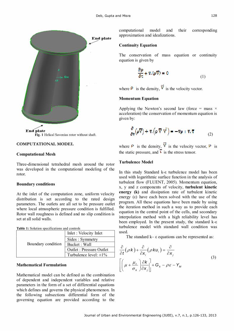
Deb, Gupta and Misra
Journal of Urban and Environmental Engineering (JUEE), v.7, n.1, p.126-133, 2013
128
Fig. 1 Helical Savonius rotor without shaft.
COMPUTATIONAL MODEL Computational Mesh Three-dimensional tetrahedral mesh around the rotor was developed in the computational modeling of the rotor.
Boundary conditions At the inlet of the computation zone, uniform velocity distribution is set according to the rated design parameters. The outlets are all set to be pressure outlet where local atmospheric pressure condition is fulfilled. Rotor wall roughness is defined and no slip condition is set at all solid walls. Table 1: Solution specifications and controls
Inlet : Velocity Inlet
Sides : Symmetry Bucket : Wall Outlet : Pressure Outlet
Boundary condition
Turbulence level: ±1%
Mathematical Formulation Mathematical model can be defined as the combination of dependent and independent variables and relative parameters in the form of a set of differential equations which defines and governs the physical phenomenon. In the following subsections differential form of the governing equation are provided according to the
computational model and their corresponding approximation and idealizations.
Continuity Equation The conservation of mass equation or continuity equation is given by
(1)
where is the density, is the velocity vector. Momentum Equation Applying the Newton’s second law (force = mass × acceleration) the conservation of momentum equation is given by:
(2)
where is the density, is the velocity vector, is the static pressure, and is the stress tensor.
Turbulence Model In this study Standard k-ε turbulence model has been used with logarithmic surface function in the analysis of turbulent flow (FLUENT, 2005). Momentum equation, x, y and z components of velocity, turbulent kinetic energy (k) and dissipation rate of turbulent kinetic energy (ε) have each been solved with the use of the program. All these equations have been made by using the iteration method in such a way as to provide each equation in the central point of the cells, and secondary interpolation method with a high reliability level has been employed. In the present study, the standard k-ε turbulence model with standard wall condition was used.
The standard k– ε equations can be represented as:
ii j
tk M
k j
k kut x x
kG Y
x
(3)
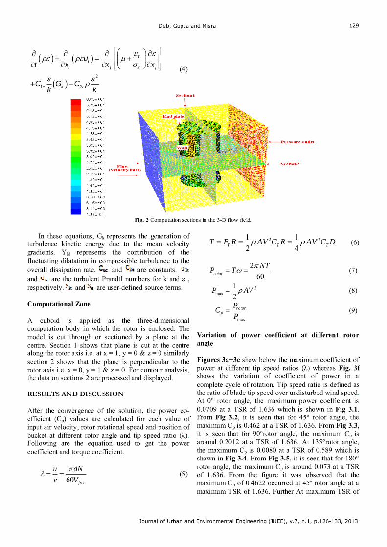
Deb, Gupta and Misra
Journal of Urban and Environmental Engineering (JUEE), v.7, n.1, p.126-133, 2013
129
2
1 2
ti
i j j
k
ut x x x
C G Ck k
(4)
Fig. 2 Computation sections in the 3-D flow field.
In these equations, Gk represents the generation of
turbulence kinetic energy due to the mean velocity gradients. YM represents the contribution of the fluctuating dilatation in compressible turbulence to the overall dissipation rate. and are constants. and are the turbulent Prandtl numbers for k and ε , respectively. and are user-defined source terms.
Computational Zone A cuboid is applied as the three-dimensional computation body in which the rotor is enclosed. The model is cut through or sectioned by a plane at the centre. Section 1 shows that plane is cut at the centre along the rotor axis i.e. at x = 1, y = 0 & z = 0 similarly section 2 shows that the plane is perpendicular to the rotor axis i.e. x = 0, y = 1 & z = 0. For contour analysis, the data on sections 2 are processed and displayed. RESULTS AND DISCUSSION After the convergence of the solution, the power co-efficient (Cp) values are calculated for each value of input air velocity, rotor rotational speed and position of bucket at different rotor angle and tip speed ratio (λ). Following are the equation used to get the power coefficient and torque coefficient.
60 free
u dN
v V
(5)
2 21 1
2 4T T TT F R AV C R AV C D (6)
2
60rotor
NTP T
(7)
3max
1
2P AV (8)
max
rotorP
PC
P (9)
Variation of power coefficient at different rotor angle Figures 3a−3e show below the maximum coefficient of power at different tip speed ratios (λ) whereas Fig. 3f shows the variation of coefficient of power in a complete cycle of rotation. Tip speed ratio is defined as the ratio of blade tip speed over undisturbed wind speed. At 0° rotor angle, the maximum power coefficient is 0.0709 at a TSR of 1.636 which is shown in Fig 3.1. From Fig 3.2, it is seen that for 45° rotor angle, the maximum Cp is 0.462 at a TSR of 1.636. From Fig 3.3, it is seen that for 90°rotor angle, the maximum Cp is around 0.2012 at a TSR of 1.636. At 135°rotor angle, the maximum Cp is 0.0080 at a TSR of 0.589 which is shown in Fig 3.4. From Fig 3.5, it is seen that for 180° rotor angle, the maximum Cp is around 0.073 at a TSR of 1.636. From the figure it was observed that the maximum Cp of 0.4622 occurred at 45º rotor angle at a maximum TSR of 1.636. Further At maximum TSR of
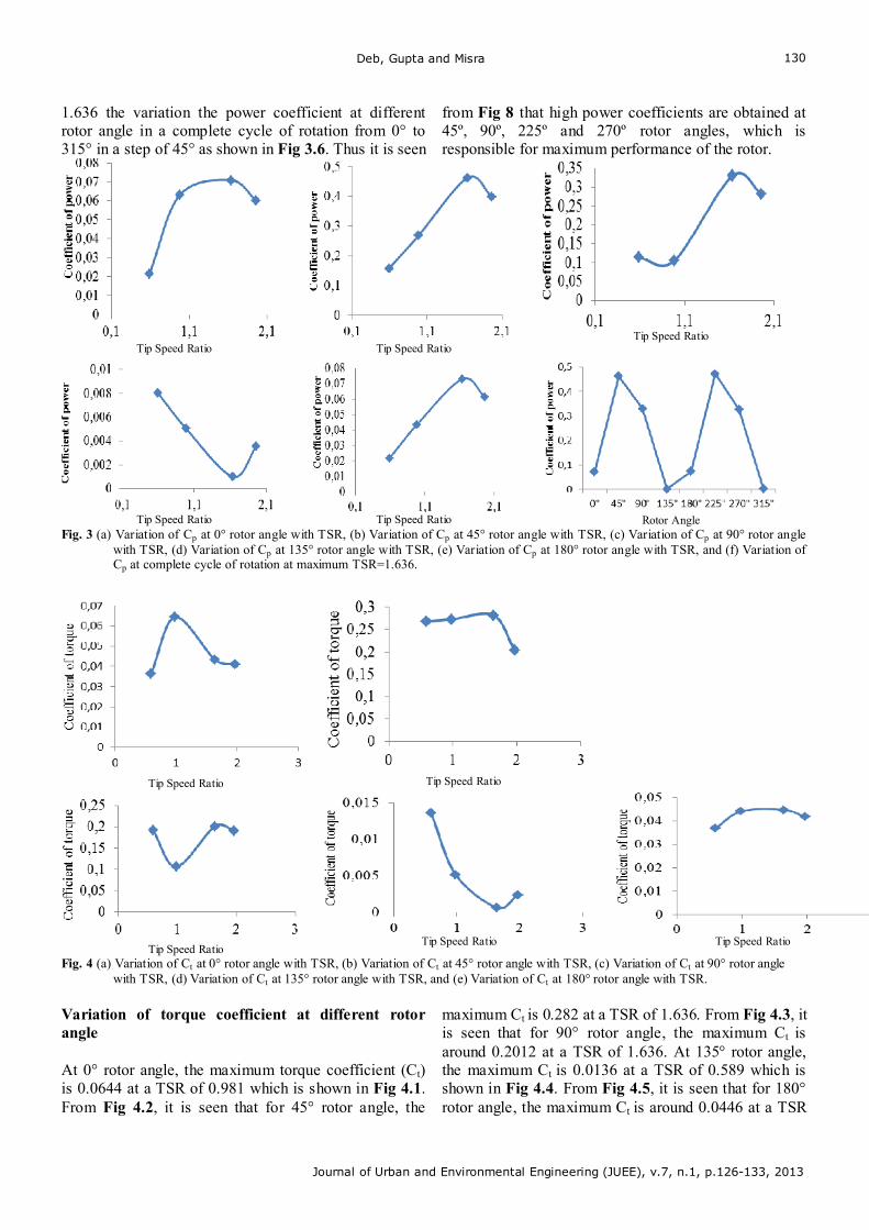
Deb, Gupta and Misra
Journal of Urban and Environmental Engineering (JUEE), v.7, n.1, p.126-133, 2013
130
1.636 the variation the power coefficient at different rotor angle in a complete cycle of rotation from 0° to 315° in a step of 45° as shown in Fig 3.6. Thus it is seen
from Fig 8 that high power coefficients are obtained at 45º, 90º, 225º and 270º rotor angles, which is responsible for maximum performance of the rotor.
Tip Speed Ratio
Tip Speed Ratio
Tip Speed Ratio
Tip Speed Ratio
Tip Speed Ratio
Rotor Angle
Fig. 3 (a) Variation of Cp at 0° rotor angle with TSR, (b) Variation of Cp at 45° rotor angle with TSR, (c) Variation of Cp at 90° rotor angle with TSR, (d) Variation of Cp at 135° rotor angle with TSR, (e) Variation of Cp at 180° rotor angle with TSR, and (f) Variation of Cp at complete cycle of rotation at maximum TSR=1.636.
Tip Speed Ratio
Tip Speed Ratio
Tip Speed Ratio
Tip Speed Ratio Tip Speed Ratio
Fig. 4 (a) Variation of Ct at 0° rotor angle with TSR, (b) Variation of Ct at 45° rotor angle with TSR, (c) Variation of Ct at 90° rotor angle with TSR, (d) Variation of Ct at 135° rotor angle with TSR, and (e) Variation of Ct at 180° rotor angle with TSR.
Variation of torque coefficient at different rotor angle At 0° rotor angle, the maximum torque coefficient (Ct) is 0.0644 at a TSR of 0.981 which is shown in Fig 4.1. From Fig 4.2, it is seen that for 45° rotor angle, the
maximum Ct is 0.282 at a TSR of 1.636. From Fig 4.3, it is seen that for 90° rotor angle, the maximum Ct is around 0.2012 at a TSR of 1.636. At 135° rotor angle, the maximum Ct is 0.0136 at a TSR of 0.589 which is shown in Fig 4.4. From Fig 4.5, it is seen that for 180° rotor angle, the maximum Ct is around 0.0446 at a TSR
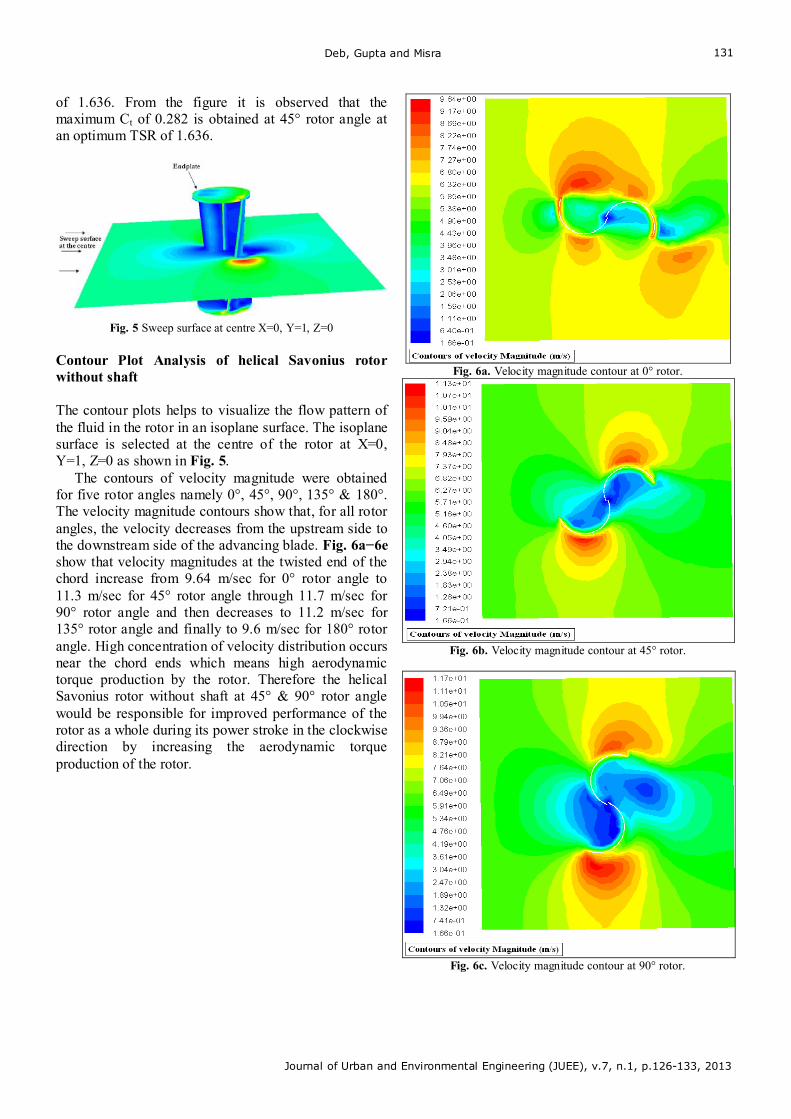
Deb, Gupta and Misra
Journal of Urban and Environmental Engineering (JUEE), v.7, n.1, p.126-133, 2013
131
of 1.636. From the figure it is observed that the maximum Ct of 0.282 is obtained at 45° rotor angle at an optimum TSR of 1.636.
Fig. 5 Sweep surface at centre X=0, Y=1, Z=0
Contour Plot Analysis of helical Savonius rotor without shaft
The contour plots helps to visualize the flow pattern of the fluid in the rotor in an isoplane surface. The isoplane surface is selected at the centre of the rotor at X=0, Y=1, Z=0 as shown in Fig. 5.
The contours of velocity magnitude were obtained for five rotor angles namely 0°, 45°, 90°, 135° & 180°. The velocity magnitude contours show that, for all rotor angles, the velocity decreases from the upstream side to the downstream side of the advancing blade. Fig. 6a−6e show that velocity magnitudes at the twisted end of the chord increase from 9.64 m/sec for 0° rotor angle to 11.3 m/sec for 45° rotor angle through 11.7 m/sec for 90° rotor angle and then decreases to 11.2 m/sec for 135° rotor angle and finally to 9.6 m/sec for 180° rotor angle. High concentration of velocity distribution occurs near the chord ends which means high aerodynamic torque production by the rotor. Therefore the helical Savonius rotor without shaft at 45° & 90° rotor angle would be responsible for improved performance of the rotor as a whole during its power stroke in the clockwise direction by increasing the aerodynamic torque production of the rotor.
Fig. 6a. Velocity magnitude contour at 0° rotor.
Fig. 6b. Velocity magnitude contour at 45° rotor.
Fig. 6c. Velocity magnitude contour at 90° rotor.
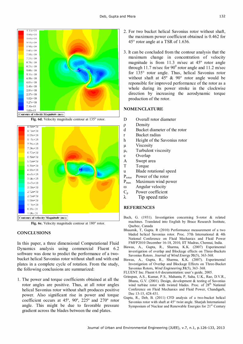
Deb, Gupta and Misra
Journal of Urban and Environmental Engineering (JUEE), v.7, n.1, p.126-133, 2013
132
Fig. 6d. Velocity magnitude contour at 135° rotor.
Fig. 6e. Velocity magnitude contour at 180° rotor.
CONCLUSIONS In this paper, a three dimensional Computational Fluid Dynamics analysis using commercial Fluent 6.2 software was done to predict the performance of a two-bucket helical Savonius rotor without shaft and with end plates in a complete cycle of rotation. From the study, the following conclusions are summarized:
1. The power and torque coefficients obtained at all the
rotor angles are positive. Thus, at all rotor angles helical Savonius rotor without shaft produces positive power. Also significant rise in power and torque coefficient occurs at 45º, 90º, 225º and 270º rotor angle. This might be due to favorable pressure gradient across the blades between the end plates.
2. For two bucket helical Savonius rotor without shaft, the maximum power coefficient obtained is 0.462 for 45° rotor angle at a TSR of 1.636.
3. It can be concluded from the contour analysis that the
maximum change in concentration of velocity magnitude is from 11.3 m/sec at 45º rotor angle through 11.7 m/sec for 900 rotor angle and 11.2 m/sec for 135° rotor angle. Thus, helical Savonius rotor without shaft at 45º & 90° rotor angle would be reponsible for improved performance of the rotor as a whole during its power stroke in the clockwise direction by increasing the aerodynamic torque production of the rotor.
NOMENCLATURE D Overall rotor diameter ρ Density d Bucket diameter of the rotor r Bucket radius h Height of the Savonius rotor µ Viscosity µt Turbulent viscosity e Overlap A Swept area T Torque u Blade rotational speed Protor Power of the rotor Pmax Maximum wind power ω Angular velocity Cp Power coefficient λ Tip speed ratio
REFERENCES Bach, G. (1931). Investigation concerning S-rotor & related
machines. Translated into English by Brace Research Institute, Quebec, Canada
Bhaumik, T, Gupta. R (2010) Performance measurement of a two bladed helical Savonius rotor. Proc. 37th International & 4th National Conference on Fluid Mechanics and Fluid Power FMFP2010 December 16-18, 2010, IIT Madras, Chennai, India.
Biswas, A., Gupta, R., Sharma, K.K. (2007) Experimental investigation of overlap and Blockage effects on Three-Buckets Savonius Rotors. Journal of Wind Energy 31(5), 363-368.
Biswas, A., Gupta, R., Sharma, K.K. (2007). Experimental Investigation of Overlap and Blockage Effects on Three-Bucket Savonius Rotors, Wind Engineering 31(5), 363–368.
FLUENT Inc. Fluent 6.0 documentation: user’s guide, 2005. Grinspan, A.S., Kumar, P.S., Mahanta, P, Saha, U.K., Rao, D.V.R.,
Bhanu, G.V. (2001). Design, development & testing of Savonius wind turbine rotor with twisted blades. Proc. of 28th National Conference on Fluid Mechanics and Fluid Power, Chandigarh, Dec 13-15, 428-431.
Gupta, R., Deb, B. (2011) CFD analysis of a two-bucket helical Savonius rotor with shaft at 45° twist angle. Sharjah International Symposium of Nuclear and Renewable Energies for 21st Century
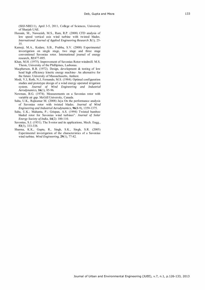
Deb, Gupta and Misra
Journal of Urban and Environmental Engineering (JUEE), v.7, n.1, p.126-133, 2013
133
(SHJ-NRE11), April 3-5, 2011, College of Sciences, University of Sharjah UAE.
Hussain, M., Nawazish, M.S., Ram, R.P. (2008) CFD analysis of low speed vertical axis wind turbine with twisted blades. International Journal of Applied Engineering Research 3(1), 25-35.
Kamoji, M.A., Kedare, S.B., Prabhu, S.V. (2008) Experimental investigation on single stage, two stage and three stage conventional Savonius rotor. International journal of energy research, 32:877-895.
Khan, M.H. (1975). Improvement of Savonius Rotor-windmill. M.S. Thesis, University of the Phillipines, Lasbonas.
Macpherson, R.B. (1972). Design, development & testing of low head high efficiency kinetic energy machine- An alternative for the future. University of Massachusetts, Amhest.
Modi, V.J, Roth, N.J, Fernando, M.S. (1984). Optimal configuration studies and prototype design of a wind energy operated irrigation system. Journal of Wind Engineering and Industrial Aerodynamics, 16(1), 85-96.
Newman, B.G. (1974). Measurements on a Savonius rotor with variable air gap. McGill University, Canada.
Saha, U.K., Rajkumar M. (2008) Jaya On the performance analysis of Savonius rotor with twisted blades. Journal of Wind Engineering and Industrial Aerodynamics, 96(8-9), 1359-1375.
Saha, U.K.; Mahanta, P.; Grispan, A.S. (1994) Twisted bamboo bladed rotor for Savonius wind turbines”. Journal of Solar Energy Society of India, 14(2): 100-110.
Savonius, S.J. (1931). The S-rotor and its applications, Mech. Engg., 53(3), 333-338.
Sharma, K.K., Gupta, R., Singh, S.K., Singh, S.R. (2005) Experimental investigation of the characteristics of a Savonius wind turbine. Wind Engineering, 29(1), 77-82.
Abdel-Rahman, Mohamed, Gad and Hashem
Journal of Urban and Environmental Engineering (JUEE), v.7, n.1, p.134-142, 2013
134
Journal of Urban and Environmental Engineering, v.7, n.1, p.134-142
Journal of Urban and Environmental Engineering
UEEJ ISSN 1982-3932
doi: 10.4090/juee.2013.v7n1.134142 www.journal-uee.org
EFFECTIVENESS OF WASTE STABILIZATION PONDS IN REMOVAL OF LINEAR ALKYL BENZENE SALFONATE (LAS)
Ahmed. M. Abdel-Rahman 1, Ahmed. A. Mohamed2, Ali. A. M. Gad2 and Mohamed
Hashem2
1 M.SC. Researcher, Civil Engineering Department, Faculty of Engineering, Assiut University, Egypt. 2Associate Professor, Civil Engineering Department, Faculty of Engineering, Assiut University, Egypt.
Received 23 February 2013; received in revised form 28 March 2013; accepted 17 April 2013
Abstract: Detergents contain synthetic or organic surface active agents called surfactants, which
are derived from petroleum product precursors. They have the common property of lowering the surface tensions of water thus allowing dirt or grease adhered to various articles to be washed off. Linear alkyl benzene sulfonate (LAS) is a most commonly used anionic surfactant. Discharge of raw or treated wastewater containing this chemical substance into the environment causes major public health and enviromental problems. In this study, samples were taken from raw wastewater and effluents of treatment ponds of Elzaraby waste stabilization ponds over a period of one year. The treated effluent is either discharged into surface waters or re-used in agricultural irrigation. The samples were analyzed according to the standard methods. The results obtained from the samples taken in different seasons showed that the highest overall removal efficiency of LAS was achieved in summer season (77%), and the least efficiency was observed in Winter season (55%), while the maximum overall efficiency of BOD5 was in summer (88%) and minimum efficiency was (73%) in winter season. The Dissolved oxygen concentrations along the pond series (DO) ranged from 0.18 to 4.8 mg/l.
Keywords:
Waste stabilization ponds (WSPs), aniounic surfactant, Linear Alkyl Benzene Salfonate (LAS).
© 2013 Journal of Urban and Environmental Engineering (JUEE). All rights reserved.
Correspondence to: Ahmed. M. Abdel-Rahman. E-mail: [email protected]
Abdel-Rahman, Mohamed, Gad and Hashem
Journal of Urban and Environmental Engineering (JUEE), v.7, n.1, p.134-142, 2013
135
INTRODUCTION
Waste stabilization ponds (WSP) are large shallow basins enclosed by earth embankments in which raw wastewater is treated by entirely natural processes involving both algae and bacteria (Mara. 2004), WSPs are usually the most appropriate method for domestic and municipal wastewater treatment in developing countries, where the climate is most favorable for their operation. WSPs are low-cost, low-maintenance and highly efficient. The only energy they use is direct solar energy, so they do not need any electromechanical equipment, saving expenditure on electricity and more skilled operation. WSPs can be classified with respect to the types of biological activity occurring in a pond. Three types are distinguished; anaerobic, facultative and maturation ponds. Usually WSPs system comprises a single series of the aforementioned three ponds types or several such series in parallel (H. Ramadan and Victor 2011).
Environment can be affected by wastewater pollutants, such as surfactants (surface-active agents), which enter domestic wastewater treatment plants (WWTPs) through discharge into municipal sewage systems, and cause major public health problems. Surfactants in sewage are found as a result of the use of consumer products like detergents, cleaning and dish washing agents, and personal care products. Surfactants consisted mainly of four types; anionic (negatively charged group), nonionic (uncharged group), cationic (positively charged group) and amphoteric (positive and negative charged group) (Tsz. K. K, 2011). According to the data reported by Comite´Europe´en des Agents de Surface et de leurs Intermediaries Organiques (CESIO) (2004) that 998,000 tons of anionics surfactants and 1,231,000 tons of non-ionics were manufactured during the year 2000 in the EU, these together account for about 90% of the total production of synthetic surfactants.
Linear Alkylbenzene Sulfonate (LAS) (Fig .1) is the most frequently employed synthetic anionics surfactants, whose production amounts to 1,040,000 t/year in the U.S.A., Japan and, Western Europe (Matthew and Malcolm, 2000). After use, LAS are discharged via WWTPs into aquatic environments, sewage sludges after treatment are incorporated into soil as soil fertilizers. Venhuis and Mehrvar (2004) have reported that 0.02–1.0
mg/l of LAS in aquatic environment can damage fish gills, cause excess mucus secretion, decrease respiration in the common goby, and damage swimming patterns in blue mussel larva and LAS concentration of 40~60 mg/kg dry wt. of sludge interfere with the reproduction and growth of soil invertebrates and earthworms. Surfactants are also responsible for causing foam in rivers and effluents of treatment plants and reduction of water quality.
LAS mainly show eye and skin irritation potentials and damage human skin (Eagel et al., 1992). Under field conditions, LAS had acute effect on freshwater plankton and organisms including bacteria up to crustaceans (Venhuis and Mehrvar, 2004). Range of LAS concentration in sewage of 3~21 mg/L has been reported (Hol t and Bernstein, 1992), while McAvoy et al. (1993), in USA, monitoring at 50 wastewater treatment facilities in eleven states showed average LAS levels in raw sewage ranging from 4.0 to 5.7 mg /l. LAS levels in raw sewage from five European countries ranged from 4.0 to15.1 mg /1 (DiCorcia et al., 1994; Feijtel et al., (1995)).
Physical and biological methods of sewage treatment partially remove LAS and prevent them from reaching the natural environments. The removal efficiency of LAS depends on the method of treatment. Mungray and Kumar (2007) found that removal efficiency of LAS in two WSPs in India were 88% and 47%. A removal efficiency of LAS more than 99% has been reported by several researchers for activated sludge process ASP. In case of up-flow anaerobic sludge blanket (UASB), the removal efficiency of LAS was found to be 30%, while in trickling filter based STPs, total removals were found to be lower and more variable than ASP It was found in USA, average removals of 83% (Trehy et al., 1996) and 77% (McAvoy et al., 1993).
Fig. 1. General chemical structure of LAS, where x and y corresponds with the number of CH2 on each side of the benzene sulphonate group (7x+10y) (Liwarska-Bizukojc, Drews & Kraume, 2008)
Abdel-Rahman, Mohamed, Gad and Hashem
Journal of Urban and Environmental Engineering (JUEE), v.7, n.1, p.134-142, 2013
136
Table. 1. Design basis for physical and operational characteristic of Elzaraby WSPs. Dimensions (m)of the water body Design basis
Ponds
Bottom/top Length
(m)
Bottom/top Width
(m)
Water Depth (m)
Water Volume
(m³)
Flow rate (m³/day)
HRT (day)
A1-A2 146/163.6 45.4/63 4.4 37257 8250 4.5 F1-F2 277.8/288.8 154/164 2.5 112680 8250 14
M1-M2 158/164 104/110 1.5 25854 8250 3.0 M3-M4 158/164 104/110 1.5 25854 8250 3.0 M5-M6 158/164 104/110 1.5 25854 8250 3.0
The main objectives of this study are to evaluate the
removal efficiency of LAS in an existing system of waste stabilization ponds (WSPs) in Elzaraby village, Abutig, Assiut governorate Egypt. Also some physical and biological characteristics of the waste water through the treatment plant are investigated.
MATERIAL AND METHODS Description of wastewater treatment plant A recent full-scale system of WSPs was constructed in 2009 in Elzaraby village in Upper Egypt. Elzaraby WSPs are designed to treat domestic waste water from Abutig city, with mean daily design flow rate of 16500 m3 /day. The physical characteristics of the ponds are given in Table 1. The wastewater after screening is used to feed two parallel anaerobic ponds (A1~A2). Each anaerobic pond has a square with shape 10790 m2 top water surface area and 4.4 m working depth. The two effluent of the anaerobic ponds is used to feed two facultative ponds (F1~F2) with top length of 292 m, 166 m top width at the water level and 2.5 m working depth. The effluent from the facultative ponds passes through two parallel lines of maturation ponds. Each line comprising a first, second and third maturation pond, (M1~M6). Each of the maturation ponds has 164 m length and 115 m width at the top water level of ponds and working depth 1.5 m. The treated effluent is either discharged into surface water or reused for agriculture irrigation.
Wastewater sampling Wastewater samples were collected monthly from the plant through a period of one years, from Spt. 2011 to Aug. 2012 to study the seasonal removal efficiency of LAS in natural WSPs, Monthly-samples of raw wastewater after screening and effluents from each type of ponds were collected (S1to S5) as shown in (Fig. 2) of the sampling points. The samples were collected in plastic
containers of 2 litre capacity. The following parameter were studied; water temperature (T), pH value, dissolved oxygen (DO), biochemical oxygen demand (BOD5) and liner alkyl benzene salfonate (LAS). All analysis have been carried out according to standard methods for examination of water and waste water (APHA, 2005). LAS measurement in sampies of sewage as methylene blue active substance (MBAS) using the Spectrophotometer as prescribed in standard methods (APHA, 2005). pH value were measured using; multi meter with pH sensor. Determination of biochemical oxygen demand (BOD5) by; electronic pressure sensor (Oxidirect) apparatus, determination of dissolved oxygen (DO); multi meter with DO sensor.
RESULTS AND DISCUSSIONS In this study, a complete one-year monthly samples of wastewater were taken from WSPs of Elzaraby plant from locations S1~S5 totally 60 samples. The average seasonal values of T, pH, DO, BOD5 and LAS through the ponds were calculated. Wastewater temperatures in the ponds
The wastewater temperature for the four season of the year from (Spt. 2011 to Aug. 2012) through the water pass in WSPs are illustrated in (Fig. 3). Measured temperatures of wastewater through the ponds ranged from 180C and 350C. The maximum wastewater temperature in anaerobic ponds was 31.80C in summer season while the minimum was 22.10C in winter season. In facultative ponds, the temperature were ranged from 20.1 0C to 30.6 0C in winter and summer, respectively. In the last maturation ponds the minimum and maximum temperatures were 18 0C in winter and 27 0C in summer season. As shown in (Fig. 3), it is clear that the wastewater temperature decreases along the pass of the ponds and maximum temperature occurs in summer season . The decreasing rate was found to be much higher
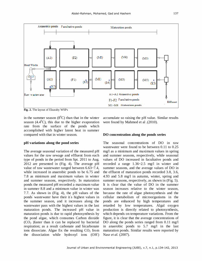
Abdel-Rahman, Mohamed, Gad and Hashem
Journal of Urban and Environmental Engineering (JUEE), v.7, n.1, p.134-142, 2013
137
Fig. 2. The layout of Elzaraby WSPs
in the summer season (80C) than that in the winter season (4.40C), this due to the higher evaporation rate from the surface of the ponds which accomplished with higher latent heat in summer compared with that in winter season.
pH variations along the pond series The average seasonal variation of the measured pH values for the raw sewage and effluent from each type of ponds in the period from Spt. 2011 to Aug. 2012 are presented in (Fig. 4). The average pH value of raw wastewater ranged between 6.63~7.4, while increased in anaerobic ponds to be 6.75 and 7.8 as minimum and maximum values in winter and summer seasons, respectively. In maturation ponds the measured pH recorded a maximum value in summer 8.8 and a minimum value in winter was 7.7. As shown in (Fig. 4), the pH values of the ponds’ wastewater have their it’s highest values in the summer season, and it increases along the wastewater pass with the highest values in the last maturation ponds. The increased pH value in maturation ponds is due to rapid photosynthesis by the pond algae, which consumes Carbon dioxide (CO2 )faster than it can be replaced by bacterial respiration; as a result carbonate and bicarbonate ions dissociate. Algae fix the resulting CO2 from the dissociation while hydroxyl ions (OH-)
accumulate so raising the pH value. Similar results were found by Mahmod et al .(2010).
DO concentration along the ponds series The seasonal concentrations of DO in raw wastewater were found to be between 0.11 to 0.25 mg/l as a minimum and maximum values in spring and summer seasons, respectively, while seasonal values of DO increased in facultative ponds and recorded a range 1.36~2.5 mg/l in winter and summer seasons, and the average values of DO in the effluent of maturation ponds recorded 3.8, 3.6, 4.93 and 5.8 mg/l in autumn, winter, spring and summer seasons, respectively, as shown in (Fig. 5). It is clear that the value of DO in the summer season increases relative to the winter season, because the rate of algae photosynthesis and the cellular metabolism of microorganisms in the ponds are enhanced by high temperatures and retarded by low temperatures. Algal oxygen production is directly related to photosynthesis, which depends on temperature variations. From the figure, it is clear that the average concentrations of DO along the ponds series ranged from 0.11 mg/l in anaerobic ponds to 5.7 mg/l in the last maturation ponds. Similar results were reported by Nasr et al. (2007).
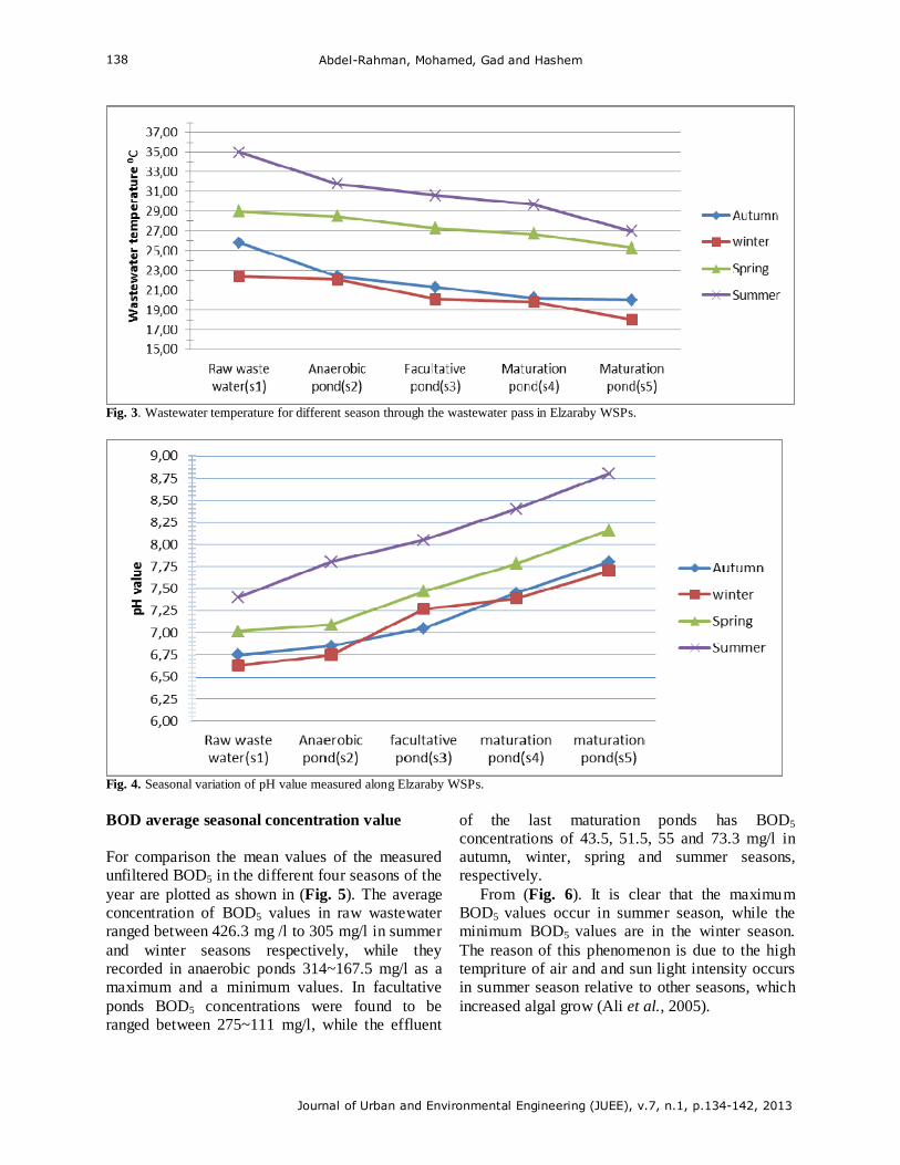
Abdel-Rahman, Mohamed, Gad and Hashem
Journal of Urban and Environmental Engineering (JUEE), v.7, n.1, p.134-142, 2013
138
Fig. 3. Wastewater temperature for different season through the wastewater pass in Elzaraby WSPs.
Fig. 4. Seasonal variation of pH value measured along Elzaraby WSPs.
BOD average seasonal concentration value For comparison the mean values of the measured unfiltered BOD5 in the different four seasons of the year are plotted as shown in (Fig. 5). The average concentration of BOD5 values in raw wastewater ranged between 426.3 mg /l to 305 mg/l in summer and winter seasons respectively, while they recorded in anaerobic ponds 314~167.5 mg/l as a maximum and a minimum values. In facultative ponds BOD5 concentrations were found to be ranged between 275~111 mg/l, while the effluent
of the last maturation ponds has BOD5 concentrations of 43.5, 51.5, 55 and 73.3 mg/l in autumn, winter, spring and summer seasons, respectively.
From (Fig. 6). It is clear that the maximum BOD5 values occur in summer season, while the minimum BOD5 values are in the winter season. The reason of this phenomenon is due to the high tempriture of air and and sun light intensity occurs in summer season relative to other seasons, which increased algal grow (Ali et al., 2005).
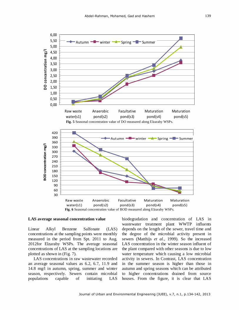
Abdel-Rahman, Mohamed, Gad and Hashem
Journal of Urban and Environmental Engineering (JUEE), v.7, n.1, p.134-142, 2013
139
0,00
0,50
1,00
1,50
2,00
2,50
3,00
3,50
4,00
4,50
5,00
5,50
6,00
Raw waste
water(s1)
Anaerobic
pond(s2)
Facultative
pond(s3)
Maturation
pond(s4)
Maturation
pond(s5)
DO concentration m
g/l
Autumn winter Spring Summer
Fig. 5 Seasonal concentration value of DO measured along Elzaraby WSPs.
30
60
90
120
150
180
210
240
270
300
330
360
390
420
Raw waste
water(s1)
Anaerobic
pond(s2)
Facultative
pond(s3)
Maturation
pond(s4)
Maturation
pond(s5)
BOD concentration mg/l
Autumn winter Spring Summer
Fig. 6 Seasonal concentration value of BOD measured along Elzaraby WSPs.
LAS average seasonal concentration value Linear Alkyl Benzene Salfonate (LAS) concentrations at the sampling points were monthly measured in the period from Spt. 2011 to Aug. 2012for Elzaraby WSPs. The average seasonal concentrations of LAS at the sampling locations are plotted as shown in (Fig. 7).
LAS concentrations in raw wastewater recorded an average seasonal values as 6.2, 6.7, 11.9 and 14.8 mg/l in autumn, spring, summer and winter season, respectively. Sewers contain microbial populations capable of initiating LAS
biodegradation and concentration of LAS in wastewater treatment plant WWTP influents depends on the length of the sewer, travel time and the degree of the microbial activity present in sewers (Matthijs et al., 1999). So the increased LAS concentration in the winter season influent of the plant compared with other seasons is due to low water temperature which causing a low microbial activity in sewers. In Contrast, LAS concentration in the summer season is higher than those in autumn and spring seasons which can be attributed to higher concentrations drained from source houses. From the figure, it is clear that LAS
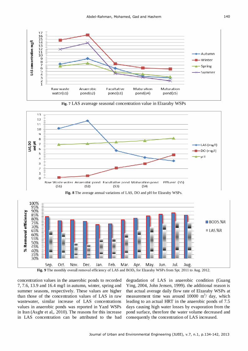
Abdel-Rahman, Mohamed, Gad and Hashem
Journal of Urban and Environmental Engineering (JUEE), v.7, n.1, p.134-142, 2013
140
Fig. 7 LAS avareage seasonal concentration value in Elzaraby WSPs
Fig. 8 The average annual variations of LAS, DO and pH for Elzaraby WSPs.
Fig. 9 The monthly overall removal efficiency of LAS and BOD5 for Elzaraby WSPs from Spt. 2011 to Aug. 2012.
concentration values in the anaerobic ponds to recorded 7, 7.6, 13.9 and 16.4 mg/l in autumn, winter, spring and summer seasons, respectively. These values are higher than those of the concentration values of LAS in raw wastewater, similar increase of LAS concentrations values in anaerobic ponds was reported in Yazd WSPs in Iran (Asghr et al,. 2010). The reasons for this increase in LAS concentration can be attributed to the bad
degradation of LAS in anaerobic condition (Guang Ying, 2004, John Jensen, 1999). the additional reason is that actual average daily flow rate of Elzaraby WSPs at measurement time was around 10000 m3/ day, which leading to an actual HRT in the anaerobic ponds of 7.5 days causing high water losses by evaporation from the pond surface, therefore the water volume decreased and consequently the concentration of LAS increased.
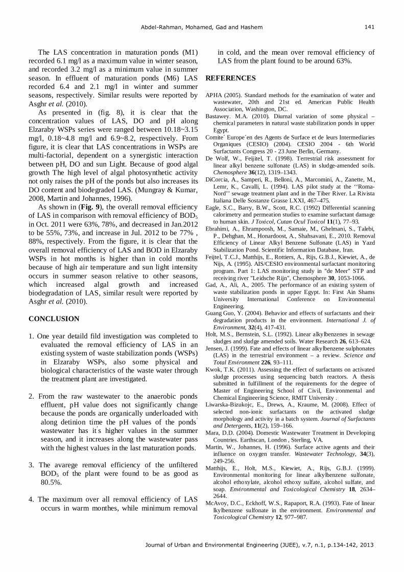
Abdel-Rahman, Mohamed, Gad and Hashem
Journal of Urban and Environmental Engineering (JUEE), v.7, n.1, p.134-142, 2013
141
The LAS concentration in maturation ponds (M1) recorded 6.1 mg/l as a maximum value in winter season, and recorded 3.2 mg/l as a minimum value in summer season. In effluent of maturation ponds (M6) LAS recorded 6.4 and 2.1 mg/l in winter and summer seasons, respectively. Similar results were reported by Asghr et al. (2010).
As presented in (fig. 8), it is clear that the concentration values of LAS, DO and pH along Elzaraby WSPs series were ranged between 10.18~3.15 mg/l, 0.18~4.8 mg/l and 6.9~8.2, respectively. From figure, it is clear that LAS concentrations in WSPs are multi-factorial, dependent on a synergistic interaction between pH, DO and sun Light. Because of good algal growth The high level of algal photosynthetic activity not only raises the pH of the ponds but also increases its DO content and biodegraded LAS. (Mungray & Kumar, 2008, Martin and Johannes, 1996).
As shown in (Fig. 9), the overall removal efficiency of LAS in comparison with removal efficiency of BOD5 in Oct. 2011 were 63%, 78%, and decreased in Jan.2012 to be 55%, 73%, and increase in Jul. 2012 to be 77% , 88%, respectively. From the figure, it is clear that the overall removal efficiency of LAS and BOD in Elzaraby WSPs in hot months is higher than in cold months because of high air temperature and sun light intensity occurs in summer season relative to other seasons, which increased algal growth and increased biodegradation of LAS, similar result were reported by Asghr et al. (2010).
CONCLUSION
1. One year detaild fild investigation was completed to
evaluated the removal efficiency of LAS in an existing system of waste stabilization ponds (WSPs) in Elzaraby WSPs, also some physical and biological characteristics of the waste water through the treatment plant are investigated.
2. From the raw wastewater to the anaerobic ponds
effluent, pH value does not significantly change because the ponds are organically underloaded with along detinion time the pH values of the ponds’
wastewater has it’s higher values in the summer season, and it increases along the wastewater pass with the highest values in the last maturation ponds.
3. The avarege removal efficiency of the unfiltered
BOD5 of the plant were found to be as good as 80.5%.
4. The maximum over all removal efficiency of LAS
occurs in warm monthes, while minimum removal
in cold, and the mean over removal efficiency of LAS from the plant found to be around 63%.
REFERENCES APHA (2005). Standard methods for the examination of water and
wastewater, 20th and 21st ed. American Public Health Association, Washington, DC.
Bastawey. M.A. (2010). Diurnal variation of some physical – chemical parameters in natural waste stabilization ponds in upper Egypt.
Comite´ Europe´en des Agents de Surface et de leurs Intermediaries Organiques (CESIO) (2004). CESIO 2004 - 6th World Surfactants Congress 20 - 23 June Berlin, Germany.
De Wolf, W., Feijitel, T. (1998). Terrestrial risk assessment for linear alkyl benzene sulfonate (LAS) in sludge-amended soils. Chemosphere 36(12), 1319–1343.
DiCorcia, A., Samperi, R., Belloni, A., Marcomini, A., Zanette, M., Lemr, K., Cavalli, L. (1994). LAS pilot study at the ‘‘Roma-Nord’’ sewage treatment plant and in the Tiber River. La Rivista Italiana Delle Sostanze Grasse LXXI, 467–475.
Eagle, S.C., Barry, B.W., Scott, R.C. (1992) Differential scanning calorimetry and permeation studies to examine surfactant damage to human skin. J Toxicol, Cutan Ocul Toxicol 11(1), 77–93.
Ebrahimi, A., Ehrampoosh, M., Samaie, M., Ghelmani, S., Talebi, P., Dehghan, M., Honardoost, A., Shahsavani, E., 2010. Removal Efficiency of Linear Alkyl Benzene Sulfonate (LAS) in Yazd Stabilization Pond. Scientific Information Database, Iran.
Feijtel, T.C.J., Matthijs, E., Rottiers, A., Rijs, G.B.J., Kiewiet, A., de Nijs, A. (1995). AIS/CESIO environmental surfactant monitoring program. Part 1: LAS monitoring study in "de Meer" STP and receiving river "Leidsche Rijn", Chemosphere 30, 1053-1066.
Gad, A., Ali, A., 2005. The performance of an existing system of waste stabilization ponds in upper Egypt. In: First Ain Shams University International Conference on Environmental Engineering.
Guang Guo, Y. (2004). Behavior and effects of surfactants and their degradation products in the environment. International J. of Environment, 32(4), 417-431.
Holt, M.S., Bernstein, S.L. (1992). Linear alkylbenzenes in sewage sludges and sludge amended soils. Water Research 26, 613–624.
Jensen, J. (1999). Fate and effects of linear alkylbenzene sulphonates (LAS) in the terrestrial environment – a review. Science and Total Environment 226, 93–111.
Kwok, T.K. (2011). Assessing the effect of surfactants on activated sludge processes using sequencing batch reactors. A thesis submitted in fulfillment of the requirements for the degree of Master of Engineering School of Civil, Environmental and Chemical Engineering Science, RMIT University .
Liwarska-Bizukojc, E., Drews, A., Kraume, M. (2008). Effect of selected non-ionic surfactants on the activated sludge morphology and activity in a batch system. Journal of Surfactants and Detergents, 11(2), 159–166.
Mara, D.D. (2004). Domestic Wastewater Treatment in Developing Countries. Earthscan, London , Sterling, VA.
Martin, W., Johannes, H. (1996). Surface active agents and their influence on oxygen transfer. Wastewater Technology, 34(3), 249-256.
Matthijs, E., Holt, M.S., Kiewiet, A., Rijs, G.B.J. (1999). Environmental monitoring for linear alkylbenzene sulfonate, alcohol ethoxylate, alcohol ethoxy sulfate, alcohol sulfate, and soap. Environmental and Toxicological Chemistry 18, 2634–2644.
McAvoy, D.C., Eckhoff, W.S., Rapaport, R.A. (1993). Fate of linear lkylbenzene sulfonate in the environment. Environmental and Toxicological Chemistry 12, 977–987.

Abdel-Rahman, Mohamed, Gad and Hashem
Journal of Urban and Environmental Engineering (JUEE), v.7, n.1, p.134-142, 2013
142
Mungray, A.K., Kumar, P. (2008). Occurrence of anionic surfactants in treated sewage: Risk assessment to aquatic environment Journal of Hazardous Materials 160, 362–370.
Nasr. F.A., El-Ashmawy. A., Eltaweel. G., El-Shafai. S.A. (2007). Waste Stabilization Ponds for Wastewater Treatment and Reuse in Egypt. Environmental Sciences Division, Department of Water Pollution Research National Research Center, El-Behoos Street, Dokki, Cairo, Egypt.
Ramadan, H., Ponce, V. (2011). Design and Performance of Waste Stabilization [email protected] Version 081218.
Scott, M.J., Jones. M.N. (2000). The biodegradation of surfactants in the environment. Biochimica et Biophysica Acta 1508 (2000) 235-251.
Trehy, M.L., Gledhil, W.E., Mieure, J.E., Nielsen, A.M., Perkins, H.O., Eckhoff, W.S. (1996). Environmental monitoring for LAS, DATS and their biodegradation intermediate. Environmental Toxicology and chemistry 15(3), 233-240.
Venhuis, S.H., Mehrvar, M. (2004). Health effects, environmental impacts, and photochemical degradation of selected surfactant in water. International Journal of photoenergy 6(2),155-125.
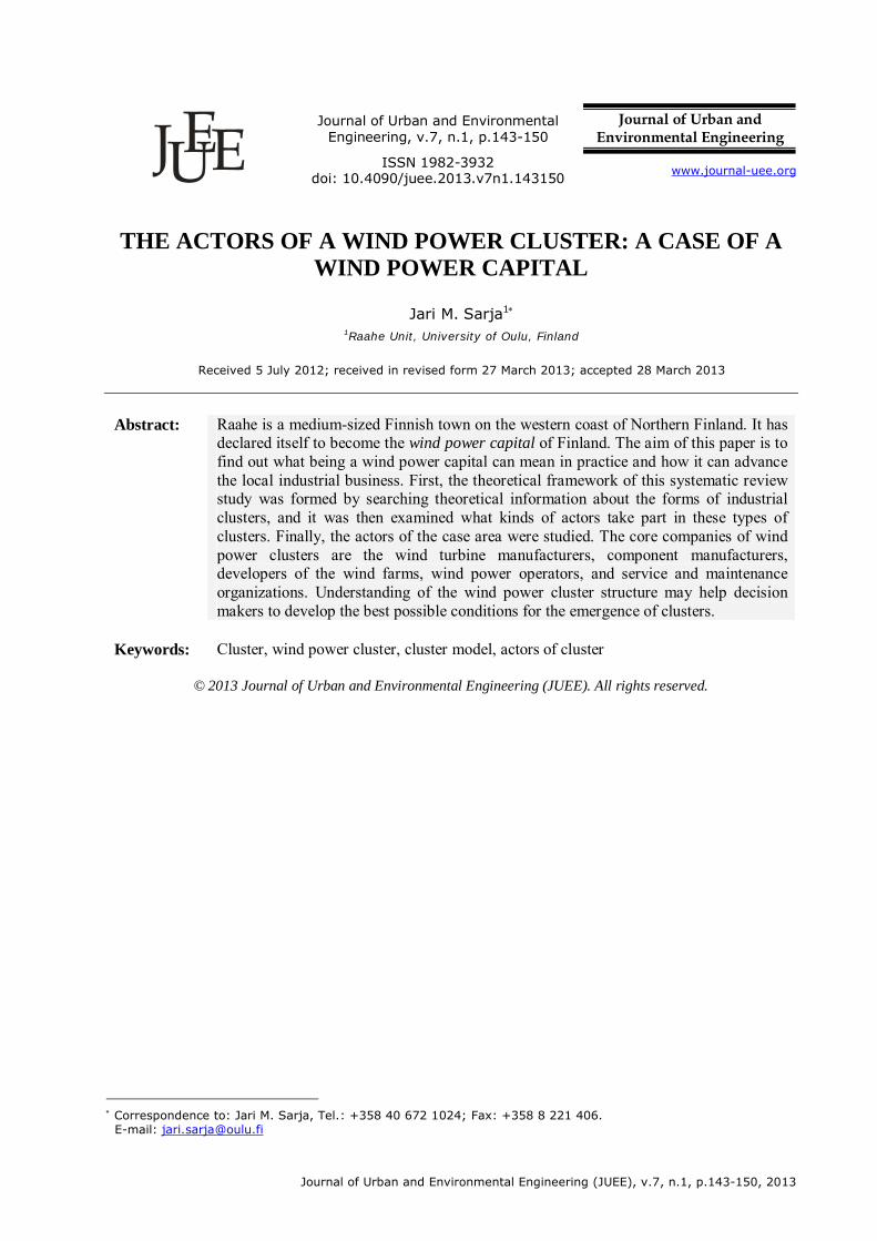
Journal of Urban and Environmental Engineering (JUEE), v.7, n.1, p.143-150, 2013
Journal of Urban and Environmental Engineering, v.7, n.1, p.143-150
Journal of Urban and Environmental Engineering
UEEJ ISSN 1982-3932
doi: 10.4090/juee.2013.v7n1.143150 www.journal-uee.org
THE ACTORS OF A WIND POWER CLUSTER: A CASE OF A WIND POWER CAPITAL
Jari M. Sarja1
1Raahe Unit, University of Oulu, Finland
Received 5 July 2012; received in revised form 27 March 2013; accepted 28 March 2013
Abstract: Raahe is a medium-sized Finnish town on the western coast of Northern Finland. It has
declared itself to become the wind power capital of Finland. The aim of this paper is to find out what being a wind power capital can mean in practice and how it can advance the local industrial business. First, the theoretical framework of this systematic review study was formed by searching theoretical information about the forms of industrial clusters, and it was then examined what kinds of actors take part in these types of clusters. Finally, the actors of the case area were studied. The core companies of wind power clusters are the wind turbine manufacturers, component manufacturers, developers of the wind farms, wind power operators, and service and maintenance organizations. Understanding of the wind power cluster structure may help decision makers to develop the best possible conditions for the emergence of clusters.
Keywords:
Cluster, wind power cluster, cluster model, actors of cluster
© 2013 Journal of Urban and Environmental Engineering (JUEE). All rights reserved.
Correspondence to: Jari M. Sarja, Tel.: +358 40 672 1024; Fax: +358 8 221 406. E-mail: [email protected]
Sarja
Journal of Urban and Environmental Engineering (JUEE), v.7, n.1, p.143-150, 2013
144
INTRODUCTION
The aim of this study was to clarify what kinds of actors take part in wind power clusters and what kinds of possibilities the case area has for the emergence of a wind power cluster. Because there is no specific definition for the concept of wind power cluster, it is first defined on the basis of existing knowledge and combining it using different sources. The actors of a cluster and the possibilities of the case area are then studied.
The case area is the city of Raahe and its sub-region. Raahe is a medium-sized Finnish town on the western coast of Northern Finland (64°41'N, 24°28'E). The location of the case region is shown in Fig. 1. A significant amount, approximately 20 per cent, of Finland's wind power capacity is produced in Raahe and its sub-region. In addition, around twenty new wind farms have been planned for this region (Sarja & Halonen, 2012). Wind farms consist of many wind turbines set in areas favorable for wind power production (e.g. Hossain et al., 2007).
The local media (e.g. Keskinen, 2011; Nousiainen, 2010; Tuikkala, 2010; Veräjänkorva, 2010) has reported about the goal of the city of Raahe to become the wind power capital of Finland. No concrete plans or actions have been commenced yet. The objective of this study is to investigate what being a wind power capital can mean in practice and how it can advance the local industrial business. The wind power capital approach is studied in the framework of cluster theories.
In general, the approach concerns a regional business and know-how center, i.e. a polis or cluster. The polis concepts have been utilized more or less successfully in Northern Finland (e.g. Jauhiainen, 2006). A loose definition of a polis is a know-how center focused on a certain sector of high technology (Multipolis, 2009). A cluster means a business center in which the networked companies strive for competitive advantages with the help of cooperation and common supply chain management (Silen, 2001). From a wider point of view, there are also other actors in clusters in addition to the core companies, namely the suppliers, support businesses, and the public sector including education and research organizations (Porter, 1998).
The wind power cluster seems a promising regional undertaking. There is already heavy industry and its supporting business know-how in the case area, as well as required infrastructure. It can also be said that the case area already has wind power tradition. The wind power capacity of the case area is remarkable in the domestic scale. Besides the conventional energy sources, renewable energy sources including wind power play a vital role in satisfying the energy demand (Hossain et al., 2009).
Fig. 1 Location of the case region.
Moreover, the use of renewable energy sources is
constantly growing, and thus wind power construction is on the increase and there are numerous wind power projects taking place in Finland. Finnish wind power construction is governed by the climate change and energy strategy, which is based on the climate and energy packet initiated by the European Commission in 2008 (Ministry of Employment and the Economy, 2008; European Commission, 2007).
Research and Methods
The research method in this study is systematic review. Systematic review means identifying, evaluating, and interpreting all available research relevant to a particular research question, topic area, or phenomenon of interest (Kitchenham, 2004).
The theoretical material in this study consists of scientific and professional literature on clustering theories. The empirical materials include professional literature, various reports, articles of local media and web sources of the local public sector, open interviews, and for example higher education-level research exercises and theses.
In this review, we have first familiarized with the cluster development theory using especially the diamond model by Porter (1998) and then reviewed the actors of the wind power clusters. Finally, we have analyzed the possibilities of the case area for wind power cluster emergence; what elements and factors already exist and for which elements should the best possible conditions be developed. This model should also clarify the concept of the wind power capital (of Finland). LITERATURE REVIEW
Regional groups of enterprises have been researched as a clustering phenomenon already for a long time. Early researchers, such as Von Thünen (1826), Launhardt (1885), and Weber (1909), explain the benefits of regional networks with savings in transportation costs.
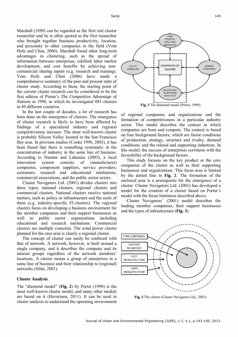
Sarja
Journal of Urban and Environmental Engineering (JUEE), v.7, n.1, p.143-150, 2013
145
Marshall (1890) can be regarded as the first real cluster researcher and he is often quoted as the first researcher who brought together business productivity, location, and proximity to other companies in the field (Vom Hofe and Chen, 2006). Marshall found other long-term advantages in clustering, such as the spread of information between enterprises, (skilled) labor market development, and cost benefits by achieving non-commercial sharing inputs (e.g. research and training). Vom Hofe and Chen (2006) have made a comprehensive summary of the past and present state of cluster study. According to them, the starting point of the current cluster research can be considered to be the first edition of Porter’s The Competitive Advantage of Nations in 1990, in which he investigated 883 clusters in 49 different countries.
In the last couple of decades, a lot of research has been done on the emergence of clusters. The emergence of cluster research is likely to have been affected by findings of a specialized industry and regional competitiveness increase. The most well-known cluster is probably Silicon Valley located in the San Francisco Bay area. In previous studies (Cooke 1998, 2003), it has been found that there is something systematic in the concentration of industry in the same line of business. According to Nummi and Lahenius (2003), a local innovation system consists of (manufacturer) companies, component suppliers, service providers, customers, research and educational institutions, commercial associations, and the public sector actors.
Cluster Navigators Ltd. (2001) divides clusters into three types; national clusters, regional clusters and commercial clusters. National clusters resolve national matters, such as policy or infrastructure and the scale of them (e.g. industry-specific IT-clusters). The regional clusters focus on developing a business environment for the member companies and their support businesses as well as public sector organizations including educational and research institutions. Commercial clusters are multiple consortia. The wind power cluster planned for the case area is clearly a regional cluster.
The concept of cluster can easily be confused with that of network. A network, however, is built around a single company, and it describes the company and its interest groups regardless of the network members’ locations. A cluster means a group of enterprises in a same line of business and their relationship to (regional) networks (Silén, 2001). Cluster Analysis
The “diamond model” (Fig. 2) by Porter (1998) is the most well-known cluster model, and many other models are based on it (Haverinen, 2011). It can be used in cluster analysis to understand the operating environment
Fig. 2 The diamond model (Porter, 1998).
of regional companies and organizations and the formation of competitiveness in a particular industry sector. This model describes the context in which companies are born and compete. The context is based on four background factors, which are factor conditions of production; strategy, structure and rivalry; demand conditions; and the related and supporting industries. In this model, the success of enterprises correlates with the favorability of the background factors.
This study focuses on the key product or the core companies of the cluster as well as their supporting businesses and organizations. This focus area is limited by the dotted line in Fig. 2. The formation of the enclosed area is a prerequisite for the emergence of a cluster. Cluster Navigators Ltd. (2001) has developed a model for the creation of a cluster based on Porter’s model with the focus limitation described above.
Cluster Navigators’ (2001) model describes the leading member companies, their support businesses and the types of infrastructure (Fig. 3).
Fig. 3 The cluster (Cluster Navigators Ltd., 2001).
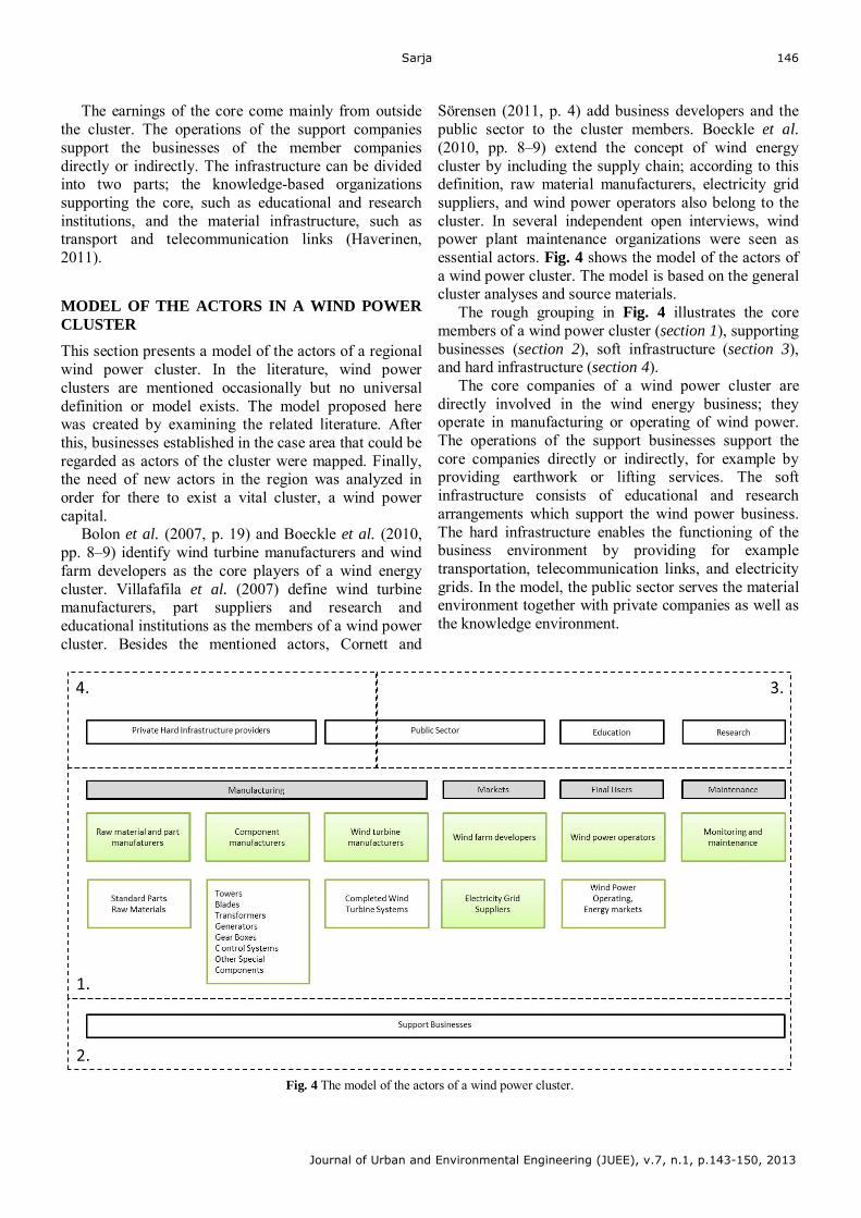
Sarja
Journal of Urban and Environmental Engineering (JUEE), v.7, n.1, p.143-150, 2013
146
The earnings of the core come mainly from outside the cluster. The operations of the support companies support the businesses of the member companies directly or indirectly. The infrastructure can be divided into two parts; the knowledge-based organizations supporting the core, such as educational and research institutions, and the material infrastructure, such as transport and telecommunication links (Haverinen, 2011).
MODEL OF THE ACTORS IN A WIND POWER CLUSTER
This section presents a model of the actors of a regional wind power cluster. In the literature, wind power clusters are mentioned occasionally but no universal definition or model exists. The model proposed here was created by examining the related literature. After this, businesses established in the case area that could be regarded as actors of the cluster were mapped. Finally, the need of new actors in the region was analyzed in order for there to exist a vital cluster, a wind power capital.
Bolon et al. (2007, p. 19) and Boeckle et al. (2010, pp. 8–9) identify wind turbine manufacturers and wind farm developers as the core players of a wind energy cluster. Villafafila et al. (2007) define wind turbine manufacturers, part suppliers and research and educational institutions as the members of a wind power cluster. Besides the mentioned actors, Cornett and
Sörensen (2011, p. 4) add business developers and the public sector to the cluster members. Boeckle et al. (2010, pp. 8–9) extend the concept of wind energy cluster by including the supply chain; according to this definition, raw material manufacturers, electricity grid suppliers, and wind power operators also belong to the cluster. In several independent open interviews, wind power plant maintenance organizations were seen as essential actors. Fig. 4 shows the model of the actors of a wind power cluster. The model is based on the general cluster analyses and source materials.
The rough grouping in Fig. 4 illustrates the core members of a wind power cluster (section 1), supporting businesses (section 2), soft infrastructure (section 3), and hard infrastructure (section 4).
The core companies of a wind power cluster are directly involved in the wind energy business; they operate in manufacturing or operating of wind power. The operations of the support businesses support the core companies directly or indirectly, for example by providing earthwork or lifting services. The soft infrastructure consists of educational and research arrangements which support the wind power business. The hard infrastructure enables the functioning of the business environment by providing for example transportation, telecommunication links, and electricity grids. In the model, the public sector serves the material environment together with private companies as well as the knowledge environment.
Fig. 4 The model of the actors of a wind power cluster.
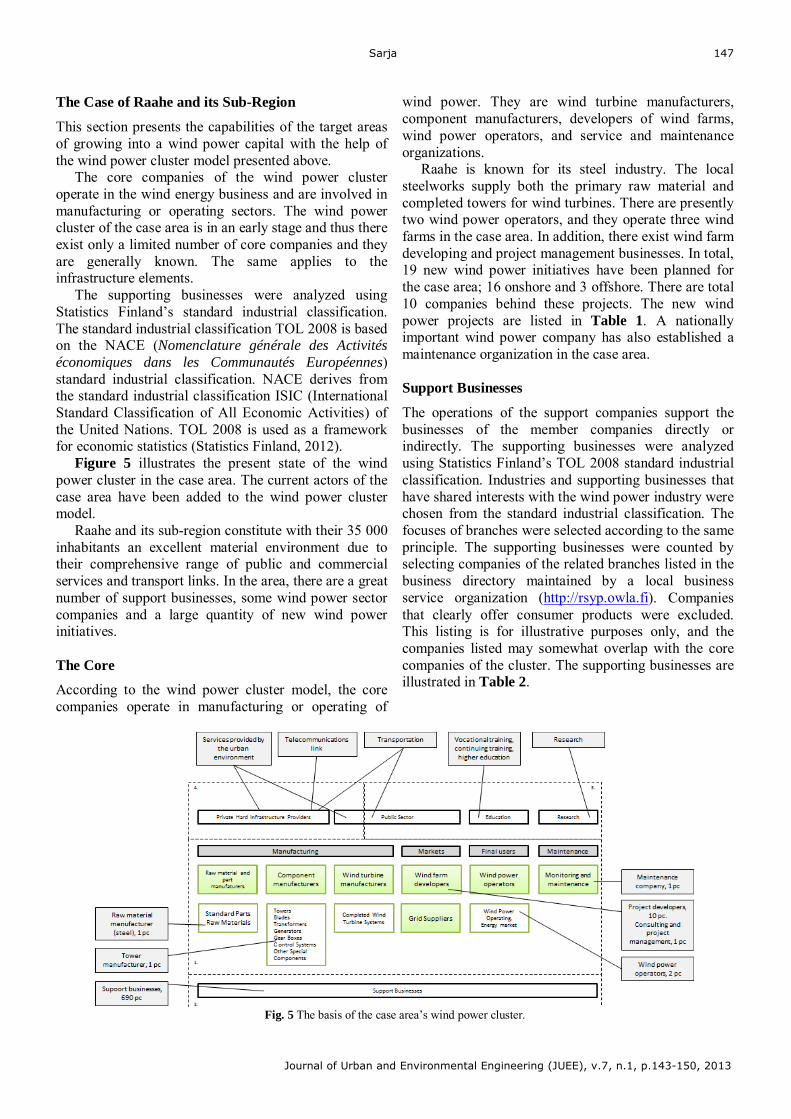
Sarja
Journal of Urban and Environmental Engineering (JUEE), v.7, n.1, p.143-150, 2013
147
The Case of Raahe and its Sub-Region
This section presents the capabilities of the target areas of growing into a wind power capital with the help of the wind power cluster model presented above.
The core companies of the wind power cluster operate in the wind energy business and are involved in manufacturing or operating sectors. The wind power cluster of the case area is in an early stage and thus there exist only a limited number of core companies and they are generally known. The same applies to the infrastructure elements.
The supporting businesses were analyzed using Statistics Finland’s standard industrial classification. The standard industrial classification TOL 2008 is based on the NACE (Nomenclature générale des Activités économiques dans les Communautés Européennes) standard industrial classification. NACE derives from the standard industrial classification ISIC (International Standard Classification of All Economic Activities) of the United Nations. TOL 2008 is used as a framework for economic statistics (Statistics Finland, 2012).
Figure 5 illustrates the present state of the wind power cluster in the case area. The current actors of the case area have been added to the wind power cluster model.
Raahe and its sub-region constitute with their 35 000 inhabitants an excellent material environment due to their comprehensive range of public and commercial services and transport links. In the area, there are a great number of support businesses, some wind power sector companies and a large quantity of new wind power initiatives. The Core
According to the wind power cluster model, the core companies operate in manufacturing or operating of
wind power. They are wind turbine manufacturers, component manufacturers, developers of wind farms, wind power operators, and service and maintenance organizations.
Raahe is known for its steel industry. The local steelworks supply both the primary raw material and completed towers for wind turbines. There are presently two wind power operators, and they operate three wind farms in the case area. In addition, there exist wind farm developing and project management businesses. In total, 19 new wind power initiatives have been planned for the case area; 16 onshore and 3 offshore. There are total 10 companies behind these projects. The new wind power projects are listed in Table 1. A nationally important wind power company has also established a maintenance organization in the case area. Support Businesses
The operations of the support companies support the businesses of the member companies directly or indirectly. The supporting businesses were analyzed using Statistics Finland’s TOL 2008 standard industrial classification. Industries and supporting businesses that have shared interests with the wind power industry were chosen from the standard industrial classification. The focuses of branches were selected according to the same principle. The supporting businesses were counted by selecting companies of the related branches listed in the business directory maintained by a local business service organization (http://rsyp.owla.fi). Companies that clearly offer consumer products were excluded. This listing is for illustrative purposes only, and the companies listed may somewhat overlap with the core companies of the cluster. The supporting businesses are illustrated in Table 2.
Fig. 5 The basis of the case area’s wind power cluster.
Sarja
Journal of Urban and Environmental Engineering (JUEE), v.7, n.1, p.143-150, 2013
148
Table 1. The wind power initiatives in the case area
On the basis of the standard industrial classification, the branches of the selected supporting businesses of the wind power cluster were mining and quarrying (B), manufacturing (C), construction (F), transportation and storage (H), information and communication (J), real estate activities (L), professional, scientific and technical activities (M), and administrative and support service activities (N).
In the case area, companies of each of the selected branches can be found. There is a particularly large number of companies in the manufacturing, construction, transportation and storage, and professional, scientific and technical activities branches. Soft Infrastructure
In this study, the soft infrastructure comprises mainly the educational and research providers of the case area. The soft infrastructure is relatively broad compared to the population. The education available includes education from the basic level to higher education.
Besides the upper secondary school, there exist four vocational schools in the case area. Two of them offer technical programs appropriate for the needs of the cluster. Continuous training is also offered. Higher education is offered by the University of Applied Sciences and the Open University.
The higher educational organizations, the branch office of the University of Oulu, and the national research centre provide research activities.
Table 2. The supporting businesses in the case area
Hard Infrastructure
In this review, the hard infrastructure comprises mainly transportation and telecommunications links. The transportation connections in the case area are excellent in terms of freight traffic, and at least acceptable in terms of passenger traffic. The blind track serving heavy freight comes to the heart of the case area, and it is connected to the main railway network of the country. The nearest railway station for passenger traffic is located on the edge of the case area. The eighth busiest year-round harbor in Finland with more than 700 ships a year is located in the case area. The nearest international airport (Oulu Airport) is located 70 kilometers away from the case area. One of the main highways of the country (Highway 8) cuts through the case area. The telecommunications links are excellent in the entire country (e.g. Grimes, 2003).
In addition, it can be concluded that the city of Raahe with its 23 000 inhabitants and the entire case area including the sub-region with its 35 000 inhabitants with comprehensive commercial and public services compose a functional hard infrastructure for an industrial cluster.
Sarja
Journal of Urban and Environmental Engineering (JUEE), v.7, n.1, p.143-150, 2013
149
CONCLUSIONS
The city of Raahe has announced its plan to become the wind power capital of Finland. The target is logical because the case area is already a significant wind power producer in the national scale, there exist a lot of heavy industrial know-how and networks in the area, and many new wind power initiatives have been planned. New pillars of business life are being actively sought in the traditionally industrial town, and the city can offer a strong operational environment for the new industries.
The study started from the premise that the wind power capital means that the city grows into a strong wind power cluster. It can be said that there is already a small-scale wind power cluster in the case area with a few wind energy business companies. However, the existing companies operate as relatively independent actors, and the cluster includes no very noteworthy supply chains.
Because there is no universal definition or model of a wind power cluster in the literature, we have proposed a model of the actors of a wind power cluster by examining the related literature. We propose that the actors of a wind power cluster are wind turbine manufacturers, raw material and component manufacturers, wind farm developers, wind power operators, grid suppliers, service organizations, research and educational institutions, public sector actors, support businesses, and (both private and public) infrastructure providers.
We compared the core companies, support businesses, infrastructure, and public services of the case area with the wind power cluster model. We found out that there are a few wind power-related companies in the case area, and they provide a good basis for the emergence of a cluster. After sifting, almost 700 support businesses were found in the case area. There is education available from the basic level to higher education, and research support exists, so it can be concluded that soft infrastructure is acceptable regarding the size of the case area. It can be said that the hard infrastructure in the case area is excellent because of existing heavy industry and working freight traffic solutions including shipping, rail traffic, and road transport.
Therefore, the conditions for the emergence of a nationally significant wind power cluster are good. We think the next step would be to market the area and develop the best possible conditions for the core companies of the wind energy business outside the case area. The missing core companies are especially wind turbine (see Fig. 5) and part manufacturers, but a larger number of other core companies would also profit the area. In addition, it should be ensured that the education
and research available are able to serve the needs of this kind of cluster also in future.
The practical relevance of this study is to help the decision makers of the case area to piece together the present state of the wind power capital and to see what kinds of actors should be drawn in. This study may also offer new aspects for the wider local energy cluster strategy, which is a part of the business strategy of the case area. The theoretical contribution of this study is the definition of a universal model of a wind power cluster in a general level. It can be used in other studies in the field and focused and updated by taking into account local circumstances. Acknowledgement The research material for this work was collected in “Green Technology” project supported in part by the European Regional Development Fund (ERDF) of the European Union. REFERENCES
Bolon, E., Commons, M., Des Rosiers, F., Caso de los Cobos, P.G. & Kukrika, N. (2007) The Spanish wind power cluster. [online] Final report Microeconomics of competitiveness, Harvard Business School, Harvard University. Available from: http://www.isc.hbs.edu/pdf/Student_Projects/Spain_WindPowerCluster_2007.pdf (Accessed 22 March 2012).
Cluster Navigators Ltd. (2001) Cluster Building: A toolkit. [online] Available in: www.vaxtarsamningur.is/Files/Skra_0023777.pdf.
Cooke, P. (1998) Introduction: Origins of the Concept. [online] Regional Innovation Systems, 1998. Available at SSRN: http://ssrn.com/abstract=1497770
Cooke, P. (2003) Economic globalization and its future challenges for regional development. International Journal in Technology Management 26 (2), 401–420.
Cornett, A.P. & Sörensen, N.K. (2011) Regional economic aspects of the Danish Windmill Cluster: The case of the emerging off shore wind energy cluster on the west coast of Jutland”, Proceedings of the 14th Uddevalla Symposium, June 16–18, 2011, Bergamo, Italy.
European Commission (2007) Combating climate change – The EU leads the way. [online] Belgium. Available from: http://ec.europa.eu/publications/booklets/move/70/en.pdf (Accessed 28 February 2012).
Grimes, S. (2003) The digital economy challenge facing peripheral rural areas. Progress in Human Geography 27(2), 174–193.
Haverinen, K. (2011) Edellytyksiä Kajaanin datakeskus-klusterille, MS thesis, University of Oulu, Oulu, Finland (in Finnish).
Hossain, A., Iqbal, A.K.M.P., Rahman, A., Arifin, M. & Mazian, M. (2007) Design and development of a 1/3 scale vertical axis wind turbine for electrical power generation. J. Urban Environm. Engin. 2(2), 1–5.
Hossain, A., Rahman, A., Rahman, M., Hasan, S.K. & Hossen, J. (2009) Prediction of power generation of small scale vertical axis wind turbine using fuzzy logic. J. Urban Environm. Engin. 3(2), 43–51.
Jauhiainen, J. (2006) Multipolis: High-technology network in Northern Finland. Europ. Plan. Studies 14(10), 1407–1428.
Keskinen, S. (2011) Olisiko tyvenen paikka? Raahen Seutu 14 June 2011 (In Finnish).
Sarja
Journal of Urban and Environmental Engineering (JUEE), v.7, n.1, p.143-150, 2013
150
Kitchenham, B. (2004) Procedures for performing systematic reviews. Keele University Technical Report.
Launhardt, W. (1885) Mathematische Begründung der Wolkwirtschaftslehre. B.G. Teubner, Leipzig (in German).
Marshall, A. (1890) Principles of Economics. Macmillan, London. Multipolis (2009) Welcome to Multipolis. Available from:
http://www.multipolis.com/index.php?189 (Accessed 4 March 2012).
Nousiainen, T. (2010) Raahe sai tukikohdan. Raahen Seutu 1 December 2010 (in Finnish).
Nummi, J. & Lahenius, K. (2004) Medical devices innovation networks in Oulu Region as local innovation system. Frontiers of e-Business Research 2003. Feb 2003. Conference proceedings, September 24–25, 2003, Tampere, Finland.
Porter, M. E. (1998) The competitive advantage of nations. MacMillan, London.
Sarja, J. & Halonen, V. (2012) A case study of a wind turbine sourcing: manufacturer selection criteria. Proceedings of the annual Electrical Power and Energy Conference. Oct 2012. pp: 266-271.
Sileń, T. (2001). Laatu, brändi ja kilpailukyky. WSOY, Helsinki (in Finnish).
Statistics Finland (2012) Standard Industrial Classification TOL 2008. Available in: http://www.stat.fi/meta/luokitukset/toimiala/0012008/index_en.html. (Accessed 22 May 2012).
Tuikkala, K. (2010) Tuulivoimapääkaupungiksi. Raahen Seutu 23 November 2010 (in Finnish).
Ministry of Employment and the Economy (2008) Climate Change and Energy Strategy 2008. Government Report to Parliament 6 November 2008. Available from: http://www.tem.fi/index.phtml?l=en&s=2658 (Accessed 28 February 2012).
Veräjänkorva, A. (2010) Jari Sillanpää sijoittaa Raahen tuulivoimaan. Yle Oulu. Available from: http://yle.fi/alueet/oulu/2010/11/jari_sillanpaa_sijoittaa_raahen_tuulivoimaan_2162218.html (Accessed 6 March 2012).
Villafafila, R., Sumper, A., Suwannarat, A., Bak-Jensen, B., Ramirez, R., Gomis, O. & Sudria, A. (2007) On wind power integration into electrical power system: Spain vs. Denmark. Poster session presented at International Conference on Renewable Energies and Power Quality, ICREPQ'07, Sevilla, Spain.
vom Hofe, R. & Chen, K. (2006) Whither or not industrial cluster: conclusions or confusions? The Industrial Geographer 4(1), 2–28.
Von Thünen, J.H. (1826) Der isolierte Staat in Beziehung auf Landwirtschaft und Nationalökonomie. Perthes, Hamburg.
Weber, A. (1909) Über den Standort der Industrien. J.C.B Mohr, Tübingen, Germany.
Journal of Urban and Environmental Engineering (JUEE), v.7, n.1, p.151-156, 2013
Journal of Urban and Environmental Engineering, v.7, n.1, p.151-156
Journal of Urban and Environmental Engineering
UEEJ ISSN 1982-3932
doi: 10.4090/juee.2013.v7n1.151156 www.journal-uee.org
FLOW PHYSICS OF 3-BLADED STRAIGHT CHORD H-DARRIEUS WIND TURBINE
Rajat Gupta¹ and Agnimitra Biswas²
¹Director, National Institute of Technology Srinagar, Srinagar, Jammu & Kashmir, India
²Assistent Professor, National Institute of Technology Silchar, Silchar, Assam, India
Received 30 March 2013; received in revised form 9 May 2013; accepted 30 May 2013
Abstract: Steady-state two-dimensional Computational Fluid Dynamics (CFD) simulations were
performed using Fluent 6.0 software to analyze the flow physics of 3-bladed straight chord H-Darrieus wind turbine having blade twist of 300 for 10% of its chord at the trailing ends. The flow was simulated using finite volume method coupled with moving mesh technique to solve mass and momentum conservation equations. The standard k-ε turbulence model with enhanced wall condition was used. Second-order upwind discretization scheme was adopted for pressure-velocity coupling of the flow. Flow physics of the turbine was analyzed with the help of pressure and velocity contours. It was found that velocity magnitude decreases from upstream to downstream side across the turbine, which will cause overall lift for the turbine. Further, blade twist at the trailing ends creates circulations that interact with the blades in a direction opposite to the direction of rotation of the turbine which would enhance power production for the three bladed turbine.
Keywords:
H-Darrieus turbine, straight chord blade, CFD analysis, contours
© 2013 Journal of Urban and Environmental Engineering (JUEE). All rights reserved.
Correspondence to: Agnimitra Biswas, Tel.: Fax: +091-3842-233797, Phone: +0091-3842-248308. E-mail: [email protected]
Gupta and Biswas
Journal of Urban and Environmental Engineering (JUEE), v.7, n.1, p.151-156, 2013
152
INTRODUCTION
The straight-bladed Vertical Axis Wind Turbine (VAWT), H-Darrieus turbine, is an invention included in the Darrieus patent (Darrieus, 1931). The H-Darrieus turbine, also known as H-rotor after its inventor, is a lift type device, which has two to three blades designed as airfoils. The blades are attached vertically to the central shaft through support arms. The support to the vertical axis helps the turbine maintain its shape. The H-Darrieus turbine is normally placed on the top of a tower in order to reach higher winds. Moreover, the H-Darrieus turbine is the most suitable turbine in extreme wind conditions, like wind gusts, cyclone, and its efficiency could be as high as Horizontal Axis Wind Turbine (HAWT) when placed on rooftops (Mertens, 2003).
Guy wires are generally used to support the shaft of eggbeater Darrieus turbine since it gives a stiffer, more robust construction. However, guy wires are optional for H-Darrieus turbine, which is an advantage. It is self-regulating in all wind speeds reaching its optimal rotational speed shortly after its cut-in wind speed (Islam et al., 2005). The blades of H-Darrieus turbine are much easier to manufacture than the blades of a HAWT or of an eggbeater Darrieus turbine. Light weight, highly flexible turbines are usually two-bladed turbines. Visual aesthetics and lower noise are the reasons for using three-bladed designs. Tangtonsakulwong & Chitsomboon (2006) did Computational Fluid Dynamics (CFD) simulation of wind flow over an untwisted three-bladed H-Darrieus turbine of NACA 0015 blade profile by using 3D unstructured-mesh finite volume method together with the sliding mesh technique to solve mass and momentum conservation equations. The maximum power coefficient of 0.20 was obtained at a tip speed ratio of 2.9. Jiang et al. (2007) developed 2D CFD models to study the effects of number of blades and tip speed ratio on the performance of multi-bladed H-Darrieus turbines. However, the highest power coefficient of their turbine was about 19%. Howell et al. (2010) studied the performances of two-bladed and three-bladed H-Darrieus turbines through wind tunnel experiments and also through CFD analyses. The two-bladed turbine had a higher peak power coefficient of 0.25 compared to about 0.22 for the three-bladed turbine.
Twist blades could be a good field of research since such blades have the potential to be superior to the untwisted blades. Tip geometry can locally modify the angle of attack and the inflow dynamic pressure and hence can improve performance of the turbine. But experimental or computational works in this direction are very few. Keeping this in view, in this paper, an
attempt was made to study the performance of a three-bladed H-Darrieus turbine having blade twist of 300 for 10% of its chord at the trailing ends. Two dimensional simulations were run using Fluent 6.0 CFD software. Pressure and velocity contours were analyzed and performance of the present turbine was predicted from the analysis. Model Design The height of the turbine was 20cm, and the chord length of the blades was 5 cm. An angular twist of 300 was provided at the tips of the chords for 10% of chord length from the trailing end. The turbine is shown in the Fig.1 respectively. The blades were supported on bolts 5mm in diameter & 12 cm in length. The central shaft of the turbines was 1.5 cm in diameter and about 25 cm in length. By changing the overall turbine diameter but keeping the height constant, ten numbers of H/D ratios were obtained. The central shaft, base and the supports were made from mild steel, and the blades were made from lightweight aluminium. Ball bearings were used to support the shaft of the turbines at the base. The base was 7cm wide and 2.4 cm thick.
A Figura 1 dee vir aqui dentro desta caixa de texto para ficar na 1a. página.
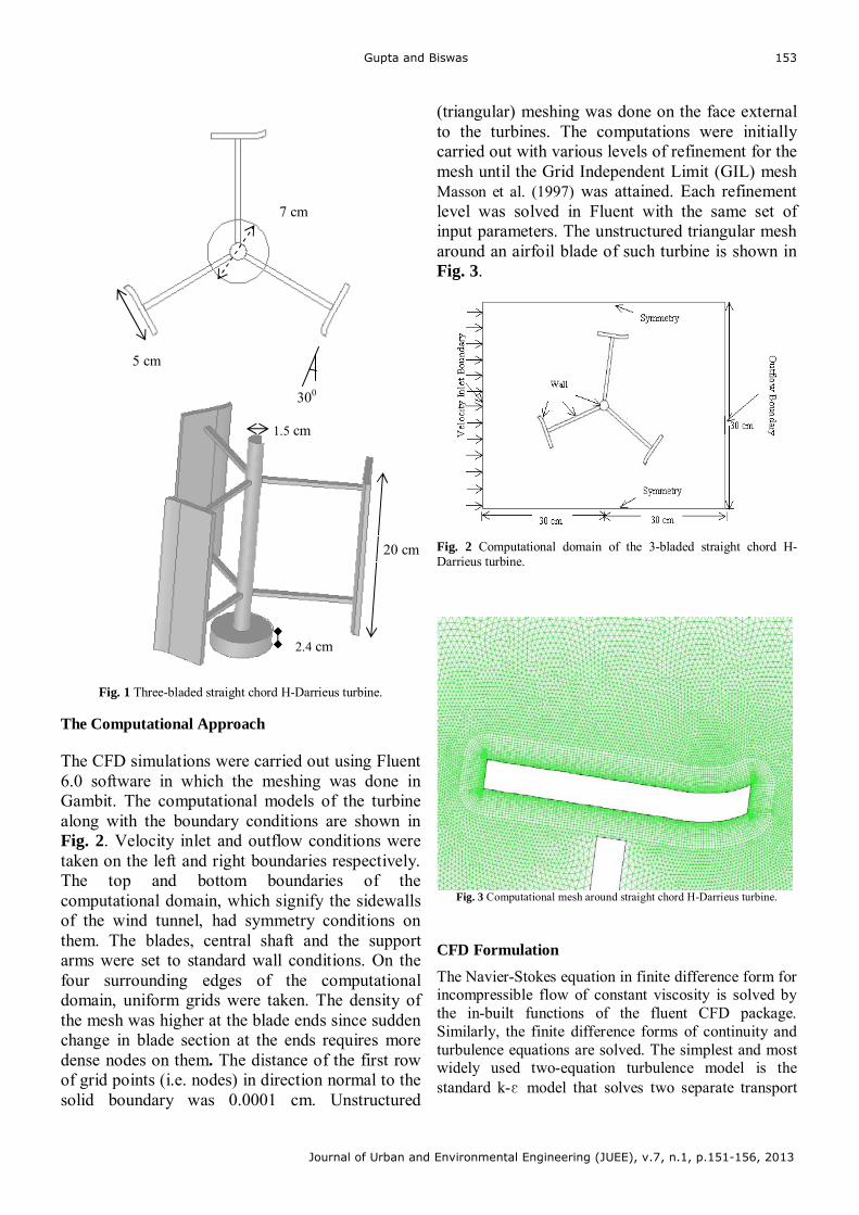
Gupta and Biswas
Journal of Urban and Environmental Engineering (JUEE), v.7, n.1, p.151-156, 2013
153
Fig. 1 Three-bladed straight chord H-Darrieus turbine.
The Computational Approach The CFD simulations were carried out using Fluent 6.0 software in which the meshing was done in Gambit. The computational models of the turbine along with the boundary conditions are shown in Fig. 2. Velocity inlet and outflow conditions were taken on the left and right boundaries respectively. The top and bottom boundaries of the computational domain, which signify the sidewalls of the wind tunnel, had symmetry conditions on them. The blades, central shaft and the support arms were set to standard wall conditions. On the four surrounding edges of the computational domain, uniform grids were taken. The density of the mesh was higher at the blade ends since sudden change in blade section at the ends requires more dense nodes on them. The distance of the first row of grid points (i.e. nodes) in direction normal to the solid boundary was 0.0001 cm. Unstructured
(triangular) meshing was done on the face external to the turbines. The computations were initially carried out with various levels of refinement for the mesh until the Grid Independent Limit (GIL) mesh Masson et al. (1997) was attained. Each refinement level was solved in Fluent with the same set of input parameters. The unstructured triangular mesh around an airfoil blade of such turbine is shown in Fig. 3.
Fig. 2 Computational domain of the 3-bladed straight chord H-Darrieus turbine.
Fig. 3 Computational mesh around straight chord H-Darrieus turbine.
CFD Formulation
The Navier-Stokes equation in finite difference form for incompressible flow of constant viscosity is solved by the in-built functions of the fluent CFD package. Similarly, the finite difference forms of continuity and turbulence equations are solved. The simplest and most widely used two-equation turbulence model is the standard k-ε model that solves two separate transport
300
5 cm
20 cm
1.5 cm
7 cm
2.4 cm
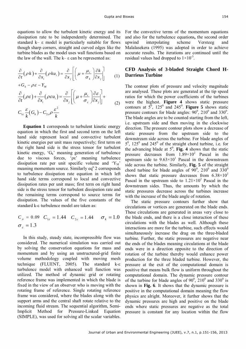
Gupta and Biswas
Journal of Urban and Environmental Engineering (JUEE), v.7, n.1, p.151-156, 2013
154
equations to allow the turbulent kinetic energy and its dissipation rate to be independently determined. The standard k– ε model is particularly suitable for flows though sharp corners, straight and curved edges like the turbine blades as the model uses wall functions based on the law of the wall. The k– ε can be represented as:
ti
i j k j
k M
kk ku
t x x x
G Y
(1)
2
1 2
ti
i j j
k
ut x x x
C G Ck k
(2)
Equation 1 corresponds to turbulent kinetic energy
equation in which the first and second term on the left hand side represent local and convective turbulent kinetic energies per unit mass respectively; first term on the right hand side is the stress tensor for turbulent kinetic energy, ‘Gk’ meaning generation of turbulence due to viscous forces, ‘ρε’ meaning turbulence dissipation rate per unit specific volume and ‘YM’ meaning momentum source. Similarly eqn 2 corresponds to turbulence dissipation rate equation in which left hand side terms correspond to local and convective dissipation rates per unit mass; first term on right hand side is the stress tensor for turbulent dissipation rate and the remaining terms correspond to source terms for dissipation. The values of the five constants of the standard k- turbulence model are taken as:
09.0C 44.11 C 44.12 C 0.1k 3.1
In this study, steady state, incompressible flow was
considered. The numerical simulation was carried out by solving the conservation equations for mass and momentum and by using an unstructured-grid finite volume methodology coupled with moving mesh technique (FLUENT, 2005). The standard k- turbulence model with enhanced wall function was utilized. The method of dynamic grid or rotating reference frame was implemented in which the blade is fixed in the view of an observer who is moving with the rotating frame of reference. Single rotating reference frame was considered, where the blades along with the support arms and the central shaft rotate relative to the incoming fluid stream. The sequential algorithm, Semi-Implicit Method for Pressure-Linked Equation (SIMPLE), was used for solving all the scalar variables.
For the convective terms of the momentum equations and also for the turbulence equations, the second order upwind interpolating scheme Versteeg and Malalasekera (1995) was adopted in order to achieve accurate results. The iterations are continued until the residual values had dropped to 1×10⁻³. CFD Analysis of 3-bladed Straight Chord H-Darrieus Turbine The contour plots of pressure and velocity magnitude are analysed. These plots are generated at the tip speed ratios for which the power coefficients of the turbines were the highest. Figure 4 shows static pressure contours at 50, 1250 and 2450. Figure 5 shows static pressure contours for blade angles: 900, 2100 and 3300. The blade angles are to be counted starting from the left, i.e. upstream side and then moving in the clockwise direction. The pressure contour plots show a decrease of static pressure from the upstream side to the downstream side across the turbine. For blade angles of 50, 1250 and 2450 of the straight chord turbine, i.e. for the advancing blade at 50, Fig. 4 shows that the static pressure decreases from 1.89×10² Pascal in the upstream side to 9.63×101 Pascal in the downstream side across the turbine. Similarly, Fig. 5 of the straight chord turbine for blade angles of 900, 2100 and 3300 shows that static pressure decreases from 6.38×10² Pascal in the upstream side to 1.21×10² Pascal in the downstream sides. Thus, the amounts by which the static pressures decrease across the turbines increase with the increase of the blade angle of rotation.
The static pressure contours further show that circulations or vortices are generated on the blade ends. These circulations are generated in areas very close to the blade ends, and there is a close interaction of these circulations with the blades as well. Although these interactions are more for the turbine, such effects would simultaneously increase the drag on the three-bladed turbine. Further, the static pressures are negative near the ends of the blades meaning circulations at the blade ends were in a direction opposite to the direction of rotation of the turbine thereby would enhance power production for the three bladed turbine. However, the pressure at the exit of the computational domain is positive that means bulk flow is uniform throughout the computational domain. The dynamic pressure contour of the turbine for blade angles of 900, 2100 and 3300 is shown in Fig. 6. It shows that the dynamic pressure is positive in the computational domain meaning the flow physics are alright. Moreover, it further shows that the dynamic pressures are high and positive on the blade ends where static pressures are negative as the total pressure is constant for any location within the flow
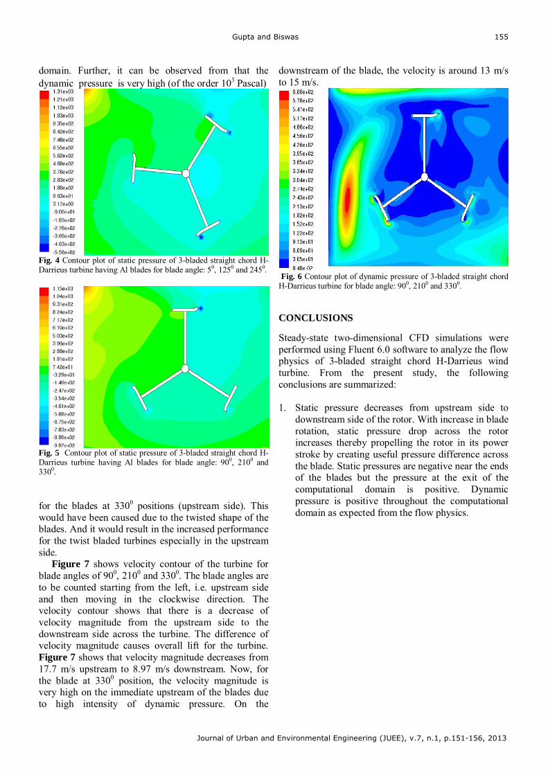
Gupta and Biswas
Journal of Urban and Environmental Engineering (JUEE), v.7, n.1, p.151-156, 2013
155
domain. Further, it can be observed from that the
dynamic pressure is very high (of the order 103 Pascal)
Fig. 4 Contour plot of static pressure of 3-bladed straight chord H-Darrieus turbine having Al blades for blade angle: 50, 1250 and 2450.
Fig. 5 Contour plot of static pressure of 3-bladed straight chord H-Darrieus turbine having Al blades for blade angle: 900, 2100 and 3300. for the blades at 3300 positions (upstream side). This would have been caused due to the twisted shape of the blades. And it would result in the increased performance for the twist bladed turbines especially in the upstream side.
Figure 7 shows velocity contour of the turbine for blade angles of 900, 2100 and 3300. The blade angles are to be counted starting from the left, i.e. upstream side and then moving in the clockwise direction. The velocity contour shows that there is a decrease of velocity magnitude from the upstream side to the downstream side across the turbine. The difference of velocity magnitude causes overall lift for the turbine. Figure 7 shows that velocity magnitude decreases from 17.7 m/s upstream to 8.97 m/s downstream. Now, for the blade at 3300 position, the velocity magnitude is very high on the immediate upstream of the blades due to high intensity of dynamic pressure. On the
downstream of the blade, the velocity is around 13 m/s to 15 m/s.
Fig. 6 Contour plot of dynamic pressure of 3-bladed straight chord H-Darrieus turbine for blade angle: 900, 2100 and 3300.
CONCLUSIONS
Steady-state two-dimensional CFD simulations were performed using Fluent 6.0 software to analyze the flow physics of 3-bladed straight chord H-Darrieus wind turbine. From the present study, the following conclusions are summarized: 1. Static pressure decreases from upstream side to
downstream side of the rotor. With increase in blade rotation, static pressure drop across the rotor increases thereby propelling the rotor in its power stroke by creating useful pressure difference across the blade. Static pressures are negative near the ends of the blades but the pressure at the exit of the computational domain is positive. Dynamic pressure is positive throughout the computational domain as expected from the flow physics.
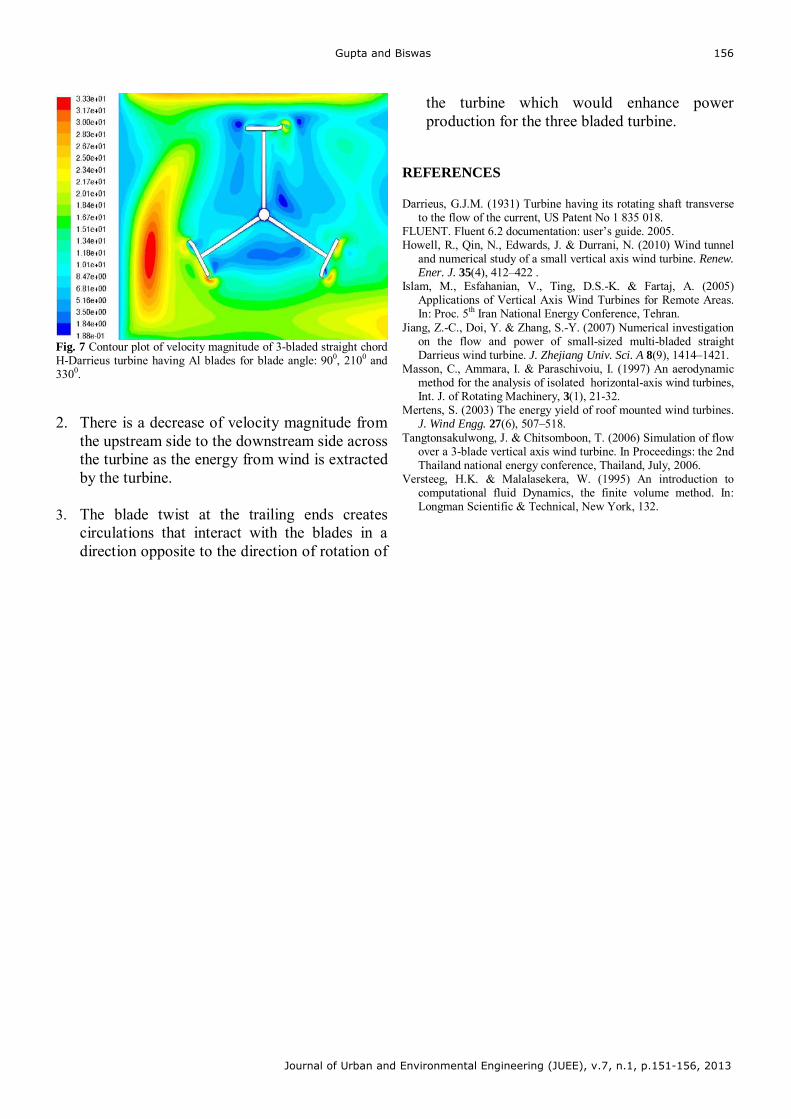
Gupta and Biswas
Journal of Urban and Environmental Engineering (JUEE), v.7, n.1, p.151-156, 2013
156
Fig. 7 Contour plot of velocity magnitude of 3-bladed straight chord H-Darrieus turbine having Al blades for blade angle: 900, 2100 and 3300.
2. There is a decrease of velocity magnitude from
the upstream side to the downstream side across the turbine as the energy from wind is extracted by the turbine.
3. The blade twist at the trailing ends creates
circulations that interact with the blades in a direction opposite to the direction of rotation of
the turbine which would enhance power production for the three bladed turbine.
REFERENCES
Darrieus, G.J.M. (1931) Turbine having its rotating shaft transverse to the flow of the current, US Patent No 1 835 018.
FLUENT. Fluent 6.2 documentation: user’s guide. 2005. Howell, R., Qin, N., Edwards, J. & Durrani, N. (2010) Wind tunnel
and numerical study of a small vertical axis wind turbine. Renew. Ener. J. 35(4), 412–422 .
Islam, M., Esfahanian, V., Ting, D.S.-K. & Fartaj, A. (2005) Applications of Vertical Axis Wind Turbines for Remote Areas. In: Proc. 5th Iran National Energy Conference, Tehran.
Jiang, Z.-C., Doi, Y. & Zhang, S.-Y. (2007) Numerical investigation on the flow and power of small-sized multi-bladed straight Darrieus wind turbine. J. Zhejiang Univ. Sci. A 8(9), 1414–1421.
Masson, C., Ammara, I. & Paraschivoiu, I. (1997) An aerodynamic method for the analysis of isolated horizontal-axis wind turbines, Int. J. of Rotating Machinery, 3(1), 21-32.
Mertens, S. (2003) The energy yield of roof mounted wind turbines. J. Wind Engg. 27(6), 507–518.
Tangtonsakulwong, J. & Chitsomboon, T. (2006) Simulation of flow over a 3-blade vertical axis wind turbine. In Proceedings: the 2nd Thailand national energy conference, Thailand, July, 2006.
Versteeg, H.K. & Malalasekera, W. (1995) An introduction to computational fluid Dynamics, the finite volume method. In: Longman Scientific & Technical, New York, 132.
Journal of Urban and Environmental Engineering, v.7, n.1, p.157-163
Journal of Urban and Environmental Engineering, v.7, n.1, p.157-163
Journal of Urban and Environmental Engineering
UEEJ ISSN 1982-3932
doi: 10.4090/juee.2013.v7n1.157163 www.journal-uee.org
ANAEROBIC EFFLUENT POST-TREATMENT APPLYING PHOTOLYTIC REACTOR PRIOR TO AGRICULTURAL USE IN
BRAZILIAN SEMIARID REGION
José Tavares de Sousa¹, Geralda Gilvânea Cavalcante Lima¹, Wilton Silva Lopes¹, Eclésio Cavalcante Santo² and José Lima de Oliveira Júnior³
1 Department of Sanitary and Environmental Engineering of the State University of Paraíba ² Master in Science and Environmental Technology by the State University of Paraíba
³ Department of Environmental Engineering of the Federal Institute of Ceará
Received 21 August 2012; received in revised form 19 January 2013; accepted 24 June 2013
Abstract: This work applied a Compact System consisting of a Reactor Up flow Sludge Blanket (UASB) in conjunction with s Submerged Anaerobic Filter containing polyurethane cubes as support media, followed by a Solar Photolytic Reactor. The compact anaerobic system produced a clarified effluent with low concentration of organic matter, especially dissolved (20 mg.VSS/L), and free of helminthes eggs. These low concentrations of suspended solids facilitated photolytic disinfection process producing a good quality final effluent, of which 90% of the samples were thoroughly disinfected, while the other fraction showed concentration of Thermotolerant Coliform (TTC) at or below 100 CFU/100 mL and high concentrations of nutrients (48 mg.NH4
+-N/L and 6.4 mg.PO4-3-
P/L) enabling the use of irrigation for productive purposes. Another advantages of the compact anaerobic treatment consisted of low sludge production, and relatively simple operation without energy consumption. These advantages results in a significant reduction in operational costs of sewage treatment, and, indeed, an outlet for developing countries in tropical climate.
Keywords:
Anaerobic system; post-treatment; photolytic reactor; removal of pathogenic organisms.
Correspondence to: José Tavares de Sousa. E-mail: [email protected]
Sousa, Lima, Lopes, Santo and Oliveira Júnior
Journal of Urban and Environmental Engineering, v.7, n.1, p.157-163
158
INTRODUCTION
Access to sanitation can be understood as an indicator of a society development state. The universalization and improvement in quality of sanitation services can be considered as one of the biggest challenges of the country, requiring an investment of 178 billion dollars over the next 20 years (UNDP, 2004).
Treating sewage properly, with secondary treatment followed by a tertiary one, like filtration and disinfection for production of sanitary quality effluent required by the World Health Organization can be too expensive and difficult to implement, especially in developing countries. From a practical point of view searching new technologies or adapt existing ones is a desirable goal in order to deal more economical and environmentally with the large amount of sewage generated by urban and suburban populations.
The application of anaerobic treatment systems is of great importance, as they allow the removal of organic matter without the need for energy consumption required in aerobic processes. Other advantages include: low production of solid methane formation (which can be recovered) and disposing of equipment for aeration.
Among the major technological advances in the application of anaerobic digestion processes in wastewater treatment is the development of the UASB, especially for application in tropical and subtropical countries, where the temperature stays above 20oC. Their efficiency is related to the flow direction and configuration (presence of three phase separator), which allows longer cell retention, while providing an adequate stirring and mixing between the affluent and the sludge blanket Foresti et al., 2006).
The UASB reactor consists of a low cost alternative in the treatment of domestic sewage, providing a removal of about 70% of BOD5 and low hydraulic retention time (HRT) from 5 to 8 hours (Além Sobrinho; Kato, 1999). However, the disposal of effluents into water bodies requires post-treatment to reduce or eliminate pathogens and reduce the concentration of nutrients like nitrogen and phosphorus.
When the destination is the reuse of wastewater in agriculture, necessarily, there is demand for removal or inactivation of pathogenic organisms like viruses, bacteria, protozoa and helminthes, which create serious public health problems affecting workers in plantations as well as consumers of these cultures (Sousa et al., 2009).
The microorganisms present in domestic wastewater are usually vulnerable to heat and ultraviolet radiation. Once the sun is a free available source of heat and radiation it can be used as a source of UV disinfection processes. So, one can use photolysis process via UV for effluent disinfection, especially in semiarid region of Northeast Brazil, where the sunshine lasts an average of 2,800 h/year (Sousa et al., 2005).
In this context, this study propose was to apply an anaerobic treatment of domestic sewage using system composed by a compact anaerobic UASB combined with anaerobic filter and effluent post-treatment in Solar Photolytic Reactor. It is understood as a low-cost technology able to produce effluent of good sanitary quality, low organic load and considerable concentration of nutrients.
MATERIAL AND METHODS
The experiment took place at the station of Biological Treatment of Sewage (EXTRABES) located in an area belonging both to the Company of Water and Sewers of Paraíba state (CAGEPA) and the State University of Paraíba in Campina Grande, Paraíba State, with altitude of 550 m.
The municipal wastewater used during the experiment was captured by a submersible pump installed in an inspection well from the CAGEPA’s sewer Interceptor Pipe. The sewage fed by gravity, through plastic hoses of 20 mm in diameter, a box of 100 liters, where there was peristaltic metering pump with preset flow feeding system.
The experimental system of wastewater treatment illustrated in Fig. 1 was composed of two units. The
Fig. 1 Schematic of anaerobic reactor followed by Solar Photocatalitic Reactor.
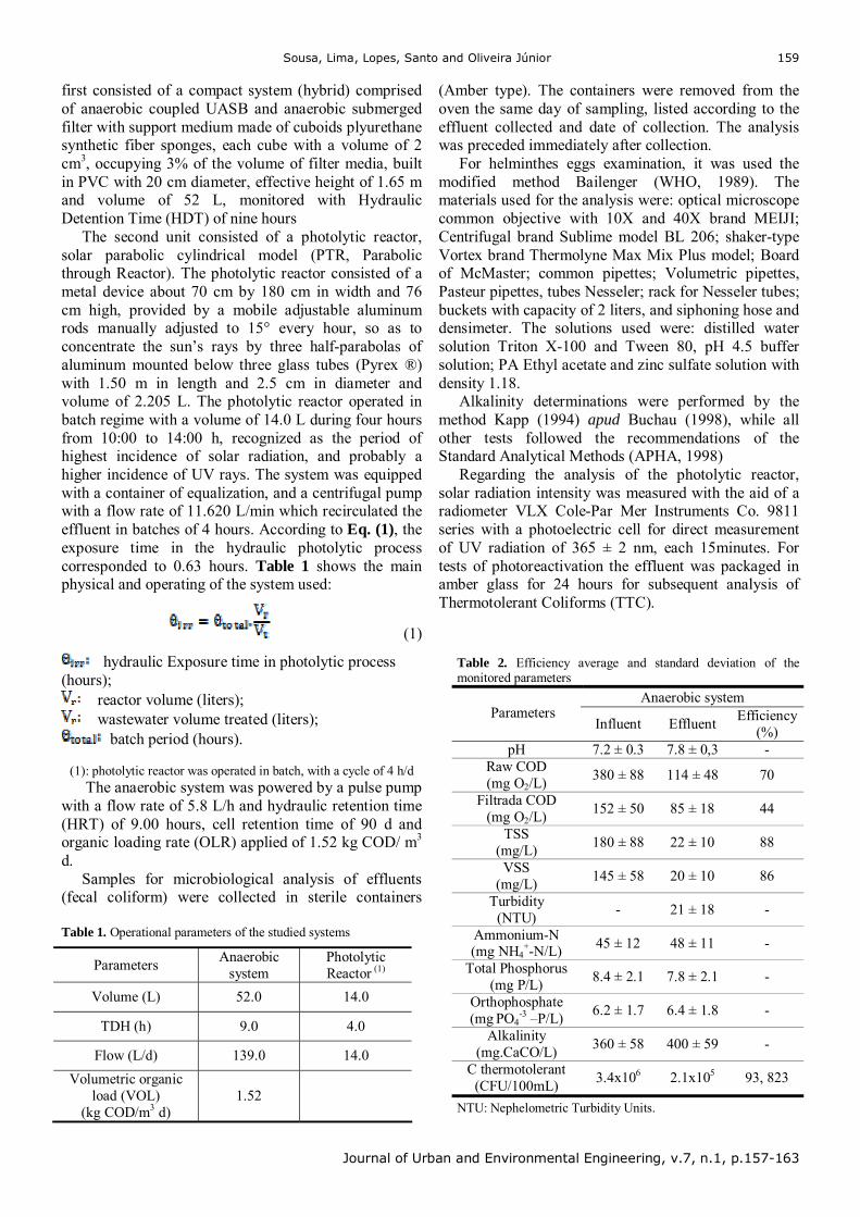
Sousa, Lima, Lopes, Santo and Oliveira Júnior
Journal of Urban and Environmental Engineering, v.7, n.1, p.157-163
159
first consisted of a compact system (hybrid) comprised of anaerobic coupled UASB and anaerobic submerged filter with support medium made of cuboids plyurethane synthetic fiber sponges, each cube with a volume of 2 cm3, occupying 3% of the volume of filter media, built in PVC with 20 cm diameter, effective height of 1.65 m and volume of 52 L, monitored with Hydraulic Detention Time (HDT) of nine hours
The second unit consisted of a photolytic reactor, solar parabolic cylindrical model (PTR, Parabolic through Reactor). The photolytic reactor consisted of a metal device about 70 cm by 180 cm in width and 76 cm high, provided by a mobile adjustable aluminum rods manually adjusted to 15° every hour, so as to concentrate the sun’s rays by three half-parabolas of aluminum mounted below three glass tubes (Pyrex ®) with 1.50 m in length and 2.5 cm in diameter and volume of 2.205 L. The photolytic reactor operated in batch regime with a volume of 14.0 L during four hours from 10:00 to 14:00 h, recognized as the period of highest incidence of solar radiation, and probably a higher incidence of UV rays. The system was equipped with a container of equalization, and a centrifugal pump with a flow rate of 11.620 L/min which recirculated the effluent in batches of 4 hours. According to Eq. (1), the exposure time in the hydraulic photolytic process corresponded to 0.63 hours. Table 1 shows the main physical and operating of the system used:
(1)
hydraulic Exposure time in photolytic process (hours);
reactor volume (liters); wastewater volume treated (liters);
batch period (hours).
(1): photolytic reactor was operated in batch, with a cycle of 4 h/d The anaerobic system was powered by a pulse pump
with a flow rate of 5.8 L/h and hydraulic retention time (HRT) of 9.00 hours, cell retention time of 90 d and organic loading rate (OLR) applied of 1.52 kg COD/ m3 d.
Samples for microbiological analysis of effluents (fecal coliform) were collected in sterile containers
(Amber type). The containers were removed from the oven the same day of sampling, listed according to the effluent collected and date of collection. The analysis was preceded immediately after collection.
For helminthes eggs examination, it was used the modified method Bailenger (WHO, 1989). The materials used for the analysis were: optical microscope common objective with 10X and 40X brand MEIJI; Centrifugal brand Sublime model BL 206; shaker-type Vortex brand Thermolyne Max Mix Plus model; Board of McMaster; common pipettes; Volumetric pipettes, Pasteur pipettes, tubes Nesseler; rack for Nesseler tubes; buckets with capacity of 2 liters, and siphoning hose and densimeter. The solutions used were: distilled water solution Triton X-100 and Tween 80, pH 4.5 buffer solution; PA Ethyl acetate and zinc sulfate solution with density 1.18.
Alkalinity determinations were performed by the method Kapp (1994) apud Buchau (1998), while all other tests followed the recommendations of the Standard Analytical Methods (APHA, 1998)
Regarding the analysis of the photolytic reactor, solar radiation intensity was measured with the aid of a radiometer VLX Cole-Par Mer Instruments Co. 9811 series with a photoelectric cell for direct measurement of UV radiation of 365 ± 2 nm, each 15minutes. For tests of photoreactivation the effluent was packaged in amber glass for 24 hours for subsequent analysis of Thermotolerant Coliforms (TTC).
Table 1. Operational parameters of the studied systems
Parameters Anaerobic
system Photolytic Reactor (1)
Volume (L) 52.0 14.0
TDH (h) 9.0 4.0
Flow (L/d) 139.0 14.0
Volumetric organic load (VOL)
(kg COD/m3 d) 1.52
Table 2. Efficiency average and standard deviation of the monitored parameters
Anaerobic system Parameters
Influent Effluent Efficiency
(%) pH 7.2 ± 0.3 7.8 ± 0,3 -
Raw COD (mg O2/L)
380 ± 88 114 ± 48 70
Filtrada COD (mg O2/L)
152 ± 50 85 ± 18 44
TSS (mg/L)
180 ± 88 22 ± 10 88
VSS (mg/L)
145 ± 58 20 ± 10 86
Turbidity (NTU)
- 21 ± 18 -
Ammonium-N (mg NH4
+-N/L) 45 ± 12 48 ± 11 -
Total Phosphorus (mg P/L)
8.4 ± 2.1 7.8 ± 2.1 -
Orthophosphate (mg PO4
-3 –P/L) 6.2 ± 1.7 6.4 ± 1.8 -
Alkalinity (mg.CaCO/L)
360 ± 58 400 ± 59 -
C thermotolerant (CFU/100mL)
3.4x10⁶ 2.1x10⁵ 93, 823
NTU: Nephelometric Turbidity Units.
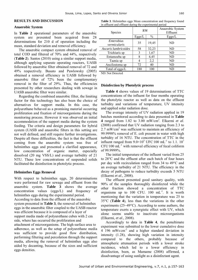
Sousa, Lima, Lopes, Santo and Oliveira Júnior
Journal of Urban and Environmental Engineering, v.7, n.1, p.157-163
160
RESULTS AND DISCUSSION
Anaerobic System
In Table 2 operational parameters of the anaerobic system are presented been acquired from 28 determinations for 210 d of operation including the mean, standard deviation and removal efficiency.
The anaerobic compact system obtained removal of total COD and filtered of 70% and 44%, respectively (Table 2). Santos (2010) using a similar support media, although applying separate operating reactors, UASB followed by anaerobic filter obtained removal of 72 and 49% respectively. Busato and Pawlowsky (2005) obtained a removal efficiency in UASB followed by anaerobic filter of 72% been the complementary removal in the filter of 29%. Thus, the efficiencies presented by other researchers dealing with sewage in UASB anaerobic filter were similar.
Regarding the combined anaerobic filter, the limiting factor for this technology has also been the choice of alternatives for support media. In this case, the polyurethane behaved as a promising material occurring proliferation and fixation of microorganisms during the monitoring process. However it was observed an initial accommodation of the support media during the system feeding. The criteria and design parameters for hybrid system (UASB and anaerobic filters in this setting are not well defined, and still require further investigations. Despite all these difficulties, the fact is that the effluent coming from the anaerobic system was free of helminthes eggs and presented a clarified appearance, low concentration of organic matter, especially dissolved (20 mg VSS/L) and average turbidity of 21 NTU. These low concentrations of suspended solids facilitated the disinfection in photolytic process. Helminthes Eggs Removal
With respect to helminthes eggs, 20 determinations were performed for raw sewage and effluent from the anaerobic system. Table 3 shows the average concentration values (eggs/L) and frequency of helminthes eggs during the experimental period. According to data from the effluent of the anaerobic system presented in Table 3, the removal of helminthes eggs in the anaerobic filter coupled to the UASB reactor was efficient because it is composed of a layer of support media made of polyurethane cubes with 2 cm side, where has occurred the proliferation and attachment of microorganisms. The high surface area to adherence, as well as the setup of polyurethane media was sufficient to provide good flow distribution, performing filtering and percolation through the support media, allowing the removal of helminthes eggs also aided by decanting, because of the sizes and sufficient eggs densities.
Disinfection by Photolytic process
Table 4 shows values of 19 determinations of TTC concentrations of the influent for four months operating the photolytic reactor as well as data on the effluent turbidity and variations of temperature, UV intensity and applied solar radiation dose.
The average intensity of UV radiation applied in 19 batches monitored according to data presented in Table 4 ranged from 1.82 to 3.00 mW/cm2. Elkarmi et al. (2008) confirmed that UV radiation ranging from 2.3 to 2.7 mW/cm2 was sufficient to maintain an efficiency of 99.9998% removal of E. coli present in water with high turbidity of 16 NTU. The concentration of TTC in the influent ranged from 9.0×10⁵ UFC.100 mL-1 to 1.1. 107
CFU.100 mL-1 with removal efficiency of fecal coliform of 99.9999%.
The initial temperature of the influent varied from 25 to 28°C and the effluent after each batch of four hours per day with recirculation ranged from 34 to 49°C and an average turbidity of 21 NTU. The efficiency in the decay of pathogens to reduce turbidity exceeds 5 NTU (Elkarmi et al., 2008).
The effluent presented good sanitary quality, with 90% of the samples thoroughly disinfected while the other fraction showed a concentration of TTC organisms up to 100 CFU. 100 mL-1. It is worth mentioning that the variation in temperature was 25 to 35°C (Table 4), less than the variations in the other experiments (2549°C). According to some authors, the temperature exerts a synergistic effect with UV, which alone seems unable to inactivate microorganisms (Elkarmi, et al., 2008).
Accordingly to data in Table 4, the penultimate experiment was submitted to the lower cumulative dose 4 196 mWs.cm-2 and a higher standard deviation in intensity (1.28), showing high variation in intensity compared to the others, probably because of atmospheric attenuation periods with a lower stroke incidence, which led to a lower efficiency in disinfection, been, as Mamame (2008) affirmed, a disadvantage of using sunlight as a disinfectant agent.
Table 3. Helminthes eggs Mean concentration and frequency found in affluent and effluent during the experimental period
RW Anaerobic System
Effluent Species Eggs/L % Eggs/L
Enterobius vermicularis 35 19,45 ND
Ascaris lumbricoides 58 32,23 ND Trichiuris sp 3 1,67 ND
Entamoeba sp 8 4,45 ND Taenia sp 4 2,2 ND
Ancilostoma sp 72 40 ND Total of eggs/L 180 100 ND
ND: Not Detected
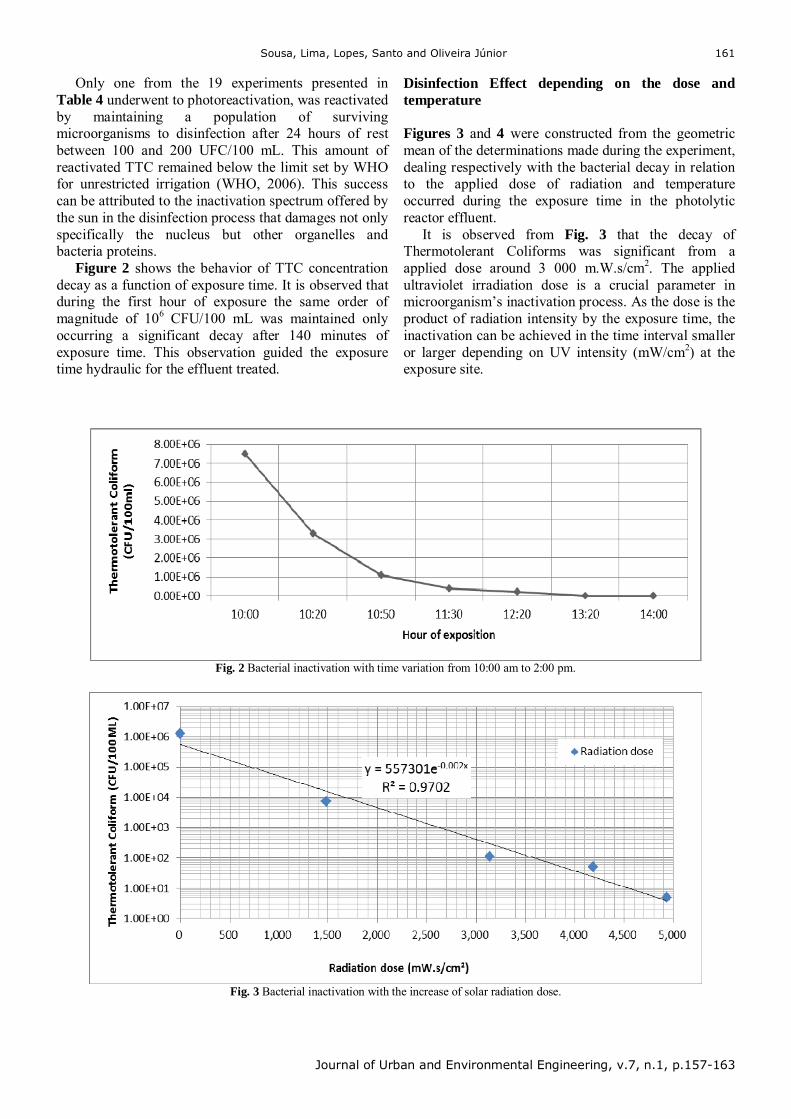
Sousa, Lima, Lopes, Santo and Oliveira Júnior
Journal of Urban and Environmental Engineering, v.7, n.1, p.157-163
161
Only one from the 19 experiments presented in Table 4 underwent to photoreactivation, was reactivated by maintaining a population of surviving microorganisms to disinfection after 24 hours of rest between 100 and 200 UFC/100 mL. This amount of reactivated TTC remained below the limit set by WHO for unrestricted irrigation (WHO, 2006). This success can be attributed to the inactivation spectrum offered by the sun in the disinfection process that damages not only specifically the nucleus but other organelles and bacteria proteins.
Figure 2 shows the behavior of TTC concentration decay as a function of exposure time. It is observed that during the first hour of exposure the same order of magnitude of 106 CFU/100 mL was maintained only occurring a significant decay after 140 minutes of exposure time. This observation guided the exposure time hydraulic for the effluent treated.
Disinfection Effect depending on the dose and temperature Figures 3 and 4 were constructed from the geometric mean of the determinations made during the experiment, dealing respectively with the bacterial decay in relation to the applied dose of radiation and temperature occurred during the exposure time in the photolytic reactor effluent.
It is observed from Fig. 3 that the decay of Thermotolerant Coliforms was significant from a applied dose around 3 000 m.W.s/cm2. The applied ultraviolet irradiation dose is a crucial parameter in microorganism’s inactivation process. As the dose is the product of radiation intensity by the exposure time, the inactivation can be achieved in the time interval smaller or larger depending on UV intensity (mW/cm2) at the exposure site.
Fig. 2 Bacterial inactivation with time variation from 10:00 am to 2:00 pm.
Fig. 3 Bacterial inactivation with the increase of solar radiation dose.
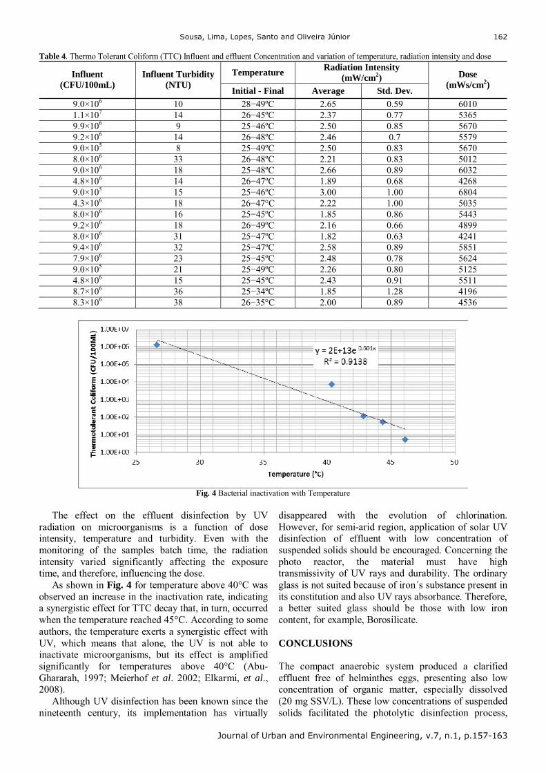
Sousa, Lima, Lopes, Santo and Oliveira Júnior
Journal of Urban and Environmental Engineering, v.7, n.1, p.157-163
162
Table 4. Thermo Tolerant Coliform (TTC) Influent and effluent Concentration and variation of temperature, radiation intensity and dose
Temperature Radiation Intensity
(mW/cm2) Influent (CFU/100mL)
Influent Turbidity (NTU)
Initial - Final Average Std. Dev.
Dose (mWs/cm2)
9.0×10⁶ 10 28−49ºC 2.65 0.59 6010 1.1×10⁷ 14 26−45ºC 2.37 0.77 5365 9.9×10⁶ 9 25−46ºC 2.50 0.85 5670 9.2×10⁶ 14 26−48ºC 2.46 0.7 5579 9.0×10⁵ 8 25−49ºC 2.50 0.83 5670 8.0×10⁶ 33 26−48ºC 2.21 0.83 5012 9.0×10⁶ 18 25−48ºC 2.66 0.89 6032 4.8×10⁶ 14 26−47ºC 1.89 0.68 4268 9.0×10⁵ 15 25−46ºC 3.00 1.00 6804 4.3×10⁶ 18 26−47°C 2.22 1.00 5035 8.0×10⁶ 16 25−45ºC 1.85 0.86 5443 9.2×10⁶ 18 26−49ºC 2.16 0.66 4899 8.0×10⁶ 31 25−47ºC 1.82 0.63 4241 9.4×10⁶ 32 25−47ºC 2.58 0.89 5851 7.9×10⁶ 23 25−45ºC 2.48 0.78 5624 9.0×10⁵ 21 25−49ºC 2.26 0.80 5125 4.8×10⁶ 15 25−45ºC 2.43 0.91 5511 8.7×10⁶ 36 25−34ºC 1.85 1.28 4196 8.3×10⁶ 38 26−35°C 2.00 0.89 4536
Fig. 4 Bacterial inactivation with Temperature
The effect on the effluent disinfection by UV
radiation on microorganisms is a function of dose intensity, temperature and turbidity. Even with the monitoring of the samples batch time, the radiation intensity varied significantly affecting the exposure time, and therefore, influencing the dose.
As shown in Fig. 4 for temperature above 40°C was observed an increase in the inactivation rate, indicating a synergistic effect for TTC decay that, in turn, occurred when the temperature reached 45°C. According to some authors, the temperature exerts a synergistic effect with UV, which means that alone, the UV is not able to inactivate microorganisms, but its effect is amplified significantly for temperatures above 40°C (Abu-Ghararah, 1997; Meierhof et al. 2002; Elkarmi, et al., 2008).
Although UV disinfection has been known since the nineteenth century, its implementation has virtually
disappeared with the evolution of chlorination. However, for semi-arid region, application of solar UV disinfection of effluent with low concentration of suspended solids should be encouraged. Concerning the photo reactor, the material must have high transmissivity of UV rays and durability. The ordinary glass is not suited because of iron´s substance present in its constitution and also UV rays absorbance. Therefore, a better suited glass should be those with low iron content, for example, Borosilicate. CONCLUSIONS The compact anaerobic system produced a clarified effluent free of helminthes eggs, presenting also low concentration of organic matter, especially dissolved (20 mg SSV/L). These low concentrations of suspended solids facilitated the photolytic disinfection process,
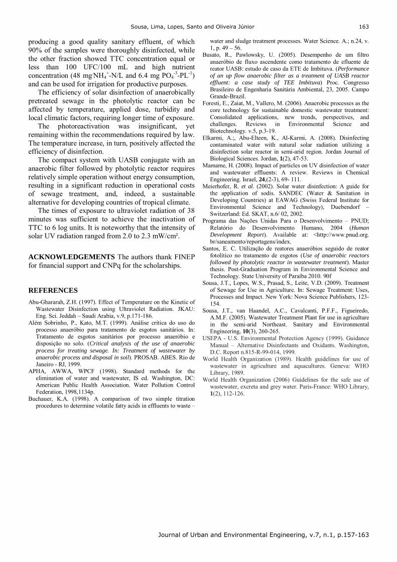
Sousa, Lima, Lopes, Santo and Oliveira Júnior
Journal of Urban and Environmental Engineering, v.7, n.1, p.157-163
163
producing a good quality sanitary effluent, of which 90% of the samples were thoroughly disinfected, while the other fraction showed TTC concentration equal or less than 100 UFC/100 mL and high nutrient concentration (48 mg.NH4
+-N/L and 6.4 mg PO4-3-PL-1)
and can be used for irrigation for productive purposes. The efficiency of solar disinfection of anaerobically
pretreated sewage in the photolytic reactor can be affected by temperature, applied dose, turbidity and local climatic factors, requiring longer time of exposure.
The photoreactivation was insignificant, yet remaining within the recommendations required by law. The temperature increase, in turn, positively affected the efficiency of disinfection.
The compact system with UASB conjugate with an anaerobic filter followed by photolytic reactor requires relatively simple operation without energy consumption, resulting in a significant reduction in operational costs of sewage treatment, and, indeed, a sustainable alternative for developing countries of tropical climate.
The times of exposure to ultraviolet radiation of 38 minutes was sufficient to achieve the inactivation of TTC to 6 log units. It is noteworthy that the intensity of solar UV radiation ranged from 2.0 to 2.3 mW/cm².
ACKNOWLEDGEMENTS The authors thank FINEP for financial support and CNPq for the scholarships.
REFERENCES
Abu-Ghararah, Z.H. (1997). Effect of Temperature on the Kinetic of Wastewater Disinfection using Ultraviolet Radiation. JKAU: Eng. Sci. Jeddah – Saudi Arabia, v.9, p.171-186.
Além Sobrinho, P., Kato, M.T. (1999). Análise crítica do uso do processo anaeróbio para tratamento de esgotos sanitários. In: Tratamento de esgotos sanitários por processo anaeróbio e disposição no solo. (Critical analysis of the use of anaerobic process for treating sewage. In: Treatment of wastewater by anaerobic process and disposal in soil). PROSAB. ABES. Rio de Janeiro - RJ, 1999.
APHA, AWWA, WPCF (1998). Standard methods for the elimination of water and wastewater, IS ed. Washington, DC: American Public Health Association. Water Pollution Control Federation, 1998,1134p.
Buchauer, K.A. (1998). A comparison of two simple titration procedures to determine volatile fatty acids in effluents to waste –
water and sludge treatment processes. Water Science. A.; n.24, v. 1, p. 49 – 56.
Busato, R., Pawlowsky, U. (2005). Desempenho de um filtro anaeróbio de fluxo ascendente como tratamento de efluente de reator UASB: estudo de caso da ETE de Imbituva. (Performance of an up flow anaerobic filter as a treatment of UASB reactor effluent: a case study of TEE Imbituva) Proc. Congresso Brasileiro de Engenharia Sanitária Ambiental, 23, 2005. Campo Grande-Brazil.
Foresti, E., Zaiat, M., Vallero, M. (2006). Anaerobic processes as the core technology for sustainable domestic wastewater treatment: Consolidated applications, new trends, perspectives, and challenges. Reviews in Environmental Science and Biotechnology. v.5, p.3-19.
Elkarmi, A.;, Abu-Elteen, K., Al-Karmi, A. (2008). Disinfecting contaminated water with natural solar radiation utilizing a disinfection solar reactor in semi-arid region. Jordan Journal of Biological Sciences. Jordan, 1(2), 47-53.
Mamame, H. (2008). Impact of particles on UV disinfection of water and wastewater effluents: A review. Reviews in Chemical Engineering. Israel, 24,(2-3), 69- 111.
Meierhofer, R. et al. (2002). Solar water disinfection: A guide for the application of sodis. SANDEC (Water & Sanitation in Developing Countries) at EAWAG (Swiss Federal Institute for Environmental Science and Technology), Duebendorf – Switzerland: Ed. SKAT, n.6/ 02, 2002.
Programa das Nações Unidas Para o Desenvolvimento – PNUD; Relatório do Desenvolvimento Humano, 2004 (Human Development Report). Available at: <http://www.pnud.org. br/saneamento/reportagens/index.
Santos, E. C. Utilização de reatores anaeróbios seguido de reator fotolítico no tratamento de esgotos (Use of anaerobic reactors followed by photolytic reactor in wastewater treatment). Master thesis. Post-Graduation Program in Environmental Science and Technology. State University of Paraíba 2010. 90f
Sousa, J.T., Lopes, W.S., Prasad, S., Leite, V.D. (2009). Treatment of Sewage for Use in Agriculture. In: Sewage Treatment: Uses, Processes and Impact. New York: Nova Science Publishers, 123-154.
Sousa, J.T., van Haandel, A.C., Cavalcanti, P.F.F., Figueiredo, A.M.F. (2005). Wastewater Treatment Plant for use in agriculture in the semi-arid Northeast. Sanitary and Environmental Engineering, 10(3), 260-265.
USEPA - U.S. Environmental Protection Agency (1999). Guidance Manual – Alternative Disinfectants and Oxidants. Washington, D.C. Report n.815-R-99-014, 1999.
World Health Organization (1989). Health guidelines for use of wastewater in agriculture and aquacultures. Geneva: WHO Library, 1989.
World Health Organization (2006) Guidelines for the safe use of wastewater, excreta and grey water. Paris-France: WHO Library, 1(2), 112-126.
Journal of Urban and Environmental Engineering (JUEE), v.7, n.1, p.164-175, 2013
Journal of Urban and Environmental Engineering, v.7, n.1, p.164-175
Journal of Urban and Environmental Engineering
UEEJ ISSN 1982-3932
doi: 10.4090/juee.2013.v7n1.164175 www.journal-uee.org
RETROFITTING OF REINFORCED CONCRETE BEAMS USING FIBRE REINFORCED POLYMER (FRP)
COMPOSITES – A REVIEW
Namasivayam Aravind1, Amiya K. Samanta2, D. K. Singha Roy2 and Joseph V. Thanikal1
1Department of Built and Natural Environment, Caledonian College of Engineering, Oman 2Department of Civil Engineering, National Institute of Technology Durgapur, India
Received 6 February 2013; received in revised form 31 May 2013; accepted 06 June 2013
Abstract: Rehabilitation and strengthening of old structures using advanced materials is a
contemporary research in the field of Structural Engineering. During past two decades, much research has been carried out on shear and flexural strengthening of reinforced concrete beams using different types of fibre reinforced polymers and adhesives. Strengthening of old structures is necessary to obtain an expected life span. Life span of Reinforced Concrete (RC) structures may be reduced due to many reasons, such as deterioration of concrete and development of surface cracks due to ingress of chemical agents, improper design and unexpected external lateral loads such as wind or seismic forces acting on a structure, which are also the reasons for failure of structural members. The superior properties of polymer composite materials like high corrosion resistance, high strength, high stiffness, excellent fatigue performance and good resistance to chemical attack etc., has motivated the researchers and practicing engineers to use the polymer composites in the field of rehabilitation of structures. This paper reviews fourteen articles on rehabilitation of reinforced concrete (RC) beams. The paper reviews the different properties of Glass Fibre Reinforced Polymer (GFRP) and Carbon Fibre Reinforced Polymer (CFRP) composites and adhesives, influence of dimensions of beams and loading rate causing failure. The paper proposes an enhanced retrofitting technique for flexural members and to develop a new mathematical model.
Keywords:
Flexural Strengthening; CFRP; GFRP; Epoxy Resins
Correspondence to: N. Aravind, E-mail: [email protected]
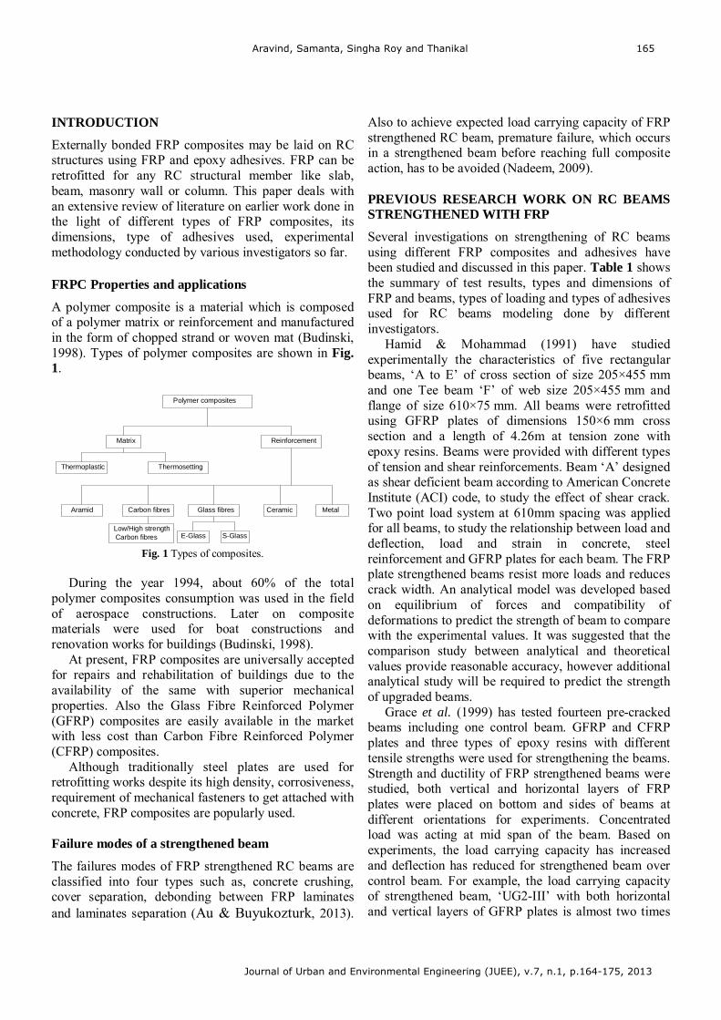
Aravind, Samanta, Singha Roy and Thanikal
Journal of Urban and Environmental Engineering (JUEE), v.7, n.1, p.164-175, 2013
165
INTRODUCTION
Externally bonded FRP composites may be laid on RC structures using FRP and epoxy adhesives. FRP can be retrofitted for any RC structural member like slab, beam, masonry wall or column. This paper deals with an extensive review of literature on earlier work done in the light of different types of FRP composites, its dimensions, type of adhesives used, experimental methodology conducted by various investigators so far. FRPC Properties and applications
A polymer composite is a material which is composed of a polymer matrix or reinforcement and manufactured in the form of chopped strand or woven mat (Budinski, 1998). Types of polymer composites are shown in Fig. 1.
Glass fibres
Polymer composites
Matrix
Aramid
Thermoplastic
Low/High strength Carbon fibres E-Glass
Carbon fibres
Thermosetting
Reinforcement
S-Glass
Ceramic Metal
Fig. 1 Types of composites.
During the year 1994, about 60% of the total
polymer composites consumption was used in the field of aerospace constructions. Later on composite materials were used for boat constructions and renovation works for buildings (Budinski, 1998).
At present, FRP composites are universally accepted for repairs and rehabilitation of buildings due to the availability of the same with superior mechanical properties. Also the Glass Fibre Reinforced Polymer (GFRP) composites are easily available in the market with less cost than Carbon Fibre Reinforced Polymer (CFRP) composites.
Although traditionally steel plates are used for retrofitting works despite its high density, corrosiveness, requirement of mechanical fasteners to get attached with concrete, FRP composites are popularly used. Failure modes of a strengthened beam
The failures modes of FRP strengthened RC beams are classified into four types such as, concrete crushing, cover separation, debonding between FRP laminates and laminates separation (Au & Buyukozturk, 2013).
Also to achieve expected load carrying capacity of FRP strengthened RC beam, premature failure, which occurs in a strengthened beam before reaching full composite action, has to be avoided (Nadeem, 2009). PREVIOUS RESEARCH WORK ON RC BEAMS STRENGTHENED WITH FRP
Several investigations on strengthening of RC beams using different FRP composites and adhesives have been studied and discussed in this paper. Table 1 shows the summary of test results, types and dimensions of FRP and beams, types of loading and types of adhesives used for RC beams modeling done by different investigators.
Hamid & Mohammad (1991) have studied experimentally the characteristics of five rectangular beams, ‘A to E’ of cross section of size 205×455 mm and one Tee beam ‘F’ of web size 205×455 mm and flange of size 610×75 mm. All beams were retrofitted using GFRP plates of dimensions 150×6 mm cross section and a length of 4.26m at tension zone with epoxy resins. Beams were provided with different types of tension and shear reinforcements. Beam ‘A’ designed as shear deficient beam according to American Concrete Institute (ACI) code, to study the effect of shear crack. Two point load system at 610mm spacing was applied for all beams, to study the relationship between load and deflection, load and strain in concrete, steel reinforcement and GFRP plates for each beam. The FRP plate strengthened beams resist more loads and reduces crack width. An analytical model was developed based on equilibrium of forces and compatibility of deformations to predict the strength of beam to compare with the experimental values. It was suggested that the comparison study between analytical and theoretical values provide reasonable accuracy, however additional analytical study will be required to predict the strength of upgraded beams.
Grace et al. (1999) has tested fourteen pre-cracked beams including one control beam. GFRP and CFRP plates and three types of epoxy resins with different tensile strengths were used for strengthening the beams. Strength and ductility of FRP strengthened beams were studied, both vertical and horizontal layers of FRP plates were placed on bottom and sides of beams at different orientations for experiments. Concentrated load was acting at mid span of the beam. Based on experiments, the load carrying capacity has increased and deflection has reduced for strengthened beam over control beam. For example, the load carrying capacity of strengthened beam, ‘UG2-III’ with both horizontal and vertical layers of GFRP plates is almost two times
Aravind, Samanta, Singha Roy and Thanikal
Journal of Urban and Environmental Engineering (JUEE), v.7, n.1, p.164-175, 2013
166
that of the control beam. Also it was mentioned that, high value of factor of safety is to be taken in design, since all the FRP strengthened beams were subjected to brittle failure. Also the beam was strengthened with vertical layers over entire span of the beam to resist diagonal cracks.
Tarek & Al-Salloum (2001) have strengthened and tested the three beams with GFRP and two with CFRP composites using epoxy resins and test results were compared with a control beam. One, 2 and 4 numbers of layer of 1.3 mm GFRP and 1 and 2 layers of 1 mm CFRP were used for externally strengthening beams. All beams were reinforced with 310 mm diameter bars at tension zone, 16 mm diameter bar at compression zone and 2 legged 8 mm diameter stirrups at 100 mm c/c. The developed equations based on ACI code for moment capacity of strengthened beams, thickness of FRP are theoretically verified with experimental values. Two point loads with spacing 200 mm were applied for experiments. All beams were failed by concrete crushing at compression zone. It was concluded that the flexural strength of strengthened beams using FRP laminates at tension zone, more than that of control beam. Outcome results based on computational model which has been presented by the author were performed well in the prediction of experimental results.
Abdelhady et al. (2006) has studied on the influence of hybrid FRP wrapping techniques on the reinforced concrete Tee beams. Seven beams were tested including one control specimen. CFRP, GFRP and both laminates were provided at different locations, directions and connected with a beam by epoxy adhesives. The corners of the beams are rounded at radius of 15 mm to fix ‘U’ wrap of thickness 0.117 and 0.135 mm for CFRP & GFRP respectively. The beams were tested with two point cyclic loads acting at a distance of 750 mm. The ultimate loads for strengthened beams are between 16.5 and 69.7 percent than controlled beam. Strain compatibility approach was used for ultimate load predictions and integration of the curvature along the span for deflection calculations. Theoretical values were compared with experimental values and it shows good correlation. The characteristics of beams can be determined by strain compatibility approach accurately.
Chiew et al. (2007) focused on the experimental work on two unstrengthened and ten flexurally strengthened beams using GFRP laminates. Total beams grouped into two, such as ‘A’ and ‘B’ based on points of application of loads. Spacing between two point loads are 1000 mm and 400 mm for group A and B respectively. Number of layers and length of GFRP laminates were varied for strengthened beams. Epoxy resin adhesive was used for attaching GFRP with beam. This experimental study shows that, two unstrengthened beams were failed by flexure and strengthened beams were failed by laminates debonding. The strength and stiffness were increased significantly for flexurally
strengthened beams. The progress of debonding started from the point of loading towards the supports. Analysis of interface relationship between concrete and laminates was done by finite element method. Moment-deflection relationships for strengthened beams calculated by FE analysis were moderately well, since during the analysis, the interfacial debonding of FRP from the beam is negligible.
Pannirselvam et al. (2008) tested nine beams out of which six beams were strengthened with GFRP and three were controlled beams. A model was developed with the data available from seven beams by General Regression Neural Network (GRNN) technique using MATLAB and two beam results were used for testing the model. Also varied tension reinforcement for beams 1, 2 and 3 such as 0.419, 0.603 and 0.905 percent respectively was studied. Two concentrated loads were applied on the beam at a spacing of 933 mm. Load and deflections at first crack, yield and ultimate levels are measured for all beams. 3 and 5 mm GFRP plates and epoxy adhesives were used for strengthening RC beams. First crack load was increased for beams by increasing thickness of plates. Yield strengths for strengthened beams were increased by a maximum of 76.49 and 111.79 percent for 3 and 5 mm thick plates.
Jumaat & Alam (2008) also worked on three beams of dimensions 125×250×2000 mm such as A1, B1 & C1. A1 was kept as control beam; B1 and C1 were strengthened by steel plate of dimensions 2.76×73×1900 mm and CFRP laminates of dimensions 1.2×80×1900 mm respectively. Compression and shear reinforcements were provided only on ends of a beam. Those dimensions were designed based on simplified stress block method of BS 8110. Steel plate and CFRP laminate (SikaCarboDur S812) were provided full length off the beams to maximize the strengthening effects. From the experiments, it was found that the controlled beam A1 failed by flexure, while B1 failed by debonding followed by concrete cover separation and the beam C1 failed by debonding. Experimental results were compared with the values obtained by finite element analysis. From the comparison study it was found that those two results were almost equal for control beam, but failure loads for strengthened beams by finite element analysis were more than experimental results. The reason was, the FE analysis was done based on assumption of bond between strengthening materials and concrete surface was perfect.
In another research Sundarraja et al. (2008) tested thirteen beams including five control beams. All beams were divided into three sets based on wrapping such as five control beam ‘C’ without wrapping, four beams with vertical strips ‘V’ and four ‘U’ wrap strip beams. For ‘V’ group beams, strips were provided at a width of 15 mm and c/c spacing of 45 mm. The widths of these GFRP strips were designed based on ACI recommendations. GFRP composites were connected
Aravind, Samanta, Singha Roy and Thanikal
Journal of Urban and Environmental Engineering (JUEE), v.7, n.1, p.164-175, 2013
167
with beams using epoxy resins and hardener. The wrapped beams resist more load than controlled beams and the vertical GFRP strips prevent diagonal cracks significantly. It was concluded that the recommendations provided by ACI code can be used for design of strips for retrofitted works.
Amer & Mohammed (2009) analyzed theoretically by finite elements methods by ANSYS package on FRP retrofitted beams. Experiment investigated six shear deficient rectangular beams of cross section 150×250 mm including two control beams B1 and B2. Epoxy resins were used to retrofit Carbon or Glass fiber reinforced polymers with RC beams. For B1C-90 type, one layer of 1.6 mm CFRP laminates was provided perpendicular to the longitudinal axis of a beam. B1G-90 beam was similar to previous type but two layers of 2.1 mm GFRP were used. For B2C-90 type, one layer of 0.18 mm CFRP composites was wrapped perpendicular to the longitudinal axis of a beam. For B2C-90-0 type, two layers of 0.18 mm CFRP composites were wrapped on two directions such as 90° and 0° to the longitudinal axis of a beam. Effect of directions of FRP composites on RC beams were studied, since it is an orthotropic material. The ultimate shear strength values of retrofitted beams by experimental values were good agreement with shear strength analyzed by finite element model, concluding that the carbon fibres were resisting more load than glass fibres retrofitted with beams.
Nadeem (2009) experimentally investigated six beams on strengthening of RC beams in flexure and shear using 1 mm thick CFRP sheet and epoxy resins. The beams were categorized into two groups such as 1 and 2. Group 1 beams were weak in flexure and strong in shear and group 2 beams were weak in shear and strong in flexure. BCF and BCS were control beams from each group. For BFS-1&2 beams, one layer of CFRP was fixed at bottom and for BFS-2, additional ‘U’ wrap attached at ends of a beam. For BSS-1&2 beams, vertical and inclined CFRP strips were attached on the sides of a beam. Concentrated loads at a distance of 500 mm were applied on all beams. It was found that, BCF, BCS and BFS-2 were failed by flexure, shear and concrete crushing at compression zone respectively. Remaining three beams were failed by debonding of laminates. Also it was observed that beam with CFRP sheets at bottom & ‘U’ shaped anchorages resisted more flexural load than BFS-1, and beam with inclined strips resisted more shear than vertical strips.
Pan et al. (2010) examined eight beams to study the effect of flexural and shear cracks on FRP debonding. The beams were grouped into two, on first group, opening in the shape of notches developed at tension zone along the length of the beam to avoid the secondary cracks in the shear or flexural portion (B1-B4). Single notch for beams B1, B2 and double notches for beams B3, B4 were provided at bottom and GFRP
plates were connected at sides and bottom of the beams. Multiple cracks were developed for group two beams by preloaded technique (B5-B8). For beam B5 two shallow notches were provided at bottom. B6 and B8 were un-notched and GFRP plates were provided at bottom of the beams. B7 was un-notched but flexural or shear cracks were developed. All beams were anchored with ‘U’ shaped FRP plates. A mathematical model has been developed for determination of stress strain distribution along the FRP corresponding to number of secondary cracks and major cracks. Beams were strengthened using 0.22 mm thick GFRP composites with epoxy resins. Two point loading system is applied at a loading span of 300 mm. All beams were failed by FRP debonding. The average load carrying capacity of second group beams are much more than that of beams from first group. Developed mathematical model has been validated by the data which are available from experimental results, and it revealed that calculated stress and strain values using mathematical model were matched well with the experimental values.
Yasmeen et al. (2011) investigated twelve beams which were divided into two groups such as RF and RS. In RF group beams, reinforcements were deficient in flexure and shear and the beams were flexurally strengthened by 50 mm CFRP plates at soffit of the beam by varying its lengths after preloading. In RS group, the beams were shear strengthened by 50 mm CFRP strips at sides of the beam at a spacing of 100 mm c/c and it is not provided at middle third 520 mm portion. Out of which four beams were tested as control beams, two from RF and two from RS group. Thickness of CFRP used is 1.2 mm and number of layer is 1 for both beam groups and epoxy resin is used to fix the beam. Two point loads were applied at a distance of 520 mm. After loading, it has been noted that crack width of the strengthened beam has been decreased by comparing control specimen. All the strengthened beams were failed by brittle and followed by sudden CFRP debonding from the concrete. Control beams RF and RS were failed by flexure and shear. Two equal beams were casted in each set and the mean value has been considered as maximum load. Also it was found that load carrying capacity of strengthened beams was increased from 7 upto 33 percent in flexure and about 23 percent in shear.
Recently, Heshmi & Al-Mahaidi (2012) have presented an experimental work on RC beams retrofitted with CFRP textile and fabrics using cement based adhesives at high temperature. Testing of seven beams at cross sectional area of 120×180 mm was done. The cement based adhesives consists of OPC, micro cement at ratio of 1:4, super plasticizer and silica fume. The beams were tested at two types such as beams subjected to high temperature at constant service load and failure load at constant temperature. The reinforced concrete beams retrofitted using epoxy adhesives were
Aravind, Samanta, Singha Roy and Thanikal
Journal of Urban and Environmental Engineering (JUEE), v.7, n.1, p.164-175, 2013
168
failed by CFRP delamination at a temperature of 462°C and performed similar to normal beam. On the other hand, beam retrofitted using cement based adhesives has resisted 844°C and this value is almost equal to the failure temperature of RC beams. The performances of beams such as crack pattern and strain distribution were theoretically determined by finite element analysis and values were compared with the test results, reveals that the two results are closely correlated.
Most recently Dong et al. (2013) has conducted test on fourteen beams divided into two groups such as flexural (CR) and flexural shear strengthening (SR) using FRP sheets. A study on the effect of beam size and concrete cover to the reinforcements on the flexural strength of strengthened beam was conducted. Concrete grades are not specified for CR group beams and it is common for that group, since beams were tested with varying cover thickness and reinforcement percentage. 28 days compressive strength for five beams of SR group was 22.8 MPa and two beams of same group was 31.3 MPa. One layer of GFRP sheet with size 1500×50×0.273 mm and two layers of CFRP sheets of same length and width and 0.111 mm thickness were applied on bottom and sides of the beams. Two point load system were applied on beams at a spacing of 500 mm. While loading, three numbers of LVDT were fixed at bottom of beams at different locations to measure deflections. Experimental results show that, ultimate loads for flexural strengthened beams increased between 41 and 125 percent over control beam and shear capacity of strengthened beams increased by 31 and 74 percent. Based on existing data from previous studies, theoretical values were calculated and correlated with experimental values.
COMMENTS ON THE PRESENT STATE OF ART. The above review of literatures on the field of strengthening of RC beams show that the researchers have tried GFRP, CFRP or hybrid laminates with different thicknesses and number of layers. Most of the research works have compared the experimental values with theoretical values. Out of fourteen papers, for theoretical analysis, Pannirselvam et al. (2008) have used General Regression Neural Network (GRNN) technique using MATLAB neural network, (Amer & Mohammed, 2009; Hashemi & Al-Mahaidi, 2012; Jumaat & Alam, 2008) and Sing et al. (2007) have used finite element analysis, in which (Hamid & Mohammad, 1991) has developed analytical model based on equilibrium of forces and compatibility of
deformations, equations for moment capacity of strengthened beams. Also Sundarraja et al. (2008) has designed thickness of FRP laminate based on ACI code, while Abdelhady et al. (2006) has used strain compatibility approach for ultimate load predictions and deflection calculations.
PROBLEMS OF STRENGTHENING RC BEAMS The study indicates that researchers have used FRP plane laminates at different number of layers. Authors (Hamid & Mohammad, 1991; Pannirselvam et al., 2008; Jumaat & Alam, 2008; Sundarraja, 2008; Yasmeen et al., 2011; Heshmi & Al-Mahaidi, 2012) have used one layer of laminates, authors (Amer & Mohammed, 2009; Jinlong et al., 2010; Jiangfeng et al., 2013) have tried up to two layers of laminates, while authors Abdelhady et al. (2006) and Sing et al. (2007) has attached three layers and authors Grace et al. (1999) and Tarek & Al-Salloum (2001) used upto four layers.
According to ACI code assumptions, the bond between laminates and concrete surface is perfect (ACI 440.2R-08). But most of the cases discussed in failure modes of a strengthened beam, the failure of beams occurred due to debonding of laminates from concrete surface. In those cases, the beams failed by premature failure which means, beams failed under the initial load. Also it has been noticed that, failure due to debonding of laminates occurs for beams retrofitted only at the bottom.
From theoretical analysis, the researchers have used only one tool for model development such as either finite element analysis or neural network. PROPOSED METHOD OF STRENGTHENING THE RC BEAM To overcome the problem discussed in this paper, in the proposed work, FRP composites are used to develop a new profile and investigations for its physical dimensions and structural behaviors, in flexural members. FRP laminates will be provided with full length of the beam to take into account shear and bending. To avoid premature failure, FRP laminates are provided at bottom and are extended to the sides also. Most of the authors have used epoxy resins for attaching FRP laminates with concrete surface due to its superior property by comparing other adhesives. The same resins will be used for proposed work. Thirteen authors out of the reviewed literatures have used two point load system for their experimental setup.
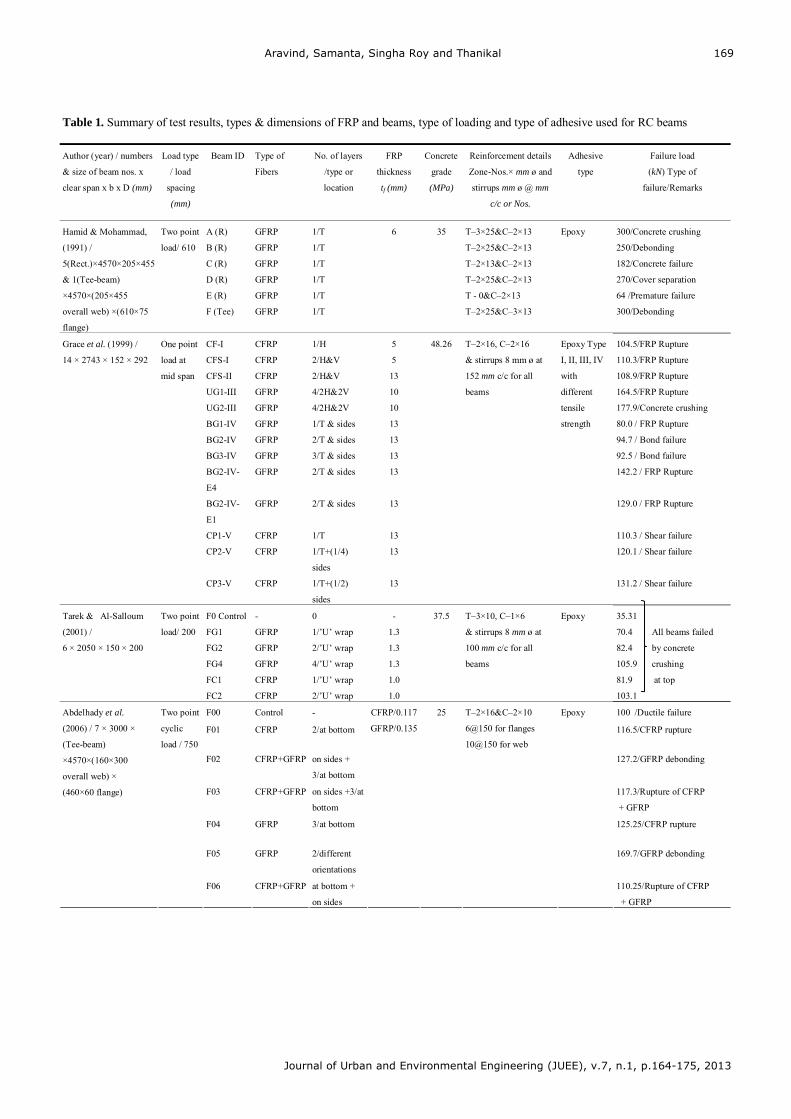
Aravind, Samanta, Singha Roy and Thanikal
Journal of Urban and Environmental Engineering (JUEE), v.7, n.1, p.164-175, 2013
169
Table 1. Summary of test results, types & dimensions of FRP and beams, type of loading and type of adhesive used for RC beams
Author (year) / numbers
& size of beam nos. x
clear span x b x D (mm)
Load type
/ load
spacing
(mm)
Beam ID Type of
Fibers
No. of layers
/type or
location
FRP
thickness
tf (mm)
Concrete
grade
(MPa)
Reinforcement details
Zone-Nos.× mm ø and
stirrups mm ø @ mm
c/c or Nos.
Adhesive
type
Failure load
(kN) Type of
failure/Remarks
Hamid & Mohammad,
(1991) /
5(Rect.)×4570×205×455
& 1(Tee-beam)
×4570×(205×455
overall web) ×(610×75
flange)
Two point
load/ 610
A (R)
B (R)
C (R)
D (R)
E (R)
F (Tee)
GFRP
GFRP
GFRP
GFRP
GFRP
GFRP
1/T
1/T
1/T
1/T
1/T
1/T
6 35 T–3×25&C–2×13
T–2×25&C–2×13
T–2×13&C–2×13
T–2×25&C–2×13
T - 0&C–2×13
T–2×25&C–3×13
Epoxy
300/Concrete crushing
250/Debonding
182/Concrete failure
270/Cover separation
64 /Premature failure
300/Debonding
Grace et al. (1999) /
14 × 2743 × 152 × 292
One point
load at
mid span
CF-I
CFS-I
CFS-II
UG1-III
UG2-III
BG1-IV
BG2-IV
BG3-IV
BG2-IV-
E4
BG2-IV-
E1
CP1-V
CP2-V
CP3-V
CFRP
CFRP
CFRP
GFRP
GFRP
GFRP
GFRP
GFRP
GFRP
GFRP
CFRP
CFRP
CFRP
1/H
2/H&V
2/H&V
4/2H&2V
4/2H&2V
1/T & sides
2/T & sides
3/T & sides
2/T & sides
2/T & sides
1/T
1/T+(1/4)
sides
1/T+(1/2)
sides
5
5
13
10
10
13
13
13
13
13
13
13
13
48.26 T–2×16, C–2×16
& stirrups 8 mm ø at
152 mm c/c for all
beams
Epoxy Type
I, II, III, IV
with
different
tensile
strength
104.5/FRP Rupture
110.3/FRP Rupture
108.9/FRP Rupture
164.5/FRP Rupture
177.9/Concrete crushing
80.0 / FRP Rupture
94.7 / Bond failure
92.5 / Bond failure
142.2 / FRP Rupture
129.0 / FRP Rupture
110.3 / Shear failure
120.1 / Shear failure
131.2 / Shear failure
Tarek & Al-Salloum
(2001) /
6 × 2050 × 150 × 200
Two point
load/ 200
F0 Control
FG1
FG2
FG4
FC1
FC2
-
GFRP
GFRP
GFRP
CFRP
CFRP
0
1/’U’ wrap
2/’U’ wrap
4/’U’ wrap
1/’U’ wrap
2/’U’ wrap
-
1.3
1.3
1.3
1.0
1.0
37.5 T–3×10, C–1×6
& stirrups 8 mm ø at
100 mm c/c for all
beams
Epoxy
35.31
70.4
82.4
105.9
81.9
103.1
All beams failed
by concrete
crushing
at top
F00 Control - 100 /Ductile failure
F01 CFRP 2/at bottom 116.5/CFRP rupture
F02
CFRP+GFRP on sides +
3/at bottom
127.2/GFRP debonding
F03
CFRP+GFRP
on sides +3/at
bottom
117.3/Rupture of CFRP
+ GFRP
F04 GFRP 3/at bottom 125.25/CFRP rupture
F05
GFRP
2/different
orientations
169.7/GFRP debonding
Abdelhady et al.
(2006) / 7 × 3000 ×
(Tee-beam)
×4570×(160×300
overall web) ×
(460×60 flange)
Two point
cyclic
load / 750
F06
CFRP+GFRP at bottom +
on sides
CFRP/0.117
GFRP/0.135
25 T–2×16&C–2×10
6@150 for flanges
10@150 for web
Epoxy
110.25/Rupture of CFRP
+ GFRP
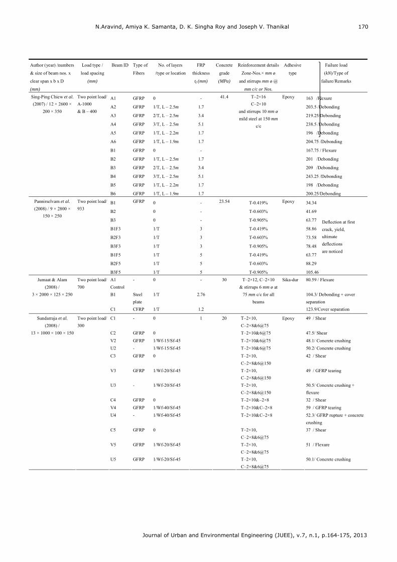
N.Aravind, Amiya K. Samanta, D. K. Singha Roy and Joseph V. Thanikal
Journal of Urban and Environmental Engineering (JUEE), v.7, n.1, p.164-175, 2013
170
Author (year) /numbers
& size of beam nos. x
clear span x b x D
(mm)
Load type /
load spacing
(mm)
Beam ID Type of
Fibers
No. of layers
/type or location
FRP
thickness
tf (mm)
Concrete
grade
(MPa)
Reinforcement details
Zone-Nos.× mm ø
and stirrups mm ø @
mm c/c or Nos.
Adhesive
type
Failure load
(kN)/Type of
failure/Remarks
Sing-Ping Chiew et al.
(2007) / 12 × 2600 ×
200 × 350
Two point load/
A-1000
& B – 400
A1
A2
A3
A4
A5
A6
B1
B2
B3
B4
B5
B6
GFRP
GFRP
GFRP
GFRP
GFRP
GFRP
GFRP
GFRP
GFRP
GFRP
GFRP
GFRP
0
1/T, L – 2.5m
2/T, L – 2.5m
3/T, L – 2.5m
1/T, L – 2.2m
1/T, L – 1.9m
0
1/T, L – 2.5m
2/T, L – 2.5m
3/T, L – 2.5m
1/T, L – 2.2m
1/T, L – 1.9m
-
1.7
3.4
5.1
1.7
1.7
-
1.7
3.4
5.1
1.7
1.7
41.4 T–2×16
C–2×10
and stirrups 10 mm ø
mild steel at 150 mm
c/c
Epoxy
163 /Flexure
203.5 /Debonding
219.25/Debonding
238.5 /Debonding
196 /Debonding
204.75 /Debonding
167.75 / Flexure
201 /Debonding
209 /Debonding
243.25 /Debonding
198 /Debonding
200.25/Debonding
Pannirselvam et al.
(2008) / 9 × 2800 ×
150 × 250
Two point load/
933 B1
B2
B3
B1F3
B2F3
B3F3
B1F5
B2F5
B3F5
GFRP
0
0
0
1/T
1/T
1/T
1/T
1/T
1/T
-
-
-
3
3
3
5
5
5
23.54 T-0.419%
T-0.603%
T-0.905%
T-0.419%
T-0.603%
T-0.905%
T-0.419%
T-0.603%
T-0.905%
Epoxy
34.34
41.69
63.77
58.86
73.58
78.48
63.77
88.29
105.46
Deflection at first
crack, yield,
ultimate
deflections
are noticed
A1
Control
- 0 - 80.59 / Flexure
B1 Steel
plate
1/T
2.76
104.3/ Debonding + cover
separation
Jumaat & Alam
(2008) /
3 × 2000 × 125 × 250
Two point load/
700
C1 CFRP 1/T 1.2
30 T–2×12, C–2×10
& stirrups 6 mm ø at
75 mm c/c for all
beams
Sika-dur
123.9/Cover separation
C1
- 0 T–2×10,
C–2×8&6@75
49 / Shear
C2 GFRP 0 T–2×10&6@75 47.5/ Shear
V2 GFRP 1/Wf-15/Sf-45 T–2×10&6@75 48.1/ Concrete crushing
U2 - 1/Wf-15/Sf-45 T–2×10&6@75 50.2/ Concrete crushing
C3
GFRP 0 T–2×10,
C–2×8&6@150
42 / Shear
V3
GFRP 1/Wf-20/Sf-45 T–2×10,
C–2×8&6@150
49 / GFRP tearing
U3
- 1/Wf-20/Sf-45 T–2×10,
C–2×8&6@150
50.5/ Concrete crushing +
flexure
C4 GFRP 0 T–2×10&–2×8 32 / Shear
V4 GFRP 1/Wf-40/Sf-45 T–2×10&C–2×8 59 / GFRP tearing
U4 - 1/Wf-40/Sf-45 T–2×10&C–2×8 52.3/ GFRP rupture + concrete
crushing
C5
GFRP 0 T–2×10,
C–2×8&6@75
37 / Shear
V5
GFRP 1/Wf-20/Sf-45 T–2×10,
C–2×8&6@75
51 / Flexure
Sundarraja et al.
(2008) /
13 × 1000 × 100 × 150
Two point load/
300
U5 GFRP 1/Wf-20/Sf-45
1 20
T–2×10,
C–2×8&6@75
Epoxy
50.1/ Concrete crushing

Aravind, Samanta, Singha Roy and Thanikal
Journal of Urban and Environmental Engineering (JUEE), v.7, n.1, p.164-175, 2013
171
Author (year)
/numbers & size of
beam nos. x clear span
x b x D (mm)
Load type /
load spacing
(mm)
Beam ID Type
of
Fibers
No. of layers /type or
location
FRP
thickness
tf (mm)
Concrete
grade
(MPa)
Reinforcement details
Zone-Nos.× mm ø and
stirrups mm ø @ mm
c/c or Nos.
Adhesive
type
Failure load
(kN) / Type of
failure/Remarks
B1 0 - 27.54 T–2×13&C–2×10 69
B1C-90
CFRP 1/Uni directional
1.6 27.54 T–2×13&C–2×10
125
BIG-90
GFRP 2/Uni directional 2.1 27.54 T–2×13&C–2×10
116
B2
- 0 - 31 T–2×25&C–2×9 416
B2C-90
CFRP 1/90° to LA
0.18 31 T–2×25&C–2×9
435
Amer & Mohammed,
(2009) / 6 × 2440 ×
150 × 250
Two point
load/1700
B2C-90-0
CFRP 2/1 layer at 90° & 1
layer on both sides of
web 0° to the LA
0.18 31 T–2×25&C–2×9
Epoxy
445
Experimental ultimate
loads have been
compare with
numerical loads and
mode of failure not
discussed.
Stirrups 10 mm ø at
600 mm c/c used for
B1 type beams &
9 mm ø at 300 mm c/c
used for B2 type
beams
BCF
Control
-
0
-
T–3×14&C–1×6 197.2 / Flexure
BFS-1 CFRP 1/T 1 T–3×14&C–1×6 241.5 / Debonding
BFS-2
CFRP 1/T+1/U wrap 1 T–3×14&C–1×6
255.2 / Concrete crushing at top
BCS
Control
- 0 - T–3×20&C–1×6
81.98 / Shear
BSS-1
CFRP 1/Vertical strips on
sides
1 T–3×20&C–1×6
95.97 / Debonding
Nadeem (2009) /
6 × 2000 × 200 × 300
Two point
load/ 500
BSS-2 CFRP 1/Inclined
strips on sides
1
35
T–3×20&C–1×6
and stirrups 10 mm ø at
100 mm c/c for first 3
beams & 6 mm ø at
150 mm c/c for
remaining 3 beams
Epoxy
111.01 / Debonding
Jinlong et al. (2010) /
8×1800×150 × 200
Two point
load/ 300 B1
B2
B3
B4
B5
B6
B7
B8
GFRP
GFRP
GFRP
GFRP
GFRP
GFRP
GFRP
GFRP
2/T
L-1.7 m
For all beams
0.22 42.9 T–2×10
8@14Nos.
Epoxy
28.43
27.69
27.71
27.52
79.61
77.00
76.34
75.31
All beams are failed
by FRP debonding
2×RF
Control 0 - 118 / flexure
2×RF1 CFRP 1/L-1.56m, b-50 1.2 166 / debonding
2×RF2 CFRP 1/L-1.04m, b-50 1.2 142 / debonding
2×RF3 CFRP 1/L-0.52m, b-50 1.2 128 / debonding
2×RS Control 0 - 220 / shear
Yasmeen et al. (2011)
/ 12×1560× 150 × 300
Two point
load/ 520
2×RS1 CFRP 1/Wf-50/Sf-100 1.2
29 RF
T–2×12,
C–2×10 & 6@100
RS
T–2×18,
C–2×10 & 6@400
Epoxy
270 / debonding
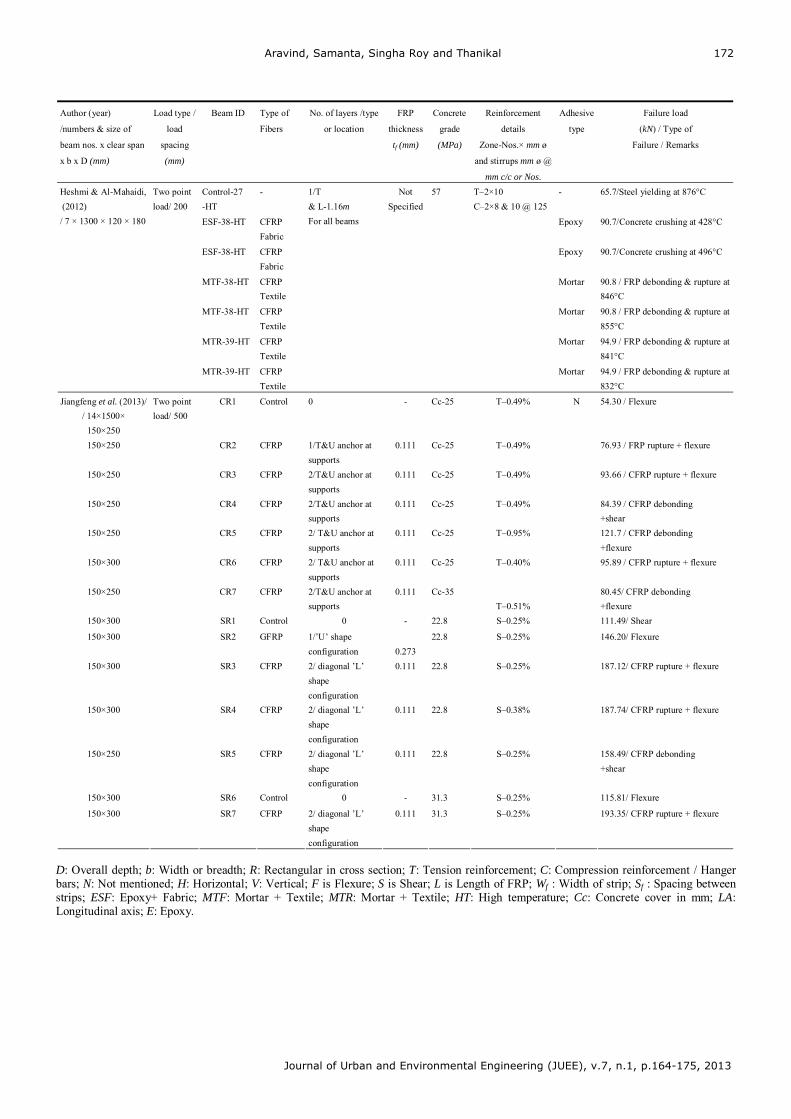
Aravind, Samanta, Singha Roy and Thanikal
Journal of Urban and Environmental Engineering (JUEE), v.7, n.1, p.164-175, 2013
172
Author (year)
/numbers & size of
beam nos. x clear span
x b x D (mm)
Load type /
load
spacing
(mm)
Beam ID Type of
Fibers
No. of layers /type
or location
FRP
thickness
tf (mm)
Concrete
grade
(MPa)
Reinforcement
details
Zone-Nos.× mm ø
and stirrups mm ø @
mm c/c or Nos.
Adhesive
type
Failure load
(kN) / Type of
Failure / Remarks
Control-27
-HT
-
-
65.7/Steel yielding at 876°C
ESF-38-HT
CFRP
Fabric
Epoxy
90.7/Concrete crushing at 428°C
ESF-38-HT
CFRP
Fabric
Epoxy
90.7/Concrete crushing at 496°C
MTF-38-HT
CFRP
Textile
Mortar
90.8 / FRP debonding & rupture at
846°C
MTF-38-HT
CFRP
Textile
Mortar
90.8 / FRP debonding & rupture at
855°C
MTR-39-HT CFRP
Textile
Mortar
94.9 / FRP debonding & rupture at
841°C
Heshmi & Al-Mahaidi,
(2012)
/ 7 × 1300 × 120 × 180
Two point
load/ 200
MTR-39-HT CFRP
Textile
1/T
& L-1.16m
For all beams
Not
Specified
57 T–2×10
C–2×8 & 10 @ 125
Mortar
94.9 / FRP debonding & rupture at
832°C
Jiangfeng et al. (2013)/
/ 14×1500×
150×250
CR1 Control 0 - Cc-25 T–0.49% 54.30 / Flexure
150×250
CR2 CFRP
1/T&U anchor at
supports
0.111 Cc-25
T–0.49%
76.93 / FRP rupture + flexure
150×250
CR3 CFRP
2/T&U anchor at
supports
0.111
Cc-25
T–0.49%
93.66 / CFRP rupture + flexure
150×250
CR4 CFRP
2/T&U anchor at
supports
0.111
Cc-25
T–0.49% 84.39 / CFRP debonding
+shear
150×250
CR5 CFRP
2/ T&U anchor at
supports
0.111
Cc-25
T–0.95%
121.7 / CFRP debonding
+flexure
150×300
CR6 CFRP
2/ T&U anchor at
supports
0.111
Cc-25
T–0.40%
95.89 / CFRP rupture + flexure
150×250
CR7 CFRP
2/T&U anchor at
supports
0.111
Cc-35
T–0.51%
80.45/ CFRP debonding
+flexure
150×300 SR1 Control 0 - 22.8 S–0.25% 111.49/ Shear
150×300
SR2 GFRP 1/’U’ shape
configuration
0.273
22.8 S–0.25% 146.20/ Flexure
150×300
SR3 CFRP
2/ diagonal ’L’
shape
configuration
0.111
22.8 S–0.25% 187.12/ CFRP rupture + flexure
150×300
SR4 CFRP
2/ diagonal ’L’
shape
configuration
0.111
22.8 S–0.38%
187.74/ CFRP rupture + flexure
150×250
SR5 CFRP
2/ diagonal ’L’
shape
configuration
0.111
22.8 S–0.25%
158.49/ CFRP debonding
+shear
150×300 SR6 Control 0 - 31.3 S–0.25% 115.81/ Flexure
150×300
Two point
load/ 500
SR7 CFRP
2/ diagonal ’L’
shape
configuration
0.111
31.3 S–0.25%
N
193.35/ CFRP rupture + flexure
D: Overall depth; b: Width or breadth; R: Rectangular in cross section; T: Tension reinforcement; C: Compression reinforcement / Hangerbars; N: Not mentioned; H: Horizontal; V: Vertical; F is Flexure; S is Shear; L is Length of FRP; Wf : Width of strip; Sf : Spacing between strips; ESF: Epoxy+ Fabric; MTF: Mortar + Textile; MTR: Mortar + Textile; HT: High temperature; Cc: Concrete cover in mm; LA:Longitudinal axis; E: Epoxy.
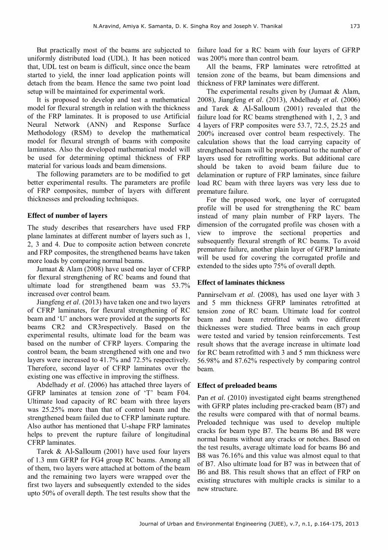
N.Aravind, Amiya K. Samanta, D. K. Singha Roy and Joseph V. Thanikal
Journal of Urban and Environmental Engineering (JUEE), v.7, n.1, p.164-175, 2013
173
But practically most of the beams are subjected to uniformly distributed load (UDL). It has been noticed that, UDL test on beam is difficult, since once the beam started to yield, the inner load application points will detach from the beam. Hence the same two point load setup will be maintained for experimental work.
It is proposed to develop and test a mathematical model for flexural strength in relation with the thickness of the FRP laminates. It is proposed to use Artificial Neural Network (ANN) and Response Surface Methodology (RSM) to develop the mathematical model for flexural strength of beams with composite laminates. Also the developed mathematical model will be used for determining optimal thickness of FRP material for various loads and beam dimensions.
The following parameters are to be modified to get better experimental results. The parameters are profile of FRP composites, number of layers with different thicknesses and preloading techniques.
Effect of number of layers
The study describes that researchers have used FRP plane laminates at different number of layers such as 1, 2, 3 and 4. Due to composite action between concrete and FRP composites, the strengthened beams have taken more loads by comparing normal beams.
Jumaat & Alam (2008) have used one layer of CFRP for flexural strengthening of RC beams and found that ultimate load for strengthened beam was 53.7% increased over control beam.
Jiangfeng et al. (2013) have taken one and two layers of CFRP laminates, for flexural strengthening of RC beam and ‘U’ anchors were provided at the supports for beams CR2 and CR3respectively. Based on the experimental results, ultimate load for the beam was based on the number of CFRP layers. Comparing the control beam, the beam strengthened with one and two layers were increased to 41.7% and 72.5% respectively. Therefore, second layer of CFRP laminates over the existing one was effective in improving the stiffness.
Abdelhady et al. (2006) has attached three layers of GFRP laminates at tension zone of ‘T’ beam F04. Ultimate load capacity of RC beam with three layers was 25.25% more than that of control beam and the strengthened beam failed due to CFRP laminate rupture. Also author has mentioned that U-shape FRP laminates helps to prevent the rupture failure of longitudinal CFRP laminates.
Tarek & Al-Salloum (2001) have used four layers of 1.3 mm GFRP for FG4 group RC beams. Among all of them, two layers were attached at bottom of the beam and the remaining two layers were wrapped over the first two layers and subsequently extended to the sides upto 50% of overall depth. The test results show that the
failure load for a RC beam with four layers of GFRP was 200% more than control beam.
All the beams, FRP laminates were retrofitted at tension zone of the beams, but beam dimensions and thickness of FRP laminates were different.
The experimental results given by (Jumaat & Alam, 2008), Jiangfeng et al. (2013), Abdelhady et al. (2006) and Tarek & Al-Salloum (2001) revealed that the failure load for RC beams strengthened with 1, 2, 3 and 4 layers of FRP composites were 53.7, 72.5, 25.25 and 200% increased over control beam respectively. The calculation shows that the load carrying capacity of strengthened beam will be proportional to the number of layers used for retrofitting works. But additional care should be taken to avoid beam failure due to delamination or rupture of FRP laminates, since failure load RC beam with three layers was very less due to premature failure.
For the proposed work, one layer of corrugated profile will be used for strengthening the RC beam instead of many plain number of FRP layers. The dimension of the corrugated profile was chosen with a view to improve the sectional properties and subsequently flexural strength of RC beams. To avoid premature failure, another plain layer of GFRP laminate will be used for covering the corrugated profile and extended to the sides upto 75% of overall depth.
Effect of laminates thickness
Pannirselvam et al. (2008), has used one layer with 3 and 5 mm thickness GFRP laminates retrofitted at tension zone of RC beam. Ultimate load for control beam and beam retrofitted with two different thicknesses were studied. Three beams in each group were tested and varied by tension reinforcements. Test result shows that the average increase in ultimate load for RC beam retrofitted with 3 and 5 mm thickness were 56.98% and 87.62% respectively by comparing control beam.
Effect of preloaded beams
Pan et al. (2010) investigated eight beams strengthened with GFRP plates including pre-cracked beam (B7) and the results were compared with that of normal beams. Preloaded technique was used to develop multiple cracks for beam type B7. The beams B6 and B8 were normal beams without any cracks or notches. Based on the test results, average ultimate load for beams B6 and B8 was 76.16% and this value was almost equal to that of B7. Also ultimate load for B7 was in between that of B6 and B8. This result shows that an effect of FRP on existing structures with multiple cracks is similar to a new structure.
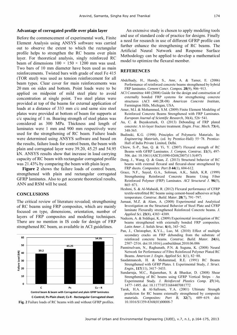
Aravind, Samanta, Singha Roy and Thanikal
Journal of Urban and Environmental Engineering (JUEE), v.7, n.1, p.164-175, 2013
174
Advantage of corrugated profile over plain layer
Before the commencement of experimental work, Finite Element Analysis using ANSYS software was carried out to observe the extent to which the rectangular profile helps to strengthen the RC beams over plain layer. For theoretical analysis, singly reinforced RC beam of dimensions 100 × 150 × 1200 mm was used. Two bars of 10 mm diameter have been used as main reinforcements. Twisted bars with grade of steel Fe 415 (TOR steel) was used as tension reinforcement for all beam types. Clear cover for main reinforcements was 20 mm on sides and bottom. Point loads were to be applied on midpoint of mild steel plate to avoid concentration at single point. Two steel plates were provided at top of the beams for external application of loads at a distance of 333 mm c/c and same size steel plates were provided at bottom of beam for supports at c/c spacing of 1 m. Bearing strength of steel plates was considered as 300 MPa. Thickness and length of laminates were 1 mm and 900 mm respectively were used for the strengthening of RC beam. Failure loads were determined using ANSYS software and based on the results, failure loads for control beam, the beam with plain and corrugated layer were 39.20, 45.25 and 54.95 kN. ANSYS results show that increase in load carrying capacity of RC beam with rectangular corrugated profile was 21.43% by comparing the beam with plain layer.
Figure 2 shows the failure loads of control beam, strengthened with plain and rectangular corrugated GFRP laminates. Also to get accurate theoretical results, ANN and RSM will be used.
CONCLUSIONS
The critical review of literature revealed; strengthening of RC beams using FRP composites, which are mainly focused on type, dimensions, orientation, number of layers of FRP composites and modeling techniques. There are no mention in IS code for design of FRP strengthened RC beam, as available in ACI guidelines.
39.2
45.25
54.95
0
10
20
30
40
50
60
C Ps Cs – R
Failure Load
(kN
)
Control beam & beam with Corrugated and plain GFRP laminates
C‐Control; Ps‐Plain sheet; Cs‐R ‐ Rectangular Corrugated sheet Fig. 2 Failure loads of RC beams with and without GFRP profiles.
An extensive study is chosen to apply modeling tools and use of standard code of practice for designs. Finally a need for research in use of different GFRP profile can further enhance the strengthening of RC beams. The Artificial Neural Network and Response Surface Methodology can be applied to develop a mathematical model to optimize the flexural member. REFERENCES
Abdelhady, H., Hamdy, S., Amr, A. & Tamer, E. (2006) Performance of reinforced concrete beams strengthened by hybrid FRP laminates. Cement Concr. Compos. 28(9), 906−913.
ACI Committee 440 (2008) Guide for the design and construction of externally bonded FRP systems for strengthening concrete structures (ACI 440.2R-08) American Concrete Institute, Farmington Hills, Michigan, USA.
Amer, M.I. & Mohammed, S.M. (2009) Finite Element Modeling of Reinforced Concrete Beams Strengthened with FRP Laminates. European Journal of Scientific Research, 30(4), 526−541.
Au, C. & Buyukozturk, O. (2013) Debonding of FRP plated concrete: A tri-layer fracture treatment. Engin. Frac. Mech. 73(4), 348-365.
Budinski, K.G. (1998) Principles of Polymeric Materials. In: Engineering Materials, (ed. by Prentice-Hall) 55−78. Prentice-Hall of India Private Limited, Delhi.
Chiew, S.-P., Sun, Q. & Yi, Y. (2007) Flexural strength of RC Beams with GFRP Laminates. J. Compos. Construc. 11(5), 497-506. doi: 10.1061/(ASCE)1090-0268(2007)11:5(497)
Dong, J., Wang, Q. & Guan, Z. (2013) Structural behavior of RC beams with external flexural and flexural-shear strengthened by FRP sheets. Composites: Part B 44(1), 604-612.
Grace, N.F., Sayed, G.A., Soliman, A.K., Saleh, K.R. (1999) Strengthening Reinforced Concrete Beams Using Fiber Reinforced Polymer (FRP) Laminates. ACI Structural J. 96(5), 865−871.
Heshmi, S. & Al-Mahaidi, R. (2012) Flexural performance of CFRP textile-retrofitted RC beams using cement-based adhesives at high temperature. Construc. Build. Mater. 28(7), 791−797.
Jumaat, M.Z. & Alam, A. (2008) Experimental and Analytical Investigation on the Structural Behavior of Steel Plate and CFRP laminate Flexurally strengthened Reinforced Concrete beams. J. Applied Sci. 23(8), 4383−4389.
Nadeem, A. & Siddiqui, K. (2009) Experimental investigation of RC beams strengthened with externally bonded FRP composites. Latin Amer. J. Solids Struc. 6(4), 343−362.
Pan, J., Christopher, K.Y.L., Luo, M. (2010) Effect of multiple secondary cracks on FRP debonding from the substrate of reinforced concrete beams. Construc. Build. Mater. 24(6), 2507−2516. doi:10.1016/j.conbuildmat.2010.06.006
Pannirselvam, N., Raghunath, P.N. & Suguna, K. (2008) Neural Network for Performance of Fibre Reinforced Polymer Plated RC Beams. American J. Engin. Applied Sci. 1(1), 82−88.
Saadatmanesh, H. & Mohammad, R.E. (1991) RC Beams Strengthened with GFRP Plates. I: Experimental Study, J. Struct. Engin., 117(11), 3417−3433.
Sundarraja, M.C., Rajamohan, S. & Bhaskar, D. (2008) Shear Strengthening of RC beams using GFRP Vertical Strips – An Experimental Study. J. Reinforced Plastics Comp. 27(14), 1477−1495. doi: 10.1177/0731684407081772
Tarek, H.A. & Al-Salloum, Y.A. (2001) Ultimate Strength prediction for RC beams externally strengthened by composite materials. Composites: Part B, 32(7), 609−619. doi: 10.1016/S1359-8368(01)00008-7

Aravind, Samanta, Singha Roy and Thanikal
Journal of Urban and Environmental Engineering (JUEE), v.7, n.1, p.164-175, 2013
175
Yasmeen, T.O., Heyden, S., Dahlblom, O., Abu-Farsakh, G. & Yahia, A.-J. (2011) Retrofitting of reinforced concrete beams
using composite laminates. Constr. Build. Mater. 25(2), 591−597. doi.10.1016/j.conbuildmat.2010.06.082
Journal of Urban and Environmental Engineering (JUEE), v.7, n.1, p.176-182, 2013
Journal of Urban and Environmental Engineering, v.7, n.1, p.176-182
Journal of Urban and Environmental Engineering
UEEJ ISSN 1982-3932
doi: 10.4090/juee.2013.v7n1.176182 www.journal-uee.org
KOHONEN NEURAL NETWORKS FOR RAINFALL-RUNOFF MODELING: CASE STUDY OF PIANCÓ RIVER BASIN
Camilo A. S. Farias1; Celso A. G. Santos2; Artur M. G. Lourenço3 and Tatiane C. Carneiro4
1Academic Unit of Science and Technology, Federal University of Campina Grande, Brazil 2Department of Civil Engineering, Federal University of Paraíba, Brazil
3Civil and Environmental Engineering Graduate Program, Federal University of Campina Grande, Brazil 4Electrical Engineering Graduate Program, Federal University of Ceará, Brazil
Received 3 January 2013; received in revised form 24 June 2013; accepted 30 June 2013
Abstract: The existence of long and reliable streamflow data records is essential to establishing
strategies for the operation of water resources systems. In areas where streamflow data records are limited or present missing values, rainfall-runoff models are typically used for reconstruction and/or extension of river flow series. The main objective of this paper is to verify the application of Kohonen Neural Networks (KNN) for estimating streamflows in Piancó River. The Piancó River basin is located in the Brazilian semiarid region, an area devoid of hydrometeorological data and characterized by recurrent periods of water scarcity. The KNN are unsupervised neural networks that cluster data into groups according to their similarities. Such models are able to classify data vectors even when there are missing values in some of its components, a very common situation in rainfall-runoff modeling. Twenty two years of rainfall and streamflow monthly data were used in order to calibrate and test the proposed model. Statistical indexes were chose as criteria for evaluating the performance of the KNN model under four different scenarios of input data. The results show that the proposed model was able to provide reliable estimations even when there were missing values in the input data set.
Keywords:
Self-organizing maps; artificial neural networks; rainfall-runoff model; semiarid area
© 2013 Journal of Urban and Environmental Engineering (JUEE). All rights reserved.
Correspondence to: Camilo A.S. Farias, Tel.: +55 83 3431 4000; Fax: +55 83 3431 4009. E-mail: [email protected]
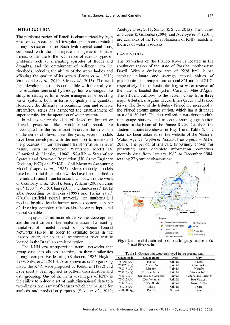
Farias, Santos, Lourenço and Carneiro
Journal of Urban and Environmental Engineering (JUEE), v.7, n.1, p.176-182, 2013
177
INTRODUCTION
The northeast region of Brazil is characterized by high rates of evaporation and irregular and intense rainfall through space and time. Such hydrological conditions, combined with the inadequate management of river basins, contribute to the occurrence of various types of problems such as alternating episodes of floods and droughts, and the entrainment of sediment into the riverbeds, reducing the ability of the water bodies and affecting the quality of its waters (Farias et al., 2010; Vanmaercke et al., 2010; Silva et al., 2013). The need for a development that is compatible with the reality of the Brazilian semiarid hydrology has encouraged the study of strategies for a better management of existing water systems, both in terms of quality and quantity. However, the difficulty in obtaining long and reliable streamflow series has hampered the establishment of superior rules for the operation of water systems.
In places where the data of flows are limited or flawed, processes like rainfall-runoff should be investigated for the reconstruction and/or the extension of the series of flows. Over the years, several models have been developed with the intention to understand the processes of rainfall-runoff transformation in river basins, such as Stanford Watershed Model IV (Crawford & Lindsley, 1966), SSARR – Streamflow Syntesis and Reservoir Regulation (US Army Engineer Division, 1972) and SMAP – Soil Moisture Accounting Model (Lopes et al., 1982). More recently, models based on artificial neural networks have been applied to the rainfall-runoff transformation, as shown in the work of Coulibaly et al. (2001), Jeong & Kim (2005), Farias et al. (2007), Wu & Chau (2011) and Santos et al. (2012 a,b). According to Haykin (1999) and Farias et al. (2010), artificial neural networks are mathematical models, inspired by the human nervous system, capable of detecting complex relationships between input and output variables.
This paper has as main objective the development and the verification of the implementation of a monthly rainfall-runoff model based on Kohonen Neural Networks (KNN) in order to estimate flows in the Piancó River, which is an intermittent river that is located in the Brazilian semiarid region.
The KNN are unsupervised neural networks that group data into classes according to their similarities through competitive learning (Kohonen, 1982; Haykin, 1999; Silva et al., 2010). Also known as self-organizing maps, the KNN were proposed by Kohonen (1982) and have mostly been applied in pattern classification and data grouping. One of the main advantages of KNN is the ability to reduce a set of multidimensional data to a two-dimensional array of features which can be used for analysis and prediction purposes (Silva et al., 2010;
Adeloye et al., 2011; Santos & Silva, 2013). The studies of Garcia & González (2004) and Adeloye et al. (2011) are examples of the few applications of KNN models in the area of water resources.
CASE STUDY
The watershed of the Piancó River is located in the southwest region of the state of Paraíba, northeastern Brazil. With a drainage area of 9228 km², it has semiarid climate and average annual values of precipitation and temperature around 821 mm and 24ºC, respectively. In this basin, the largest water reserve of the state, is located the system Coremas–Mãe d’Água. The affluent outflows to the system come from three major tributaries: Aguiar Creek, Emas Creek and Piancó River. The flows of the tributary Piancó are measured at the Piancó stream gauge station, which has a drainage area of 4170 km². The data collection was done in eight rain gauge stations and in one stream gauge station located in the basin of the Piancó River. Details of the studied stations are shown in Fig. 1 and Table 1. The data has been obtained on the website of the National Water Agency (Agência Nacional de Águas – ANA, 2010). The period of analysis, knowingly chosen for presenting more complete information, comprises monthly data from January 1963 to December 1984, totaling 22 years of observations.
Fig. 1 Location of the rain and stream studied gauge stations in the
Piancó River basin.
Table 1. Gauges that were employed in the present study Gauge code Gauge name Type City 737006 (P1) Piancó Rainfall Piancó 738020 (P2) Conceição Rainfall Conceição 738015 (P3) Manaíra Rainfall Manaíra 738013 (P4) Princesa Isabel Rainfall Princesa Isabel 738019 (P5) Santana dos Garrotes Rainfall Santana dos Garrotes 738012 (P6) Boa Ventura Rainfall Boa Ventura 738014 (P7) Nova Olinda Rainfall Nova Olinda 738018 (P8) Ibiara Rainfall Ibiara
37340000 (Q) Piancó Stream Piancó
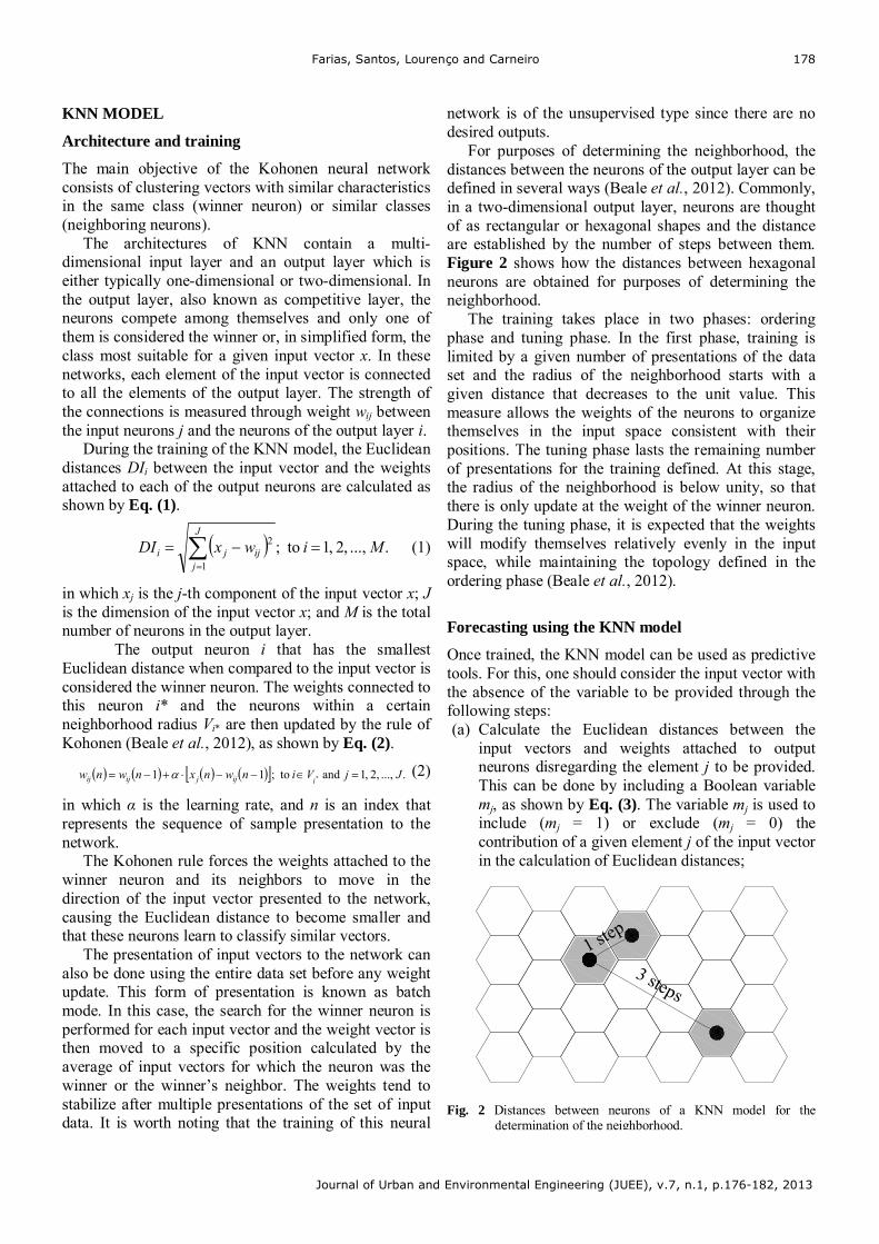
Farias, Santos, Lourenço and Carneiro
Journal of Urban and Environmental Engineering (JUEE), v.7, n.1, p.176-182, 2013
178
KNN MODEL
Architecture and training
The main objective of the Kohonen neural network consists of clustering vectors with similar characteristics in the same class (winner neuron) or similar classes (neighboring neurons).
The architectures of KNN contain a multi-dimensional input layer and an output layer which is either typically one-dimensional or two-dimensional. In the output layer, also known as competitive layer, the neurons compete among themselves and only one of them is considered the winner or, in simplified form, the class most suitable for a given input vector x. In these networks, each element of the input vector is connected to all the elements of the output layer. The strength of the connections is measured through weight wij between the input neurons j and the neurons of the output layer i.
During the training of the KNN model, the Euclidean distances DIi between the input vector and the weights attached to each of the output neurons are calculated as shown by Eq. (1).
. ..., ,2 ,1 to;1
2 MiwxDIJ
jijji
(1)
in which xj is the j-th component of the input vector x; J is the dimension of the input vector x; and M is the total number of neurons in the output layer.
The output neuron i that has the smallest Euclidean distance when compared to the input vector is considered the winner neuron. The weights connected to this neuron i* and the neurons within a certain neighborhood radius Vi* are then updated by the rule of Kohonen (Beale et al., 2012), as shown by Eq. (2).
. ..., 2, ,1 and to; 11 * JjVinwnxnwnwiijjijij (2)
in which α is the learning rate, and n is an index that represents the sequence of sample presentation to the network.
The Kohonen rule forces the weights attached to the winner neuron and its neighbors to move in the direction of the input vector presented to the network, causing the Euclidean distance to become smaller and that these neurons learn to classify similar vectors.
The presentation of input vectors to the network can also be done using the entire data set before any weight update. This form of presentation is known as batch mode. In this case, the search for the winner neuron is performed for each input vector and the weight vector is then moved to a specific position calculated by the average of input vectors for which the neuron was the winner or the winner’s neighbor. The weights tend to stabilize after multiple presentations of the set of input data. It is worth noting that the training of this neural
network is of the unsupervised type since there are no desired outputs.
For purposes of determining the neighborhood, the distances between the neurons of the output layer can be defined in several ways (Beale et al., 2012). Commonly, in a two-dimensional output layer, neurons are thought of as rectangular or hexagonal shapes and the distance are established by the number of steps between them. Figure 2 shows how the distances between hexagonal neurons are obtained for purposes of determining the neighborhood.
The training takes place in two phases: ordering phase and tuning phase. In the first phase, training is limited by a given number of presentations of the data set and the radius of the neighborhood starts with a given distance that decreases to the unit value. This measure allows the weights of the neurons to organize themselves in the input space consistent with their positions. The tuning phase lasts the remaining number of presentations for the training defined. At this stage, the radius of the neighborhood is below unity, so that there is only update at the weight of the winner neuron. During the tuning phase, it is expected that the weights will modify themselves relatively evenly in the input space, while maintaining the topology defined in the ordering phase (Beale et al., 2012).
Forecasting using the KNN model
Once trained, the KNN model can be used as predictive tools. For this, one should consider the input vector with the absence of the variable to be provided through the following steps: (a) Calculate the Euclidean distances between the
input vectors and weights attached to output neurons disregarding the element j to be provided. This can be done by including a Boolean variable mj, as shown by Eq. (3). The variable mj is used to include (mj = 1) or exclude (mj = 0) the contribution of a given element j of the input vector in the calculation of Euclidean distances;
3 steps
1 step
Fig. 2 Distances between neurons of a KNN model for the
determination of the neighborhood.
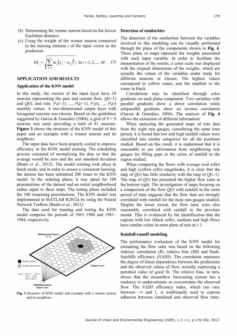
Farias, Santos, Lourenço and Carneiro
Journal of Urban and Environmental Engineering (JUEE), v.7, n.1, p.176-182, 2013
179
(b) Determining the winner neuron based on the lowest Euclidean distance;
(c) Using the weight of the winner neuron connected to the missing element j of the input vector as the prediction.
. ..., ,2 ,1 to;1
2 MiwxmDIJ
jijjji
(3)
APPLICATION AND RESULTS
Application of the KNN model
In this study, the vectors of the input layer have 18 neurons representing the past and current flow, Q(t–1) and Q(t), and rain, P1(t–1), ..., P8(t–1), P1(t), ..., P8(t) monthly values. A two-dimensional output layer with hexagonal neurons was chosen. Based on the guidelines suggested by Garcia & González (2004), a grid of 9 × 9 neurons was used, providing a total of 81 neurons. Figure 3 shows the structure of the KNN model of this paper and an example with a winner neuron and its neighbors.
The input data have been properly scaled to improve efficiency in the KNN model training. The scheduling process consisted of normalizing the data so that the average would be zero and the unit standard deviation (Beale et al., 2012). The model training took place in batch mode, and in order to ensure a consistent learning, the dataset has been submitted 200 times to the KNN model. In the ordering phase, it was opted for 100 presentations of the dataset and an initial neighborhood radius equal to three steps. The tuning phase included the 100 remaining presentations. The KNN model was implemented in MATLAB R2012a by using the Neural Network Toolbox (Beale et al., 2012).
The data used for training and testing the KNN model comprise the periods of 1963–1980 and 1981–1984, respectively.
Fig. 3 Structure of KNN model and example with a winner neuron
and its neighbors.
Detection of similarities
The detection of the similarities between the variables involved in this modeling can be visually performed through the plans of the components shown in Fig. 4. Those plans or maps represent the weights associated with each input variable. In order to facilitate the interpretation of the results, a color scale was displayed with the original dimensions of the weights, which are actually the values of the variables under study for different neurons or classes. The highest values correspond to yellow zones, and the smallest to the zones in black.
Correlations may be identified through color gradients on each plane component. Two variables with parallel gradients show a direct correlation while antiparallel gradients show an inverse correlation (Garcia & González, 2004). The analysis of Fig. 4 allows the extraction of different information.
When analyzing the generated maps of rain data from the eight rain gauges, considering the same time period, it is found that low and high rainfall values were classified into similar categories for all the positions studied. Based on this result, it is understood that it is reasonable to use information from neighboring rain gauges for filling gaps in the series of rainfall in the region studied.
When comparing the flows with average (red cells) and high (yellow cells) magnitudes, it is clear that the map of Q(t) has little similarity with the map of Q(t–1). The map of Q(t) has presented the higher flow rates at the bottom right. The investigation of maps focusing on a comparison of the flow Q(t) with rainfall in the same period of time suggests that the flow data are strongly correlated with rainfall for the most rain gauges studied. Despite the lesser extent, the flow rates were also reasonably correlated with rainfall in the previous month. This is evidenced by the identification that the regions with low (black cells), medium and high flows have similar colors in most plans of rain at t–1.
Rainfall-runoff modeling
The performance evaluation of the KNN model for estimating the flow rates was based on the following indexes: correlation (R), relative bias (RB) and Nash-Sutcliffe efficiency (NASH). The correlation measures the degree of linear dependence between the predictions and the observed values of flow, actually expressing a potential value of good fit. The relative bias, in turn, shows that the streamflow forecasting system has a tendency to underestimate or overestimate the observed flow. The NASH efficiency index, which can vary between –∞ and 1, is traditionally used to express adhesion between simulated and observed flow rates.
1
2
81
Vector = [P(t-1), ... , P(t-1), P(t), ... , P(t), Q(t-1); Q(t) ]
9
11
12
18
73
74
1 8
1 8
Bidimensional Space9 × 9
MultidimensionalInput Layer
Output Layer
Winning neuron
Neighboring neurons
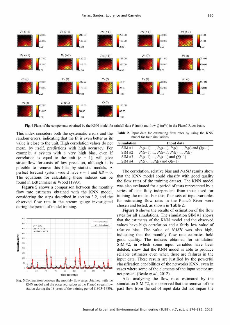
Farias, Santos, Lourenço and Carneiro
Journal of Urban and Environmental Engineering (JUEE), v.7, n.1, p.176-182, 2013
180
This index considers both the systematic errors and the random errors, indicating that the fit is even better as its value is close to the unit. High correlation values do not mean, by itself, predictions with high accuracy. For example, a system with a very high bias, even if correlation is equal to the unit (r = 1), will give streamflow forecasts of low precision, although it is possible to remove this bias by statistic models. A perfect forecast system would have r = 1 and RB = 0. The equations for calculating these indexes can be found in Lettenmaier & Wood (1993).
Figure 5 shows a comparison between the monthly flow rate estimates obtained with the KNN model, considering the steps described in section 3.2, and the observed flow rate in the stream gauge investigated during the period of model training.
Fig. 5 Comparison between the monthly flow rates obtained with the
KNN model and the observed values at the Piancó streamflow station during the 18 years of the training period (1963–1980).
Table 2. Input data for estimating flow rates by using the KNN model for four simulations
Simulation Input data SIM #1 P1(t–1), ..., P8(t–1), P1(t), ..., P8(t) and Q(t–1) SIM #2 P1(t–1), ..., P8(t–1), P1(t), ..., P8(t) SIM #3 P1(t–1), ..., P8(t–1) and Q(t–1) SIM #4 P1(t), ..., P8(t) and Q(t–1)
The correlation, relative bias and NASH results show
that the KNN model could classify with good quality the flow rates of the training dataset. The KNN model was also evaluated for a period of tests represented by a series of data fully independent from those used for training the model. For this, four sets of input variables for estimating flow rates in the Piancó River were chosen and tested, as shown in Table 2.
Figure 6 shows the results of estimation of the flow rates for all simulations. The simulation SIM #1 shows that the estimates of the KNN model and the observed values have high correlation and a fairly low value of relative bias. The value of NASH was also high, indicating that the monthly flow rate estimates hold good quality. The indexes obtained for simulation SIM #2, in which some input variables have been deleted, show that the KNN model is able to produce reliable estimates even when there are failures in the input data. These results are justified by the powerful classification capabilities of the networks KNN, even in cases where some of the elements of the input vector are not present (Beale et al., 2012).
Also analyzing the flow rates estimated by the simulation SIM #2, it is observed that the removal of the past flow from the set of input data did not impair the
0
50
100
150
200
250
300
350
400
450
500
1 25 49 73 97 121 145 169 193
Time (months)
Stre
amfl
ow (
m³/
s)
Observed
Calculated r = 0.90 RB = -0.15 NASH = 0.75
Fig. 4 Plans of the components obtained by the KNN model for rainfall data P (mm) and flow Q (m³/s) in the Piancó River basin.
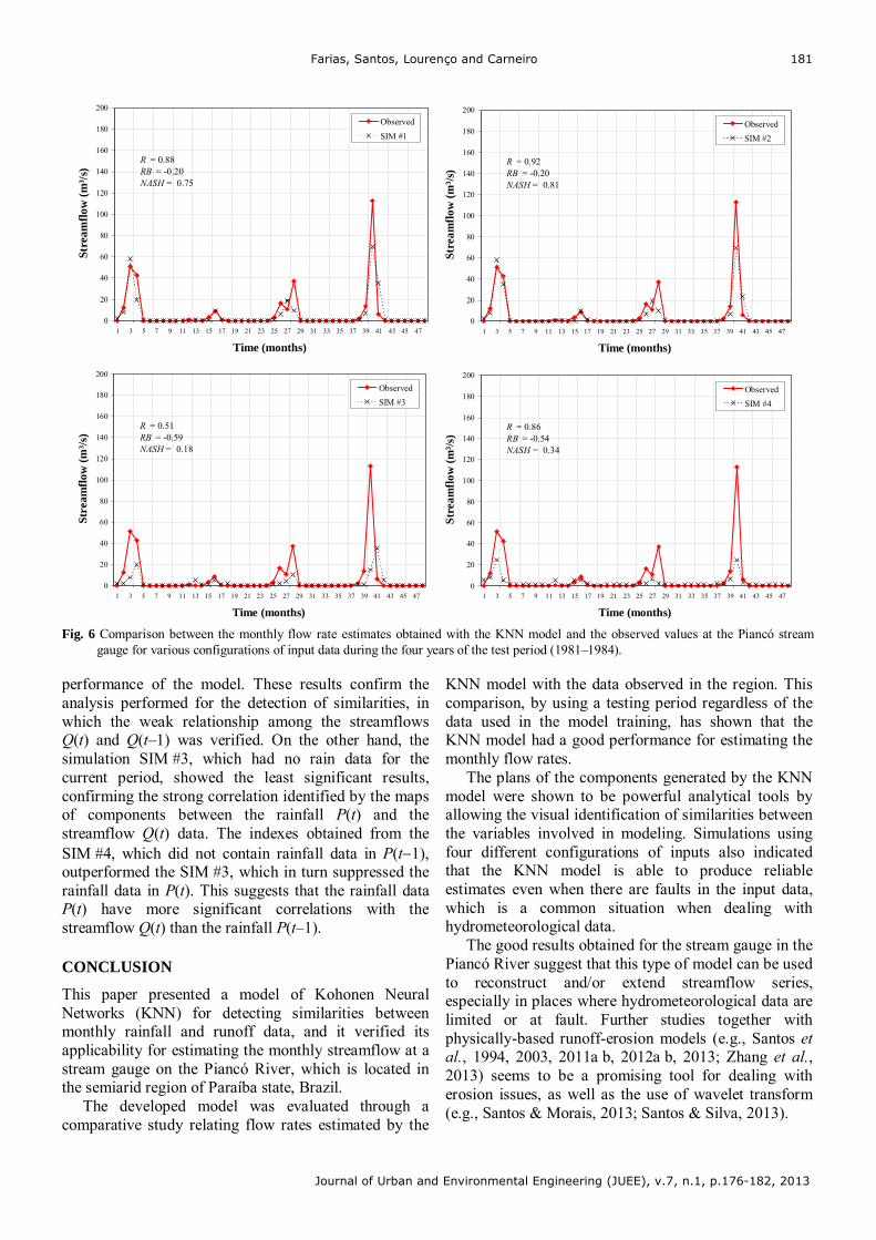
Farias, Santos, Lourenço and Carneiro
Journal of Urban and Environmental Engineering (JUEE), v.7, n.1, p.176-182, 2013
181
performance of the model. These results confirm the analysis performed for the detection of similarities, in which the weak relationship among the streamflows Q(t) and Q(t–1) was verified. On the other hand, the simulation SIM #3, which had no rain data for the current period, showed the least significant results, confirming the strong correlation identified by the maps of components between the rainfall P(t) and the streamflow Q(t) data. The indexes obtained from the SIM #4, which did not contain rainfall data in P(t1), outperformed the SIM #3, which in turn suppressed the rainfall data in P(t). This suggests that the rainfall data P(t) have more significant correlations with the streamflow Q(t) than the rainfall P(t–1). CONCLUSION
This paper presented a model of Kohonen Neural Networks (KNN) for detecting similarities between monthly rainfall and runoff data, and it verified its applicability for estimating the monthly streamflow at a stream gauge on the Piancó River, which is located in the semiarid region of Paraíba state, Brazil.
The developed model was evaluated through a comparative study relating flow rates estimated by the
KNN model with the data observed in the region. This comparison, by using a testing period regardless of the data used in the model training, has shown that the KNN model had a good performance for estimating the monthly flow rates.
The plans of the components generated by the KNN model were shown to be powerful analytical tools by allowing the visual identification of similarities between the variables involved in modeling. Simulations using four different configurations of inputs also indicated that the KNN model is able to produce reliable estimates even when there are faults in the input data, which is a common situation when dealing with hydrometeorological data.
The good results obtained for the stream gauge in the Piancó River suggest that this type of model can be used to reconstruct and/or extend streamflow series, especially in places where hydrometeorological data are limited or at fault. Further studies together with physically-based runoff-erosion models (e.g., Santos et al., 1994, 2003, 2011a b, 2012a b, 2013; Zhang et al., 2013) seems to be a promising tool for dealing with erosion issues, as well as the use of wavelet transform (e.g., Santos & Morais, 2013; Santos & Silva, 2013).
0
20
40
60
80
100
120
140
160
180
200
1 3 5 7 9 11 13 15 17 19 21 23 25 27 29 31 33 35 37 39 41 43 45 47
Time (months)
Stre
amfl
ow (
m³/
s)
Observed
SIM #1
R = 0.88 RB = -0.20 NASH = 0.75
0
20
40
60
80
100
120
140
160
180
200
1 3 5 7 9 11 13 15 17 19 21 23 25 27 29 31 33 35 37 39 41 43 45 47
Time (months)
Stre
amfl
ow (
m³/
s)
Observed
SIM #2
R = 0.92 RB = -0.20 NASH = 0.81
0
20
40
60
80
100
120
140
160
180
200
1 3 5 7 9 11 13 15 17 19 21 23 25 27 29 31 33 35 37 39 41 43 45 47
Time (months)
Stre
amfl
ow (
m³/
s)
Observed
SIM #3
R = 0.51 RB = -0.59 NASH = 0.18
0
20
40
60
80
100
120
140
160
180
200
1 3 5 7 9 11 13 15 17 19 21 23 25 27 29 31 33 35 37 39 41 43 45 47
Time (months)
Str
eam
flow
(m
³/s)
Observed
SIM #4
R = 0.86 RB = -0.54 NASH = 0.34
Fig. 6 Comparison between the monthly flow rate estimates obtained with the KNN model and the observed values at the Piancó stream
gauge for various configurations of input data during the four years of the test period (1981–1984).
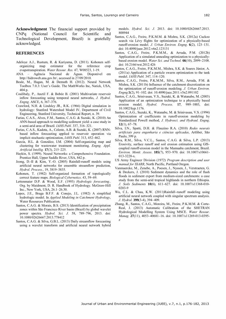
Farias, Santos, Lourenço and Carneiro
Journal of Urban and Environmental Engineering (JUEE), v.7, n.1, p.176-182, 2013
182
Acknowledgment The financial support provided by CNPq (National Council for Scientific and Technological Development, Brazil) is gratefully acknowledged. REFERENCES
Adeloye A.J., Rustum, R. & Kariyama, D. (2011). Kohonen self-organizing map estimator for the reference crop evapotranspiration. Water Resour. Res. 47, W08523, 1-19.
ANA – Agência Nacional de Águas. Disponível em http://hidroweb.ana.gov.br/, accessed in 27/09/2010.
Beale, M., Hagan, M. & Demuth H. (2012). Neural Network Toolbox 7.0.3: User’s Guide. The MathWorks Inc, Natick, USA, 404 p.
Coulibaly, P., Anctil F. & Bobée B. (2001) Multivariate reservoir inflow forecasting using temporal neural networks, J. Hydrol. Engng. ASCE, 6, 367–376.
Crawford, N.H. & Lindsley JR., R.K. (1966) Digital simulation in hydrology: Stanford Watershed Model IV, Department of Civil Engineering, Stanford University, Technical Report, n. 39.
Farias, C.A.S., Alves, F.M., Santos, C.A.G. & Suzuki, K. (2010) An ANN-based approach to modelling sediment yield: a case study in a semi-arid area of Brazil. IAHS Publ. 337, 316–321.
Farias, C.A.S., Kadota, A., Celeste, A.B. & Suzuki, K. (2007) RNN-based inflow forecasting applied to reservoir operation via implicit stochastic optimization, IAHS Publ. 313, 452–462.
García, H.L. & González, I.M. (2004) Self-organizing map and clustering for wastewater treatment monitoring. Engng. Appl. Artificial Intellig. 17(3), 215–225.
Haykin, S. (1999). Neural Networks: a Comprehensive Foundation. Prentice Hall, Upper Saddle River, USA, 842 p.
Jeong, D.-II & Kim, Y.-O. (2005) Rainfall-runoff models using artificial neural networks for ensemble streamflow prediction, Hydrol. Process., 19, 3819–3835.
Kohonen, T. (1982) Self-organized formation of topologically correct feature maps. Biological Cybernetics. 43, 5969.
Lettenmaier D.P. & Wood, E.F. (1993) Hydrologic forecasting.. Org. by Maidment, D. R. Handbook of Hydrology. McGraw-Hill Inc., New York, USA, 26.1–26.30.
Lopes, J.E., Braga B.F.F. & Conejo, J.L. (1982) A simplified hydrologic model. In Applied Modeling in Catchment Hydrology, Water Resources Publication.
Santos, C.A.G. & Morais, B.S. (2013) Identification of precipitation zones within São Francisco River basin (Brazil) by global wavelet power spectra. Hydrol. Sci. J. 58, 789–796, 2013. doi: 10.1080/02626667.2013.778412
Santos, C.A.G. & Silva, G.B.L. (2013) Daily streamflow forecasting using a wavelet transform and artificial neural network hybrid
models. Hydrol. Sci. J. 2013. doi: 10.1080/02626667.2013. 800944
Santos, C.A.G., Freire, P.K.M.M. & Mishra, S.K. (2012a) Cuckoo search via Lévy flights for optimization of a physically-based runoff-erosion model. J. Urban Environ. Engng. 6(2), 123–131. doi: 10.4090/juee.2012.v6n2.123131
Santos, C.A.G., Freire, P.K.M.M., & Arruda, P.M. (2012b) Application of a simulated annealing optimization to a physically-based erosion model. Water Sci. and Technol. 66(10), 20992108. doi: 10.2166/wst.2012.426
Santos, C.A.G., Freire, P.K.M.M., Mishra, S.K. & Soares Júnior, A. (2011a) Application of a particle swarm optimization to the tank model. IAHS Publ. 347, 114–120.
Santos, C.A.G., Freire, P.K.M.M., Silva, R.M., Arruda, P.M. & Mishra, S.K. (2011b) Influence of the catchment discretization on the optimization of runoff-erosion modeling. J. Urban Environ. Engng.5(2), 91–102. doi: 10.4090/juee.2011.v5n2.091102
Santos, C.A.G., Srinivasan, V.S., Suzuki, K. & Watanabe, M. (2003) Application of an optimization technique to a physically based erosion model. Hydrol. Process. 17, 989–1003, doi: 10.1002/hyp.1176.
Santos, C.A.G., Suzuki, K., Watanabe, M. & Srinivasan, V.S. (1994) Optimization of coefficients in runoff-erosion modeling by Standardized Powell method, J. Hydrosci. and Hydraul. Engng. 12(1), 67–78.
Silva, I.N., Spatti, D.H. & Flauzino R.A. (2010) Redes neurais artificiais para engenharia e ciências aplicadas, Artliber, São Paulo, 399 p.
Silva, R.M., Silva, V.C.L., Santos, C.A.G. & Silva, L.P. (2013) Erosivity, surface runoff and soil erosion estimation using GIS-coupled runoff-erosion model in the Mamuaba catchment, Brazil. Environ. Monit. Assess. 185(7), 953–970. doi: 10.1007/s10661-013-3228-x.
US Army Engineer Division (1972) Program description and user manual for SSARR, North Pacific, Portland Oregon.
Vanmaercke, M., Zenebe, A., Poesen, J., Nyssen, J., Verstraeten, G. & Deckers, J. (2010) Sediment dynamics and the role of flash floods in sediment export from medium-sized catchments: a case study from the semi-arid tropical highlands in northern Ethiopia. J. Soils Sediments 10(6), 611–627. doi: 10.1007/s11368-010-0203-9
Wu, C.L. & Chau, K.W. (2011)Rainfall–runoff modeling using artificial neural network coupled with singular spectrum analysis. J. Hydrol. 399(3-4), 394409.
Zhang, R., Santos, C.A.G., Moreira, M., Freire, P.K.M.M. & Corte-Real, J. (2013) Automatic Calibration of the SHETRAN Hydrological Modelling System Using MSCE. Water Resour. Manag. 27(11), 4053–40681–16. doi: 10.1007/s11269-013-0395-z
Journal of Urban and Environmental Engineering (JUEE), v.7, n.1 p.183-194, 2013
Journal of Urban and Environmental Engineering, v.7, n.1 p. 183-194, 2013
Journal of Urban and Environmental Engineering
UEEJ ISSN 1982-3932
doi: 10.4090/juee.2013.v7n1.183194 www.journal-uee.org
AN ANALYSIS OF REGIONAL DISPARITIES SITUATION IN THE EAST AZARBAIJAN PROVINCE
Nader Zali1, Hassan Ahmadi2 and Seyed Mohammadreza Faroughi3
1 Assistant Professor, Department of Urban Planning, University of Guilan, Iran 2 Assistant Professor, Department of Urban Planning, University of Guilan, Iran
3 Department of Urban Planning, University of Guilan, Iran
Abstract: The regional disparity in Iran is now a matter of serious concern. Measuring
development has been a matter of debate for nearly half a century. The conventional way of assessing development by social and economic indicators only has been challenged many times during this period. Accelerated urbanization in developing countries and the concentration of activities and population in some regions, have led to regional imbalances. This is one of the important characteristics of the third world countries. This characteristics is affected by pole growth policies that have led to a concentration of facilities in one or more of several regions. In this case, regional planning science offers beneficial patterns to resolve problems. The first step is the identification of socio-economical disparities in these regions. However, this article attempts to survey development disparities in the East Azarbaijan province. In this survey 44 indicators were selected for the comparison of the counties, and the Numeric Taxonomic & Cluster Analysis methods were used to rank the regions. Finally this article presents priority of counties for investment in order to achieve social justice. According to the results of this research the west area of the province is prosperous and east area has a low degree of development.
Keywords:
Development Ranking, Foresight, Regional Disparities, East Azarbaijan
© 2013 Journal of Urban and Environmental Engineering (JUEE). All rights reserved.
Correspondence to: Nader zali, Tel.: +98 914 303 8588. E-mail: [email protected]
Zali, Ahmadi and Faroughi
Journal of Urban and Environmental Engineering (JUEE), v.7, n.1 p.183-194, 2013
184
INTRODUCTION In general, disparities between regions and inside them occur as result of some concentration, agglomeration, trends triggered by external phenomena, globalization, integration, or by internal ones, clustering, emergence of growth/development poles, involvement of local institutions in various aspects of economic life, etc. As a rule, regional disparities take the shape of differences between the level of incomes per capita and determine, at a given moment, a chain reaction of companies, authorities, inhabitants, etc., that attempt to counteract their escalation (Antonescu, 2012)
One of the characteristics for third world countries is a high concentration of population and activities, and space disparity in the enjoyment of social conveniences. This was found before the Revolution in Iran and in its effects after the Revolution in Iran. Based on this tendency, a main portion of facilities and the population concentrate in one or more places. Other regions act as boundaries resulting in regional disparities.
Regional disparities derive from two main fields: first the natural conditions in any geographical region and second the economical plan & policy makers' decisions. It should ne mentioned that the first factor declines with technological development and the second factor is considered to be more important. The plan & policy makers' decisions play the most important role in creating regional disparity.
PROBLEM VIEW Inequality and its different dimensions are the significant signs of underdevelopment. Regional inequalities represent a continuing development challenge in most countries, especially those with large geographic areas under their jurisdictions. Large regional disparities represent serious threats to countries as they create potential for disunity and, in extreme cases, for disintegration. Marginalized populations often are left excluded when important development and investment decisions are made. Regional disparities in Iran have been growing at an alarming rate leading to serious problems including migration with its associated problems from backward provinces to the more affluent ones. So that, the Human Development Report for Iran in 1999 reflected such disparities and reiterated that one of the major human development policies in the country’s Third Plan is to “pay attention to the spatial planning as a long-term framework for social justice and regional balance”. In order to provide a scientific basis to decrease regional inequalities, it is very necessary to comprehensively assess the status of regional development with regard to different indicators. Once this assessment is done and we get a clear idea of the backwardness of some regions, we can proceed to tackle the problems of backward regions. The aim of this study
is to assessment the regional development inequalities in Iran at sub-province scale. In this way, multi criteria decision making methods were applied for evaluating regional development level of sub-provinces (Tagvaei, 2012).
Plan and policy makers propose the necessity for equal development for different reasons: first, to establish social equality in order to be enjoyed of facilities in equality and appropriate for many reasons. Second, political considerations serve as a parameter to decrease political unrests and third, social and economical considerations prevent immigration and over-concentration of people. Based on this, the Islamic Republic of Iran's constitute enforces the government to structure for a correct and fair economy to regulate justice-based economical plans in order to establish welfare, resolve poverty, eliminate deprivation and establish social justice.
It seems that despite executing some development plans for Azerbaijan, the Sharghi province's development, it is still remained subject to inequality and disparity in terms of facility distribution. Unequal distribution of facilities inevitably result from a high density of the population, activities and services in some regions, incompatible with the weight of population, activities and services in other regions that results in an increasing population flow so that officials face with considerable problems. This phenomenon causes current economical life of small towns and villages’ in these regions to be inactivated, with increasingly mobile small cities' population and incapability to restrain big cities' population growth.
It is natural that the above-mentioned increase of centralization results in a wide variety of problems in the performance phase for managers and decision-makers. Based on this, it seems that no plan would be able to address this disparity or restrict its intensification unless it considered the suitable distribution of social facilities and services (Zali, 2000).
In this direction, the consideration of regional disparities based on indices is supposed to be one of the most important planning tools by which plan makers can assess the results of a plan’s execution in the context of geographical boundaries. If considered by plan makers logically and scientifically, such considerations can clearly reveal the strengths and weaknesses of planning in various areas and determine planning regions in aspect of enjoyment scale based on hierarchy and homogeneity of regions (Zali, 2000). The distribution of services and facilities can be evaluated through a comparative examination of various skeletal, social and economical indices in different regions. Indices compare the status of various geographical regions, prioritizing them based on the quality of their facilities and general conditions. In this way, we may be able to propose the capabilities and conditions of various geographical scopes in terms of theor enjoyment
Zali, Ahmadi and Faroughi
Journal of Urban and Environmental Engineering (JUEE), v.7, n.1 p.183-194, 2013
185
of services, infrastructures, etc. and to provide the necessary tools for decision-making and other objective determinations.
This paper examines the Azrbaijan Sharghi counties’ access to social services and facilities, by compiling different indices and measurements in social, production, and infrastructural fields, and examining how facilities are distributed. The information can then be used to formulate the plans and specific objectives to achieve social equality and reduce regional disparity. REGIONAL INEQUALITY THEORETICAL ARGUMENTS The interaction of inequality and growth has been a topic with several questions but without clear answers. On the one hand, it is asked whether inequality is good or bad for growth. On the other hand, the question is whether growth increases or reduces inequalities. Thus, not only the direction of the relationship (positive or negative), but also the direction of causality is of interest. None of those questions has been answered unanimously in the theoretical and empirical literature.(Paas, 2009)
The literature on inequality and growth considers usually the effects of individual inequality to economic growth (an overview is Kanbur, 2000). There are a lot of empirical investigations (e.g. Barro, 2000; Forbes, 2000), delivering contradictory results. For example, Barro (2000) obtains only a weak relationship between income inequality and growth. He argues that this is consistent with the mixed theoretical arguments: the forces working in opposite directions cancel out each other.
The theories touching most directly on regional inequality and economic growth are trade and growth theories, considering also the persistence of regional inequalities. The most well known arguments for decreasing regional inequalities come from the neoclassical approach. In the neoclassical world with free trade or free movement of production factors and perfect competition, regional inequalities should vanish. The production factors are paid according to their marginal products and these would equalise over the space as the firms look for the location with lowest production costs. However, if regions are characterised by differences
in technological level or other factors that influence the productivity of the production factors, the inequalities may be persistent.
The neoclassical arguments for vanishing inequalities between nations or regions have been the basis for the convergence literature (e.g. Barro, 1991). The full equalisation of the prices of the production factors is captured by the concept of absolute convergence. In case of technological differences each region or country converges towards its own steady state, denoted by conditional convergence (Barro & Sala-i-Martin, 1995).
These convergence concepts are in line with the classical trade theory (Feenstra, 2004). The arguments for absolute convergence rely usually on the Solow growth model (Solow, 1956) which predicts the long run growth rate to approach the rate of technological progress in the long run. In fact, this model was rather constructed for analysing the growth path of one country than comparing the speed of growth across spatial units (Solow, 2001). Conditional convergence is consistent with endogenous growth models (Romer, 1986, 1990; Lucas, 1988) in which technological progress is modelled as depending on the contributions to the research and development sector.
Another group of models discussing the interaction of regional inequality and growth belongs to the field of new economic geography (NEG) models (Baldwin et al., 2003). These models are characterised by increasing returns to scale in production, monopolistic competition, costly interregional trade and factor mobility. In the first paper of the field, Krugman (1991) showed that regional inequalities might be persistent because of the so called home market effect: it is beneficial to locate production close to a large market as this enables to increase sales and profits. As splitting production between several regions is not profitable due to increasing returns to scale, each firm produces only in one region. Costly trade causes the prices of the products to be higher in regions that are served by exporting and, thus, the firms are able to sell smaller quantities of their products there than in the home region. Moreover, the low prices carry over to high real wages that attract mobile workers to the region with more firms. The wages are additionally drawn up in that region due to the competition of the firms for workers. The home market effect appears also if the workers are assumed to be immobile, but the products of the firms are used by other firms as intermediate inputs (Krugman and Venables, 1995).
Zali, Ahmadi and Faroughi
Journal of Urban and Environmental Engineering (JUEE), v.7, n.1 p.183-194, 2013
186
As the result, in a two region setting the firms and workers concentrate in one of the regions (the core) if the trade costs are sufficiently low even if the regions are initially identical in their technological level and resource endowments. In fact, the home market effect was already present in Krugman’s (1980) trade model without labour mobility. However, that model was unable to explain the emergence of agglomerations of economic activity in case of symmetric regions, i.e. the inequalities that can be observed in space. (Paas, 2009)
Some further developments in the field have directly tackled the interplay of growth and regional inequality. The first paper to address this question was Baldwin (1999). Abstracting from factor mobility, he shows that growth can affect inequality. This is achieved by the assumption that capital (utilised by the modern sector) depreciates and has to be replaced. Also, investment into capital construction will be done only if the present value of its expected flow of return is at least as large as the investment costs. Another assumption is that the constructed capital can be utilised for producing the consumer goods only in the region of construction.
The spatial equilibrium is achieved if the expected return from capital covers exactly its construction costs: in that case there will be no growth. However, if from one of the initially identical regions one modern firm decides to relocate to the other region and the trade costs are sufficiently low, there starts a growth process in the now larger region and economic contraction process in the smaller region. The reason behind this result is again the home market effect, enabling the firms in the larger region to earn higher profits than before the relocation, and vice versa in the now smaller region. Construction of capital is then unprofitable in the smaller region as the firms are not able to earn sufficiently high profits to cover the capital construction costs. Thus, the initially small inequality increases gradually. If the two regions of the economy were initially identical, this agglomeration process lasts until the whole modern sector has concentrated into the larger region. If the regions are initially of different size, also partial agglomeration is possible, but in case of very low trade costs still full agglomeration occurs.
Such an agglomeration process can occur only if capital is immobile. Clearly, there are almost no mobility restrictions to the flows of monetary capital in the nowadays world. However, it is
difficult or impossible to move machines and buildings necessary for production. Thus, this crucial assumption of the model is not overly unrealistic.
In this constructed capital model growth and inequality interact in both directions: inequality has growth effects (increases the disparities in the growth rates of the regions) and growth in one and recession in the other region increases of course regional inequality. Thus, differently from the neoclassical growth theory in this model the richer region grows faster as also described by Myrdal (1957) with the concept of cumulative causation. However, once full agglomeration in the core has been achieved, its growth comes to a halt. If now liberalisation of trade continues, there will be gradual growth in terms of real income in the other, peripheral region. The reason behind this result is a decrease in prices as less has to be paid for transporting the goods from the core region. Still, even when trade is fully liberalised, there remain differences in the per capita incomes across the two regions though not as high as for a medium range of trade costs. However, if capital mobility is allowed, these effects vanish and convergence is achieved. Considering the whole economy’s income per capita, the degree of regional inequality has according to the model no effect in the long run if trade costs do not change. (Paas, 2009).
Also endogenous growth models have been developed in the context of the NEG. In these models the degree of inequality has also consequences for national growth. The most well known endogenous NEG model is due to Martin and Ottaviano (1999), the spillovers model. Their model is an upgrade of the constructed capital model. For achieving endogeneity of growth, they assume spillovers in the capital construction sector: the more capital there is in the economy, the cheaper it is to construct new capital (global spillovers). It can also be assumed that the spillovers from the other region are not captured as easily as those from the home region, i.e. the local capital stock has a larger impact on the innovation efficiency (local spillovers). The conclusions from the spillovers models coincide largely with those from the constructed capital model (Baldwin et al. 2003), but give also new insights to the interplay of regional inequality and growth.
Differently from the constructed capital model there is a continuous growth in the national real per capita income also in the long run equilibrium.
Zali, Ahmadi and Faroughi
Journal of Urban and Environmental Engineering (JUEE), v.7, n.1 p.183-194, 2013
187
However, as in the constructed capital model the income levels differ if the capital stock and modern sector firms are distributed unevenly in the space, also in case of completely free trade. The most important result reveals that the national growth rate is highest if the capital construction activity and thus, the production of the increasing returns goods are present only in one region given that the spillovers have local character and trade costs are sufficiently low. Moreover, if the share of the modern goods is sufficiently high in the consumption expenditures, the welfare level is higher in the peripheral region than it would be under a symmetric distribution of firms. Once again, if gradual liberalisation of trade takes place, the relative real incomes of the two regions change similarly to those in the constructed capital model.
The above introduction of the NEG models support positive correlation between regional inequality and the speed of economic growth. However, the models have some drawbacks, that might influence the outcomes of testing this conclusion empirically. First, the models are constructed for a two region economy, but in the reality countries consist of several regions and have interactions with regions from other countries.
However, it has been shown for the simple NEG models that the occurrence of agglomerations of economic activity holds also in multiregional context (Fujita et al., 1999). For the interaction with a foreign region, Krugman and Livas Elizondo (1996) have shown that integration with a region from abroad motivates a relocation within the home economy towards the border, especially if the foreign region has a large market.
The second issue considers the negligence of congestion cost. If lots of economic activity concentrates in just one region, the housing and land prices are driven up, there can occur environmental problems and the loss of efficiency due to e.g. traffic jams. Adding such aspects to the model would motivate the firms to move out of the core regions, as shown for example by Helpman (1998).
Finally Economic theorists have proposed many ideas to revive structural development. Some, like Rosenstein Rodan and Narks have found that the simultaneous growth of economic sectors is necessary in order to achieve economic development. They believe multilateral and simultaneous investment in various economic sectors is necessary in order to beak the debilitating cycle of poverty in developing countries. This is the balanced growth theory. In contrast,
Hirschman believes that developing countries do not possess enough capital to be able to perform such multilateral investments. These countries have to choose an area of focus in which to invest and thus pioneer development by establishing a growth pole until the growth rate of this area causes the growth of other areas (Beheshti, 1983).
There are probably identical methods over regions development. The concept of a growth pole was proposed by François Pro (French) in the 1960s. He believed that growth poles would include some industries and high-functioning factories with a high growth rate. He identified that the advanced and basic industrial growth was an engine for the growth of the national economy, and that imbalanced growth would occur. New industries would inevitably be settled on neighboring infrastructures, stimulating certain growth points. Such centralization would encourage backwardness of other regions and result in geographically regional polarization and heterogeneous development. Several seminal works will ensure the correction of the imbalance (Harvy, 1997). It is possible to detect those regions being far away from social equality standards via this method (Hakimi, 1992).
It is his belief, that if development is not accompanied with a coherent social policy that directly addresses the reasons for poverty and under-development, it will be impossible to attain a solution that will address the poverty and disparity in the various regions and communities. Regional development follows three objectives: productivity, society and biology. Regional development attempts to provide the best condition and facilities for comprehensive development, minimize life quality differences between regional and inter-regional and finally resolve it (Mokhber, 1988).
In late 70s and early 80s, concern about increasingly economical disparities in the third world resulted in new approaches toward development policy that focused on resolving basic needs. These approaches derived from a concern that even redistribution policies associated with growth would not be able to improve the welfare of the poorest classes of the society. In the 1980s, neoclassic theorists established neoclassic reciprocal revolution theory. This notion focused more on privatization and less on governmental interference, and emphasized a belief in the free market. Such theories advanced the ideas that disappointment in development gains originates from excessive government interference in economic affairs (Ardeshiri, 2000).
Accordingly, a new theory of growth was outlined based on innate growth and constant development in this decade. Constant development is being followed seriously in the recent years, meaning not only preservation of environment but the new concept of economic growth which offers life facility and equality for all people in the world, not just for a few people.
Zali, Ahmadi and Faroughi
Journal of Urban and Environmental Engineering (JUEE), v.7, n.1 p.183-194, 2013
188
METHODOLOGY Comparing geographical regions based on one or more development index value might be possible in two ways: first, instance comparison, i.e. to determine the development scale of each region based on any index that is neither logical nor actually represents development scale in each region. Second, through a general comparison and selection of those indices that represent the development symptoms of the region we specify a quantity from the indices scientific aggregation, and classify regions according to this quantity. It seems that the second method is especially suitable to detect quality of life statuses. It is essential to use statistical and analytical models to gauge and compare these figures, by compiling a number of indices to obtain the status of any region against other regions. There are several scientific methods in this field including: Numeric taxonomy, factor analysis, deprivation coefficient, cluster analysis, the Murris method and the sum of standard data method.
Among these, the numeric taxonomy method is considered to be one of the most current methods for classification, well-regarded most by plan makers in recent years. Nevertheless, this technique is not free from limitation. For instance, it does not encourage the translation of indices into analysis and classification. Those indices that usually define each other locate together, probably boosting each other to manipulate the results of analysis. According to experts, despite such defects, it is more reliable to use the numeric taxonomy technique rather than any of the other techniques mentioned above.
Taxonomy as a general name refers to those methods that separate similar cases from dissimilar ones. One of the most important is numeric taxonomy which is capable both of classifying a series as a scale and of identifying the under-development status of regions (Borzooyan, 1995). Taxonomy is regarded as a statistical method to specify units or any homogeneous types into a latter N diagram space without the use of variance regression or correlation analysis (Bidabad, 1983).
This method was first offered by Adanson in 1984, and proposed by Prof. Zygmunt Hellwing from Rekla economy premier college in UNESCO as a tool for the classification of the under-development scale between various nations. This method is considered as a premier method for the rating, classification and comparison of countries of different regions, regarding their development scale. In the taxonomy method, the indices maximum quantity is chosen as the target quantity for the region’s rating after indices harmonization and standardization, and measuring the distance of other resources with the target index. Those regions showing less distance from the intended target will be regarded as more developed regions. The taxonomy output will
show as a quantity called Fi that represents the deprivation scale for any region ranging from zero to one, so that the higher the index, the higher the deprivation on this scale.
The scale is arrived at by the cluster analysis method to determine the homogeneous groups after rating. This method divides counties based on their distance from the intended target with other counties in the same homogeneous classes. Under this method, the quantitative properties of the counties of each group possess relative and close similarities toward one another. SELESTION AND CLASSIFICATION OF INDIXES In this study 44 indices among several indices as counties enjoyment scale were chosen, regarded as a base to rank counties in several regions. Among these, there were 8 basic indices,8 production indices, 15 social indices and 13 infrastructure indices which wholly listed separately as below: BASIC INDIXED
Employment rate, family density, municipalities' per capita income, per capita tax, the number of bank branches as for 10,000 people, high educated employed percentage, population density, urbanism percentage. PRODUCTION INDIXES
Cultivated area for each beneficiary, consumptive water coefficient in production section to total electric consumption, one hectare garden products turnover per hectare, cultivation products turnover per hectare, utilization ratio of agricultural instruments per every 10 hectare of agricultural field, the ratio of large industrial workshop workers per total workers, the number of industrial active and cooperative co. workers per 100,000 people SOCIAL INDIXES
Literacy rate, student ratio to training cadre, sport fields area per capita, public library books per capita, cinema capacity, number of printing office, number of nurseries, number of students, number of health care and treatment centers, number of hospital beds, general practitioners, dentists, number with access to heath care and birth control centers per 100,000 people. INFRASTRUCTURE INDIXES
The asphalted village road ratio to total village roads, the number of working cable phones, cell phones, the percentage of households with gas pipes, villages
Zali, Ahmadi and Faroughi
Journal of Urban and Environmental Engineering (JUEE), v.7, n.1 p.183-194, 2013
189
enjoying healthy drinking water, four-lined main roads per county area, number of urban sewerage divergence to urban household, road density, mailed postage per capita, post offices rendering Pishtaz services, electric power subscribers as a percentage of the population, county center distances from the nearest airport, county center distance from the nearest railway station. These two indices remain from a minus of county center distance from relative facilities as maximum as the distance between counties from relative facilities. AN ANALYSIS OF REGIONAL DISPARITIES IN EAST AZARBAIJAN PROVINCE As described in this paper, the counties’ comparative indices have been compiled into 4 sections of production, infrastructure, basic and social in the statistical period of 2006, using the numeric taxonomy and cluster analysis techniques to rank counties. The results of the analysis in various regions are as followed: RANKING BASED ON BASIC INDIXES
Basic indices are those that represent the county’s general image, according to dominant development criteria, for example: urbanism scale, literacy rate, employment rate, tax payment per capita and other indices that show the general development level of the society. Based on analysis, Tabriz, Jolfa, Azarshahr, Shabestar, and Maraghe are the five counties with the least deprivation compared to other cities of the province. In contrast, Charoymagh, Bostanabad, Haris, Varzaghan and Ahar show the highest levels of deprivation and the lowest standards of living indices compared to other counties. An important matter for ranking and disparities analysis is that it takes into account that differences between counties based on the deprivation scale index do not perfectly represent the county’s status in relationship to other counties. There may be an inconsiderable difference in the ranking of a county located at the middle of table with the ranking of a county located at the end of table and reasons to set them at a similar level. In order to wholly represent the picture, the calculated deprivation scale is divided into homogeneous groups through the numeric taxonomy method and the cluster analysis method, to demonstrate the relative similarity of counties in each group.
In basic section, the results from cluster analysis represent 4 homogeneous classes with similar properties. Tabriz as the capital of the proper county and the regional center of the northwestern Iran stands in the first level of the basic indices provision, being at a considerable distance from the second class of deprivation scale. Jolfa, Azarshahr, Shabestar, Maraghe, Miane, Sarab and Bonab counties stand in the second level of provision, with deprivation scale ranging from
0/65 to 0/72. With exemption of Jolfa, Sarab and Miane, which are located in the respective northwest and east parts of the province, other counties of this group are situated by the connection road between Tabriz-Miandoab, and are neighboring each other. Southwest parts of the province are also provided with appropriate infrastructure, production and social facilities on top of basic indices.
Third group contains Oscu, Marand, Ajabshir and Hashtrood counties which have deprivation on a scale ranging from 0/74 to 0/81. These counties differ in several ways from the previous counties of the province regarding the provision indices. This difference for counties situated in the 3rd group equals the half of Tabriz index of provision, and this indicates severe disparity between the counties of the province. The 4th group of counties, which contains the most deprived ones, includes 7 of them: Kalibar, Malekan, Ahar, Varzaghan, Haris, Bostanabad and Charoymagh. The important point here is that 6 out of 7 counties in this group are situated in the east part of the province and only one county is situated in the southwest part of the province. It’s worth looking into deprived and prosperous counties’ spatial distribution in reference to the basic indices analysis and that should be well-regarded in planning. RANKING BASED ON PRODUCTION
INDIXES
In this chapter we discuss the production indices of the counties in different fields of agriculture and industry, and we try to use the most appropriate index to represent the production properties of the counties. Based on this analysis, counties like Shabestar, Azarshahr, Tabriz and Bostanabad stand at the first level of production indices provision rating. Shabestar County, due to its numerous productive agricultural territories and because of its industrial centers; then Azarshahr, due to its industrial zone called Salimi with high concentration of industries and also because of its existing valuable cultivation land and gardens; followed by Tabriz due its concentration of the key industries along the roads which go to Tabriz, and because of the industrial zones in its surroundings; and Bostanabad, due to its industrial centers and watered grounds with high cultivation, take from 1st to 4th rank based on production indices. Charoymagh, Kalibar, Ahar, Ajabshir, Hashtrood, Varzaghan and Haris counties are considered as the deprived ones in terms of production properties, and apart from Ajabshir they are all situated in the east part of the province. They also have unfavorable status in terms of other social, infrastructural and basic indices.
Grading through hierarchy and Dendogram diagram points to 4 homogeneous classes of counties regarding the production indices’ level. Shabestar, Azarshahr,
Zali, Ahmadi and Faroughi
Journal of Urban and Environmental Engineering (JUEE), v.7, n.1 p.183-194, 2013
190
Tabriz and Bostanabad are in the 1st class of homogeneous counties. Bonab, Sarab, Miane and Marand are considered as 4 counties situated in productive plains, which also have some production industries by which they are listed in the second class. Oscu, Maraghe, Jolfa, and Malekan counties are in the 3rd class. Varzaghan, Hashtrood, Haris, Ahar, Kalibar, Ajabshir and Charoymagh are deprived counties in terms of production indices.
RANKING BASED ON INFRA-
STRUCTURE INDIXES
Infrastructure is one of the most important factors which plays an important role in the regional development. Infrastructure is considered as a series of correlative networks, energy networks, and information networks, and various water pipelines and services. The research indicates counties’ infrastructure facilities and services provision level. Tabriz, Jolfa, Azarshahr and Bonab are considered as the most privileged counties, whereas Charoymagh, Kalibar, Varzaghan and Haris are regarded as the deprived ones. Based on the ranking results, the distance between the most deprived and most privileged counties is approximately double. Infrastructure indices rating show the predominance of counties like Tabriz, Jolfa and Azarshahr in comparison to other counties regarding the infrastructural facilities provision. The deprivation scale of these counties ranges from 0.5 to 0.56. Accessibility to better correlative networks, provision of adequate energy networks, accessibility to telecommunication and information lines, are considered as qualities of counties situated in the 1st group. Bonab, Malekan, Shabestar, Oscu, Maraghe and Marand with deprivation scale ranging from 0.6 to 0.7 are situated at the 2nd level of provision. These counties are located at the western correlative paths of the province. There is no county in east part of the province with correlative networks status in the 2nd group.
An interesting point to be considered here is that the counties from the 1st and 2nd group are all in the west, whereas other eastern counties stand in the next two groups with the least infrastructural facilities provision. Bostanabd, Ajabshir, Ahar, Hashtrood, Sarab and Miane counties are in the 3rd group of infrastructural facilities provision. As metioned before, all other counties in this group are situated in the east, except from Ajabshir which is the only county located in the western part. Deprivation scale for these counties ranges from 0.73 to 0.8. Haris, Varzaghan, Kalibar and Charoymagh are the counties which are at the lowest level of facility provision, ranging from 0.801 to 0.99 on the deprivation scale.
RANKING BASED ON SOCIAL INDIXES
The set of social indices includes level of education, culture, sports, health and care that all reveal the social life level of the counties. Based on the results of numerical Taxonomy, the provinces like Tabriz, Azarshahr, Maraghe, Shabestar and Jolfa are the 5 counties with a low level of deprivation or the counties which have a high level of facilities in the province, where the index of facilities provision ranges from 0.69 to 0.54. The counties like Charoumagh, Varzeghan, Malekan, Bostanabad and Haris are among the very deprived ones in the province since they have the lowest social facilities and services provision. The deprivation index of these counties is between 0.96 and 0.89, and that shows a very high level of deprivation, especially in the counties like Charoumagh and Varzeghan.
Ranking of social indices which was conducted by cluster analysis reveals that there are four homogeneous groups from the viewpoint of social indices. The counties like Tabriz, Azarshahr, Maraghe, Shabestar, Jolfa and Sarab with indices ranging from 0.7 to 0.54 are at the first level of facilities provision. Among the counties that are at the first level, all apart from Sarab are located in the western part of the province. Counties like Ahar, Hashtroud, Marand, Asko, Banab and Miyaneh are at the second level homogenous counties of the province and their index ranges from 0.77 to 0.64. Counties like Bostababad, Haris and Ajabshir are at the third level, and counties like Malekan, Varzeghan and Charoumagh are at the fourth level. The counties of third and fourth level are among the most deprived ones in the province from the viewpoint of social indices. REGIONAL DISPARITIES ANALYSIS ACCORDING TO ALL INDICATORS Evaluation of total indices of development of the counties in the province shows a large correspondence to the individual index ratings for the counties. Counties like Tabriz, Azarshahr, Shabestar, Jolfa and Banab are the 5 counties with respectively highest levels of development in the province, and their development index ranges between 0.6 and 0.74. Counties like Maraghe, Sarab, Marand, Asko and Miyaneh, with development index between 0.75-0.81 are between the 6th and 10th grade. Counties like Hashtroud, Bostanabad, Malekan, Ahar, Ajabshir, Haris, Kalibr,Varzeghan and Charoumagh are between 11th and 19th grade. The deprivation grade of the least performing counties is nearly equal in ratings for each one of them.
Total ranking of the counties of the province according to the development indices shows that there are four rather homogenous groups of counties. Counties like Tabriz, Azarshahr, Shabestar and Jolfa take first to fourth grade of facility ranking which goes
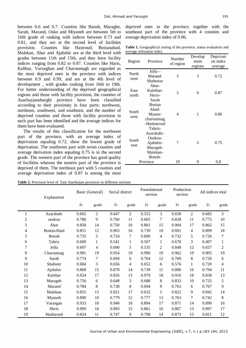
Zali, Ahmadi and Faroughi
Journal of Urban and Environmental Engineering (JUEE), v.7, n.1 p.183-194, 2013
191
between 0.6 and 0.7. Counties like Banab, Maraghe, Sarab, Marand, Osko and Miyaneh are between 5th to 10th grade of ranking with indices between 0.73 and 0.81, and they are at the second level of facilities provision. Counties like Hastroud, Bostanabad, Malekan, Ahar and Ajabshir are at the third level with grades between 11th and 15th, and they have facility indices ranging from 0.82 to 0.87. Counties like Haris, Kalibar, Varzaghan and Charoumagh are regarded as the most deprived ones in the province with indices between 0.9 and 0.99, and are at the 4th level of development , with grades ranking from 16th to 19th. For better understanding of the deprived geographical regions and those with facility provision, the counties of Azarbayjansharghi province have been classified according to their proximity in four parts: northwest, northeast, southwest, and southeast, and the number of deprived counties and those with facility provision in each part has been identified and the average indices for them have been evaluated.
The results of this classification for the northwest part of the province, with an average index of deprivation equaling 0.72, show the lowest grade of deprivation. The southwest part with seven counties and average derivation index equaling 0.75 is in the second grade. The western part of the province has good quality of facilities whereas the eastern part of the province is deprived of them. The northeast part with 5 counties and average deprivation index of 0.87 is among the most
deprived ones in the province, together with the southeast part of the province with 4 counties and average deprivation index of 0.86.
Table 1. Geographical zoning of the province, status evaluation and average utilization index
Region Province Number of region
Development
regions
Deprivation index average
North west
Jolfa –Marand-Shabestar
3 3 0.72
East north
Ahar-Kaleibar-
Heris- Sarab
5 0 0.87
South west
Bostan Abad-
Myane-charouimag-Hashatrood
4 1 0.86
South east
Tabriz-Azarshahr-
Ouskou-Ajabshir-Marageh-Malekan-Bonab-
7 5 0.75
Province 19 9 0.8
Table 2. Provision level of East Azerbaijan provinces in different sections
All indices total Production
section Foundational
section Social district Basic (General)
gradeFi grade Fi gradeFi gradeFi grade Fi
Explanation
3 0.682 2 0.658 3 0.552 2 0.647 2 0.665 Azarshahr 1 10 0.775 11 0.838 7 0.665 11 0.760 9 0.786 ouskou 2 15 0.862 17 0.904 15 0.801 10 0.750 14 0.858 Ahar 3 18 0.899 4 0.681 10 0.739 16 0.903 12 0.851 BostanAbad 4 7 0.726 5 0.732 4 0.600 7 0.724 5 0.735 Bonab 5 1 0.407 3 0.678 1 0.507 1 0.541 1 0.600 Tabriz 6 2 0.657 12 0.848 2 0.535 5 0.690 4 0.697 Jolfa 7
19 0.905 19 0.962 19 0.990 19 0.954 19 0.981 Charoumag 8 6 0.726 8 0.769 12 0.764 6 0.694 7 0.774 Sarab 9 4 0.720 1 0.576 6 0.652 4 0.656 3 0.684 Shabster 10 11 0.794 16 0.896 11 0.739 14 0.878 15 0.868 Ajabshir 11 13 0.838 18 0.910 18 0.979 13 0.826 17 0.924 Kalebar 12 5 0.725 10 0.833 8 0.688 3 0.648 6 0.756 Marageh 13 9 0.767 6 0.763 9 0.694 8 0.738 8 0.784 Marand 14
14 0.842 9 0.822 5 0.632 17 0.921 13 0.855 Malekan 15 8 0.742 7 0.763 13 0.777 12 0.779 10 0.800 Myaneh 16
16 0.890 14 0.871 17 0.894 18 0.940 18 0.933 Varzegan 17 17 0.897 13 0.867 16 0.861 15 0.893 16 0.909 Heris 18 12 0.811 15 0.873 14 0.798 9 0.747 11 0.824 Hashtrood 19
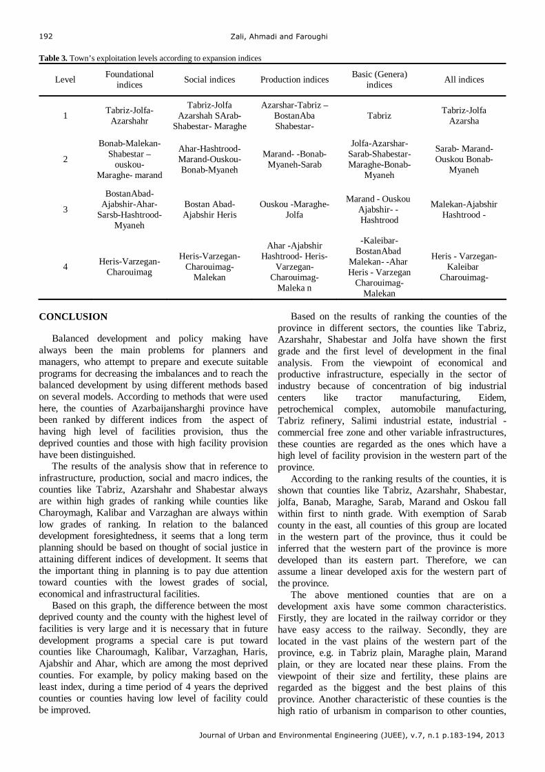
Zali, Ahmadi and Faroughi
Journal of Urban and Environmental Engineering (JUEE), v.7, n.1 p.183-194, 2013
192
Table 3. Town’s exploitation levels according to expansion indices
Level Foundational
indices Social indices Production indices
Basic (Genera) indices
All indices
1 Tabriz-Jolfa-
Azarshahr
Tabriz-Jolfa Azarshah SArab-
Shabestar- Maraghe
Azarshar-Tabriz –BostanAba Shabestar-
Tabriz Tabriz-Jolfa
Azarsha
2
Bonab-Malekan-Shabestar –
ouskou- Maraghe- marand
Ahar-Hashtrood-Marand-Ouskou-Bonab-Myaneh
Marand- -Bonab-Myaneh-Sarab
Jolfa-Azarshar-Sarab-Shabestar-Maraghe-Bonab-
Myaneh
Sarab- Marand- Ouskou Bonab-
Myaneh
3
BostanAbad-Ajabshir-Ahar-
Sarsb-Hashtrood-Myaneh
Bostan Abad-Ajabshir Heris
Ouskou -Maraghe- Jolfa
Marand - Ouskou Ajabshir- - Hashtrood
Malekan-Ajabshir Hashtrood -
4 Heris-Varzegan-
Charouimag
Heris-Varzegan-Charouimag-
Malekan
Ahar -Ajabshir Hashtrood- Heris-
Varzegan-Charouimag-
Maleka n
-Kaleibar- BostanAbad
Malekan- -Ahar Heris - Varzegan
Charouimag- Malekan
Heris - Varzegan-Kaleibar
Charouimag-
CONCLUSION
Balanced development and policy making have
always been the main problems for planners and managers, who attempt to prepare and execute suitable programs for decreasing the imbalances and to reach the balanced development by using different methods based on several models. According to methods that were used here, the counties of Azarbaijansharghi province have been ranked by different indices from the aspect of having high level of facilities provision, thus the deprived counties and those with high facility provision have been distinguished.
The results of the analysis show that in reference to infrastructure, production, social and macro indices, the counties like Tabriz, Azarshahr and Shabestar always are within high grades of ranking while counties like Charoymagh, Kalibar and Varzaghan are always within low grades of ranking. In relation to the balanced development foresightedness, it seems that a long term planning should be based on thought of social justice in attaining different indices of development. It seems that the important thing in planning is to pay due attention toward counties with the lowest grades of social, economical and infrastructural facilities.
Based on this graph, the difference between the most deprived county and the county with the highest level of facilities is very large and it is necessary that in future development programs a special care is put toward counties like Charoumagh, Kalibar, Varzaghan, Haris, Ajabshir and Ahar, which are among the most deprived counties. For example, by policy making based on the least index, during a time period of 4 years the deprived counties or counties having low level of facility could be improved.
Based on the results of ranking the counties of the province in different sectors, the counties like Tabriz, Azarshahr, Shabestar and Jolfa have shown the first grade and the first level of development in the final analysis. From the viewpoint of economical and productive infrastructure, especially in the sector of industry because of concentration of big industrial centers like tractor manufacturing, Eidem, petrochemical complex, automobile manufacturing, Tabriz refinery, Salimi industrial estate, industrial - commercial free zone and other variable infrastructures, these counties are regarded as the ones which have a high level of facility provision in the western part of the province.
According to the ranking results of the counties, it is shown that counties like Tabriz, Azarshahr, Shabestar, jolfa, Banab, Maraghe, Sarab, Marand and Oskou fall within first to ninth grade. With exemption of Sarab county in the east, all counties of this group are located in the western part of the province, thus it could be inferred that the western part of the province is more developed than its eastern part. Therefore, we can assume a linear developed axis for the western part of the province.
The above mentioned counties that are on a development axis have some common characteristics. Firstly, they are located in the railway corridor or they have easy access to the railway. Secondly, they are located in the vast plains of the western part of the province, e.g. in Tabriz plain, Maraghe plain, Marand plain, or they are located near these plains. From the viewpoint of their size and fertility, these plains are regarded as the biggest and the best plains of this province. Another characteristic of these counties is the high ratio of urbanism in comparison to other counties,
Zali, Ahmadi and Faroughi
Journal of Urban and Environmental Engineering (JUEE), v.7, n.1 p.183-194, 2013
193
so that counties of the first rank, which are located in the western part of the province are 75% urbanized in average. Even if we exclude the Tabriz county from this group, the average level of urbanization is again higher than 55%. On the other hand, other counties that are manly located in the eastern part of the province have in average 30% of urbanized population. By this analysis there is a direct correlation between the level of urbanization and the degree of development. The development axis that is located in the western part of the province shows a concentration of facilities, services and urban population, while the axis of underdevelopment in the eastern part of the province includes rural societies with low infrastructure facilities and weak communication networks.
According to the linear development axis in the western part of the province, and according to formation of two completely different parts which are either deprived or with high facility provision, the priority of investment is in the eastern parts of the province. This point must be stressed that if there is a will to reach development in its real concept, when special attention should be made towards adequate distribution of facilities and population in geographical space of a region. Meanwhile, only those kinds of programs whose initial point would be how to deal with growth and development in deprived regions, could reach the desired goals.
Production as an index that is directly correlated with the amount of investments of government or private sector, and with the level of infrastructure provision indices, in counties like Charoumagh, Kalibar, Ahar, Ajabshir, Hashtroud, Varzeghan and Haris is low due to environmental and natural characteristics of these counties and due to centralized management decisions on services distribution, economical and social activities. Although there are some natural and environmental impediments in the above mentioned counties, there are also some unique activities here, hence their improvement could be based on economical and social dynamism and their deprivation grade could decrease especially because of the existence of valuable mines.
From the viewpoint of macro indices there is a similar status. In comparison to other counties of the province, the counties like Charoumagh, Bostanabad, Haris, Varzeghan, Ahar, Malekan and Kalibar got worse conditions, and there is an urgent need to pay attention to these counties. The results show that counties Charoumagh, Varzeghan, Kalibar and Haris are among the most deprived ones according to the infrastructure, social, production and macro indices. Also, the counties like Ahar, Malekan, Bostanabad, Ajabshir and Hashtroud are quite deprived. From the total of 9 deprived counties in the province, 7 are located in its eastern part, whereas only the deprived counties like
Ajabshir and Malekan are located in the western part of the province. REFERENCES
Amini, N. (2006) Ranking health in Iran province. Refah J. 5(1), 27–
48. Antonescu, D. (2012) Identifying regional disparities in Romania: a
convergence process perspective in relation to European Unions territorial structure. Proc. Economics Finan. 3, 1148–1155.
Ardashri, M. (2000) Development, urbanization and urban development policies. City J. 8(1), 13–21
Baldwin, R., Forslid, R., Martin, P., Ottaviano, G. & Robert-Nicoud, F. (2003) Economic Geography and Public Policy, Princeton University Press, Princeton.
Baldwin, R.E. (1999) Agglomeration and endogenous capital. Europ. Economic Rev. 43(2), 253– 280.
Barro, R.J. (1991) Economic growth in a cross section of countries. Quart. J. Economics 106(2), 407–443.
Barro, R.J. (2000) Inequality and growth in a panel of countries. J. Economic Growth 5(1), 5–32.
Barro, R.J. & Sala-i-Martin, X. (1995) Economic Growth, McGraw-Hill, New York.
Beheshti, M.-B. (2008) Survey of investment opportunity in Ardabil province, Ardabil MPORG, education and research office.
Beheshti, M-B. (1983) Introduction of taxonomic model, plan and budget organ. East Azarbayajn Province MPORG.
Bidabadi, B. (1983) Taxonomic analysis and apply to development ranking, plan and budget organization, Arak MPORG.
Borzuyan, S. (1995) Identification of development ranking in Mazandaran province. MSc Thesis, Tarbiat Modares University.
Darwent, D. F. (1969) Growth poles and growth centers in regional planning. Environ. Plann. A 1(1), 5–32.
Feenstra, R.C. (2004) Advanced International Trade: Theory and Evidence, Princeton University Press, Princeton.
Forbes, K.J. (2000) A reassessment of the relationship between inequality and growth. Amer. Economic Rev. 90(4), 869–887.
Fujita, M., Krugman, P. & Venables, A.J. (1999) The Spatial Economy: Cities, Regions and International Trade, MIT Press, Cambridge, Massachusetts.
Habibi, A. (1999) Identification of development degree and pattern in regional disparities reduce, plan and budget organization, Ghazvin (MPORG).
Hakimi, A. (1992) Rural development planning, research center of rural development. Tehran.
Hekmati, F.S. (2003) Ranking East Azarbayjan county viewpoint of development, MPORG, Tabriz.
Helpman, E. (1998) The size of regions. In: Pines, D., Sadka, E. & Zilcha, I. (Eds.) Topics in Public Economics. Theoretical and Applied Analysis, Cambridge University Press, 33–54.
Hosaini, S.Y. & Atusa, E. (2000) Province ranking viewpoint of socio-economical indices. Planning Budget J. 49(50), 101–122.
Kalantari, K. (1998) Identification of backward region in Iran, Geogr. Res. Magaz. 48(1), 120–131.
Kanbur, R. (2000) Income distribution and development. In: Atkinson, A.B. and Bourguignon, F. (Eds.) Handbook of Income Distribution, Volume 1, North-Holland, Amsterdam, pp. 791–841.
Krugman, P.R. (1980) Scale economies, product differentiation, and the pattern of trade. Amer. Economic Rev. 70(5), 950–959.
Krugman, P.R. (1991) Increasing returns and economic geography. J. Polit. Economy 99(3), 483–499.
Krugman, P.R. and Livas Elizondo, R. (1996) Trade policy and the third world metropolis. J. Develop. Economics 49(1), 137–150.
Krugman, P.R. & Venables, A.J. (1995) Globalization and the inequality of nations. Quart. J. Economics 110(4), 857–880.
Lucas Jr., R.E. (1988) On the mechanics of economic development. J. Monet. Economics 22(1), 3–42.

Zali, Ahmadi and Faroughi
Journal of Urban and Environmental Engineering (JUEE), v.7, n.1 p.183-194, 2013
194
Martin, P. (1999a) Are European regional policies delivering? Europ. Invest. Bank Pap. 4(2), 10–23.
Martin, P. (1999b) Public policies, regional inequalities and growth. J. Public Economics 73(1), 85–105.
Martin, P. & Ottaviano, G.I. (1999) Growing locations: Industry location in a model of endogenous growth, Europ. Economic Rev. 43(2), 281–302.
Mokhber, A. (1988) Regional development new methods, plan and budget publication, Tehran.
Myrdal, G. (1957) Economic Theory and Underdeveloped Regions, Gerald Duckworth & Co. Ltd., London.
Noorbakhs, F. (1998) The human development index: some technical issues and alternative indexes. J. Int. Develop. 10(5), 589–605.
Noorbakhs, F. (2000) Human development and regional disparities in Iran, A policy model. University of Glasgow, Department of Economics.
Paas, T. & Tafenau, E. (2009) Regional Disparities and Sustainable Economic Growth. In: Insights into the Sustainable Growth of Business: Modern Management Research Conference; Vilnius, Lithuania; November 19-21, 2009. (CD-ROM).
process perspective in relation to European unions teritorial structures, conference of Emerging Markets Queries in Finance and Business. Proc. Economics Finan. 3, 1148–1155.
Romer P.M. (1986) Increasing returns and long run growth. J. Political Econ. 94(5), 1002–1037.
Romer, P.M. (1990) Endogenous technological change. J. Political Econ. 98(5), S71–S102.
Safaee, M. (1999) Spatial planning in rural centers. MSc Thesis, Shiran, Iran.
Saraffi, M. (1998) Regional development planning, plan and budget organization, Tehran.
Sharbatoghlie, A. (1991) Urbanization and regional disparities in post revolutionary Iran, westriew press. Oxford.
Solow R. M. (2001) Applying Growth Theory across Countries. World Bank Economic Rev. 15(2), 283–288.
Solow R.M. (1956) A contribution to the theory of economic growth. Quart. J. Economics 70(1), 65–94.
Tagvaei, M., Varesi, H.R, Shaykh Baygloo, R. (2012) Analysis of Regional Development Inequalities in Iran. Human Geogr. Res. Quart. 78(1), 23–24.
Vahabi, B. (2000) Distribution of national goals in regional base. Plan. Budget J. 49(1), 27–64.
Zali, N. (2000) Ranking regional development (East Azarbayjan province). MSc Thesis, University of Shiraz, Iran.