A relaxed constant positive linear dependence constraint

qualification and applications ∗

Roberto Andreani† Gabriel Haeser‡ Marıa Laura Schuverdt§

Paulo J. S. Silva¶

October 27, 2010

Abstract

In this work we introduce a relaxed version of the constant positive linear dependence con-straint qualification (CPLD) that we call RCPLD. This development is inspired by a recentgeneralization of the constant rank constraint qualification from Minchenko and Stakhovskithat was called RCR. We show that RCPLD is enough to ensure the convergence of an aug-mented Lagrangian algorithm and asserts the validity of an error bound. We also provideproofs and counter-examples that show the relations of RCR and RCPLD with other knownconstraint qualifications, in particular, RCPLD is strictly weaker than CPLD and RCR, whilestill stronger than Abadie’s constraint qualification. We also verify that RCR is a strongsecond order constraint qualification.Key words: Nonlinear Programming, Constraint Qualifications, Practical Algorithms.AMS Subject Classification: 90C30, 49K99, 65K05.

1 Introduction

In this paper, we consider the nonlinear programming problem

Minimize f(x), subject to x ∈ Ω, (1)

where Ω = {x ∈ ℝn ∣ ℎ(x) = 0, g(x) ≤ 0}, f : ℝn → ℝ, ℎ : ℝn → ℝm and g : ℝn → ℝp arecontinuously differentiable functions. For each feasible point x ∈ Ω, we define the set of activeinequality constraints A(x) = {j ∣ gj(x) = 0, j = 1, . . . , p}.

We say that the constraints defining the feasible set Ω satisfy a constraint qualification if,independently of the objective function f , for every local solution x of (1), there exist Lagrange

∗This work was supported by PRONEX-Optimization (PRONEX-CNPq/FAPERJ E-26/171.510/2006-APQ1),Fapesp (Grants 2006/53768-0 and 2009/09414-7) and CNPq (Grants 300900/2009-0, 303030/2007-0 and474138/2008-9).†Department of Applied Mathematics, Institute of Mathematics, Statistics and Scientific Computing, University

of Campinas, Campinas SP, Brazil. E-mail: andreani@ime.unicamp.br‡Institute of Mathematics and Statistics, University of Sao Paulo, Sao Paulo SP, Brazil. On leave to In-

stitute of Science and Technology, Federal University of Sao Paulo, Sao Jose dos Campos SP, Brazil. E-mail:gabriel.haeser@unifesp.br§CONICET, Department of Mathematics, FCE, University of La Plata, CP 172, 1900 La Plata Bs. As., Ar-

gentina. E-mail: schuverd@mate.unlp.edu.ar¶Institute of Mathematics and Statistics, University of Sao Paulo, Sao Paulo SP, Brazil. E-mail: pjs-

silva@ime.usp.br

1

multipliers � ∈ ℝm and �i ≥ 0 for every i ∈ A(x) such that the KKT condition holds:

∇f(x) +

m∑i=1

�i∇ℎi(x) +∑i∈A(x)

�i∇gi(x) = 0.

Constraint qualifications are properties of the analytical description of the feasible set that en-sure that the reconstruction of its geometrical structure from first order information is possible. Thepresence of a constraint qualification is then fundamental to derive (analytical) characterizationsof the solutions to optimization and variational problems, as well as other theoretical propertiesrelated to duality and sensitivity. It is also essential in the development of computational methodsand to study their convergence.

In this sense, we emphasize two desirable aspects of constraint qualifications. First, they shouldbe associated to practical algorithms, unveiling weak conditions that ensure convergence. Second,they should assert that sensitivity information that may be used for practical purposes can bereadily computed. One good example of such property is the presence of an error bound thatcan be used to analyze the convergence of computational methods. The error bound property,also known as R-regularity, was introduced by Ioffe [14] and explored by Robinson to study theLipschitz properties of multifunctions [22] .

The most common constraint qualification is the linear independence constraint qualification(LICQ), which requires that the gradient vectors

({∇ℎi(x)}mi=1, {∇gi(x)}i∈A(x)

)are linearly in-

dependent. A weaker condition is the Mangasarian-Fromovitz constraint qualification (MFCQ,[17, 23]), which requires only positive-linear independence of the gradient vectors1.

Next, we define the constant rank constraint qualification of Janin (CRCQ, [15]), which is alsoweaker than LICQ.

Definition 1 (CRCQ) We say that the constant rank constraint qualification (CRCQ) holds ata feasible point x ∈ Ω if there exists a neighborhood N(x) of x such that for every I ⊂ {1, . . . ,m}and every J ⊂ A(x), the family of gradients {∇ℎi(y)}i∈I ∪ {∇gi(y)}i∈J has the same rank forevery y ∈ N(x).

In [18], Minchenko and Stakhovski provide a relaxed form of the constant rank constraintqualification, which they called relaxed constant rank (RCR). Instead of requiring that the rankof every subset of equality and active inequality gradients to remain constant in a neighborhoodof a feasible point, they only require constant rank of subsets consisting of all equality gradientsand any subset of active inequality gradients. The authors proved that this is still a constraintqualification, and they used it to prove an error bound property.

It is well known that CRCQ can be equivalently stated as a constant linear dependence condi-tion, that is: for every I ⊂ {1, . . . ,m} and every J ⊂ A(x), whenever {∇ℎi(x)}i∈I ∪{∇gi(x)}i∈J islinearly dependent, we must have {∇ℎi(y)}i∈I∪{∇gi(y)}i∈J linearly dependent for every y ∈ N(x),for some neighborhood N(x) of x.

This motivates the definition of the constant positive linear dependence constraint qualification(CPLD, [21, 6]), which is weaker than MFCQ and CRCQ.

Definition 2 (CPLD) We say that the constant positive linear dependence condition (CPLD)holds at a feasible point x ∈ Ω if there exists a neighborhood N(x) of x such that for everyI ⊂ {1, . . . ,m} and every J ⊂ A(x), whenever ({∇ℎi(x)}i∈I , {∇gi(x)}i∈J) is positive-linearlydependent, then {∇ℎi(y)}i∈I ∪ {∇gi(y)}i∈J is linearly dependent for every y ∈ N(x).

1The pair of families({vi}mi=1, {vi}

pi=m+1

)is said to be positive-linearly dependent if {vi}pi=1 is linearly depen-

dent with non-negative scalars associated to the second family of vectors. Otherwise we say that the pair of familiesis positive-linearly independent.

2

The CPLD is an interesting constraint qualification. Up to now, it is the weakest constraintqualification associated to the convergence of a practical augmented Lagrangian algorithm [2, 3],and it is also sufficient to ensure R-regularity [18]. In this last paper, the authors left open thequestion if the CPLD can be weakened in the same way RCR weakens CRCQ. In this work we willanswer this question affirmatively introducing a relaxed version of the CPLD, that we call RCPLD.We will also extend the result on the convergence of the augmented Lagrangian algorithm and theerror bound property to RCPLD. We provide proofs and counter-examples that give a completepicture of the relationship of RCR and RCPLD with other well known constraint qualifications.

We will use the following notation:

∙ ∥ ⋅ ∥ = ∥ ⋅ ∥2,

∙ ∣J ∣ denotes the number of elements of the finite set J ,

∙ span{vi}mi=1 denotes the subspace generated by the vectors v1, . . . , vm.

2 Relaxed constant rank constraint qualification

We study the relaxed constant rank constraint qualification of Minchenko and Stakhovski (RCR,[18]).

Definition 3 (RCR) We say that the relaxed constant rank condition (RCR) holds at a feasiblepoint x ∈ Ω if there exists a neighborhood N(x) of x such that for every J ⊂ A(x), the family ofgradients {∇ℎi(y)}mi=1 ∪ {∇gi(y)}i∈J has the same rank for every y ∈ N(x).

Compared to original CRCQ this relaxation treats the set of equality constraints as a whole,without the need to impose restrictions on all their subsets. In [18], the authors proved that RCRis still a constraint qualification, by showing that it implies Abadie’s constraint qualification [1].They also showed that RCR is strictly weaker than CRCQ. In the case of only equality constraints,this condition was independently formulated in [4]. The RCR condition has also been studied inthe context of parametric problems in [16].

Since CRCQ is equivalent to the fact that for every subset of equality and active inequalitygradients, linearly dependent vectors remain linearly dependent on some neighborhood, one couldconjecture that a similar equivalence holds true for RCR, considering only subsets that containevery equality gradient. But this is not the case. Consider the equality constraints ℎ1(x1, x2) =x1, ℎ2(x1, x2) = x1 and the inequality constraint g1(x1, x2) = x2

2 at the feasible point x = (0, 0).RCR does not hold since {∇ℎ1(y),∇ℎ2(y),∇g1(y)} has rank one at y = x and rank two for yarbitrarily close to x, but subsets that contain both equality gradients are linearly dependent onevery neighborhood of x.

We will provide a reformulation of RCR in terms of constant linear dependence. We mustkeep the condition that the rank of the equality constraints gradients {∇ℎi(y)}mi=1 is constantfor every y in some neighborhood N(x) of x. The key point is that in that situation, we maychoose a subset I ⊂ {1, . . . ,m} such that {∇ℎi(x)}i∈I is a basis for span{∇ℎi(x)}mi=1, thus, sincelinearly independent vectors remain linearly independent in a neighborhood, and the rank is thesame, we have that {∇ℎi(y)}i∈I is a basis for span{∇ℎi(y)}mi=1 for every y in some neighborhoodN(x) of x. The reformulation requires that for every J ⊂ A(x), linear dependence is maintainedin a neighborhood of x whenever {∇ℎi(x)}i∈I ∪ {∇gi(x)}i∈J is linearly dependent. Notice thatwhen {∇ℎi(x)}i∈I ∪ {∇gi(x)}i∈J is linearly dependent, there must exist an index j ∈ J such that∇gj(x) is a linear combination of the remaining gradients, otherwise this would contradict thelinear independence of {∇ℎi(x)}i∈I . In order to prove our reformulation, we need:

3

Lemma 1 If r is the rank of {∇ℎi(x)}mi=1, then there exists a neighborhood N(x) of x such thatthe rank of {∇ℎi(y)}mi=1 is greater than or equal to r, for every y ∈ N(x).

Proof: This is a direct consequence of the fact that linear independence is preserved locally. □

Theorem 1 Let I ⊂ {1, . . . ,m} be such that {∇ℎi(x)}i∈I is a basis for span{∇ℎi(x)}mi=1. Afeasible point x ∈ Ω satisfies RCR if, and only if, there exists a neighborhood N(x) of x such that

∙ {∇ℎi(y)}mi=1 has the same rank for every y ∈ N(x),

∙ For every J ⊂ A(x), if {∇ℎi(x)}i∈I ∪ {∇gi(x)}i∈J is linearly dependent, then{∇ℎi(y)}i∈I ∪ {∇gi(y)}i∈J is linearly dependent for every y ∈ N(x).

Proof: Let x ∈ Ω satisfies RCR. The first claim follows by taking J = ∅ in the definition of RCR.Let J ⊂ A(x) such that {∇ℎi(x)}i∈I ∪ {∇gi(x)}i∈J is linearly dependent. Since the gradientscorresponding to the set I generate the remaining equality constraints gradients in a neighborhood,using RCR we have that the rank of {∇ℎi(y)}i∈I ∪ {∇gi(y)}i∈J is constant for every y in someneighborhood N(x) of x, therefore, this set must be linearly dependent for y ∈ N(x).

To prove the converse let J ⊂ A(x). Choose J ⊂ J such that {∇ℎi(x)}i∈I ∪ {∇gi(x)}i∈Jis a basis for {∇ℎi(x)}i∈I ∪ {∇gi(x)}i∈J . The case J = J is trivial. Now let j ∈ J∖J . As{∇ℎi(x)}i∈I ∪ {∇gi(x)}i∈J∪{j} is linearly dependent, it must remain linearly dependent in N(x).

Hence the rank of {∇ℎi(x)}i∈I ∪ {∇gi(x)}i∈J is not greater than ∣I∣+ ∣J ∣. The result now followsfrom Lemma 1. □

Next we provide counter-examples to show where RCR fits among other well known constraintqualifications. The following counter-example shows that MFCQ does not imply RCR.

Counter-example 1: Consider the inequality constraints g1(x1, x2) = −x2 and g2(x1, x2) =x2

1 − x2 at the feasible point x = (0, 0). Clearly, MFCQ holds. RCR does not hold since{∇g1(y),∇g2(y)} has rank one at y = x and rank two for y arbitrarily close to x.

We say that quasinormality (see [13, 8]) holds at a feasible point x ∈ Ω if whenever∑mi=1 �i∇ℎi(x)+∑

i∈A(x) �i∇gi(x) = 0, there is not any sequence yk → x such that �i ∕= 0 ⇒ �iℎi(yk) > 0 and

�i > 0⇒ gi(yk) > 0 for every k. The following counter-example shows that RCR does not imply

the quasinormality constraint qualification.

Counter-example 2: Consider the equality constraint ℎ1(x1, x2) = −(x1 + 1)2 − x22 + 1 and

the inequality constraints g1(x1, x2) = x21 + (x2 + 1)2 − 1, g2(x1, x2) = −x2, at the feasible point

x = (0, 0). Quasinormality does not hold, since we can write ∇g1(x) + 2∇g2(x) = 0 and by taking

yk =(√

1− (1− 1k )2 + 1

k ,−1k

)we have g1(yk) > 0 and g2(yk) > 0 for every k. RCR holds since

there is a neighborhood N(x) of x such that for every y ∈ N(x), {∇ℎ1(y)} has rank one and{∇ℎ1(y),∇g1(y)}, {∇ℎ1(y),∇g2(y)}, {∇ℎ1(y),∇g1(y),∇g2(y)} has rank two.

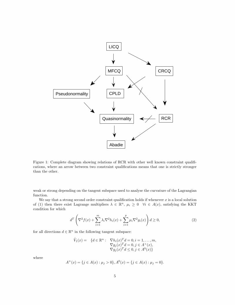
In Figure 1 we show relations of RCR with other well known constraint qualifications, wherepseudonormality is the constraint qualification from [8]. The proof that RCR implies Abadie’sconstraint qualification [1] has been done in [18].

If the problem data is twice continuously differentiable there is the notion of second orderconstraint qualification. As it was mentioned in [4], a second order constraint qualification can be

4

MFCQ

CPLD

RCR

Pseudonormality

Quasinormality

Abadie

CRCQ

LICQ

Figure 1: Complete diagram showing relations of RCR with other well known constraint qualifi-cations, where an arrow between two constraint qualifications means that one is strictly strongerthan the other.

weak or strong depending on the tangent subspace used to analyse the curvature of the Lagrangianfunction.

We say that a strong second order constraint qualification holds if whenever x is a local solutionof (1) then there exist Lagrange multipliers � ∈ ℝn, �i ≥ 0 ∀i ∈ A(x), satisfying the KKTcondition for which

dT

(∇2f(x) +

m∑i=1

�i∇2ℎi(x) +

p∑i=1

�i∇2gi(x)

)d ≥ 0, (2)

for all directions d ∈ ℝn in the following tangent subspace:

V1(x) = {d ∈ ℝn : ∇ℎi(x)T d = 0, i = 1, . . . ,m,∇gj(x)T d = 0, j ∈ A+(x),∇gj(x)T d ≤ 0, j ∈ A0(x)}

whereA+(x) = {j ∈ A(x) : �j > 0}, A0(x) = {j ∈ A(x) : �j = 0}.

5

Analogously, we say that a weak second order constraint qualification holds if there exist atleast one Lagrange multiplier vector such that (2) holds for all directions d ∈ ℝn in the followingsmaller tangent subspace:

V2(x) = {d ∈ ℝn : ∇ℎi(x)T d = 0, i = 1, . . . ,m,∇gj(x)T d = 0, j ∈ A(x)}.

In [4], the authors proved that CRCQ is a strong second order constraint qualification, andthe counter-example defined in [7] shows that MFCQ is not even a weak second order constraintqualification. Thus, considering Figure 1, RCR can still be a second order constraint qualification.Actually, the proof that RCR is a strong second order constraint qualification follows from theRemark 3.2 in [4]. In fact, it was shown in [4] that under RCR, if x is a local solution of (1) then(2) holds for all d ∈ V1(x) and for every Lagrange multiplier vector.

3 Relaxed constant positive linear dependence constraintqualification

In [21], Qi and Wei proposed a relaxation of CRCQ, the constant positive linear dependencecondition (CPLD), taking in consideration the positive sign of the multipliers associated to in-equality constraints in the KKT condition. They used this condition to prove convergence of asequential quadratic programming method.

In [6], it has been proved that CPLD is in fact a constraint qualification, and in [2, 3], theauthors proved convergence of an augmented Lagrangian method under CPLD. We now propose arelaxation of CPLD in a way similar to RCR that we call relaxed CPLD (RCPLD). The definition ismotivated by Theorem 1, considering only positive-linearly dependent gradients, as in the definitionof CPLD.

Definition 4 (RCPLD) Let I ⊂ {1, . . . ,m} be such that {∇ℎi(x)}i∈I is a basis for span{∇ℎi(x)}mi=1.We say that a feasible point x ∈ Ω satisfies the relaxed constant positive linear dependence con-straint qualification (RCPLD) if there exists a neighborhood N(x) of x such that

∙ {∇ℎi(y)}mi=1 has the same rank for every y ∈ N(x),

∙ For every J ⊂ A(x), if ({∇ℎi(x)}i∈I , {∇gi(x)}i∈J) is positive-linearly dependent, then{∇ℎi(y)}i∈I ∪ {∇gi(y)}i∈J is linearly dependent for every y ∈ N(x).

Clearly, Theorem 1 shows that RCR implies RCPLD. It is also clear from the definition thatCPLD implies RCPLD. The constant rank of equality constraints gradients follows from the defi-nition of CPLD with J = ∅ and the equivalence between CRCQ and its definition using constantlinear dependence.

An important tool to deal with positive-linearly dependent vectors (in particular, to deal withCPLD or RCPLD) is Caratheodory’s Lemma [8]. We will state here a similar result that will besuitable to study the RCPLD. This result can be seen as a corollary of Caratheodory’s Lemma,but we include a full proof for completeness.

Lemma 2 If x =

m+p∑i=1

�ivi with vi ∈ ℝn for every i, {vi}mi=1 linearly independent and �i ∕= 0 for

every i = m + 1, . . . ,m + p, then there exist J ⊂ {m + 1, . . . ,m + p} and scalars �i for everyi ∈ {1, . . . ,m} ∪ J such that

∙ x =∑

i∈{1,...,m}∪J

�ivi,

6

∙ �i�i > 0 for every i ∈ J ,

∙ {vi}i∈{1,...,m}∪J is linearly independent.

Proof: We assume that {vi}m+pi=1 is linearly dependent, otherwise the result follows trivially. Then,

there exists � ∈ ℝm+p, such that∑m+pi=m+1 ∣�i∣ > 0 and

∑m+pi=1 �ivi = 0. Thus, we may write

x =∑m+pi=1 (�i − �i)vi, for every ∈ ℝ. Choosing ∕= 0 as the number of smallest modulus such

that �i − �i = 0 for at least one index i ∈ {m + 1, . . . ,m + p}, we are able to write the linearcombination x with at least one vector vi less, for some i ∈ {m + 1, . . . ,m + p}. We may repeatthis procedure until the vectors are linearly independent. □

We point out that we can obtain bounds ∣�i∣ ≤ 2p−1∣�i∣,∀i = m+1, . . . ,m+p in the same wayit is done in [11]. This may be useful, in particular, for applications to interior point methods.

We now prove that RCPLD is a constraint qualification. We will need a definition from [5]:

Definition 5 (AKKT) We say that x ∈ Ω satisfies the Approximate-KKT condition (AKKT) ifthere exist sequences xk → x, {�k} ⊂ ℝm, {�k} ⊂ ℝp, �k ≥ 0 such that

∇f(xk) +

m∑i=1

�ki∇ℎi(xk) +∑i∈A(x)

�ki∇gi(xk)→ 0.

Note that the definition of AKKT also depends on the objective function f , thus, it is a propertyof the optimization problem, rather than only of the constraint set. In Theorem 2.3 of [5] (withI = ∅), the authors proved that every local minimizer fulfills the AKKT condition (a simplerproof, specific for the case I = ∅, can be found in [12]). To prove that RCPLD is a constraintqualification, we need only to show that if RCPLD holds at a feasible point x such that AKKT alsoholds, then x is a KKT point. This property is also important because it ensures the convergenceof an augmented Lagrangian algorithm as we discuss in the next section.

Theorem 2 Let x ∈ Ω be such that RCPLD and AKKT hold, then x is a KKT point.

Proof: From the definition of AKKT, there exist sequences "k → 0, xk → x, �k ∈ ℝm, �kj ≥0,∀j ∈ A(x), such that

∇f(xk) +

m∑i=1

�ki∇ℎi(xk) +∑

j∈A(x)

�kj∇gj(xk) = "k, for every k.

Consider a subset I ⊂ {1, . . . ,m} such that {∇ℎi(x)}i∈I is a basis for span{∇ℎi(x)}mi=1. FromLemma 2, we must have {∇ℎi(xk)}i∈I linearly independent for sufficiently large k, and sincethe rank of equality constraint gradients is constant, we have that {∇ℎi(xk)}i∈I is a basis forspan{∇ℎi(xk)}mi=1 for sufficiently large k. Thus, there exist a sequence {�k} ⊂ ℝ∣I∣ such that∑mi=1 �

ki∇ℎi(xk) =

∑i∈I �

ki∇ℎi(xk), and we may write

∇f(xk) +∑i∈I

�ki∇ℎi(xk) +∑

j∈A(x)

�kj∇gj(xk) = "k.

We apply Lemma 2 to obtain subsets Jk ⊂ A(x) and multipliers �k ∈ ℝ∣I∣ and �kj ≥ 0,∀j ∈ Jksuch that

∇f(xk) +∑i∈I

�ki∇ℎi(xk) +∑j∈Jk

�kj∇gj(xk) = "k,

7

and {∇ℎi(xk)}i∈I ∪ {∇gi(xk)}i∈Jk is linearly independent. We will consider a subsequence suchthat Jk is the same set J for every k (this can be done since there are finitely many possible setsJk). Define Mk = max{∣�ki ∣,∀i ∈ I, �kj ,∀j ∈ J}. If there is a subsequence such that Mk → +∞,

we may take a subsequence such that(�k,�k)Mk

→ (�, �) ∕= 0, � ≥ 0. Dividing by Mk and takinglimits we have ∑

i∈I�i∇ℎi(x) +

∑j∈J

�j∇gj(x) = 0,

which contradicts RCPLD. Hence, we have that {Mk} is a bounded sequence. Taking limits for asuitable subsequence such that �k → � and �k → � ≥ 0 we have

∇f(x) +

m∑i=1

�i∇ℎi(x) +∑j∈J

�j∇gj(x) = 0,

which proves that x is a KKT point. □

Corollary 1 RCPLD is a constraint qualification.

Given a new constraint qualification, it is important to know its relation with other well knownconstraint qualifications. In particular, we would like to know if RCPLD can still guarantee thatthe tangent cone is polyhedral. In the following theorem we prove that this is the case by showingthat RCPLD implies Abadie’s constraint qualification.

Let us consider the feasible set Ω and x ∈ Ω. We define the (upper) tangent cone of Ω at x as(see for example [8, 10, 13, 25]):

TΩ(x) = {0}∪{d ∈ ℝn : there exists a sequence {xk} ⊂ Ω, xk ∕= x, xk → x and

xk − x∥xk − x∥

→ d

∥d∥

}.

(3)We define also the linearized tangent cone at x as:

VΩ(x) = {d ∈ ℝn : ∇ℎi(x)T d = 0, i = 1, . . . ,m;∇gj(x)T d ≤ 0, j ∈ A(x)}. (4)

We say that Abadie’s constraint qualification [1] holds at a feasible point x ∈ Ω if TΩ(x) =VΩ(x).

Theorem 3 Let x ∈ Ω be such that RCPLD holds, then x satisfies Abadie’s constraint qualifica-tion.

Proof. The inclusion TΩ(x) ⊂ VΩ(x) holds without any constraint qualification for every feasiblepoint x ∈ Ω.

The proof that VΩ(x) ⊂ TΩ(x) relies on a simplification considered in [8, 13]. Let us define theset of indexes

J = {i ∈ A(x) : ∇gi(x)T d = 0, ∀d ∈ VΩ(x)}.

DefineX = {x ∈ ℝn : ℎi(x) = 0, i = 1, . . . ,m; gj(x) ≤ 0, j ∈ J}.

In the degenerate case, where there are no equalities and the set J is empty, we have X = ℝn byconvention. In this case, every point of X verifies RCPLD and Abadie.

By the definition of RCPLD, if a feasible point x ∈ Ω verifies the RCPLD then it verifies theRCPLD as a point in X. Using this simplification, let us prove that x verifies Abadie as a pointin X.

8

We have that TX(x) ⊂ VX(x) always holds. Let us take a direction d ∈ VX(x). Let " > 0,k > 0 and let y(t, k) be the minimizer of the function

H(y, t, k) = ∥y − x− td∥2 + tk

⎛⎝ m∑i=1

ℎi(y)2 +∑i∈J

max{0, gi(y)}2⎞⎠

subject to ∥y − x∥ ≤ ".We have that, for t ≥ 0,

∥y(t, k)− x− td∥2 ≤ H(y(t, k), t, k) ≤ H(x, t, k) = t2∥d∥2, (5)

and analogously

0 ≤ k

⎛⎝ m∑i=1

ℎi(y(t, k))2 +∑i∈J

max{0, gi(y(t, k))}2⎞⎠ ≤ t∥d∥2. (6)

By (5) we have∥y(t, k)− x∥ ≤ 2t∥d∥. (7)

Thus, for each t > 0, we have that the sequence {y(t, k)}k is a bounded sequence and thereexists y(t), t > 0 such that, taking a subsequence if necessary, we have

y(t, k)→ y(t). (8)

Then, taking limits in (6) and by continuity:

0 ≤

⎛⎝ m∑i=1

ℎi(y(t))2 +∑i∈J

max{0, gi(y(t))}2⎞⎠ ≤ lim

k→∞

t

k∥d∥2 = 0.

This implies that y(t) ∈ X for all t > 0.From (7) we have that y(t) → x as t → 0. Moreover, we can select a sequence of positive

numbers tr with tr → 0 such that the limit

d0 = limr→∞

y(tr)− xtr

exists. Since y(t) ∈ X for all t > 0 we obtain that d0 ∈ TX(x) ⊂ VX(x).Let us consider r0 large enough such that, by (7), ∥y(tr, k) − x∥ < ", ∀r ≥ r0,∀k. By the

definition of y(t, k) we have that, for r ≥ r0, ∇yH(y(tr, k), tr, k) = 0, then

y(tr, k)− x− trdtr

+ k

⎛⎝ m∑i=1

ℎi(y(tr, k))∇ℎi(y(tr, k)) +∑i∈J

max{0, gi(y(tr, k))}∇gi(y(tr, k))

⎞⎠ = 0.

By the definition of RCPLD, we may take a subset I ⊂ {1, . . . ,m} such that {∇ℎi(y(tr, k))}i∈I is abasis for span{∇ℎi(y(tr, k))}mi=1 for sufficiently large k. Thus, there exist a sequence {�k(r)} ⊂ ℝmsuch that

∑mi=1 kℎi(y(tr, k))∇ℎi(y(tr, k)) =

∑i∈I �

ki (r)∇ℎi(y(tr, k)). By applying Lemma 2, we

have that there are subsets Jk(r) ⊂ J and multipliers �ki (r),∀i ∈ I and �ki (r) ≥ 0,∀i ∈ Jk(r) suchthat

y(tr, k)− x− trdtr

+∑i∈I

�ki (r)∇ℎi(y(tr, k)) +∑

i∈Jk(r)

�ki (r)∇gi(y(tr, k)) = 0 (9)

9

and{∇ℎi(y(tr, k))}i∈I ∪ {∇gi(y(tr, k))}i∈Jk(r) is linearly independent. (10)

We will consider a subsequence such that Jk(r) is the same set J(r) (this can be done since thereare finitely many possible sets Jk(r)).

Denote,

Mk(r) =

√1 +

∑i∈I

(�ki (r))2 +∑i∈J(r)

(�ki (r))2.

Then, dividing (9) by Mk(r) and taking limit when k → ∞ for k in an appropriate subsequencewe have that there are scalars �0(r), �i(r), i ∈ I, �j(r), j ∈ J(r), �j(r) ≥ 0 not all equal to zerosuch that

�0(r)

(y(tr)− x

tr− d)

+∑i∈I

�i(r)∇ℎi(y(tr)) +∑i∈J(r)

�i(r)∇gi(y(tr)) = 0, for tr > 0. (11)

Let us consider a subsequence such that J(r) is the same set J . Using that ∥(�0(r), �i(r), �i(r))∥ =1 and taking limit when r →∞ for r in an appropriate subsequence in (11) we have that there arescalars �0, �i, i ∈ I, �j , j ∈ J, �j ≥ 0 not all equal to zero such that

�0(d0 − d) +∑i∈I

�i∇ℎi(x) +∑i∈J

�i∇gi(x) = 0.

If �0 = 0, then we have that ({∇ℎi(x)}i∈I , {∇gi(x)}i∈J) is positive-linearly dependent, hence,

since (10) holds, this contradicts RCPLD. Consequently, it must be �0 > 0. Given d ∈ VX(x),

let us prove that ∇gj(x)T d = 0 for every j ∈ J . From the definition of VX(x) we have that

∇gj(x)T d ≤ 0 for every j ∈ J , and from the definition of J , for every i ∈ A(x)∖J there exists

di ∈ VΩ(x) such that ∇gi(x)T di < 0. Defining d =∑

i∈A(x)∖J

di, we have that

∇gi(x)T d < 0 for every i ∈ A(x)∖J ,

and∇gj(x)T d = 0 for every j ∈ J .

Thus, for sufficiently large � > 0 we have

∇gi(x)T (d+ �d) = ∇gi(x)T d+ �∇gi(x)T d < 0 for every i ∈ A(x)∖J ,

and∇gj(x)T (d+ �d) = ∇gj(x)T d ≤ 0 for every j ∈ J .

Hence d + �d ∈ VΩ(x), which implies that for all j ∈ J ,∇gj(x)T (d + �d) = ∇gj(x)T d = 0 as wewanted to prove. Thus, multiplying (11) by d, d0 ∈ VX(x), we obtain that

dT0 (d− d0) = 0 = dT (d− d0),

which implies that d = d0 ∈ TX(x).

We have proved that a feasible point x that verifies RCPLD as a point in X verifies Abadie’sas a point in X.

Now we have to prove that this implies that x verifies Abadie as a point in Ω. Let us definethe set VΩ(x) = {d ∈ ℝn : ∇ℎi(x)T d = 0, i = 1, . . . ,m;∇gj(x)T d = 0, j ∈ J ;∇gj(x)T d < 0, j ∈A(x)∖J}.

10

Since x verifies that TX(x) = VX(x) and VΩ(x) ⊂ VX(x) it is possible to prove that VΩ(x) ⊂TΩ(x). In general, TΩ(x) is a closed cone, thus, VΩ(x) = cl(VΩ(x)) ⊂ TΩ(x), where cl(⋅) denotesthe closure operator. Thus, we have that x verifies Abadie as a point in Ω as we wanted to prove. □

We will now provide some counter-examples to completely state the relation of RCPLD withrespect to other known constraint qualifications. We observe that since MFCQ implies RCPLD,Counter-example 1 shows that RCR is strictly stronger than RCPLD.

We say that pseudonormality (see [8]) holds at a feasible point x ∈ Ω if whenever∑mi=1 �i∇ℎi(x)+∑

i∈A(x) �i∇gi(x) = 0, there is not any sequence yk → x such that∑mi=1 �iℎi(y

k)+∑i∈A(x) �igi(y

k) >0 for every k.

The following counter-example shows that pseudonormality does not imply RCPLD.

Counter-example 3: Consider the inequality constraints g1(x1, x2) = −x1, g2(x1, x2) = x1 −x2

1x22, at the feasible point x = (0, 0). RCPLD does not hold since (∅, {∇g1(y),∇g2(y)}) is positive-

linearly dependent at y = x but linearly independent for y arbitrarily close to x. Pseudonormalityholds, since we can write �∇g1(x) + �∇g2(x) = 0 for every � > 0, but �g1(y1, y2) + �g2(y1, y2) =−�y2

1y22 ≤ 0 for every y.

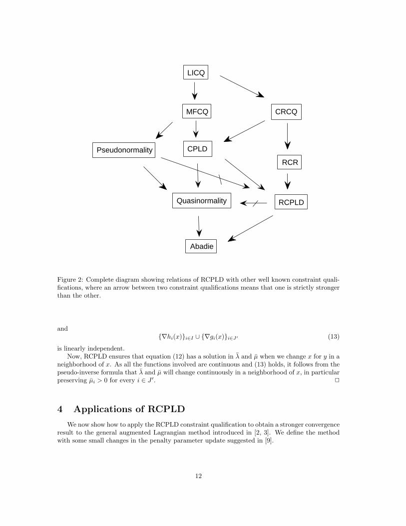
Since RCR does not imply quasinormality and RCR implies RCPLD, we have that RCPLDdoes not imply quasinormality. In Figure 2 we show a complete diagram picturing the relations ofRCPLD with other constraint qualifications.

Observe that, since MFCQ is not a second order constraint qualification and MFCQ impliesRCPLD, this shows that RCPLD cannot be a second order constraint qualification.

It can be proved (see [24]) that the CPLD condition can be equivalently stated at a feasible pointx ∈ Ω as: for every subset I ⊂ {1, . . . ,m} and J ⊂ A(x), whenever ({∇ℎi(x)}i∈I , {∇gi(x)}i∈J) ispositive-linearly dependent, we have that ({∇ℎi(y)}i∈I , {∇gi(y)}i∈J) is positive-linearly dependentfor every y in some neighborhood of x. That is, requiring that the gradients are positive-linearlydependent in a neighborhood instead of the apparently weaker requirement of linear dependence,is in fact the same thing. This is an aesthetically pleasant result, that also guarantees that CPLDis stable in the sense that if a feasible point x ∈ Ω satisfies CPLD, then every feasible point insome neighborhood of x will also satisfy CPLD. We will prove an analogous equivalent definitionfor RCPLD that also guarantees stability of RCPLD.

Theorem 4 Let I ⊂ {1, . . . ,m} be such that {∇ℎi(x)}i∈I is a basis for span{∇ℎi(x)}mi=1. Afeasible point x ∈ Ω satisfies RCPLD if, and only if, there exists a neighborhood N(x) of x suchthat

∙ {∇ℎi(y)}mi=1 has the same rank for every y ∈ N(x),

∙ For every J ⊂ A(x), if ({∇ℎi(x)}i∈I , {∇gi(x)}i∈J) is positive-linearly dependent, then({∇ℎi(y)}i∈I , {∇gi(y)}i∈J) is positive-linearly dependent for every y ∈ N(x).

Proof: Let us take x ∈ Ω that satisfies RCPLD and J ⊂ A(x) such that ({∇ℎi(x)}i∈I , {∇gi(x)}i∈J)is positive-linearly dependent. Thus, there exist �i ∈ ℝ,∀i ∈ I, �i ≥ 0,∀i ∈ J,

∑i∈J �i > 0 such

that∑i∈I �i∇ℎi(x) +

∑i∈J �i∇gi(x) = 0. We can assume that �i > 0 for every i ∈ J . Since

J ∕= ∅, taking j ∈ J we may write �j∇gj(x) =∑i∈I −�i∇ℎi(x)+

∑i∈J∖{j}−�i∇gi(x). By Lemma

2, there exist J ′ ⊂ J∖{j} and �i ∈ ℝ,∀i ∈ I, �i > 0,∀i ∈ J ′ such that

�j∇gj(x) =∑i∈I−�i∇ℎi(x) +

∑i∈J′−�i∇gi(x) (12)

11

CPLDPseudonormality

Quasinormality

Abadie

RCR

RCPLD

MFCQ

LICQ

CRCQ

Figure 2: Complete diagram showing relations of RCPLD with other well known constraint quali-fications, where an arrow between two constraint qualifications means that one is strictly strongerthan the other.

and{∇ℎi(x)}i∈I ∪ {∇gi(x)}i∈J′ (13)

is linearly independent.Now, RCPLD ensures that equation (12) has a solution in � and � when we change x for y in a

neighborhood of x. As all the functions involved are continuous and (13) holds, it follows from thepseudo-inverse formula that � and � will change continuously in a neighborhood of x, in particularpreserving �i > 0 for every i ∈ J ′. □

4 Applications of RCPLD

We now show how to apply the RCPLD constraint qualification to obtain a stronger convergenceresult to the general augmented Lagrangian method introduced in [2, 3]. We define the methodwith some small changes in the penalty parameter update suggested in [9].

12

We consider the problem

Minimize f(x), subject to ℎ(x) = 0, g(x) ≤ 0, ℎ(x) = 0, g(x) ≤ 0, (14)

where f : ℝn → ℝ, ℎ : ℝn → ℝm, g : ℝn → ℝp, ℎ : ℝn → ℝm and g : ℝn → ℝp are continuouslydifferentiable functions. When the constraints ℎ(x) = 0 and g(x) ≤ 0 define a box in ℝn, this

is the algorithm implemented in ALGENCAN2. Given � > 0, � ∈ ℝm, � ∈ ℝp, � ≥ 0, x ∈ ℝn wedefine the augmented Lagrangian function

ℒ�(x, �, �) = f(x) +�

2

(∥∥∥∥ℎ(x) +�

�

∥∥∥∥2

+

∥∥∥∥max

{0, g(x) +

�

�

}∥∥∥∥2). (15)

Algorithm Let "k ≥ 0, "k → 0, �k ∈ [�min, �max]m, �k ∈ [0, �max]

pfor all k, �1 > 0, � ∈

(0, 1), � > 1.For all k, compute xk ∈ ℝn such that there exist vk ∈ ℝm, wk ∈ ℝp, wk ≥ 0 satisfying:∥∥∥∥∥∇xℒ�k(xk, �k, �k) +

m∑i=1

vki∇ℎi(xk) +

p∑i=1

wki∇gi(xk)

∥∥∥∥∥ ≤ "k, (16)

∥ℎ(xk)∥ ≤ "k, ∥max{0, g(xk)}∥ ≤ "k, (17)

andwki = 0 whenever g

i(xk) < −"k. (18)

We define, for all i = 1, . . . , p,

V ki = max

{gi(x

k),−�ki�k

}. (19)

If k = 1 ormax{∥ℎ(xk)∥, ∥V k∥} ≤ � max{∥ℎ(xk−1)∥, ∥V k−1∥} (20)

we define �k+1 ≥ �k. Else, we define �k+1 ≥ ��k.

Remark: We can define the multiplier sequences {�k} and {�k} using for example the firstorder update formula �k+1

i = P[�min,�max]m(�ki +�kℎi(xk)), i = 1, . . . ,m and �k+1

i = P[0,�max]p(�ki +

�kgi(xk)), i = 1, . . . , p, where PX(⋅) denotes the euclidean projection in X.

Theorem 5 If x∗ is a limit point of a sequence generated by the Algorithm, then x∗ is an AKKTpoint of the problem

Minimize ∥ℎ(x)∥2 + ∥max{0, g(x)}∥2, subject to ℎ(x) = 0, g(x) ≤ 0. (21)

Proof: Consider a subsequence such that xk → x∗. Since "k → 0, by (17) we have that ℎ(x∗) = 0and g(x∗) ≤ 0. If {�k} is bounded we have that (20) is satisfied for every sufficiently large k, whichimplies ℎ(x∗) = 0 and g(x∗) ≤ 0. Hence, x∗ is a global minimum for problem (21). Let us assume�k → +∞. By (15) and (16) we have that

∇f(xk) +

m∑i=1

(�ki + �kℎi(xk))∇ℎi(xk) +

p∑i=1

max{0, �ki + �kgi(xk)}∇gi(xk)+

+

m∑i=1

vki∇ℎi(xk) +

p∑i=1

wki∇gi(xk) = �k,

(22)

2freely available at www.ime.usp.br/∼egbirgin/tango

13

where �k → 0. If gi(x∗) < 0, then g

i(xk) < −"k for sufficiently large k, which implies by (18) that

wki = 0 for sufficiently large k. Dividing (22) by �k we may write:

m∑i=1

ℎi(xk)∇ℎi(xk) +

p∑i=1

max{0, gi(xk)}∇gi(xk) +

m∑i=1

vki�k∇ℎi(xk) +

∑gi(x∗)=0

wki�k∇g

i(xk)

=�k

�k− ∇f(xk)

�k−

m∑i=1

�ki�k∇ℎi(xk) +

p∑i=1

(max{0, gi(xk)} −max

{0,�ki�k

+ gi(xk)

})∇gi(xk).

(23)Since {�k} and {�k} are bounded sequences, the right hand side of (23) goes to zero, thus x∗

satisfies the AKKT condition for problem (21). □

Theorem 6 If x∗ is a limit point of a sequence generated by the Algorithm such that x∗ is feasiblefor (14), then x∗ is an AKKT point of problem (14).

Proof: By (15) and (16) we have that (22) holds, where �k → 0. As in the proof of Theorem 5we have that if g

i(x∗) < 0 then wki = 0 for sufficiently large k. Define �ki = �ki + �kℎi(x

k) and

�ki = max{0, �ki + �kgi(xk)} ≥ 0. Now let us assume gi(x

∗) < 0. If {�k} is unbounded, then�ki + �kgi(x

k) < 0, hence �ki = 0 for sufficiently large k. If {�k} is bounded we have that (20)is satisfied for every sufficiently large k, hence V ki → 0, which implies by (19) that �ki → 0, thus�ki = 0 for sufficiently large k. Then, we may write (22) as:

∇f(xk) +

m∑i=1

�ki∇ℎi(xk) +∑

gi(x∗)=0

�ki∇gi(xk)+

+

m∑i=1

vki∇ℎi(xk) +∑

gi(x∗)=0

wki∇gi(xk) = �k,

(24)

hence x∗ satisfies the AKKT condition for problem (14). □

Applying Theorem 2 we may sate the following:

Corollary 2 If x∗ is a limit point of a sequence generated by the Algorithm, then one of thefollowing holds:

∙ x∗ is a feasible point of (14).

∙ x∗ is a KKT point of the problem

Minimize ∥ℎ(x)∥2 + ∥max{0, g(x)}∥2, subject to ℎ(x) = 0, g(x) ≤ 0. (25)

∙ The constraint set defined by ℎ(x) = 0, g(x) ≤ 0 does not satisfy RCPLD at x∗.

Corollary 3 If x∗ is a limit point of a sequence generated by the Algorithm such that x∗ is feasiblefor (14), then one of the following holds:

∙ x∗ is a KKT point of problem (14).

∙ The constraint set defined by ℎ(x) = 0, g(x) ≤ 0, ℎ(x) = 0, g(x) ≤ 0 does not satisfy RCPLDat x∗.

14

In [3], the authors proved these same convergence theorems but employing a stronger constraintqualification (the CPLD). In particular, our result also shows convergence of this AugmentedLagrangian algorithm under RCR. We point out that we can also use RCPLD to prove convergenceof a version of this augmented Lagrangian algorithm that do not require derivatives [20].

We now show that an error bound property holds under the RCPLD. This has been previouslydone for RCR and CPLD in [18], and alternatively for RCR in [16]. As mentioned in [19, 25],an initial motivation to study error bounds arose from a practical consideration in the computerimplementation of iterative methods for solving optimization and equilibrium programs. An errorbound is an estimate of the distance from a given feasible point in terms of computable quantitiesmeasuring the violation of the constraints. It is associated to a so-called residual function thatplays a central role in the treatment of infeasible mathematical programming problems. We willprove the stronger result that the error bound property holds under RCPLD.

Definition 6 We say that the point x ∈ Ω satisfies the error bound property with respect to theconstraints ℎ(x) = 0 and g(x) ≤ 0 if there exist � > 0 and a neighborhood N(x) of x such that forevery y ∈ N(x)

minz∈Ω∥z − y∥ ≤ �r(y),

where r is a function that measures the infeasibility with respect to Ω that is readily computable.

Theorem 7 If x ∈ Ω satisfies RCPLD and the functions ℎ and g defining Ω admit second deriva-tives in a neighborhood of x, then x satisfies the error bound property with r(y) = max{∥ℎ(y)∥∞, ∥max{0, g(y)}∥∞}.

Proof: If x is in the interior of Ω, then clearly the error bound property holds. We will assumethat x lies in the frontier of Ω. For a fixed y ∈ ℝn, consider the problem

Minimize ∥z − y∥, subject to ℎ(z) = 0, g(z) ≤ 0. (26)

In Theorem 2 of [18], the authors proved that if second derivatives are available, then the errorbound property holds at x ∈ Ω if, and only if, there exists a neighborhood N(x) of x such thatthere exist Lagrange multipliers to problem (26) that lie in a fixed compact set for all y ∈ N(x),y ∕∈ Ω. Let us consider a sequence yk → x, yk ∕∈ Ω and let zk be a solution to (26) for y = yk. Since∥zk − yk∥ ≤ ∥x − yk∥ we have also zk → x. It is a consequence of Theorem 4 that the RCPLDcondition is preserved in a neighborhood, thus zk ∈ Ω also satisfies RCPLD for sufficiently largek. Hence, there exist {�k} ⊂ ℝm and {�k} ⊂ ℝp, �ki ≥ 0 such that

zk − yk

∥zk − yk∥+

m∑i=1

�ki∇ℎi(zk) +∑

i∈A(zk)

�ki∇gi(zk) = 0,

for sufficiently large k, where A(zk) = {i ∈ {1, . . . , p} ∣ gi(zk) = 0}. From the definition of RCPLDwe have that there exist I ⊂ {1, . . . ,m} and �ki for every i ∈ I such that {∇ℎi(zk)}i∈I is linearlyindependent and

∑mi=1 �

ki∇ℎi(zk) =

∑i∈I �

ki∇ℎi(zk) for sufficiently large k, hence, by Lemma 2,

there exist Jk ⊂ A(zk), �ki for every i ∈ I and �ki ≥ 0 for every i ∈ Jk such that:

zk − yk

∥zk − yk∥+∑i∈I

�ki∇ℎi(zk) +∑i∈Jk

�ki∇gi(zk) = 0, (27)

and{∇ℎi(zk)}i∈I ∪ {∇gi(zk)}i∈Jk (28)

is linearly independent. Let us consider a subsequence such that Jk is the same set J for everyk, where J ⊂ A(zk) ⊂ A(x). Define Mk = ∥(�k, �k)∥∞ and let us assume by contradiction that

15

{Mk} is unbounded. Taking a subsequence such that (�k,�k)Mk

→ (�, �) ∕= 0, � ≥ 0, we may divide

(27) by Mk and take limits for this subsequence to obtain:∑i∈I

�i∇ℎi(x) +∑i∈J

�i∇gi(x) = 0.

Since RCPLD holds at x we have that {∇ℎi(zk)}i∈I ∪ {∇gi(zk)}i∈J must be linearly dependentfor sufficiently large k, which contradicts (28). This concludes the proof. □

5 Final Remarks

We introduced a generalization of the RCR constraint qualification called RCPLD. We showedthat this constraint qualification is strictly weaker than RCR and CPLD. The RCPLD shares withCPLD many of its important properties. In particular, it is enough to ensure the convergence ofan Augmented Lagrangian algorithm and the presence of an error bound.

An interesting question that was not touched in this paper is whether it is possible to extendthe RCR in a way that does not involve assumptions on the behavior of the gradients of all subsetsof the active inequality constraints. Such extension would better fit the spirit of RCR when thedescription of the constraint does not have any inequalities. In this case, the assumption of constantrank has to be fulfilled only by the set of all gradients of the constraints.

Another question is whether RCPLD can still be weakened preserving the convergence of aug-mented Lagrangian algorithms. It may be also interesting to investigate its role in the convergenceof other optimization methods, like sequential quadratic programming or inexact-restoration, aswell as in the convergence of the extension of such methods to deal with variational inequalities.Finally, it may be valuable to search for an alternative proof that RCPLD implies the validity of anerror bound that does not depend on the existence of second derivatives as required in Theorem 7.

Acknowledgement

The authors would like to thank Prof. Alexey Izmailov from the Moscow State University forpointing out the work of Minchenko and Stakhovski [18].

References

[1] J. Abadie. On the Kuhn-Tucker theorem. In J. Abadie, editor, Nonlinear Programming, pages21–36. John Wiley, 1967.

[2] R. Andreani, E.G. Birgin, J.M. Martınez, and M.L. Schuverdt. On augmented lagrangianmethods with general lower–level constraints. SIAM Journal on Optimization, 18:1286–1309,2007.

[3] R. Andreani, E.G. Birgin, J.M. Martınez, and M.L. Schuverdt. Augmented lagrangian meth-ods under the constant positive linear dependence constraint qualification. MathematicalProgramming, 112:5–32, 2008.

[4] R. Andreani, C.R. Echague, and M.L. Schuverdt. Constant-rank condition and second-order constraint qualification. Journal of Optimization Theory and Applications, 2010. DOI:10.1007/s10957-010-9671-8.

16

[5] R. Andreani, G. Haeser, and J.M. Martınez. On sequential optimality conditions for smoothconstrained optimization. Optimization, 2010. (to appear). Available at Optimization Onlinehttp://www.optimization-online.org/DB HTML/2009/06/2326.html.

[6] R. Andreani, J.M. Martınez, and M.L. Schuverdt. On the relation between constant positivelinear dependence condition and quasinormality constraint qualification. Journal of Optimiza-tion Theory and Applications, 125:473–485, 2005.

[7] A. V. Arutyunov. Perturbations of extremum problems with constraints and necessary opti-mality conditions. Journal of Soviet Mathematics, 54:1342–1400, 1991.

[8] D.P. Bertsekas. Nonlinear Programming: 2nd Edition. Athena Scientific, 1999.

[9] E. Birgin, L.F. Bueno, N. Krejic, and J.M. Martınez. Low Order-Value approach for solvingVaR-constrained optimization problems. 2010. submitted.

[10] G. Giorgi and A. Guerraggio. On the notion of tangent cone in mathematical programming.Optimization, 25:1:11–23, 1992.

[11] G. Haeser. On the global convergence of interior-point nonlinear programming algorithms.Computational & Applied Mathematics, 2010. (to appear). Available at Optimization Onlinehttp://www.optimization-online.org/DB HTML/2009/06/2332.html.

[12] G. Haeser and M.L. Schuverdt. Approximate KKT condition for continuous vari-ational inequality problems. 2010. submitted. Available at Optimization Onlinehttp://www.optimization-online.org/DB HTML/2009/10/2415.html.

[13] M.R. Hestenes. Optimization theory: the finite dimensional case. John Wiley, 1975.

[14] A.D. Ioffe. Regular points of Lipschitz functions. Transactions of American MathematicalSociety, 251:61–69, 1979.

[15] R. Janin. Directional derivative of the marginal function in nonlinear programming. Mathe-matical Programming Study, 21:110–126, 1984.

[16] S. Lu. Relation between the constant rank and the relaxed constant rank constraint qualifi-cations. 2010. submitted. Available at http://www.unc.edu/∼shulu/.

[17] O.L. Mangasarian and S. Fromovitz. The Fritz John optimality conditions in the presenceof equality and inequality constraints. Journal of Mathematical Analysis and Applications,17:37–47, 1967.

[18] L. Minchenko and S. Stakhovski. On relaxed constant rank regularity condition in mathemat-ical programming. Optimization, 2010. (to appear).

[19] J.-S. Pang. Error bound in mathematical programming. Mathematical Programming, 79:299–332, 1997.

[20] L.G. Pedroso. Programacao nao linear sem derivadas. PhD thesis, IMECC-UNICAMP, Departamento de Matematica Aplicada, Campinas-SP, Brazil, 2009.http://libdigi.unicamp.br/document/?code=000468366.

[21] L. Qi and Z. Wei. On the constant positive linear dependence condition and its applicationto SQP methods. SIAM Journal on Optimization, 10:963–981, 2000.

17

[22] S.M. Robinson. Stability theory for systems of inequalities. part II: Differentiable nonlinearsystems. SIAM Journal on Numerical Analysis, 13(4):497–513, 1976.

[23] R.T. Rockafellar. Lagrange multipliers and optimality. SIAM Review, 35(2):183–238, 1993.

[24] M.L. Schuverdt. Metodos de Lagrangiano aumentado com convergencia uti-lizando a condicao de dependencia linear positiva constante. PhD thesis, IMECC-UNICAMP, Departamento de Matematica Aplicada, Campinas-SP, Brazil, 2006.http://libdigi.unicamp.br/document/?code=vtls000375801.

[25] M. Solodov. Encyclopedia of Operations Research and Management Science, chapter Con-straints Qualifications. Kluwer Academic Publishers, 2010, to appear.

18