a rasterizing algorithm for drawing curves - upcmembers.chello.at/easyfilter/bresenham.pdf · a...
TRANSCRIPT
A Rasterizing Algorithm for Drawing Curves
Multimedia und Softwareentwicklung
Technikum-Wien
Alois Zingl
Wien, 2012

Rasterizing algorithm Alois Zingl
Abstract
This work deals with rasterizing of curves. This process converts continues geometric
curves of the vector format into images of discrete pixels. Rasterizing is a fundamental task
in computer graphics. The problem is illustrated on lines based on established methods.
A common method is developed on the basis of the implicit equation of the curve. This
principle is then proven on circles and ellipses. Subsequently the algorithm is applied on
more complex curves like Béziers. This algorithm selects the closest mesh pixel to the true
curves and makes it possible to draw complex curves nearly as quickly and easily as
simple lines. The thereby emerging problems are considered and various solutions
outlined. The method is then applied on quadratic and cubic Beziers of non-rational and
rational forms as well as splines. Finally a common algorithm is established to draw any
curve.
Keywords: grafic, rasterizing, curves, algorithms, Bézier, spline
Kurzfassung
Diese Arbeit beschäftigt sich mit der Rasterung von Kurven. Dabei werden kontinuierliche
geometrische Kurven vom Vektorformat in Bildern aus diskreten Pixel umgewandelt.
Rasterung ist eine grundsätzliche Aufgabe in der Computergrafik. Das Problem wird,
ausgehend von etablierten Verfahren, an Linien erläutert. Danach wird ein allgemeines
Verfahren anhand der impliziten Gleichung der Kurve erarbeitet. Dieses Prinzip wird dann
an Kreisen und Ellipsen erprobt. Anschließend wird der Algorithmus an komplexeren
Kurven wie Béziers ausgearbeitet. Der Algorithmus wählt jenes Pixel, welches der Kurve
am nächsten liegt und ermöglicht es komplexe Kurven fast so einfach und schnell zu
zeichnen wie einfache Geraden. Die dabei entstehenden Probleme werden erörtert und
unterschiedliche Lösungen entworfen. Das Verfahren wird danach an quadratischen und
kubischen Béziers in nicht-rationaler und rationaler Form, sowie zum Zeichnen von Splines
angewendet. Schließlich wird ein allgemeiner Algorithmus für beliebige Kurvenformen
aufgestellt.
Schlagwörter: Grafik, Rasterung, Kurven, Algorithmus, Bézier, Spline
Page 2 of 98

Rasterizing algorithm Alois Zingl
Content
1 Introduction.......................................................................................................................5
1.1 Curve drawing..............................................................................................................5
1.2 Rasterizing...................................................................................................................7
1.3 Problem definition .....................................................................................................10
1.4 General solution.........................................................................................................10
1.5 Pseudo code of the algorithm.....................................................................................11
1.6 Straight lines..............................................................................................................12
1.7 Program to plot a line.................................................................................................13
2 Ellipses ..........................................................................................................................15
2.1 Program to plot an ellipse...........................................................................................16
2.2 Optimized program to plot an ellipse..........................................................................17
2.3 Rasterizing circles......................................................................................................17
2.4 Squaring the ellipse....................................................................................................19
2.5 Program for an ellipse inside a rectangle...................................................................20
3 Quadratic Bézier curves..................................................................................................22
3.1 Error calculation.........................................................................................................24
3.2 Troubles with slightly curved lines..............................................................................25
3.3 Program to plot simple Bézier curves.........................................................................26
3.4 High resolution raster.................................................................................................28
3.5 Smart curve plotting...................................................................................................31
3.6 Common Bézier curves..............................................................................................32
3.7 Program to plot any Bézier curve...............................................................................34
4 Rational Béziers..............................................................................................................36
4.1 Quadratic rational Béziers..........................................................................................36
4.2 Rational quadratic algorithm.......................................................................................39
4.3 Rotating the ellipse.....................................................................................................41
4.4 Rational Bézier ellipses..............................................................................................42
5 Cubic Bézier curves........................................................................................................44
5.1 Cubic degree reduction..............................................................................................44
5.2 Polynomial Resultants................................................................................................45
5.3 Implicit cubic Bézier equation.....................................................................................47
5.4 Cubic error calculation...............................................................................................49
5.5 Self-intersection point.................................................................................................51
5.6 Gradient at P0............................................................................................................53
5.7 Inflection point............................................................................................................54
Page 3 of 98

Rasterizing algorithm Alois Zingl
5.8 Cubic troubles............................................................................................................54
5.9 Cubic algorithm..........................................................................................................55
5.10 Subdividing cubic Béziers........................................................................................58
5.11 Drawing any cubic Bézier curve...............................................................................59
6 Rational cubic Béziers....................................................................................................62
6.1 Rational degree reduction..........................................................................................62
6.2 Sub-dividing rational cubic Béziers.............................................................................63
6.3 Root finding................................................................................................................64
6.4 Rational inflection point..............................................................................................66
7 Anti-aliasing....................................................................................................................67
7.1 Anti-aliased line..........................................................................................................68
7.2 Anti-aliased circle.......................................................................................................70
7.3 Anti-aliased ellipse.....................................................................................................71
7.4 Anti-aliased quadratic Bézier curve............................................................................73
7.5 Anti-aliased rational quadratic Bézier curve...............................................................75
7.6 Anti-aliased cubic Bézier curve..................................................................................77
8 Thick anti-aliased curve..................................................................................................81
8.1 Thick lines..................................................................................................................81
8.2 Thick curves of higher degree....................................................................................83
9 Splines............................................................................................................................84
9.1 Quadratic B-splines....................................................................................................84
9.2 Cubic splines..............................................................................................................86
10 Conclusions..................................................................................................................90
10.1 Algorithm to plot implicit equations...........................................................................90
10.2 Algorithm complexity................................................................................................90
10.3 Applications..............................................................................................................91
10.4 Outlook.....................................................................................................................91
10.5 Source code.............................................................................................................92
Bibliography......................................................................................................................93
List of figures....................................................................................................................95
List of programs................................................................................................................96
List of equations................................................................................................................97
Page 4 of 98
Rasterizing algorithm Alois Zingl
1 Introduction
Vector graphics are used in computer aided geometric design. Vector graphics are based
on geometrical primitives such as points, lines, circles, ellipses and Bézier curves [Foley,
1995]. However, to be useful every curve needs to be rasterized one time on displays,
printers, plotters, machines, etc. About fifty years ago J. E. Bresenham of the IBM laborat-
ories developed an algorithm for plotters to rasterize lines [Bresenham 1965]. The problem
was that processors at that time had neither instructions for multiplications or divisions nor
floating point arithmetic. He found an algorithm to rasterize a line on a uniform grid of pixel
using integer addition and subtraction. Later on he extended this algorithm for circles.
The algorithm of this document improves Bresenham's line algorithm and expands it for
ellipses and Bézier curves.
Features of the rasterising algorithm:
• Generality: This algorithm plots lines, circles, ellipses, Bézier curves, etc.
• Efficiency: Plots complex curves close to the speed of drawing lines.
• Simplicity: The pixel loop is only based on integer additions.
• Precision: No approximation of the curve.
• Smoothness: Anti-aliasing of the curves
• Flexibility: Adjustable line thickness
The principle of the algorithm could be used to rasterize any curve.
Chapter one gives an introduction to the drawing algorithms. A common drawing algorithm
is introduced and applied on lines. In chapter two the algorithm is worked out on circles
and lines. Chapter three uses the algorithm on quadratic Bézier curves and explains prob-
lems that appear. Different solutions are worked out which are also applied on rational
quadratic Béziers in chapter four. Chapter five examines the cubic Bézier curve and
develops a drawing algorithm. The rational cubic Béziers in chapter six are plotted by an
approximation. Chapter seven applies the developed algorithm to draw splines. The work
concludes with a compilation of the algorithm and possible implications are explained.
All curve algorithms also contain an example implementation so that everyone can test the
algorithm immediately.
1.1 Curve drawingAt first several definitions and differentiations which are used throughout this work will be
given.
For example, several representations are possible to define a planar curve of two
dimensions. Certain definitions are better suited to drawing algorithms than others.
Page 5 of 98
Rasterizing algorithm Alois Zingl
Explicit curve function:
The explicit equation defines one variable as a function of another y = f(x). This
representation tends to be unsuitable for rasterizing since it is possible that a function may
have more than one y-value for a certain x-value. The circle is an example for such a
curve. The function y=√(r2− x2) only defines the upper half of the circle. The whole
circle therefore needs two function definitions.
Implicit curve function:
The implicit equation of a curve is the zero set of a function of two variables f(x,y) = 0. The
algebraic curves considered in this work can be represented by bivariate polynomials of
real coefficients: f x , y =∑i∑
j
aij x i y j=0 [i j≤n ].
Every point (x, y) on the curve fulfills this equation.
The maximum value of n of the equation defines the degree of the implicit function.
Parametric curve function:
The parametric equation of a curve is a vector valued function of a single variable. Points
on the curve are defined by the values of the two functions x = fx(t) and y = fy(t) at the para-
meter values of t. A restricted interval of the parameter t defines a limited curves segment.
Certain curves like Béziers can be more easily defined by parametric representation than
by others. It also enables a quick computation of the (x, y) coordinates on the curve for
drawing purposes.
Gradient of curves:
The slope or gradient of a curve at point (x, y) is defined as the first derivative of the func-
tion: dy/dx. A drawing algorithm may rely on a continuously rising or falling curve. It may
therefore be necessary to subdivide a curve where the drawing direction changes. These
stationary points are the maximum and minimum on the curve where the slope of the curve
is horizontal or vertical. These points could be calculated by setting the derivative of the
function to zero in the x- or y-direction.
Certain algorithms also need different procedures for slopes below or above a value of
one. Since if the gradient is below one the x-step always happens and a conditional y-step
is necessary. If the slope is above one then the y-step is used and a conditional x-step is
necessary.
Vector graphic versus pixel image:
The visual world of electronic multimedia consists of two opposite areas: image processing
and computer graphics. [Foley, 1995]
Page 6 of 98
Rasterizing algorithm Alois Zingl
The one side brings images of the real world into the computer. Still or movie cameras are
used to make images which could be processed by computers. The other side creates arti-
ficial images inside the computer and brings them into the real world. These images are
made with the help of computer aided design (CAD). [Foley, 1995]
Real world images consist of a two dimensional matrix of picture elements (pixels). Each
pixel holds the information of the color at that specific position. Information which is not
captured at the time of the record is lost forever. It is for example not possible to increase
the resolution of an image later on to increase the details.
Artificial images generated by the computer mainly use geometric primitives such as
points, lines, areas, volumes etc. Vector graphic holds the information of the position in two
or three dimensions plus attributes like line color, thickness, type, etc. This information
does not depend on a certain resolution. [Foley, 1995]
Fonts are a good example for vector graphics. Regardless of where you read this work the
letters of this text consist of vector graphic and had to be rasterized to pixel images so you
can read the text.
1.2 Rasterizing
Vector graphics are only numbers handled by the computer. To visualize vector graphics
they must be digitized into a grid of pixel. This conversion is called rasterizing. Whereas
the conversion of pixel images to vector graphics is difficult, the other way is comparatively
simple. That is a benefit since rasterizing is needed every time to make the numbers
visible. Rasterizing is required for all output devices like monitors, beamers, printers, plot-
ters, etc. Computational efficiency is therefore an important goal of this work. [Foley, 1995]
It is not possible to mention all works related to rasterizing. A few of the recent publications
together with main ideas follow as an inspiration for possible algorithms.
1.2.1 Related work
Foley describes two ways to draw a parametric curve [Foley, 1995]. The first is by iterative
evaluation of fx(t) and fy(t) for incrementally spaced values of t. The second is by recursive
subdivision until the control points get sufficiently close to the curve. Both methods have
their benefits and disadvantages. This document describes a third way by transforming the
parametric equation of the curve into the implicit equation and drawing the curve by iter-
ative evaluation of the implicit equation.
Let's start with a simple line. How can a line from P0 to P1 be rasterized? Going through all
x-positions of the pixels of the line, the y-positions can be calculated by
y = (x-x0)(y1-y0)/(x1-x0)+y0.
This method has a drawback. It needs floating point multiplication and division. That may
not seem to be difficult to calculate. But is it possible to do it more efficiently?
Page 7 of 98
Rasterizing algorithm Alois Zingl
The expression to calculate the y position contains the ratio Δx/Δy of the slope. Instead of
a fraction it is possible to make the calculation by the integer numbers of numerator and
denominator. This solution avoids floating pointing calculations.
Every x-step the y difference is added. If the expression is larger than the x-difference this
difference is subtracted and a y-step is made. This algorithm is called Bresenham
algorithm. [Bresenham, 1965]
But this solution only works if the y-difference is smaller than the x-difference. For the other
case a second procedure with exchanged coordinates is necessary. This algorithm steps
through all y-positions and calculates the corresponding x-positions. The need of two
different procedures for the same algorithm is a handicap for simplification and extension
to use it for more complex curves.
[Loop et al., 2005] presents a resolution independent drawing algorithm which uses
programmable graphics hardware to perform the rendering. This approach has the
advantage that anti-aliasing could also be calculated by the graphical processor .
The algorithm of this document focuses on curves up to the polynomial degree of three.
Higher polynomial degrees contain multiple singular points or close curve segments which
cannot be handled by the algorithm and need special solutions. Such curves could be
drawn by algorithms of sub-pixeling worked out by [Emeliyanenko, 2007] or distance
approximations in the work of [Taubin, 1994].
This solution of the drawing algorithm is similar to the work of [Golipour-Koujali, 2005],
Yang [Yang et al., 2000] and Kumar [Kumar et al., 2011]. The main difference to their work
is that instead of eight different procedures for every octant of the drawing direction, a
common algorithm for any direction is developed. This makes the algorithm more compact.
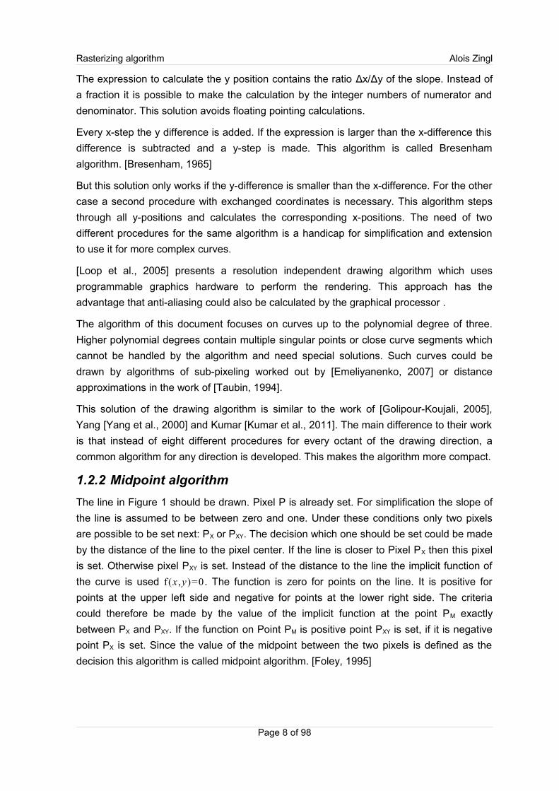
1.2.2 Midpoint algorithm
The line in Figure 1 should be drawn. Pixel P is already set. For simplification the slope of
the line is assumed to be between zero and one. Under these conditions only two pixels
are possible to be set next: PX or PXY. The decision which one should be set could be made
by the distance of the line to the pixel center. If the line is closer to Pixel PX then this pixel
is set. Otherwise pixel PXY is set. Instead of the distance to the line the implicit function of
the curve is used f(x ,y)=0 . The function is zero for points on the line. It is positive for
points at the upper left side and negative for points at the lower right side. The criteria
could therefore be made by the value of the implicit function at the point PM exactly
between PX and PXY. If the function on Point PM is positive point PXY is set, if it is negative
point PX is set. Since the value of the midpoint between the two pixels is defined as the
decision this algorithm is called midpoint algorithm. [Foley, 1995]
Page 8 of 98
Rasterizing algorithm Alois Zingl
Figure 1: Midpoint algorithm
This method is limited to slopes between zero and one. In case of the line a similar
algorithm is needed for slopes above one to decide between the points PXY and PY.
1.2.3 Horner's algorithm
Another way of drawing complex curves is forward differencing by Horner's algorithm
[Foley, 1995]. This algorithm calculates the value of a function just by adding the difference
to the previous value: f(t+Δt) = f(t)+d. If the function is a polynomial of degree one f(t) = a1
t+a0 the difference is only a constant value: d1 = Δt a1. For degree n polynomials the differ-
ences make successive additions: di = di+di+1. The initialization values of di could be calcu-
lated by the differences of the function f(t). If this algorithm is applied on the parametric
equation of the curve x = fx(t) and y = fy(t) the coordinates of Béziers for example could be
calculated only by additions. The problem with this algorithm is to choose an appropriate
step size Δt. If this step is too large a few pixels are omitted and if it is too small the same
pixel is set multiple times.
Horner's algorithm is not limited to lines. It could be used for other curves too. The implicit
function of the curve is needed. Starting at position P every octant of the drawing direction
needs a decision if the pixel in one of the eight appropriate direction should be set or not.
This document somehow applies Horner's algorithm on the implicit equation of the curve.
Another way of rastering a curve is approximation. The curve is subdivided into short lines
and each line is plotted separately. But approximation also means to choose one of two
disadvantages. If the approximation should be accurate the curve must be divided in many
small segments. This is computationally expensive. On the other hand the curve becomes
Page 9 of 98
P
Pxy
Px
f(x,y)=0
PM
Py
Rasterizing algorithm Alois Zingl
edgy if the approximation is not accurate enough. A fast and accurate rasterizing algorithm
for curves is therefore desirable.
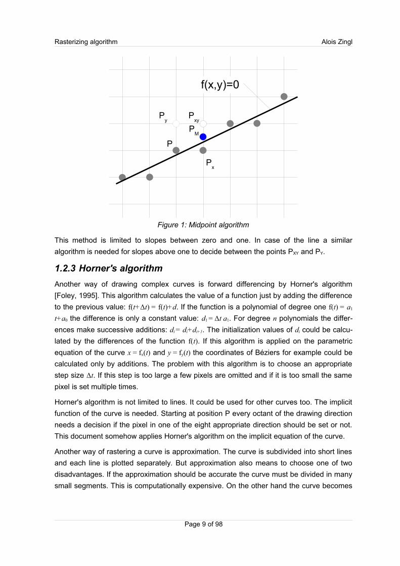
1.3 Problem definition
The implicit equation f(x,y) = 0 defines a curve from the point P0(x0,y0) to P1(x1,y1). The
gradient of the curve must continuously be either positive or negative. This restriction is
solved by subdividing of the curve.
The curve could be a straight line, but also be part of an ellipse or a Bézier curve for
example.
The curve in figure 2 should be digitized into a grid of pixel. This conversion is called
rasterizing.
Which pixel on the grid should be set next to represent the curve in figure 2 most suitably?
1.4 General solution
An error e of the pixel p is introduced by the algorithm as a measurement for the deviation
of the pixel from the curve: e = f(x,y). The error value is zero for pixels exactly at the curve,
positive for one side and negative for the other side of the curve. This error calculation is
Page 10 of 98
Figure 2: Pixel grid of curve f(x,y)=0
p
pxy
px
py
x0,y
0
x1,y
1
f(x,y)=0+
–
Rasterizing algorithm Alois Zingl
used for the decision which pixel should be set next. Starting by pixel p only between three
possible pixel could be chosen for the next pixel because of the positive gradient: PX or
PXY.
The algorithm starts with the assumption that point PXY will be set next. So if the error |exy|
of point PXY is lesser than the error |ex| of pixel PX than the x direction will be incremented.
The same decision is considered for the y direction. If the error |exy| of PXY is lesser than the
error |ey| than the y direction will be incremented. That's why in figure 2 the pixel above P is
labeled PX and besides P is labeled PY.
Since a positive gradient is assumed and the error on one side of the curve will be
negative, the unequation ex ≥ exy ≥ ey will always be true which makes it possible to avoid
the calculation of the absolute value for the comparison. The conditions for the increments
are now:
if ex + exy > 0 then increment x
if ey + exy < 0 then increment y
The benefit of this approach is that the error of the present pixel is already known, so only
the difference to the previous pixel has to be calculated. And this computation is more effi-
cient to implement than calculating the entire expression for every pixel.
The error of the next pixel has to be calculated for all three possibilities of the actual pixel
P: ex, ey and exy. Could that be further reduced? If the algorithm doesn't track the error e of
the current pixel p but the error exy of the next diagonal pixel PXY then only two error calcu-
lations had to be done: ex and ey. Because the error e is not available ex and ey must be
calculated as one pixel less from the actual error.
1.5 Pseudo code of the algorithm
The calculation of the error value depends on the curve function but the condition for the
increment will always be the same.
set up x, y to x0, y0
set up error variable exy for P(x0+1,y0+1)
loop
set pixel x, y
if ex + exy > 0 then increment x, sub difference error
if ey + exy < 0 then increment y, add difference error
loop until end pixel
Listing 1: Pseudo code of the algorithm
Please note that if the condition is true the difference error must be calculated after the
increment is made since the error calculation always looks one diagonal pixel ahead.
Page 11 of 98
Rasterizing algorithm Alois Zingl
A few algorithms in this document contain many details. Not all are explicitly mentioned in
the text. Certain minor implementation solutions could be better and more concisely
explained by sample code. The programming language C is used since it could be easily
converted to other languages. Drawing curves also is a system task and most operating
systems are written in this language. The examples make it also possible to test the
algorithm immediately.
The bit size of the variables is sometimes critical and is assumed to be at least 16 bit for
int, 32 bit for long or float and 64 bit for double.
1.6 Straight lines
The implicit equation for a straight line from point P(x0,y0) to P(x1,y1) is:
(x1–x0)(y–y0)–(x–x0)(y1–y0) = 0 (1)
With the definition of dx = x1–x0 and dy = y1–y0 the error e makes then:
e = (y–y0)dx–(x–x0)dy.
The following calculations are simple but a bit confusing because of the indexes and the
signs.
The error of the diagonal step makes: exy = (y+1–y0)dx–(x+1–x0)dy = e+dx–dy.
The error calculations for the x and y directions make: ex = (y+1–y0)dx–(x–x0)dy = exy+dy and
ey = (y–y0)dx–(x+1–x0)dy = exy–dx.
The error for the first step makes: e1 = (y0+1–y0)dx–(x0+1–x0)dy = dx–dy.
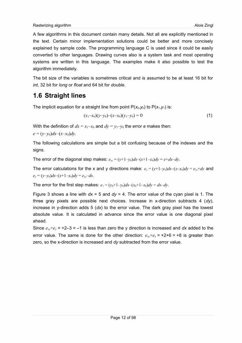
Figure 3 shows a line with dx = 5 and dy = 4. The error value of the cyan pixel is 1. The
three gray pixels are possible next choices. Increase in x-direction subtracts 4 (dy),
increase in y-direction adds 5 (dx) to the error value. The dark gray pixel has the lowest
absolute value. It is calculated in advance since the error value is one diagonal pixel
ahead.
Since exy+ey = +2–3 = –1 is less than zero the y direction is increased and dx added to the
error value. The same is done for the other direction: exy+ex = +2+6 = +8 is greater than
zero, so the x-direction is increased and dy subtracted from the error value.
Page 12 of 98
Rasterizing algorithm Alois Zingl
Although the x and y direction seemed to be interchanged in figure 3 they are actually not.
Just the error increment for the test condition is interchanged.
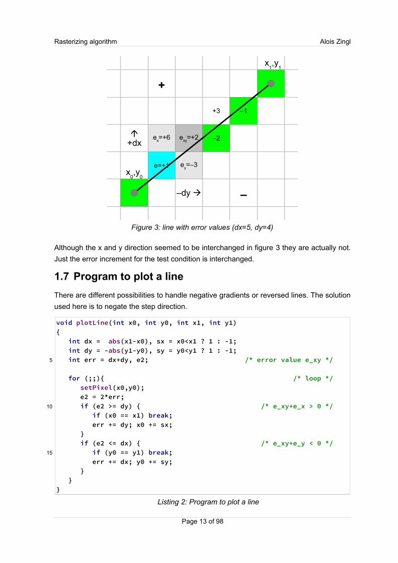
1.7 Program to plot a line
There are different possibilities to handle negative gradients or reversed lines. The solution
used here is to negate the step direction.
void plotLine(int x0, int y0, int x1, int y1){ int dx = abs(x1-x0), sx = x0<x1 ? 1 : -1; int dy = -abs(y1-y0), sy = y0<y1 ? 1 : -1; int err = dx+dy, e2; /* error value e_xy */ for (;;){ /* loop */ setPixel(x0,y0); e2 = 2*err; if (e2 >= dy) { /* e_xy+e_x > 0 */ if (x0 == x1) break; err += dy; x0 += sx; } if (e2 <= dx) { /* e_xy+e_y < 0 */ if (y0 == y1) break; err += dx; y0 += sy; } }}
Listing 2: Program to plot a line
Page 13 of 98
Figure 3: line with error values (dx=5, dy=4)
+3
e=+1
exy
=+2 –2ex=+6
ey=–3
+
–
–1
x0,y
0
x1,y
1
–dy
+dx
5
10
15

Rasterizing algorithm Alois Zingl
There is no approximation by the algorithm. So the error value of the last pixel is always
exactly zero. This version is optimized to check for end-of-the-loop only if the corres-
ponding direction is incremented.
Because this algorithm works in x and y direction symmetrically it needs an additional if
condition in the pixel loop, one more than the traditional Bresenham's line algorithm. It is
possible to avoid this additional condition if it is known in advance that the gradient of the
line is always below or above one.
The program also elegantly illustrates the xy-symmetry of Bresenham's line algorithm. The
same considerations could now be applied to curves of higher polynomial degree.
Due to the symmetry of the line it is also possible to start the drawing form both ends of the
line and stop in the middle. This approach may speed up the drawing but introduces slight
irregularities in the line.
Page 14 of 98
Rasterizing algorithm Alois Zingl
2 Ellipses
Wouldn't it be easier to start with the symmetric circle instead of the more complicated
expression of the ellipse?
It would be, but only a bit. The calculations for ellipses are not so difficult so the solution
can easily be adapted for circles by stetting a = b = r and had not to be done again.
By a proper choice of the coordinate system an ellipse can be described by the implicit
equation: x2b2+y2a2–a2b2 = 0 (2)
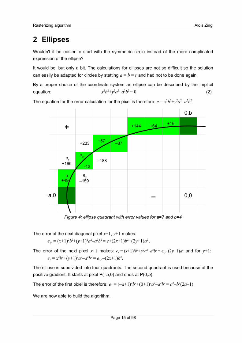
The equation for the error calculation for the pixel is therefore: e = x2b2+y2a2–a2b2.
The error of the next diagonal pixel x+1, y+1 makes:
exy = (x+1)2b2+(y+1)2a2–a2b2 = e+(2x+1)b2+(2y+1)a2 .
The error of the next pixel x+1 makes: ey = (x+1)2b2+y2a2–a2b2 = exy–(2y+1)a2 and for y+1:
ex = x2b2+(y+1)2a2–a2b2 = exy –(2x+1)b2.
The ellipse is subdivided into four quadrants. The second quadrant is used because of the
positive gradient. It starts at pixel P(–a,0) and ends at P(0,b).
The error of the first pixel is therefore: e1 = (–a+1)2b2+(0+1)2a2–a2b2 = a2–b2(2a–1).
We are now able to build the algorithm.
Page 15 of 98
Figure 4: ellipse quadrant with error values for a=7 and b=4
+57
e+49
exy
-12
–87
+144 +64+16
+
––a,0
0,b
0,0
ey
–159
ex
+196 –188
+233
Rasterizing algorithm Alois Zingl
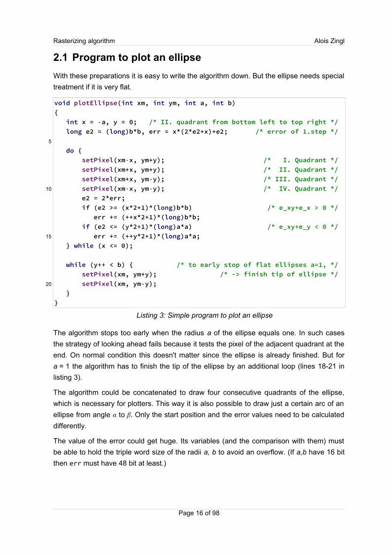
2.1 Program to plot an ellipse
With these preparations it is easy to write the algorithm down. But the ellipse needs special
treatment if it is very flat.
void plotEllipse(int xm, int ym, int a, int b){ int x = -a, y = 0; /* II. quadrant from bottom left to top right */ long e2 = (long)b*b, err = x*(2*e2+x)+e2; /* error of 1.step */ do { setPixel(xm-x, ym+y); /* I. Quadrant */ setPixel(xm+x, ym+y); /* II. Quadrant */ setPixel(xm+x, ym-y); /* III. Quadrant */ setPixel(xm-x, ym-y); /* IV. Quadrant */ e2 = 2*err; if (e2 >= (x*2+1)*(long)b*b) /* e_xy+e_x > 0 */ err += (++x*2+1)*(long)b*b; if (e2 <= (y*2+1)*(long)a*a) /* e_xy+e_y < 0 */ err += (++y*2+1)*(long)a*a; } while (x <= 0); while (y++ < b) { /* to early stop of flat ellipses a=1, */ setPixel(xm, ym+y); /* -> finish tip of ellipse */ setPixel(xm, ym-y); }}
Listing 3: Simple program to plot an ellipse
The algorithm stops too early when the radius a of the ellipse equals one. In such cases
the strategy of looking ahead fails because it tests the pixel of the adjacent quadrant at the
end. On normal condition this doesn't matter since the ellipse is already finished. But for
a = 1 the algorithm has to finish the tip of the ellipse by an additional loop (lines 18-21 in
listing 3).
The algorithm could be concatenated to draw four consecutive quadrants of the ellipse,
which is necessary for plotters. This way it is also possible to draw just a certain arc of an
ellipse from angle α to β. Only the start position and the error values need to be calculated
differently.
The value of the error could get huge. Its variables (and the comparison with them) must
be able to hold the triple word size of the radii a, b to avoid an overflow. (If a,b have 16 bit
then err must have 48 bit at least.)
Page 16 of 98
5
10
15
20
Rasterizing algorithm Alois Zingl
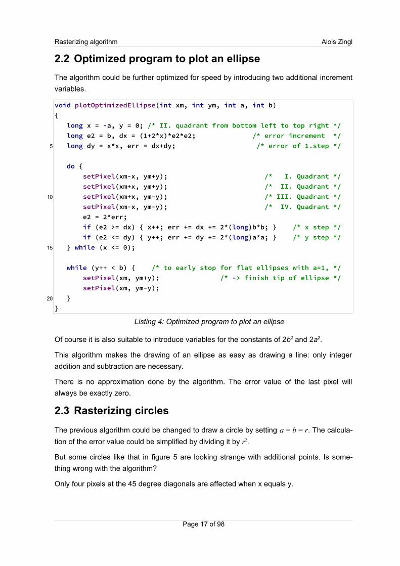
2.2 Optimized program to plot an ellipse
The algorithm could be further optimized for speed by introducing two additional increment
variables.
void plotOptimizedEllipse(int xm, int ym, int a, int b){ long x = -a, y = 0; /* II. quadrant from bottom left to top right */ long e2 = b, dx = (1+2*x)*e2*e2; /* error increment */ long dy = x*x, err = dx+dy; /* error of 1.step */ do { setPixel(xm-x, ym+y); /* I. Quadrant */ setPixel(xm+x, ym+y); /* II. Quadrant */ setPixel(xm+x, ym-y); /* III. Quadrant */ setPixel(xm-x, ym-y); /* IV. Quadrant */ e2 = 2*err; if (e2 >= dx) { x++; err += dx += 2*(long)b*b; } /* x step */ if (e2 <= dy) { y++; err += dy += 2*(long)a*a; } /* y step */ } while (x <= 0); while (y++ < b) { /* to early stop for flat ellipses with a=1, */ setPixel(xm, ym+y); /* -> finish tip of ellipse */ setPixel(xm, ym-y); }}
Listing 4: Optimized program to plot an ellipse
Of course it is also suitable to introduce variables for the constants of 2b2 and 2a2.
This algorithm makes the drawing of an ellipse as easy as drawing a line: only integer
addition and subtraction are necessary.
There is no approximation done by the algorithm. The error value of the last pixel will
always be exactly zero.
2.3 Rasterizing circles
The previous algorithm could be changed to draw a circle by setting a = b = r. The calcula-
tion of the error value could be simplified by dividing it by r2.
But some circles like that in figure 5 are looking strange with additional points. Is some-
thing wrong with the algorithm?
Only four pixels at the 45 degree diagonals are affected when x equals y.
Page 17 of 98
5
10
15
20
Rasterizing algorithm Alois Zingl
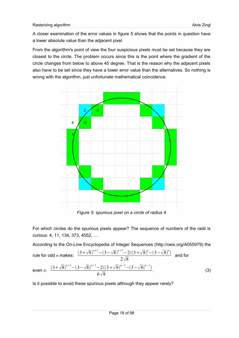
A closer examination of the error values in figure 5 shows that the points in question have
a lower absolute value than the adjacent pixel.
From the algorithm's point of view the four suspicious pixels must be set because they are
closest to the circle. The problem occurs since this is the point where the gradient of the
circle changes from below to above 45 degree. That is the reason why the adjacent pixels
also have to be set since they have a lower error value than the alternatives. So nothing is
wrong with the algorithm, just unfortunate mathematical coincidence.
For which circles do the spurious pixels appear? The sequence of numbers of the radii is
curious: 4, 11, 134, 373, 4552, …
According to the On-Line Encyclopedia of Integer Sequences (http://oeis.org/A055979) the
rule for odd n makes:38
n1−3−8
n1−238
n−3−8
n
28and for
even n:38
n1−3−8
n1−238
n−1−3−8
n−1
68. (3)
Is it possible to avoid these spurious pixels although they appear rarely?
Page 18 of 98
Figure 5: spurious pixel on a circle of radius 4
-32
-3
1
4
Rasterizing algorithm Alois Zingl
One simple way would be by adding the constant value one to the variable err at the initial-
ization making all radii a bit smaller. But this also changes certain other circles, especially
small ones look strange then.
In normal cases these additional pixel will hardly be noticed.
This problem will occur on other curves too.
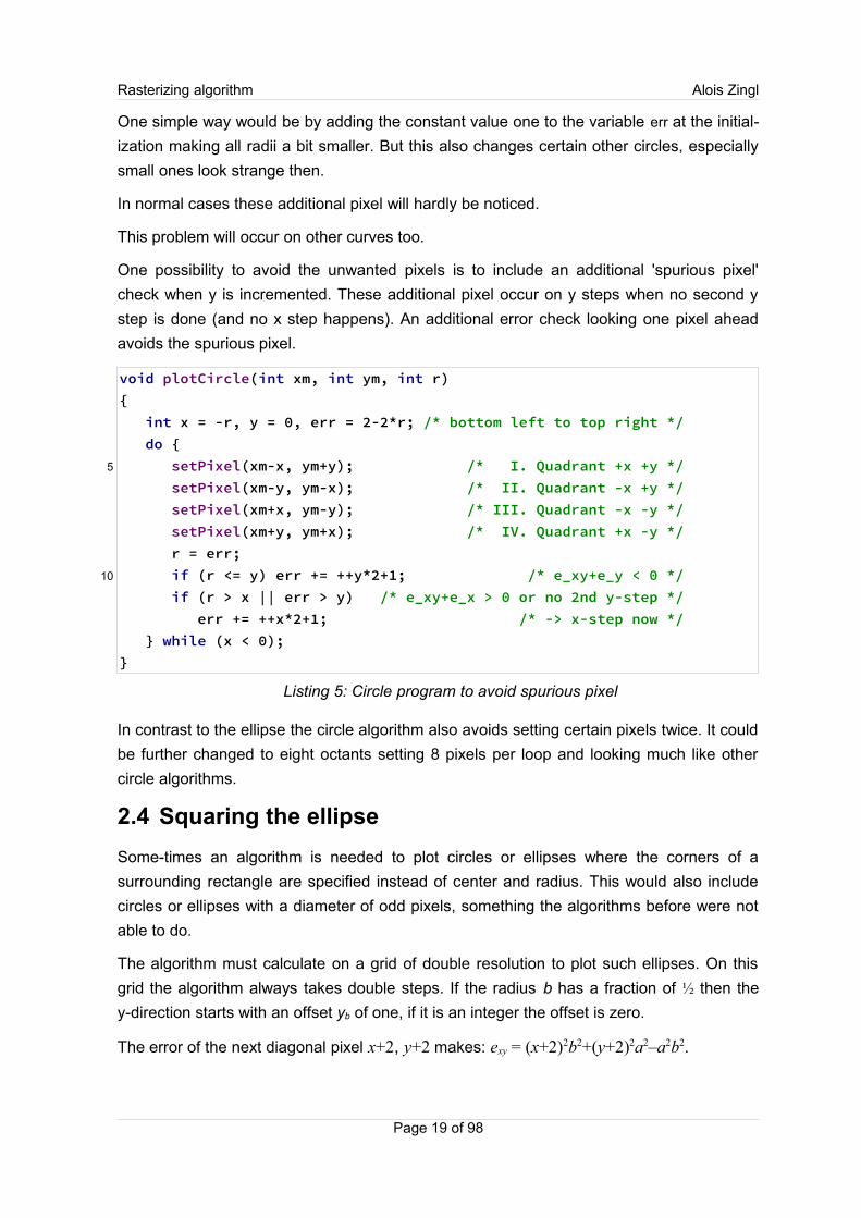
One possibility to avoid the unwanted pixels is to include an additional 'spurious pixel'
check when y is incremented. These additional pixel occur on y steps when no second y
step is done (and no x step happens). An additional error check looking one pixel ahead
avoids the spurious pixel.
void plotCircle(int xm, int ym, int r){ int x = -r, y = 0, err = 2-2*r; /* bottom left to top right */ do { setPixel(xm-x, ym+y); /* I. Quadrant +x +y */ setPixel(xm-y, ym-x); /* II. Quadrant -x +y */ setPixel(xm+x, ym-y); /* III. Quadrant -x -y */ setPixel(xm+y, ym+x); /* IV. Quadrant +x -y */ r = err; if (r <= y) err += ++y*2+1; /* e_xy+e_y < 0 */ if (r > x || err > y) /* e_xy+e_x > 0 or no 2nd y-step */ err += ++x*2+1; /* -> x-step now */ } while (x < 0);}
Listing 5: Circle program to avoid spurious pixel
In contrast to the ellipse the circle algorithm also avoids setting certain pixels twice. It could
be further changed to eight octants setting 8 pixels per loop and looking much like other
circle algorithms.
2.4 Squaring the ellipse
Some-times an algorithm is needed to plot circles or ellipses where the corners of a
surrounding rectangle are specified instead of center and radius. This would also include
circles or ellipses with a diameter of odd pixels, something the algorithms before were not
able to do.
The algorithm must calculate on a grid of double resolution to plot such ellipses. On this
grid the algorithm always takes double steps. If the radius b has a fraction of ½ then the
y-direction starts with an offset yb of one, if it is an integer the offset is zero.
The error of the next diagonal pixel x+2, y+2 makes: exy = (x+2)2b2+(y+2)2a2–a2b2.
Page 19 of 98
5
10
Rasterizing algorithm Alois Zingl
The error of the next pixel x+2 makes: ey = (x+2)2b2+y2a2–a2b2 = exy–4(y+1)a2 and for y+2:
ex = x2b2+(y+2)2a2–a2b2 = exy –4(x+1)b2.
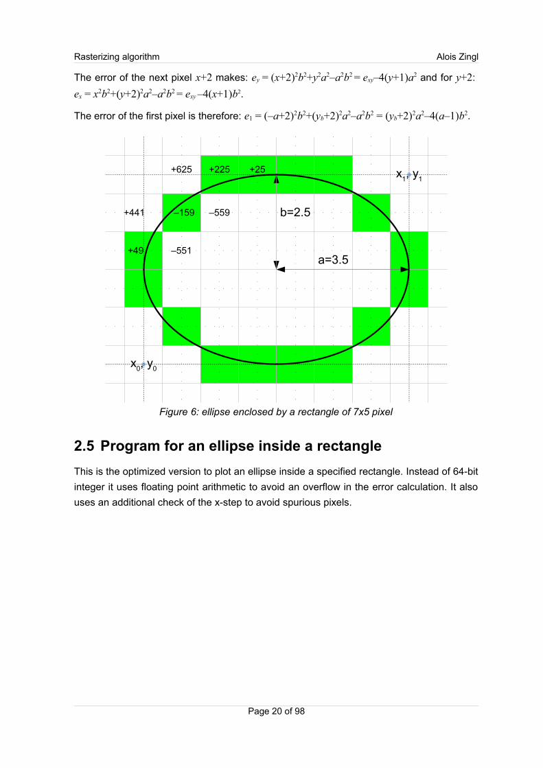
The error of the first pixel is therefore: e1 = (–a+2)2b2+(yb+2)2a2–a2b2 = (yb+2)2a2–4(a–1)b2.
2.5 Program for an ellipse inside a rectangle
This is the optimized version to plot an ellipse inside a specified rectangle. Instead of 64-bit
integer it uses floating point arithmetic to avoid an overflow in the error calculation. It also
uses an additional check of the x-step to avoid spurious pixels.
Page 20 of 98
Figure 6: ellipse enclosed by a rectangle of 7x5 pixel
+25+225
–159
+49
+441
+625
–551
–559
a=3.5
b=2.5
x0, y
0
x1, y
1

Rasterizing algorithm Alois Zingl
void plotEllipseRect(int x0, int y0, int x1, int y1){ /* rectangular parameter enclosing the ellipse */ long a = abs(x1-x0), b = abs(y1-y0), b1 = b&1; /* diameter */ double dx = 4*(1.0-a)*b*b, dy = 4*(b1+1)*a*a; /* error increment */ double err = dx+dy+b1*a*a, e2; /* error of 1.step */
if (x0 > x1) { x0 = x1; x1 += a; } /* if called with swapped points */ if (y0 > y1) y0 = y1; /* .. exchange them */ y0 += (b+1)/2; y1 = y0–b1; /* starting pixel */ a = 8*a*a; b1 = 8*b*b;
do { setPixel(x1, y0); /* I. Quadrant */ setPixel(x0, y0); /* II. Quadrant */ setPixel(x0, y1); /* III. Quadrant */ setPixel(x1, y1); /* IV. Quadrant */ e2 = 2*err; if (e2 <= dy) { y0++; y1--; err += dy += a; } /* y step */ if (e2 >= dx || 2*err > dy) { x0++; x1--; err += dx += b1;} /* x */ } while (x0 <= x1);
while (y0-y1 <= b) { /* to early stop of flat ellipses a=1 */ setPixel(x0-1, y0); /* -> finish tip of ellipse */ setPixel(x1+1, y0++); setPixel(x0-1, y1); setPixel(x1+1, y1--); }}
Listing 6: Program to plot an ellipse enclosed by a rectangle
This algorithm works for all values of x0, y0, x1 and y1.
The algorithm for rotated ellipses is developed later since the direct drawing algorithm runs
into troubles but could be implemented by using rational Béziers.
Page 21 of 98
5
10
15
20
25

Rasterizing algorithm Alois Zingl
3 Quadratic Bézier curves
The concept of universal curves were independently developed by the French engineers
Pierre Étienne Bezier from Renault and Paul de Faget de Casteljau from Citroën at the
advent of the computer aided manufacturing in the car industry to design automobile
bodies. [Bézier, 1986] [Casteljau, 1963]
Bézier curves consist of a set of control points. The number of points define the order of
the curve.
The general Bézier equation of order n in parametric form given n +1 points Pi is defined to
be [Marsh, 2005, p. 135]
(4)
This is a straight line for order n = 1. For order n = 2 this is the quadratic Bézier curve
B2t =1−t 2 P02 1−t t P1t 2 P2. (5)
The conical implicit equation of the Bézier curve is needed for the algorithm.
The general implicit equation of degree 2 makes:
A x22 B x yC y2
2 D x2 E yF=0.
This equation has six unknown coefficients so six linearly independent equations are
needed to derive the unknowns. If F is non zero the equation could be divided by F:
a x22b x yc y2
2d x2e y1=0 leaving five unknowns.
Two could be derived by setting x = x0 → y = y0 and x = x2 → y = y2:
a x022 b x0 y0c y0
22 d x02 e y0=−1 and a x2
22b x2 y2c y2
22 d x22 e y2=−1.
Page 22 of 98
Figure 7: Bézier curve of degree 2
P0
P1
P2
Bn t =∑i=0
n
ni 1−t n−i ti P i

Rasterizing algorithm Alois Zingl
A third could be derived from the parametric form by setting t = ½:
B212 =P02P1P2
4
a x02 x1 x222b x02 x1 x2 y02 y1 y2c y02 y1 y2
2... (6)
...8d x02 x1 x28e y02 y1 y2=−16
The last two unknowns are computed by the derivative of the implicit equation:
∇ x , y=⟨2 a x2b y2 d ,2b x2c y2e ⟩
By the gradients at the two points P0:x0−x1
y0− y1
=a x0b y0d
b x0c y0eand P2:
x2−x1
y2− y1
=a x2b y2d
b x2c y2ethe equations for the last two unknowns could be derived:
a x0x0− x1b y0x0− x1 x0 y0− y1c y0 y0− y1d x0− x1e y0− y1=0
a x2x2−x1b y2x2−x1 x2 y2− y1c y2 y2− y1d x2−x1e y2− y1=0
The computations of the unknowns get a bit difficult now. Could they be simplified? By the
substitution of P i=Pi−P1 the Bézier curve is shifted by the offset of –P1. It is no problem
for the algorithm to shift it back later. So for the simplification of this computation point P1 is
assumed to be at the origin: x1=y1=0 and the values of x1 and y1 are subtracted from
the other points: x i= x i−x1 . The system of five linear equations could now be written as
the matrix equation
[x0
2 2 x0 y0 y02 2 x0 2 y0
x22 2 x2 y2 y2
2 2 x2 2 y2
x0x22 2 x0x2 y0y2 y0 y 2
2 8 x0x 2 8 y0y2
x02 2 x0 y0 y0
2x0 y0
x22 2 x2 y2 y2
2x2 y2
]⋅[abcde]=[−1−1−16
00] (7)
This matrix equation can be solved like below:
A= y0 y 22 ,B=− x0x2 y0y2 ,C=x0x2
2 ,
D= y0− y2 x0 y2−x2 y0 , E=− x0−x2 x0 y2−x2 y0 , F= x0 y2−x2 y02 .
The implicit equation of the quadratic Bézier curve for x1=y1=0 makes:
x2 y0y2
2−2 x y x0x 2 y0y2 y2
y0 y22
2x y0− y2− y x0−x2 x0 y2−x2 y0 x0 y2−x2 y02=0.
The overall curvature of the Bézier curve is defined by
cur=x0 y2−x2 y0=x0− x1 y2− y1−x2−x1 y0− y1 . (8)
The previous substitutions could be added again. By some computations the implicit equa-
tion of the quadratic Bézier curve is simplified to:
Page 23 of 98
Rasterizing algorithm Alois Zingl
(x ( y0−2 y1+ y2)− y( x0−2 x1+ x2))2+2(x ( y0− y 2)− y ( x0−x2))cur+cur 2=0. (9)
The quadratic Bézier curve is part of a parabola.
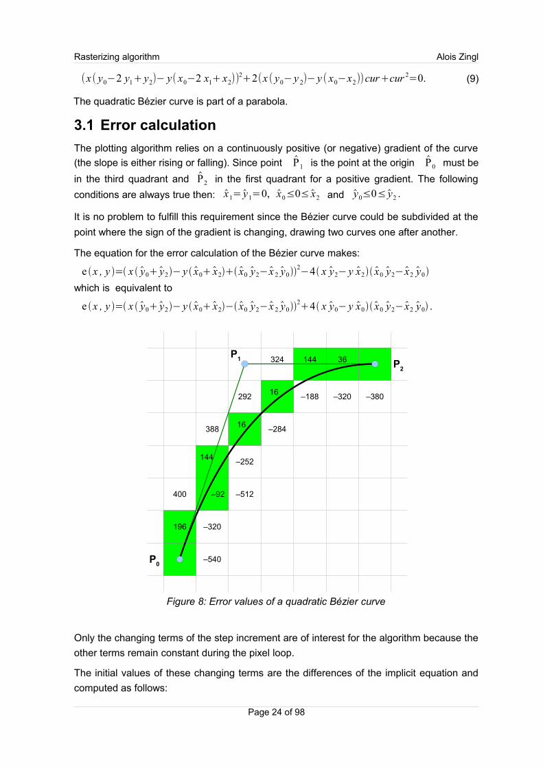
3.1 Error calculation
The plotting algorithm relies on a continuously positive (or negative) gradient of the curve
(the slope is either rising or falling). Since point P1 is the point at the origin P0 must be
in the third quadrant and P2 in the first quadrant for a positive gradient. The following
conditions are always true then: x1=y1=0, x0≤0≤x2 and y0≤0≤y2 .
It is no problem to fulfill this requirement since the Bézier curve could be subdivided at the
point where the sign of the gradient is changing, drawing two curves one after another.
The equation for the error calculation of the Bézier curve makes:
e x , y = x y0y2− y x0x2 x0 y2−x 2 y02−4 x y2− y x2 x0 y2−x2 y0
which is equivalent to
e x , y = x y0y2− y x0x2− x0 y2−x 2 y024 x y0− y x0 x0 y2−x2 y0 .
Figure 8: Error values of a quadratic Bézier curve
Only the changing terms of the step increment are of interest for the algorithm because the
other terms remain constant during the pixel loop.
The initial values of these changing terms are the differences of the implicit equation and
computed as follows:
Page 24 of 98
36144
16
16
144
–92
196 –320
400
–252
388
–540
–512
–284
292 –188
324
–320 –380
P0
P1
P2
Rasterizing algorithm Alois Zingl
d x=e x±1, y −e x , y =1±2 x y0y22∓2 y x0x2 y0y2±2cur y0−y2 ,
d y=e x , y±1−e x , y =1±2 y x0x22∓2 x x0x2 y0 y 2∓2cur x0−x2.
Since this Bézier curve is of second degree the increment error changes each step too.
Not only the error of the calculation has to be incremented according to the steps, but also
the increment of dx and dy itself changes each step. In case of a quadratic polynomial this
could also be computed by the second derivative.
For the step in x-direction the increment dx is increased about
d xx=e x2, y−2e x1, y=∂
2e∂ x2=2 y0y2
2=2 y0−2 y1 y2
2and dy is increased
aboutd xy=e x1, y1−ex1, y −e x , y1=
∂2 e
∂ x∂ y=−2 x0x2 y0 y2=
=−2 x0−2 x1x2 y0−2 y1 y2.
For the step in y-direction the increment dy is increased about
d yy=e x , y2−2 e x , y1=∂
2e∂ y2=2 x0x2
2=2 x0−2 x1 x2
2
and dx is increased about∂
2e∂ x ∂ y
.
These increments are independent of x and y.
3.2 Troubles with slightly curved linesSo far the algorithm seems to work out nicely. But it fails when the Bézier curve becomes
nearly a straight line. What happens becomes clear if the entire curve is analyzed, not only
the short part the algorithm wants to plot. The curve is a symmetric parabola. It has a
second part. For curves with large curvature the second half is far away, leaving a clear
path the algorithm can follow. But on nearly straight lines this second half can fall within the
current possible pixel! Then the algorithm is confused since it relies on a clear gradient of
error values.
This problem occurred before. On flat ellipses with a = 1 the algorithm stopped to early. But
the situation was lucky. The ellipses were always placed in symmetric orthogonal
orientation. The algorithm failed only in one case which could be fixed by an extra loop.
Page 25 of 98
Rasterizing algorithm Alois Zingl
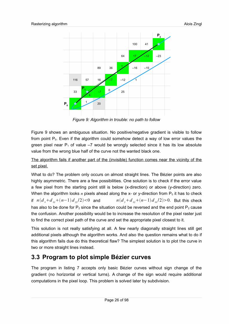
Figure 9 shows an ambiguous situation. No positive/negative gradient is visible to follow
from point P0. Even if the algorithm could somehow detect a way of low error values the
green pixel near P1 of value –7 would be wrongly selected since it has its low absolute
value from the wrong blue half of the curve not the wanted black one.
T he al gorithm fails if another part of the (invisible) function comes near the vicinity of the
set pixel.
What to do? The problem only occurs on almost straight lines. The Bézier points are also
highly asymmetric. There are a few possibilities. One solution is to check if the error value
a few pixel from the starting point still is below (x-direction) or above (y-direction) zero.
When the algorithm looks n pixels ahead along the x- or y-direction from P0 it has to check
if n d xd xyn−1d yy /20 and n d yd xyn−1d xx /20. But this check
has also to be done for P2 since the situation could be reversed and the end point P2 cause
the confusion. Another possibility would be to increase the resolution of the pixel raster just
to find the correct pixel path of the curve and set the appropriate pixel closest to it.
This solution is not really satisfying at all. A few nearly diagonally straight lines still get
additional pixels although the algorithm works. And also the question remains what to do if
this algorithm fails due do this theoretical flaw? The simplest solution is to plot the curve in
two or more straight lines instead.
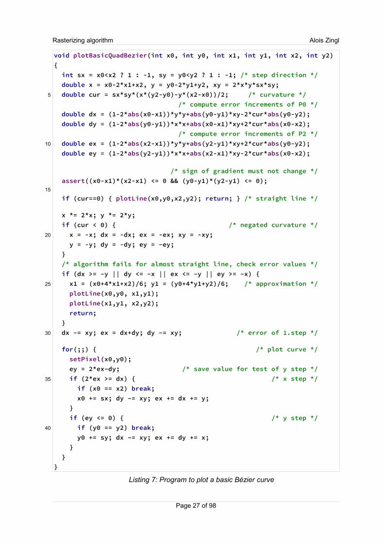
3.3 Program to plot simple Bézier curves
The program in listing 7 accepts only basic Bézier curves without sign change of the
gradient (no horizontal or vertical turns). A change of the sign would require additional
computations in the pixel loop. This problem is solved later by subdivision.
Page 26 of 98
Figure 9: Algorithm in trouble: no path to follow
20
116
–1217
1
–7
–7 4
330
36
1
16 –1257
–16
100
1
41
P0
P1
P2
–15
–23
25
64
89
Rasterizing algorithm Alois Zingl
void plotBasicQuadBezier(int x0, int y0, int x1, int y1, int x2, int y2){ int sx = x0<x2 ? 1 : -1, sy = y0<y2 ? 1 : -1; /* step direction */ double x = x0-2*x1+x2, y = y0-2*y1+y2, xy = 2*x*y*sx*sy; double cur = sx*sy*(x*(y2-y0)-y*(x2-x0))/2; /* curvature */ /* compute error increments of P0 */ double dx = (1-2*abs(x0-x1))*y*y+abs(y0-y1)*xy-2*cur*abs(y0-y2); double dy = (1-2*abs(y0-y1))*x*x+abs(x0-x1)*xy+2*cur*abs(x0-x2); /* compute error increments of P2 */ double ex = (1-2*abs(x2-x1))*y*y+abs(y2-y1)*xy+2*cur*abs(y0-y2); double ey = (1-2*abs(y2-y1))*x*x+abs(x2-x1)*xy-2*cur*abs(x0-x2);
/* sign of gradient must not change */ assert((x0-x1)*(x2-x1) <= 0 && (y0-y1)*(y2-y1) <= 0);
if (cur==0) { plotLine(x0,y0,x2,y2); return; } /* straight line */
x *= 2*x; y *= 2*y; if (cur < 0) { /* negated curvature */ x = -x; dx = -dx; ex = -ex; xy = -xy; y = -y; dy = -dy; ey = –ey; } /* algorithm fails for almost straight line, check error values */ if (dx >= –y || dy <= –x || ex <= –y || ey >= –x) { x1 = (x0+4*x1+x2)/6; y1 = (y0+4*y1+y2)/6; /* approximation */ plotLine(x0,y0, x1,y1); plotLine(x1,y1, x2,y2); return; } dx –= xy; ex = dx+dy; dy –= xy; /* error of 1.step */
for(;;) { /* plot curve */ setPixel(x0,y0); ey = 2*ex–dy; /* save value for test of y step */ if (2*ex >= dx) { /* x step */ if (x0 == x2) break; x0 += sx; dy –= xy; ex += dx += y; } if (ey <= 0) { /* y step */ if (y0 == y2) break; y0 += sy; dx –= xy; ex += dy += x; } }}
Listing 7: Program to plot a basic Bézier curve
Page 27 of 98
5
10
15
20
25
30
35
40
Rasterizing algorithm Alois Zingl
A few comments to listing 7:
A negative curvature negates the gradient of the error values. This leaves the possibility to
either negate the other values too or use another pixel loop with interchanged condition
(exy+dx<0 → x++).
The error increments are used to look three pixel in x and y-direction ahead and detect
almost straight lines by an additional gradient change of the error values. This is done for
both ends at which the increments of P2 are only needed for this check. The curve is drawn
by two lines in this case.
There is no approximation done by the curve algorithm. The error value of the last pixel will
always be exactly zero. That's why the break condition of the loop is secure to test just for
the last pixel. But during testing it is helpful to add an additional loop counter in the for
statement if something goes wrong.
Since each step also modifies the increment value it had to be saved for the second test.
Otherwise a few pixel would shift one y-step. This would normally not be noticed except if
this was the last pixel for the test of the break condition.
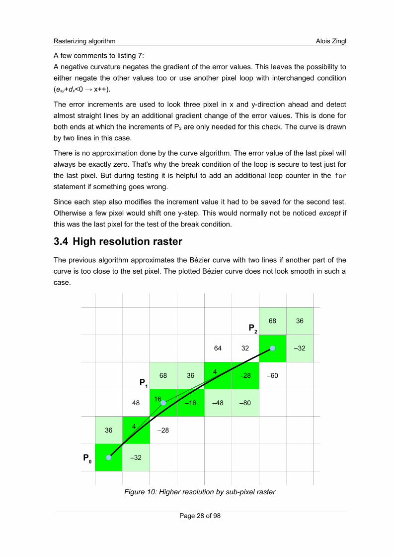
3.4 High resolution raster
The previous algorithm approximates the Bézier curve with two lines if another part of the
curve is too close to the set pixel. The plotted Bézier curve does not look smooth in such a
case.
Page 28 of 98
Figure 10: Higher resolution by sub-pixel raster
4 36
16
4 36
68
–32
–16 –48 –80
–32
3668
32
–28
48
–28
64
P0
P1
P2
–60
Rasterizing algorithm Alois Zingl
Another alternative is to use a finer raster of sub-pixel and set the pixel closest to this pixel
curve. This high resolution raster must be sufficiently fine to avoid a conflict of two curves
on one pixel or very close pixel.
Figure 10 shows a Bézier curve with a sub-pixel raster of double precision. Each pixel
(light-green) is divided in sub-pixel (green).
The algorithm itself works on the finer pixel raster and has therefore no problem finding a
path of suitable error values. Every time a sub-pixel is complete the pixel itself is set.
The concept of sub-pixeling is also used by the algorithm of [Emeliyanenko, 2007] to
exactly draw implicit curves. This concept offers a solution if the algorithm of this document
fails or gets too complicated for an implementation.
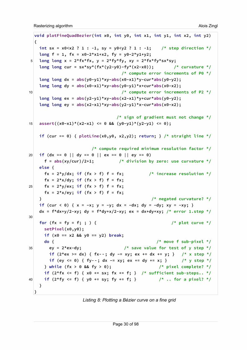
The version in listing 8 requires more computations in the pixel loop than the basic
algorithm and is therefore a bit slower but never approximates the quadratic Bézier curve.
The calculation of the resolution factor makes sure that the sign of the error value does not
change due to a close curve three sub-pixel from P0 or P2 in x or y direction. But this solu-
tion ends in a division-by-zero in case of a maximum which has to be given special care.
Since the error calculation is one pixel ahead, the computation of the last step goes
beyond the end pixel. The basic algorithm has no problem stopping in this case although
the increment values may already be invalid since the curve could make a sharp turn. But
the fine algorithm finishes all sub-pixels of a pixel. But in case of a turn the sub-pixels
cannot be finished since the increment values already changed the sign. For this case an
extra break condition must be inserted in the inner loop to avoid an infinite loop.
This resolution factor can get quite large for certain Béziers. But only a few eccentric
curves slow the algorithm down.
The benefit of this algorithm is that the plotted curve has no approximation errors. All set
pixels are as close as possible to the analog Bézier curve.
An option is to use the fine algorithm only if the basic version fails (f >1). A long curve
could also be subdivided into a long nearly straight part plotted by the faster basic version
and a shorter curved part by the fine algorithm.
Page 29 of 98
Rasterizing algorithm Alois Zingl
void plotFineQuadBezier(int x0, int y0, int x1, int y1, int x2, int y2){ int sx = x0<x2 ? 1 : -1, sy = y0<y2 ? 1 : -1; /* step direction */ long f = 1, fx = x0–2*x1+x2, fy = y0–2*y1+y2; long long x = 2*fx*fx, y = 2*fy*fy, xy = 2*fx*fy*sx*sy; long long cur = sx*sy*(fx*(y2–y0)–fy*(x2–x0)); /* curvature */ /* compute error increments of P0 */ long long dx = abs(y0–y1)*xy–abs(x0–x1)*y–cur*abs(y0–y2); long long dy = abs(x0–x1)*xy–abs(y0–y1)*x+cur*abs(x0–x2); /* compute error increments of P2 */ long long ex = abs(y2–y1)*xy–abs(x2–x1)*y+cur*abs(y0–y2); long long ey = abs(x2–x1)*xy–abs(y2–y1)*x–cur*abs(x0–x2); /* sign of gradient must not change */ assert((x0–x1)*(x2–x1) <= 0 && (y0–y1)*(y2–y1) <= 0);
if (cur == 0) { plotLine(x0,y0, x2,y2); return; } /* straight line */
/* compute required minimum resolution factor */ if (dx == 0 || dy == 0 || ex == 0 || ey == 0) f = abs(xy/cur)/2+1; /* division by zero: use curvature */ else { fx = 2*y/dx; if (fx > f) f = fx; /* increase resolution */ fx = 2*x/dy; if (fx > f) f = fx; fx = 2*y/ex; if (fx > f) f = fx; fx = 2*x/ey; if (fx > f) f = fx; } /* negated curvature? */ if (cur < 0) { x = –x; y = –y; dx = –dx; dy = –dy; xy = –xy; } dx = f*dx+y/2–xy; dy = f*dy+x/2–xy; ex = dx+dy+xy; /* error 1.step */
for (fx = fy = f; ; ) { /* plot curve */ setPixel(x0,y0); if (x0 == x2 && y0 == y2) break; do { /* move f sub-pixel */ ey = 2*ex–dy; /* save value for test of y step */ if (2*ex >= dx) { fx--; dy –= xy; ex += dx += y; } /* x step */ if (ey <= 0) { fy--; dx –= xy; ex += dy += x; } /* y step */ } while (fx > 0 && fy > 0); /* pixel complete? */ if (2*fx <= f) { x0 += sx; fx += f; } /* sufficient sub-steps.. */ if (2*fy <= f) { y0 += sy; fy += f; } /* .. for a pixel? */ }}
Listing 8: Plotting a Bézier curve on a fine grid
Page 30 of 98
5
10
15
20
25
30
35
40
Rasterizing algorithm Alois Zingl
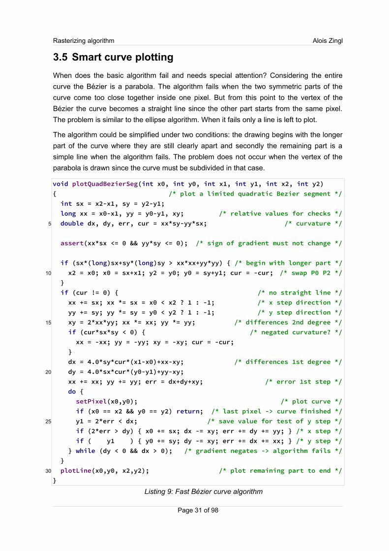
3.5 Smart curve plotting
When does the basic algorithm fail and needs special attention? Considering the entire
curve the Bézier is a parabola. The algorithm fails when the two symmetric parts of the
curve come too close together inside one pixel. But from this point to the vertex of the
Bézier the curve becomes a straight line since the other part starts from the same pixel.
The problem is similar to the ellipse algorithm. When it fails only a line is left to plot.
The algorithm could be simplified under two conditions: the drawing begins with the longer
part of the curve where they are still clearly apart and secondly the remaining part is a
simple line when the algorithm fails. The problem does not occur when the vertex of the
parabola is drawn since the curve must be subdivided in that case.
void plotQuadBezierSeg(int x0, int y0, int x1, int y1, int x2, int y2){ /* plot a limited quadratic Bezier segment */ int sx = x2-x1, sy = y2-y1; long xx = x0-x1, yy = y0-y1, xy; /* relative values for checks */ double dx, dy, err, cur = xx*sy-yy*sx; /* curvature */
assert(xx*sx <= 0 && yy*sy <= 0); /* sign of gradient must not change */
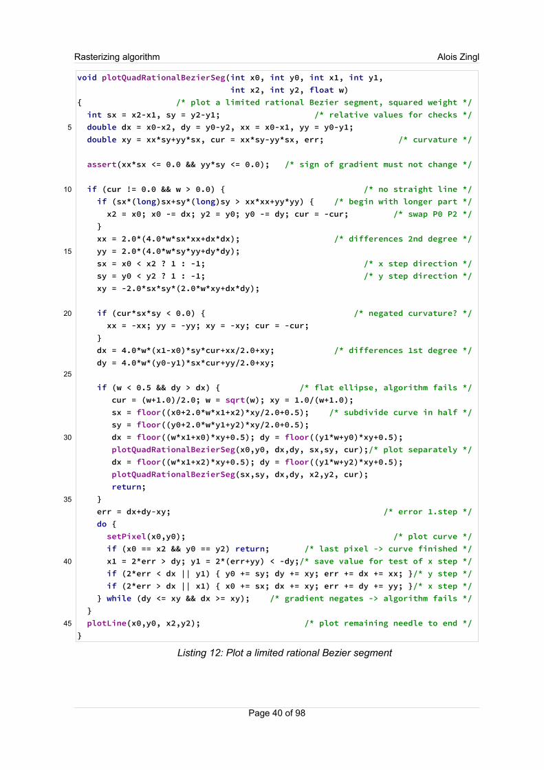
if (sx*(long)sx+sy*(long)sy > xx*xx+yy*yy) { /* begin with longer part */ x2 = x0; x0 = sx+x1; y2 = y0; y0 = sy+y1; cur = -cur; /* swap P0 P2 */ } if (cur != 0) { /* no straight line */ xx += sx; xx *= sx = x0 < x2 ? 1 : -1; /* x step direction */ yy += sy; yy *= sy = y0 < y2 ? 1 : -1; /* y step direction */ xy = 2*xx*yy; xx *= xx; yy *= yy; /* differences 2nd degree */ if (cur*sx*sy < 0) { /* negated curvature? */ xx = -xx; yy = -yy; xy = -xy; cur = -cur; } dx = 4.0*sy*cur*(x1-x0)+xx-xy; /* differences 1st degree */ dy = 4.0*sx*cur*(y0-y1)+yy-xy; xx += xx; yy += yy; err = dx+dy+xy; /* error 1st step */ do { setPixel(x0,y0); /* plot curve */ if (x0 == x2 && y0 == y2) return; /* last pixel -> curve finished */ y1 = 2*err < dx; /* save value for test of y step */ if (2*err > dy) { x0 += sx; dx -= xy; err += dy += yy; } /* x step */ if ( y1 ) { y0 += sy; dy -= xy; err += dx += xx; } /* y step */ } while (dy < 0 && dx > 0); /* gradient negates -> algorithm fails */ } plotLine(x0,y0, x2,y2); /* plot remaining part to end */}
Listing 9: Fast Bézier curve algorithm
Page 31 of 98
5
10
15
20
25
30
Rasterizing algorithm Alois Zingl
The algorithm begins at the end which is farther away from the vertex since the other part
of the curve is then probably far enough away. The algorithm stops if the two symmetric
parts of the parabola come too close together and the algorithm fails. This could be tested
if the derivative of the gradient of the error value changes its sign. The curve is then
finished by plotting a straight line to the end of the curve.
The problem does not occur when the Bézier curve consists of both parts of the parabola.
If the curvature of the vertex shrinks to a single point then the curve must be subdivided
before since the gradient also changes the direction there. If it is not a single point then the
two sides are far enough apart and the algorithm does not fail.
This solution is very efficient to plot a quadratic Bézier curve. The algorithm has the
advantage that if the curve comes too close together to work it is straight enough to be
finished by a line so it never fails.
Since the error values can get quite large (up to the fourth power) the double type is used
instead of a long integer. If a 64-bit integer type is available this type could be used
instead.
3.6 Common Bézier curves
The previous Bézier algorithms rely on a continuously positive or negative gradient to keep
it simple. A sign change would imply a change in the direction of the set pixel inside the
loop. The error calculation is one pixel ahead and would need a change too. The Bézier
curve is subdivided at the horizontal and vertical turns to avoid these troubles.
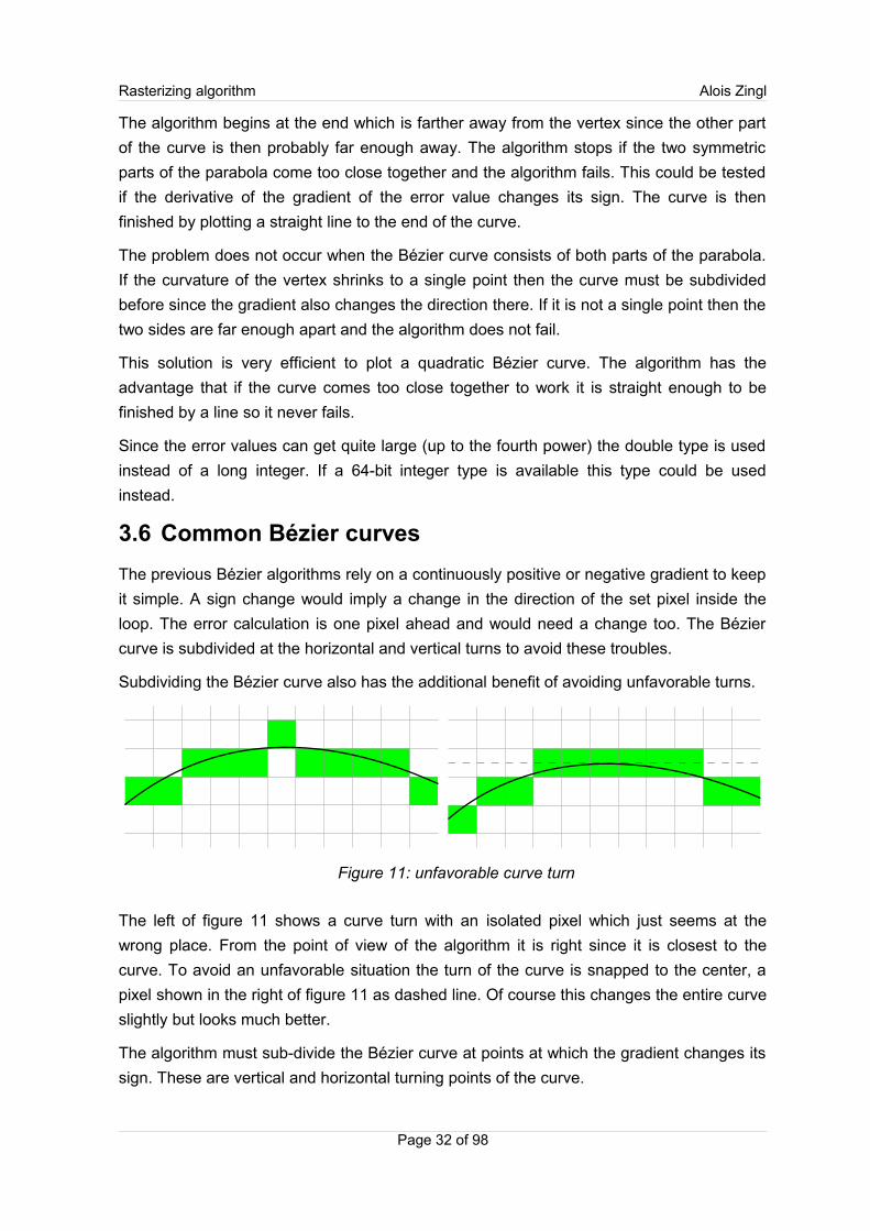
Subdividing the Bézier curve also has the additional benefit of avoiding unfavorable turns.
Figure 11: unfavorable curve turn
The left of figure 11 shows a curve turn with an isolated pixel which just seems at the
wrong place. From the point of view of the algorithm it is right since it is closest to the
curve. To avoid an unfavorable situation the turn of the curve is snapped to the center, a
pixel shown in the right of figure 11 as dashed line. Of course this changes the entire curve
slightly but looks much better.
The algorithm must sub-divide the Bézier curve at points at which the gradient changes its
sign. These are vertical and horizontal turning points of the curve.
Page 32 of 98
Rasterizing algorithm Alois Zingl
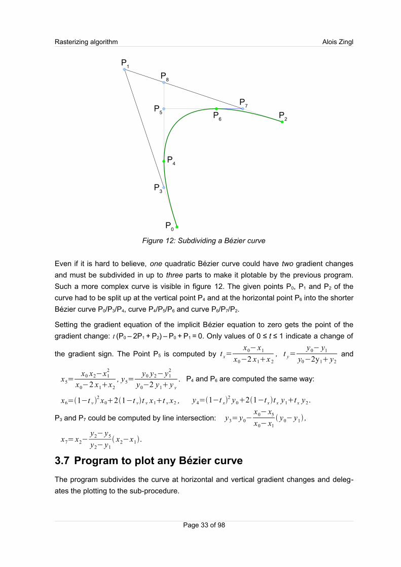
Even if it is hard to believe, one quadratic Bézier curve could have two gradient changes
and must be subdivided in up to three parts to make it plotable by the previous program.
Such a more complex curve is visible in figure 12. The given points P0, P1 and P2 of the
curve had to be split up at the vertical point P4 and at the horizontal point P6 into the shorter
Bézier curve P0/P3/P4, curve P4/P5/P6 and curve P6/P7/P2.
Setting the gradient equation of the implicit Bézier equation to zero gets the point of the
gradient change: t (P0 – 2P1 + P2) – P0 + P1 = 0. Only values of 0 ≤ t ≤ 1 indicate a change of
the gradient sign. The Point P5 is computed by t x=x0− x1
x0−2 x1x 2
, t y=y0− y1
y0−2y1 y2
and
x5=x0 x2−x1
2
x0−2 x1x2
, y5=y0 y2− y1
2
y0−2 y1 y y
. P4 and P6 are computed the same way:
x6=1−t y 2 x021−t yt y x1t y x2 , y4=1−t x
2 y021−t x t x y1t x y2.
P3 and P7 could be computed by line intersection: y3= y0−x0− x5
x0− x1
y0− y1 ,
x7= x2−y2− y5
y2− y1
x2−x1.
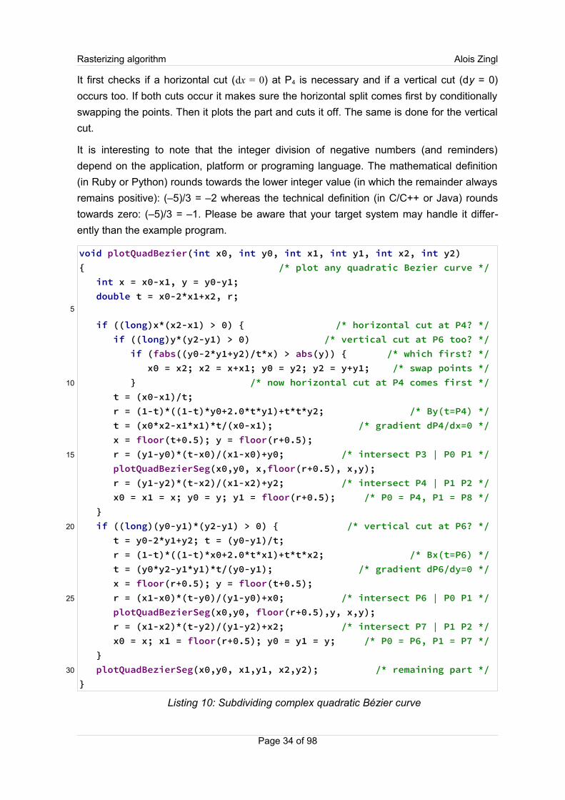
3.7 Program to plot any Bézier curve
The program subdivides the curve at horizontal and vertical gradient changes and deleg-
ates the plotting to the sub-procedure.
Page 33 of 98
Figure 12: Subdividing a Bézier curve
P0
P1
P2
P5
P4
P3
P6
P7
P8
Rasterizing algorithm Alois Zingl
It first checks if a horizontal cut (dx = 0) at P4 is necessary and if a vertical cut (dy = 0)
occurs too. If both cuts occur it makes sure the horizontal split comes first by conditionally
swapping the points. Then it plots the part and cuts it off. The same is done for the vertical
cut.
It is interesting to note that the integer division of negative numbers (and reminders)
depend on the application, platform or programing language. The mathematical definition
(in Ruby or Python) rounds towards the lower integer value (in which the remainder always
remains positive): (–5)/3 = –2 whereas the technical definition (in C/C++ or Java) rounds
towards zero: (–5)/3 = –1. Please be aware that your target system may handle it differ-
ently than the example program.
void plotQuadBezier(int x0, int y0, int x1, int y1, int x2, int y2){ /* plot any quadratic Bezier curve */ int x = x0-x1, y = y0-y1; double t = x0-2*x1+x2, r;
if ((long)x*(x2-x1) > 0) { /* horizontal cut at P4? */ if ((long)y*(y2-y1) > 0) /* vertical cut at P6 too? */ if (fabs((y0-2*y1+y2)/t*x) > abs(y)) { /* which first? */ x0 = x2; x2 = x+x1; y0 = y2; y2 = y+y1; /* swap points */ } /* now horizontal cut at P4 comes first */ t = (x0-x1)/t; r = (1-t)*((1-t)*y0+2.0*t*y1)+t*t*y2; /* By(t=P4) */ t = (x0*x2-x1*x1)*t/(x0-x1); /* gradient dP4/dx=0 */ x = floor(t+0.5); y = floor(r+0.5); r = (y1-y0)*(t-x0)/(x1-x0)+y0; /* intersect P3 | P0 P1 */ plotQuadBezierSeg(x0,y0, x,floor(r+0.5), x,y); r = (y1-y2)*(t-x2)/(x1-x2)+y2; /* intersect P4 | P1 P2 */ x0 = x1 = x; y0 = y; y1 = floor(r+0.5); /* P0 = P4, P1 = P8 */ } if ((long)(y0-y1)*(y2-y1) > 0) { /* vertical cut at P6? */ t = y0-2*y1+y2; t = (y0-y1)/t; r = (1-t)*((1-t)*x0+2.0*t*x1)+t*t*x2; /* Bx(t=P6) */ t = (y0*y2-y1*y1)*t/(y0-y1); /* gradient dP6/dy=0 */ x = floor(r+0.5); y = floor(t+0.5); r = (x1-x0)*(t-y0)/(y1-y0)+x0; /* intersect P6 | P0 P1 */ plotQuadBezierSeg(x0,y0, floor(r+0.5),y, x,y); r = (x1-x2)*(t-y2)/(y1-y2)+x2; /* intersect P7 | P1 P2 */ x0 = x; x1 = floor(r+0.5); y0 = y1 = y; /* P0 = P6, P1 = P7 */ } plotQuadBezierSeg(x0,y0, x1,y1, x2,y2); /* remaining part */}
Listing 10: Subdividing complex quadratic Bézier curve
Page 34 of 98
5
10
15
20
25
30
Rasterizing algorithm Alois Zingl
Rounding in C is a bit tricky especially if it should also work for negative numbers. Floating
point arithmetic is therefore only used for proper rounding of the divisions. It is also
possible to do it in integers only but it is more complicated:
round(a/b) = (a+sign(a)*abs(b)/2)/b.
Sub dividing a Bézier curve always leads to certain integer rounding errors of the Bézier
points. This becomes especially visible if two of the points of a Bézier come close together
(about < 10 pixel). Sometimes one of the curves even becomes a straight line and does
not seem to fit to the others. On the other hand this also has the benefit that horizontal
and/or vertical intervals of the curve are always rasterized on full pixel. Curved transitions
look much better that way.
The middle control point P1 could be changed to a thru point P1 by P1=2 P1−P0P2
2. (10)
Page 35 of 98
Rasterizing algorithm Alois Zingl
4 Rational Béziers
For rational Béziers each point Pi of equation (4) gets an additional weight wi: [Marsh,
2005, p. 175]
Bn t =∑
ini 1−t n−i t i wi Pi
∑ini 1−t n−i t i w i
. [ 0 ≤ t ≤ 1 ] (11)
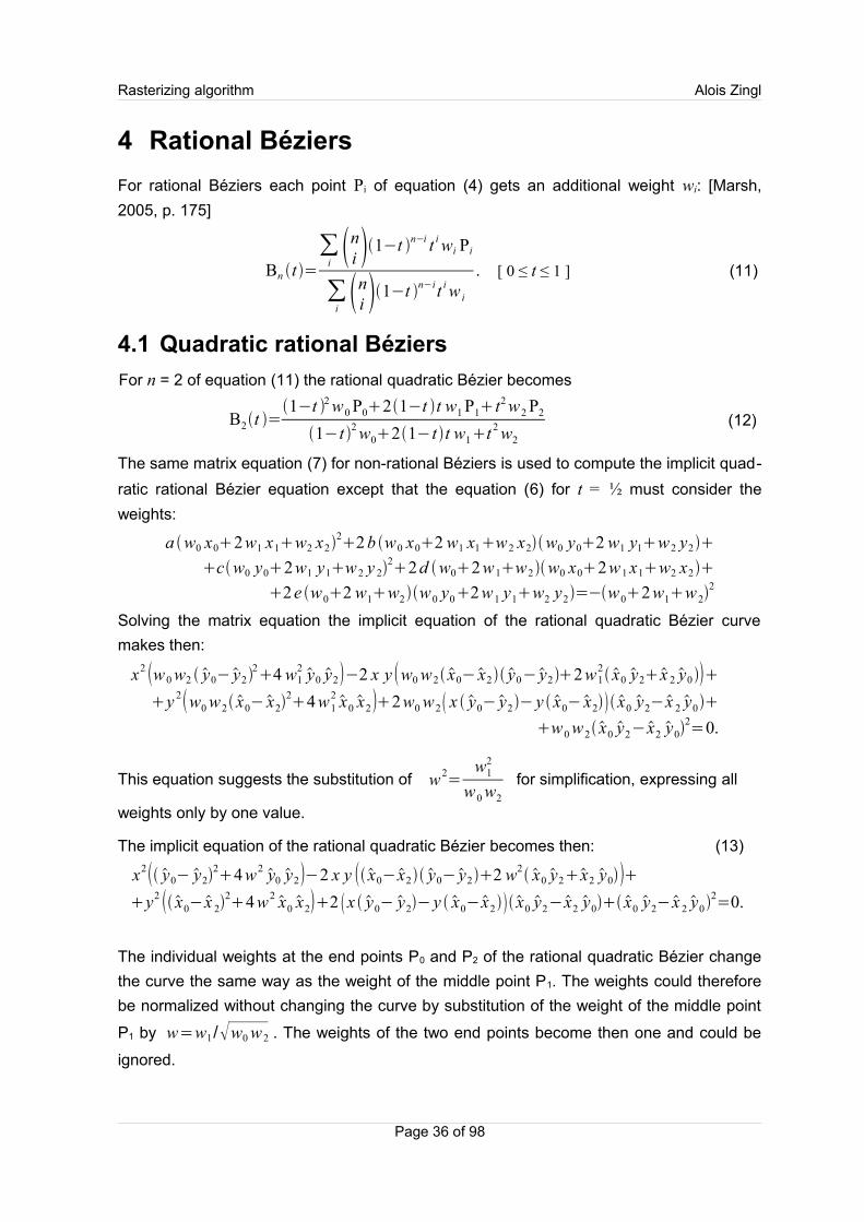
4.1 Quadratic rational Béziers
For n = 2 of equation (11) the rational quadratic Bézier becomes
B2t =1−t 2 w0 P021−t t w1 P1t2 w2 P2
1−t 2 w021−t t w1t 2 w2
(12)
The same matrix equation (7) for non-rational Béziers is used to compute the implicit quad-
ratic rational Bézier equation except that the equation (6) for t = ½ must consider the
weights:
a w0 x02w1 x1w2 x222b w0 x02 w1 x1w2 x2w0 y02 w1 y1w2 y2
cw0 y02w1 y1w 2 y 222d w02w1w2w0 x02w 1 x1w2 x2
2e w02 w1w2w0 y02w1 y1w2 y2=−w02w1w 22
Solving the matrix equation the implicit equation of the rational quadratic Bézier curve
makes then:
x2 w 0 w2 y0−y224 w1
2y0 y2−2 x y w0 w2 x0−x2 y0−y22w1
2 x0 y2x 2 y0
y 2w0 w2 x0−x224w1
2x0 x2 2w0 w2 x y0−y2− y x0−x2 x0 y2−x 2 y0
w0 w2 x0 y2−x2 y02=0.
This equation suggests the substitution of w2=
w12
w0 w2
for simplification, expressing all
weights only by one value.
The implicit equation of the rational quadratic Bézier becomes then: (13)
x2 y0− y224w2
y0 y2−2 x y x0−x2 y0−y22 w2 x0 y2x2 y0
y2 x0−x 224w2
x0 x22 x y0− y2− y x0−x2 x0 y2−x2 y0 x0 y2−x 2 y02=0.
The individual weights at the end points P0 and P2 of the rational quadratic Bézier change
the curve the same way as the weight of the middle point P1. The weights could therefore
be normalized without changing the curve by substitution of the weight of the middle point
P1 by w=w1/√w0 w2 . The weights of the two end points become then one and could be
ignored.
Page 36 of 98
Rasterizing algorithm Alois Zingl
For w =1 the curve is a parabola, for w < 1 the curve is an ellipse, for w = 0 the curve is a
straight line and for w >1 the curve is a hyperbola. The weights are normally assumed to be
all positive.
The quadratic Bézier curve must again be subdivided at horizontal and vertical turning
points. These four points are calculated by setting the first derivative of the parameter
equation (12) to zero:
t=2 w (P0−P1)−P0+P2±√ 4w2
(P0−P1)(P2−P1)+(P0−P2)2
2(w−1)(P0−P2). (14)
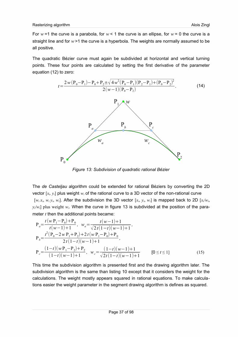
The de Casteljau algorithm could be extended for rational Béziers by converting the 2D
vector [xi, yi] plus weight wi of the rational curve to a 3D vector of the non-rational curve
[wi xi, wi yi, wi]. After the subdivision the 3D vector [xi, yi, wi] is mapped back to 2D [xi/wi,
yi/wi] plus weight wi. When the curve in figure 13 is subdivided at the position of the para-
meter t then the additional points became:
Pa=t (w P1−P0)+P0
t (w−1)+1, wa=
t(w−1)+1
√2 t(1−t)(w−1)+1,
Pb=t2(P0−2w P1+P2)+2 t (w P1−P0)+P0
2 t (1−t)(w−1)+1,
Pc=(1−t)(w P1−P2)+P2
(1−t )(w−1)+1, w c=
(1−t)(w−1)+1
√2t (1− t)(w−1)+1[0 ≤ t ≤ 1] (15)
This time the subdivision algorithm is presented first and the drawing algorithm later. The
subdivision algorithm is the same than listing 10 except that it considers the weight for the
calculations. The weight mostly appears squared in rational equations. To make calcula-
tions easier the weight parameter in the segment drawing algorithm is defines as squared.
Page 37 of 98
Figure 13: Subdivision of quadratic rational Bézier
P1
P2P
0
Pb
PcP
a
w
wa
wc
Rasterizing algorithm Alois Zingl
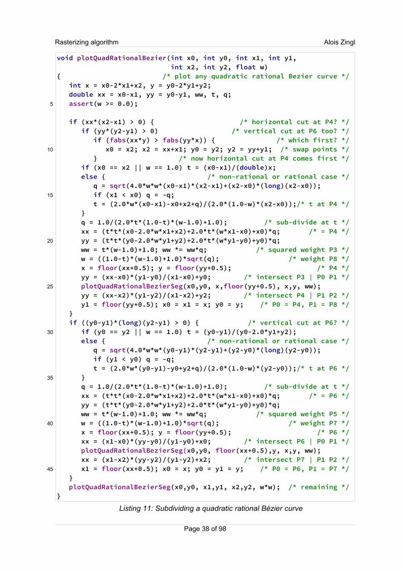
void plotQuadRationalBezier(int x0, int y0, int x1, int y1, int x2, int y2, float w){ /* plot any quadratic rational Bezier curve */ int x = x0-2*x1+x2, y = y0-2*y1+y2; double xx = x0-x1, yy = y0-y1, ww, t, q; assert(w >= 0.0); if (xx*(x2-x1) > 0) { /* horizontal cut at P4? */ if (yy*(y2-y1) > 0) /* vertical cut at P6 too? */ if (fabs(xx*y) > fabs(yy*x)) { /* which first? */ x0 = x2; x2 = xx+x1; y0 = y2; y2 = yy+y1; /* swap points */ } /* now horizontal cut at P4 comes first */ if (x0 == x2 || w == 1.0) t = (x0-x1)/(double)x; else { /* non-rational or rational case */ q = sqrt(4.0*w*w*(x0-x1)*(x2-x1)+(x2-x0)*(long)(x2-x0)); if (x1 < x0) q = -q; t = (2.0*w*(x0-x1)-x0+x2+q)/(2.0*(1.0-w)*(x2-x0));/* t at P4 */ } q = 1.0/(2.0*t*(1.0-t)*(w-1.0)+1.0); /* sub-divide at t */ xx = (t*t*(x0-2.0*w*x1+x2)+2.0*t*(w*x1-x0)+x0)*q; /* = P4 */ yy = (t*t*(y0-2.0*w*y1+y2)+2.0*t*(w*y1-y0)+y0)*q; ww = t*(w-1.0)+1.0; ww *= ww*q; /* squared weight P3 */ w = ((1.0-t)*(w-1.0)+1.0)*sqrt(q); /* weight P8 */ x = floor(xx+0.5); y = floor(yy+0.5); /* P4 */ yy = (xx-x0)*(y1-y0)/(x1-x0)+y0; /* intersect P3 | P0 P1 */ plotQuadRationalBezierSeg(x0,y0, x,floor(yy+0.5), x,y, ww); yy = (xx-x2)*(y1-y2)/(x1-x2)+y2; /* intersect P4 | P1 P2 */ y1 = floor(yy+0.5); x0 = x1 = x; y0 = y; /* P0 = P4, P1 = P8 */ } if ((y0-y1)*(long)(y2-y1) > 0) { /* vertical cut at P6? */ if (y0 == y2 || w == 1.0) t = (y0-y1)/(y0-2.0*y1+y2); else { /* non-rational or rational case */ q = sqrt(4.0*w*w*(y0-y1)*(y2-y1)+(y2-y0)*(long)(y2-y0)); if (y1 < y0) q = -q; t = (2.0*w*(y0-y1)-y0+y2+q)/(2.0*(1.0-w)*(y2-y0));/* t at P6 */ } q = 1.0/(2.0*t*(1.0-t)*(w-1.0)+1.0); /* sub-divide at t */ xx = (t*t*(x0-2.0*w*x1+x2)+2.0*t*(w*x1-x0)+x0)*q; /* = P6 */ yy = (t*t*(y0-2.0*w*y1+y2)+2.0*t*(w*y1-y0)+y0)*q; ww = t*(w-1.0)+1.0; ww *= ww*q; /* squared weight P5 */ w = ((1.0-t)*(w-1.0)+1.0)*sqrt(q); /* weight P7 */ x = floor(xx+0.5); y = floor(yy+0.5); /* P6 */ xx = (x1-x0)*(yy-y0)/(y1-y0)+x0; /* intersect P6 | P0 P1 */ plotQuadRationalBezierSeg(x0,y0, floor(xx+0.5),y, x,y, ww); xx = (x1-x2)*(yy-y2)/(y1-y2)+x2; /* intersect P7 | P1 P2 */ x1 = floor(xx+0.5); x0 = x; y0 = y1 = y; /* P0 = P6, P1 = P7 */ } plotQuadRationalBezierSeg(x0,y0, x1,y1, x2,y2, w*w); /* remaining */}
Listing 11: Subdividing a quadratic rational Bézier curve
Page 38 of 98
5
10
15
20
25
30
35
40
45
Rasterizing algorithm Alois Zingl
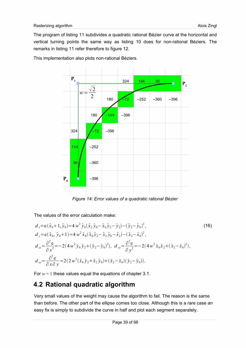
The program of listing 11 subdivides a quadratic rational Bézier curve at the horizontal and
vertical turning points the same way as listing 10 does for non-rational Béziers. The
remarks in listing 11 refer therefore to figure 12.
This implementation also plots non-rational Béziers.
The values of the error calculation make:
d x=e x01, y0=4 w2 y0 x2 y0−x0 y2− y2− y2−y02 , (16)
d y=e x0 , y01=4 w2 x0 x0 y2−x2 y0−x2− x2−x02 ,
d xx=∂
2 e∂ x2=−24w2
y0 y2 y2−y02 , d yy=
∂2e∂ y2=−24w2
x0 x 2 x2−x02 ,
d xy=∂
2 e∂ x∂ y
=22w2 x0 y2x2 y0 x2−x0 y2−y0.
For w = 1 these values equal the equations of chapter 3.1.
4.2 Rational quadratic algorithm
Very small values of the weight may cause the algorithm to fail. The reason is the same
than before. The other part of the ellipse comes too close. Although this is a rare case an
easy fix is simply to subdivide the curve in half and plot each segment separately.
Page 39 of 98
Figure 14: Error values of a quadratic rational Bézier
36144
–72
–144
–72
144
36 –360
–396
180
–396
–252
–396
180 –252
324
–360 –396
P0
P1
P2
324
w=√22
Rasterizing algorithm Alois Zingl
void plotQuadRationalBezierSeg(int x0, int y0, int x1, int y1, int x2, int y2, float w){ /* plot a limited rational Bezier segment, squared weight */ int sx = x2-x1, sy = y2-y1; /* relative values for checks */ double dx = x0-x2, dy = y0-y2, xx = x0-x1, yy = y0-y1; double xy = xx*sy+yy*sx, cur = xx*sy-yy*sx, err; /* curvature */
assert(xx*sx <= 0.0 && yy*sy <= 0.0); /* sign of gradient must not change */ if (cur != 0.0 && w > 0.0) { /* no straight line */ if (sx*(long)sx+sy*(long)sy > xx*xx+yy*yy) { /* begin with longer part */ x2 = x0; x0 -= dx; y2 = y0; y0 -= dy; cur = -cur; /* swap P0 P2 */ } xx = 2.0*(4.0*w*sx*xx+dx*dx); /* differences 2nd degree */ yy = 2.0*(4.0*w*sy*yy+dy*dy); sx = x0 < x2 ? 1 : -1; /* x step direction */ sy = y0 < y2 ? 1 : -1; /* y step direction */ xy = -2.0*sx*sy*(2.0*w*xy+dx*dy);
if (cur*sx*sy < 0.0) { /* negated curvature? */ xx = -xx; yy = -yy; xy = -xy; cur = -cur; } dx = 4.0*w*(x1-x0)*sy*cur+xx/2.0+xy; /* differences 1st degree */ dy = 4.0*w*(y0-y1)*sx*cur+yy/2.0+xy;
if (w < 0.5 && dy > dx) { /* flat ellipse, algorithm fails */ cur = (w+1.0)/2.0; w = sqrt(w); xy = 1.0/(w+1.0); sx = floor((x0+2.0*w*x1+x2)*xy/2.0+0.5); /* subdivide curve in half */ sy = floor((y0+2.0*w*y1+y2)*xy/2.0+0.5); dx = floor((w*x1+x0)*xy+0.5); dy = floor((y1*w+y0)*xy+0.5); plotQuadRationalBezierSeg(x0,y0, dx,dy, sx,sy, cur);/* plot separately */ dx = floor((w*x1+x2)*xy+0.5); dy = floor((y1*w+y2)*xy+0.5); plotQuadRationalBezierSeg(sx,sy, dx,dy, x2,y2, cur); return; } err = dx+dy-xy; /* error 1.step */ do { setPixel(x0,y0); /* plot curve */ if (x0 == x2 && y0 == y2) return; /* last pixel -> curve finished */ x1 = 2*err > dy; y1 = 2*(err+yy) < -dy;/* save value for test of x step */ if (2*err < dx || y1) { y0 += sy; dy += xy; err += dx += xx; }/* y step */ if (2*err > dx || x1) { x0 += sx; dx += xy; err += dy += yy; }/* x step */ } while (dy <= xy && dx >= xy); /* gradient negates -> algorithm fails */ } plotLine(x0,y0, x2,y2); /* plot remaining needle to end */}
Listing 12: Plot a limited rational Bezier segment
Page 40 of 98
5
10
15
20
25
30
35
40
45
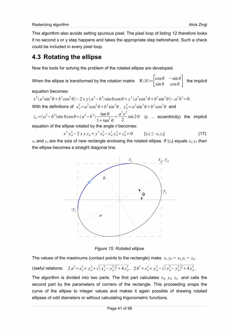
Rasterizing algorithm Alois Zingl
This algorithm also avoids setting spurious pixel. The pixel loop of listing 12 therefore looks
if no second x or y step happens and takes the appropriate step beforehand. Such a check
could be included in every pixel loop.
4.3 Rotating the ellipse
Now the tools for solving the problem of the rotated ellipse are developed.
When the ellipse is transformed by the rotation matrix R =[cos −sinsin cos ] the implicit
equation becomes:
x2a2sin2
b2 cos2−2 x y a2
−b2 sincos y2
a2cos2b2 sin2
−a2b2=0.
With the definitions of xd2=a2 cos2
b2sin2 , yd
2=a2sin 2
b2 cos2 and
zd=a2−b2sin cos=a2
−b2
tan1tan2
=
a2 e2
2sin 2 (e .. eccentricity) the implicit
equation of the ellipse rotated by the angle θ becomes:
x2 yd2−2 x y zd+ y2 xd
2−xd
2 yd2+ zd
2=0 [|zd| ≤ xd yd] (17)
xd and yd are the size of new rectangle enclosing the rotated ellipse. If |zd| equals xd yd then
the ellipse becomes a straight diagonal line.
Figure 15: Rotated ellipse
The values of the maximums (contact points to the rectangle) make xe yd = xd ye = zd.
Useful relations: 2 a2=xd
2+ yd
2+√( xd
2− yd
2)
2+4 zd
2 , 2b2=xd
2+ yd
2−√( xd
2− yd
2)
2+4 zd
2 .
The algorithm is divided into two parts. The first part calculates xd, yd, zd and calls the
second part by the parameters of corners of the rectangle. This proceeding snaps the
curve of the ellipse to integer values and makes it again possible of drawing rotated
ellipses of odd diameters or without calculating trigonometric functions.
Page 41 of 98
θ
a
b
xd , y
dx
e
ye
-ye
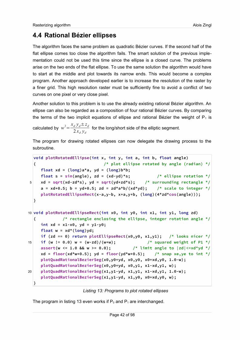
Rasterizing algorithm Alois Zingl
4.4 Rational Bézier ellipses
The algorithm faces the same problem as quadratic Bézier curves. If the second half of the
flat ellipse comes too close the algorithm fails. The smart solution of the previous imple-
mentation could not be used this time since the ellipse is a closed curve. The problems
arise on the two ends of the flat ellipse. To use the same solution the algorithm would have
to start at the middle and plot towards its narrow ends. This would become a complex
program. Another approach developed earlier is to increase the resolution of the raster by
a finer grid. This high resolution raster must be sufficiently fine to avoid a conflict of two
curves on one pixel or very close pixel.
Another solution to this problem is to use the already existing rational Bézier algorithm. An
ellipse can also be regarded as a composition of four rational Bézier curves. By comparing
the terms of the two implicit equations of ellipse and rational Bézier the weight of P1 is
calculated by w2=
xd yd± zd
2 xd yd
for the long/short side of the elliptic segment.
The program for drawing rotated ellipses can now delegate the drawing process to the
subroutine.
void plotRotatedEllipse(int x, int y, int a, int b, float angle){ /* plot ellipse rotated by angle (radian) */ float xd = (long)a*a, yd = (long)b*b; float s = sin(angle), zd = (xd-yd)*s; /* ellipse rotation */ xd = sqrt(xd-zd*s), yd = sqrt(yd+zd*s); /* surrounding rectangle */ a = xd+0.5; b = yd+0.5; zd = zd*a*b/(xd*yd); /* scale to integer */ plotRotatedEllipseRect(x-a,y-b, x+a,y+b, (long)(4*zd*cos(angle)));}
void plotRotatedEllipseRect(int x0, int y0, int x1, int y1, long zd){ /* rectangle enclosing the ellipse, integer rotation angle */ int xd = x1-x0, yd = y1-y0; float w = xd*(long)yd; if (zd == 0) return plotEllipseRect(x0,y0, x1,y1); /* looks nicer */ if (w != 0.0) w = (w-zd)/(w+w); /* squared weight of P1 */ assert(w <= 1.0 && w >= 0.0); /* limit angle to |zd|<=xd*yd */ xd = floor(xd*w+0.5); yd = floor(yd*w+0.5); /* snap xe,ye to int */ plotQuadRationalBezierSeg(x0,y0+yd, x0,y0, x0+xd,y0, 1.0-w); plotQuadRationalBezierSeg(x0,y0+yd, x0,y1, x1-xd,y1, w); plotQuadRationalBezierSeg(x1,y1-yd, x1,y1, x1-xd,y1, 1.0-w); plotQuadRationalBezierSeg(x1,y1-yd, x1,y0, x0+xd,y0, w);}
Listing 13: Programs to plot rotated ellipses
The program in listing 13 even works if P0 and P1 are interchanged.
Page 42 of 98
5
10
15
20

Rasterizing algorithm Alois Zingl
The only disadvantage of this solution is that the ellipse is not always exactly symmetric.
Sometimes the curve is just between two pixels and the drawing algorithm always rounds
to same direction (the lower pixel for example). In case of the ellipse this means that the
one side of the segment is rounded inwards and the other symmetric side outwards.
Page 43 of 98
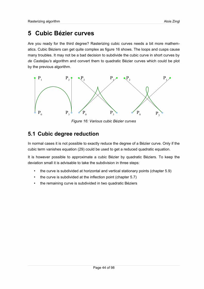
Rasterizing algorithm Alois Zingl
5 Cubic Bézier curves
Are you ready for the third degree? Rasterizing cubic curves needs a bit more mathem-
atics. Cubic Béziers can get quite complex as figure 16 shows. The loops and cusps cause
many troubles. It may not be a bad decision to subdivide the cubic curve in short curves by
de Casteljau's algorithm and convert them to quadratic Bézier curves which could be plot
by the previous algorithm.
5.1 Cubic degree reduction
In normal cases it is not possible to exactly reduce the degree of a Bézier curve. Only if the
cubic term vanishes equation (29) could be used to get a reduced quadratic equation.
It is however possible to approximate a cubic Bézier by quadratic Béziers. To keep the
deviation small it is advisable to take the subdivision in three steps:
• the curve is subdivided at horizontal and vertical stationary points (chapter 5.9)
• the curve is subdivided at the inflection point (chapter 5.7)
• the remaining curve is subdivided in two quadratic Béziers
Page 44 of 98
Figure 16: Various cubic Bézier curves
P0
P1
P2
P3
P0
P1
P2
P3
P0
P1
P2
P3
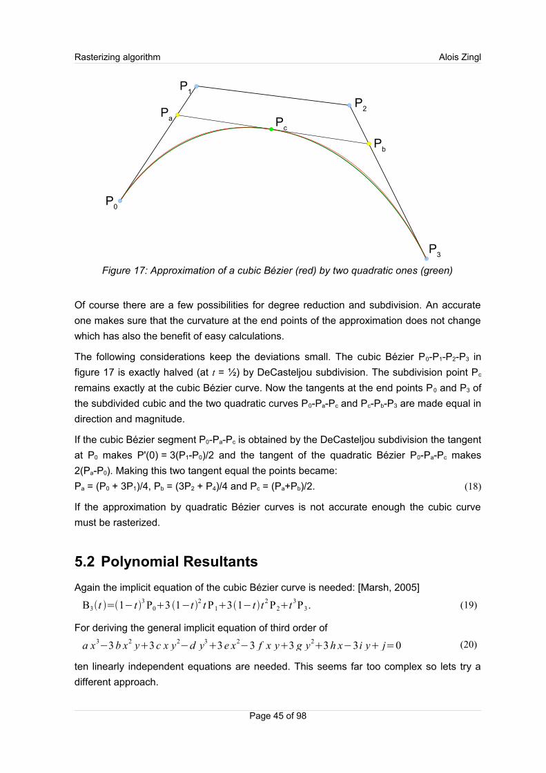
Rasterizing algorithm Alois Zingl
Figure 17: Approximation of a cubic Bézier (red) by two quadratic ones (green)
Of course there are a few possibilities for degree reduction and subdivision. An accurate
one makes sure that the curvature at the end points of the approximation does not change
which has also the benefit of easy calculations.
The following considerations keep the deviations small. The cubic Bézier P0-P1-P2-P3 in
figure 17 is exactly halved (at t = ½) by DeCasteljou subdivision. The subdivision point Pc
remains exactly at the cubic Bézier curve. Now the tangents at the end points P0 and P3 of
the subdivided cubic and the two quadratic curves P0-Pa-Pc and Pc-Pb-P3 are made equal in
direction and magnitude.
If the cubic Bézier segment P0-Pa-Pc is obtained by the DeCasteljou subdivision the tangent
at P0 makes P'(0) = 3(P1-P0)/2 and the tangent of the quadratic Bézier P0-Pa-Pc makes
2(Pa-P0). Making this two tangent equal the points became:
Pa = (P0 + 3P1)/4, Pb = (3P2 + P4)/4 and Pc = (Pa+Pb)/2. (18)
If the approximation by quadratic Bézier curves is not accurate enough the cubic curve
must be rasterized.
5.2 Polynomial Resultants
Again the implicit equation of the cubic Bézier curve is needed: [Marsh, 2005]
B3t =1− t 3 P03 1−t 2 t P131− t t 2 P2t 3P3 . (19)
For deriving the general implicit equation of third order of
a x3−3 b x2 y+3 c x y2
−d y3+3 e x2
−3 f x y+3 g y2+3 h x−3i y+ j=0 (20)
ten linearly independent equations are needed. This seems far too complex so lets try a
different approach.
Page 45 of 98
P0
P1
P2P
a Pc
P3
Pb
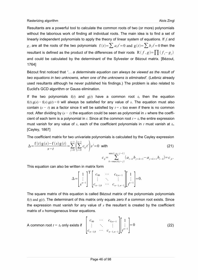
Rasterizing algorithm Alois Zingl
Resultants are a powerful tool to calculate the common roots of two (or more) polynomials
without the laborious work of finding all individual roots. The main idea is to find a set of
linearly independent polynomials to apply the theory of linear system of equations. If fi and
g j are all the roots of the two polynomials f t=∑ a i ti=0 and g t =∑ b i t
i=0 then the
resultant is defined as the product of the differences of their roots R f , g =∏ f i−g j
and could be calculated by the determinant of the Sylvester or Bézout matrix. [Bézout,
1764]
Bézout first noticed that '… a determinate equation can always be viewed as the result of
two equations in two unknowns, when one of the unknowns is eliminated'. (Leibniz already
used resultants although he never published his findings.) The problem is also related to
Euclid's GCD algorithm or Gauss elimination.
If the two polynomials f(t) and g(t) have a common root t0 then the equation
f(t) g(s) − f(s) g(t) = 0 will always be satisfied for any value of s. The equation must also
contain (s − t) as a factor since it will be satisfied by t = s too even if there is no common
root. After dividing by (s − t) the equation could be seen as polynomial in s where the coeffi-
cient of each term is a polynomial in t. Since at the common root t = t0 the entire expression
must vanish for any value of s, each of the coefficient polynomials in t must vanish at t0.
[Cayley, 1867]
The coefficient matrix for two univariate polynomials is calculated by the Cayley expression
=f t g s −f sg t
s−t=∑
j=0
n−1
∑i=0
n−1
cij tis j=0 with (21)
c ij= ∑k=max(0, i− j )
min (i ,n− j−1 )
(a i−k b j+k+1−a j+k+1 bi− k)=c ji .
This equation can also be written in matrix form
=[1⋮
sn−1]T
[c00 ⋯ c0,n−1
⋮ ⋱ ⋮cn−1,0 ⋯ cn−1, n−1
][1⋮
tn−1]=0.
The square matrix of this equation is called Bézout matrix of the polynomials polynomials
f(t) and g(t). The determinant of this matrix only equals zero if a common root exists. Since
the expression must vanish for any value of s the resultant is created by the coefficient
matrix of n homogeneous linear equations.
A common root t = t0 only exists if [c00 ⋯ c0,n−1
⋮ ⋱ ⋮cn−1,0 ⋯ cn−1,n−1
][ 1⋮
t n−1]=0 (22)
Page 46 of 98

Rasterizing algorithm Alois Zingl
It may be surprising to view this as linear equations but in this case the unknowns are
simply powers of t and the resultant will be identically equal to zero if and only if the coeffi-
cient matrix of n homogeneous linear equations of the power of t are all zero.
The simplest example is of degree one: f t=a1 ta0=0, g t=b1tb0=0.
(a1 t+a0)(b1 s+b0)−(a1 s+a0)(b1t+b0)
s−t=c00=a0b1−a1 b0=0.
The resultant of degree two is calculated by
f t =a2t 2a1ta0=0, gt =b2 t 2
b1tb0=0.
(a2 t 2+a1 t+a0)(b2 s2
+b1 s+b0)−(a2 s2+a1 s+a0)(b2 t 2
+b1 t+b0)
s−t=(c11 t+c01)s+(c01 t+c00)=0.
Bézout's matrix makes then [c00 c01
c10 c11][1t ]=[a0 b1−a1 b0 a0 b2−a2 b0
a0b2−a2 b0 a1 b2−a2 b1][1t ]=0.
The resultant of two cubic polynomials is calculated by
f t=a3t 3a2 t 2
a1 ta0=0, g t =b3t 3b2 t2
b1 tb0=0.
f (t)g (s)−f (s )g (t)s−t
=(c22 t 2+c12 t+c02)s
2+(c12 t 2
+c11 t+c10)s+(c02 t 2+c01 t+c00)=0.
The resultant of Bézout's matrix is
[a0b1−a1b0 a0 b2−a2b0 a0b3−a3 b0
a0 b2−a2 b0 a1b2−a2 b1+a0b3−a3 b0 a1b3−a3 b1
a0b3−a3 b0 a1 b3−a3b1 a2b3−a3 b2][ 1tt2]=0.
5.3 Implicit cubic Bézier equation
Now resultants can also be applied to convert the parametric equations of a curve to the
implicit form f(x,y)=0 for any value of t: R (f ,g)=∣c00 ⋯ c0, n−1
⋮ ⋱ ⋮cn−1,0 ⋯ cn−1,n−1
∣=0. (23)
The equation of the rational Bézier curve of degree n makes
Bn( t)=∑
i
w i(ni )(1−t )n−i ti P i
∑i
w i(ni )(1−t)n−i ti. (24)
The common root of the two parametric polynomials
f x t =∑i
wini 1−t n−i tix−x i=0 and f y t =∑
i
wini 1−t n−i t i y− y i=0
build the implicit equation of the Bézier curve f(x,y)=0 in x and y.
Page 47 of 98
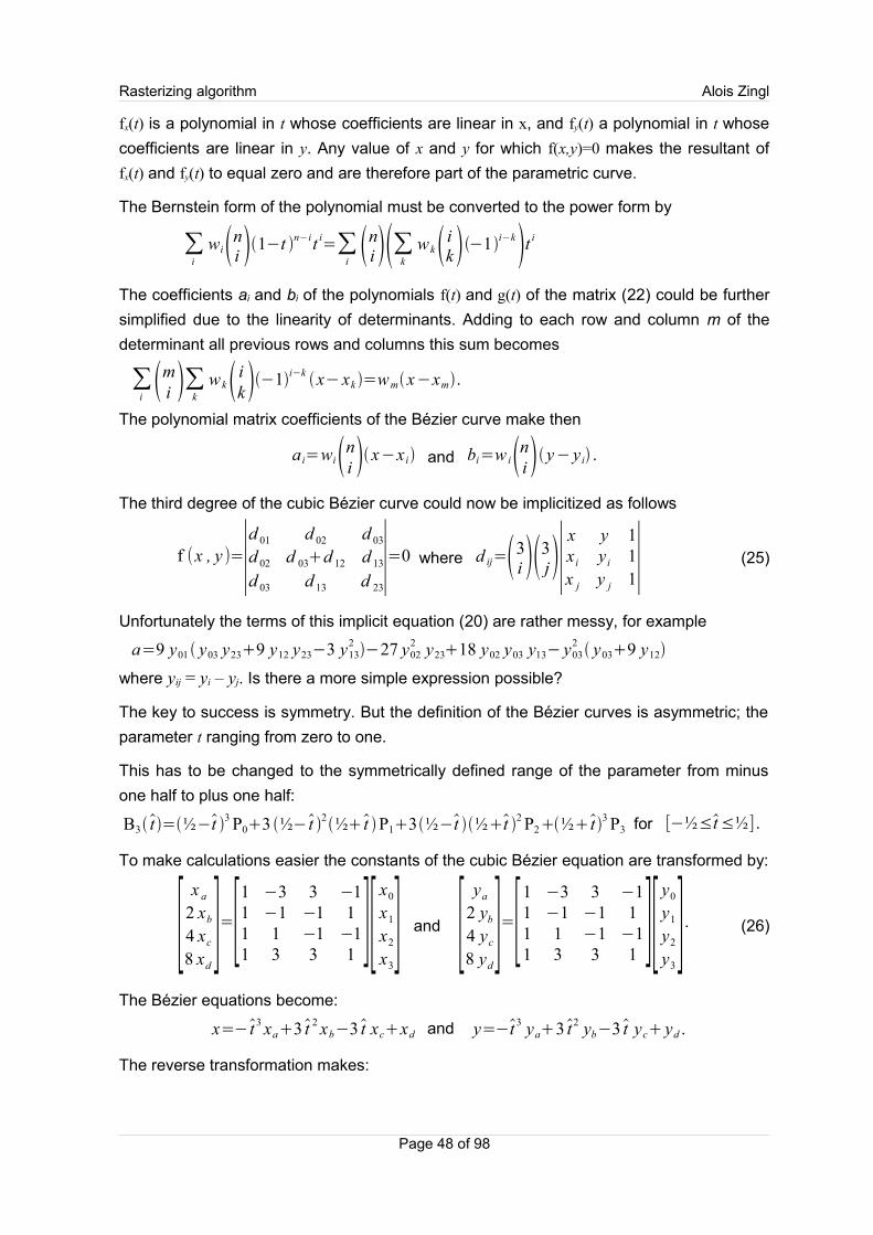
Rasterizing algorithm Alois Zingl
fx(t) is a polynomial in t whose coefficients are linear in x, and fy(t) a polynomial in t whose
coefficients are linear in y. Any value of x and y for which f(x,y)=0 makes the resultant of
fx(t) and fy(t) to equal zero and are therefore part of the parametric curve.
The Bernstein form of the polynomial must be converted to the power form by
∑i
wini 1−t n−it i=∑
ini ∑k w k ik−1i−kt i
The coefficients ai and bi of the polynomials f(t) and g(t) of the matrix (22) could be further
simplified due to the linearity of determinants. Adding to each row and column m of the
determinant all previous rows and columns this sum becomes
∑imi ∑k w k ik−1i−k
x− xk =wmx−xm.
The polynomial matrix coefficients of the Bézier curve make then
a i=wini x−x i and bi=w ini y− y i .
The third degree of the cubic Bézier curve could now be implicitized as follows
f (x , y )=∣d 01 d 02 d 03
d 02 d 03+d 12 d 13
d 03 d 13 d 23∣=0 where d ij=(3i )(3j)∣
x y 1x i y i 1x j y j 1∣ (25)
Unfortunately the terms of this implicit equation (20) are rather messy, for example
a=9 y01 y03 y239 y12 y23−3 y132−27 y02
2 y2318 y02 y03 y13− y032 y039 y12
where yij = yi – yj. Is there a more simple expression possible?
The key to success is symmetry. But the definition of the Bézier curves is asymmetric; the
parameter t ranging from zero to one.
This has to be changed to the symmetrically defined range of the parameter from minus
one half to plus one half:
B3 t =½−t 3 P03 ½−t 2½t P13½−t ½t 2 P2½t
3 P3 for [−½≤t≤½] .
To make calculations easier the constants of the cubic Bézier equation are transformed by:
[x a
2 xb
4 xc
8 xd]=[
1 −3 3 −11 −1 −1 11 1 −1 −11 3 3 1
][x0
x1
x2
x3] and [
ya
2 yb
4 yc
8 yd]=[
1 −3 3 −11 −1 −1 11 1 −1 −11 3 3 1
][y0
y1
y2
y3]. (26)
The Bézier equations become:
x=−t 3 xa3 t 2 xb−3 t xcxd and y=−t 3 ya3 t2 yb−3 t yc yd .
The reverse transformation makes:
Page 48 of 98
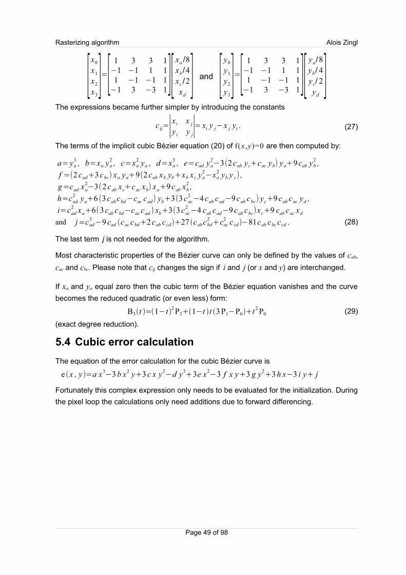
Rasterizing algorithm Alois Zingl
[x0
x1
x2
x3]=[
1 3 3 1−1 −1 1 11 −1 −1 1−1 3 −3 1
][xa /8xb/4xc /2xd] and [
y0
y1
y2
y3]=[
1 3 3 1−1 −1 1 11 −1 −1 1−1 3 −3 1
][ya/8yb/ 4yc/ 2yd]
The expressions became further simpler by introducing the constants
c ij=∣x i x j
y i y j∣= xi y j−x j yi . (27)
The terms of the implicit cubic Bézier equation (20) of f(x ,y)=0 are then computed by:
a= ya3 , b=xa ya
2 , c=xa2 ya , d=xa
3 , e=cad ya2−3(2cab yc+cac yb) ya+9cab yb
2 ,
f =(2cad+3cbc) xa ya+9(2cab xb yb+xb xc ya2−xa
2 yb y c) ,
g=cad xa2−3(2cab xc+cac xb) xa+9cab xb
2 ,
h=cad2 ya+6 (3cabcbd−cac cad) yb+3(3cac
2−4cab cad−9cab cbc) yc+9cab cac yd ,
i=cad2 xa+6(3cab cbd−cac cad ) xb+3(3cac
2−4 cab cad−9cab cbc)xc+9 cab cac xd
and j=cad3−9 cad cac cbd2cab ccd 27 cabcbd
2cac
2 ccd −81cab cbc ccd . (28)
The last term j is not needed for the algorithm.
Most characteristic properties of the Bézier curve can only be defined by the values of cab,
cac and cbc. Please note that cij changes the sign if i and j (or x and y) are interchanged.
If xa and ya equal zero then the cubic term of the Bézier equation vanishes and the curve
becomes the reduced quadratic (or even less) form:
B3t =1−t 2 P31−t t 3 P1−P0t 2 P0 (29)
(exact degree reduction).
5.4 Cubic error calculation
The equation of the error calculation for the cubic Bézier curve is
e x , y =a x3−3b x2 y3c x y2
−d y33e x2
−3 f x y3 g y23h x−3 i y j
Fortunately this complex expression only needs to be evaluated for the initialization. During
the pixel loop the calculations only need additions due to forward differencing.
Page 49 of 98
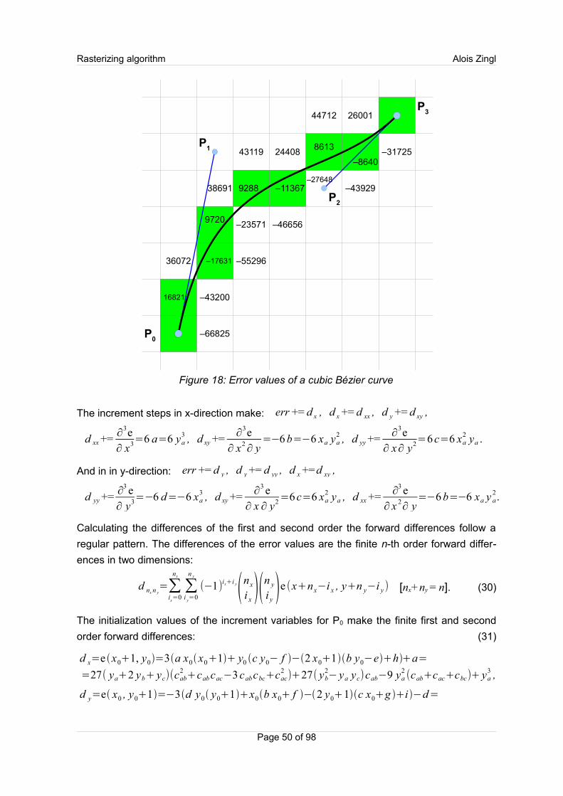
Rasterizing algorithm Alois Zingl
The increment steps in x-direction make: err += d x , d x += d xx , d y += d xy ,
d xx +=∂
3e∂ x3=6 a=6 ya
3 , d xy +=∂
3e∂ x2∂ y=−6b=−6 xa ya
2 , d yy +=∂
3e∂ x∂ y2=6c=6 xa
2 ya .
And in in y-direction: err += d y , d y += d yy , d x +=d xy ,
d yy +=∂
3 e∂ y3=−6 d=−6 xa
3 , d xy +=∂
3 e∂ x ∂ y2=6c=6 xa
2 ya , d xx +=∂
3 e∂ x 2∂ y=−6b=−6 xa y a
2.
Calculating the differences of the first and second order the forward differences follow a
regular pattern. The differences of the error values are the finite n-th order forward differ-
ences in two dimensions:
d nx n y=∑
ix=0
nx
∑i y=0
n y
(−1)ix+i y(nx
i x )(n y
i y )e (x+nx−i x , y+n y−i y ) [nx+ ny = n]. (30)
The initialization values of the increment variables for P0 make the finite first and second
order forward differences: (31)
d x=e x01, y0=3a x0x01 y0 c y0− f −2 x01b y0−eha=
=27( ya+2 yb+ yc)(cab2+cab cac−3 cabcbc+cac
2)+27( yb
2− ya yc)cab−9 ya
2(cab+cac+cbc)+ ya
3 ,
d y=e x0 , y01=−3d y0 y01x0b x0 f −2 y01c x0g i −d=
Page 50 of 98
Figure 18: Error values of a cubic Bézier curve
–8640
8613
–113679288
9720
–17631
16821 –43200
36072
–23571
–66825
–55296
–46656
43119 24408
–43929
–31725
P0
P1
P2
P32600144712
38691–27648
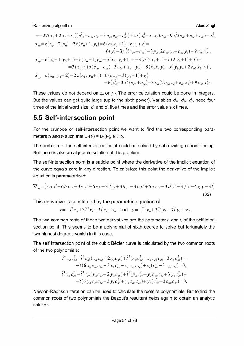
Rasterizing algorithm Alois Zingl
=−27xa2 xbxc cab2cab cac−3cab cbccac
227 xb
2−xa xc cab−9 xa
2cabcaccbc− xa
3 ,
d xx=e x02, y0−2e x01, y0=6 a x01−b y0e=
=6 ya3−3 y a
2cabcac −3 ya 2 cab yccac yb9cab yb
2 ,
d xy=e x01, y01−e x01, y0−e x0 , y01=−3b 2 x01−c 2 y01 f =
=3xa ya 6cabcac−3cbc xa− ya−9xb xc ya2−xa
2 yb yc2cab xb yb ,
d yy=e x0 , y02−2 e x0 , y01=6 c x0−d y01g =
=6xa3−3 xa
2cabcac−3 xa 2cab xccac xb9cab xb
2 .
These values do not depend on xd or yd. The error calculation could be done in integers.
But the values can get quite large (up to the sixth power). Variables dxx, dxy, dyy need four
times of the initial word size, dx and dy five times and the error value six times.
5.5 Self-intersection point
For the crunode or self-intersection point we want to find the two corresponding para-
meters t1 and t2 such that B3(t1) = B3(t2), t1 ≠ t2.
The problem of the self-intersection point could be solved by sub-dividing or root finding.
But there is also an algebraic solution of this problem.
The self-intersection point is a saddle point where the derivative of the implicit equation of
the curve equals zero in any direction. To calculate this point the derivative of the implicit
equation is parameterized:
∇ xy=⟨3a x2−6b x y3c y2
6e x−3 f y3h , −3b x26c x y−3 d y2
−3 f x6 g y−3i ⟩(32)
This derivative is substituted by the parametric equation of
x=−t 3 xa3 t 2 xb−3 t xcxd and y=−t 3 ya3 t2 yb−3 t yc yd .
The two common roots of these two derivatives are the parameter t1 and t2 of the self inter-
section point. This seems to be a polynomial of sixth degree to solve but fortunately the
two highest degrees vanish in this case.
The self intersection point of the cubic Bézier curve is calculated by the two common roots
of the two polynomials:
t 4 xa cab2−t 3 cabxa cac2 xbcabt
2xa cac
2−xa cab cbc3 xc cab
2
t 6 xb cab cbc−3 xb cac2xa cac cbcxc cac
2−3 cabcbc=0,
t 4 ya cab2−t 3 cab ya cac2 yb cabt
2 ya cac
2− ya cab cbc3 yc cab
2
t 6 yb cabcbc−3 yb cac2 ya cac cbc yc cac
2−3cab cbc=0.
Newton-Raphson iteration can be used to calculate the roots of polynomials. But to find the
common roots of two polynomials the Bezout's resultant helps again to obtain an analytic
solution.
Page 51 of 98
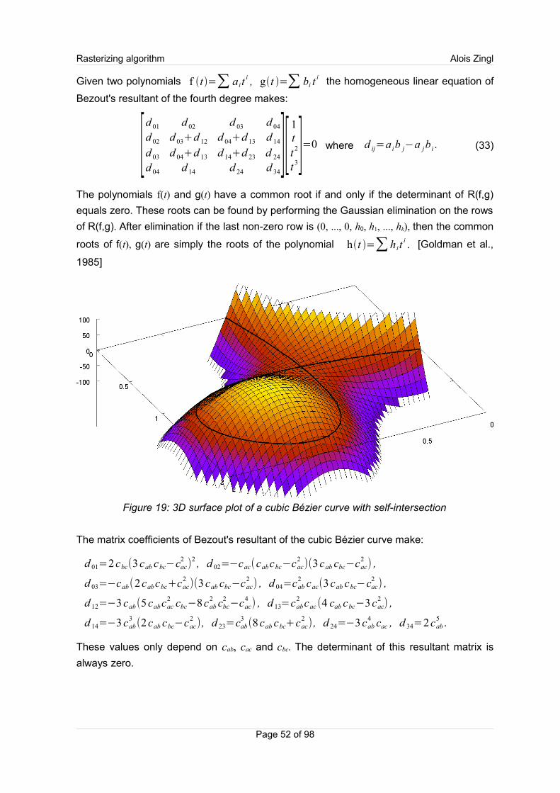
Rasterizing algorithm Alois Zingl
Given two polynomials f t=∑ a i ti , gt =∑ bi t
i the homogeneous linear equation of
Bezout's resultant of the fourth degree makes:
[d 01 d 02 d 03 d 04
d 02 d 03+d 12 d 04+d 13 d 14
d 03 d 04+d 13 d 14+d 23 d 24
d 04 d 14 d 24 d 34][
1tt 2
t 3]=0 where d ij=a ib j−a jb i . (33)
The polynomials f(t) and g(t) have a common root if and only if the determinant of R(f,g)
equals zero. These roots can be found by performing the Gaussian elimination on the rows
of R(f,g). After elimination if the last non-zero row is (0, ..., 0, h0, h1, ..., hk), then the common
roots of f(t), g(t) are simply the roots of the polynomial ht =∑ h i ti . [Goldman et al.,
1985]
The matrix coefficients of Bezout's resultant of the cubic Bézier curve make:
d 01=2cbc(3cab cbc−cac2)
2 , d 02=−cac(cabcbc−cac2)(3cab cbc−cac
2) ,
d 03=−cab(2cabcbc+cac2)(3cab cbc−cac
2) , d 04=cab
2 cac(3cab cbc−cac2) ,
d 12=−3 cab(5cabcac2 cbc−8cab
2 cbc2−cac
4) , d 13=cab
2 cac (4 cab cbc−3cac2) ,
d 14=−3 cab3(2cab cbc−cac
2) , d 23=cab
3(8cab cbc+cac
2) , d 24=−3cab
4 cac , d 34=2cab5 .
These values only depend on cab, cac and cbc. The determinant of this resultant matrix is
always zero.
Page 52 of 98
Figure 19: 3D surface plot of a cubic Bézier curve with self-intersection
Rasterizing algorithm Alois Zingl
Eliminating one row and column of the matrix gets the quadratic equation to calculate the
roots of the self-intersection point. Taking row 2 and 3 the parameter of the self-intersec-
tion point makes: t 1,2=cac±12 cab cbc−3 cac
2
2 cab
. (34)
Please note that t 1 and t 2 also do not depend on xd, yd, which are like the center of the
Bézier curve.
For 4 cabcbccac2 the cubic implicit equation has a complex self-intersection point
(acnode). If 4 cabcbc=cac2 the curve has a cusp. If ∣t 1,2∣½ then the cubic Bézier
segment has a self-intersection point (crunode). Otherwise only the implicit equation
outside the parameter interval has a self-intersection.
5.6 Gradient at P0
The gradient of the curve at P0 is either positive or negative in plot direction. Since the
algorithm depends on a continuously positive (or negative) slope the values have to be
negated in case of a negative gradient to be able to use the same algorithm. How to calcu-
late the gradient at P0?
The gradient is the cross product of the surface normal and the curve tangent vector.
The normal to the surface of the equation e(x,y) = z in figure (20) makes
n=[−∂e (x , y )∂ x
,−∂e (x , y )∂ y
,1].With the definition of the grade g=
274((cab+cac)
2−cab(cac+3cbc)) the derivatives of the
equation make∂e x0, y0
∂ x=g y0− y1 and
∂e x0, y0
∂ y=−g x0−x1. The gradient at
Page 53 of 98
Figure 20: Curve gradient
x
yz
gz
Rasterizing algorithm Alois Zingl
P0 makes then
∇ e x0 , y0=n×[ x1−x0, y1− y0 ,0]=[ y0− y1 , x1− x0 , g x0− x12 y0− y1
2].
The z component (gz in figure 20) of the gradient (proportional to g) is only negative if P0 is
part of the self intersection loop. If the grade g equals zero the point P0 itself is the crunode
(or cusp).
This information can be used to take special care since drawing the self-intersection loop
always includes the danger that another part of the curve comes too close for the algorithm
to work correctly.
5.7 Inflection point
The position of the inflection points becomes important if the cubic Bézier is approximated
by sets of connected quadratic Bézier segments. A cubic Bézier curve changes its bending
direction at the inflection point.
The inflection point is the point where the curvature of a curve equals zero. The curvature
of a curve is calculated by κ=1r=
d φd s=∣B(t)×B( t )∣
∣B(t )∣3=
f x (t) ¨f y (t)− f y( t) f x (t)
√( f x2(t )+ ˙f y
2(t))
3. (35)
In case of the cubic Bézier curve the inflection point could be determined by the quadratic
equation of t 2cab−t caccbc=0. (36)
5.8 Cubic troubles
Again the algorithm runs into troubles for certain Bézier curves. Figure 21 shows a curve
with ambitious error values at P0. The situation becomes clear if the entire curve is plotted.
The point at P0 is near a self intersection point.
The algorithm has a real dilemma with flat self-intersection loops. It cannot plot from the
intersection side since the error values change sign there. If the algorithm wants to plot
from the flat tip side there is the danger that the other part of the curve is too close and the
error values are too confusing. The algorithm fails if the curve contains a flat self-intersec-
tion loop.
Figure 21 shows a curve where the loop is very flat. In that case both ends could be acute
angles and lead into narrow or same pixel. The algorithm can not plot a curve if both ends
start with such confusing error values. Two possibilities could solve the problem. The first
would be the same used for quadratic rational Béziers. The curve is additionally subdivided
at the broadest position of the loop and the plot starts there. The curves get a bit edgy
sometimes by this solution. The other one is to use a higher resolution raster for the plot.
The resolution is selected by the length of the legs. This method slightly decreases the plot
speed but leads to smoother curves.
Page 54 of 98

Rasterizing algorithm Alois Zingl
5.9 Cubic algorithm
The basic algorithm needs a continuously rising or falling curve. It is not even simple to
include a check of the parameters to ensure this condition. The first is that the lines P1-P0
and P3-P2 are both either rising or falling. But the slope of P2-P1 could be negated to the
others and the curve could still be plot. So the second condition must be that either the line
P3-P0 has the same slope than P2-P1 or the first derivative of the parametric equation has
real roots.
The assert statement must also consider certain rounding errors. If the parameter is of
single floating point type with 23 bit mantissa and the parameter of the coordinates don't
exceed 16 bit then epsilon must be greater than 216-23.
For simple (and faster) code the calculation of dx and dxx is one y-step ahead. The calcula-
tion of dy and dyy is one x-step ahead. The calculation of the error value is one x- and one y-
step ahead.
The cubic Bézier curve could have a cusp or self-intersection loop. Even if the loop is not
directly visible with the specific parameter the entire curve could have a loop and the
visible segment be a part of it. This cusp or loop causes many troubles. The algorithm can
not plot through the self-intersection. Therefore the plot starts from both ends. If the error
values get confused because the gradient changes its sign then the other end is tried.
Consequently the function is able to handle Bézier curves with self-intersection points.
Another problem arises if this loop is very flat like in figure 21. Then one end of the curve is
prossibly blocked by the self-intersection point and on the other end has too confusing
Page 55 of 98
Figure 21: Cubic Bézier with confusing error values
46
–71188
–37
–27
–4681
432
–1
19
2592
8
1215 54
487
P0
P1
P2
P3
791
1765
1934
–26
–98
188
784
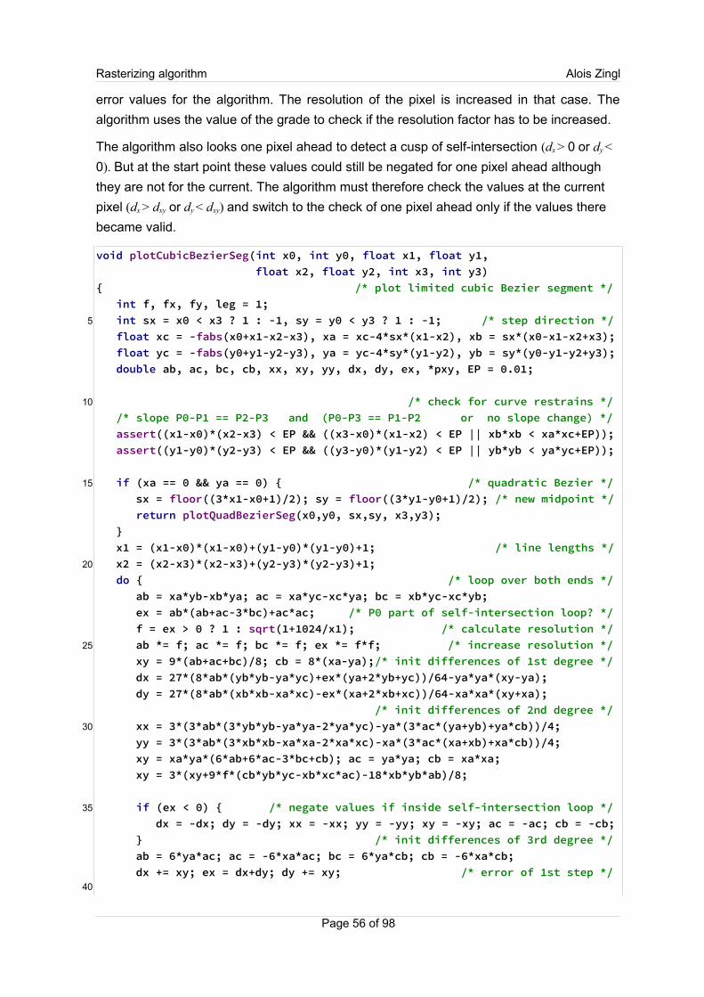
Rasterizing algorithm Alois Zingl
error values for the algorithm. The resolution of the pixel is increased in that case. The
algorithm uses the value of the grade to check if the resolution factor has to be increased.
The algorithm also looks one pixel ahead to detect a cusp of self-intersection (dx > 0 or dy <
0). But at the start point these values could still be negated for one pixel ahead although
they are not for the current. The algorithm must therefore check the values at the current
pixel (dx > dxy or dy < dxy) and switch to the check of one pixel ahead only if the values there
became valid.
void plotCubicBezierSeg(int x0, int y0, float x1, float y1, float x2, float y2, int x3, int y3) { /* plot limited cubic Bezier segment */ int f, fx, fy, leg = 1; int sx = x0 < x3 ? 1 : -1, sy = y0 < y3 ? 1 : -1; /* step direction */ float xc = -fabs(x0+x1-x2-x3), xa = xc-4*sx*(x1-x2), xb = sx*(x0-x1-x2+x3); float yc = -fabs(y0+y1-y2-y3), ya = yc-4*sy*(y1-y2), yb = sy*(y0-y1-y2+y3); double ab, ac, bc, cb, xx, xy, yy, dx, dy, ex, *pxy, EP = 0.01; /* check for curve restrains */ /* slope P0-P1 == P2-P3 and (P0-P3 == P1-P2 or no slope change) */ assert((x1-x0)*(x2-x3) < EP && ((x3-x0)*(x1-x2) < EP || xb*xb < xa*xc+EP)); assert((y1-y0)*(y2-y3) < EP && ((y3-y0)*(y1-y2) < EP || yb*yb < ya*yc+EP));
if (xa == 0 && ya == 0) { /* quadratic Bezier */ sx = floor((3*x1-x0+1)/2); sy = floor((3*y1-y0+1)/2); /* new midpoint */ return plotQuadBezierSeg(x0,y0, sx,sy, x3,y3); } x1 = (x1-x0)*(x1-x0)+(y1-y0)*(y1-y0)+1; /* line lengths */ x2 = (x2-x3)*(x2-x3)+(y2-y3)*(y2-y3)+1; do { /* loop over both ends */ ab = xa*yb-xb*ya; ac = xa*yc-xc*ya; bc = xb*yc-xc*yb; ex = ab*(ab+ac-3*bc)+ac*ac; /* P0 part of self-intersection loop? */ f = ex > 0 ? 1 : sqrt(1+1024/x1); /* calculate resolution */ ab *= f; ac *= f; bc *= f; ex *= f*f; /* increase resolution */ xy = 9*(ab+ac+bc)/8; cb = 8*(xa-ya);/* init differences of 1st degree */ dx = 27*(8*ab*(yb*yb-ya*yc)+ex*(ya+2*yb+yc))/64-ya*ya*(xy-ya); dy = 27*(8*ab*(xb*xb-xa*xc)-ex*(xa+2*xb+xc))/64-xa*xa*(xy+xa); /* init differences of 2nd degree */ xx = 3*(3*ab*(3*yb*yb-ya*ya-2*ya*yc)-ya*(3*ac*(ya+yb)+ya*cb))/4; yy = 3*(3*ab*(3*xb*xb-xa*xa-2*xa*xc)-xa*(3*ac*(xa+xb)+xa*cb))/4; xy = xa*ya*(6*ab+6*ac-3*bc+cb); ac = ya*ya; cb = xa*xa; xy = 3*(xy+9*f*(cb*yb*yc-xb*xc*ac)-18*xb*yb*ab)/8;
if (ex < 0) { /* negate values if inside self-intersection loop */ dx = -dx; dy = -dy; xx = -xx; yy = -yy; xy = -xy; ac = -ac; cb = -cb; } /* init differences of 3rd degree */ ab = 6*ya*ac; ac = -6*xa*ac; bc = 6*ya*cb; cb = -6*xa*cb; dx += xy; ex = dx+dy; dy += xy; /* error of 1st step */
Page 56 of 98
5
10
15
20
25
30
35
40

Rasterizing algorithm Alois Zingl
for (pxy = &xy, fx = fy = f; x0 != x3 && y0 != y3; ) { setPixel(x0,y0); /* plot curve */ do { /* move sub-steps of one pixel */ if (dx > *pxy || dy < *pxy) goto exit; /* confusing values */ y1 = 2*ex-dy; /* save value for test of y step */ if (2*ex >= dx) { /* x sub-step */ fx--; ex += dx += xx; dy += xy += ac; yy += bc; xx += ab; } if (y1 <= 0) { /* y sub-step */ fy--; ex += dy += yy; dx += xy += bc; xx += ac; yy += cb; } } while (fx > 0 && fy > 0); /* pixel complete? */ if (2*fx <= f) { x0 += sx; fx += f; } /* x step */ if (2*fy <= f) { y0 += sy; fy += f; } /* y step */ if (pxy == &xy && dx < 0 && dy > 0) pxy = &EP;/* pixel ahead valid */ } exit: xx = x0; x0 = x3; x3 = xx; sx = -sx; xb = -xb; /* swap legs */ yy = y0; y0 = y3; y3 = yy; sy = -sy; yb = -yb; x1 = x2; } while (leg--); /* try other end */ plotLine(x0,y0, x3,y3); /* remaining part in case of cusp or crunode */}
Listing 14: Plotting a cubic Bézier segment
The algorithm tries to plot from either end of the curve and stops if the error values get
confused. This happens in case of a self-intersection and especially of a cusp. The curve is
then finished by a line.
It would be possible to test the break condition of the pixel loop just for the end point. But if
the end point is missed due to a slight rounding error the algorithm wouldn't stop. The
implementation in listing 14 ensures that the curve is not plot beyond the end point.
A few further optimizations are possible like writing a separate loop for curves without loop
(self intersection). This would reduce the overhead in the pixel loop for most the drawn
Bézier curves. A reference could be used instead of the pointer variable if applicable.
The algorithm could be simplified if no cubic Bézier curves with a loop or cusp have to be
rasterized. The variation for increased resolution could be omitted in that case.
Page 57 of 98
45
50
55
60
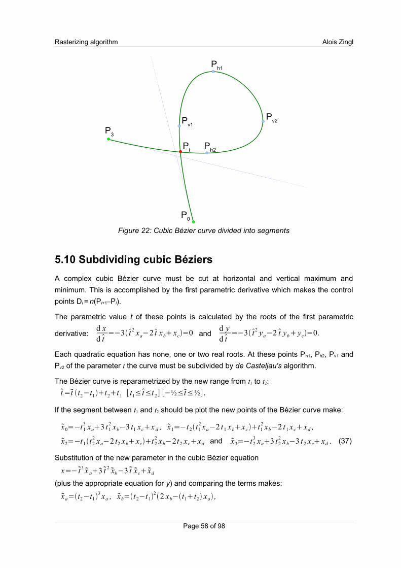
Rasterizing algorithm Alois Zingl
5.10 Subdividing cubic Béziers
A complex cubic Bézier curve must be cut at horizontal and vertical maximum and
minimum. This is accomplished by the first parametric derivative which makes the control
points Di = n(Pi+1–Pi).
The parametric value t of these points is calculated by the roots of the first parametric
derivative: d xd t=−3 t 2 xa−2 t xb xc=0 and
d yd t=−3 t2 ya−2 t yb yc=0.
Each quadratic equation has none, one or two real roots. At these points Ph1, Ph2, Pv1 and
Pv2 of the parameter t the curve must be subdivided by de Casteljau's algorithm.
The Bézier curve is reparametrized by the new range from t1 to t2:
t=t t2−t1t2t1 [ t1≤t≤t 2] [−½≤t≤½] .
If the segment between t1 and t2 should be plot the new points of the Bézier curve make:
x0=−t13 xa3 t 1
2 xb−3 t1 xcx d , x1=−t 2t12 xa−2 t 1 xbxc t1
2 xb−2 t 1 xc xd ,
x2=−t1t 22 xa−2 t2 xb xct 2
2 xb−2t 2 xcxd and x3=−t 23 xa3 t 2
2 xb−3 t 2 xc xd . (37)
Substitution of the new parameter in the cubic Bézier equation
x=−t 3x a3 t 2
xb−3 t xcxd
(plus the appropriate equation for y) and comparing the terms makes:
xa=t2−t13 xa , xb=t 2−t 1
22 xb−t1 t2 xa ,
Page 58 of 98
Figure 22: Cubic Bézier curve divided into segments
P0
Pi
Ph2
Ph1
P3
Pv2P
v1

Rasterizing algorithm Alois Zingl
xc=t 2−t 1t1t 22 xa−4t 1t 2xb4 xc and
xd=−t 1t 23 xa6t 1t 2
2 xb−12 t1t2 xc8x d . (38)
5.11 Drawing any cubic Bézier curve
The Bézier curve is subdivided at horizontal and vertical gradient changes. These points
are then sorted to get consecutive curve segments. Since only four points at most have to
be sorted the simplest sorting algorithm is efficiently enough. The curve is not subdivided
at self-intersection point since the sub-segment plot function is able to handle this case.
Another problem would arise when the intermediate points P1 or P2 are rounded to integers
due to the subdivision. It could happen that the carefully avoided situation of gradient
change suddenly reappears again due to the rounding. To avoid a significant change only
the boundary of the subdivided curve is therefore scaled to integers. For this reason the
intermediate points of the sub-segment plot function must be of floating point type.
It is essential that the computation of the parameter t is of double accuracy especially the
square root function. Insufficient accuracy may change the parameter of the subdivided
curve slightly so that it does not match the necessary restrains anymore and the assert
statement in the sub-segment function would fail.
Page 59 of 98
Figure 23: Horizontal and vertical roots of a cubic Bézier
Ph1
Pv2
Pv1
Ph2
D0
D1
D2
P1-P
0
P2-P
1
P3-P
2
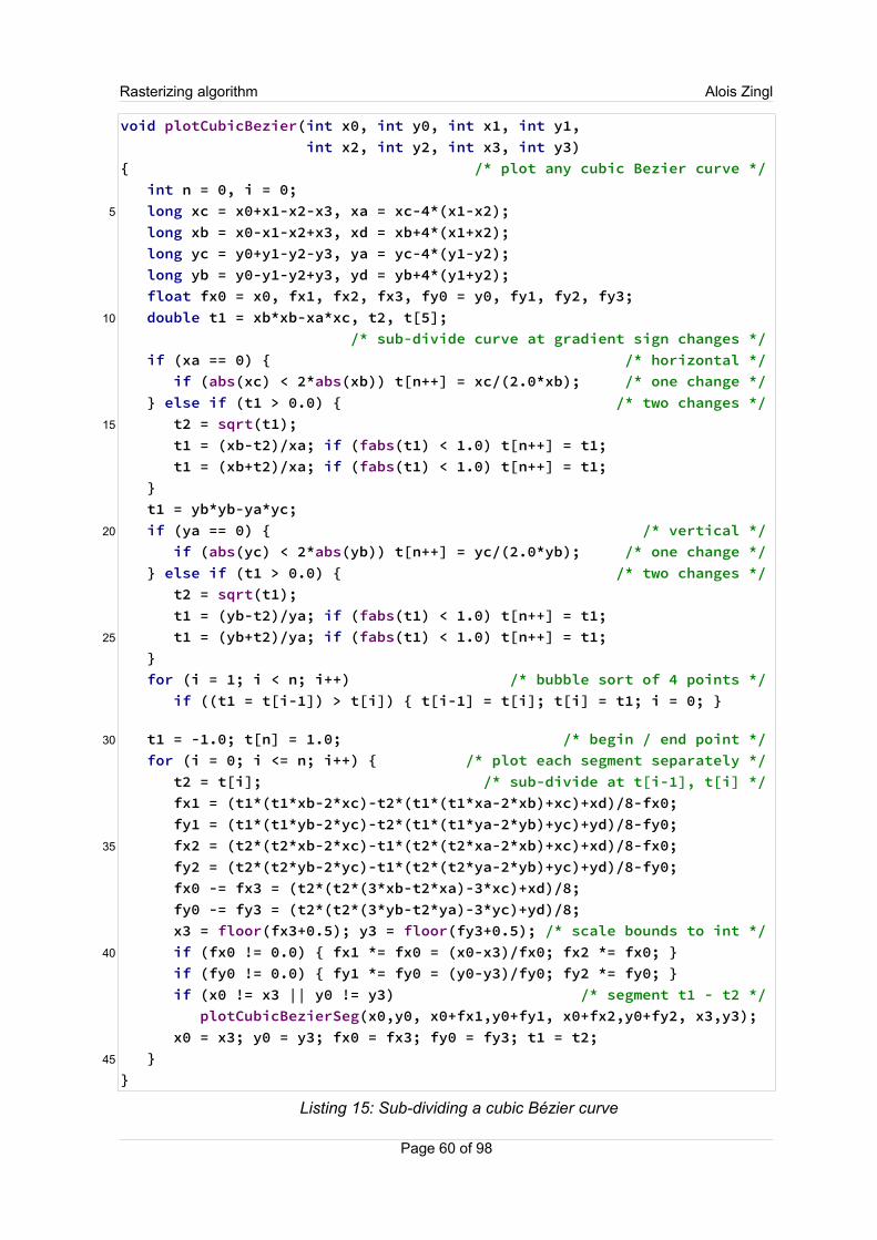
Rasterizing algorithm Alois Zingl
void plotCubicBezier(int x0, int y0, int x1, int y1, int x2, int y2, int x3, int y3){ /* plot any cubic Bezier curve */ int n = 0, i = 0; long xc = x0+x1-x2-x3, xa = xc-4*(x1-x2); long xb = x0-x1-x2+x3, xd = xb+4*(x1+x2); long yc = y0+y1-y2-y3, ya = yc-4*(y1-y2); long yb = y0-y1-y2+y3, yd = yb+4*(y1+y2); float fx0 = x0, fx1, fx2, fx3, fy0 = y0, fy1, fy2, fy3; double t1 = xb*xb-xa*xc, t2, t[5]; /* sub-divide curve at gradient sign changes */ if (xa == 0) { /* horizontal */ if (abs(xc) < 2*abs(xb)) t[n++] = xc/(2.0*xb); /* one change */ } else if (t1 > 0.0) { /* two changes */ t2 = sqrt(t1); t1 = (xb-t2)/xa; if (fabs(t1) < 1.0) t[n++] = t1; t1 = (xb+t2)/xa; if (fabs(t1) < 1.0) t[n++] = t1; } t1 = yb*yb-ya*yc; if (ya == 0) { /* vertical */ if (abs(yc) < 2*abs(yb)) t[n++] = yc/(2.0*yb); /* one change */ } else if (t1 > 0.0) { /* two changes */ t2 = sqrt(t1); t1 = (yb-t2)/ya; if (fabs(t1) < 1.0) t[n++] = t1; t1 = (yb+t2)/ya; if (fabs(t1) < 1.0) t[n++] = t1; } for (i = 1; i < n; i++) /* bubble sort of 4 points */ if ((t1 = t[i-1]) > t[i]) { t[i-1] = t[i]; t[i] = t1; i = 0; }
t1 = -1.0; t[n] = 1.0; /* begin / end point */ for (i = 0; i <= n; i++) { /* plot each segment separately */ t2 = t[i]; /* sub-divide at t[i-1], t[i] */ fx1 = (t1*(t1*xb-2*xc)-t2*(t1*(t1*xa-2*xb)+xc)+xd)/8-fx0; fy1 = (t1*(t1*yb-2*yc)-t2*(t1*(t1*ya-2*yb)+yc)+yd)/8-fy0; fx2 = (t2*(t2*xb-2*xc)-t1*(t2*(t2*xa-2*xb)+xc)+xd)/8-fx0; fy2 = (t2*(t2*yb-2*yc)-t1*(t2*(t2*ya-2*yb)+yc)+yd)/8-fy0; fx0 -= fx3 = (t2*(t2*(3*xb-t2*xa)-3*xc)+xd)/8; fy0 -= fy3 = (t2*(t2*(3*yb-t2*ya)-3*yc)+yd)/8; x3 = floor(fx3+0.5); y3 = floor(fy3+0.5); /* scale bounds to int */ if (fx0 != 0.0) { fx1 *= fx0 = (x0-x3)/fx0; fx2 *= fx0; } if (fy0 != 0.0) { fy1 *= fy0 = (y0-y3)/fy0; fy2 *= fy0; } if (x0 != x3 || y0 != y3) /* segment t1 - t2 */ plotCubicBezierSeg(x0,y0, x0+fx1,y0+fy1, x0+fx2,y0+fy2, x3,y3); x0 = x3; y0 = y3; fx0 = fx3; fy0 = fy3; t1 = t2; }}
Listing 15: Sub-dividing a cubic Bézier curve
Page 60 of 98
5
10
15
20
25
30
35
40
45

Rasterizing algorithm Alois Zingl
The middle control points P1 and P2 could be changed to the thru points P1 , P2 by
P1=−5P018 P1−9 P22P3
6and P2=
2P0−9 P118 P2−5 P3
6. (39)
Page 61 of 98
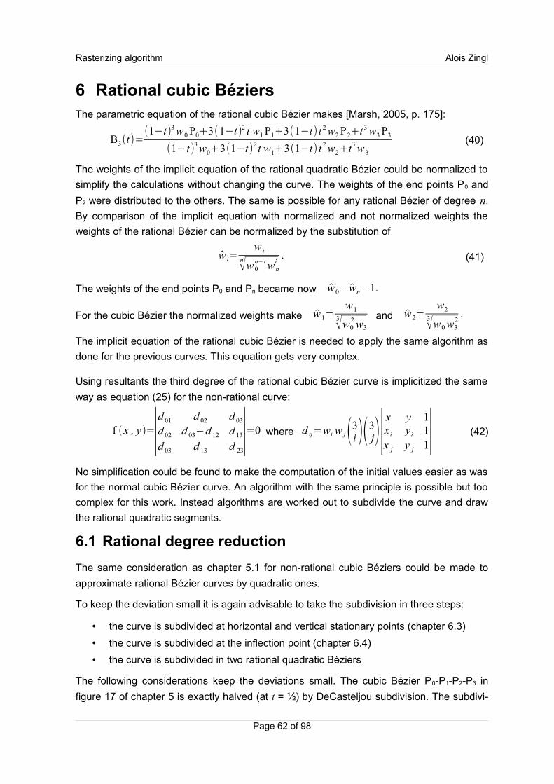
Rasterizing algorithm Alois Zingl
6 Rational cubic BéziersThe parametric equation of the rational cubic Bézier makes [Marsh, 2005, p. 175]:
B3(t)=(1−t)3 w0 P0+3(1−t )2 t w1 P1+3(1−t) t 2 w2 P2+t 3 w3 P3
(1− t)3 w0+3(1−t)2t w1+3(1−t) t 2 w2+t3 w3
(40)
The weights of the implicit equation of the rational quadratic Bézier could be normalized to
simplify the calculations without changing the curve. The weights of the end points P0 and
P2 were distributed to the others. The same is possible for any rational Bézier of degree n.
By comparison of the implicit equation with normalized and not normalized weights the
weights of the rational Bézier can be normalized by the substitution of
w i=w i
nw 0n−i wn
i. (41)
The weights of the end points P0 and Pn became now w0= wn=1.
For the cubic Bézier the normalized weights make w1=w1
3w02 w3
and w2=w2
3w0 w32.
The implicit equation of the rational cubic Bézier is needed to apply the same algorithm as
done for the previous curves. This equation gets very complex.
Using resultants the third degree of the rational cubic Bézier curve is implicitized the same
way as equation (25) for the non-rational curve:
f x , y =∣d 01 d 02 d 03
d 02 d 03d 12 d 13
d 03 d 13 d 23∣=0 where d ij=wi w j(3i )(3j)∣
x y 1x i y i 1x j y j 1∣ (42)
No simplification could be found to make the computation of the initial values easier as was
for the normal cubic Bézier curve. An algorithm with the same principle is possible but too
complex for this work. Instead algorithms are worked out to subdivide the curve and draw
the rational quadratic segments.
6.1 Rational degree reduction
The same consideration as chapter 5.1 for non-rational cubic Béziers could be made to
approximate rational Bézier curves by quadratic ones.
To keep the deviation small it is again advisable to take the subdivision in three steps:
• the curve is subdivided at horizontal and vertical stationary points (chapter 6.3)
• the curve is subdivided at the inflection point (chapter 6.4)
• the curve is subdivided in two rational quadratic Béziers
The following considerations keep the deviations small. The cubic Bézier P0-P1-P2-P3 in
figure 17 of chapter 5 is exactly halved (at t = ½) by DeCasteljou subdivision. The subdivi-
Page 62 of 98
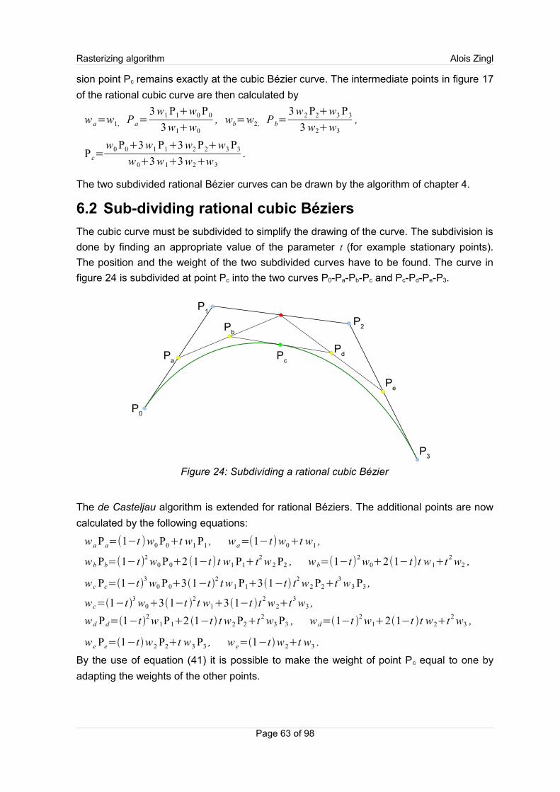
Rasterizing algorithm Alois Zingl
sion point Pc remains exactly at the cubic Bézier curve. The intermediate points in figure 17
of the rational cubic curve are then calculated by
wa=w1, Pa=3 w1 P1+w0 P0
3 w1+w0
, wb=w2, Pb=3 w2 P2+w3 P3
3 w2+w3
,
Pc=w0 P0+3 w1 P1+3 w2 P2+w3 P3
w0+3 w1+3 w2+w3
.
The two subdivided rational Bézier curves can be drawn by the algorithm of chapter 4.
6.2 Sub-dividing rational cubic Béziers
The cubic curve must be subdivided to simplify the drawing of the curve. The subdivision is
done by finding an appropriate value of the parameter t (for example stationary points).
The position and the weight of the two subdivided curves have to be found. The curve in
figure 24 is subdivided at point Pc into the two curves P0-Pa-Pb-Pc and Pc-Pd-Pe-P3.
The de Casteljau algorithm is extended for rational Béziers. The additional points are now
calculated by the following equations:
wa Pa=(1−t )w0 P0+t w1 P1 , wa=(1−t)w0+t w1 ,
wb Pb=(1− t)2 w0 P0+2 (1−t) t w1 P1+ t2 w2 P2 , wb=(1−t)2 w0+2(1−t)t w1+t 2 w2 ,
w c Pc=1−t 3 w0 P031−t 2 t w1 P131−t t2 w2 P2t3 w3 P3 ,
w c=1−t 3 w031−t 2t w131−t t 2 w2t 3 w3 ,
wd Pd=1−t 2 w1P12 1−t t w2 P2t 2 w3 P3 , wd=1−t 2 w121−t t w2t 2 w3 ,
w e Pe=1−t w2 P2t w3 P3 , w e=1−t w2t w3 .
By the use of equation (41) it is possible to make the weight of point Pc equal to one by
adapting the weights of the other points.
Page 63 of 98
Figure 24: Subdividing a rational cubic Bézier
P0
P1
P2
Pa
Pb
P3
Pe
Pc
Pd

Rasterizing algorithm Alois Zingl
6.3 Root findingThe rational cubic Bézier must be subdivided at the stationary points. These points are the
maximums and minimums of the curve in x- and y-direction. These points can be
calculated by setting the first derivation of the parametric equation (40) to zero. This
equation becomes a bit simpler by introducing the substitution of P ij=wi−w jPi P j.
P01−2P02P033P12−2P13P23 t4−2 2P01−3 P02P033P12−3 P13t
3
6P01−6P02P033P12t2−22 P01−P02tP01=0.
This equation is a polynomial of the fourth degree. The analytical calculation of the roots of
the fourth degree is possible but difficult. The following solution tries to find an algorithm
as simple as possible.
Only the real roots are of interest for this application. If the highest coefficient of the
following polynomial equations is zero the equation could be reduced by one degree. The
coefficient is therefore by assumed to be unequal to zero.
The accuracy of the calculation needs special attention. The numbers can get quite large
due to the powers. Rounding errors occur if such large numbers are added or subtracted
due to the limited accuracy of the calculation.
The implementations are as simple as possible and use a minimum of transcendental
functions.
6.3.1 Quadratic equation
For the quadratic polynomial equation a2 x2+a1 x+a0=0 the substitution of
p=−a1
2a2
, q=a0
a2
makes the calculation easier.
The number of real roots depends on the discriminant shown in the following table:
Discriminant Number of real roots Root value(s)
p 2 < q 0 -
p 2 = q 1 x = p
p 2 > q 2x1= p+√ p2
−qx2=q/ x1
The calculation of x2 by the division is more stable than the negative root.
6.3.2 Cubic equation
For the cubic polynomial equation a3 x3+a2 x2
+a1 x+a0=0 the substitution of
p=−a2
3a3
, q= p2−
a1
3a3
, r=3q− p2
2p
a0
2a3
makes the calculation again easier.
Page 64 of 98
Rasterizing algorithm Alois Zingl
These definitions also show the degree relations between the coefficients which is relevant
to avoid an underflow of floating point numbers.
The substitution of x = z + p gets the depressed cubic z3−3q z+2 r=0. By Vieta's
substitution of z = y + q / y this equation could be turned into a quadratic equation in y3:
y6+2 r y3+q3=0. Back substitution gets the roots of the cubic equation.
The number of real roots depends on the discriminant shown in the following table:
Discriminant Number of real roots Root value(s)
r = 0 q = 0∧ 1 x = p
r 2 > q 3 1 y=3 r r2
−q3
x= p yq / y
r 2 = q 3 2x1= p+r / qx2= p−2 r /q
r 2 < q 3 3
y=q cos13 arccosr
q3 x1= p−2 y
x2,3=p y±3 q− y2
The last case uses the substitution of z=2√q cosθ for the depressed cubic to avoid the calculations of complex numbers. Dividing the equation by 2√q3 gets the cubic equation
of 4 cos3θ−3cos θ+
r
√q3=0. Comparison with the equation of cos3=4cos3
−3cos
gets the relation of cos3=−r
q3. The roots are then calculated by the entries of the
table above.
6.3.3 Quartic equation
For the quartic polynomial equation a4 x4a3 x3
a2 x2a1 xa0=0 the substitution of
p=−a3
4a4
, q=3 p2−
a2
2a4
, r=q− p2 p−
a1
4a4
, s= p2−2q p4 r p−
a0
a4
makes
the calculation once again easier.
The substitution x = z + p gets rid of the cubic term: z 4−2q z2
−4 r z−s=0
If r equals zero this is a quadratic equation in z2. The original quartic is then solved by:
x= p±1q±2q2s [r = 0]
If r does not equal zero the quartic equation can be turned to the solution of a resolvent
cubic equation by several methods [Shmakov, 2011]. The algorithm of Euler solves the
quartic equation by the resolvent cubic equation of:
4 y3−4q y2
q2s y−r2
=0
This cubic equation can be solved by the method of the previous chapter. It always has a
positive root.
Page 65 of 98
Rasterizing algorithm Alois Zingl
If y is a positive root of the cubic equation then the roots of the original quartic make
x= p±1q− y±2 r / y±2 y [r ≠ 0]
The subscript of the plus/minus sign indicate the same sign of the four different solutions of
the quartic equation. Only real roots are of interest for this application.
6.4 Rational inflection point
The calculation of the inflection point of the rational cubic Bézier is a bit more complicated
than of the non-rational Bézier. Equation (35) is again used to get the curvature of the
curve. The following substitution makes the computation easier:
c ijk=w i w j wk∣x i y i 1x j y j 1xk yk 1∣.
The inflection points of the rational cubic Bézier curve could now be determined by the
cubic equation of
t 3c012−c013c023−c123−t 2
3 c012−2 c013c023t 3 c012−c013−c012=0. (43)
The roots of this equation could be solved using the method of the previous chapter.
Page 66 of 98
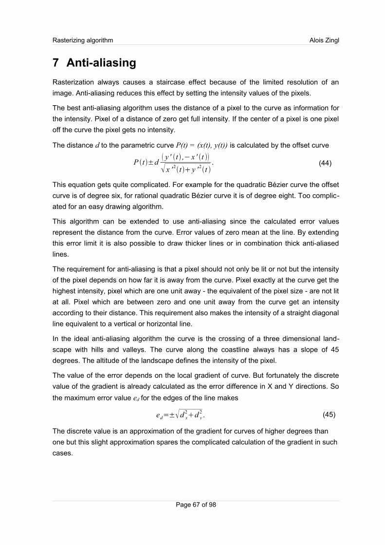
Rasterizing algorithm Alois Zingl
7 Anti-aliasing
Rasterization always causes a staircase effect because of the limited resolution of an
image. Anti-aliasing reduces this effect by setting the intensity values of the pixels.
The best anti-aliasing algorithm uses the distance of a pixel to the curve as information for
the intensity. Pixel of a distance of zero get full intensity. If the center of a pixel is one pixel
off the curve the pixel gets no intensity.
The distance d to the parametric curve P(t) = (x(t), y(t)) is calculated by the offset curve
P t ±d y ' t ,− x ' t
x ' 2t y ' 2
t . (44)
This equation gets quite complicated. For example for the quadratic Bézier curve the offset
curve is of degree six, for rational quadratic Bézier curve it is of degree eight. Too complic-
ated for an easy drawing algorithm.
This algorithm can be extended to use anti-aliasing since the calculated error values
represent the distance from the curve. Error values of zero mean at the line. By extending
this error limit it is also possible to draw thicker lines or in combination thick anti-aliased
lines.
The requirement for anti-aliasing is that a pixel should not only be lit or not but the intensity
of the pixel depends on how far it is away from the curve. Pixel exactly at the curve get the
highest intensity, pixel which are one unit away - the equivalent of the pixel size - are not lit
at all. Pixel which are between zero and one unit away from the curve get an intensity
according to their distance. This requirement also makes the intensity of a straight diagonal
line equivalent to a vertical or horizontal line.
In the ideal anti-aliasing algorithm the curve is the crossing of a three dimensional land-
scape with hills and valleys. The curve along the coastline always has a slope of 45
degrees. The altitude of the landscape defines the intensity of the pixel.
The value of the error depends on the local gradient of curve. But fortunately the discrete
value of the gradient is already calculated as the error difference in X and Y directions. So
the maximum error value ed for the edges of the line makes
ed=±√d x2+d y
2 . (45)
The discrete value is an approximation of the gradient for curves of higher degrees than
one but this slight approximation spares the complicated calculation of the gradient in such
cases.
Page 67 of 98
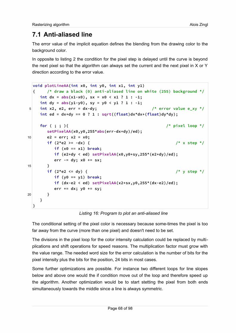
Rasterizing algorithm Alois Zingl
7.1 Anti-aliased lineThe error value of the implicit equation defines the blending from the drawing color to the
background color.
In opposite to listing 2 the condition for the pixel step is delayed until the curve is beyond
the next pixel so that the algorithm can always set the current and the next pixel in X or Y
direction according to the error value.
void plotLineAA(int x0, int y0, int x1, int y1){ /* draw a black (0) anti-aliased line on white (255) background */ int dx = abs(x1-x0), sx = x0 < x1 ? 1 : -1; int dy = abs(y1-y0), sy = y0 < y1 ? 1 : -1; int x2, e2, err = dx-dy; /* error value e_xy */ int ed = dx+dy == 0 ? 1 : sqrt((float)dx*dx+(float)dy*dy);
for ( ; ; ){ /* pixel loop */ setPixelAA(x0,y0,255*abs(err-dx+dy)/ed); e2 = err; x2 = x0; if (2*e2 >= -dx) { /* x step */ if (x0 == x1) break; if (e2+dy < ed) setPixelAA(x0,y0+sy,255*(e2+dy)/ed); err -= dy; x0 += sx; } if (2*e2 <= dy) { /* y step */ if (y0 == y1) break; if (dx-e2 < ed) setPixelAA(x2+sx,y0,255*(dx-e2)/ed); err += dx; y0 += sy; } }}
Listing 16: Program to plot an anti-aliased line
The conditional setting of the pixel color is necessary because some-times the pixel is too
far away from the curve (more than one pixel) and doesn't need to be set.
The divisions in the pixel loop for the color intensity calculation could be replaced by multi-
plications and shift operations for speed reasons. The multiplication factor must grow with
the value range. The needed word size for the error calculation is the number of bits for the
pixel intensity plus the bits for the position, 24 bits in most cases.
Some further optimizations are possible. For instance two different loops for line slopes
below and above one would the if condition move out of the loop and therefore speed up
the algorithm. Another optimization would be to start stetting the pixel from both ends
simultaneously towards the middle since a line is always symmetric.
Page 68 of 98
5
10
15
20
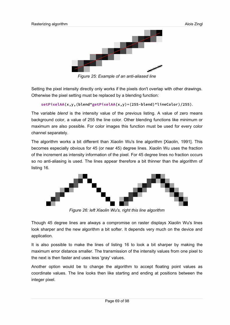
Rasterizing algorithm Alois Zingl
Figure 25: Example of an anti-aliased line
Setting the pixel intensity directly only works if the pixels don't overlap with other drawings.
Otherwise the pixel setting must be replaced by a blending function:
setPixelAA(x,y,(blend*getPixelAA(x,y)+(255-blend)*lineColor)/255).
The variable blend is the intensity value of the previous listing. A value of zero means
background color, a value of 255 the line color. Other blending functions like minimum or
maximum are also possible. For color images this function must be used for every color
channel separately.
The algorithm works a bit different than Xiaolin Wu's line algorithm [Xiaolin, 1991]. This
becomes especially obvious for 45 (or near 45) degree lines. Xiaolin Wu uses the fraction
of the increment as intensity information of the pixel. For 45 degree lines no fraction occurs
so no anti-aliasing is used. The lines appear therefore a bit thinner than the algorithm of
listing 16.
Figure 26: left Xiaolin Wu's, right this line algorithm
Though 45 degree lines are always a compromise on raster displays Xiaolin Wu's lines
look sharper and the new algorithm a bit softer. It depends very much on the device and
application.
It is also possible to make the lines of listing 16 to look a bit sharper by making the
maximum error distance smaller. The transmission of the intensity values from one pixel to
the next is then faster and uses less 'gray' values.
Another option would be to change the algorithm to accept floating point values as
coordinate values. The line looks then like starting and ending at positions between the
integer pixel.
Page 69 of 98
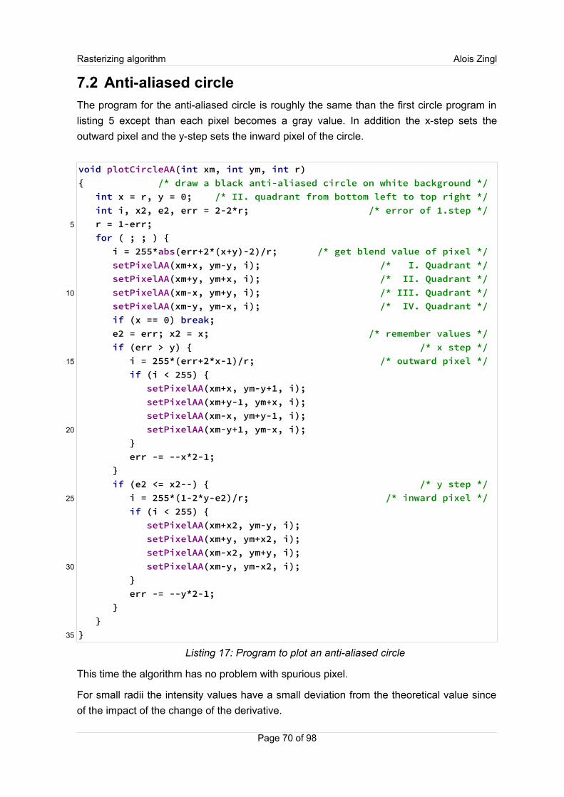
Rasterizing algorithm Alois Zingl
7.2 Anti-aliased circleThe program for the anti-aliased circle is roughly the same than the first circle program in
listing 5 except than each pixel becomes a gray value. In addition the x-step sets the
outward pixel and the y-step sets the inward pixel of the circle.
void plotCircleAA(int xm, int ym, int r){ /* draw a black anti-aliased circle on white background */ int x = r, y = 0; /* II. quadrant from bottom left to top right */ int i, x2, e2, err = 2-2*r; /* error of 1.step */ r = 1-err; for ( ; ; ) { i = 255*abs(err+2*(x+y)-2)/r; /* get blend value of pixel */ setPixelAA(xm+x, ym-y, i); /* I. Quadrant */ setPixelAA(xm+y, ym+x, i); /* II. Quadrant */ setPixelAA(xm-x, ym+y, i); /* III. Quadrant */ setPixelAA(xm-y, ym-x, i); /* IV. Quadrant */ if (x == 0) break; e2 = err; x2 = x; /* remember values */ if (err > y) { /* x step */ i = 255*(err+2*x-1)/r; /* outward pixel */ if (i < 255) { setPixelAA(xm+x, ym-y+1, i); setPixelAA(xm+y-1, ym+x, i); setPixelAA(xm-x, ym+y-1, i); setPixelAA(xm-y+1, ym-x, i); } err -= --x*2-1; } if (e2 <= x2--) { /* y step */ i = 255*(1-2*y-e2)/r; /* inward pixel */ if (i < 255) { setPixelAA(xm+x2, ym-y, i); setPixelAA(xm+y, ym+x2, i); setPixelAA(xm-x2, ym+y, i); setPixelAA(xm-y, ym-x2, i); } err -= --y*2-1; } } }
Listing 17: Program to plot an anti-aliased circle
This time the algorithm has no problem with spurious pixel.
For small radii the intensity values have a small deviation from the theoretical value since
of the impact of the change of the derivative.
Page 70 of 98
5
10
15
20
25
30
35
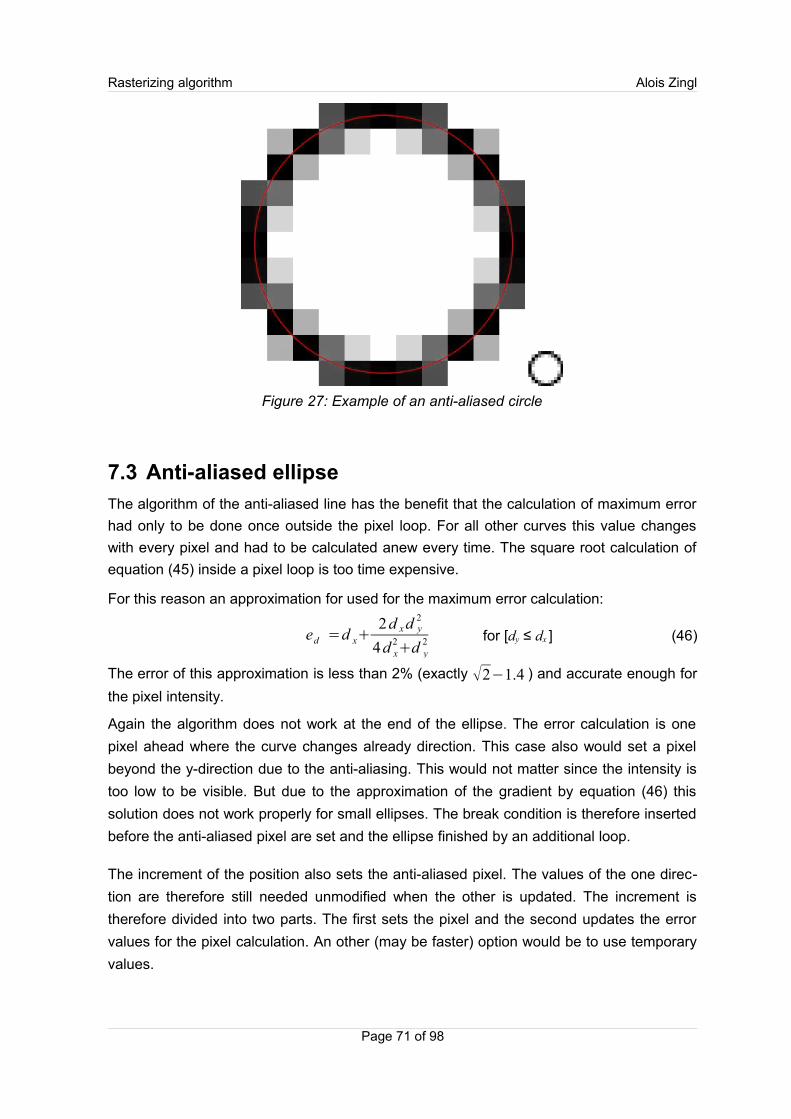
Rasterizing algorithm Alois Zingl
Figure 27: Example of an anti-aliased circle
7.3 Anti-aliased ellipseThe algorithm of the anti-aliased line has the benefit that the calculation of maximum error
had only to be done once outside the pixel loop. For all other curves this value changes
with every pixel and had to be calculated anew every time. The square root calculation of
equation (45) inside a pixel loop is too time expensive.
For this reason an approximation for used for the maximum error calculation:
ed =d x+2d x d y
2
4d x2+d y
2 for [dy ≤ dx ] (46)
The error of this approximation is less than 2% (exactly 2−1.4 ) and accurate enough for
the pixel intensity.
Again the algorithm does not work at the end of the ellipse. The error calculation is one
pixel ahead where the curve changes already direction. This case also would set a pixel
beyond the y-direction due to the anti-aliasing. This would not matter since the intensity is
too low to be visible. But due to the approximation of the gradient by equation (46) this
solution does not work properly for small ellipses. The break condition is therefore inserted
before the anti-aliased pixel are set and the ellipse finished by an additional loop.
The increment of the position also sets the anti-aliased pixel. The values of the one direc-
tion are therefore still needed unmodified when the other is updated. The increment is
therefore divided into two parts. The first sets the pixel and the second updates the error
values for the pixel calculation. An other (may be faster) option would be to use temporary
values.
Page 71 of 98
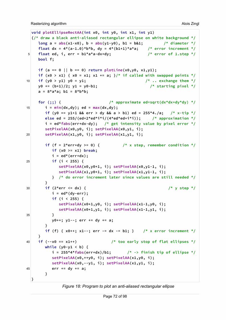
Rasterizing algorithm Alois Zingl
void plotEllipseRectAA(int x0, int y0, int x1, int y1){/* draw a black anti-aliased rectangular ellipse on white background */ long a = abs(x1-x0), b = abs(y1-y0), b1 = b&1; /* diameter */ float dx = 4*(a-1.0)*b*b, dy = 4*(b1+1)*a*a; /* error increment */ float ed, i, err = b1*a*a-dx+dy; /* error of 1.step */ bool f;
if (a == 0 || b == 0) return plotLine(x0,y0, x1,y1); if (x0 > x1) { x0 = x1; x1 += a; }/* if called with swapped points */ if (y0 > y1) y0 = y1; /* .. exchange them */ y0 += (b+1)/2; y1 = y0-b1; /* starting pixel */ a = 8*a*a; b1 = 8*b*b;
for (;;) { /* approximate ed=sqrt(dx*dx+dy*dy) */ i = min(dx,dy); ed = max(dx,dy); if (y0 == y1+1 && err > dy && a > b1) ed = 255*4./a; /* x-tip */ else ed = 255/(ed+2*ed*i*i/(4*ed*ed+i*i)); /* approximation */ i = ed*fabs(err+dx-dy); /* get intensity value by pixel error */ setPixelAA(x0,y0, i); setPixelAA(x0,y1, i); setPixelAA(x1,y0, i); setPixelAA(x1,y1, i); if (f = 2*err+dy >= 0) { /* x step, remember condition */ if (x0 >= x1) break; i = ed*(err+dx); if (i < 255) { setPixelAA(x0,y0+1, i); setPixelAA(x0,y1-1, i); setPixelAA(x1,y0+1, i); setPixelAA(x1,y1-1, i); } /* do error increment later since values are still needed */ } if (2*err <= dx) { /* y step */ i = ed*(dy-err); if (i < 255) { setPixelAA(x0+1,y0, i); setPixelAA(x1-1,y0, i); setPixelAA(x0+1,y1, i); setPixelAA(x1-1,y1, i); } y0++; y1--; err += dy += a; } if (f) { x0++; x1--; err -= dx -= b1; } /* x error increment */ } if (--x0 == x1++) /* too early stop of flat ellipses */ while (y0-y1 < b) { i = 255*4*fabs(err+dx)/b1; /* -> finish tip of ellipse */ setPixelAA(x0,++y0, i); setPixelAA(x1,y0, i); setPixelAA(x0,--y1, i); setPixelAA(x1,y1, i); err += dy += a; }}
Figure 18: Program to plot an anti-aliased rectangular ellipse
Page 72 of 98
5
10
15
20
25
30
35
40
45

Rasterizing algorithm Alois Zingl
The maximum error value of the tip of flat ellipses is difficult to define.
Figure 28: Example of an anti-aliased ellipse
A rotated ellipse could be drawn by using the anti-aliased rational quadratic Bézier curve of
chapter 7.6.
7.4 Anti-aliased quadratic Bézier curveThe main procedure for drawing the anti-aliased quadratic Bézier curve remains the same
as in chapter 3.7 listing 10. Only the subroutine for the Bézier segment changes slightly to
set the pixel intensity of the curve according to the error value.
Figure 29: Example of an anti-aliased quadratic Bézier curve
The calculation of the maximum error distance also depends on the position. It makes a
difference if the values of the current or next pixel are used. An exact calculation needs
additionally the derivative of the curve. Using the difference values is an concession to get
a faster and simpler algorithm.
Another slight error is introduced if the algorithm fails due to the other part of the curve
comes close. In such case the curve is finished by an anti-aliased line but the transition
from the curve to the line could not be exact. In addition the anti-aliased pixel values of the
line to not exactly correspond to the values resulting from the Bézier curve calculation.
Page 73 of 98
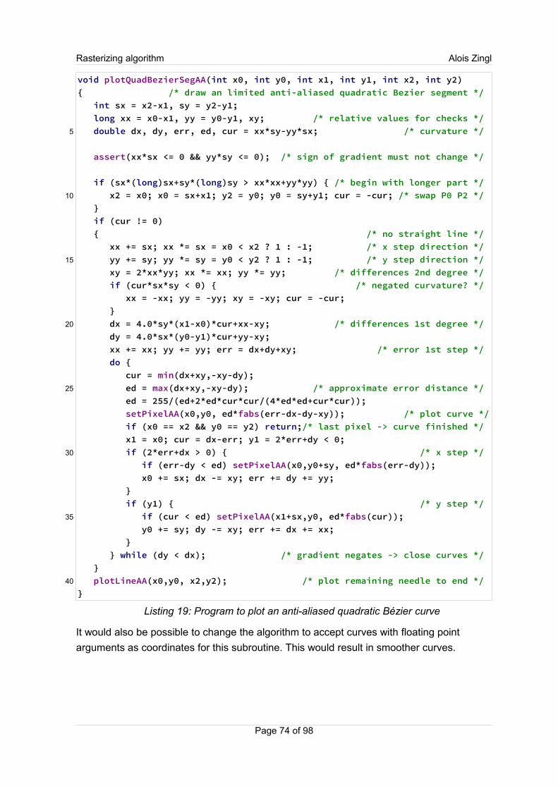
Rasterizing algorithm Alois Zingl
void plotQuadBezierSegAA(int x0, int y0, int x1, int y1, int x2, int y2){ /* draw an limited anti-aliased quadratic Bezier segment */ int sx = x2-x1, sy = y2-y1; long xx = x0-x1, yy = y0-y1, xy; /* relative values for checks */ double dx, dy, err, ed, cur = xx*sy-yy*sx; /* curvature */
assert(xx*sx <= 0 && yy*sy <= 0); /* sign of gradient must not change */
if (sx*(long)sx+sy*(long)sy > xx*xx+yy*yy) { /* begin with longer part */ x2 = x0; x0 = sx+x1; y2 = y0; y0 = sy+y1; cur = -cur; /* swap P0 P2 */ } if (cur != 0) { /* no straight line */ xx += sx; xx *= sx = x0 < x2 ? 1 : -1; /* x step direction */ yy += sy; yy *= sy = y0 < y2 ? 1 : -1; /* y step direction */ xy = 2*xx*yy; xx *= xx; yy *= yy; /* differences 2nd degree */ if (cur*sx*sy < 0) { /* negated curvature? */ xx = -xx; yy = -yy; xy = -xy; cur = -cur; } dx = 4.0*sy*(x1-x0)*cur+xx-xy; /* differences 1st degree */ dy = 4.0*sx*(y0-y1)*cur+yy-xy; xx += xx; yy += yy; err = dx+dy+xy; /* error 1st step */ do { cur = min(dx+xy,-xy-dy); ed = max(dx+xy,-xy-dy); /* approximate error distance */ ed = 255/(ed+2*ed*cur*cur/(4*ed*ed+cur*cur)); setPixelAA(x0,y0, ed*fabs(err-dx-dy-xy)); /* plot curve */ if (x0 == x2 && y0 == y2) return;/* last pixel -> curve finished */ x1 = x0; cur = dx-err; y1 = 2*err+dy < 0; if (2*err+dx > 0) { /* x step */ if (err-dy < ed) setPixelAA(x0,y0+sy, ed*fabs(err-dy)); x0 += sx; dx -= xy; err += dy += yy; } if (y1) { /* y step */ if (cur < ed) setPixelAA(x1+sx,y0, ed*fabs(cur)); y0 += sy; dy -= xy; err += dx += xx; } } while (dy < dx); /* gradient negates -> close curves */ } plotLineAA(x0,y0, x2,y2); /* plot remaining needle to end */}
Listing 19: Program to plot an anti-aliased quadratic Bézier curve
It would also be possible to change the algorithm to accept curves with floating point
arguments as coordinates for this subroutine. This would result in smoother curves.
Page 74 of 98
5
10
15
20
25
30
35
40
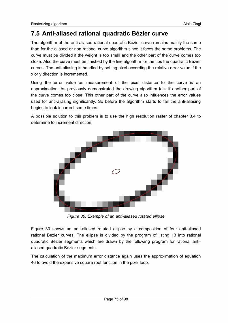
Rasterizing algorithm Alois Zingl
7.5 Anti-aliased rational quadratic Bézier curveThe algorithm of the anti-aliased rational quadratic Bézier curve remains mainly the same
than for the aliased or non rational curve algorithm since it faces the same problems. The
curve must be divided if the weight is too small and the other part of the curve comes too
close. Also the curve must be finished by the line algorithm for the tips the quadratic Bézier
curves. The anti-aliasing is handled by setting pixel according the relative error value if the
x or y direction is incremented.
Using the error value as measurement of the pixel distance to the curve is an
approximation. As previously demonstrated the drawing algorithm fails if another part of
the curve comes too close. This other part of the curve also influences the error values
used for anti-aliasing significantly. So before the algorithm starts to fail the anti-aliasing
begins to look incorrect some times.
A possible solution to this problem is to use the high resolution raster of chapter 3.4 to
determine to increment direction.
Figure 30: Example of an anti-aliased rotated ellipse
Figure 30 shows an anti-aliased rotated ellipse by a composition of four anti-aliased
rational Bézier curves. The ellipse is divided by the program of listing 13 into rational
quadratic Bézier segments which are drawn by the following program for rational anti-
aliased quadratic Bézier segments.
The calculation of the maximum error distance again uses the approximation of equation
46 to avoid the expensive square root function in the pixel loop.
Page 75 of 98

Rasterizing algorithm Alois Zingl
void plotQuadRationalBezierSegAA(int x0, int y0, int x1, int y1, int x2, int y2, float w){ /* draw an anti-aliased rational quadratic Bezier segment, squared weight */ int sx = x2-x1, sy = y2-y1; /* relative values for checks */ double dx = x0-x2, dy = y0-y2, xx = x0-x1, yy = y0-y1; double xy = xx*sy+yy*sx, cur = xx*sy-yy*sx, err, ed; /* curvature */ bool f;
assert(xx*sx <= 0.0 && yy*sy <= 0.0); /* sign of gradient must not change */
if (cur != 0.0 && w > 0.0) { /* no straight line */ if (sx*(long)sx+sy*(long)sy > xx*xx+yy*yy) { /* begin with longer part */ x2 = x0; x0 -= dx; y2 = y0; y0 -= dy; cur = -cur; /* swap P0 P2 */ } xx = 2.0*(4.0*w*sx*xx+dx*dx); /* differences 2nd degree */ yy = 2.0*(4.0*w*sy*yy+dy*dy); sx = x0 < x2 ? 1 : -1; /* x step direction */ sy = y0 < y2 ? 1 : -1; /* y step direction */ xy = -2.0*sx*sy*(2.0*w*xy+dx*dy);
if (cur*sx*sy < 0) { /* negated curvature? */ xx = -xx; yy = -yy; cur = -cur; xy = -xy; } dx = 4.0*w*(x1-x0)*sy*cur+xx/2.0+xy; /* differences 1st degree */ dy = 4.0*w*(y0-y1)*sx*cur+yy/2.0+xy;
if (w < 0.5 && dy > dx) { /* flat ellipse, algorithm fails */ cur = (w+1.0)/2.0; w = sqrt(w); xy = 1.0/(w+1.0); sx = floor((x0+2.0*w*x1+x2)*xy/2.0+0.5); /* subdivide curve in half */ sy = floor((y0+2.0*w*y1+y2)*xy/2.0+0.5); dx = floor((w*x1+x0)*xy+0.5); dy = floor((y1*w+y0)*xy+0.5); plotQuadRationalBezierSegAA(x0,y0, dx,dy, sx,sy, cur); /* plot apart */ dx = floor((w*x1+x2)*xy+0.5); dy = floor((y1*w+y2)*xy+0.5); return plotQuadRationalBezierSegAA(sx,sy, dx,dy, x2,y2, cur); } err = dx+dy-xy; /* error 1st step */ do { /* pixel loop */ cur = min(dx-xy,xy-dy); ed = max(dx-xy,xy-dy); ed += 2*ed*cur*cur/(4.*ed*ed+cur*cur); /* approximate error distance */ x1 = 255*abs(err-dx-dy+xy)/ed; /* get blend value by pixel error */ if (x1 < 256) setPixelAA(x0,y0, x1); /* plot curve */ if (f = 2*err+dy < 0) { /* y step */ if (y0 == y2) return; /* last pixel -> curve finished */ if (dx-err < ed) setPixelAA(x0+sx,y0, 255*fabs(dx-err)/ed); } if (2*err+dx > 0) { /* x step */ if (x0 == x2) return; /* last pixel -> curve finished */ if (err-dy < ed) setPixelAA(x0,y0+sy, 255*fabs(err-dy)/ed); x0 += sx; dx += xy; err += dy += yy; } if (f) { y0 += sy; dy += xy; err += dx += xx; } /* y step */ } while (dy < dx); /* gradient negates -> algorithm fails */ } plotLineAA(x0,y0, x2,y2); /* plot remaining needle to end */}
Listing 20: Program to plot an anti-aliased rational quadratic Bézier curve
Page 76 of 98
5
10
15
20
25
30
35
40
45
50
55
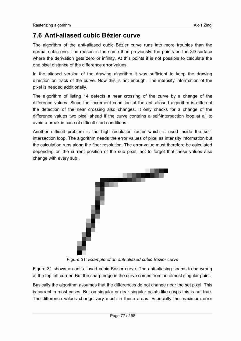
Rasterizing algorithm Alois Zingl
7.6 Anti-aliased cubic Bézier curveThe algorithm of the anti-aliased cubic Bézier curve runs into more troubles than the
normal cubic one. The reason is the same than previously: the points on the 3D surface
where the derivation gets zero or infinity. At this points it is not possible to calculate the
one pixel distance of the difference error values.
In the aliased version of the drawing algorithm it was sufficient to keep the drawing
direction on track of the curve. Now this is not enough. The intensity information of the
pixel is needed additionally.
The algorithm of listing 14 detects a near crossing of the curve by a change of the
difference values. Since the increment condition of the anti-aliased algorithm is different
the detection of the near crossing also changes. It only checks for a change of the
difference values two pixel ahead if the curve contains a self-intersection loop at all to
avoid a break in case of difficult start conditions.
Another difficult problem is the high resolution raster which is used inside the self-
intersection loop. The algorithm needs the error values of pixel as intensity information but
the calculation runs along the finer resolution. The error value must therefore be calculated
depending on the current position of the sub pixel, not to forget that these values also
change with every sub .
Figure 31: Example of an anti-aliased cubic Bézier curve
Figure 31 shows an anti-aliased cubic Bézier curve. The anti-aliasing seems to be wrong
at the top left corner. But the sharp edge in the curve comes from an almost singular point.
Basically the algorithm assumes that the differences do not change near the set pixel. This
is correct in most cases. But on singular or near singular points like cusps this is not true.
The difference values change very much in these areas. Especially the maximum error
Page 77 of 98
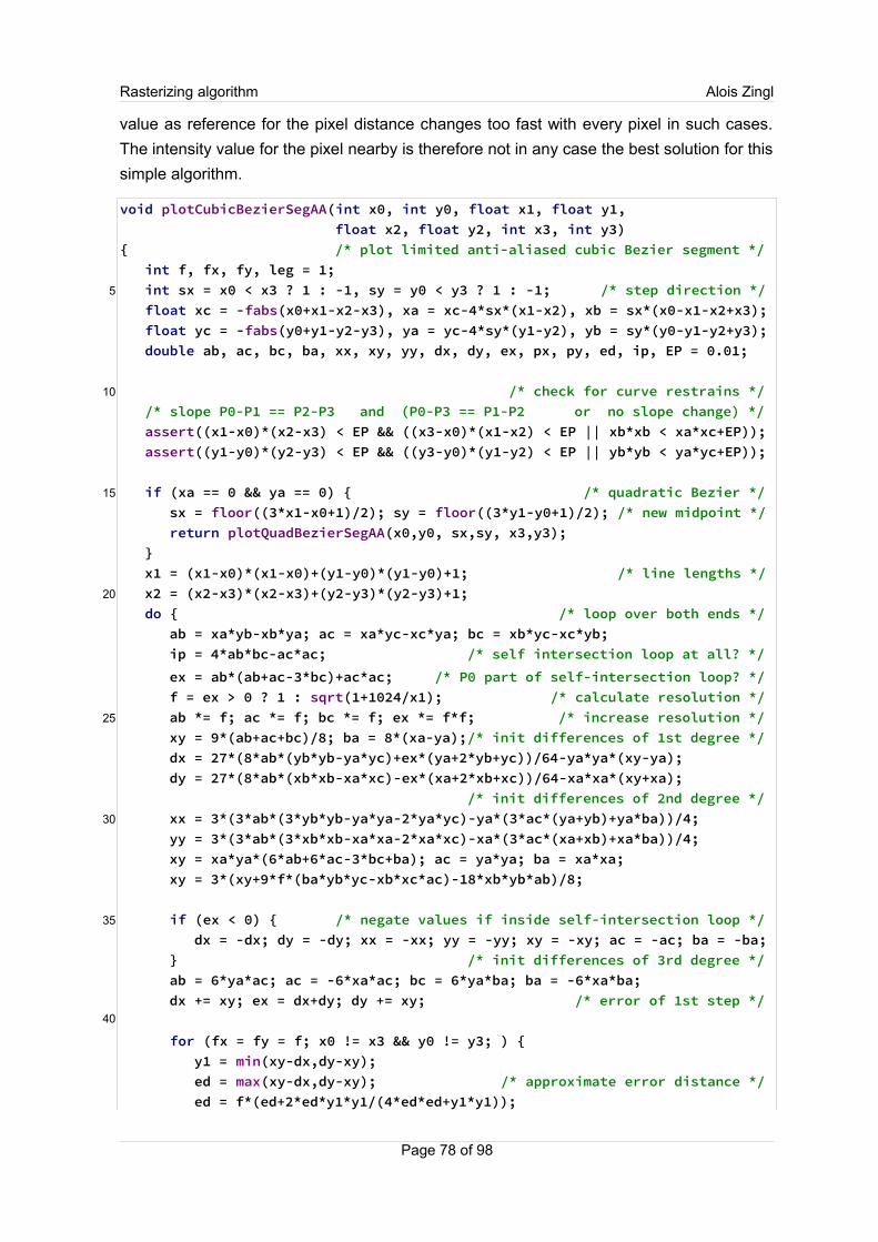
Rasterizing algorithm Alois Zingl
value as reference for the pixel distance changes too fast with every pixel in such cases.
The intensity value for the pixel nearby is therefore not in any case the best solution for this
simple algorithm.
void plotCubicBezierSegAA(int x0, int y0, float x1, float y1, float x2, float y2, int x3, int y3) { /* plot limited anti-aliased cubic Bezier segment */ int f, fx, fy, leg = 1; int sx = x0 < x3 ? 1 : -1, sy = y0 < y3 ? 1 : -1; /* step direction */ float xc = -fabs(x0+x1-x2-x3), xa = xc-4*sx*(x1-x2), xb = sx*(x0-x1-x2+x3); float yc = -fabs(y0+y1-y2-y3), ya = yc-4*sy*(y1-y2), yb = sy*(y0-y1-y2+y3); double ab, ac, bc, ba, xx, xy, yy, dx, dy, ex, px, py, ed, ip, EP = 0.01; /* check for curve restrains */ /* slope P0-P1 == P2-P3 and (P0-P3 == P1-P2 or no slope change) */ assert((x1-x0)*(x2-x3) < EP && ((x3-x0)*(x1-x2) < EP || xb*xb < xa*xc+EP)); assert((y1-y0)*(y2-y3) < EP && ((y3-y0)*(y1-y2) < EP || yb*yb < ya*yc+EP));
if (xa == 0 && ya == 0) { /* quadratic Bezier */ sx = floor((3*x1-x0+1)/2); sy = floor((3*y1-y0+1)/2); /* new midpoint */ return plotQuadBezierSegAA(x0,y0, sx,sy, x3,y3); } x1 = (x1-x0)*(x1-x0)+(y1-y0)*(y1-y0)+1; /* line lengths */ x2 = (x2-x3)*(x2-x3)+(y2-y3)*(y2-y3)+1; do { /* loop over both ends */ ab = xa*yb-xb*ya; ac = xa*yc-xc*ya; bc = xb*yc-xc*yb; ip = 4*ab*bc-ac*ac; /* self intersection loop at all? */
ex = ab*(ab+ac-3*bc)+ac*ac; /* P0 part of self-intersection loop? */ f = ex > 0 ? 1 : sqrt(1+1024/x1); /* calculate resolution */ ab *= f; ac *= f; bc *= f; ex *= f*f; /* increase resolution */ xy = 9*(ab+ac+bc)/8; ba = 8*(xa-ya);/* init differences of 1st degree */ dx = 27*(8*ab*(yb*yb-ya*yc)+ex*(ya+2*yb+yc))/64-ya*ya*(xy-ya); dy = 27*(8*ab*(xb*xb-xa*xc)-ex*(xa+2*xb+xc))/64-xa*xa*(xy+xa); /* init differences of 2nd degree */ xx = 3*(3*ab*(3*yb*yb-ya*ya-2*ya*yc)-ya*(3*ac*(ya+yb)+ya*ba))/4; yy = 3*(3*ab*(3*xb*xb-xa*xa-2*xa*xc)-xa*(3*ac*(xa+xb)+xa*ba))/4; xy = xa*ya*(6*ab+6*ac-3*bc+ba); ac = ya*ya; ba = xa*xa; xy = 3*(xy+9*f*(ba*yb*yc-xb*xc*ac)-18*xb*yb*ab)/8;
if (ex < 0) { /* negate values if inside self-intersection loop */ dx = -dx; dy = -dy; xx = -xx; yy = -yy; xy = -xy; ac = -ac; ba = -ba; } /* init differences of 3rd degree */ ab = 6*ya*ac; ac = -6*xa*ac; bc = 6*ya*ba; ba = -6*xa*ba; dx += xy; ex = dx+dy; dy += xy; /* error of 1st step */
for (fx = fy = f; x0 != x3 && y0 != y3; ) { y1 = min(xy-dx,dy-xy); ed = max(xy-dx,dy-xy); /* approximate error distance */ ed = f*(ed+2*ed*y1*y1/(4*ed*ed+y1*y1));
Page 78 of 98
5
10
15
20
25
30
35
40
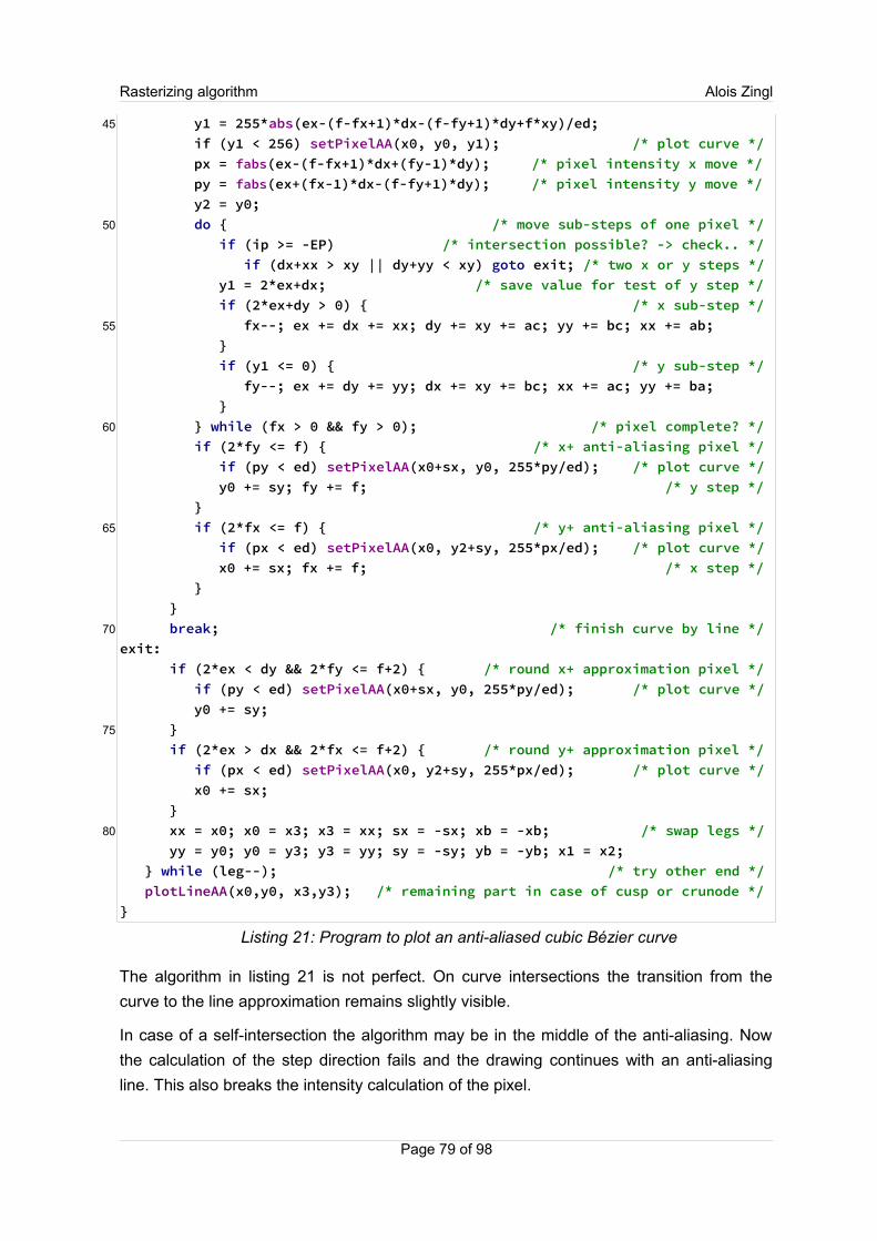
Rasterizing algorithm Alois Zingl
y1 = 255*abs(ex-(f-fx+1)*dx-(f-fy+1)*dy+f*xy)/ed; if (y1 < 256) setPixelAA(x0, y0, y1); /* plot curve */ px = fabs(ex-(f-fx+1)*dx+(fy-1)*dy); /* pixel intensity x move */ py = fabs(ex+(fx-1)*dx-(f-fy+1)*dy); /* pixel intensity y move */ y2 = y0; do { /* move sub-steps of one pixel */ if (ip >= -EP) /* intersection possible? -> check.. */ if (dx+xx > xy || dy+yy < xy) goto exit; /* two x or y steps */ y1 = 2*ex+dx; /* save value for test of y step */ if (2*ex+dy > 0) { /* x sub-step */ fx--; ex += dx += xx; dy += xy += ac; yy += bc; xx += ab; } if (y1 <= 0) { /* y sub-step */ fy--; ex += dy += yy; dx += xy += bc; xx += ac; yy += ba; } } while (fx > 0 && fy > 0); /* pixel complete? */ if (2*fy <= f) { /* x+ anti-aliasing pixel */ if (py < ed) setPixelAA(x0+sx, y0, 255*py/ed); /* plot curve */ y0 += sy; fy += f; /* y step */ } if (2*fx <= f) { /* y+ anti-aliasing pixel */ if (px < ed) setPixelAA(x0, y2+sy, 255*px/ed); /* plot curve */ x0 += sx; fx += f; /* x step */ } } break; /* finish curve by line */exit: if (2*ex < dy && 2*fy <= f+2) { /* round x+ approximation pixel */ if (py < ed) setPixelAA(x0+sx, y0, 255*py/ed); /* plot curve */ y0 += sy; } if (2*ex > dx && 2*fx <= f+2) { /* round y+ approximation pixel */ if (px < ed) setPixelAA(x0, y2+sy, 255*px/ed); /* plot curve */ x0 += sx; } xx = x0; x0 = x3; x3 = xx; sx = -sx; xb = -xb; /* swap legs */ yy = y0; y0 = y3; y3 = yy; sy = -sy; yb = -yb; x1 = x2; } while (leg--); /* try other end */ plotLineAA(x0,y0, x3,y3); /* remaining part in case of cusp or crunode */}
Listing 21: Program to plot an anti-aliased cubic Bézier curve
The algorithm in listing 21 is not perfect. On curve intersections the transition from the
curve to the line approximation remains slightly visible.
In case of a self-intersection the algorithm may be in the middle of the anti-aliasing. Now
the calculation of the step direction fails and the drawing continues with an anti-aliasing
line. This also breaks the intensity calculation of the pixel.
Page 79 of 98
45
50
55
60
65
70
75
80
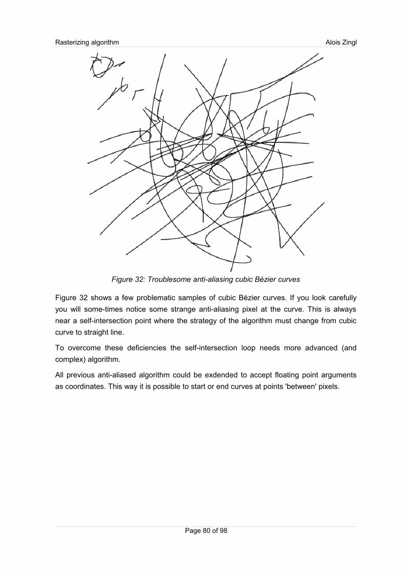
Rasterizing algorithm Alois Zingl
Figure 32: Troublesome anti-aliasing cubic Bézier curves
Figure 32 shows a few problematic samples of cubic Bézier curves. If you look carefully
you will some-times notice some strange anti-aliasing pixel at the curve. This is always
near a self-intersection point where the strategy of the algorithm must change from cubic
curve to straight line.
To overcome these deficiencies the self-intersection loop needs more advanced (and
complex) algorithm.
All previous anti-aliased algorithm could be exdended to accept floating point arguments
as coordinates. This way it is possible to start or end curves at points 'between' pixels.
Page 80 of 98
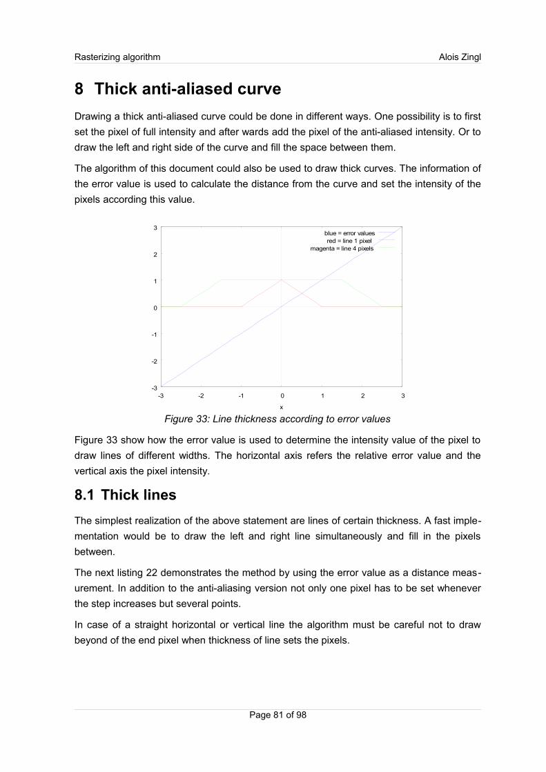
Rasterizing algorithm Alois Zingl
8 Thick anti-aliased curve
Drawing a thick anti-aliased curve could be done in different ways. One possibility is to first
set the pixel of full intensity and after wards add the pixel of the anti-aliased intensity. Or to
draw the left and right side of the curve and fill the space between them.
The algorithm of this document could also be used to draw thick curves. The information of
the error value is used to calculate the distance from the curve and set the intensity of the
pixels according this value.
Figure 33: Line thickness according to error values
Figure 33 show how the error value is used to determine the intensity value of the pixel to
draw lines of different widths. The horizontal axis refers the relative error value and the
vertical axis the pixel intensity.
8.1 Thick lines
The simplest realization of the above statement are lines of certain thickness. A fast imple-
mentation would be to draw the left and right line simultaneously and fill in the pixels
between.
The next listing 22 demonstrates the method by using the error value as a distance meas-
urement. In addition to the anti-aliasing version not only one pixel has to be set whenever
the step increases but several points.
In case of a straight horizontal or vertical line the algorithm must be careful not to draw
beyond of the end pixel when thickness of line sets the pixels.
Page 81 of 98
-3
-2
-1
0
1
2
3
-3 -2 -1 0 1 2 3
x
blue = error valuesred = line 1 pixel
magenta = line 4 pixels

Rasterizing algorithm Alois Zingl
void plotLineWidth(int x0, int y0, int x1, int y1, float wd){ /* plot an anti-aliased line of width wd */ int dx = abs(x1-x0), sx = x0 < x1 ? 1 : -1; int dy = abs(y1-y0), sy = y0 < y1 ? 1 : -1; int err = dx-dy, e2, x2, y2; /* error value e_xy */ float ed = dx+dy == 0 ? 1 : sqrt((float)dx*dx+(float)dy*dy); for (wd = (wd+1)/2; ; ) { /* pixel loop */ setPixelColor(x0, y0, max(0,255*(abs(err-dx+dy)/ed-wd+1))); e2 = err; x2 = x0; if (2*e2 >= -dx) { /* x step */ for (e2 += dy, y2 = y0; e2 < ed*wd && (y1 != y2 || dx > dy); e2 += dx) setPixelColor(x0, y2 += sy, max(0,255*(abs(e2)/ed-wd+1))); if (x0 == x1) break; e2 = err; err -= dy; x0 += sx; } if (2*e2 <= dy) { /* y step */ for (e2 = dx-e2; e2 < ed*wd && (x1 != x2 || dx < dy); e2 += dy) setPixelColor(x2 += sx, y0, max(0,255*(abs(e2)/ed-wd+1))); if (y0 == y1) break; err += dx; y0 += sy; } }}
Listing 22: Program to plot an anti-aliased thick line
Curves of thick lines need special attention at the end points. The type of the end points
mostly depend on the application. Different possibilities are flat, rectangle, round, arrows or
special customized. This is also important if the line is continued either by another line
another type of curve like arcs, or Bézier curves of higher degree. It is therefore not
possible to present a universal algorithm for all types. None the less an adaption to
different requirements should be possible.
Figure 34: Thick line with anti-aliasing
Page 82 of 98
5
10
15
20

Rasterizing algorithm Alois Zingl
8.2 Thick curves of higher degree
The previous algorithm could also be applied to curves of higher degree. This works
straight forward as long as no other curve comes close. Since this type of algorithm used
the error values farther away from the curve itself the assumption that the difference values
do not change will fail more likely. It gets therefore very difficult to draw more complex
curves with sharp edges, intersections and loops. Whenever another part of the curve
comes too close the differences change too much and more advanced techniques must be
used to compensate the flaw.
For simple figures like circles and ellipses it is easier to draw the inner and outer edge of
the curve and fill in the space between.
Page 83 of 98
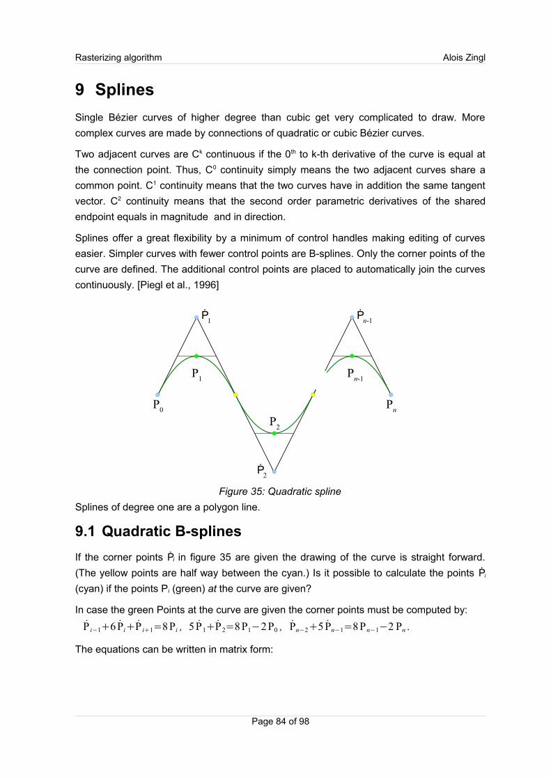
Rasterizing algorithm Alois Zingl
9 Splines
Single Bézier curves of higher degree than cubic get very complicated to draw. More
complex curves are made by connections of quadratic or cubic Bézier curves.
Two adjacent curves are Ck continuous if the 0th to k-th derivative of the curve is equal at
the connection point. Thus, C0 continuity simply means the two adjacent curves share a
common point. C1 continuity means that the two curves have in addition the same tangent
vector. C2 continuity means that the second order parametric derivatives of the shared
endpoint equals in magnitude and in direction.
Splines offer a great flexibility by a minimum of control handles making editing of curves
easier. Simpler curves with fewer control points are B-splines. Only the corner points of the
curve are defined. The additional control points are placed to automatically join the curves
continuously. [Piegl et al., 1996]
Splines of degree one are a polygon line.
9.1 Quadratic B-splines
If the corner points Ṗi in figure 35 are given the drawing of the curve is straight forward.
(The yellow points are half way between the cyan.) Is it possible to calculate the points Ṗi
(cyan) if the points Pi (green) at the curve are given?
In case the green Points at the curve are given the corner points must be computed by:
P i−16 PiP i1=8Pi , 5 P1P2=8P1−2P0 , Pn−25 Pn−1=8Pn−1−2 Pn .
The equations can be written in matrix form:
Page 84 of 98
Figure 35: Quadratic spline
P0
Ṗ1
Ṗ2
Ṗn-1
Pn
P1
P2
Pn-1

Rasterizing algorithm Alois Zingl
[5 1 01 6 1⋱ ⋱ ⋱
1 6 10 1 5
]⋅[P1
P2
⋮Pn−2
Pn−1
]=[8P1 −2 P0
8P2
⋮8Pn−2
8Pn−1−2Pn
] (47)
This tridiagonal systems of linear equations could be solved by the Thomas algorithm in(n) operations by LU decomposition of the matrix A·x = d [Thomas, 1949]:
[a1 b1 0c2 a2 b2
⋱ ⋱ ⋱cn−1 an−1 bn−1
0 cn an
][x1
x2
⋮xn−1
xn
]==[
1 0l 2 1⋱ ⋱
l n−1 10 l n 1
]⋅[m1 b1 0
m2 b2
⋱ ⋱mn−1 bn−1
0 mn
][x1
x2
⋮xn−1
xn
]=[d 1
d 2
⋮d n−1
d n
](48)
The matrix equation is now solved by the steps: L·U·x = d, L·y = d and U·x = y.
Comparing the terms the unknowns could be calculated by a forward sweep:
m1 = a1 , li+1 = ci+1 /mi , mi+1 = ai+1 – bi li+1 and the temporary result y1 = d1, yi = di – yi–1 li.
The back substitution finally calculates the desired result: xn = yn /mn , xi–1 = (yi–1 – bi–1 xi)/mi–1.
If the input arrays could be used as temporary buffer no extra storage is needed by the
algorithm. If this is not desirable new arrays must be allocated to store the intermediate
results.
Page 85 of 98
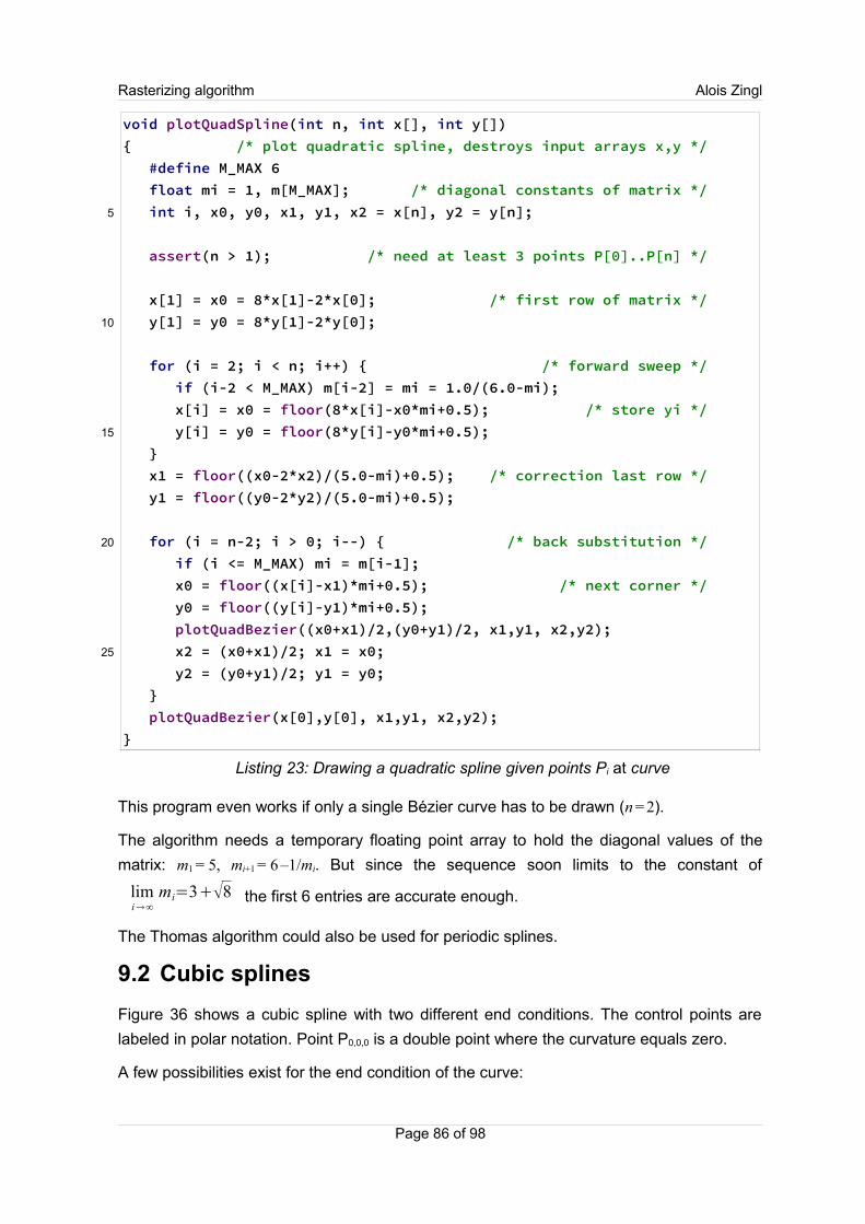
Rasterizing algorithm Alois Zingl
void plotQuadSpline(int n, int x[], int y[]){ /* plot quadratic spline, destroys input arrays x,y */ #define M_MAX 6 float mi = 1, m[M_MAX]; /* diagonal constants of matrix */ int i, x0, y0, x1, y1, x2 = x[n], y2 = y[n];
assert(n > 1); /* need at least 3 points P[0]..P[n] */
x[1] = x0 = 8*x[1]-2*x[0]; /* first row of matrix */ y[1] = y0 = 8*y[1]-2*y[0];
for (i = 2; i < n; i++) { /* forward sweep */ if (i-2 < M_MAX) m[i-2] = mi = 1.0/(6.0-mi); x[i] = x0 = floor(8*x[i]-x0*mi+0.5); /* store yi */ y[i] = y0 = floor(8*y[i]-y0*mi+0.5); } x1 = floor((x0-2*x2)/(5.0-mi)+0.5); /* correction last row */ y1 = floor((y0-2*y2)/(5.0-mi)+0.5);
for (i = n-2; i > 0; i--) { /* back substitution */ if (i <= M_MAX) mi = m[i-1]; x0 = floor((x[i]-x1)*mi+0.5); /* next corner */ y0 = floor((y[i]-y1)*mi+0.5); plotQuadBezier((x0+x1)/2,(y0+y1)/2, x1,y1, x2,y2); x2 = (x0+x1)/2; x1 = x0; y2 = (y0+y1)/2; y1 = y0; } plotQuadBezier(x[0],y[0], x1,y1, x2,y2);}
Listing 23: Drawing a quadratic spline given points Pi at curve
This program even works if only a single Bézier curve has to be drawn (n = 2).
The algorithm needs a temporary floating point array to hold the diagonal values of the
matrix: m1 = 5, mi+1 = 6 –1/mi. But since the sequence soon limits to the constant of
limi∞
mi=38 the first 6 entries are accurate enough.
The Thomas algorithm could also be used for periodic splines.
9.2 Cubic splines
Figure 36 shows a cubic spline with two different end conditions. The control points are
labeled in polar notation. Point P0,0,0 is a double point where the curvature equals zero.
A few possibilities exist for the end condition of the curve:
Page 86 of 98
5
10
15
20
25

Rasterizing algorithm Alois Zingl
• open end: the curve is just drawn from P1,1,1 to Pn-1,n-1,n-1.
• tangent: the curvature at the end points P0,0,0 and Pn,n,n vanishes.
• periodic: the curve is closed by P0,0,0 = Pn,n,n.
In case the corner points (cyan) are given the curve could be subdivided in cubic Bézier
curves using DeBoor's algorithm. A cubic Bézier curve is extracted by the Points P i,i,i-Pi,i,i+1-
Pi,i+1,i+1-Pi+1,i+1,i+1. The line Pi-1,i,i+1-Pi,i+1,i+2 is made thirds to get Pi,i,i+1 and Pi,i+1,i+1. The line Pi-1,i,i-
Pi,i,i+1 is halved to get Pi,i,i.
The equations for cubic splines are similar:
P i−14 PiPi1=6 Pi , 7 P12 P2=12P1−3P0 , 2 Pn−27 Pn−1=12Pn−1−3 Pn .
[7 2 02 8 2⋱ ⋱ ⋱
2 8 20 2 7
]⋅[P1
P2
⋮Pn−2
Pn−1
]=[12 P1 −3P0
12 P2
⋮12 Pn−2
12 Pn−1−3Pn
] (49)
In case the through points (yellow) are given it is again possible to compute the corner
points. But this system of linear equations has two degrees of freedom. A possible condi-
tion for the needed restriction is to define the curvature at both ends to be zero (multiple
knots): B''(0) = 0. This condition is shown at the beginning of the curve in figure 36 (P0,0,0).
Page 87 of 98
Figure 36: Cubic spline
P0,0,0
=P0,0,1
Ṗ0,1,2
Ṗ1,2,3
Pn,n,n
P1,1,1 P
2,2,2
Pn-1,n-1,n-1
P3,3,3
Ṗ2,3,4
Ṗn-2,n-1,n
P1,2,2
P1,1,2
P0,1,1
P2,2,3
P2,3,3
Ṗn-1,n,n
Pn-1,n-1,n
Pn-2,n-1,n-1
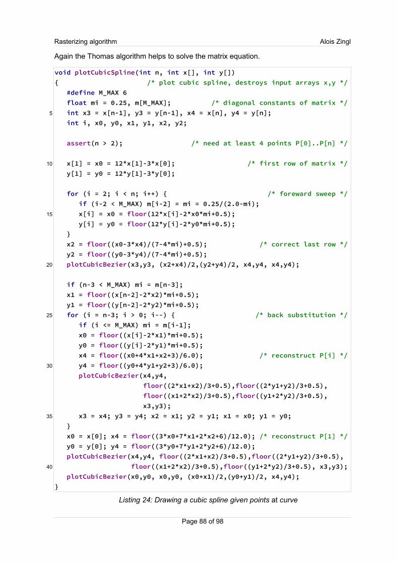
Rasterizing algorithm Alois Zingl
Again the Thomas algorithm helps to solve the matrix equation.
void plotCubicSpline(int n, int x[], int y[]){ /* plot cubic spline, destroys input arrays x,y */ #define M_MAX 6 float mi = 0.25, m[M_MAX]; /* diagonal constants of matrix */ int x3 = x[n-1], y3 = y[n-1], x4 = x[n], y4 = y[n]; int i, x0, y0, x1, y1, x2, y2;
assert(n > 2); /* need at least 4 points P[0]..P[n] */
x[1] = x0 = 12*x[1]-3*x[0]; /* first row of matrix */ y[1] = y0 = 12*y[1]-3*y[0];
for (i = 2; i < n; i++) { /* foreward sweep */ if (i-2 < M_MAX) m[i-2] = mi = 0.25/(2.0-mi); x[i] = x0 = floor(12*x[i]-2*x0*mi+0.5); y[i] = y0 = floor(12*y[i]-2*y0*mi+0.5); } x2 = floor((x0-3*x4)/(7-4*mi)+0.5); /* correct last row */ y2 = floor((y0-3*y4)/(7-4*mi)+0.5); plotCubicBezier(x3,y3, (x2+x4)/2,(y2+y4)/2, x4,y4, x4,y4);
if (n-3 < M_MAX) mi = m[n-3]; x1 = floor((x[n-2]-2*x2)*mi+0.5); y1 = floor((y[n-2]-2*y2)*mi+0.5); for (i = n-3; i > 0; i--) { /* back substitution */ if (i <= M_MAX) mi = m[i-1]; x0 = floor((x[i]-2*x1)*mi+0.5); y0 = floor((y[i]-2*y1)*mi+0.5); x4 = floor((x0+4*x1+x2+3)/6.0); /* reconstruct P[i] */ y4 = floor((y0+4*y1+y2+3)/6.0); plotCubicBezier(x4,y4, floor((2*x1+x2)/3+0.5),floor((2*y1+y2)/3+0.5), floor((x1+2*x2)/3+0.5),floor((y1+2*y2)/3+0.5), x3,y3); x3 = x4; y3 = y4; x2 = x1; y2 = y1; x1 = x0; y1 = y0; } x0 = x[0]; x4 = floor((3*x0+7*x1+2*x2+6)/12.0); /* reconstruct P[1] */ y0 = y[0]; y4 = floor((3*y0+7*y1+2*y2+6)/12.0); plotCubicBezier(x4,y4, floor((2*x1+x2)/3+0.5),floor((2*y1+y2)/3+0.5), floor((x1+2*x2)/3+0.5),floor((y1+2*y2)/3+0.5), x3,y3); plotCubicBezier(x0,y0, x0,y0, (x0+x1)/2,(y0+y1)/2, x4,y4);}
Listing 24: Drawing a cubic spline given points at curve
Page 88 of 98
5
10
15
20
25
30
35
40

Rasterizing algorithm Alois Zingl
The algorithm needs an additional floating point array to store the values of the forward
sweep since the curve points are still needed to draw the computed Bézier segment. But
the original points could be reconstructed by the next corner point avoiding the additional
array.
Please note that the cubic spline of size n = 3 drawn with this algorithm is not the same
than a single cubic Bézier although both are defined by 4 points. But the condition for this
spline is in addition to have end points without a curvature, whereas the cubic Bézier does
not have such a restriction.
Page 89 of 98

Rasterizing algorithm Alois Zingl
10ConclusionsRasterizing is a fundamental task in computer graphics. This document reworks the
Bresenham algorithm and extends it for other curves like ellipses and Bézier curves of
quadratic and cubic degree. Generally the algorithm could be used to rasterize any
geometric curve.
10.1 Algorithm to plot implicit equations
The calculations of the previous chapters help to define a common algorithm for the plot-
ting curves of the implicit equation f x , y =0.
1. Since the plotting algorithm relies on a continuously positive or negative gradient the
curve must be subdivided at stationary points at which the gradient changes its sign (or
possibly at self intersections).
The change of the direction could also be included in the pixel loop. The subdivision is
not necessary as long as the curve turn only occurs in one direction at the same time
(either x or y). A change in the direction could be detected by a sign change of the
differences. The increment values are adapted according the new direction. This solu-
tion only runs into troubles if both drawing directions change simultaneously since it
cannot decide which of the curves to follow.
2. The step increment is computed by successive differences of the implicit equation:
in x-direction: dx,y += dx+1,y, err += d10 and in y-direction: dx,y += dx,y+1, err += d01.
3. These increments are initialized by the differences of the starting pixel.
The differences of the error values (of spacing h) are the finite m-th order forward differ-
ences in two dimensions:
d nx n y=
1
hxnx hy
n y∑i x=0
nx
∑iy=0
n y
−1i xi ynx
i xny
i yf xnx−i xhx , yn y−i y h y [nxny=m ].
The initialization value of the polynomial equation of degree n makes the n-th deriv-
ative of the implicit equation: d nx , n y=∂
n f∂ xn x∂ yny
[nxny=n] .
4. The algorithm must take special care if another part of the function comes close to the
set pixel of the curve.
The algorithm could be used on all functions with implicit polynomial equation.
10.2 Algorithm complexity
Since any continuous function can be approximated by a polynomial function (Weierstrass
theorem) this document provides an algorithm to draw any function nearly as fast as a line.
More complex curves only need more additions per pixel.
Page 90 of 98
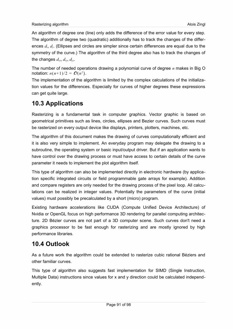
Rasterizing algorithm Alois Zingl
An algorithm of degree one (line) only adds the difference of the error value for every step.
The algorithm of degree two (quadratic) additionally has to track the changes of the differ-
ences dx, dy. (Ellipses and circles are simpler since certain differences are equal due to the
symmetry of the curve.) The algorithm of the third degree also has to track the changes of
the changes dxx, dxy, dyy.
The number of needed operations drawing a polynomial curve of degree n makes in Big O notation: n(n+1)/2 = (n 2) .
The implementation of the algorithm is limited by the complex calculations of the initializa-
tion values for the differences. Especially for curves of higher degrees these expressions
can get quite large.
10.3 Applications
Rasterizing is a fundamental task in computer graphics. Vector graphic is based on
geometrical primitives such as lines, circles, ellipses and Bezier curves. Such curves must
be rasterized on every output device like displays, printers, plotters, machines, etc.
The algorithm of this document makes the drawing of curves computationally efficient and
it is also very simple to implement. An everyday program may delegate the drawing to a
subroutine, the operating system or basic input/output driver. But if an application wants to
have control over the drawing process or must have access to certain details of the curve
parameter it needs to implement the plot algorithm itself.
This type of algorithm can also be implemented directly in electronic hardware (by applica-
tion specific integrated circuits or field programmable gate arrays for example). Addition
and compare registers are only needed for the drawing process of the pixel loop. All calcu-
lations can be realized in integer values. Potentially the parameters of the curve (initial
values) must possibly be precalculated by a short (micro) program.
Existing hardware accelerations like CUDA (Compute Unified Device Architecture) of
Nvidia or OpenGL focus on high performance 3D rendering for parallel computing architec-
ture. 2D Bézier curves are not part of a 3D computer scene. Such curves don't need a
graphics processor to be fast enough for rasterizing and are mostly ignored by high
performance libraries.
10.4 Outlook
As a future work the algorithm could be extended to rasterize cubic rational Béziers and
other familiar curves.
This type of algorithm also suggests fast implementation for SIMD (Single Instruction,
Multiple Data) instructions since values for x and y direction could be calculated independ-
ently.
Page 91 of 98

Rasterizing algorithm Alois Zingl
10.5 Source code
The examples of this documents are available by public at the internet. The web address
is: http://members.chello.at/easyfilter/bresenham.html
The programs have no copyright and could be used and modified by anyone as wanted.
The source code was carefully tested but are given without warranty of any kind. Use it at
your own risk.
Page 92 of 98
Rasterizing algorithm Alois Zingl
Bibliography
[Bézier, 1986] Pierre Étienne Bezier: The Mathematical Basis of the UNISURF CAD
System; Butterworths, London, 1986.
[Bézout, 1764] Étienne Bézout: Recherches sur les degrés des équations résultantes de
l'évanouissement des inconnues et sur les moyens qu'il convient d'employer
pour trouver ces équations; Histoire de l'Académie Royale des Sciences, 1764.
[Bresenham, 1965] Jack E. Bresenham: Algorithms of Computer Control of a Digital
Plotter; IBM System Journal, 1965.
[Casteljau, 1963] Paul de Faget de Casteljau: Courbes et surfaces à pȏles; Technical
report, Citroën, Paris, 1963.
[Cayley, 1857] Arthur Cayley: Note sur la méthode d'élimination de Bezout; Reine Ange-
wandte Mathematik Bd. 53, 366-367, 1857.
[Emeliyanenko, 2007] Pavel Emeliyanenko: Visualization of Points and Segments of Real
Algebraic Plane Curves; Master Thesis, Universität des Saarlandes, Max-
Planck-Insitut für Informatik, 2007.
[Foley, 1995] James David Foley: Computer Graphics, Principles and Practice in C;
Addison-Wesley Professional; 2nd edition,1995.
[Goldman et al., 1985] Ronald N. Goldman, Thomas W. Sederberg: Some applications of
resultants to problems in computational geometry; The Visual Computer,
Volume 1, Number 2, 101-107, 1985.
[Golipour-Koujali, 2005] M. Golipour-Koujali: General Rendering and Antialiasing
Algorithms for Conic Sections; London South Bank University, 2005.
[Loop et al., 2005] Charles Loop, James F. Blinn: Resolution Independent Curve
Rendering using Programmable Graphics Hardware; Association for
Computing Machinery Inc., Microsoft Research, 2005.
[Marsh, 2005] Duncan Marsh: Applied Geometry for Computer Graphics and CAD;
Springer, 2005.
[Piegl et al., 1996] Les Piegl, Wayne Tiller: The NURBS Book; Springer, 1996.
[Ray et al., 2011] Kumar S. Ray, Bimal Kumar Ray: A Method of Deviation for Drawing
Implicit Curves; International Journal of Computer Graphics, Vol. 2, No. 2,
November 2011.
[Sederberg, 2011] Thomas W. Sederberg: Computer Aided Geometric Design Course
Notes; Brigham Young University, http://tom.cs.byu.edu/~557/, 2011.
Page 93 of 98
Rasterizing algorithm Alois Zingl
[Shmakov, 2011] Sergei L. Shmakov: A Universal Method of Solving Quartic Equations;
International Journal of Pure and Applied Mathematics, Volume 71 No. 2, 251-
259.
[Taubin, 1994] Gabriel Taubin: Distance Approximations for Rasterizing Implicit Curves;
IBM Watson Research Center, 1994.
[Thomas, 1949] Llewellyn Hilleth Thomas: Elliptic problems in linear difference equations
over a network; Watson Science Computer Laboratory Report, Columbia
University, New York, 1949.
[Xiaolin, 1991] Xiaolin Wu: An Efficient Antialiasing Technique; University of Western
Ontario, 1991.
[Yang et al., 2000] Hongji Yang, Yang Li, Yong Kui Liu: A Pixel Level Algorithm for
Drawing Curves; Proceedings of the 6th Chinese Automation and Computer
Science Conference in the UK, Loughborough, 2000.
Page 94 of 98
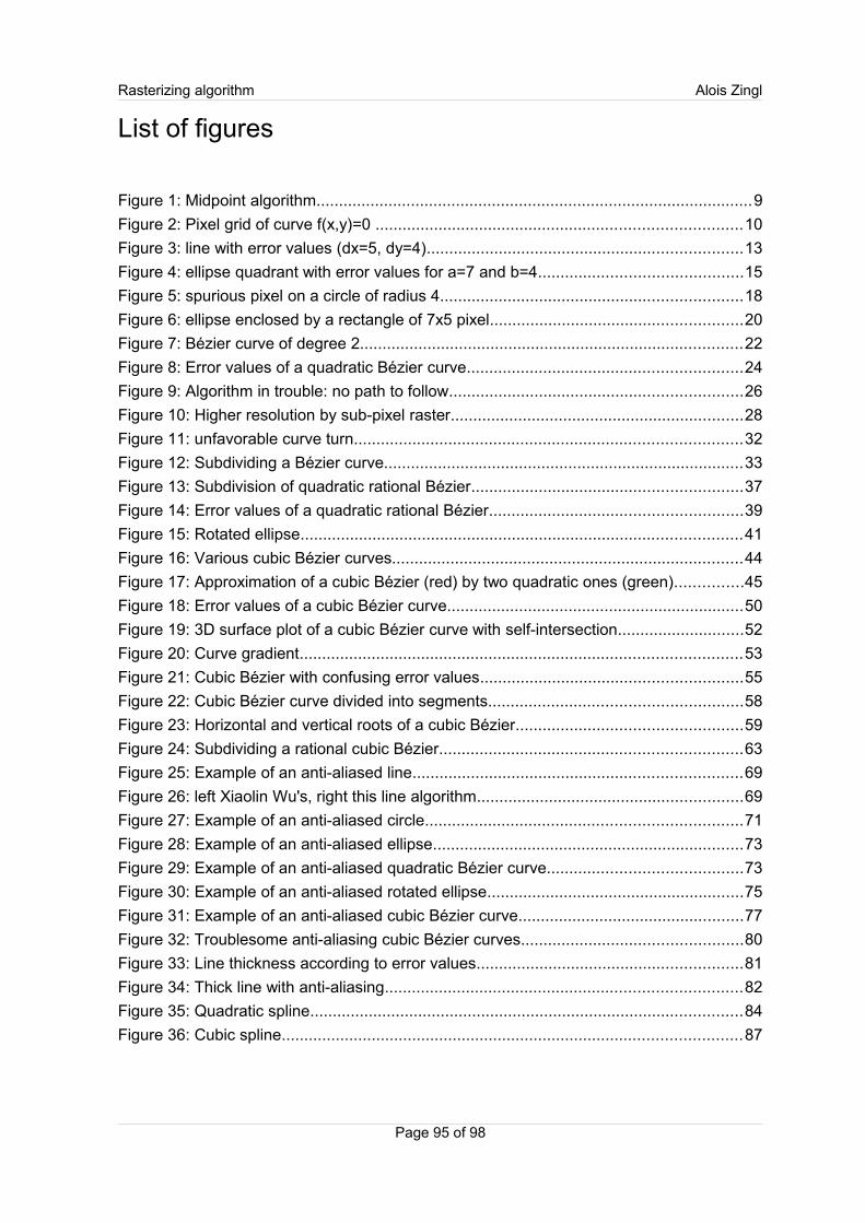
Rasterizing algorithm Alois Zingl
List of figures
Figure 1: Midpoint algorithm.................................................................................................9
Figure 2: Pixel grid of curve f(x,y)=0 .................................................................................10
Figure 3: line with error values (dx=5, dy=4)......................................................................13
Figure 4: ellipse quadrant with error values for a=7 and b=4.............................................15
Figure 5: spurious pixel on a circle of radius 4...................................................................18
Figure 6: ellipse enclosed by a rectangle of 7x5 pixel........................................................20
Figure 7: Bézier curve of degree 2.....................................................................................22
Figure 8: Error values of a quadratic Bézier curve.............................................................24
Figure 9: Algorithm in trouble: no path to follow.................................................................26
Figure 10: Higher resolution by sub-pixel raster.................................................................28
Figure 11: unfavorable curve turn......................................................................................32
Figure 12: Subdividing a Bézier curve................................................................................33
Figure 13: Subdivision of quadratic rational Bézier............................................................37
Figure 14: Error values of a quadratic rational Bézier........................................................39
Figure 15: Rotated ellipse..................................................................................................41
Figure 16: Various cubic Bézier curves..............................................................................44
Figure 17: Approximation of a cubic Bézier (red) by two quadratic ones (green)...............45
Figure 18: Error values of a cubic Bézier curve..................................................................50
Figure 19: 3D surface plot of a cubic Bézier curve with self-intersection............................52
Figure 20: Curve gradient..................................................................................................53
Figure 21: Cubic Bézier with confusing error values..........................................................55
Figure 22: Cubic Bézier curve divided into segments........................................................58
Figure 23: Horizontal and vertical roots of a cubic Bézier..................................................59
Figure 24: Subdividing a rational cubic Bézier...................................................................63
Figure 25: Example of an anti-aliased line.........................................................................69
Figure 26: left Xiaolin Wu's, right this line algorithm...........................................................69
Figure 27: Example of an anti-aliased circle......................................................................71
Figure 28: Example of an anti-aliased ellipse.....................................................................73
Figure 29: Example of an anti-aliased quadratic Bézier curve...........................................73
Figure 30: Example of an anti-aliased rotated ellipse.........................................................75
Figure 31: Example of an anti-aliased cubic Bézier curve..................................................77
Figure 32: Troublesome anti-aliasing cubic Bézier curves.................................................80
Figure 33: Line thickness according to error values...........................................................81
Figure 34: Thick line with anti-aliasing...............................................................................82
Figure 35: Quadratic spline................................................................................................84
Figure 36: Cubic spline......................................................................................................87
Page 95 of 98
Rasterizing algorithm Alois Zingl
List of programs
Listing 1: Pseudo code of the algorithm.............................................................................11
Listing 2: Program to plot a line..........................................................................................14
Listing 3: Simple program to plot an ellipse........................................................................16
Listing 4: Optimized program to plot an ellipse...................................................................17
Listing 5: Circle program to avoid spurious pixel................................................................19
Listing 6: Program to plot an ellipse enclosed by a rectangle.............................................21
Listing 7: Program to plot a basic Bézier curve..................................................................27
Listing 8: Plotting a Bézier curve on a fine grid..................................................................30
Listing 9: Fast Bézier curve algorithm................................................................................32
Listing 10: Subdividing complex quadratic Bézier curve ....................................................35
Listing 11: Subdividing a quadratic rational Bézier curve...................................................38
Listing 12: Plot a limited rational Bezier segment...............................................................40
Listing 13: Programs to plot rotated ellipses......................................................................42
Listing 14: Plotting a cubic Bézier segment........................................................................57
Listing 15: Sub-dividing a cubic Bézier curve.....................................................................61
Listing 16: Program to plot an anti-aliased line...................................................................68
Listing 17: Program to plot an anti-aliased circle................................................................70
Figure 18: Program to plot an anti-aliased rectangular ellipse...........................................72
Listing 19: Program to plot an anti-aliased quadratic Bézier curve.....................................74
Listing 20: Program to plot an anti-aliased rational quadratic Bézier curve........................76
Listing 21: Program to plot an anti-aliased cubic Bézier curve...........................................79
Listing 22: Program to plot an anti-aliased thick line..........................................................82
Listing 23: Drawing a quadratic spline given points Pi at curve..........................................86
Listing 24: Drawing a cubic spline given points at curve....................................................88
Page 96 of 98
Rasterizing algorithm Alois Zingl
List of equations
(1) Implicit line equation................................................................................................14
(2) Implicit ellipse equation............................................................................................17
(3) Integer sequence of circle radii................................................................................20
(4) General Bézier equation..........................................................................................24
(5) Quadratic Bézier equation.......................................................................................24
(6) Quadratic Bézier condition.......................................................................................25
(7) Quadratic Bézier Matrix...........................................................................................25
(8) Quadratic Bézier curvature......................................................................................25
(9) Implicit quadratic Bézier curvature...........................................................................26
(10) Quadratic Bézier through point................................................................................37
(11) Rational Bézier equation..........................................................................................38
(12) Rational quadratic Bézier equation..........................................................................38
(13) Implicit rational quadratic Bézier equation...............................................................38
(14) Rational quadratic Bézier sub-divide........................................................................39
(15) Rational quadratic Bézier sub-points.......................................................................39
(16) Rational quadratic increments.................................................................................41
(17) Implicit rotated ellipse equation................................................................................43
(18) Cubic Bézier approximation.....................................................................................47
(19) Cubic Bézier equation..............................................................................................47
(20) General implicit equation.........................................................................................47
(21) Cayley expression...................................................................................................48
(22) Bezout matrix...........................................................................................................48
(23) Polynomial resultant................................................................................................49
(24) General rational Bézier equation.............................................................................49
(25) Cubic Bézier equation..............................................................................................50
(26) Cubic Bézier constants 1.........................................................................................50
(27) Cubic Bézier constants 2.........................................................................................51
(28) Cubic Bézier constants 2.........................................................................................51
(29) Exact cubic Bézier reduction....................................................................................51
(30) Forward differences.................................................................................................52
(31) Cubic forward differences........................................................................................52
(32) Cubic implicit derivative...........................................................................................53
(33) Bezout's resultant of self intersection.......................................................................54
(34) Paramter of self intersection....................................................................................55
(35) Inflection point.........................................................................................................56
(36) Paramter of inflection point......................................................................................56
(37) Paramter substitution 1............................................................................................60
(38) Paramter substitution 2............................................................................................61
(39) Middle control points................................................................................................63
Page 97 of 98

Rasterizing algorithm Alois Zingl
(40) Rational cubic Bézier equation................................................................................64
(41) Weight substitution..................................................................................................64
(42) Implicit rational cubic Bézier equation......................................................................64
(43) Rational cubic inflection point..................................................................................68
(44) Offset curve ............................................................................................................67
(45) Pythagorean equation .............................................................................................67
(46) Pythagorean approximation ....................................................................................71
(47) Tridiagonal matrix of quadratic spline 1...................................................................85
(48) Tridiagonal matrix of quadratic spline 2...................................................................85
(49) Tridiagonal matrix of cubic spline ............................................................................87
Page 98 of 98