a primer on exterior diﬀerential calculus - sdm · a primer on exterior diﬀerential calculus...

A primer on exterior differentialcalculus

D.A. Burton∗

Theoret. Appl. Mech., Vol. 30, No. 2, pp. 85-162, Belgrade 2003

Abstract

A pedagogical application-oriented introduction to the cal-culus of exterior differential forms on differential manifolds ispresented. Stokes’ theorem, the Lie derivative, linear con-nections and their curvature, torsion and non-metricity arediscussed. Numerous examples using differential calculus aregiven and some detailed comparisons are made with their tradi-tional vector counterparts. In particular, vector calculus on R3

is cast in terms of exterior calculus and the traditional Stokes’and divergence theorems replaced by the more powerful exte-rior expression of Stokes’ theorem. Examples from classicalcontinuum mechanics and spacetime physics are discussed andworked through using the language of exterior forms. The nu-merous advantages of this calculus, over more traditional ma-chinery, are stressed throughout the article.

Keywords: manifolds, differential geometry, exterior cal-culus, differential forms, tensor calculus, linear connections

∗Department of Physics, Lancaster University, UK (e-mail:[email protected])

85

86 David A. Burton

Table of notation

M a differential manifoldF(M) set of smooth functions on MTM tangent bundle over MT ∗M cotangent bundle over MTq

pM type (p, q) tensor bundle over MΛpM differential p-form bundle over MΓTM set of tangent vector fields on MΓT ∗M set of cotangent vector fields on MΓTq

pM set of type (p, q) tensor fields on MΓΛpM set of differential p-forms on M⊗ tensor product∧ exterior productd exterior derivativeX a vector fieldιX interior operator with respect to XLX the Lie derivative with respect to X[X, Y ] Lie bracket of vector fields X and Y∇ a linear connectionϕ a diffeomorphismϕ∗ the push-forward map induced by ϕϕ∗ the pull-back map induced by ϕ? Hodge map?1 an orientation, or volume form∂ boundary operator. . . a setX1, X2, . . . , Xn a basis for ΓTM where dimM=ne1, e2, . . . , en a basis for ΓT ∗Mω1

1, ω12, . . . , ω

nn connection 1-forms associated with ∇

T 1, . . . , T n torsion 2-forms associated with ∇R1

1, R12, . . . , R

nn curvature 2-forms associated with ∇

A primer on exterior differential calculus 87

Contents

1 Differential manifolds 89

2 Tensor fields on manifolds 902.1 Derivations . . . . . . . . . . . . . . . . . . . . . . . . 902.2 Vector fields . . . . . . . . . . . . . . . . . . . . . . . . 932.3 Differential 1-forms . . . . . . . . . . . . . . . . . . . . 952.4 Tensor fields of arbitrary degree . . . . . . . . . . . . . 96

2.4.1 Metric tensor field . . . . . . . . . . . . . . . . 982.5 Differential forms of arbitrary degree . . . . . . . . . . 992.6 Example . . . . . . . . . . . . . . . . . . . . . . . . . . 100

3 The tools of exterior calculus 1013.1 Example . . . . . . . . . . . . . . . . . . . . . . . . . . 104

4 Integration of forms over chains 1064.1 The pull-back of differential forms . . . . . . . . . . . . 1064.2 Cubes and chains . . . . . . . . . . . . . . . . . . . . . 107

4.2.1 Example . . . . . . . . . . . . . . . . . . . . . . 1084.3 Integration and Stokes’ theorem . . . . . . . . . . . . . 1094.4 Example . . . . . . . . . . . . . . . . . . . . . . . . . . 111

5 Standard vector calculus in terms of exterior calculus1125.1 Dot and cross products . . . . . . . . . . . . . . . . . . 1145.2 Grad, curl and div . . . . . . . . . . . . . . . . . . . . 1145.3 Integral relations . . . . . . . . . . . . . . . . . . . . . 1155.4 Applications involving Stokes’ theorem on R3 . . . . . 118

6 Differential operators on tensor bundles 1226.1 The push-forward map . . . . . . . . . . . . . . . . . . 1236.2 One-parameter families of diffeomorphisms . . . . . . . 124

6.2.1 Example . . . . . . . . . . . . . . . . . . . . . . 126

88 David A. Burton

6.3 The Lie derivative . . . . . . . . . . . . . . . . . . . . . 1276.3.1 Example . . . . . . . . . . . . . . . . . . . . . . 129

6.4 Linear connections on tensor bundles . . . . . . . . . . 1306.4.1 Example . . . . . . . . . . . . . . . . . . . . . . 1316.4.2 Connection 1-forms . . . . . . . . . . . . . . . . 1326.4.3 Torsion . . . . . . . . . . . . . . . . . . . . . . 1336.4.4 Curvature . . . . . . . . . . . . . . . . . . . . . 1346.4.5 The Bianchi identities . . . . . . . . . . . . . . 1356.4.6 Non-metricity . . . . . . . . . . . . . . . . . . . 1366.4.7 Covariant exterior derivatives . . . . . . . . . . 1376.4.8 Covariant derivatives, parallel transport and au-

toparallels . . . . . . . . . . . . . . . . . . . . . 1386.4.9 The Levi-Civita connection . . . . . . . . . . . 1406.4.10 Example : differential geometry on the 2-sphere 142

7 Newtonian continuum mechanics 1447.1 Example : Hydrodynamics of perfect fluids . . . . . . . 148

8 Differential forms on spacetime 1518.1 Electromagnetism . . . . . . . . . . . . . . . . . . . . . 1528.2 Einstein’s equations . . . . . . . . . . . . . . . . . . . . 154

8.2.1 Conservation laws induced by stress-energy ten-sors . . . . . . . . . . . . . . . . . . . . . . . . 156

8.2.2 Example : Dust . . . . . . . . . . . . . . . . . . 1578.2.3 Common stress forms . . . . . . . . . . . . . . . 158

Introduction

Differential geometry is a powerful mathematical tool and pervadesmany branches of physics. Physical theories are often naturally andconcisely expressed in terms of differential geometric concepts. The


aim of this article is to give an application-oriented pedagogical intro-duction to some of the ideas in differential geometry, specifically thenotion of exterior differential forms, and to explicitly demonstrate thepower of the formalism. It is shown how the calculus of differentialforms gives rise to a concise alternative to traditional vector and tensorcalculus and the corresponding treatments of field theories. Numerousexamples are discussed and include applications in classical continuummechanics and relativistic spacetime physics.Traditional Gibbs vectors and matrices will be distinguished from dif-ferential geometric vector fields by using a bold face font. For examplev is a conventional vector field, whilst V is a differential geometric vec-tor field. A function on an open subset U ⊂ Rm into Rn is said to besmooth if its partial derivatives to all orders exist and are continuous.

1 Differential manifolds

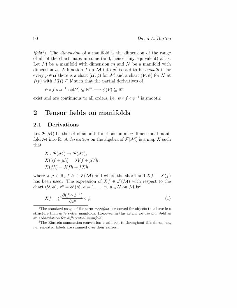
Loosely speaking, differential manifolds are generalizations of the con-cept of Euclidean spaces. Any point in a differential manifold hasan open neighbourhood that can be smoothly mapped onto an opensubset of a Euclidean space. Unlike Euclidean spaces, arbitrary dif-ferential manifolds require more than one open set to cover them.Let M be a set. A pair (U , φ), where U ⊆ M and φ : U → Rn

is a one-to-one map onto an open set φ(U) ⊆ Rn, is called a charton M. Two charts (U , φ) and (V , ψ) are called compatible if eitherU ∩ V = ∅ or else U ∩ V 6= ∅, φ(U ∩ V) and ψ(U ∩ V) are open inRn and φ ψ−1 : ψ(U ∩ V) → φ(U ∩ V) is smooth with a smoothinverse (see figure 1). An atlas is a family of charts, any two of whichare compatible and whose domains cover M. Two atlases are calledequivalent if their union is an atlas, and a set M with an equivalenceclass of such atlases is called a differential manifold (or, simply a man-

90 David A. Burton

ifold1). The dimension of a manifold is the dimension of the rangeof all of the chart maps in some (and, hence, any equivalent) atlas.Let M be a manifold with dimension m and N be a manifold withdimension n. A function f on M into N is said to be smooth if forevery p ∈ U there is a chart (U , φ) for M and a chart (V , ψ) for N atf(p) with f(U) ⊆ V such that the partial derivatives of

ψ f φ−1 : φ(U) ⊆ Rm −→ ψ(V) ⊆ Rn

exist and are continuous to all orders, i.e. ψ f φ−1 is smooth.

2 Tensor fields on manifolds

2.1 Derivations

Let F(M) be the set of smooth functions on an n-dimensional mani-fold M into R. A derivation on the algebra of F(M) is a map X suchthat

X : F(M) → F(M),

X(λf + µh) = λV f + µV h,

X(fh) = Xfh + fXh,

where λ, µ ∈ R, f, h ∈ F(M) and where the shorthand Xf ≡ X(f)has been used. The expression of Xf ∈ F(M) with respect to thechart (U , φ), xa = φa(p), a = 1, . . . , n, p ∈ U on M is2

Xf = ξa ∂(f φ−1)

∂xa φ (1)

1The standard usage of the term manifold is reserved for objects that have lessstructure than differential manifolds. However, in this article we use manifold asan abbreviation for differential manifold.

2The Einstein summation convention is adhered to throughout this document,i.e. repeated labels are summed over their ranges.


Figure 1: Loosely speaking, a differential manifold M is a collectionof points whose open neighbourhoods can be smoothly mapped ontoopen subsets of a Euclidean space. All of the maps shown in this figureare smooth with smooth inverses. The dimension of M is n.

92 David A. Burton

where ξa, ξa : U → Rn, are known as the components of X withrespect to (U , φ). Similarly, with respect to another chart (V , ψ),x′a = ψa(p), p ∈ V

Xf = ξ′a∂(f ψ−1)

∂x′a ψ (2)

on U∩V . The components ξa and ξ′a of X are related by applyingthe chain rule to (2). It can be shown that

Xf = ξ′aΦUVba

∂(f φ−1)

∂xb φ. (3)

where the transition function ΦUV is

ΦUV : U ∩ V → Rn, (4)

ΦUVab =

∂(φ ψ−1)a

∂x′b ψ (5)

where for p ∈ U ∩ V with xa = φa(p), x′a = ψa(p),

xa = (φ ψ−1)a(x′1, . . . x′n).

Comparing (3) and (1) we note that

ξa = ΦUVabξ′b

or, equivalently,

ξ′a = ΦVUabξ

b. (6)

since

ΦUVabΦVU

bc = δa

c .


2.2 Vector fields

Each point p ∈ M is equipped with an n-dimensional vector spaceTpM, called the tangent space at p. Elements of TpM are called tan-gent vectors at p. The tangent spaces are collected together to form a2n-dimensional manifold TM,

TM =⋃

p∈MTpM,

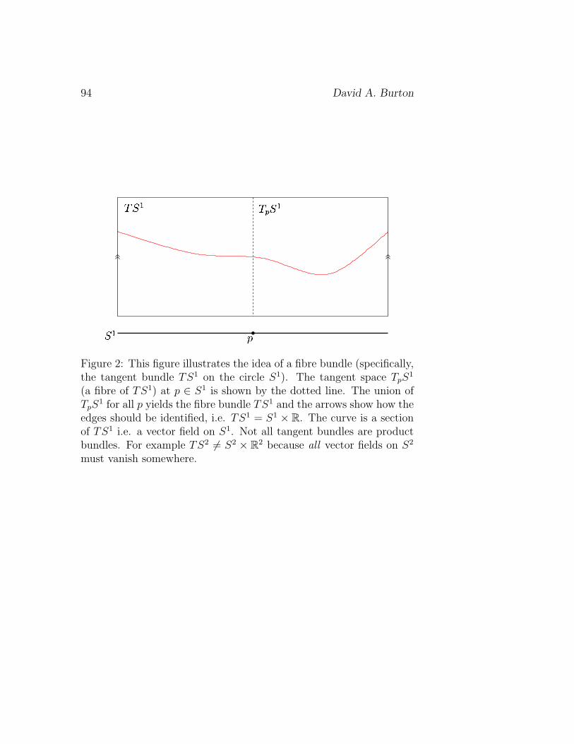
known as the tangent bundle of M, which is an example of a fibrebundle [9]. Crudely speaking, a section of a fibre bundle, such asTM, is an assignment of a point (in this case a tangent vector at p)in each fibre (in this case TpM) to its base point in the base manifold(in this case p ∈M) that varies smoothly over the base manifold (seefigure 2). Elements of the space of sections of TM, denoted ΓTM,are called vector fields. Expressed with respect to the chart (U , φ),xa = φa(p), p ∈ U a vector field X ∈ ΓTM is written

X = ξa ∂

∂xa(7)

where ξa : U → Rn are the components of X with respect to (U , φ).At each point p ∈ U the set ∂/∂xa is a vector basis for TpM. Thisnotation reflects the fact that the derivations on the algebra of F(M)and the vector fields on M are in one-to-one correspondence. Withrespect to (V , ψ), x′a = ψa(p), p ∈ V

X = ξ′a∂

∂x′a(8)

and so applying (6) to (7) and (8) we obtain

∂

∂x′a= ΦUV

ba

∂

∂xb. (9)

on U ∩ V .

94 David A. Burton

Figure 2: This figure illustrates the idea of a fibre bundle (specifically,the tangent bundle TS1 on the circle S1). The tangent space TpS

1

(a fibre of TS1) at p ∈ S1 is shown by the dotted line. The union ofTpS

1 for all p yields the fibre bundle TS1 and the arrows show how theedges should be identified, i.e. TS1 = S1 × R. The curve is a sectionof TS1 i.e. a vector field on S1. Not all tangent bundles are productbundles. For example TS2 6= S2 × R2 because all vector fields on S2

must vanish somewhere.


2.3 Differential 1-forms

A 1-form αp at p is a linear map from TpM to R, i.e. αp is an elementof the dual space T ∗

pM. The space T ∗M

T ∗M =⋃

p∈MT ∗

pM

is known as the cotangent bundle of M. Differential 1-forms are ele-ments of the space of sections of T ∗M, denoted ΓT ∗M, and they arelinear maps on vector fields into F(M). Thus,

α(X) ∈ F(M), (10)

α(fX) ≡ fα(X), (11)

α(X + Y ) ≡ α(X) + α(Y ), (12)

(α + β)(X) ≡ α(X) + β(X), (13)

where f ∈ F(M), X ∈ ΓTM, Y ∈ ΓTM, α ∈ ΓT ∗M and β ∈ΓT ∗M. We can consider vector fields as linear maps on differential1-forms by defining

X(α) ≡ α(X)

thus identifying T ∗∗M with TM. The expressions for α with respectto the charts (U , φ) and (V , ψ) used earlier are

α = αadxa

= α′adx′a.(14)

where dx′a and dxa are bases for ΓT ∗M valid on V and U respec-tively. The bases ∂/∂xa and dxa are dual,

dxa(∂/∂xb) ≡ δab ,

96 David A. Burton

as are ∂/∂x′a and dx′a,dx′a(∂/∂x′b) ≡ δa

b (15)

where δab = 1 if a = b and δa

b = 0 if a 6= b (δab is the Kronecker delta).

The contraction α(X) is chart-independent so using (15) and (6)

α(X) = α′aξ′bdx′a(

∂

∂x′b)

= α′aξ′a

= α′aΦVUabξ

b.

= αaξa

(16)

where the last line is expressed with respect to (U , φ) and so

α′a = ΦUVbaαb. (17)

Thus, using (14), the differential 1-form bases are related by

dx′a = ΦVUabdxb. (18)

on U ∩ V .

2.4 Tensor fields of arbitrary degree

Elements of the vector spaces ΓTM and ΓT ∗M are used to constructmultilinear mappings into F(M). The space Ts

rpM at p ∈M consistsof all multilinear mappings on the product of the rth-order product ofTpM and the sth-order product of T ∗

pM. Since T ∗pM is the space of

linear maps on TpM and T ∗∗p M = TpM is the space of linear maps

on T ∗pM we see that

TsrpM = (T ∗

pM× T ∗pM× . . . T ∗

pM)︸︷︷︸r times

× (TpM× TpM× . . . TpM)︸︷︷︸s times

.


A smooth type (r, s) tensor field T is an element of the space of sectionsof the type (r, s) tensor bundle

TsrM =

⋃p∈M

TsrpM,

i.e. T ∈ ΓTsrM. The integer r is called the covariant degree of

T whilst s is its contravariant degree. Special examples of tensorbundles are the tangent bundle TM = T1

0M and the cotangent bundleT ∗M = T0

1M.The tensor product ⊗ has the properties

(α⊗ T )(X,Y1, . . . Yr, α1, . . . , αs) ≡ α(X)T (Y1, . . . Yr, α1, . . . , αs),

(α⊗ β)(X, Y ) ≡ α(X)β(Y )

with

X(α) ≡ α(X)

where X, Y, Y1, . . . , Yr ∈ ΓTM and α, α1, . . . , αs, β ∈ ΓT ∗M. Thelinearity properties of the tensor product are induced from (11), (12)and (13). For example

(α⊗ β)(fX, Y ) = fα(X)β(Y )

= (α⊗ β)(X, fY )

= (fα⊗ β)(X, Y )

= (α⊗ fβ)(X, Y )

where f ∈ F(M). With respect to the chart (U , φ) the tensor T is

T = T b1...bsa1...ar

dxa1 ⊗ dxa2 ⊗ . . .⊗ dxar ⊗ ∂

∂xb1⊗ ∂

∂xb2⊗ . . .⊗ ∂

∂xbs.

98 David A. Burton

2.4.1 Metric tensor field

A metric tensor onM is a type (2, 0) symmetric non-degenerate tensorfield g ∈ ΓT0

2M. An orthonormal co-frame ea is a set of n = dimMlinearly independent sections of T ∗M with respect to which the metrichas the form

g = ηabea ⊗ eb.

where ηab = ±1 if a = b and ηab = 0 if a 6= b. If ηab = +1 whena = b then M is said to be Riemannian. Otherwise M is calledsemi-Riemannian or, alternatively, pseudo-Riemannian. A Lorentzianmanifold M is semi-Riemannian with ηab = diag(−1, 1, . . . , 1).3 Themetric tensor possesses an inverse g−1 which is the type (0, 2) tensorfield

g−1 = ηabXa ⊗Xb

where Xa is dual to ea, i.e.

ea(Xb) = δab ,

and where

ηabηbc = δac .

The frame Xa (as well as the co-frame ea) is said to be orthonor-mal.The metric establishes an isomorphism between TM and T ∗M. Givenany X ∈ ΓTM we can construct the differential 1-form g(X,−) ≡g(X,Xa)e

a. Conversely, given any differential 1-form α we have the

3For example, ηab = diag(−1, 1, 1, 1) if M is a spacetime.


vector field g−1(α,−) ≡ g−1(α, ea)Xa. For convenience we use thenotation

X ≡ g(X,−), (19)

α ≡ g−1(α,−). (20)

Thus ˜X = X and ˜α = α.

2.5 Differential forms of arbitrary degree

The totally antisymmetric type (r, 0) tensor fields on M are sectionsof the rth exterior bundle ΛrM⊂ T0

rM and are known as differentialforms of degree r or differential r-forms. The bundle of differential0-forms Λ0M is defined so that ΓΛ0M = F(M) i.e. differential 0-forms are scalar functions on M. Note that if M is an n-dimensionalmanifold then a differential r-form, with respect to an arbitrary chart,has n!/(r!(n − r)!) components. In other words, the vector spaceof differential r-forms on an n-dimensional manifold has dimensionn!/(r!(n−r)!). Let α be a differential r-form and β be a differential s-form. The exterior product of α and β, denoted α∧β, is the differential(r + s)-form given by

α ∧ β ≡ Alt(α⊗ β)

where Alt(T ) is the totally antisymmetric part of the type (r, 0) tensorT . For example, if α and β are both differential 1-forms

α ∧ β =1

2(α⊗ β − β ⊗ α).

It can be shown that for α ∈ ΓΛrM and β ∈ ΓΛsM

α ∧ β = (−1)rsβ ∧ α

100 David A. Burton

and that the exterior product is associative

α ∧ (β ∧ γ) = (α ∧ β) ∧ γ

≡ α ∧ β ∧ γ.

where γ ∈ ΓΛtM. Conventionally, the exterior product symbol isdropped when applied to a differential 0-form f and a differential r-form α, i.e. fα ≡ f ∧ α = α ∧ f .All differential r-forms are special examples of sections of the exteriorbundle ΛM. A general section of ΛM consists of linear combina-tions of differential forms of different degrees. Such differential formsare termed inhomogenous, whilst differential r-forms are called ho-mogenous. The vector space of inhomogenous differential forms on ann-dimensional manifold has dimension 2n.

2.6 Example

Let V be a vector field and α be a differential 1-form on the 2-dimensional manifold M = R2. Let (x, y) = φ(p) be the componentsof a Cartesian chart (U , φ) at p ∈ U = R2. This means that the metrictensor has the form

g = dx⊗ dx + dy ⊗ dy

over U . If (r, θ) = ψ(p) are the components of the polar chart (V , ψ)at p ∈ V = R2 − 0 given by

(x, y) = (r cos θ, r sin θ)

and since

(x, y) = φ(p)

= φ ψ−1 ψ(p)

= φ ψ−1(r, θ)


we see that

φ ψ−1(r, θ) = (r cos θ, r sin θ).

Thus, using (17) and (5) we find that

dx = cos θdr − r sin θdθ,

dy = sin θdr + r cos θdθ

and so

g = dr ⊗ dr + r2dθ ⊗ dθ.

Note that ∂/∂r, (1/r)∂/∂θ and dr, rdθ are a dual orthonormalframe and co-frame valid over V .An inhomogenous form Φ on M expressed with respect to (U , φ) hasthe structure

Φ = a(x, y) + b(x, y)dx + c(x, y)dy + f(x, y)dx ∧ dy.

3 The tools of exterior calculus

Let α be a differential 1-form, β be a differential p-form, γ be anarbitrary degree differential form, f be a scalar field and X be a vectorfield on an n-dimensional manifold M. The exterior derivative d ondifferential forms is defined by the properties

df(X) = Xf, (21)

d(β ∧ γ) = dβ ∧ γ + (−1)pβ ∧ dγ, (22)

ddγ = 0. (23)

With respect to the chart (U , φ)

X = ξa ∂

∂xa

102 David A. Burton

and so, referring to (1)

Xf = ξa ∂

∂xa(f φ−1) φ.

However,

df(X) = ξadf(∂

∂xa)

and so, since X is arbitrary, the exterior derivative on 0-forms has thelocal form

df =

[∂

∂xa(f φ−1) φ

]dxa.

The interior operator ιX with respect to the vector field X is definedby

ιXα = α(X), (24)

ιX(β ∧ γ) = ιXβ ∧ γ + (−1)pβ ∧ ιXγ, (25)

ιXιXγ = 0. (26)

Both d and ιX are extended to inhomogenous differential forms bylinearity. Specifically, if

α =n∑

q=0

αq

where αq ∈ ΓΛqM then

dα =n∑

q=0

dαq,

ιXα =n∑

q=0

ιXαq.


The dimension of the vector space of differential p-forms is n!/(p!(n−p)!). Thus, the vector spaces of differential p-forms and (n− p)-formshave the same dimension. The Hodge map ? is a linear isomorphismbetween the vector spaces of differential p- and (n−p)-forms satisfying

?(γ ∧ X) = ιX ? γ, (27)

?(fγ) = f ? γ (28)

and is completely defined by specifying an orientation, or volume form,denoted ?1 ∈ ΓΛnM. The orientation is specified through the metrictensor g on M and has the form

?1 = ±e1 ∧ e2 ∧ · · · ∧ en

where ea is any orthonormal co-frame (see subsection 2.4.1). Thechoice of sign is a matter of taste, and on R3 can be identified withthe choice of left- or right-handedness of orthonormal frames. Using(28) and (27) a repeated application of the Hodge map on a p-form βcan be shown to yield

? ? β = det(η)(−1)p(n−p)β (29)

where η is the matrix of components ηab = g(Xa, Xb) of the metric gwith respect to an orthonormal frame Xa and β ∈ ΓΛpM. Thus,

the inverse Hodge map−1? is

−1? β = det(η)(−1)p(n−p) ? β.

A useful identity involving the interior operator and Hodge map isthat

X ∧ ?β = −(−1)p ? ιXβ (30)

104 David A. Burton

where, again, β ∈ ΓΛpM. Therefore, the metric contraction of twodifferential 1-forms α and β on M can be expressed in the form

g−1(α, β) =−1?

(α ∧ ?β

).

Indeed, the Hodge map is used to define an inner product on homoge-nous differential forms on Riemannian manifolds and an indefiniteinner product on semi-Riemannian manifolds :

α · β ≡ −1?

(α ∧ ?β

)

where α and β are homogenous differential forms with the same degree.A differential form α that satisfies

dα = 0

is said to be closed. If a differential form β can be written

β = dγ (31)

where γ is another differential form then β is called exact. A beautiful,and very powerful, lemma due to Poincare is that any closed differ-ential form can be written locally as an exact differential form. Moreprecisely, if dα = 0 on M then for any p ∈ M there exists an openneighbourhood of p on which α = dβ. That this cannot, in general,be done globally is a consequence of the topology of M.

3.1 Example

Let α be a 1-form on a 2-dimensional differential manifold (M, g).With respect to a chart (U , φ) α has the form

α = a(x, y)dx + b(x, y)dy


Note that

dα = da ∧ dx + ad(dx) + db ∧ dy + bd(dy),

= da ∧ dx + db ∧ dy

using (22) and (23). Since dx, dy is dual to ∂/∂x, ∂/∂y we notethat

da = da(∂/∂x)dx + da(∂/∂y)dy

and so, by (21)

da =∂a

∂xdx +

∂a

∂ydy.

Using the symmetry properties of the exterior product

dx ∧ dx = dy ∧ dy = 0

dy ∧ dx = −dx ∧ dy

and we conclude that

dα =( ∂b

∂x− ∂a

∂y

)dx ∧ dy.

With respect to (U , φ) the volume form ?1 will be

?1 = hdx ∧ dy

where h is the component of ?1 with respect to (U , φ). The Hodgedual of α is

?α = ια ? 1

= ια(hdx ∧ dy)

= hιαdx ∧ dy − hdx ∧ ιαdy

= hg−1(α, dx)dy − hg−1(α, dy)dx

using (20), (27), (25) and (24).

106 David A. Burton

4 Integration of forms over chains

4.1 The pull-back of differential forms

A smooth map f : M → N induces the pull-back map f ∗ : ΛN →ΛM that takes differential forms on N to differential forms on M.Let (U , φ) be a chart on M with components xa = φa(p) at p ∈ Mand let (V , ψ) be a chart on N with components yµ = ψµ(q) at q ∈ N .The pull-back f ∗h of the 0-form h ∈ ΓΛ0N = F(M) with respect tof is

f ∗h ≡ h f.

The pull-back f ∗α of α ∈ ΓΛ1N , where

α = αµdyµ

with respect to (V , ψ), is the differential 1-form on M given by

f ∗α = αµ f∂

∂xa(ψµ f φ−1) φdxa

when expressed with respect to (U , φ). The pull-back operation isextended to higher degree differential forms as a tensor homomorphism

f ∗(α ∧ β

)= f ∗α ∧ f ∗β (32)

where β is a differential form. It can be shown that the exteriorderivative and pull-back operations commute

f ∗dα = df ∗α. (33)


4.2 Cubes and chains

Let (U , φ), [0, 1]r ⊂ U , be the natural chart on Rr, i.e. σj = φj(p), and0 ≤ σj ≤ 1,j ∈ Z. An r-cube4 on a differential manifold M is the pair(cr, Ωr) where cr : [0, 1]r →M is a smooth map and

Ωr = ±dσj1 ∧ dσj2 ∧ . . . dσjr , j1, j2, . . . jr ∈ Z, (34)

is a differential r-form (an orientation) on Rr. We will examine thechoice of sign shortly.A finite sum of r-cubes (cr

J , ΩrJ) with real coefficients bJ, J ∈ Z,

is called an r-chain.Each r-cube gives rise to 2r (r − 1)-cubes known as faces. Each face,denoted cr−1

j,ε , is obtained by restricting cr to the points p ∈ [0, 1]r such

that σj = φj(p) = ε, where ε = 0, 1. The orientation Ωr−1j,ε of each face

is obtained from Ωr by

Ωr−1j,ε ≡ (−1)ε+1ι∂/∂σjΩr. (35)

Note that faces inherit their orientation from that of a higher-dimensionalcube, which we call their parent cube. Once a parent cube is definedall of the orientations of its faces are fixed by (35). Thus, the sign in(34) must either be fixed as part of the definition of Ωr if (cr, Ωr) is aparent cube, or inherited from its parent cube through (35).The r-cube (cr, Ωr) has a boundary (r − 1)-chain ∂(cr, Ωr),

∂(cr, Ωr) =r∑

j=1

∑ε=0,1

(cr−1j,ε , Ωr−1

j,ε ),

where the (r−1)-cube in each term of the summand is a face of (cr, Ωr).The boundary ∂Cr of the r-chain Cr

Cr =∑

J

bJ(crJ , Ωr

J) (36)

4Technically, this is an oriented r-cube.

108 David A. Burton

is

∂Cr ≡∑

J

bJ∂(crJ , Ωr

J).

4.2.1 Example

Let (c2, Ω2) be a 2-cube on a 2-dimensional manifold M. We canalways find a chart (U , φ) on M with respect to which the componentsof c2 are the identity map. The chart (U , φ) is said to be adapted toc2. Thus, with x = φ1(p) and y = φ2(p) at p ∈ U , the map c2 hascomponents

(x, y) = c2(σ1, σ2) = (σ1, σ2).

The orientation associated with c2 is

Ω2 = dσ1 ∧ dσ2.

The faces of the parent cube (c2, Ω2) are

(x, y) = c11,0(0, σ

2) = (0, σ2),

(x, y) = c11,1(1, σ

2) = (1, σ2),

(x, y) = c12,0(σ

1, 0) = (σ1, 0),

(x, y) = c12,0(σ

1, 1) = (σ1, 1)

with orientations

Ω11,0 = −dσ2

Ω11,1 = dσ2

Ω12,0 = dσ1

Ω12,1 = −dσ1.


Thus, the 1-chain ∂(c2, Ω2) is

∂(c2, Ω2) =(c11,0,−dσ2) + (c1

1,1, dσ2)

+ (c12,0, dσ1) + (c1

2,1,−dσ1).

4.3 Integration and Stokes’ theorem

Any differential r-form ω on Rr can be written

ω = fΩr

where f is a smooth function on Rr and

Ωr = ±dσj1 ∧ dσj2 ∧ . . . dσjr .

The integral of ω over [0, 1]r is defined to be

∫

[0,1]rω =

∫

[0,1]rf(σj1 , σj2 , . . . σjr)Ωr

≡1∫

0

1∫

0

. . .

1∫

0

f(σj1 , σj2 , . . . σjr)dσj1dσj2 . . . dσjr

(37)

regardless of the choice of sign in Ωr. The integral of a differentialr-form α on any manifold M over the r-cube (cr, Ωr) is defined viathe pull-back map cr∗. The r-form cr∗α on Rr is, with respect to thechart (U , φ), σ = φj(p) at p ∈ Rr,

cr∗α = hΩr

where h is a smooth function on Rr. We define∫

cr

α ≡∫

[0,1]rcr∗α

110 David A. Burton

and so using (37)

∫

[0,1]rcr∗α =

∫

[0,1]rh(σj1 , σj2 , . . . σjr)Ωr

=

∫

[0,1]rh(σj1 , σj2 , . . . σjr)dσj1dσj2 . . . dσjr .

The integral of α over

Cr =∑

J

bJ(crJ , Ωr

J)

is∫

Cr

α ≡∑

J

bJ

∫

crJ

α.

This formalism leads to the remarkably beautiful result known as theNewton-Leibniz-Gauss-Green-Ostrogradskii-Stokes-Poincare theorem,or Stokes’ theorem for short,

∫

Cr

dα =

∫

∂Cr

α. (38)

Thus, using (22) we have an analogue of the “integration by parts”formula,

∫

Cr

dα ∧ β =

∫

∂Cr

α ∧ β − (−1)p

∫

Cr

α ∧ dβ

where α is a differential p-form. For notational simplicity, although itis an abuse of the notation, if an r-chain consists of only one r-cubethen we shall use the same label for the r-cube map as used for ther-chain.


4.4 Example

Let (U , φ) be a spherical polar chart on M = R3, i.e. one in whichthe metric has the form

g = dr ⊗ dr + r2(dθ ⊗ dθ + sin2 θdϕ⊗ dϕ).

Thus,

e1 = dr

e2 = rdθ

e3 = r sin θdϕ

is an orthonormal co-frame. Let us choose the orientation

?1 = e1 ∧ e2 ∧ e3

= r2 sin θdr ∧ dθ ∧ dϕ.

Let Σ be a 2-chain on R3 consisting of only one 2-cube with

r = 1

θ = Σ1(p) = πσ1,

ϕ = Σ2(p) = 2πσ2

and orientation Ω2 = dσ1 ∧ dσ2. The pull-back with respect to Σ ofeach element of the cobasis dr, dθ, dφ is

Σ∗dr = dΣ∗r = d1 = 0,

Σ∗dθ = dΣ∗θ = πdσ1,

Σ∗dφ = dΣ∗φ = 2πdσ2

using (33). The vector field ∂/∂r is normal to the image set DΣ of Σ,i.e.

Σ∗(g(∂/∂r,−))

= Σ∗dr

= 0

112 David A. Burton

A volume form on DΣ induced from ?1 is

#1 = ι∂/∂r ? 1

and so the area of DΣ is

∫

Σ

#1 =

∫

[0,1]2Σ∗#1

=

∫

[0,1]2Σ∗(sin θdθ ∧ dϕ)

= 2π2

∫

[0,1]2sin(πσ1)dσ1 ∧ dσ2

= 2π2

∫

[0,1]2sin(πσ1)Ω2

= 2π2

1∫

0

1∫

0

sin(πσ1)dσ1dσ2

= 4π.

Note that the “outward” pointing normal (i.e. that which points awayfrom the coordinate singularity at r = 0) was used to construct #1.An alternative (although less conventional) choice is to use the “in-ward” pointing normal −∂/∂r.

5 Standard vector calculus in terms of

exterior calculus

Let us focus on the special case M = R3 endowed with the standardEuclidean metric. This means there exists a global chart (R3, φ), where


xa = φa(p), p ∈ R3, with respect to which the metric tensor g hasthe form

g = dx1 ⊗ dx1 + dx2 ⊗ dx2 + dx3 ⊗ dx3.

Such charts on R3 are called Cartesian. We choose the orientation

?1 = dx1 ∧ dx2 ∧ dx3

and note that, using (29),

?2α = α (39)

for any degree differential form α on R3. Thus

−1? α = ?α. (40)

To see this observe that ∂/∂x, ∂/∂y, ∂/∂z is an orthonormal frameand that, in the notation of (29), det η = 1. Furthermore, the valuesof p(3− p) for each p ∈ 0, 1, 2, 3 are all even.Let i, j,k be the unit orthonormal vector basis, in the conventionalsense, corresponding to ∂/∂x, ∂/∂y, ∂/∂z. This means that givena conventional vector field u we construct a vector field U on R3

considered as a manifold by the following replacements :

i → ∂/∂x,

j → ∂/∂y,

k → ∂/∂z.

Thus, if

u = a(x, y, z)i + b(x, y, z)j + c(x, y, z)k

then U , with respect to the chart (R3, φ), has the form

U = a(x, y, z)∂

∂x+ b(x, y, z)

∂

∂y+ c(x, y, z)

∂

∂z.

We will indicate this correspondence as equality, i.e.

U = u.

114 David A. Burton

5.1 Dot and cross products

Let u and v be conventional vector fields on R3 and their correspond-ing vector fields on R3, considered as a manifold, be U = u and V = v.Then, the conventional dot product u · v is

u · v = g(U, V )

whilst the conventional cross product u× v is

u× v = g−1(?(U ∧ V ),−).

The cyclic symmetry of the triple vector product

u · (v ×w) = v · (w × u) = w · (u× v)

follows as a consequence of the properties of the exterior product

u · (v ×w) = g−1(?(U ∧ V ∧ W ),−)

= g−1(?(V ∧ W ∧ U),−)

= g−1(?(W ∧ U ∧ V ),−)

where W = w.

5.2 Grad, curl and div

The operations grad,curl and div are

grad(f) = df , (41)

curl(u) = ?dU , (42)

div(u) =−1? d ? U (43)


in exterior form, where f is a smooth function on R3. All of the well-known identities involving these three operations can be obtained in astraightforward manner using the material in section 3. For example

?d2f = 0

= curl(grad(f)),

using (23) and

div(u× v) =−1? d ?

(?(U ∧ V )

)

=−1? d(U ∧ V )

=−1?

(dU ∧ V − U ∧ dV

)

= ιV ? dU − ιU ? dV

= g(?dU , V )− g(?dV , U)

= v · curl(u)− u · curl(v)

using (43), (39), (22), (40), (27), (24) and (42).

5.3 Integral relations

Let Ω : [0, 1]3 → R3 and Σ : [0, 1]2 → R3 be an oriented 3-chain and2-chain respectively. Let their image sets be labelled DΩ and DΣ. Letthe outward pointing normal of the image set DC2 of a 2-chain C2 belabelled nC2 as a conventional vector field and NC2 as a vector fieldon R3 as a manifold. Let dµ3, dµ2

C2 be integration measures such that

∫

DΩ

fdµ3 =

∫

Ω

f ? 1, (44)

∫

DC2

fdµ2C2 =

∫

C2

f ? NC2 (45)

116 David A. Burton

where f is any smooth function. The traditional Stokes’ theorem∫

DΣ

curl(v) · nΣdµ2Σ =

∫

D∂Σ

v · dr (46)

and divergence theorem∫

DΩ

div(v)dµ3 =

∫

D∂Ω

v · n∂Ωdµ2∂Ω, (47)

are consequences of (38) with Cr = Σ and Cr = Ω respectively.Let us first focus on (47). We note that

∫

DΩ

div(u)dµ3 =

∫

Ω

(−1? d ? U) ? 1

=

∫

Ω

?(−1? d ? U)

=

∫

Ω

d ? U

=

∫

∂Ω

?U .

(48)

To go further we need to examine the integrand in (48). Any differ-ential 1-form α on R3 can be written in the form

α = α(NC2)NC2 + β

ιNC2β = 0

and since

ιNC2β ? 1 = NC2 ∧ ?β

using (30) we note that

NC2 ∧ ?β = 0


implying that

?β = NC2 ∧ γ

where γ is a differential 1-form. Since

C2∗NC2 = C2∗[NC2(Xα)eα] = 0

where Xα, NC2, α = 1, 2, is a frame adapted to C2 with dual co-frame eα, NC2, it follows that using (32)

C2∗ ? β = 0.

Therefore,

C2∗ ? α = C2∗[α(NC2) ? NC2

]. (49)

Continuing with (48) we find that

∫

DΩ

div(u)dµ3 =

∫

∂Ω

?U

=

∫

∂Ω

g(U,N∂Ω) ? NC2

=

∫

D∂Ω

u · ndµ2∂Ω

(50)

which is the conventional divergence theorem. Equation (49) is usedin the penultimate step.

118 David A. Burton

Similarly, focussing on (46) we obtain the conventional Stokes’ theorem

∫

DΣ

curl(v) · nΣdµ2Σ =

∫

Σ

(ιNΣ

−1? dV

)? NΣ

=

∫

Σ

?(NΣιNΣ

−1? dV

)

=

∫

Σ

?(−1

? dV)

=

∫

Σ

dV

=

∫

∂Σ

V

=

∫

[0,1]

(∂Σ)∗V

=

∫ 1

0

Va ∂Σ(σ)d∂Σa

dσ(σ)dσ

=

∫ 1

0

v(σ) · dr

dσ(σ)dσ

=

∫

D∂Σ

v · dr

(51)

where Va = V (∂/∂xa) and r(σ) is the position vector that locates thepoint labelled by σ on D∂Σ, i.e.

r(σ) = ∂Σa(σ)∂

∂xa.

5.4 Applications involving Stokes’ theorem on R3

Note the plethora of metric and Hodge operations that occur whencomparing conventional vectorial equations with their equivalent dif-


ferential form equations. The reason is that we have insisted on re-placing conventional vector field, for example u, with their differentialgeometric vector field counterparts, for example U . However, thisis often not the best strategy to adopt. The formalism is at its mostpowerful when it is recognized that many vectorial quantities are moreefficiently represented by differential forms. For example, if V is thevelocity of a fluid flow on R3 then it is natural to work with the vor-ticity 2-form ω

ω = dV

rather than the vector field W

W = ?dV .

The vorticity Γ[Σ] across a 2-chain Σ is simply

Γ[Σ] ≡∫

Σ

ω

=

∫

Σ

dV

=

∫

∂Σ

V

which shows that the vorticity is just the circulation around the 1-chain ∂Σ.Another nice example is to consider the electric field of an isolatedstatic point charge. Traditionally, one thinks in terms of an electricfield vector E and an electric potential Φ where E = −grad(Φ). Here,it is more natural to think in terms of an electric differential 1-formE = −dΦ (where E = E) on the 3-dimensional differential manifold(M, g), M = R3 − p where p is the location of the point source.That E is divergence-free means that

d ? E = 0 (52)

120 David A. Burton

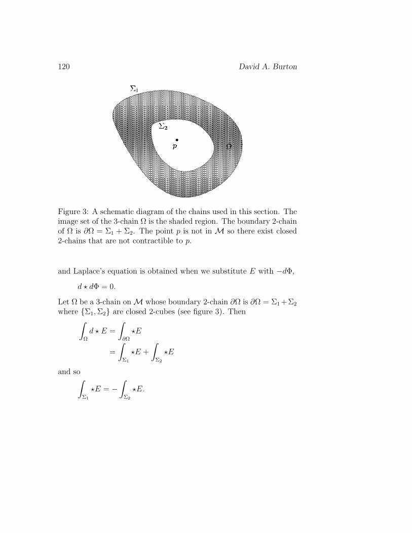
Figure 3: A schematic diagram of the chains used in this section. Theimage set of the 3-chain Ω is the shaded region. The boundary 2-chainof Ω is ∂Ω = Σ1 + Σ2. The point p is not in M so there exist closed2-chains that are not contractible to p.

and Laplace’s equation is obtained when we substitute E with −dΦ,

d ? dΦ = 0.

Let Ω be a 3-chain on M whose boundary 2-chain ∂Ω is ∂Ω = Σ1 +Σ2

where Σ1, Σ2 are closed 2-cubes (see figure 3). Then∫

Ω

d ? E =

∫

∂Ω

?E

=

∫

Σ1

?E +

∫

Σ2

?E

and so∫

Σ1

?E = −∫

Σ2

?E.


Since the normals to the images of the 2-chains Σ1 and Σ2 are oppo-sitely oriented we conclude that

P [Σ] ≡∫

Σ

?E,

is the same for all Σ topologically equivalent to Σ1. The Poincarelemma tells us that that ?E = dα on an open subset U ⊂M where αis a differential 1-form on U . However ?E is not exact, i.e. cannot bewritten dα where α is a differential form on all of M and so P [Σ] isin general non-zero.The number P [Σ] is known as the de Rham period of ?E over Σ and,physically, it is the electric charge of the point p. In a spherical polarchart (U , ψ) with p located at r = 0 the metric tensor has the form

g = dr ⊗ dr + r2dθ ⊗ dθ + r2 sin2 θ.dϕ⊗ dϕ,

A solution to Laplace’s equation on M is

Φ(r, θ, ϕ) =c

r

where c is a constant scalar. To see this, choose the orientation

?1 = +e1 ∧ e2 ∧ e3

where e1, e2, e3 is the orthonormal co-frame

e1 = dr,

e2 = rdθ,

e3 = r sin θdϕ.

122 David A. Burton

Thus,

?dΦ = ?dc

r,

= − ?c

r2dr,

= − c

r2? e1,

= − c

r2e2 ∧ e3,

= −c sin θdθ ∧ dϕ

and so, as promised, d ? dΦ = 0 on M. The de Rham period of ?dΦover the 2-chain (Σ, dσ1∧dσ2) with components r = r0, θ = πσ1, ϕ =2πσ2 is

∫

Σ

?dΦ =

∫

Σ

−c sin θdθ ∧ dϕ

= −4πc.

Introducing the charge q ≡ −4πc of the source we see that

Φ(r, θ, ϕ) = − q

4πr

which is the electric potential of an electric monopole of charge q atp.

6 Differential operators on tensor bun-

dles

So far the only differential operator that we have discussed is theexterior derivative d on the bundle of differential forms. It is also veryuseful to be able to differentiate arbitrary type tensors, which is the


focus of this section. We will discuss two types of differential operatorson tensors bundles : the Lie derivative and linear connections. Sofar we have only considered vector fields in terms of derivations onF(M). Before we can discuss the Lie derivative we need to introducethe notion of the flow of a vector field.

6.1 The push-forward map

Recall that a smooth map f : M→N between two manifolds M andN induces the pull-back map f ∗ : ΛN → ΛM (see section 4.1). If f isone-to-one then it also induces the push-forward map f∗ : TM→ TNbetween the tangent bundles of M and N . Let X ∈ ΓTM be avector field on M and define the push-forward of X with respect tof , denoted by f∗X, via

f ∗[α(f∗X)] = (f ∗α)(X)

where α ∈ ΓΛ1N is any differential 1-form on N . In particular if wechoose α = dh we find

f ∗[dh(f∗X)] = (f ∗dh)(X)

= d(f ∗h)(X)

= X(f ∗h)

but, on the other hand,

f ∗[dh(f∗X)] = f ∗[(f∗X)(h)]

and so we obtain the action of f∗X on any h ∈ F(N ) :

f ∗[(f∗X)(h)] = X(f ∗h).

124 David A. Burton

6.2 One-parameter families of diffeomorphisms

Let M be a differential manifold, V ⊂ M be an open subset of Mand I ⊂ R be an open interval about 0 ∈ R. Let ϕ be a map suchthat

ϕ :I × V →M(t, p) → q = ϕ(t, p) ≡ ϕt(p)

where, for each t ∈ I, ϕt is a local diffeomorphism (a smooth map withsmooth inverse) of V to another open subset of M. We demand thatfor any pair t1, t2 ∈ I such that (t1 + t2) ∈ I

ϕt2 ϕt1 = ϕt1+t2

and

ϕ0(p) = p ∀ p ∈M.

Note that in particular ϕ−1t = ϕ−t. The collection of maps ϕt is

known as a one-parameter family of local diffeomorphisms and inducesa curve (a 1-chain) Cp for each p ∈M

Cp : I →Mt → ϕt(p).

The push-forward Cp∗∂t (where ∂t ≡ ∂/∂t) when evaluated at t = 0yields a tangent vector Xp ∈ TpM at p

Xp = Cp∗∂t|t=0.

Since ϕt is smooth the set Xp leads to the vector field X ∈ ΓTMgiven by

X|p ≡ Xp


and so a one-parameter family of local diffeomorphisms on M inducesa vector field on M. Conversely, given a vector field X ∈ ΓTM onecan generate a one-parameter family ψt of local diffeomorphisms ofM by solving for a set of integral curves Cp of X (also known as theflow of X)

Cp : I →Mt → q = Cp(t)

Cp∗∂t = X

Cp(0) = p

and then defining

ψt(p) ≡ Cp(t).

With respect to a local chart (U , φ), with coordinates xa, the abovebecomes

C∗p [dxa(Cp∗∂t)] = dCap/dt

= C∗p [dxa(X)]

= ξa Cp

where ξa and Cap are the components of X and Cp with respect

to (U , φ). Equations Cp∗∂t = X and Cp(0) = p translated into adifferential equation for ψ read

dψa

dt(t, p) = (ξa ψ)(t, p)

subject to the initial condition

ψa(0, p) = xa0

where xa0 = φa(p) is the coordinate representation of p ∈ M with

respect (U , φ).

126 David A. Burton

6.2.1 Example

Let X ∈ ΓTM, dimM = 2, be the vector field

X = y∂

∂x− x

∂

∂y

with respect to a chart (U , φ) with coordinates x, y. An integralcurve C : [0, 1] →M of X is a solution to

C∗∂t = X

or, in componential form where x = C1(t), y = C2(t),dC1

dt= C2(t),

dC2

dt= −C1(t)

which with the initial condition

C1(0) = a,

C2(0) = b,

has the solution

C1(t) = a cos(t) + b sin(t),

C2(t) = −a sin(t) + b cos(t).

Thus X induces a one-parameter family of local diffeomorphisms ψtwhose coordinate expressions are

ψ1t (x, y) = x cos(t) + y sin(t),

ψ2t (x, y) = −x sin(t) + y cos(t).


6.3 The Lie derivative

The notion of one-parameter families of local diffeomorphisms of Mleads very naturally to a type-preserving derivation on tensor fieldsknown as the Lie derivative. Let ϕt be a one-parameter familyof local diffeomorphisms of M with p = ϕ0(p) and define the one-parameter family of maps ϕt by

ϕtα = ϕ∗t α,

ϕtX = ϕ−t∗X,

ϕt(S ⊗ T ) = ϕtS ⊗ ϕtT

where α is a differential form, X is a vector field and S and T arearbitrary type tensors on M. The Lie derivative LXT of a tensor Tat p ∈M with respect to the vector field X induced from ϕt is

LXT (p) ≡ limt→0

1

t(ϕtT − ϕ0T )(p). (53)

For example, for f ∈ ΓΛ0M (i.e. f ∈ F(M))

LXf(p) = limt→0

1

t(ϕ∗t f − ϕ∗0f)(p)

= limt→0

1

tf [ϕt(p)]− f(p)

= (Cp∗∂t)(f)|t=0

= Xf(p)

i.e.

LXf = Xf. (54)

It can also be shown that

(LXY )f(p) = X(Y f)(p)− Y (Xf)(p) (55)

128 David A. Burton

or

LXY = [X,Y ] (56)

where Y is a vector field and the commutator [X,Y ] ≡ XY − Y X isknown as the Lie bracket of X and Y . Let xa be the coordinates of achart (U , φ) onM with associated local coordinate basis ∂a = ∂/∂xafor ΓTM. Then

[X, Y ]f = X(Y f)− Y (Xf)

= ξa∂a(ζb∂bf)− ζa∂a(ξ

b∂bf)

= (ξa∂aζb − ζa∂aξ

b)∂bf

where X = ξa∂a and Y = ζa∂a and the last line is obtained because∂a∂bf = ∂b∂af . Therefore, a coordinate expression for the Lie bracketon U is

[X, Y ] = (ξa∂aζb − ζa∂aξ

b)∂b.

It can be shown that, when applied to differential forms, the Lie deriva-tive has the representation

LXα = dιXα + ιXdα (57)

where α is a differential form on M. Equation (57) is known as Car-tan’s identity. More generally, LX is a type-preserving

T ∈ ΓTpqM⇒ LXT ∈ ΓTp

qMderivation on tensor fields

LX(S ⊗ T ) = LXS ⊗ T + S ⊗ LXT, (58)

where S and T are arbitrary type tensors on M, that commutes withcontractions

LX [α(Y )] = (LXα)(Y )− α(LXY ), (59)


where α is a differential 1-form and Y is a vector field onM, commuteswith the exterior derivative d

LXd = dLX

on differential forms on M and satisfies

[LX ,LY ] ≡ LXLY − LYLX

= L[X,Y ].

It turns out that (54), (56), (58) and (59) are enough to specify LX

uniquely : the Lie derivative is the unique type-preserving derivationon tensor fields that commutes with contractions and satisfies (56).Finally, the Lie derivative also commutes with push-forwards

ψ∗(LXY ) = Lψ∗Xψ∗Y

and pull-backs

ψ∗(Lψ∗Xα) = LXψ∗α

where ψ : M → N is a smooth one-to-one map between differentialmanifolds M and N , X, Y ∈ ΓTM and α ∈ ΓΛN .

6.3.1 Example

Let x, y be the coordinates of a chart (U , φ) on a 2-dimensionaldifferential manifold M. Then

Lcos(y)∂x [sin(x)dy] = Lcos(y)∂x [sin(x)]dy + sin(x)Lcos(y)∂xdy

= cos(y)∂x[sin(x)]dy + sin(x)d(Lcos(y)∂xy)

= cos(y) cos(x)dy + sin(x)d[cos(y)∂xy]

= cos(y) cos(x)dy

130 David A. Burton

and

Lcos(y)∂x [sin(x)∂y] = Lcos(y)∂x [sin(x)]∂y + sin(x)Lcos(y)∂x∂y

= cos(y)∂x[sin(x)]∂y − sin(x)L∂y [cos(y)∂x]

= cos(y) cos(x)∂y − sin(x)L∂y [cos(y)]∂x − sin(x) cos(y)L∂y∂x

= cos(y) cos(x)∂y − sin(x)∂y[cos(y)]∂x

= cos(y) cos(x)∂y + sin(x) sin(y)∂x.

6.4 Linear connections on tensor bundles

So far we have introduced two important differential operators : theexterior derivative d that acts on differential forms and the Lie deriva-tive that acts on any tensor field. However, we do not as yet haveanything that resembles a “directional derivative” of tensors alongvector fields. For example, one often constructs the conventional vec-tor field (u · ∇)v on R3 out of two conventional vector fields u and vwhere

v = ai + bj + ck,

(u · ∇)v ≡ [u · grad(a)]i + [u · grad(b)]j + [u · grad(a)]k.

Let us define the operator D where D(u,v) ≡ (u ·∇)v and D(u, f) ≡u · grad(f) where f is a scalar on R3. Note that D(fu,v) = fD(u,v)i.e. D is linear in its first argument. Furthermore it obeys the Leibnizrule on its second argument i.e. D(u, fv) = D(u, f)v+fD(u,v). Wealready have a differential operator, the Lie derivative, that maps twovector fields on M to another vector field on M. However, althoughit obeys the Leibnitz rule

LX(fY ) = (LXf)Y + fLXY

it is not linear in its first argument since

LfXY = −LY (fX)

= −(LY f)X + fLXY.


So, in order to discuss “directional derivatives” of tensor fields ondifferential manifolds we need to introduce some new machinery.A linear connection ∇ on a differential manifold M is a map

∇ : ΓTM× ΓTM→ ΓTM(X, Y ) → ∇XY

such that

∇X(fY ) = (∇Xf)Y + f∇XY,

∇Xf = Xf,

∇fXY = f∇XY

where f ∈ F(M) and is extended to arbitrary type tensor fields bydemanding that it commutes with contractions

∇X [α(Y )] = (∇Xα)(Y ) + α(∇XY ),

where α ∈ ΓΛ1M, and is a tensor derivation

∇X(S ⊗ T ) = ∇XS ⊗ T + S ⊗∇XT

where S and T are tensors on M. Unlike the Lie derivative a linearconnection is, by definition, linear in its first argument. Furthermore,the above properties are not enough to specify ∇ uniquely. There aremany maps that satisfy the defining properties of a linear connection.

6.4.1 Example

Let (U , φ) be a chart with coordinates x, y on a 2-dimensional dif-ferential manifold M. A linear connection is fixed by giving its action

132 David A. Burton

on ∂x, ∂y, say

∇∂x∂x = x∂y,

∇∂x∂y = 0,

∇∂y∂x = y2∂x,

∇∂y∂y = sin(xy)∂y,

and inducing its action on all other vector fields and arbitrary typetensors by the fundamental properties of all linear connections. Forexample, on the co-frame dx, dy dual to ∂x, ∂y

(∇∂xdy)(∂x) = ∂x[dy(∂x)]− dy(∇∂x∂x) = −x

(∇∂xdy)(∂y) = ∂x[dy(∂y)]− dy(∇∂x∂y) = 0

so

∇∂xdy = −xdx.

Furthermore

∇∂x [cos(x)dy] = ∂x[cos(x)]dy + cos(x)∇∂xdy

= − sin(x)dy − cos(x)xdx.

6.4.2 Connection 1-forms

Every linear connection ∇ on an n-dimensional differential manifoldM has a set of n2 differential 1-forms ωa

b, known as connection1-forms, associated with each basis Xa for ΓTM. They are givenby

∇XaXb = ωcb(Xa)Xc. (60)

The fundamental properties of ∇ induce its action on the co-frameea dual to Xa :

(∇Xaeb)(Xc) = ∇Xa [e

b(Xc)]− eb(∇XaXc)

= −eb(∇XaXc)


and so

∇Xaeb = −ωb

c(Xa)ec. (61)

Connection 1-forms induced by different bases are related by

ω′ab = Λbcωe

c

−1

Λea +

−1

ΛcadΛb

c (62)

where

X ′a = Λa

bXb,

Xa =−1

ΛabX ′

b,

∇X′aX ′

b = ω′cb(X′a)X

′c.

6.4.3 Torsion

Any linear connection and the Lie derivative can be combined to formtwo important tensor fields called torsion and curvature. The torsionoperator T : ΓTM× ΓTM→ ΓTM induced by a linear connection∇ on M is

TX,Y ≡ ∇XY −∇Y X − [X,Y ], (63)

where X,Y ∈ ΓTM. Since T can be shown to be linear in all argu-ments,

TX+Y,Z = TX,Z + TY,Z ,

TX,Y +Z = TX,Y + TX,Z ,

TfX,Y = TX,fY = fTX,Y ,

where f ∈ F(M) and Z ∈ ΓTM, there must exist a type (2, 1) tensorfield T on M, called the torsion of ∇, given by

α(TX,Y ) = T (X, Y, α)

134 David A. Burton

where α ∈ ΓΛ1M. Given any frame Xa and dual co-frame ea onM one can construct a set of n = dimM torsion 2-forms T a where

T = 2T a ⊗Xa (64)

and which, in terms of the connection 1-forms ωab associated with

Xa and its dual ea, can be shown to be

T a = dea + ωab ∧ eb. (65)

Equation (65) is known as Cartan’s first structure equation. It can beshown that d and ∇ are related by

dα = ea ∧∇Xaα + T a ∧ ιXaα (66)

where α ∈ ΓΛM. A straightforward proof of (66) involves induc-tion and begins by using (65) and (61) to verify (66) on 0-forms and1-forms. That (66) holds on arbitrary degree differential forms thenfollows by assuming that it holds on (p−1)-forms and using the prop-erties of d and ∇ to show that it holds on p-forms.A linear connection with vanishing torsion, i.e. T = 0, is said to betorsion-free.

6.4.4 Curvature

Another object induced by a linear connection∇ onM is the curvatureoperator R : ΓTM× ΓTM× ΓTM→ ΓTM

RX,Y Z ≡ ∇X∇Y Z −∇Y∇XZ −∇[X,Y ]Z (67)

where X, Y, Z ∈ ΓTM. Like the torsion operator it can be shown tobe linear in all arguments. Therefore there exists a type (3, 1) tensorfield R called the curvature tensor of ∇ :

R(X,Y, Z, α) = α(RX,Y Z).


Associated with any frame Xa and dual co-frame ea are n2 cur-vature 2-forms Ra

b given by

R = 2Rab ⊗ ea ⊗Xb (68)

which are related to the connection 1-forms ωab by Cartan’s second

structure equation

Rab = dωa

b + ωac ∧ ωc

b. (69)

If M is equipped with a metric then one can construct the curvaturescalar R ∈ F(M)

R ≡ ιXbιXaRab

where

Xa = ea. (70)

6.4.5 The Bianchi identities

The power and elegance of exterior differential calculus over generaltensor calculus is very clearly demonstrated when deriving the Bianchiidentities. These are canonical relationships that must be satisfiedby the curvature and torsion of any linear connection and are conse-quences of (65) and (69). Taking the exterior derivative of (65) andusing d2 = 0 yields

dT a = d2ea + dωab ∧ eb − ωa

b ∧ deb

= dωab ∧ eb − ωa

b ∧ (T b − ωbc ∧ ec)

= −ωab ∧ T b + (dωa

b + ωac ∧ ωc

b) ∧ eb.

Thus, using (69) we obtain Bianchi’s first identity

dT a + ωab ∧ T b = Ra

b ∧ eb. (71)

136 David A. Burton

Taking the exterior derivative of (69) leads to

dRab = d2ωa

b + dωac ∧ ωc

b − ωac ∧ dωc

b

= (Rac − ωa

d ∧ ωdc) ∧ ωc

b − ωac ∧ (Rc

b − ωcd ∧ ωd

b)

or

dRab + ωa

c ∧Rcb − ωc

b ∧Rac = 0 (72)

which is Bianchi’s second identity. We could have derived these iden-tities from the fundamental definitions of torsion and curvature, equa-tions (63) and (67), by acting with∇ on them and judiciously antisym-metrizing with respect to the various vector arguments. However, thecomputations are considerably more complicated and nowhere near astransparent as those just given.

6.4.6 Non-metricity

Let M be a differential manifold with metric tensor g and linear con-nection ∇. The non-metricity Q of ∇ is the type (3, 0) tensor field

Q(X,Y, Z) ≡ (∇Xg)(Y, Z) (73)

where X, Y, Z ∈ ΓTM and if Q = 0 the linear connection is said to bemetric-compatible. It can be shown that the triple (g, T,Q) determines∇ i.e. a linear connection is completely specified in terms of the metric,torsion and non-metricity tensor fields. If ∇ is metric-compatible then∇Xa [g(Xb, Xc)] = 0 if Xa is a frame where gab = g(Xa, Xb) areconstant, for example if Xa is orthonormal (see section 2.4.1). Then

g(∇XaXb, Xc) + g(Xb,∇XaXc) = ωdb(Xa)gdc + ωd

c(Xa)gbd

= ωcb(Xa) + ωbc(Xa),

where ωab = gacωcb, and so

ωab = −ωba (74)

if ∇ is metric-compatible and g(Xa, Xb) are constant.


6.4.7 Covariant exterior derivatives

A cursory examination of Cartan’s first structure equation (65) and theBianchi identities (71) and (72) suggests the introduction of an exteriordifferential operator on the space of certain index-carrying differentialforms such as Ra

b and T a. Technically we want an exterior differentialoperator on forms that take values in the bundle of linear frames. LetΩM(A) denote the set of index-carrying differential forms obtained bycontracting the tensor A, on M, with all frames Xa and their dualsin all possible combinations (including no contractions) that yields adifferential form. For example the set ΩM(α), α ∈ ΓΛ2M, containsα itself, the indexed 1-forms αa = ιXaα and the indexed scalarsαab = ιXb

ιXaα. It also contains α′a = ιX′aα and α′ab = ιX′

bιX′

aα

where X ′a is a different frame to Xa. The curvature Ra

b andtorsion T a 2-forms are elements of ΩM(R) and ΩM(T ) respectively(see equations (64) and (68)). Furthermore, any co-frame 1-form ea isan element of ΩM(id) where id = ea ⊗Xa. However, ωa

b ⊗ eb ⊗Xa 6=ω′ab ⊗ e′b ⊗ X ′

a in general (see (62)) and so a type (2, 1) tensor Ssuch that ωa

b = S(Xb, ea,−) and ω′ab = S(X ′

b, e′a,−) for all Xa 6=

X ′a does not exist. Put another way, the connection 1-forms do not

transform homogenously under a change of frame.

The covariant exterior derivative D is a map between the spacesΩM(·). It follows a similar pattern to the coordinate-based covariantderivative, often denoted by ; in the literature,

DAa...bc...d ≡dAa...b

c...d + ωae ∧ Ae...b

c...d + · · ·+ ωbe ∧ Aa...e

c...d

− ωec ∧ Aa...b

e...d − · · · − ωed ∧ Aa...b

c...e,(75)

where Aa...bc...d ∈ ΩM(A) and Ba...b

c...d ∈ ΩM(B) are frame-valueddifferential forms whose indices are induced by Xa and ωa

b are theconnection 1-forms with respect to Xa. The . . . indicates omittedindices and terms that follow the same pattern as those shown. For

138 David A. Burton

example

Dea = dea + ωab ∧ eb = T a,

DRab = dRa

b + ωac ∧Rc

b − ωcb ∧Ra

c = 0,

DT a = dT a + ωab ∧ T b = Ra

b ∧ eb.

By inspecting (75) it can be shown that

D(Aa...bc...d∧Be...f

g...h) = DAa...bc...d∧Be...f

g...h+(−1)pAa...bc...d∧DBe...f

g...h

where Aa...bc...d ∈ ΩM(A) is a p-form and Ba...b

c...d ∈ ΩM(B).If M possesses a metric g and ∇ is metric-compatible then

Dgab = 0

and indices can be “lowered” and “raised” through D with respect tothe metric components gab = g(Xa, Xb) and gab = g−1(ea, eb), e.g.

DRab = D(gacRcb) = gacDRc

b

6.4.8 Covariant derivatives, parallel transport and autopar-allels

Let ∇ be a linear connection on an n-dimensional differential manifoldM. Let C be a curve in M parametrized by τ i.e.

C : [0, 1] →Mτ → p = C(τ)

and denote C ≡ C∗∂τ . The covariant derivative of a vector fieldX ∈ ΓTM along C is the vector field ∇CX and if

∇CX = 0 (76)


then X is said to be parallel along C. With respect to a chart (U , φ)with coordinates xa equation (76) has the form

∇CX = ∇C(ξa∂a)

= (Cξa)∂a + ξa∇C∂a

= (Cξa)∂a + ξaωba(C)∂b

= [Cξa + ξbωab(C)]∂a

= 0

where ξa = dxa(X) are the components of X with respect to (U, φ)and ωa

b are the connection 1-forms of ∇ associated with ∂a =∂/∂xa. As an ordinary differential equation

C∗[Cξa + ξbωab(C)] = C∗[(C∗∂τ )ξ

a + ξbωab(C∗∂τ )]

=d(ξa C)

dτ+ (ξb C)(C∗ωa

b)(∂τ )

=d(ξa C)

dτ+ (ξb C)(Γa

bc C)dCc

dτ= 0

where Γabc = ωa

b(∂c). One can turn the argument around and solvethe well-posed initial value problem

dκa

dτ+ (Γa

bc C)dCc

dτκb = 0,

κa(0) = κa0, (77)

where (κ10, . . . , κ

n0 ) ∈ Rn, to obtain a vector field Y attached to C (i.e.

defined only on the image of C rather than the whole of M)

Y = (κa −1

C )∂a (78)

that is parallel along C. Clearly, (77) means that a choice of linearconnection establishes a map between the tangent spaces of M, i.e. it

140 David A. Burton

connects vectors at different points in M. An autoparallel of ∇ is acurve C that is a solution to

∇CC = 0 (79)

i.e. an autoparallel of a linear connection is a curve whose tangent isparallel along it. As a differential equation (79) reads

d2Ca

dτ 2+ (Γa

bc C)dCb

dτ

dCc

dτ= 0.

6.4.9 The Levi-Civita connection

We now have a class of potential candidates for the conventional di-rectional derivative (u · ∇)v on R3. Which linear connection shouldwe choose? As mentioned before, a linear connection is completelyspecified in terms of metric, torsion and non-metricity tensors. Wehave already commented that R3 as a differential manifold possessesa natural global chart (R3, φ) with coordinates x, y, z and that, forthe purposes of vector analysis, we endow it with the metric

g = dx⊗ dx + dy ⊗ dy + dz ⊗ dz.

Thus, only the non-metricity and torsion remain to be specified. Theunique torsion-free metric-compatible linear connection on a differen-tial manifold with a metric is known as the Levi-Civita connection.It is this special connection that coincides with the conventional di-rectional derivative on R3. Thus, the Levi-Civita connection on adifferential manifold (M, g) satisfies

∇X [g(Y, Z)] = g(∇XY, Z) + g(Y,∇XZ),

∇XY −∇Y X − [X,Y ] = 0

for any X, Y, Z ∈ ΓTM. Autoparallels of the Levi-Civita connectionare called geodesics.


The vector field ∇XX, X ∈ ΓTM, has a nice expression in terms ofexterior calculus. Let AX be the differential operator

AX ≡ ∇X − LX

and note that AXf = 0 for f ∈ F(M). Hence

AX [X(Y )] = 0

= (AXX)(Y ) + X(AXY )

= (AXX)(Y ) + X(∇Y X)

= (∇XX)(Y )− (LXX)(Y ) +1

2∇Y [g(X, X)]

where the torsion-free and metric-compatible properties of ∇ havebeen used and so, observing (57),

∇XX = LXX − 1

2d[g(X, X)]

= ιXdX +1

2d[g(X, X)].

(80)

In applications it is often useful to have an expression for the Levi-Civita connection 1-forms ωa

b in terms of a co-frame ea with dualframe Xa such that g(Xa, Xb) is constant. Referring to (65) we seethat

dea + ωab ∧ eb = 0 (81)

since ∇ is torsion-free. Acting with the interior operator on (81) yields

ιXadeb + ωbc(Xa)ec − ωba = 0

where ea = Xa and ωab = gacωcb which, combined with (74), can be

used to show that

ωab =1

2

(ιXb

dea − ιXadeb + ecιXaιXbdec

). (82)

142 David A. Burton

With respect to the orthonormal co-frame

e1 = dx,

e2 = dy,

e3 = dz,

on R3 the Levi-Civita connection 1-forms vanish, since dd = 0, as dothe curvature 2-forms. Manifolds with Levi-Civita connections whosecurvature vanishes are said to be flat.Old-fashioned coordinate-based methods of calculating curvature tendto employ the Christoffel symbols, which are the components Γa

bc

of the Levi-Civita connection 1-forms based on a coordinate frame∂a. In general it is computationally advantageous to use Levi-Civita connection 1-forms based on an orthonormal frame. Sinceωab = −ωba with respect to an orthonormal frame Xa at mostn(n−1)/2 (n = dimM) calculations must be made to obtain ωab. Ingeneral n2(n+1)/2 calculations must be made to obtain the Christoffelsymbols.

6.4.10 Example : differential geometry on the 2-sphere

Let us consider the differential manifold (S2, g). The metric on S2 canbe written locally

g = dθ ⊗ dθ + sin2(θ)dϕ⊗ dϕ

where 0 < θ < π and 0 < ϕ < 2π are the ranges of the coordinatesof a chart (U , φ) where U is S2 excluding a longitudinal line that joinsthe two poles i.e. the limit points θ → 0 and θ → π. An orthonormalco-frame on U ⊂ S2 is

e1 = dθ,

e2 = sin(θ)dϕ


and has the dual orthonormal frame

X1 =∂

∂θ,

X2 =1

sin(θ)

∂

∂ϕ.

Thus

de1 = d2θ = 0,

de2 = d[sin(θ)] ∧ dϕ + sin(θ)d2ϕ = cos(θ)dθ ∧ dϕ = tan(θ)e1 ∧ e2

and so the Levi-Civita connection 1-form ω12 with respect to X1, X2is

ω12 =1

2

(ιX2de1 − ιX1de2 + eaιX1ιX2dea

)

= − tan(θ)e2

= − cos(θ)dϕ

where e1 = e1 and e2 = e2 has been used which follows becauseg(Xa, Xb) = δab. The other three Levi-Civita connection 1-forms are

ω21 = −ω12 = cos(θ)dϕ

ω11 = ω22 = 0.

The curvature 2-forms are

R12 = dω12 + ω11 ∧ ω12 + ω12 ∧ ω2

2,

= dω12,

= sin(θ)dθ ∧ dϕ,

= e1 ∧ e2

144 David A. Burton

and

R21 = −R12 = −e1 ∧ e2,

R11 = R22 = 0

so the curvature scalar is

R = 2ιX1ιX2R21

= 2.

Note that the final result is frame-independent and is valid over all ofS2 because the longitudinal line excluded from (U , φ) can be chosenanywhere.

7 Newtonian continuum mechanics

Newtonian absolute time must be accommodated if we are to dis-cuss Newtonian continuum mechanics on differential manifolds. Onemethod of accomplishing this is in terms of smooth tensor-valued mapsfrom an interval I ⊂ R into the space of tensor fields ΓTp

qM,

T : I → ΓTpqM

t → Tt,

where t is the Newtonian absolute time. Denote the space of all suchmaps by T

(q,p)M and note the smoothness of T means that the derivative

∂tT of T ∈ T(q,p)M with respect to t

∂tTt ≡ limε→0

1

ε(Tt+ε − Tt)

is also an element of T(q,p)M as are all higher order derivatives of T with

respect to t. Operations defined on sections of the tensor bundle TpqM


naturally induce operations on the elements of T(q,p)M . For example

(LXY )t = LXtYt

where X, Y ∈ TM ≡ T(0,1)M and so Xt, Yt ∈ ΓT1

0M = ΓTM. Forsimplicity, although it is a slight abuse of language, we will refer tothe elements of T

(q,p)M as type (q, p) tensor fields and elements of TM as

vector fields onM. Note that any bona fide tensor field S given onM,i.e. S ∈ ΓTp

qM, corresponds to the element T ∈ T(q,p)M given by ∂tT =

0 and Tt = S. We will use the same symbol for corresponding elementsof ΓTp

qM and T(q,p)M . Similarly, let Λp

M be the space of smooth mapsfrom I into ΓΛpM and denote FM = Λ0

M. Again, we will call elementsof Λp

M differential p-forms on M and elements of FM scalar fields onM and use the same symbol for elements in Λp

M corresponding toΓΛpM and those in FM corresponding to F(M). Note that ∂t and dcommute on differential forms in Λp

M i.e. ∂tdα = d∂tα for α ∈ ΛpM. In

the same way as with tensor-valued maps we introduce the space ofsmooth p-chain-valued maps Cp

M. Thus, if c ∈ CpM then ct is, for each

t ∈ I, a p-chain on M.In the Euler picture a continuous body can be modelled by a

manifold B ⊂ R3, dimB = 3, with the standard Euclidean metricg ∈ ΓT0

2R3, a positive-definite scalar field ρ ∈ FB called the density, avector field V ∈ TB called the velocity and a Cauchy stress symmetrictensor S ∈ T

(2,0)B that describes its constitutive properties. A Cauchy

stress 2-form τX ∈ Λ2M with respect to X ∈ TM is

τX = ?[S(−, X)]

where ?1 is an orientation for B. A vector field K ∈ ΓTR3 that satisfies

LKg = 0

is known as a Killing vector. Each K induces a 1-parameter family ofmaps ϕλ called an isometry (a diffeomorphism from R3 to itself that

146 David A. Burton

preserves the metric). A complete set of isometries on R3 forms the6-dimensional group of rigid rotations and translations of R3. Withrespect to a global Cartesian chart with coordinates x, y, z

g = dx⊗ dx + dy ⊗ dy + dz ⊗ dz

a complete set of Killing vectors is

K1 = ∂x,

K2 = ∂y,

K3 = ∂z,

K4 = x∂y − y∂x,

K5 = y∂z − z∂y,

K6 = z∂x − x∂z

where K1, K2, K3 generate translations and K4, K5, K6 generaterotations.

Cauchy’s balance laws for momentum and angular momentum canbe written as the single expression

d

dt

∫

Ω

ρV (K) ? 1 =

∫

∂Ω

τK +

∫

Ω

βK (83)

where Ω ∈ C3B, K ∈ TR3 corresponds to a Killing vector K ∈ ΓTR3

and the body force 3-form βK ∈ Λ3B is linear in its argument, i.e.

βfX = fβX and βX+Y = βX + βY , X, Y ∈ ΓTB, f ∈ F(B). Forexample, if gravity is acting on B and g ∈ ΓTB is the Newtoniangravitational acceleration field then βX = ρg(K) ? 1. Each Killingvector leads to a component of the conventional linear momentum orangular momentum conservation laws. If Ω is chosen so that

V = [(∂tΩat )

−1

Ω t]∂

∂xa,


where xa = Ωat (p) are the components of Ωt with respect to a chart

with coordinates xa, it can be shown that

d

dt

∫

Ω

α =

∫

Ω

(∂tα + LV α) (84)

where α ∈ Λ3B. The chain Ω is said to be co-moving with the medium.

Conservation of mass is expressed as

d

dt

∫

Ω

ρ ? 1 = 0 (85)

which, using (84), becomes∫

Ω

[∂tρ ? 1 + LV (ρ ? 1)] =

∫

Ω

[∂tρ ? 1 + dιV (ρ ? 1)]

=

∫

Ω

[∂tρ ? 1 + d(ρ ? V )]

= 0

where (57) and (27) have been used. Since this is true for any Ω ∈ C3B

we obtain the local mass conservation law

∂tρ ? 1 + d(ρ ? V ) = 0. (86)

The left-hand side of equation (83) can be written

d

dt

∫

Ω

ρV (K) ? 1 =

∫

Ω

[∂tV (K) + LV V (K) + V (LV K)]ρ ? 1

where (84), (86) and ∂tK = 0 have been used. However,

V (LV K) = −V (LKV )

= −1

2LK [g(V, V )]

= −1

2K[g(V, V )]

148 David A. Burton

since K is Killing and using (80) we see that

−1

2K[g(V, V )] = ∇V V (K)− LV V (K)

where ∇ is the Levi-Civita connection on R3. Hence

d

dt

∫

Ω

ρV (K) ? 1 =

∫

Ω

[∂tV (K) +∇V V (K)]ρ ? 1

and so using Stokes’ theorem (38) equation (83) becomes∫

Ω

[∂tV (K) +∇V V (K)]ρ ? 1 =

∫

Ω

(dτK + βK)

which must hold for all Ω. Therefore we obtain the local version ofCauchy’s balance laws

ρ[∂tV (K) +∇V V (K)] ? 1 = dτK + βK . (87)

7.1 Example : Hydrodynamics of perfect fluids

Let B be a Newtonian inviscid fluid. This means that the Cauchystress tensor is

S = −pg

where p ∈ FB is the pressure and the density ρ is a non-zero constant(the fluid is incompressible). Without loss of generality we chooseρ = 1. Thus, ∂tρ = 0 and dρ = 0 and so (86) becomes

d ? V = 0. (88)

The volume form ?1 depends only on the metric and so for each Killingvector field K

LK ? 1 = 0

= d ? K


where (27) and (57) have been used. Therefore

dτK = d[−p ? K]

= −dp ∧ ?K

= −dp(K) ? 1.

In the absence of external body forces βK = 0 and Cauchy’s balancelaws on B are

∂tV (K) +∇V V (K) = −dp(K)

which, since the translational Killing triad is a basis for ΓTR3, can bewritten

∂tV +∇V V = −dp. (89)

Equations (88) and (89) are Euler’s equations. Probably the most use-ful form of (89) is obtained by applying (80) to rewrite the connectionterm

∇V V = LV V − 1

2d[g(V, V )]

= ιV ω +1

2d[g(V, V )],

where ω = dV , to give

∂tV + ιV ω = −d[p +

1

2g(V, V )

]. (90)

Thus, for a steady (∂tV = 0) Newtonian inviscid fluid we have

ιV d[p +

1

2g(V, V )

]= 0

150 David A. Burton

since ιV ιV = 0 i.e. the scalar p + 12g(V, V ) is constant along integral

curves of V . If the fluid is irrotational (dV = 0) then the Poincarelemma tells us that on some open subset U ⊂ B

V = dϕ (91)

where ϕ ∈ FU is a velocity potential. Substituting (91) into (90) yieldsthe unsteady Bernoulli equation

∂tϕ +1

2g(V, V ) = −p + c (92)

on U where c ∈ FU satisfies dc = 0.Taking the exterior derivative of (90) yields

∂tω + dιV ω = 0

= ∂tω + LV ω

where d2 = 0 has been used. If Σ ∈ C2B is a 2-chain that satisfies

V = [(∂tΣat )

−1

Σ t]∂

∂xa

on the image of Σt, where xa = Σat (p), it can be shown that (c.f.

equation (84))

d

dt

∫

Σ

β =

∫

Σ

(∂tβ + LV β) (93)

where β ∈ Λ2B and so

d

dt

∫

Σ

ω = 0

=d

dt

∫

Σ

dV

=d

dt

∫

∂Σ

V .


The final equation indicates that the circulation Γ[C]

Γ[C] =

∫

C

V

around the closed 1-chain C = ∂Σ ∈ C1B is conserved.

8 Differential forms on spacetime

LetM be a 4-dimensional spacetime equipped with a metric g and theLevi-Civita connection ∇. With respect to any orthonormal co-framee0, e1, e2, e3 on M,

g = −e0 ⊗ e0 + e1 ⊗ e1 + e2 ⊗ e2 + e3 ⊗ e3.

A time-like vector field V ∈ ΓTM has the property g(V, V ) < 0, aspace-like vector field V has the property g(V, V ) > 0 and a null vectorfield V is one such that g(V, V ) = 0. Free massive point particles aremodelled on time-like geodesics and light rays are modelled on nullgeodesics on the spacetime manifold M. Using a time-like vectorXp ∈ TpM at p ∈ M one can split the time-like subset of TpM intotwo equivalence classes : a future directed class of time-like vectorsand a past directed class of time-like vectors. The equivalence class[Vp] of future directed time-like vectors with representative Vp ∈ TpMat p ∈M is

[Vp] = Vp ∈ TpM; g(Vp, Xp) < 0.

Whether or not it is possible to find a time-like vector field X ∈ΓTM such that X|p = Xp for all p ∈ M depends on the topology ofM. If this can be accomplished M is said to be time-orientable. Allspacetimes considered in this article are assumed to be time-orientable.

152 David A. Burton

An observer on a spacetime M is a 1-chain C

C : [0, 1] →Mτ → p = C(τ)

whose tangent C = C∗∂τ is future directed, time-like and normalized

g(C, C) = −1

i.e. C is parametrized by proper time τ .

8.1 Electromagnetism

Maxwell’s equations on M are the pair

d ? F = j,

dF = 0

where F ∈ ΓΛ2M is the Maxwell 2-form, j ∈ ΓΛ3M is an electriccurrent 3-form and ?1 ∈ ΓΛ4M is an orientation on M. A continuumof electric charge with charge density ρe ∈ F(M) whose constituentpoint particles follow integral curves of the future directed time-likenormalized vector field U ∈ ΓTM is represented by the current j =ρe ? U .The closure of j

dj = 0 (94)

follows from the first Maxwell equation since d2 = 0. A space-like3-chain Σ : [0, 1]3 → M is one whose normal VΣ, i.e. a vector fieldsuch that

VΣ(Σ∗X) = 0


for all X ∈ ΓT [0, 1]3, is a time-like vector field attached to the imageof Σ. The electric charge Q[Σ] of j across Σ is

Q[Σ] =

∫

Σ

j.

Let Ω be a 4-chain on M where ∂Ω = Σ1 − Σ2 + σ where Σ1 and Σ2

are two oppositely oriented non-intersecting space-like 3-chains and σis the rest of the boundary of Ω. Let t, x1, x2, x3 be the coordinatesof a chart adapted to Σ1 and Σ2, i.e. where the images of Σ1 and Σ2

are the sets p ∈ M; t(p) = t1 and p ∈ M; t(p) = t2 respectively.We require that j has compact support and vanishes on the image ofσ. Thus, equation (94) leads to

∫

Ω

dj = 0

=

∫

∂Ω

j

=

∫

Σ1

j −∫

Σ2

j +

∫

σ

j

=

∫

Σ1

j −∫

Σ2

j

and so the charges on the surfaces t = t1 and t = t2 are equal,

Q[Σ1] = Q[Σ2],

i.e. charge is conserved.Let V ∈ ΓTM be a future directed time-like normalized vector

field. The electric EV and magnetic BV field 1-forms with respect toobservers that are integral curves of V are

F = −V ∧ EV − ?(V ∧BV )

154 David A. Burton

or

EV = ιV F,

BV = −ιV ? F.

Indeed, EΓ and BΓ are the electric and magnetic field vectors witnessedby an actual physical observer modelled on an integral curve Γ of V .A point particle with mass m and charge q is modelled by an observerC : [0, 1] →M in the spacetime manifold M where

∇CC = − q

mιCF = − q

mEC

The right-hand side of the above expression is the Lorentz force on C.Finally, the Poincare lemma tells us that the second Maxwell equationcan be solved on an open subset U ⊂M to give

F = dA

where A ∈ ΓΛ1U is a Maxwell gauge field 1-form. Therefore, on UMaxwell’s equations simplify to

d ? dA = j.

8.2 Einstein’s equations

Let Xa be an orthonormal frame for TM. The Ricci 1-forms Pa ∈ΓΛ1M with respect to Xa are

Pa = ιXbRb

a

where Rab are the curvature 2-forms with respect to Xa. Since ∇

is torsion-free the first Bianchi identity (71) is

Rab ∧ eb = 0


and so we find that

Pa ∧ ea = 0 (95)

using Rab = −Rba (which follows from (69) and (74)). The Ricci 1-forms induce a type (2, 0) tensor field Ric ∈ ΓT0

2M called the Riccitensor

Ric = Pa ⊗ ea

that, using (95), can be shown to be symmetric i.e. Ric(X,Y ) =Ric(Y, X) for all X,Y ∈ ΓTM. The Einstein 3-forms Ga ∈ ΓΛ3Mwith respect to Xa are

Ga = Rbc ∧ ιXa ? (eb ∧ ec)

= Rbc ∧ ?(eb ∧ ec ∧ ea)

and induce a type (2, 0) symmetric tensor field Ein ∈ ΓT02M called

the Einstein tensor

Ein = −1

2? Ga ⊗ ea

= Ric− 1

2Rg

All electromagnetic and matter fields contribute to the stress-energy3-forms τa ∈ ΓΛ3M which couple to the geometry via the Einsteinequations

Ga = 8πτa. (96)

The stress-energy 3-forms are related to a type (2, 0) symmetric tensorfield T ∈ ΓT0

2M called the stress-energy tensor

τa = ?[T (Xa,−)]

with respect to which (96) can be rewritten

Ein = 8πT .

156 David A. Burton

8.2.1 Conservation laws induced by stress-energy tensors

Choose the orientation

?1 = e0 ∧ e1 ∧ e2 ∧ e3

and note that, for example,

?(e1 ∧ e2 ∧ e3) = −e0

because e0, e1, e2, e3 is orthonormal. Therefore

D ? (e1 ∧ e2 ∧ e3) = −De0

= −de0 + ω0a ∧ ea

= 0

by (65) because ∇ is torsion-free. More generally

D ? (ea ∧ eb ∧ ec) = 0

so using (72)

DGa = DRbc ∧ ?(eb ∧ ec ∧ ea) + Rbc ∧D ? (eb ∧ ec ∧ ea) = 0.

Therefore, referring to (96), the covariant exterior derivative of τa mustvanish :

Dτa = 0. (97)

Recall that since ∇ is metric-compatible index “lowering” and “rais-ing” with respect to ηab = g(Xa, Xb) and ηab = g−1(ea, eb) commuteswith D.We already introduced the operator AX = ∇X−LX where X ∈ ΓTM.Note that AXY = ∇Y X, Y ∈ ΓTM, since ∇ is torsion-free. If (M, g)possesses a Killing vector field K ∈ ΓTM, i.e. K satisfies

LKg = 0,


we find that

AK [g(X, Y )] = (AKg)(X,Y ) + g(AKX,Y ) + g(X, AKY )

= g(∇XK,Y ) + g(X,∇Y K)

= 0

since AK annihilates scalar fields and ∇ is metric-compatible. Writtenin terms of the covariant exterior derivative this reads

ιXaDKb + ιXbDKa = 0 (98)

where Ka = g(K, Xa). Thus, introducing τK = Kaτa = ?[T (K,−)]we find

dτK = DKa ∧ τa + KaDτa

= DKa(Xb)eb ∧ τa

=1

2[DKa(Xb) + DKb(Xa)]eb ∧ τa

where the final line follows because T is symmetric. Using (98)

dτK = 0

and so τK , like the electric current 3-form discussed earlier, is a con-served current.

8.2.2 Example : Dust

A relativistic continuum modelled by the stress-energy tensor,

T D = ρV ⊗ V

where ρ ∈ F(M) is the mass-energy density seen by integral observersof the time-like normalized future directed vector field V , is called dust.The stress forms are

τDa = ρVa ? V

158 David A. Burton

and so

DτDa = DVa ∧ ρ ? V + Vad(ρ ? V ).

Let τa = τDa , i.e. τD

a is the only contribution to the total stress-energyτa. Then DτD

a = 0 and since D(V aVa) = 2V aDVa = 0 we find

d(ρ ? V ) = 0,

DVa ∧ ?V = 0

where the latter can be written

ιV DV a = ea(∇V V ) = 0

or

∇V V = 0

i.e. integral curves of V are geodesics on M.

8.2.3 Common stress forms

The real-valued scalar field ϕ ∈ F(M) with mass m satisfies theKlein-Gordon equation

−d ? dϕ + m2ϕ ? 1 = 0 (99)

and gives the contribution

τKGa =

1

2(ιXadϕ ∧ ?dϕ + dϕ ∧ ιXa ? dϕ)− 1

2m2ϕ2 ? ea

to the total stress-energy.The Maxwell field F ∈ ΓΛ2M satisfies

dF = 0, (100)

d ? F = 0 (101)


in vacuo. Its contribution to the total stress-energy is

τEMa =

1

2(ιXaF ∧ ?F − F ∧ ιXa ? F ) .

It is left as an exercise for the reader to show DτKGa = 0 and DτEM

a = 0when τa = τKG

a and τa = τEMa respectively, subject to (99), (100) and

(101). Hint : Introduce the degree-preserving differential operatorLX ≡ DιX +ιXD on frame-valued differential forms and use LXae

b = 0to show LXaα = ∇Xaα where α ∈ ΓΛM.

Summary

The calculus of exterior differential forms is an extremely powerfulalternative to conventional vector and tensor calculus. One can viewexterior calculus as a “calculus of integrands” since differential formscan be immediately integrated to yield a coordinate-free result. Wediscussed Lie derivatives and linear connections and demonstrated thepower of exterior differential calculus on numerous occasions, mostnotably by giving an elegant derivation of Bianchi’s identities. Webriefly discussed how to formulate Newtonian continuum mechanicsand General Relativity in a coordinate-free fashion using differentialforms and gave some examples.

The amount of literature on the subject of differential geometry ishuge and varies quite considerably in depth. We have attempted tosummarize the important concepts with applications in mind ratherthan the underlying mathematical structure. For a comprehensivemathematical account of the foundations of differential geometry see[7] and for a serious introduction to fibre bundle theory see [9]. Theother references on differential geometry given in the bibliography areless mathematically demanding. The traditional reference on the topicof differential forms as an alternative to vectors on R3 is [6]. A similar

160 David A. Burton

reference to [6] is [10]. Comprehensive and accessible introductions todifferential geometry are given in [1] and [4]. Applications of exteriorcalculus to topics in classical mechanics are given in [2]. A compre-hensive account of the use of differential forms in spacetime physics isgiven in [3] from which some of our examples stem. Another good ref-erence containing physical applications is [8]. These notes have beenstrongly influenced by [3], [5], [2] and [1]. The conventions used hereare mostly those in [3].

Exterior differential calculus has many more applications in bothphysics and mathematics than can be summarized in a single docu-ment. It is hoped that this article might stimulate its use in novelcontinuum mechanical studies.

Acknowledgments

I would like to wholeheartedly thank Robin Tucker for helpful com-ments and advice on the content of this article.

References

[1] Abraham, R., Marsden, J.E. & Ratiu, T. Manifolds, Tensor Anal-ysis and Applications. Springer-Verlag, 1988 (2nd ed.)

[2] Arnold, V.I. Mathematical Methods of Classical Mechanics.Springer-Verlag, 1989 (2nd ed.)

[3] Benn, I.M. and Tucker, R.W. An Introduction to Spinors andGeometry with Applications in Physics. Adam Hilger (IOP pub-lishing Ltd), 1987.

[4] Chern, S.S., Chen, W.H. and Lam, K.S. Lectures on DifferentialGeometry. World Scientific Publishing, 2000.


[5] Darling, R.W.R. Differential Forms and Connections. CambridgeUniversity Press, 1994.

[6] Flanders, H. Differential Forms with Applications to the PhysicalSciences. Academic, 1963.

[7] Kobayashi, S., Nomizu, K. Foundations of Differential Geometry.Volumes I & II, Interscience Publishers (John Wiley & Sons), 1963& 1969.

[8] Nakahara, M. Geometry, Topology and Physics. Institute ofPhysics Publishing, 1990.

[9] Steenrod, N. The Topology of Fibre Bundles. Princeton UniversityPress, 1951.

[10] Weintraub, S.H. Differential Forms - A Complement to VectorCalculus. Academic Press, 1997.

Prvi kurs spoljasnjeg diferencijalnog racuna

UDK 514.753, 514.82, 530.12, 537.6, 532.59

Ovaj uvod u spoljasnje diferencijalne forme na diferencijalnim mno-gostrukostima je orijentisan, pre svega, na pedagoski pristup i primenuna konkretne probleme. Teorema Stokes-a, Lie-ov izvod, linearnekoneksije sa njihovom krivinom, torzijom i nemetricnoscu se diskutuju.Dati su brojni primeri uradjeni ovom metodom i detaljna uporedjenjasa odgovarajucim tradicionalnim vektorskim metodom cine znacajandeo ovog rada. Posebno vektorski racun na R3 je izrazen pomocuspoljasnjeg racuna te se tako tradicionalne teoreme Stokes-a i diver-gencije zamenjuju snaznijim spoljasnjim izrazom teoreme Stokes-a.

162 David A. Burton

Primeri iz klasicne mehanike kontinuuma kao i fizike prostor-vremenase diskutuju i izvode jezikom spoljasnjih diferencijalnih formi. Bro-jne prednosti ovog racuna u odnosu na tradicionalnu ”masineriju” sunaglasene tokom citavog izlaganja.

a primer on exterior diﬀerential calculus - sdm · a primer on exterior diﬀerential calculus...

Documents