a practical guide to stochastic simulations · pdf filea practical guide to stochastic...
TRANSCRIPT

A PRACTICAL GUIDE TO STOCHASTIC SIMULATIONS OFREACTION-DIFFUSION PROCESSES
RADEK ERBAN∗, S. JONATHAN CHAPMAN∗, AND PHILIP K. MAINI∗
Abstract. A practical introduction to stochastic modelling of reaction-diffusion processes ispresented. No prior knowledge of stochastic simulations is assumed. The methods are explainedusing illustrative examples. The article starts with the classical Gillespie algorithm for the stochasticmodelling of chemical reactions. Then stochastic algorithms for modelling molecular diffusion aregiven. Finally, basic stochastic reaction-diffusion methods are presented. The connections betweenstochastic simulations and deterministic models are explained and basic mathematical tools (e.g.chemical master equation) are presented. The article concludes with an overview of more advancedmethods and problems.
Key words. stochastic simulations, reaction-diffusion processes
AMS subject classifications. 60G05, 92C40, 60J60, 92C15
1. Introduction. There are two fundamental approaches to the mathematicalmodelling of chemical reactions and diffusion: deterministic models which are basedon differential equations; and stochastic simulations. Stochastic models provide a moredetailed understanding of the reaction-diffusion processes. Such a description is oftennecessary for the modelling of biological systems where small molecular abundancesof some chemical species make deterministic models inaccurate or even inapplicable.Stochastic models are also necessary when biologically observed phenomena depend onstochastic fluctuations (e.g. switching between two favourable states of the system).
In this paper, we provide an accessible introduction for students to the stochasticmodelling of the reaction-diffusion processes. We assume that students have a basicunderstanding of differential equations but we do not assume any prior knowledge ofadvanced probability theory or stochastic analysis. We explain stochastic simulationmethods using illustrative examples. We also present basic theoretical tools whichare used for analysis of stochastic methods. We start with a stochastic model of asingle chemical reaction (degradation) in Section 2.1, introducing a basic stochasticsimulation algorithm (SSA) and a mathematical equation suitable for its analysis (theso-called chemical master equation). Then we study systems of chemical reactions inthe rest of Section 2, presenting the Gillespie SSA and some additional theoreticalconcepts. We introduce new theory whenever it provides more insights into the par-ticular example. We believe that such an example-based approach is more accessiblefor students than introducing the whole theory first. In Section 3, we study SSAsfor modelling diffusion of molecules. We focus on models of diffusion which are laterused for the stochastic modelling of reaction-diffusion processes. Such methods arepresented in Section 4. We also introduce further theoretical concepts, including thereaction-diffusion master equation, the Smoluchowski equation and the Fokker-Planckequation. We conclude with Sections 5 and 6 where more advanced problems, methodsand theory are discussed, giving references suitable for further reading.
The stochastic methods and the corresponding theory are explained using severalillustrative examples. We do not assume a prior knowledge of a particular computerlanguage in this paper. A student might use any computer language to implement theexamples from this paper. However, we believe that some students might benefit from
∗University of Oxford, Mathematical Institute, 24-29 St. Giles’, Oxford, OX1 3LB, United King-dom; e-mails: [email protected], [email protected], [email protected].
1

2 RADEK ERBAN ET AL.
our computer codes which were used to compute the illustrative results in this paper.The computer codes (in Matlab or Fortran) can be downloaded from the websitehttp://www.maths.ox.ac.uk/cmb/Education/ which is hosted by the Centre forMathematical Biology in the Mathematical Institute, University of Oxford.
2. Stochastic simulation of chemical reactions. The goal of this section isto introduce stochastic methods for the modelling of (spatially homogeneous) systemsof chemical reactions. We present the Gillespie SSA, the chemical master equation andits consequences [18, 19]. We start with the simplest case possible, that of modelling asingle chemical reaction, in Section 2.1. We then study two simple systems of chemicalreactions in Sections 2.2 and 2.3.
2.1. Stochastic simulation of degradation. Let us consider the single chem-ical reaction
Ak−→ ∅ (2.1)
where A is the chemical species of interest and k is the rate constant of the reaction.The symbol ∅ denotes chemical species which are of no further interest in what fol-lows. The rate constant k in (2.1) is defined so that k dt gives the probability that arandomly chosen molecule of chemical species A reacts (is degraded) during the timeinterval [t, t + dt) where t is time and dt an (infinitesimally) small time step. In par-ticular, the probability that exactly one reaction (2.1) occurs during the infinitesimaltime interval [t, t + dt) is equal to A(t)k dt where we denote the number of moleculesof chemical species A at time t simply as A(t). This notational convention will beused throughout the paper.
Let us assume that we have n0 molecules of A in the system at time t = 0,i.e. A(0) = n0. Our first goal is to compute the number of molecules A(t) fortimes t > 0. To do that, we need a computer routine generating random numbersuniformly distributed in the interval (0, 1). Such a program is included in many modernprogramming languages (e.g. function rand in Matlab): It generates a number r ∈(0, 1), so that the probability that r is in a subinterval (a, b) ⊂ (0, 1) is equal to b− afor any a, b ∈ (0, 1), a < b.
The mathematical definition of the chemical reaction (2.1) can be directly used todesign a “naive” SSA for simulating it. We choose a small time step ∆t. We computethe number of molecules A(t) at times t = i∆t, i = 1, 2, 3, . . . , as follows. Startingwith t = 0 and A(0) = n0, we perform two steps at time t:
(a1) Generate a random number r uniformly distributed in the interval (0, 1).(b1) If r < A(t)k ∆t, then put A(t+∆t) = A(t)−1; otherwise, A(t+∆t) = A(t).
Then continue with step (a1) for time t + ∆t.
Since r is a random number uniformly distributed in the interval (0, 1), the probabilitythat r < A(t)k ∆t is equal to A(t)k ∆t. Consequently, step (b1) says that the proba-bility that the chemical reaction (2.1) occurs in the time interval [t, t+∆t) is equal toA(t)k ∆t. Thus step (b1) correctly implements the definition of (2.1) provided that∆t is small. The time evolution of A obtained by the “naive” SSA (a1)–(b1) is givenin Figure 2.1(a) for k = 0.1 sec−1, A(0) = 20 and ∆t = 0.005 sec. We repeated thestochastic simulation twice and we plotted two realizations of SSA (a1)–(b1). Wesee in Figure 2.1(a) that two realizations of SSA (a1)–(b1) give two different results.Each time we run the algorithm, we obtain different results. This is generally truefor any SSA. Therefore, one might ask what useful and reproducible information can

STOCHASTIC REACTION-DIFFUSION PROCESSES 3
(a)
0 5 10 15 20 25 300
5
10
15
20
time [sec]
num
ber
of m
olec
ules
first realizationsecond realization
(b)
0 5 10 15 20 25 300
5
10
15
20
time [sec]
num
ber
of m
olec
ules
mean
Fig. 2.1. Stochastic simulation of chemical reaction (2.1) for k = 0.1 sec−1 and A(0) = 20. (a)Number of molecules of A as a function of time for two realizations of the “naive” SSA (a1)–(b1)for ∆t = 0.005 sec; (b) results of ten realizations of SSA (a2)–(c2)(solid lines; different colours showdifferent realizations) and stochastic mean (2.8) plotted by the dashed line.
be obtained from stochastic simulations? This question will be addressed later in thissection.
The probability that exactly one reaction (2.1) occurs during the infinitesimal timeinterval [t, t+dt) is equal to A(t)k dt. To design the SSA (a1)–(b1), we replaced dt bythe finite time step ∆t. In order to get reasonably accurate results, we must ensurethat A(t)k ∆t ¿ 1 during the simulation. We used k = 0.1 sec−1 and ∆t = 0.005 sec.Since A(t) ≤ A(0) = 20 for any t ≥ 0, we have that A(t)k ∆t ∈ [0, 0.01] for anyt ≥ 0. Consequently, the condition A(t)k ∆t ¿ 1 is reasonably satisfied during thesimulation. We might further increase the accuracy of the SSA (a1)–(b1) by decreasing∆t. However, decreasing ∆t increases the computational intensity of the algorithm.The probability that the reaction (2.1) occurs during the time interval [t, t + ∆t) isless or equal to 1% for our parameter values. During most of the time steps, wegenerate a random number r in step (a1) to find out that no reaction occurs in step(b1). Hence, we need to generate a lot of random numbers before the reaction takesplace. Our next task will be to design a more efficient method for the simulation ofthe chemical reaction (2.1). We will need only one random number to decide whenthe next reaction occurs. Moreover, the method will be exact. There will be noapproximation in the derivation of the following SSA (a2)–(c2).
Suppose that there are A(t) molecules at time t in the system. Our goal is to com-pute time t+τ when the next reaction (2.1) takes place. Let us denote by f(A(t), s) dsthe probability that, given A(t) molecules at time t in the system, the next reactionoccurs during the time interval [t+ s, t+ s+ds) where ds is an (infinitesimally) smalltime step. Let g(A(t), s) be the probability that no reaction occurs in interval [t, t+s).Then the probability f(A(t), s) ds can be computed as a product of g(A(t), s) and theprobability that a reaction occurs in the time interval [t+ s, t+ s+ds) which is givenaccording to the definition of (2.1) by A(t + s)k ds. Thus we have
f(A(t), s) ds = g(A(t), s)A(t + s)k ds.
Since no reaction occurs in [t, t + s), we have A(t + s) = A(t). This implies
f(A(t), s) ds = g(A(t), s)A(t)k ds. (2.2)

4 RADEK ERBAN ET AL.
To compute the probability g(A(t), s), let us consider σ > 0. The probability that noreaction occurs in the interval [t, t + σ + dσ) can be computed as the product of theprobability that no reaction occurs in the interval [t, t + σ) and the probability thatno reaction occurs in the interval [t + σ, t + σ + dσ). Hence
g(A(t), σ + dσ) = g(A(t), σ)[1 − A(t + σ)k dσ].
Since no reaction occurs in the interval [t, t + σ), we have A(t + σ) = A(t). Conse-quently,
g(A(t), σ + dσ) − g(A(t), σ)
dσ= −A(t)k g(A(t), σ).
Passing to the limit dσ → 0, we obtain the ordinary differential equation (in the σvariable)
dg(A(t), σ)
dσ= −A(t)k g(A(t), σ).
Solving this equation with initial condition g(A(t), 0) = 1, we obtain
g(A(t), σ) = exp[−A(t)kσ].
Consequently, (2.2) can be written as
f(A(t), s) ds = A(t)k exp[−A(t)ks] ds. (2.3)
Our goal is to find τ such that t + τ is the time when the next reaction occurs,provided that there are A(t) molecules of A in the system at time t. Such τ ∈ (0,∞)is a random number which has to be generated consistently with the definition of thechemical reaction (2.1). To do that, we consider the function F (·) defined by
F (τ) = exp[−A(t)kτ ]. (2.4)
The function F (·) is monotone decreasing for A(t) > 0. If τ is a random numberfrom the interval (0,∞), then F (τ) is a random number from the interval (0, 1). Ifτ is a random number chosen consistently with the reaction (2.1), then F (τ) is arandom number uniformly distributed in the interval (0, 1) which can be shown asfollows. Let a, b, a < b, be chosen arbitrarily in the interval (0, 1). The probabilitythat F (τ) ∈ (a, b) is equal to the probability that τ ∈ (F−1(b), F−1(a)) which is givenby the integral of f(A(t), s) over s in the interval (F−1(b), F−1(a)). Using (2.3) and(2.4), we obtain
∫ F−1(a)
F−1(b)
f(A(t), s) ds =
∫ F−1(a)
F−1(b)
A(t)k exp[−A(t)ks] ds
= −∫ F−1(a)
F−1(b)
dF
dsds = −F [F−1(a)] + F [F−1(b)] = b − a.
Hence we have verifed that F (τ) is a random number uniformly distributed in (0, 1).Such a number can be obtained using the random number generator (e.g. function

STOCHASTIC REACTION-DIFFUSION PROCESSES 5
rand in Matlab). Let us denote it by r. The previous observation implies that we cangenerate the time step τ by putting r = F (τ). Using (2.4), we obtain
r = exp[−A(t)kτ ].
Solving for τ , we obtain the formula
τ =1
A(t)kln
[
1
r
]
. (2.5)
Consequently, the SSA for the chemical reaction (2.1) can be written as follows.Starting with t = 0 and A(0) = n0, we perform three steps at time t:
(a2) Generate a random number r uniformly distributed in the interval (0, 1).(b2) Compute the time when the next reaction (2.1) occurs as t + τ where τ is
given by (2.5).(c2) Compute the number of molecules at time t + τ by A(t + τ) = A(t) − 1.
Then continue with step (a2) for time t + τ.
Steps (a2)–(c2) are repeated until we reach the time when there is no molecule of Ain the system, i.e. A = 0. SSA (a2)–(c2) computes the time of the next reactiont + τ using formula (2.5) in step (b2) with the help of one random number only.Then the reaction is performed in step (c2) by decreasing the number of moleculesof chemical species A by 1. The time evolution of A obtained by SSA (a2)–(c2) isgiven in Figure 2.1(b). We plot ten realizations of SSA (a2)–(c2) for k = 0.1 sec−1
and A(0) = 20. Since the function A(t) has only integer values {0, 1, 2, . . . , 20}, it isnot surprising that some of the computed curves A(t) partially overlap. On the otherhand, all ten realizations yield different functions A(t). Even if we made millions ofstochastic realizations, it would be very unlikely (with probability zero) that therewould be two realizations giving exactly the same results. Therefore, the details ofone realization A(t) are of no special interest (they depend on the sequence of randomnumbers obtained by the random number generator). However, averaging values ofA at time t over many realizations (e.g. computing the stochastic mean of A), weobtain a reproducible characteristic of the system – see the dashed line in Figure2.1(b). The stochastic mean of A(t) over (infinitely) many realizations can be alsocomputed theoretically as follows.
Let us denote by pn(t) the probability that there are n molecules of A at time tin the system, i.e. A(t) = n. Let us consider an (infinitesimally) small time step dtchosen such that the probability that two molecules are degraded during [t, t + dt)is negligible compared to the probability that only one molecule is degraded during[t, t + dt). Then there are two possible ways for A(t + dt) to take the value n: eitherA(t) = n and no reaction occurred in [t, t+dt), or A(t) = n+1 and one molecule wasdegraded in [t, t + dt). Hence
pn(t + dt) = pn(t) × (1 − kndt) + pn+1(t) × k(n + 1) dt.
A simple algebraic manipulation yields
pn(t + dt) − pn(t)
dt= k(n + 1) pn+1(t) − kn pn(t).
Passing to the limit dt → 0, we obtain the so-called chemical master equation in theform
dpn
dt= k(n + 1) pn+1 − kn pn. (2.6)

6 RADEK ERBAN ET AL.
Equation (2.6) looks like an infinite system of ordinary differential equations (ODEs)for pn, n = 0, 1, 2, 3, . . . . Our initial condition A(0) = n0 implies that there are nevermore than n0 molecules in the system. Consequently, pn ≡ 0 for n > n0 and thesystem (2.6) reduces to a system of (n0 + 1) ODEs for pn, n ≤ n0. The equation forn = n0 reads as follows
dpn0
dt= −kn0 pn0
.
Solving this equation with initial condition pn0(0) = 1, we get pn0
(t) = exp[−kn0t].Using this formula in the chemical master equation (2.6) for pn0−1(t), we obtain
d
dtpn0−1(t) = kn0 exp[−kn0t] − k(n0 − 1) pn0−1(t).
Solving this equation with initial condition pn0−1(0) = 0, we obtain pn0−1(t) =exp[−k(n0 − 1)t]n0(1 − exp[−kt]). Using mathematical induction, it is possible toshow
pn(t) = exp[−knt]
(
n0
n
)
{
1 − exp[−kt]}n0−n
. (2.7)
The formula (2.7) provides all the information about the stochastic process whichis defined by (2.1) and initial condition A(0) = n0. We can never say for sure thatA(t) = n; we can only say that A(t) = n with probability pn(t). In particular, formula(2.7) can be used to derive a formula for the mean value of A(t) over (infinitely) manyrealizations, which is defined by
M(t) =
n0∑
n=0
n pn(t).
Using (2.7), we deduce
M(t) =
n0∑
n=0
n pn(t) =
n0∑
n=0
n exp[−knt]
(
n0
n
)
{
1 − exp[−kt]}n0−n
= n0 exp[−kt]
n0∑
n=1
(
n0 − 1
n − 1
)
{
1 − exp[−kt]}(n0−1)−(n−1){
exp[−kt]}n−1
= n0 exp[−kt]. (2.8)
The chemical master equation (2.6) and its solution (2.7) can be also used to quan-tify the stochastic fluctuations around the mean value (2.8), i.e. how much can anindividual realization of SSA (a2)–(c2) differ from the mean value given by (2.8). Wewill present the corresponding theory and results on a more complicated illustrativeexample in Section 2.2. Finally, let us note that a classical deterministic description ofthe chemical reaction (2.1) is given by the ODE da/dt = −ka. Solving this equationwith initial condition a(0) = n0, we obtain the function (2.8), i.e. the stochastic meanis equal to the solution of the corresponding deterministic ODE. However, we shouldemphasize that this is not true for general systems of chemical reactions, as we willsee in Section 2.3 and Section 5.1.

STOCHASTIC REACTION-DIFFUSION PROCESSES 7
2.2. Stochastic simulation of production and degradation. We considera system of two chemical reactions
Ak1−→ ∅, ∅ k2−→ A. (2.9)
The first reaction describes the degradation of chemical A with the rate constant k1.It was already studied previously as reaction (2.1). We couple it with the secondreaction which represents the production of chemical A with the rate constant k2.The exact meaning of the second chemical reaction in (2.9) is that one molecule ofA is created during the time interval [t, t + dt) with probability k2 dt. As before, thesymbol ∅ denotes chemical species which are of no special interest to the modeller.The impact of other chemical species on the rate of production of A is assumed to betime independent and is already incorporated in the rate constant k2. To simulatethe system of chemical reactions (2.9), we perform the following four steps at time t(starting with A(0) = n0 at time t = 0):
(a3) Generate two random numbers r1, r2 uniformly distributed in (0, 1).(b3)Compute α0 = A(t)k1 + k2.(c3) Compute the time when the next chemical reaction takes place as t+τ where
τ =1
α0ln
[
1
r1
]
. (2.10)
(d3) Compute the number of molecules at time t + τ by
A(t + τ) =
{
A(t) + 1 if r2 < k2/α0;A(t) − 1 if r2 ≥ k2/α0.
(2.11)
Then continue with step (a3) for time t + τ.
To justify that SSA (a3)–(d3) correctly simulates (2.9), let us note that the probabilitythat any of the reactions in (2.9) takes place in the time interval [t, t + dt) is equal toα0 dt. It is given as a sum of the probability that the first reaction occurs (A(t)k1dt)and the probability that the second reaction occurs (k2 dt). Formula (2.10) gives thetime t + τ when the next reaction takes place. It can be justified using the samearguments as for formula (2.5). Once we know the time t + τ , a molecule is producedwith probability k2/α0, i.e. the second reaction in (2.9) takes place with probabilityk2/α0. Otherwise, a molecule is degraded, i.e. the first reaction in (2.9) occurs. Thedecision as to which reaction takes place is given in step (d3) with the help of thesecond uniformly distributed random number r2.
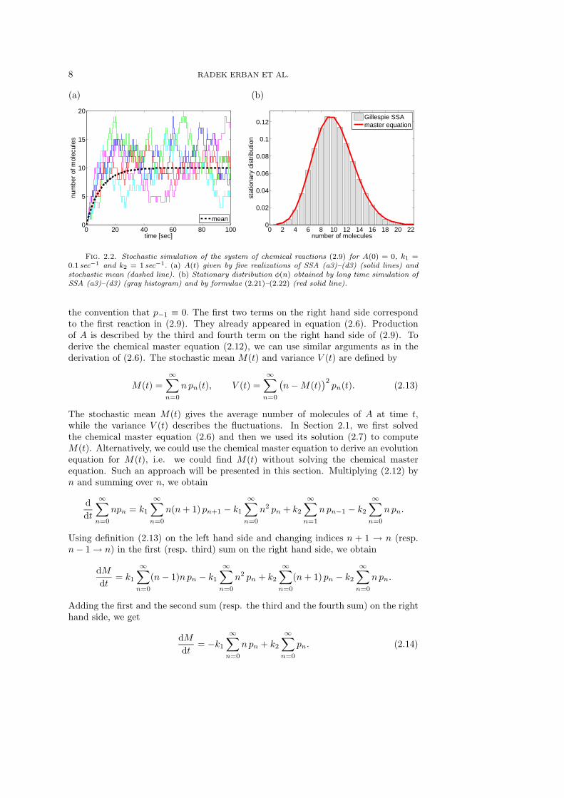
Five realizations of SSA (a3)–(d3) are presented in Figure 2.2(a) as solid lines. Weplot the number of molecules of A as a function of time for A(0) = 0, k1 = 0.1 sec−1
and k2 = 1 sec−1. We see that, after an initial transient, the number of molecules A(t)fluctuates around its mean value. To compute the stochastic mean and quantify thestochastic fluctuations, we use the chemical master equation which can be written forthe chemical system (2.9) in the following form
dpn
dt= k1(n + 1) pn+1 − k1n pn + k2 pn−1 − k2 pn (2.12)
where pn(t) denotes the probability that A(t) = n for n = 0, 1, 2, 3, . . . . Let us notethat the third term on the right hand side is missing in (2.12) for n = 0; i.e. we use
8 RADEK ERBAN ET AL.
(a)
0 20 40 60 80 1000
5
10
15
20
time [sec]
num
ber
of m
olec
ules
mean
(b)
0 2 4 6 8 10 12 14 16 18 20 220
0.02
0.04
0.06
0.08
0.1
0.12
number of molecules
stat
iona
ry d
istr
ibut
ion
Gillespie SSAmaster equation
Fig. 2.2. Stochastic simulation of the system of chemical reactions (2.9) for A(0) = 0, k1 =0.1 sec−1 and k2 = 1 sec−1. (a) A(t) given by five realizations of SSA (a3)–(d3) (solid lines) andstochastic mean (dashed line). (b) Stationary distribution φ(n) obtained by long time simulation ofSSA (a3)–(d3) (gray histogram) and by formulae (2.21)–(2.22) (red solid line).
the convention that p−1 ≡ 0. The first two terms on the right hand side correspondto the first reaction in (2.9). They already appeared in equation (2.6). Productionof A is described by the third and fourth term on the right hand side of (2.9). Toderive the chemical master equation (2.12), we can use similar arguments as in thederivation of (2.6). The stochastic mean M(t) and variance V (t) are defined by
M(t) =∞∑
n=0
n pn(t), V (t) =∞∑
n=0
(
n − M(t))2
pn(t). (2.13)
The stochastic mean M(t) gives the average number of molecules of A at time t,while the variance V (t) describes the fluctuations. In Section 2.1, we first solvedthe chemical master equation (2.6) and then we used its solution (2.7) to computeM(t). Alternatively, we could use the chemical master equation to derive an evolutionequation for M(t), i.e. we could find M(t) without solving the chemical masterequation. Such an approach will be presented in this section. Multiplying (2.12) byn and summing over n, we obtain
d
dt
∞∑
n=0
npn = k1
∞∑
n=0
n(n + 1) pn+1 − k1
∞∑
n=0
n2 pn + k2
∞∑
n=1
n pn−1 − k2
∞∑
n=0
n pn.
Using definition (2.13) on the left hand side and changing indices n + 1 → n (resp.n − 1 → n) in the first (resp. third) sum on the right hand side, we obtain
dM
dt= k1
∞∑
n=0
(n − 1)n pn − k1
∞∑
n=0
n2 pn + k2
∞∑
n=0
(n + 1) pn − k2
∞∑
n=0
n pn.
Adding the first and the second sum (resp. the third and the fourth sum) on the righthand side, we get
dM
dt= −k1
∞∑
n=0
n pn + k2
∞∑
n=0
pn. (2.14)

STOCHASTIC REACTION-DIFFUSION PROCESSES 9
Since pn(t) is the probability that A(t) = n and A(t) is equal to a nonnegative integerwith probability 1, we have
∞∑
n=0
pn(t) = 1. (2.15)
Using this fact together with the definition of M(t), equation (2.14) implies the evo-lution equation for M(t) in the form
dM
dt= −k1M + k2. (2.16)
The solution of (2.16) with initial condition M(0) = 0 is plotted as a dashed linein Figure 2.2(a). To derive the evolution equation for the variance V (t), let us firstobserve that definition (2.13) implies
∞∑
n=0
n2 pn(t) = V (t) + M(t)2. (2.17)
Multiplying (2.12) by n2 and summing over n, we obtain
d
dt
∞∑
n=0
n2pn = k1
∞∑
n=0
n2(n + 1) pn+1 − k1
∞∑
n=0
n3 pn + k2
∞∑
n=1
n2 pn−1 − k2
∞∑
n=0
n2 pn.
Changing indices n + 1 → n (resp. n − 1 → n) in the first (resp. third) sum on theright hand side and adding the first and the second sum (resp. the third and thefourth sum) on the right hand side, we get
d
dt
∞∑
n=0
n2pn = k1
∞∑
n=0
(−2n2 + n) pn + k2
∞∑
n=0
(2n + 1) pn.
Using (2.17), (2.15) and (2.13), we obtain
dV
dt+ 2M
dM
dt= −2k1
[
V + M2]
+ k1M + 2k2M + k2.
Substituting (2.16) for dM/dt, we derive the evolution equation for the variance V (t)in the following form
dV
dt= −2k1V + k1M + k2. (2.18)
The time evolution of M(t) and V (t) is described by (2.16) and (2.18). Let us definethe stationary values of M(t) and V (t) by
Ms = limt→∞
M(t), Vs = limt→∞
V (t). (2.19)
The values of Ms and Vs can be computed using the steady state equations corre-sponding to (2.16) and (2.18), namely by solving
0 = −k1Ms + k2, and 0 = −2k1Vs + k1Ms + k2.

10 RADEK ERBAN ET AL.
Consequently,
Ms = Vs =k2
k1.
For our parameter values k1 = 0.1 sec−1 and k2 = 1 sec−1, we obtain Ms = Vs = 10.We see in Figure 2.2(a) that A(t) fluctuates after a sufficiently long time around themean value Ms = 10. To quantify the fluctuations, one often uses the square root ofVs, the so-called mean standard deviation which is equal to
√10.
More detailed information about the fluctuations is given by the so-called sta-
tionary distribution φ(n), n = 0, 1, 2, 3, . . . , which is defined as
φ(n) = limt→∞
pn(t). (2.20)
This means that φ(n) is the probability that A(t) = n after an (infinitely) longtime. One way to compute φ(n) is to run SSA (a3)–(d3) for a long time and createa histogram of values of A(t) at given time intervals. Using k1 = 0.1 sec−1 andk2 = 1 sec−1, the results of such a long time computation are presented in Figure2.2(b) as a gray histogram. To compute it, we ran SSA (a3)–(d3) for 105 seconds,recording the value of A(t) every second and then dividing the whole histogram bythe number of recordings, i.e. by 105. An alternative way to compute φ(n) is to usethe steady state version of the chemical master equation (2.12), namely
0 = k1 φ(1) − k2 φ(0)
0 = k1(n + 1)φ(n + 1) − k1nφ(n) + k2 φ(n − 1) − k2 φ(n), for n ≥ 1,
which implies
φ(1) =k2
k1φ(0), (2.21)
φ(n + 1) =1
k1(n + 1)
[
k1nφ(n) + k2 φ(n) − k2 φ(n − 1)]
, for n ≥ 1. (2.22)
Consequently, we can express φ(n) for any n ≥ 1 in terms of φ(0). The formulae(2.21)–(2.22) yield an alternative way to compute φ(n). We put φ(0) = 1 and wecompute φ(n), for sufficiently many n, by (2.21)–(2.22). Then we divide φ(n), n ≥ 0,by
∑
φ(n). The results obtained by (2.21)–(2.22) are plotted in Figure 2.2(b) as a(red) solid line. As expected, the results compare well with the results obtained bythe long time stochastic simulation.
We can also find the formula for φ(n) directly. We let a reader to verify that thesolution of the recurrence formula (2.21)–(2.22) can be written as
φ(n) =C
n!
(
k2
k1
)n
(2.23)
where C is a real constant. Using (2.15) and (2.20), we have
∞∑
n=0
φ(n) = 1. (2.24)
Substituting (2.23) into the normalization condition (2.24), we get
1 =
∞∑
n=0
C
n!
(
k2
k1
)n
= C
∞∑
n=0
1
n!
(
k2
k1
)n
= C exp
[
k2
k1
]

STOCHASTIC REACTION-DIFFUSION PROCESSES 11
where we used the Taylor series for the exponential function to get the last equal-ity. Consequently, C = exp[−k2/k1] which, together with (2.23), implies that thestationary distribution φ(n) is the Poisson distribution
φ(n) =1
n!
(
k2
k1
)n
exp
[
−k2
k1
]
. (2.25)
Thus the red solid line in Figure 2.2(b) which was obtained numerically by the re-currence formula (2.21)–(2.22) can be also viewed as the stationary distribution φ(n)given by the explicit exact formula (2.25).
2.3. Gillespie algorithm. SSAs (a2)–(c2) and (a3)–(d3) were special forms ofthe so-called Gillespie SSA. In this section, we present this algorithm for a more com-plicated illustrative example which will also involve second-order chemical reactions.Such chemical reactions are of the following form
A + Ak1−→ C, A + B
k2−→ D. (2.26)
In the first equation, two molecules of A react with rate constant k1 to produceC. The probability that the reaction takes place in the time interval [t, t + dt) isequal to A(t)(A(t)− 1)k1dt. We define the propensity function of the first reaction asα1(t) = A(t)(A(t) − 1)k1. Then the probability that the first reaction occurs in thetime interval [t, t+dt) is equal to α1(t) dt. The propensity function which correspondsto the second equation in (2.26) is defined as α2(t) = A(t)B(t)k1 and the probabilitythat the second reaction occurs in the time interval [t, t + dt) is equal to α2(t) dt. Insuch a case, one molecule of A and one molecule of B react to form a molecule ofD. In general, the propensity function can be defined for any chemical reaction sothat its product with dt gives the probability that the given reaction occurs in theinfinitesimally small time interval [t, t + dt).
We consider that A and B can react according to (2.26). Moreover, we assumethat they are also produced with constant rates, that is, we consider a system of fourchemical equations:
A + Ak1−→ ∅ A + B
k2−→ ∅ (2.27)
∅ k3−→ A ∅ k4−→ B. (2.28)
Let us note that we are not interested in chemical species C and D. Hence, wereplaced them by ∅, consistent with our previous notation of unimportant chemicalspecies. To simulate the system of chemical reactions (2.27)–(2.28), we perform thefollowing four steps at time t (starting with A(0) = n0, B(0) = m0 at time t = 0):
(a4) Generate two random numbers r1, r2 uniformly distributed in (0, 1).
(b4) Compute the propensity functions of each reaction by α1 = A(t)(A(t)−1)k1,α2 = A(t)B(t)k2, α3 = k3 and α4 = k4. Compute α0 = α1 + α2 + α3 + α4.
(c4) Compute the time when the next chemical reaction takes place as t+τ where
τ =1
α0ln
[
1
r1
]
. (2.29)

12 RADEK ERBAN ET AL.
(a)
0 20 40 60 80 1000
5
10
15
20
25
time [sec]
num
ber
of A
mol
ecul
es
solution of ODEs
(b)
0 20 40 60 80 1000
5
10
15
20
25
time [sec]
num
ber
of B
mol
ecul
es
solution of ODEs
Fig. 2.3. Five realizations of SSA (a4)–(d4). Number of molecules of chemical species A(left panel) and B (right panel) are plotted as functions of time as solid lines. Different colourscorrespond to different realizations. The solution of (2.33)–(2.34) is given by the dashed line. Weuse A(0) = 0, B(0) = 0, k1 = 10−3 sec−1, k2 = 10−2 sec−1, k3 = 1.2 sec−1 and k4 = 1 sec−1.
(d4) Compute the number of molecules at time t + τ by
A(t + τ) =
A(t) − 2 if 0 ≤ r2 < α1/α0;A(t) − 1 if α1/α0 ≤ r2 < (α1 + α2)/α0;A(t) + 1 if (α1 + α2)/α0 ≤ r2 < (α1 + α2 + α3)/α0;
A(t) if (α1 + α2 + α3)/α0 ≤ r2 < 1;
(2.30)
B(t + τ) =
B(t) if 0 ≤ r2 < α1/α0;B(t) − 1 if α1/α0 ≤ r2 < (α1 + α2)/α0;
B(t) if (α1 + α2)/α0 ≤ r2 < (α1 + α2 + α3)/α0;B(t) + 1 if (α1 + α2 + α3)/α0 ≤ r2 < 1;
(2.31)
Then continue with step (a4) for time t + τ.
SSA (a4)–(d4) is a direct generalisation of SSA (a3)–(d3). At each time step, wefirst ask the question when will the next reaction occur? The answer is given byformula (2.29) which can be justified using the same arguments as formulae (2.5) or(2.10). Then we ask the question which reaction takes place. The probability thatthe i-th chemical reaction occurs is given by αi/α0. The decision which reaction takesplace is given in step (d4) with the help of the second uniformly distributed randomnumber r2. Knowing that the i-th reaction took place, we update the number ofreactants and products accordingly. Results of five realizations of SSA (a4)–(d4) areplotted in Figure 2.3 as solid lines. We use A(0) = 0, B(0) = 0, k1 = 10−3 sec−1,k2 = 10−2 sec−1, k3 = 1.2 sec−1 and k4 = 1 sec−1. We plot the number of moleculesof chemical species A and B as functions of time. We see that, after initial transients,A(t) and B(t) fluctuate around their average values. They can be estimated fromlong time stochastic simulations as 9.6 for A and 12.2 for B.
Let pn,m(t) be the probability that A(t) = n and B(t) = m. The chemical master

STOCHASTIC REACTION-DIFFUSION PROCESSES 13
equation can be written in the following form
dpn,m
dt= k1(n + 2)(n + 1) pn+2,m − k1n(n − 1) pn,m
+ k2(n + 1)(m + 1) pn+1,m+1 − k2nmpn,m
+ k3 pn−1,m − k3 pn,m + k4 pn,m−1 − k4 pn,m (2.32)
for n, m ≥ 0, with the convention that pn,m ≡ 0 if n < 0 or m < 0. The firstdifference between (2.32) and the chemical master equations from the previous sectionsis that equation (2.32) is parametrised by two indices n and m. The second importantdifference is that (2.32) cannot be solved analytically as we did with (2.6). Moreover,it does not lead to closed evolution equations for stochastic means and variances; i.e.we cannot follow the same technique as in the case of equation (2.12). The approachfrom the previous section does not work. Let us note that the probability pn,m(t) issometimes denoted by p(n,m, t); such a notational convention is often used when weconsider systems of many chemical species. We will use it in the following sections toavoid long subscripts.
The classical deterministic description of the chemical system (2.27)–(2.28) isgiven by the system of ODEs
da
dt= −2k1a
2 − k2 ab + k3, (2.33)
db
dt= −k2 ab + k4. (2.34)
The solution of (2.33)–(2.34) with initial conditions a(0) = 0 and b(0) = 0 is plottedas a dashed line in Figure 2.3. Let us note that the equations (2.33)–(2.34) do notdescribe the stochastic means of A(t) and B(t). For example, the steady state valuesof (2.33)–(2.34) are (for the parameter values of Figure 2.3) equal to as = bs = 10. Onthe other hand, the average values estimated from long time stochastic simulations are9.6 for A and 12.2 for B. We will see later in Section 5.1 that the difference betweenthe results of stochastic simulations and the corresponding ODEs can be even moresignificant.
The stationary distribution is defined by
φ(n,m) = limt→∞
pn,m(t).
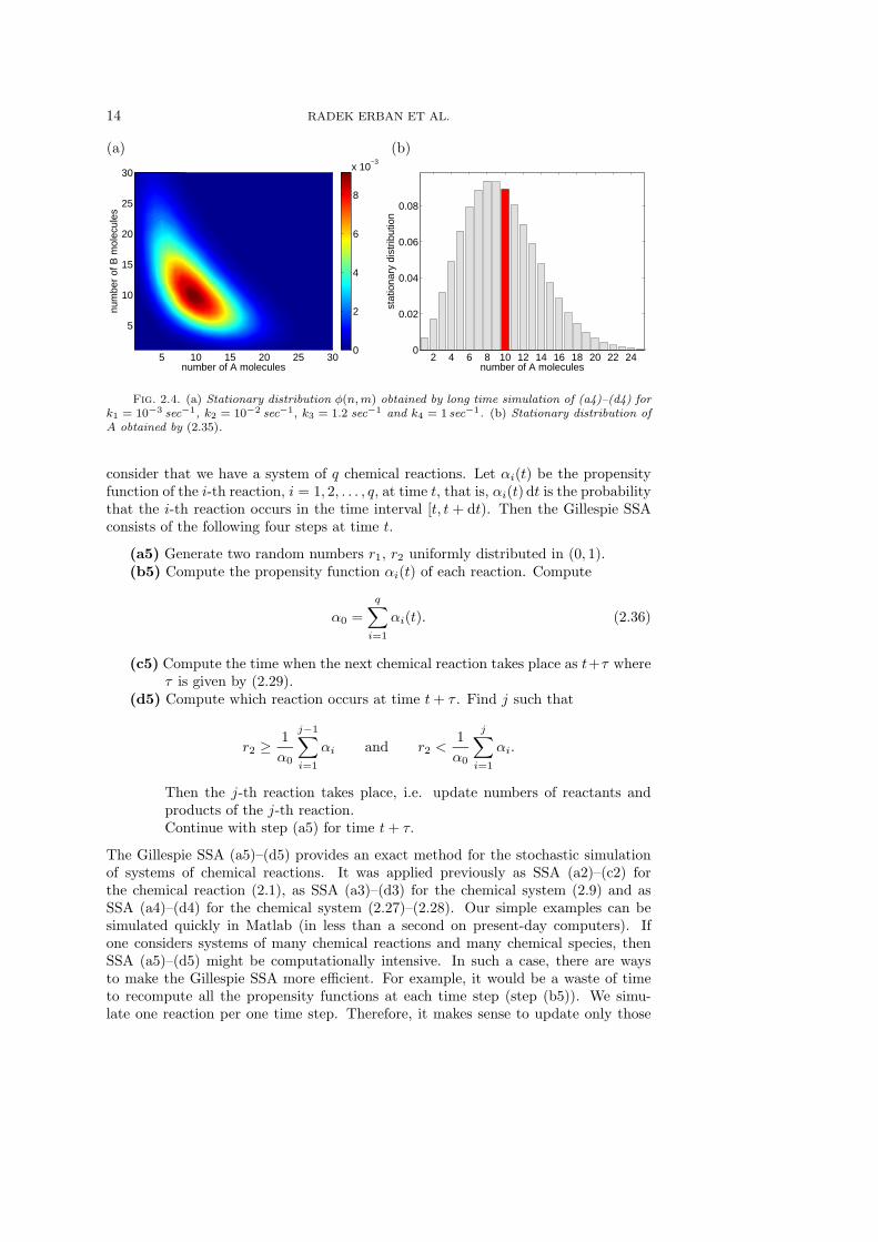
This can be computed by long time simulations of SSA (a4)–(d4) and is plotted inFigure 2.4(a). We see that there is a correlation between the values of A and B. Thiscan also be observed in Figure 2.3. Looking at the blue realizations, we see that thevalues of A(t) are below the average and the values of B(t) are above the average,similarly for other realizations. One can also define the stationary distribution of Aonly by
φ(n) =
∞∑
m=0
φ(n,m). (2.35)
Summing the results of Figure 2.4(a) over m, we obtain φ(n) which is plotted in Figure2.4(b) as a gray histogram. The red bar highlights the steady state value as = 10 ofsystem (2.33)–(2.34).
SSAs (a3)–(d3) and (a4)–(d4) were special forms of the so-called Gillespie SSA.To conclude this section, we formulate the Gillespie SSA in its full generality. Let us
14 RADEK ERBAN ET AL.
(a)
number of A molecules
num
ber
of B
mol
ecul
es
5 10 15 20 25 30
5
10
15
20
25
30
0
2
4
6
8
x 10−3
(b)
2 4 6 8 10 12 14 16 18 20 22 240
0.02
0.04
0.06
0.08
number of A molecules
stat
iona
ry d
istr
ibut
ion
Fig. 2.4. (a) Stationary distribution φ(n, m) obtained by long time simulation of (a4)–(d4) fork1 = 10−3 sec−1, k2 = 10−2 sec−1, k3 = 1.2 sec−1 and k4 = 1 sec−1. (b) Stationary distribution ofA obtained by (2.35).
consider that we have a system of q chemical reactions. Let αi(t) be the propensityfunction of the i-th reaction, i = 1, 2, . . . , q, at time t, that is, αi(t) dt is the probabilitythat the i-th reaction occurs in the time interval [t, t + dt). Then the Gillespie SSAconsists of the following four steps at time t.
(a5) Generate two random numbers r1, r2 uniformly distributed in (0, 1).(b5) Compute the propensity function αi(t) of each reaction. Compute
α0 =
q∑
i=1
αi(t). (2.36)
(c5) Compute the time when the next chemical reaction takes place as t+τ whereτ is given by (2.29).
(d5) Compute which reaction occurs at time t + τ . Find j such that
r2 ≥ 1
α0
j−1∑
i=1
αi and r2 <1
α0
j∑
i=1
αi.
Then the j-th reaction takes place, i.e. update numbers of reactants andproducts of the j-th reaction.Continue with step (a5) for time t + τ.
The Gillespie SSA (a5)–(d5) provides an exact method for the stochastic simulationof systems of chemical reactions. It was applied previously as SSA (a2)–(c2) forthe chemical reaction (2.1), as SSA (a3)–(d3) for the chemical system (2.9) and asSSA (a4)–(d4) for the chemical system (2.27)–(2.28). Our simple examples can besimulated quickly in Matlab (in less than a second on present-day computers). Ifone considers systems of many chemical reactions and many chemical species, thenSSA (a5)–(d5) might be computationally intensive. In such a case, there are waysto make the Gillespie SSA more efficient. For example, it would be a waste of timeto recompute all the propensity functions at each time step (step (b5)). We simu-late one reaction per one time step. Therefore, it makes sense to update only those

STOCHASTIC REACTION-DIFFUSION PROCESSES 15
(a)
−0.6 −0.4 −0.2 0 0.2 0.4 0.6
−0.6
−0.4
−0.2
0
0.2
0.4
0.6
x [mm]
y [m
m]
(b)
x [mm]
y [m
m]
−0.6 −0.4 −0.2 0 0.2 0.4 0.6
−0.6
−0.4
−0.2
0
0.2
0.4
0.6
0.2
0.4
0.6
0.8
1
1.2
Fig. 3.1. (a) Six trajectories obtained by SSA (a6)–(b6) for D = 10−4 mm2 sec−1 and∆t = 0.1 sec. Trajectories were started at the origin and followed for 10 minutes. (b) Probabilitydistribution function ψ(x, y, t) given by (3.5) at time t = 10 min.
propensity functions which are changed by the chemical reaction which was selected instep (d5) of SSA (a5)–(d5). A more detailed discussion about the efficient computerimplementation of the Gillespie SSA can be found e.g. in [16].
3. Diffusion. Diffusion is the random migration of molecules (or small particles)arising from motion due to thermal energy [3]. As shown by Einstein, the kinetic en-ergy of a molecule (e.g. protein) is proportional to the absolute temperature. Inparticular, the protein molecule has a non-zero instantaneous speed at, for exam-ple, room temperature or at the temperature of the human body. A typical proteinmolecule is immersed in the aqueous medium of a living cell. Consequently, it can-not travel too far before it bumps into other molecules (e.g. water molecules) in thesolution. As a result, the trajectory of the molecule is not straight but it executesa random walk as shown in Figure 3.1(a). We plot six possible trajectories of theprotein molecule with six different colours. All trajectories start at the origin and arefollowed for 10 minutes. We will provide more details about this figure together withthe methods for simulating molecular diffusion in the rest of this section. Stochasticmodels of diffusion which are based on the Smoluchowski equation are introduced inSection 3.1. In Section 3.2, we introduce a model which is suitable for coupling withthe Gillespie SSA. Both modelling approaches will be used later in Section 4 for thestochastic modelling of reaction-diffusion processes. Let us note that there exist othermodels of molecular diffusion – they will be discussed in Section 6.
3.1. Smoluchowski equation and diffusion. Let [X(t), Y (t), Z(t)] ∈ R3 be
the position of a diffusing molecule at time t. Starting with [X(0), Y (0), Z(0)] =[x0, y0, z0], we want to compute the time evolution of [X(t), Y (t), Z(t)]. To do that, wemake use of a generator of random numbers which are normally distributed with zeromean and unit variance. Such a generator is part of many modern computer languages(e.g. function randn in Matlab). Diffusive spreading of molecules is characterised bya single diffusion constant D which depends on the size of the molecule, absolutetemperature and viscosity of the solution [3]. Choosing time step ∆t, we computethe time evolution of the position of the diffusing molecule by performing two stepsat time t:

16 RADEK ERBAN ET AL.
(a6) Generate three normally distributed (with zero mean and unit variance)random numbers ξx, ξy and ξz.
(b6) Compute the position of the molecule at time t + ∆t by
X(t + ∆t) = X(t) +√
2D ∆t ξx, (3.1)
Y (t + ∆t) = Y (t) +√
2D ∆t ξy, (3.2)
Z(t + ∆t) = Z(t) +√
2D ∆t ξz, (3.3)
Then continue with step (a6) for time t + ∆t.
Choosing D = 10−4 mm2 sec−1 (diffusion constant of a typical protein molecule),[X(0), Y (0), Z(0)] = [0, 0, 0] and ∆t = 0.1 sec, we plot six realizations of SSA (a6)–(b6) in Figure 3.1(a). We plot only the x and y coordinates. We follow the diffusingmolecule for 10 minutes. The position of the molecule at time t = 10 min is denotedas a black circle for each trajectory.
Equations (3.1)–(3.3) are discretized versions of stochastic differential equations(SDEs) which are sometimes called Smoluchowski equations. Some basic facts aboutSDEs can be found e.g. in [2, 14]. A more accessible introduction to SDEs can befound in [23] which has a similar philosophy as our paper. Reference [23] is a nicealgorithmic introduction to SDEs for students who do not have a prior knowledgeof advanced probability theory or stochastic analysis. We will not go into details ofSDEs in this paper, but only highlight some interesting facts which will be usefullater.
First, equations (3.1)–(3.3) are not coupled. To compute the time evolution ofX(t), we do not need to know the time evolution of Y (t) or Z(t). We will later focusonly on the time evolution of the x-th coordinate, effectively studying one-dimensionalproblems. Two-dimensional or three-dimensional problems can be treated similarly.Second, we see that different realizations of SSA (a6)–(b6) give different results. To getmore reproducible quantities, we will shortly study the behaviour of several molecules.However, even in the case of a single diffusing molecule, there are still quantitieswhose evolution is deterministic. Let ϕ(x, y, t) dxdydz be the probability that X(t) ∈[x, x + dx), Y (t) ∈ [y, y + dy) and Z(t) ∈ [z, z + dz) at time t. It can be shown thatϕ evolves according to the partial differential equation
∂ϕ
∂t= D
(
∂2ϕ
∂x2+
∂2ϕ
∂y2+
∂2ϕ
∂z2
)
, (3.4)
which is a special form of the so-called Fokker-Planck equation. Since our random walkstarts at the origin, we can solve (3.4) with initial condition ϕ(x, y, z, 0) = δ(x, y, z)where δ is the Dirac distribution at the origin. We obtain
ϕ(x, y, z, t) =1
(4Dπt)3/2exp
[
−x2 + y2 + z2
4Dt
]
.
In order to visualise this probability distribution function, we integrate it over z toget probability distribution function
ψ(x, y, t) =
∫
R
ϕ(x, y, z, t)dz =1
4Dπtexp
[
−x2 + y2
4Dt
]
. (3.5)
This means that ψ(x, y, t) dxdy is the probability that X(t) ∈ [x, x + dx) and Y (t) ∈[y, y + dy) at time t. The function ψ(x, y, t) at time t = 10 min is plotted in Figure

STOCHASTIC REACTION-DIFFUSION PROCESSES 17
(a)
0 0.2 0.4 0.6 0.8 10
2
4
6
8
10
12
14
x [mm]
time
[min
]
(b)
0 0.2 0.4 0.6 0.8 10
10
20
30
40
50
60time=4 min
x [mm]
num
ber
of m
olec
ules
in c
ompa
rtm
ent
mean
0
0.5
1
1.5
2
conc
entr
atio
n in
[mol
ecul
es/µ
m]
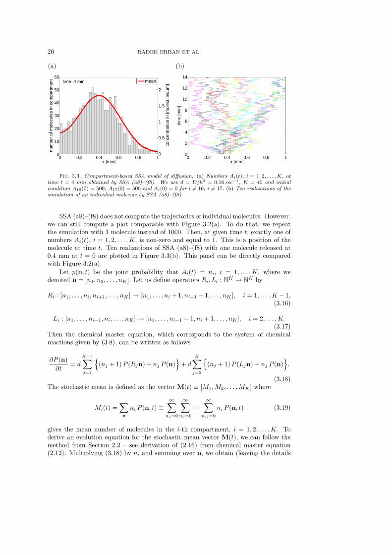
Fig. 3.2. (a) Ten trajectories computed by SSA (a7)–(c7) for D = 10−4 mm2 sec−1, L = 1mm, X(0) = 0.4 mm and ∆t = 0.1 sec. (b) Numbers of molecules in bins of length h = 25 µm attime t = 4 min.
3.1(b). It can be obtained also by computing many realizations of SSA (a6)–(b6) andplotting the histogram of positions of a molecule at time 10 min; such positions weredenoted as black circles for the six illustrative trajectories in Figure 3.1(a).
One important issue which was not addressed previously is that molecules diffusein bounded volumes, i.e. the domain of interest has boundaries and suitable bound-ary conditions must be implemented. In the rest of this paper, we focus on one-dimensional problems to avoid technicalities. Hence, we effectively study diffusion ofmolecules in the one-dimensional interval [0, L]. Then the SSA can be formulated asfollows:
(a7) Generate a normally distributed (with zero mean and unit variance) randomnumber ξ.
(b7) Compute the position of the molecule at time t + ∆t by
X(t + ∆t) = X(t) +√
2D ∆t ξ. (3.6)
(c7) If X(t + ∆t) computed by (3.6) is less than 0, thenX(t + ∆t) = −X(t) −
√2D ∆t ξ.
If X(t + ∆t) computed by (3.6) is greater than L, thenX(t + ∆t) = 2L − X(t) −
√2D ∆t ξ.
Then continue with step (a7) for time t + ∆t.
The boundary condition implemented in step (c7) is the so-called reflective boundary
condition or zero flux boundary condition. It can be used when there is no chem-ical interaction between the boundary and diffusing molecules. More complicatedboundary conditions are discussed in [7, 8].
Choosing D = 10−4 mm2 sec−1, L = 1 mm, X(0) = 0.4 mm and ∆t = 0.1 sec, weplot ten realizations of SSA (a7)–(c7) in Figure 3.2(a). Let us assume that we havea system of 1000 molecules which are released at position x = 0.4 mm at time t = 0.Then Figure 3.2(a) can be viewed as a plot of the trajectories of ten representativemolecules. Considering 1000 molecules, the trajectories of individual molecules areof no special interest. We are rather interested in spatial histograms (density ofmolecules). An example of such a plot is given in Figure 3.2(b). We simulate 1000

18 RADEK ERBAN ET AL.
molecules, each following SSA (a7)–(c7). At time t = 4 min, we divided the domainof interest [0, L] into 40 bins of length h = L/40 = 25 µm. We calculated the numberof molecules in each bin [(i − 1)h, ih), i = 1, 2, . . . , 40, at time t = 4 min and plottedthem as a histogram.
Let us note that the deterministic counterpart to the stochastic simulation is asolution of the corresponding Fokker-Planck equation (diffusion equation in our case)which, in one dimension with zero flux boundary conditions, reads as follows
∂ϕ
∂t= D
∂2ϕ
∂x2where
∂ϕ
∂x(0) =
∂ϕ
∂x(L) = 0. (3.7)
The solution of (3.7) with the Dirac-like initial condition at x = 0.4 mm is plotted asa red solid line in Figure 3.2(b) for comparison.
3.2. Compartment-based approach to diffusion. In Section 3.1, we sim-ulated the behaviour of 1000 molecules by computing the individual trajectories ofevery molecule (using SSA (a7)–(c7)). At the end of the simulation, we divided thecomputational domain [0, L] into K = 40 compartments and we plotted numbers ofmolecules in each compartment in Figure 3.2(b). In particular, most of the com-puted information (1000 trajectories) was not used for the final result – the spatialhistogram. We visualised only 40 numbers (numbers of molecules in compartments)instead of 1000 computed positions of molecules. In this section, we present a differentSSA for the simulation of molecular diffusion. We redo the example from Section 3.1but instead of simulating 1000 positions of the individual molecules, we are going tosimulate directly the time evolution of 40 compartments.
To do that, we divide the computational domain [0, L] into K = 40 compartmentsof length h = L/K = 25µm. We denote the number of molecules of chemical speciesA in the i-th compartment [(i − 1)h, ih) by Ai, i = 1, . . . ,K. We apply the GillespieSSA to the following chain of “chemical reactions”:
A1
d−→←−d
A2
d−→←−d
A3
d−→←−d
. . .d−→←−d
AK (3.8)
where
Ai
d−→←−d
Ai+1 means that Aid−→ Ai+1 and Ai+1
d−→ Ai.
We will shortly show that the Gillespie SSA of (3.8) provides a correct model ofdiffusion provided that the rate constant d in (3.8) is chosen as d = D/h2 whereD is the diffusion constant and h is the compartment length. The compartment-based SSA can be described as follows. Starting with initial condition Ai(t) = a0,i,i = 1, 2, . . . ,K, we perform six steps at time t:
(a8) Generate two random numbers r1, r2 uniformly distributed in (0, 1).(b8) Compute propensity functions of reactions by αi = Ai(t)d for i = 1, 2, . . . ,K.
Compute
α0 =
K−1∑
i=1
αi +
K∑
i=2
αi. (3.9)
(c8) Compute the time at which the next chemical reaction takes place as t + τwhere τ is given by (2.29).

STOCHASTIC REACTION-DIFFUSION PROCESSES 19
(d8) If r2 <∑K−1
i=1 αi/α0, then find j ∈ {1, 2, . . . ,K − 1} such that
r2 ≥ 1
α0
j−1∑
i=1
αi and r2 <1
α0
j∑
i=1
αi.
Then compute the number of molecules at time t + τ by
Aj(t + τ) = Aj(t) − 1, (3.10)
Aj+1(t + τ) = Aj+1(t) + 1, (3.11)
Ai(t + τ) = Ai(t), for i 6= j, i 6= j + 1. (3.12)
(e8) If r2 ≥ ∑K−1i=1 αi/α0, then find j ∈ {2, 3, . . . ,K} such that
r2 ≥ 1
α0
(
K−1∑
i=1
αi +
j−1∑
i=2
αi
)
and r2 <1
α0
(
K−1∑
i=1
αi +
j∑
i=2
αi
)
.
Then compute the number of molecules at time t + τ by
Aj(t + τ) = Aj(t) − 1, (3.13)
Aj−1(t + τ) = Aj−1(t) + 1, (3.14)
Ai(t + τ) = Ai(t), for i 6= j, i 6= j − 1. (3.15)
(f8) Continue with step (a8) for time t + τ.
The first term on the right hand side of (3.9) corresponds to reactions Ai → Ai+1
(jumps to the right) and the second term corresponds to reactions Ai → Ai−1 (jumpsto the left). The time of the next chemical reaction is computed in the step (c8) usingformula (2.29) derived previously. The decision about which reaction takes place isdone in steps (d8)–(e8) with the help of random number r2. Jumps to the right areimplemented in step (d8) and jumps to the left in step (e8).
We want to redo the example from Section 3.1, i.e. simulate 1000 moleculesstarting from position 0.4 mm in the interval [0, L] for L = 1 mm. We use K = 40.Since 0.4 mm is exactly a boundary between the 16th and 17th compartment, theinitial condition is given by A16(0) = 500, A17(0) = 500 and Ai(0) = 0 for i 6= 16,i 6= 17. As D = 10−4 mm2 sec−1, we have d = D/h2 = 0.16 sec−1. The numbers Ai(t),i = 1, . . . ,K, at time t = 4 min, are plotted in Figure 3.3(a) as a histogram. This panelcan be directly compared with Figure 3.2(b). The computational intensity of SSA(a8)–(f8) can be decreased using the appropriate way to implement it in the computer.For example, only one chemical reaction occurs per time step. Consequently, onlytwo propensity functions change and need to be updated in step (b8). Moreover, theformula (3.9) can be simplifed as follows
α0 =
K−1∑
i=1
αi +
K∑
i=2
αi = 2
K∑
i=1
αi−α1−αK = 2d
K∑
i=1
Ai(t)−α1−αK = 2dN −α1−αK ,
where N = 1000 is the total number of molecules in the simulation (this number isconserved because there is no creation or degradation of the molecules in the system).Hence, we need to recompute α0 only when there is a change in α1 or αK , i.e. wheneverthe boundary compartments were involved in the previous reaction.
20 RADEK ERBAN ET AL.
(a)
0 0.2 0.4 0.6 0.8 10
10
20
30
40
50
60time=4 min
x [mm]
num
ber
of m
olec
ules
in c
ompa
rtm
ent
mean
0
0.5
1
1.5
2
conc
entr
atio
n in
[mol
ecul
es/µ
m]
(b)
0 0.2 0.4 0.6 0.8 10
2
4
6
8
10
12
14
x [mm]
time
[min
]Fig. 3.3. Compartment-based SSA model of diffusion. (a) Numbers Ai(t), i = 1, 2, . . . , K, at
time t = 4 min obtained by SSA (a8)–(f8). We use d = D/h2 = 0.16 sec−1, K = 40 and initialcondition A16(0) = 500, A17(0) = 500 and Ai(0) = 0 for i 6= 16, i 6= 17. (b) Ten realizations of thesimulation of an individual molecule by SSA (a8)–(f8).
SSA (a8)–(f8) does not compute the trajectories of individual molecules. However,we can still compute a plot comparable with Figure 3.2(a). To do that, we repeatthe simulation with 1 molecule instead of 1000. Then, at given time t, exactly one ofnumbers Ai(t), i = 1, 2, . . . ,K, is non-zero and equal to 1. This is a position of themolecule at time t. Ten realizations of SSA (a8)–(f8) with one molecule released at0.4 mm at t = 0 are plotted in Figure 3.3(b). This panel can be directly comparedwith Figure 3.2(a).
Let p(n, t) be the joint probability that Ai(t) = ni, i = 1, . . . ,K, where wedenoted n = [n1, n2, . . . , nK ]. Let us define operators Ri, Li : N
K → NK by
Ri : [n1, . . . , ni, ni+1, . . . , nK ] → [n1, . . . , ni + 1, ni+1 − 1, . . . , nK ], i = 1, . . . ,K − 1,(3.16)
Li : [n1, . . . , ni−1, ni, . . . , nK ] → [n1, . . . , ni−1 − 1, ni + 1, . . . , nK ], i = 2, . . . ,K.(3.17)
Then the chemical master equation, which corresponds to the system of chemicalreactions given by (3.8), can be written as follows
∂P (n)
∂t= d
K−1∑
j=1
{
(nj + 1)P (Rjn) − nj P (n)}
+ d
K∑
j=2
{
(nj + 1)P (Ljn) − nj P (n)}
.
(3.18)The stochastic mean is defined as the vector M(t) ≡ [M1,M2, . . . ,MK ] where
Mi(t) =∑
n
ni P (n, t) ≡∞∑
n1=0
∞∑
n2=0
· · ·∞∑
nK=0
ni P (n, t) (3.19)
gives the mean number of molecules in the i-th compartment, i = 1, 2, . . . ,K. Toderive an evolution equation for the stochastic mean vector M(t), we can follow themethod from Section 2.2 – see derivation of (2.16) from chemical master equation(2.12). Multiplying (3.18) by ni and summing over n, we obtain (leaving the details

STOCHASTIC REACTION-DIFFUSION PROCESSES 21
to the student) a system of equations for Mi of the form
∂Mi
∂t= d(Mi+1 + Mi−1 − 2Mi), i = 2, . . . ,K − 1, (3.20)
∂M1
∂t= d(M2 − M1),
∂MK
∂t= d(MK−1 − MK). (3.21)
System (3.20)–(3.21) is equivalent to a discretization of (3.7) provided that d = D/h2.Hence, we have derived the relation between the rate constant d in (3.8), diffusionconstant D and compartment length h. The solution of (3.7) with the Dirac-likeinitial condition at x = 0.4 mm is plotted for comparison as a red solid line in Figure3.3(a).
The noise is described by the variance vector V(t) ≡ [V1, V2, . . . , VK ] where
Vi(t) =∑
n
(ni − Mi(t))2 P (n, t) ≡
∞∑
n1=0
∞∑
n2=0
· · ·∞∑
nK=0
(ni − Mi(t))2 P (n, t) (3.22)
gives the variance of number of molecules in the i-th compartment, i = 1, 2, . . . ,K.To derive the evolution equation for the vector V(t), we define the matrix {Vi,j} by
Vij =∑
n
ninj P (n, t) − MiMj , for i, j = 1, 2, . . . ,K.
Using (3.22), we obtain Vi = Vii for i = 1, 2, . . . ,K. Multiplying (3.18) by n2i and
summing over n, we obtain
∂
∂t
∑
n
n2i P (n) = d
K−1∑
j=1
{
∑
n
n2i (nj + 1)P (Rjn) −
∑
n
n2i nj P (n)
}
+ d
K∑
j=2
{
∑
n
n2i (nj + 1)P (Ljn) −
∑
n
n2i nj P (n)
}
. (3.23)
Let us assume that i = 2, . . . ,K − 1. Let us consider the term corresponding to j = iin the first sum on the right hand side. We get
∑
n
n2i (ni + 1)P (Rin) −
∑
n
n2i ni P (n) =
∑
n
(ni − 1)2ni P (n) −∑
n
n2i ni P (n)
=∑
n
(−2n2i + ni)P (n) = −2Vi − 2M2
i + Mi.
First, we changed indices in the first sum Rin → n and then we used definitions (3.19)and (3.22). Similarly, the term corresponding to j = i−1 in the first sum on the righthand side of (3.23) can be rewritten as
∑
n
n2i (ni−1 + 1)P (Ri−1n) −
∑
n
n2i ni−1 P (n) =
∑
n
(2nini−1 + ni−1)P (n)
= 2Vi,i−1 + 2MiMi−1 + Mi−1.
22 RADEK ERBAN ET AL.
Other terms (corresponding to j 6= i, i − 1) in the first sum on the right hand side of(3.23) are equal to zero. The second sum can be handled analogously. We obtain
∂
∂t
∑
n
n2i P (n) = d
{
2Vi,i−1 + 2MiMi−1 + Mi−1 − 2Vi − 2M2i + Mi
}
+ d{
2Vi,i+1 + 2MiMi+1 + Mi+1 − 2Vi − 2M2i + Mi
}
. (3.24)
Using (3.22) and (3.20) on the left hand side of (3.24), we obtain
∂
∂t
∑
n
n2i P (n) =
∂Vi
∂t+ 2Mi
∂Mi
∂t=
∂Vi
∂t+ d(2MiMi+1 + 2MiMi−1 − 4M2
i ).
Substituting this into (3.24), we get
∂Vi
∂t= 2d
{
Vi,i+1 + Vi,i−1 − 2Vi
}
+ d{
Mi+1 + Mi−1 + 2Mi
}
(3.25)
for i = 2, . . . ,K − 1. Similarly, we get
∂V1
∂t= 2d
{
V1,2 − V1
}
+ d{
M2 + M1
}
, (3.26)
∂VK
∂t= 2d
{
VK,K−1 − VK
}
+ d{
MK−1 + MK
}
. (3.27)
We see that the evolution equation for the variance vector V(t) depends on the meanM, variance V and on non-diagonal terms of the matrix Vi,j . To get a closed systemof equations, we have to derive evolution equations for Vi,j too. This can be doneby multiplying (3.18) by ninj , summing over n and following the same arguments asbefore. We conclude this section with some consequences of (3.20)–(3.21) and (3.25)–(3.27). Looking at the steady states of equations (3.20)–(3.21), we obtain Mi = N/K,i = 1, 2, . . . ,K, where N is the total number of diffusing molecules. Moreover, thevariance equations imply that Vi = N/K, i = 1, 2, . . . ,K, at the steady state.
4. Stochastic reaction-diffusion models. In this section, we add chemicalreactions to both models of molecular diffusion which were presented in Section 3.We introduce two methods for the stochastic modelling of reaction-diffusion processes.The first one is based on the diffusion model from Section 3.2, the second one on thediffusion model from Section 3.1. We explain both methods using the same example.Namely, we consider molecules (e.g. protein) which diffuse in the domain [0, L] withdiffusion constant D as we considered in Section 3. Moreover, we assume that proteinmolecules are degraded (in the whole domain) and produced in part of the domain,i.e. we consider the chemical reactions from Sections 2.1 and 2.2 in our illustrativereaction-diffusion model. The model has a realistic motivation which is discussed inmore detail later in Section 5.2. In Section 4.3, we present another illustrative exampleof a reaction-diffusion process incorporating the nonlinear model (2.27)–(2.28).
4.1. Compartment-based reaction-diffusion SSA. We consider moleculesof chemical species A which are diffusing in the domain [0, L], where L = 1 mm,with diffusion constant D = 10−4 mm2 sec−1. Initially, there are no molecules inthe system. Molecules are produced in the part of the domain [0, L/5] with rate

STOCHASTIC REACTION-DIFFUSION PROCESSES 23
(a)
0 0.2 0.4 0.6 0.8 10
20
40
60
80
100
x [mm]
num
ber
of m
olec
ules
time=10 min
mean
(b)
0 0.2 0.4 0.6 0.8 10
20
40
60
80
100
120
140
x [mm]
num
ber
of m
olec
ules
time=30 min
mean
Fig. 4.1. One realization of the Gillespie SSA (a5)–(d5) for the system of chemical reactions(4.1)–(4.3). Gray histograms show numbers of molecules in compartments at time: (a) t = 10 min;(b) t = 30 min. Solution of (4.9)–(4.10) is plotted as the red solid line.
kp = 0.012 µm−1 sec−1. This means that the probability that a molecule is createdin the subinterval of the length 1 µm is equal to kp dt. Consequently, the probabilitythat a molecule is created somewhere in the interval [0, L/5] is equal to kpL/5 dt.Molecules are degraded with rate k1 = 10−3 sec−1 according to the chemical reaction(2.1).
Following Section 3.2, we divide the computational domain [0, L] into K = 40compartments of length h = L/K = 25µm. We denote the number of molecules ofchemical species A in the i-th compartment [(i − 1)h, ih) by Ai, i = 1, . . . ,K. Thenour reaction-diffusion process is described by the system of chemical reactions
A1
d−→←−d
A2
d−→←−d
A3
d−→←−d
. . .d−→←−d
AK , (4.1)
Aik1−→ ∅, for i = 1, 2, . . . ,K, (4.2)
∅ k2−→ Ai, for i = 1, 2, . . . ,K/5. (4.3)
Equation (4.1) describes diffusion and is identical to (3.8). In particular, the rateconstant d is given by d = D/h2. Equation (4.2) describes the degradation of A andis, in fact, equation (2.1) applied to every compartment. Equation (4.3) describesthe production of A in the first K/5 compartments (e.g. in part [0, L/5] of thecomputational domain). The rate constant k2 describes the rate of production percompartment. Since each compartment has length h, we have k2 = kph.
The system of chemical reactions (4.1)–(4.3) is simulated using the Gillespie SSA(a5)–(d5). In our case, the propensity functions of reactions in (4.1) are given asAi(t)d, the propensity functions of reactions in (4.2) are given as Ai(t)k1 and propen-sity functions of reactions in (4.3) are equal to k2. Starting with no molecules of A inthe system, we compute one realization of SSA (a5)–(d5) for the system of reactions(4.1)–(4.3). We plot the numbers of molecules in compartments at two different timesin Figure 4.1.

24 RADEK ERBAN ET AL.
Let p(n, t) be the joint probability that Ai(t) = ni, i = 1, . . . ,K, where we usethe notation n = [n1, n2, . . . , nK ]. Let us define operators Ri, Li : N
K → NK by
(3.16)–(3.17). Then the chemical master equation, which corresponds to the systemof chemical reactions (4.1)–(4.3), can be written as follows
∂p(n)
∂t= d
K−1∑
i=1
{
(ni + 1) p(Rin) − ni p(n)}
+ d
K∑
i=2
{
(ni + 1) p(Lin) − ni p(n)}
+ k1
K∑
i=1
{
(ni + 1) p(n1, . . . , ni + 1, . . . , nK) − ni p(n)}
+ k2
K/5∑
i=1
{
p(n1, . . . , ni − 1, . . . , nK) − p(n)}
. (4.4)
The first two sums correspond to diffusion (4.1), the third sum to degradation (4.2)and the fourth sum to production (4.3). The stochastic mean is defined as the vectorM(t) ≡ [M1,M2, . . . ,MK ] where Mi is given by (3.19). This gives the mean numberof molecules in the i-th compartment, i = 1, 2, . . . ,K, at time t (averaged over manyrealizations of SSA (a5)–(d5)). To derive the evolution equation for the stochasticmean vector M(t), we can follow the method from Section 2.2 – see derivation of(2.16) from the chemical master equation (2.12). Multiplying (4.4) by ni and summingover all nj , j = 1, . . . ,K, we obtain (leaving the details to the student) a system ofequations for Mi in the form
∂M1
∂t= d(M2 − M1) + k2 − k1M1, (4.5)
∂Mi
∂t= d(Mi+1 + Mi−1 − 2Mi) + k2 − k1Mi, i = 2, . . . ,K/5, (4.6)
∂Mi
∂t= d(Mi+1 + Mi−1 − 2Mi) − k1Mi, i = K/5 + 1, . . . ,K − 1, (4.7)
∂MK
∂t= d(MK−1 − MK) − k1MK . (4.8)
System (4.5)–(4.8) is a discretized version of the reaction-diffusion equation
∂a
∂t= D
∂2a
∂x2+ k2χ[0,L/5] − k1a (4.9)
with zero-flux boundary conditions
∂a
∂x(0) =
∂a
∂x(L) = 0. (4.10)
Here, χ[0,L/5] is the characteristic function of the interval [0, L/5]. Using initial con-dition a(·, 0) ≡ 0, we computed the solution of (4.9)–(4.10) numerically. It is plottedas a red solid line in Figure 4.1 for comparison.
The concentration of molecules in the i-th compartment is defined as M i = Mi/h,i = 1, . . . ,K. Dividing (4.5)–(4.8) by h, we can write a system of ODEs for M i. It isa discretized version of the reaction-diffusion equation
∂a
∂t= D
∂2a
∂x2+ kpχ[0,L/5] − k1a (4.11)

STOCHASTIC REACTION-DIFFUSION PROCESSES 25
where a ≡ a(x, t) is the concentration of molecules of A at point x and time t. Theequation (4.11) provides a classical deterministic description of the reaction-diffusionprocess. Its parameters D, kp and k1 are independent of h. Solving (4.11) is equivalentto solving (4.9). Consequently, the red solid line in Figure 4.1 can be also viewed as aplot of ah where a is the solution of the classical deterministic model (4.11) with thezero-flux boundary conditions.
4.2. Reaction-diffusion SSA based on the Smoluchowski equation. Inthis section, we present a SSA which implements the Smoluchowski model of diffusionfrom Section 3.1, that is, we follow the trajectories of individual molecules. Diffusionof each molecule is modelled according to the model (a7)–(c7). We explain the SSAusing the reaction-diffusion example from Section 4.1. Choosing a small time step ∆t,we perform the following three steps at time t:
(a9) For each molecule, compute its position at time t + ∆t according to steps(a7)–(c7).
(b9) For each molecule, generate a random number r1 uniformly distributed inthe interval (0, 1). If r1 < k1 ∆t, then remove the molecule from the system.
(c9) Generate a random number r2 uniformly distributed in the interval (0, 1).If r2 < kpL/5∆t, then generate another random number r3 uniformly dis-tributed in the interval (0, 1) and introduce a new molecule at position r3L/5.Continue with step (a9) for time t + ∆t.
The degradation of molecules is modelled by step (b9). Equation (2.1) implies thatk1 dt is the probability that a molecule is degraded in the time interval [t, t + dt)for infinitesimally small dt. SSA (a9)–(c9) replaces dt by the finite time step ∆t(compare with SSA (a1)–(b1)) which has to be chosen sufficiently small so thatk1 ∆t ¿ 1. Similarly, the probability that a molecule is created in [0, L/5] in timeinterval [t, t + dt) is equal to kpL/5 dt. Consequently, we have to choose ∆t sosmall that kpL/5∆t is significantly less than 1. We choose ∆t = 10−2 sec. Thenk1 ∆t = 10−5 and kpL/5∆t = 2.4 × 10⁻² for our parameter values k1 = 10−3 sec−1,kp = 0.012 µm−1 sec−1 and L = 1 mm. Starting with no molecules of A in the sys-tem, we compute one realization of SSA (a9)–(c9). To visualise the results, we dividethe interval [0, L] into 40 bins and we plot the numbers of molecules in bins at time10 minutes in Figure 4.2(a). The same plot at time 30 minutes is given in Figure4.2(b). We used the same number of bins to visualise the results of SSA (a9)–(c9)as we used previously in the compartment-based model. Thus Figure 4.2 is directlycomparable with Figure 4.1. We also plot the solution of (4.9)–(4.10) as a red solidline for comparison.
4.3. Reaction-diffusion models of nonlinear chemical kinetics. In theprevious sections, we studied an example of a reaction-diffusion model which did notinclude the second-order chemical reactions (2.26). We considered only productionand degradation, i.e. we considered chemical reactions from Sections 2.1 and 2.2.In this section, we discuss generalisations of our approaches to models which involvesecond-order chemical reactions too. Our illustrative example is a reaction-diffusionprocess incorporating the nonlinear model (2.27)–(2.28). The second-order chemicalreactions (2.26) require that two molecules collide (be close to each other) beforethe reaction can take place. The generalisation of SSA (a9)–(c9) to such a case isnontrivial and we will not present it in this paper (it can be found in [1]). Applicationof the Gillespie SSA (a5)–(d5) is more straightforward and is presented below.

26 RADEK ERBAN ET AL.
(a)
0 0.2 0.4 0.6 0.8 10
20
40
60
80
100
x [mm]
num
ber
of m
olec
ules
time=10 min
mean
(b)
0 0.2 0.4 0.6 0.8 10
20
40
60
80
100
120
140
x [mm]
num
ber
of m
olec
ules
time=30 min
mean
Fig. 4.2. One realization of SSA (a9)–(c9). Dividing domain [0, L] into 40 bins, we plot thenumber of molecules in each bin at time: (a) t = 10 min; (b) t = 30 min. Solution of (4.9)–(4.10)is plotted as the red solid line.
We consider that both chemical species A and B diffuse in the domain [0, L], whereL = 1 mm, with diffusion constant D = 10−4 mm2 sec−1. Following the method ofSection 4.1, we divide the computational domain [0, L] into K = 40 compartments oflength h = L/K = 25µm. We denote the number of molecules of chemical speciesA (resp. B) in the i-th compartment [(i − 1)h, ih) by Ai (resp. Bi), i = 1, . . . ,K.Diffusion corresponds to two chains of “chemical reactions”:
A1
d−→←−d
A2
d−→←−d
A3
d−→←−d
. . .d−→←−d
AK (4.12)
B1
d−→←−d
B2
d−→←−d
B3
d−→←−d
. . .d−→←−d
BK (4.13)
Molecules of A and B are assumed to react according to chemical reactions (2.27) inthe whole domain with rate constants k1 = 10−3 sec−1 and k2 = 10−2 sec−1 per onecompartment, that is,
Ai + Aik1−→ ∅, Ai + Bi
k2−→ ∅, for i = 1, 2, . . . ,K. (4.14)
Production of chemical species (2.28) is assumed to take place only in parts of thecomputational domain [0, L]. Molecules of chemical species A (resp. B) are assumedto be produced in subinterval [0, 9L/10] (resp. [2L/5, L]) with rate k3 = 1.2 sec−1
(resp. k4 = 1 sec−1) per one compartment of length h, that is,
∅ k3−→ Ai, for i = 1, 2, . . . , 9K/10, (4.15)
∅ k4−→ Bi, for i = 2K/5, . . . ,K. (4.16)
Starting with no molecules in the system at time t = 0, we present one realizationof the Gillespie SSA (a5)–(d5) applied to the chemical system (4.12)–(4.16) in Figure4.3. We plot the numbers of molecules of A and B at time 30 minutes.

STOCHASTIC REACTION-DIFFUSION PROCESSES 27
(a)
0 0.2 0.4 0.6 0.8 10
5
10
15
20
25
30
35
x [mm]
num
ber
of A
mol
ecul
es
stochastic simulationsolution of PDEs
(b)
0 0.2 0.4 0.6 0.8 10
50
100
150
200
250
x [mm]
num
ber
of B
mol
ecul
es
stochastic simulationsolution of PDEs
Fig. 4.3. One realization of the Gillespie SSA (a5)–(d5) for the system of chemical reactions(4.12)–(4.16). Numbers of molecules of chemical species A (left panel) and B (right panel) incompartments at time 30 minutes (gray histograms). Solution of (4.17)–(4.19) is plotted as the redsolid line.
We already observed in Section 2.3 that the analysis of the master equation forchemical systems involving the second order reactions is not trivial. It is not possibleto derive the equation for stochastic means as was done in Section 4.1 for the linearmodel. Hence, we will not attempt such an approach here. We also observed inSection 4.1 that the equation for the mean vector (4.5)–(4.8) was actually equal to adiscretized version of the reaction-diffusion equation (4.9)–(4.10) which would be usedas a traditional deterministic description. When considering the nonlinear chemicalmodel (4.14)–(4.16), we cannot derive the equation for the mean vector but we canstill write a deterministic system of partial differential equations (PDEs). We simplyadd diffusion to the system of ODEs (2.33)–(2.34) to obtain
∂a
∂t= D
∂2a
∂x2− 2k1a
2 − k2 ab + k3χ[0,9L/10], (4.17)
∂b
∂t= D
∂2b
∂x2− k2 ab + k4χ[2L/5,L], (4.18)
and couple it with zero-flux boundary conditions
∂a
∂x(0) =
∂a
∂x(L) =
∂b
∂x(0) =
∂b
∂x(L) = 0. (4.19)
Using initial condition a(·, 0) ≡ 0 and b(·, 0) ≡ 0, we can compute the solution of(4.17)–(4.19) numerically. It is plotted as a red solid line in Figure 4.3 for comparison.We see that (4.17)–(4.19) gives a reasonable description of the system when comparingwith one realization of SSA (a5)–(d5). However, let us note that solution of (4.17)–(4.19) is not equal to the stochastic mean.
The equations (4.17)–(4.19) can be also rewritten in terms of concentrations a =a/h and b = b/h as we did in the case of equations (4.9) and (4.11). Let us note thatthe rate constants scale with h as k1 = k1/h, k2 = k2/h, k3 = k3h, k4 = k4h wherek1, k2, k3, k4 are independent of h. Consequently, the equations for concentrations aand b are independent of h. They can be written in terms of the parameters D, k1,k2, k3 and k4 only (compare with (4.11)).

28 RADEK ERBAN ET AL.
Finally, let us discuss the choice of the compartment length h. In Sections 3.2 and4.1, we considered linear models and we were able to derive the equations for the meanvectors (e.g. (4.5)–(4.8)). Dividing (4.5)–(4.8) by h and passing to the limit h → 0,we derive the corresponding deterministic reaction-diffusion PDE (4.11) which can beviewed (for linear models) as an equation for the probability distribution function ofa single molecule (i.e. the exact description which we want to approximate by thecompartment-based SSA). Consequently, we can increase the accuracy of the SSA bydecreasing h. Considering the nonlinear model from this section, the continuum limith → 0 is not well-defined. The compartment-based SSA is generally considered validonly for a range of h values (i.e. the length h cannot be chosen arbitrarily small);conditions which the length h has to satisfy are subject of current research – see e.g.[24, Section 3.5].
5. Two important remarks. We explained SSAs for chemical reactions, molec-ular diffusion and reaction-diffusion processes in the previous sections. This finalsection is devoted to two important questions:
(a) Why do we care about stochastic modelling? The answer is given in Section5.1 where we discuss connections between stochastic and deterministic modelling. Inparticular, we present examples where deterministic modelling fails and a stochasticapproach is necessary. We start with a simple example of stochastic switching betweenfavourable states of the system, a phenomenon which cannot be fully understoodwithout stochastic modelling. Then we illustrate the fact that the stochastic modelmight have qualitatively different properties than its deterministic limit, i.e. thestochastic model is not just “equal” to the “noisy solution” of the correspondingdeterministic equations. We present a simple system of chemical reactions for whichthe deterministic description converges to a steady state. On the other hand, thestochastic model of the same system of chemical reactions has oscillatory solutions.Finally, let us note that stochasticity plays important roles in biological applications,see e.g. [32, 6, 30].
(b) Why do we care about reaction-diffusion processes? The answer is given inSection 5.2 where we discuss biological pattern formation. Reaction-diffusion modelsare key components of models in developmental biology. We present stochastic ana-logues of two classical pattern forming models. The first one is the so-called Frenchflag problem where we re-interpret the illustrative example from Sections 4.1 and 4.2.Then we present the reaction-diffusion pattern forming model based on the so-calledTuring instability.
5.1. Deterministic vs. stochastic modelling. The models presented so farhave one thing in common. One could use the deterministic description (given byODEs or PDEs) and one would obtain a reasonable description of the system. InSections 2.1, 2.2, 3.1, 3.2, 4.1 and 4.2, we studied linear models. We showed thatthe evolution equations for the stochastic mean are equal to (the discretized versionsof) the corresponding deterministic differential equations. In Sections 2.3 and 4.3, wepresented nonlinear models. We were not able to derive equations for the stochasticmean. However, we solved numerically the corresponding systems of deterministicequations (ODEs (2.33)–(2.34) in Section 2.3 and PDEs (4.17)–(4.19) in Section 4.3)and we obtained results comparable with the SSAs, i.e. results of the SSAs looked like“noisy solutions” of the corresponding differential equations. Here, we discuss exam-ples of problems when SSAs give results which cannot be obtained by correspondingdeterministic models.
Let us consider the model from Section 2.3. Its deterministic description is given

STOCHASTIC REACTION-DIFFUSION PROCESSES 29
(a)
0 0.5 1 1.5 20
100
200
300
400
500
time [min]
num
ber
of m
olec
ules
stochasticdeterministic
(b)
0 20 40 60 80 1000
100
200
300
400
500
time [min]
num
ber
of m
olec
ules
Fig. 5.1. Simulation of (5.1). One realization of SSA (a5)–(d5) for the system of chemicalreactions (5.1) (blue line) and the solution of the deterministic ODE (5.2) (red line). (a) The numberof molecules of A as a function of time over the first two minutes of simulation. (b) Time evolutionover 100 minutes.
by the system of ODEs (2.33)–(2.34). Such a system has only one nonnegative (stable)steady state for our parameter values, namely as = bs = 10. It can be observed fromFigure 2.3 that solutions of (2.33)–(2.34) converge to as and bs as t → ∞. This istrue for any nonnegative initial condition. The results of SSAs show fluctuation aboutthe means, which are roughly equal to as and bs (they are 9.6 for A and 12.2 for B).However, there are chemical systems which have two or more favourable states, so thatthe corresponding ODEs have more than one nonnegative stable steady state. Forexample, let us consider the system of chemical reactions for chemical A introducedby Schlogl [36]
2Ak1−→←−k2
3A, ∅k3−→←−k4
A. (5.1)
The corresponding ODE is given as follows
da
dt= − k2 a3 + k1 a2 − k4 a + k3. (5.2)
We choose the rate constants as follows: k1 = 0.18 min−1, k2 = 2.5 × 10⁻⁴ min−1,k3 = 2200 min−1 and k4 = 37.5 min−1. Then the ODE (5.2) has two stable steadystates as1 = 100 and as2 = 400 and one unstable steady state au = 220. Thesolution of (5.2) converges to one of the steady states with the choice of the steadystate dependent on the initial condition. Let us consider that there are initially nomolecules of A in the system, i.e. A(0) = 0. The solution of (5.2) is plotted in Figure5.1(a) as a red line. We see that the solution of (5.2) converges to the stable steadystate as1 = 100. This is true for any initial condition A(0) ∈ [0, au). If A(0) > au,then the solution of (5.2) converges to the second stable steady state as2 = 400. Next,we use the Gillespie SSA (a5)–(d5) to simulate the chemical system (5.1). Startingwith no molecules of A in the system, we plot one realization of SSA (a5)–(d5) inFigure 5.1(a) as a blue line. We see that the time evolution of A given by SSA(a5)–(d5) initially (over the first 2 minutes) looks like the noisy solution of (5.2).However, we can find significant differences between the stochastic and deterministic

30 RADEK ERBAN ET AL.
(a)
0 20 40 60 8010
0
101
102
103
104
time [min]
num
ber
of A
mol
ecul
es
stochasticdeterministic
(b)
100
101
102
103
104
0
2000
4000
6000
8000
10000
12000
number of A molecules
num
ber
of B
mol
ecul
es
stochasticdeterministic
Fig. 5.2. Self-induced stochastic resonance. (a) One realization of SSA (a5)–(d5) for thesystem of chemical reactions (5.3) (blue line) and solution of the deterministic ODEs (red line). (b)Comparison of the stochastic and deterministic trajectories in the (A, B)-plane. Nullclines of thedeterministic ODEs are plotted as green lines.
model if we observe both models over sufficiently large times – see Figure 5.1(b)where we plot the time evolution of A over the first 100 minutes. As expected, thesolution of the deterministic model (5.2) stays forever close to the stable steady stateas1 = 100. The number of molecules given by the stochastic model initially fluctuatesaround one of the favourable states of the system (which is close to as1 = 100).However, the fluctuations are sometimes so strong that the system spontaneouslyswitches to another steady state (which is close to as2 = 400). This random switchingis missed by the deterministic description. If one wants to find the mean switchingtime between favourable states of the system, then it is necessary to implement SSAs.Random switching between states has been found in gene regulatory networks [15, 21].Theoretical or computational approaches for the analysis of suitable stochastic modelsare given in [25, 9].
Our next example is a nonlinear system of chemical equations for which thestochastic model has qualitatively different behaviour than its deterministic coun-terpart in some parameter regimes. The presented phenomenon is sometimes calledself-induced stochastic resonance [27]. Following an example from [5], we consider thesystem of chemical reactions introduced by Schnakenberg [37]
2A + Bk1−→ 3A, ∅
k2−→←−k3
A, ∅ k4−→ B, (5.3)
where we choose the rate constants as k1 = 4×10⁻⁵ sec−1, k2 = 50 sec−1, k3 =10 sec−1 and k4 = 25 sec−1. We use the Gillespie SSA (a5)–(d5) to simulate the timeevolution of this system. To do that, let us note that the propensity function of thefirst reaction is equal to A(t)(A(t) − 1)B(t)k1. We also derive and solve the deter-ministic system of ODEs corresponding to (5.3). Using the same initial conditions[A,B] = [10, 10], we compare the results of the stochastic and deterministic modelsin Figure 5.2(a). We plot the time evolution of A(t). We see that the solution of thedeterministic equations converges to a steady state while the stochastic model has os-cillatory solutions. Note that there is a log scale on the A-axis – numbers of A givenby the (more precise) SSA vary between zero and ten thousand. If we use a linear

STOCHASTIC REACTION-DIFFUSION PROCESSES 31
(a)
0 0.2 0.4 0.6 0.8 10
20
40
60
80
100
120
140
x [mm]
num
ber
of m
olec
ules
N > 8080 ≥ N > 3030 ≥ N
(b)
0 0.2 0.4 0.6 0.8 10
20
40
60
80
100
120
140
x [mm]
num
ber
of m
olec
ules
N > 8080 ≥ N > 3030 ≥ N
Fig. 5.3. French flag problem. (a) Deterministic model. (b) Stochastic model.
scale on the A-axis, then the low molecular fluctuations would be invisible and thesolution of the SSAs would look as if there were “almost deterministic oscillations”,although it is the intrinsic noise which makes the oscillations possible. To understandthis behaviour better, we plot the stochastic and deterministic trajectories in the(A,B)-plane in Figure 5.2(b). We include the nullclines of the deterministic systemof ODEs (green lines). We see that the deterministic system follows a stable nullclineinto the steady state (red circle). The stochastic model also initially “follows” thisnullcline (with some noise) but it is the intrinsic noise which makes it possible for thestochastic model to leave the stable nullcline and oscillate (again we use a log scaleon the A-axis).
5.2. Biological pattern formation. Reaction-diffusion processes are key el-ements of pattern forming mechanisms in developmental biology. The illustrativeexample from Sections 4.1 and 4.2 was a caricature of more complicated morphogen-esis applications [38, 33] where one assumes that some prepatterning in the domainexists and one wants to validate the reaction-diffusion mechanism of the next stageof the patterning of the embryo. In our example, we considered a chemical A whichis produced in part [0, L/5] of domain [0, L]. Hence, the domain [0, L] was dividedinto two different regions (prepatterning) [0, L/5] and [L/5, L]. The simplest ideaof further patterning is the so-called French flag problem [42]. We assume that theinterval [0, L] describes a layer of cells which are sensitive to the concentration ofchemical A. Let us assume that a cell can have three different fates (e.g. differentgenes are switched on or off) depending on the concentration of chemical A. Then theconcentration gradient of A can help to distinguish three different regions in [0, L] –see Figure 5.3. If the concentration of A is high enough (above a certain threshold),a cell follows the first possible program (denoted blue in Figure 5.3). The “whiteprogram” (resp. “red program”) is followed for medium (resp. low) concentrations ofA. The deterministic version of the French flag problem is presented in Figure 5.3(a).We consider a solution of (4.9)–(4.10) at time 30 minutes which is the red curve inFigure 4.1(b) or Figure 4.2(b). The solution of (4.9)–(4.10) is decreasing in space.Introducing two thresholds, we can clearly obtain three well-defined regions as seen inFigure 5.3(a). The stochastic version of the French flag problem is presented in Figure5.3(b). We take the spatial histogram presented in Figure 4.2(b). We introduce twothresholds (80 and 30 molecules) as before and replot the histogram using the corre-
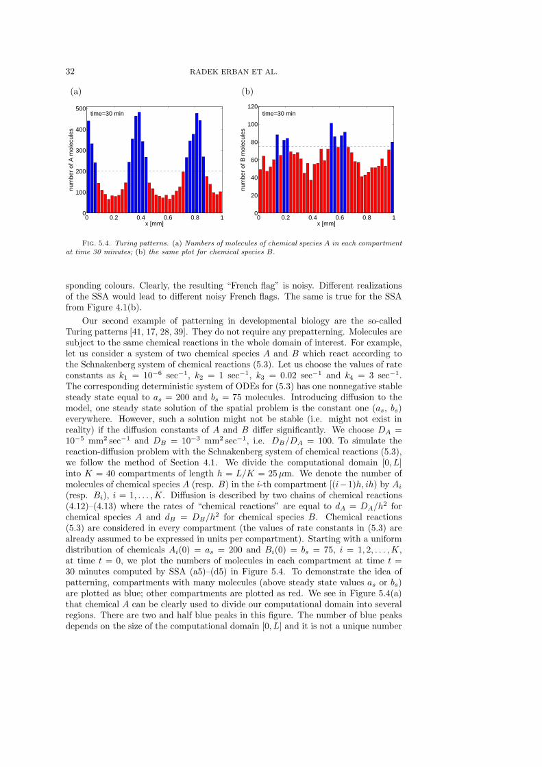
32 RADEK ERBAN ET AL.
(a)
0 0.2 0.4 0.6 0.8 10
100
200
300
400
500
x [mm]
num
ber
of A
mol
ecul
es
time=30 min
(b)
0 0.2 0.4 0.6 0.8 10
20
40
60
80
100
120
x [mm]
num
ber
of B
mol
ecul
es
time=30 min
Fig. 5.4. Turing patterns. (a) Numbers of molecules of chemical species A in each compartmentat time 30 minutes; (b) the same plot for chemical species B.
sponding colours. Clearly, the resulting “French flag” is noisy. Different realizationsof the SSA would lead to different noisy French flags. The same is true for the SSAfrom Figure 4.1(b).
Our second example of patterning in developmental biology are the so-calledTuring patterns [41, 17, 28, 39]. They do not require any prepatterning. Molecules aresubject to the same chemical reactions in the whole domain of interest. For example,let us consider a system of two chemical species A and B which react according tothe Schnakenberg system of chemical reactions (5.3). Let us choose the values of rateconstants as k1 = 10−6 sec−1, k2 = 1 sec−1, k3 = 0.02 sec−1 and k4 = 3 sec−1.The corresponding deterministic system of ODEs for (5.3) has one nonnegative stablesteady state equal to as = 200 and bs = 75 molecules. Introducing diffusion to themodel, one steady state solution of the spatial problem is the constant one (as, bs)everywhere. However, such a solution might not be stable (i.e. might not exist inreality) if the diffusion constants of A and B differ significantly. We choose DA =10−5 mm2 sec−1 and DB = 10−3 mm2 sec−1, i.e. DB/DA = 100. To simulate thereaction-diffusion problem with the Schnakenberg system of chemical reactions (5.3),we follow the method of Section 4.1. We divide the computational domain [0, L]into K = 40 compartments of length h = L/K = 25µm. We denote the number ofmolecules of chemical species A (resp. B) in the i-th compartment [(i−1)h, ih) by Ai
(resp. Bi), i = 1, . . . ,K. Diffusion is described by two chains of chemical reactions(4.12)–(4.13) where the rates of “chemical reactions” are equal to dA = DA/h2 forchemical species A and dB = DB/h2 for chemical species B. Chemical reactions(5.3) are considered in every compartment (the values of rate constants in (5.3) arealready assumed to be expressed in units per compartment). Starting with a uniformdistribution of chemicals Ai(0) = as = 200 and Bi(0) = bs = 75, i = 1, 2, . . . ,K,at time t = 0, we plot the numbers of molecules in each compartment at time t =30 minutes computed by SSA (a5)–(d5) in Figure 5.4. To demonstrate the idea ofpatterning, compartments with many molecules (above steady state values as or bs)are plotted as blue; other compartments are plotted as red. We see in Figure 5.4(a)that chemical A can be clearly used to divide our computational domain into severalregions. There are two and half blue peaks in this figure. The number of blue peaksdepends on the size of the computational domain [0, L] and it is not a unique number

STOCHASTIC REACTION-DIFFUSION PROCESSES 33
in general. The reaction-diffusion system has several favourable states with a differentnumber of blue peaks. As discussed in Section 5.1, the solution of the correspondingdeterministic model converges to one of the favourable (stable steady) states of thesystem. The stochastic model enables stochastic switching between the favourablestates, i.e. between the states with a different number of blue peaks.
6. Discussion. We presented SSAs for systems of chemical reactions and molec-ular diffusion. Then we presented methods for simulating both reactions and diffusionat the same time. The algorithms for simulating (spatially homogeneous) systems ofchemical reactions were based on the work of Gillespie [18]. We did not focus on thecomputer implementation of the algorithms. We chose simple examples which canbe simulated quickly. If one considers systems of many equations, there are waysto make the Gillespie SSA more efficient [16]. For example, it would be a waste oftime to recompute all the propensity functions at each time step. We simulate onereaction per one time step. Therefore, it makes sense to update only those propensityfunctions which are changed by the chemical reaction which was selected in step (d5)of SSA (a5)–(d5).
We only briefly touched on the concept of the Fokker-Planck equation [34] whenwe discussed the Smoluchowski description of diffusion. It is worth noting that thereare interesting connections between the chemical master equation (which is equivalentto the Gillespie SSA) and the Fokker-Planck equation which gives the time evolutionof the probability distribution. Such connections are discussed (through the so-calledchemical Langevin equation) in [20]. The Smoluchowski equation is actually the samemathematical object as the chemical Langevin equation, i.e. the stochastic differentialequation [2]. An algorithmic introduction to stochastic differential equations can befound in [23].
We presented two models of diffusion in this paper. One was based on the chain of“chemical reactions” (3.8) computing the time evolution of the numbers of moleculesin compartments. Coupling this model with the modelling of chemical reactions isstraightforward and presented in Section 4.1; such a compartment-based approachis used e.g. in [40, 24, 22]. The second model for molecular diffusion was based onthe Smoluchowski equation (3.6). It was an example of the so-called position jumpprocess, that is, a molecule jumps to a different location at each time step. As a result,the trajectory of a molecule is discontinuous. The individual trajectories of diffusingmolecules can be also modelled using the so-called velocity jump processes [29], thatis, the position of a molecule x(t) follows the deterministic equation dx/dt = v wherev(t), the velocity of the molecule, changes stochastically. Such stochastic processes canbe used not only for the simulation of diffusing molecules but also for the descriptionof movement of unicellular organisms like bacteria [10, 11] or amoeboid cells [12].Velocity jump processes can be also described in terms of PDEs for the time evolutionof the probability distributions to find a particle (molecule or cell) at a given place.Such equations are not exactly equal to the diffusion equation. However, they can bereduced in the appropriate limit to the diffusion equation [43, 7]. A classical reviewpaper on diffusion and other stochastic processes was written by Chandrasekhar [4],a nice introduction to random walks in biology is the book by Berg [3].
In this paper, we used only reflective boundary conditions, that is, particles hittingthe boundary were reflected back. Such boundary conditions are suitable wheneverthere is no chemical interaction between molecules in the solution and the boundaryof the domain. Considering biological applications, it is often the case that molecules(e.g. proteins) react with the boundary (e.g. with receptors in the cellular mem-

34 RADEK ERBAN ET AL.
brane). Then the boundary conditions have to be modified accordingly. It has to beassumed that some molecules which hit the boundary are reflected and some moleculesare adsorbed by the boundary (e.g. become bound to the receptor or take part inmembrane-based chemical reactions). The probability that a molecule is adsorbedrather than reflected depends on the chemical properties of the boundary and also onthe SSA which is used for modelling (further details are given in [7, 8]).
Our analysis of SSAs was based on the chemical master equation. We successfullyderived equations for the means and variances in illustrative examples which didnot include second-order reactions. Other first-order reaction networks can be alsoanalysed using this framework [13]. The nonlinear chemical kinetics complicates themathematical analysis significantly. We can write a deterministic description but itmight be too far from the correct description of the system [35]. A review of morecomputational approaches for the analysis of SSAs can be found in [26]. Applicationsof such methods to stochastic reaction-diffusion processes is presented in [31].
Acknowledgements. This work was supported by the Biotechnology and Bi-ological Sciences Research Council (grant ref. BB/C508618/1), St. John’s College,Oxford and Linacre College, Oxford (RE). Authors would like to give thanks for help-ful suggestions and encouraging comments during the preparation of this manuscriptto Ruth Baker, Hyung Ju Hwang, Chang Hyeong Lee, Hans Othmer, Jan Rychtarand Aidan Twomey.
REFERENCES
[1] S. Andrews and D. Bray, Stochastic simulation of chemical reactions with spatial resolutionand single molecule detail, Physical Biology 1 (2004), 137–151.
[2] L. Arnold, Stochastic Differential Equations, theory and applications, Wiley-Interscience Pub-lication, 1974.
[3] H. Berg, Random Walks in Biology, Princeton University Press, 1983.[4] S. Chandrasekhar, Stochastic problems in physics and astronomy, Reviews of Modern Physics
15 (1943), 2–89.[5] R. DeVille, C. Muratov, and E. Vanden-Eijnden, Non-meanfield deterministic limits in chem-
ical reaction kinetics, Journal of Chemical Physics 124 (2006), 231102.[6] M. Elowitz, A. Levine, E. Siggia, and P. Swain, Stochastic gene expression in a single cell,
Science 297 (2002), 1183–1186.[7] R. Erban and S. J. Chapman, Reactive boundary conditions for stochastic simulations of
reaction-diffusion processes, Physical Biology 4 (2007), no. 1, 16–28.[8] , Time scale of random sequential adsorption, Physical Review E 75 (2007), no. 4,
041116.[9] R. Erban, I. Kevrekidis, D. Adalsteinsson, and T. Elston, Gene regulatory networks: A coarse-
grained, equation-free approach to multiscale computation, Journal of Chemical Physics124 (2006), 084106.
[10] R. Erban and H. Othmer, From individual to collective behaviour in bacterial chemotaxis,SIAM Journal on Applied Mathematics 65 (2004), no. 2, 361–391.
[11] , From signal transduction to spatial pattern formation in E. coli: A paradigm for multi-scale modeling in biology, Multiscale Modeling and Simulation 3 (2005), no. 2, 362–394.
[12] , Taxis equations for amoeboid cells, Journal of Mathematical Biology 54 (2007), no. 6,847–885.
[13] C. Gadgil, C. Lee, and H. Othmer, A stochastic analysis of first-order reaction networks,Bulletin of Mathematical Biology 67 (2005), 901–946.
[14] G.W. Gardiner, Handbook of Stochastic Processes for physics, chemistry and natural sciences,2 ed., Springer Verlag, 1985.
[15] T. Gardner, C. Cantor, and J. Collins, Construction of a genetic toggle switch in E. coli, Nature403 (2000), 339–342.
[16] M. Gibson and J. Bruck, Efficient exact stochastic simulation of chemical systems with manyspecies and many channels, Journal of Physical Chemistry A 104 (2000), 1876–1889.
STOCHASTIC REACTION-DIFFUSION PROCESSES 35
[17] A. Gierer and H. Meinhardt, A theory of biological pattern formation, Kybernetik 12 (1972),30–39.
[18] D. Gillespie, Exact stochastic simulation of coupled chemical reactions, Journal of PhysicalChemistry 81 (1977), no. 25, 2340–2361.
[19] , Markov Processes, an introduction for physical scientists, Academic Press, Inc., Har-court Brace Jovanowich, 1992.
[20] , The chemical Langevin equation, Journal of Chemical Physics 113 (2000), no. 1, 297–306.
[21] J. Hasty, D. McMillen, and J. Collins, Engineered gene circuits, Nature 420 (2002), 224–230.[22] J. Hattne, D. Fange, and J. Elf, Stochastic reaction-diffusion simulation with MesoRD,
Bioinformatics 21 (2005), no. 12, 2923–2924.[23] D.J. Higham, An algorithmic introduction to numerical simulation of stochastic differential
equations, SIAM Review 43 (2001), no. 3, 525–546.[24] S. Isaacson and C. Peskin, Incorporating diffusion in complex geometries into stochastic chem-
ical kinetics simulations, SIAM Journal on Scientific Computing 28 (2006), no. 1, 47–74.[25] T. Kepler and T. Elston, Stochasticity in transcriptional regulation: Origins, consequences and
mathematical representations, Biophysical Journal 81 (2001), 3116–3136.[26] I. Kevrekidis, C. Gear, J. Hyman, P. Kevrekidis, O. Runborg, and K. Theodoropoulos,
Equation-free, coarse-grained multiscale computation: enabling microscopic simulators toperform system-level analysis, Communications in Mathematical Sciences 1 (2003), no. 4,715–762.
[27] C. Muratov, E. Vanden-Eijnden, and W. E, Self-induced stochastic resonance in excitablesystems, Physica D 210 (2005), 227–240.
[28] J. Murray, Mathematical Biology, Springer Verlag, 2002.[29] H. Othmer, S. Dunbar, and W Alt, Models of dispersal in biological systems, Journal of Math-
ematical Biology 26 (1988), 263–298.[30] J. Paulsson, O. Berg, and M. Ehrenberg, Stochastic focusing: Fluctuation-enhanced sensitivity
of intracellular regulation, Proceedings of the National Academy of Sciences USA 97 (2000),no. 13, 7148–7153.
[31] L. Qiao, R. Erban, C. Kelley, and I. Kevrekidis, Spatially distributed stochastic systems:Equation-free and equation-assisted preconditioned computation, Journal of ChemicalPhysics 125 (2006), 204108.
[32] C. Rao, D. Wolf, and A. Arkin, Control, exploitation and tolerance of intracellular noise,Nature 420 (2002), 231–237.
[33] G. Reeves, R. Kalifa, D. Klein, M. Lemmon, and S. Shvartsmann, Computational analysis ofEGFR inhibition by Argos, Developmental biology 284 (2005), 523–535.
[34] H. Risken, The Fokker-Planck Equation, methods of solution and applications, Springer-Verlag,1989.
[35] M. Samoilov and A. Arkin, Deviant effects in molecular reaction pathways, Nature Biotechnol-ogy 24 (2006), no. 10, 1235–1240.
[36] F. Schlogl, Chemical reaction models for non-equilibrium phase transitions, Zeitschrift furPhysik 253 (1972), no. 2, 147–161.
[37] J. Schnakenberg, Simple chemical reaction systems with limit cycle behaviour, Journal of The-oretical Biology 81 (1979), 389–400.
[38] O. Shimmi, D. Umulis, H. Othmer, and M. Connor, Faciliated transport of a Dpp/Scw het-erodimer by Sog/Tsg leads to robust patterning of the Drosophila blastoderm embryo, Cell120 (2005), no. 6, 873–886.
[39] S. Sick, S. Reinker, J. Timmer, and T. Schlake, WNT and DKK determine hair follicle spacingthrough a reaction-diffusion mechanism, Science 314 (2006), 1447–1450.
[40] A. Stundzia and C. Lumsden, Stochastic simulation of coupled reaction-diffusion processes,Journal of Computational Physics 127 (1996), 196–207.
[41] A. Turing, The chemical basis of morphogenesis, Phil. Trans. Roy. Soc. Lond. 237 (1952),37–72.
[42] L. Wolpert, R. Beddington, T. Jessel, P. Lawrence, E. Meyerowitz, and J. Smith, Principles ofDevelopment, Oxford University Press, 2002.
[43] E. Zauderer, Partial Differential Equations of Applied Mathematics, John Wiley & Sons, 1983.