a polynomial-space exact algorithm for tsp in … · a polynomial-space exact algorithm for tsp in...

A POLYNOMIAL-SPACE EXACT ALGORITHM FOR

TSP IN DEGREE-5 GRAPHS

Norhazwani Md Yunos1,2, Aleksandar Shurbevski1, Hiroshi Nagamochi1

1Department of Applied Mathematics and Physics, Graduate School of Informatics, KyotoUniversity, 606-8177, Kyoto, Japan

2Universiti Teknikal Malaysia Melaka, 76100 Durian Tunggal, Melaka, Malaysia{wanie, shurbevski, nag}@amp.i.kyoto-u.ac.jp

Keywords: Traveling Salesman Problem, Exact Ex-ponential Algorithm, Branch-and-reduce, Measure-and-conquer.

Abstract

The Traveling Salesman Problem (TSP) is one of themost well-known NP-hard optimization problems. Fol-lowing a recent trend of research which focuses on de-veloping algorithms for special types of TSP instances,namely graphs of limited degree, and thus alleviatinga part of the time and space complexity, we present apolynomial-space branching algorithm for the TSP ingraphs with degree at most 5, and show that it hasa running time of O∗(2.4723n). To the best of ourknowledge, this is the first exact algorithm specializedto graphs of such high degree. While the base of theexponent in the running time bound is greater thantwo, our algorithm uses space merely polynomial in aninput instance size, and thus by far outperforms Gure-vich and Shelah’s O∗(4nnlogn) polynomial-space exactalgorithm for the general TSP (Siam Journal of Com-putation, Vol. 16, No. 3, pp. 486-502, 1987). In theanalysis of the running time, we use the measure-and-conquer method, and we develop a set of branchingrules which foster the analysis of the running time.

1 Introduction

The Traveling Salesman Problem (TSP) is one of themost extensively studied problems in optimization. Ithas been formulated as a mathematical problem in the1930s. Many algorithmic methods have been investi-gated to beat the challenge of finding the fastest algo-rithm in terms of running time. On the other hand, ithas proven even more challenging to devise fast algo-rithms that would use a manageable amount of com-putation space, bounded by a polynomial in an inputinstance’s size. We will review previous algorithmicattempts, making a distinction between those whichrequire space exponential in the size of a problem in-stance, and those requiring space merely polynomialin the input size. We use the O∗ notation, which sup-presses polynomial factors.

The first non-trivial algorithm for the TSP in an n-vertex graph is the O∗(2n)-time dynamic programmingalgorithm discovered independently by Bellman [1],

and Held and Karp [9] in the early 1960s. This dy-namic programming algorithm however, requires alsoan exponential amount of space. Ever since, this run-ning time has only been improved for special types ofgraphs. Primarily, investigation efforts have been fo-cused on graphs in which vertices have a limited de-gree. Henceforth, let degree-i graph stand for a graphin which vertices have maximum degree at most i. Arecent improvement of the time bound to O∗(1.2186n)for degree-3 graphs has been presented by Bodlaen-der et al. [2]. They have used a general approach forspeeding up straightforward dynamic programming al-gorithms. For TSP in degree-4 graphs, Gebauer [7] hasshown a time bound of O∗(1.733n), by using a dynamicprogramming approach.

In the vein of polynomial space algorithms, Gure-vich and Shelah [8] have shown that the TSP in a gen-eral n-vertex graph is solvable in time O∗

(4nnlogn

).

Eppstein [4] has started the exploration into polyno-mial space TSP algorithms specialized for graphs ofbounded degree by designing an algorithm for degree-3graphs that runs in O∗(1.260n)-time. He introduceda branch-and-search method by considering a gener-alization of the TSP called the forced TSP. Iwamaand Nakashima [10] have claimed an improvement ofEppstein’s time bound to O∗(1.251n)-time for TSPin degree-3 graphs. Later, Liskiewicz and Schus-ter [11] have uncovered some oversights made in Iwamaand Nakashima’s analysis, and proved that their al-gorithm actually runs in O∗(1.257n)-time. Liskiewiczand Schuster then made some minor modificationsof Eppstein’s algorithm and showed that this modi-fied algorithm runs in O∗(1.2553n)-time, a slight im-provement over Iwama and Nakashima’s algorithm.Xiao and Nagamochi [14] have recently presentedan O∗(1.2312n)-time algorithm for TSP in degree-3graphs, and this improved previous time bounds forpolynomial-space algorithms. They used the basicsteps of Eppstein’s branch-and-search algorithm, andintroduced a branching rule based on a cut-circuitstructure. In the process of improving the time bound,they used simple analysis of measure and conquer, andeffectively analyzed their algorithm by introducing anamortization scheme over the cut circuit structure, set-ting weights to both vertices and connected compo-

2015 ISORA 978-1-78561-086-8 ©2015 IET 45 Luoyang, China, August 21–24, 2015

nents of induced graphs.

For TSP in degree-4 graphs, Eppstein [4] designedan algorithm that runs in O∗(1.890n)-time, based ona branch-and-search method. Later, Xiao and Nag-amochi [13] showed an improved value for the upperbound of the running time and showed that their algo-rithm runs in O∗(1.692n)-time. Currently, this is thefastest algorithm for TSP in degree-4 graphs. Basically,the idea behind their algorithm is to apply reductionrules until no further reduction is possible, and thenbranch on an edge by either including it to a solu-tion or excluding it from a solution. This is similarto most previous branch-and-search algorithms for theTSP. To effectively analyze their algorithm, Xiao andNagamochi used the measure and conquer method bysetting a weight to each vertex in a graph. From eachbranching operation, they derived a branching vec-tor using the assigned weight and evaluate how muchweight can be decreased in each of the two instancesobtained by branching on a selected edge e. In thisway, they were able to analyze by how much the to-tal weight would decrease in each branch. Moreover,they indicated that the measure will decrease more ifwe select a “good” edge to branch on, and gave a set ofsimple rules, based on a graph’s topological properties,for choosing such an edge. However, the analysis of therunning time itself is not as straightforward [13].

To the best of our knowledge, there exist no reportsin the literature of exact algorithms specialized to theTSP in degree-5 graphs. Therefore, this paper presentsthe first algorithm for the TSP in degree-5 graphs,and presents an upper bound on the running timeof O∗(2.4723n). In this exploration, we use a determin-istic branch-and-search algorithm for TSP in degree-5graphs. Basically, our algorithm employs similar tech-niques to most previous branching algorithms for theTSP. When there are no vertices of degree 5 in an in-put graph, we call an existing algorithm for TSP indegree-4 graphs, and solve the remaining instance. Inthe analysis, we use the measure and conquer methodas a tool to get an upper bound of the running time.

The remainder of this paper is organized as follows;Section 2 overviews the basic notation used in this pa-per and presents an introduction to the branching al-gorithm and measure and conquer method. Section3 describes our polynomial-space branching algorithm.We state our main result in section 4, where we proceedwith the analysis of the proposed algorithm. Finally,Section 5 concludes the paper.

2 Methods

2.1 Preliminaries

For a graph G, let V (G) denote the set of verticesin G, and let E(G) denote the set of edges in G.A pair of vertices v and u are called neighbors if vand u are adjacent by an edge uv. We denote theset of all neighbors of a vertex v by N(v), and de-

note by d(v) the cardinality |N(v)| of N(v), also calledthe degree of v. For a subset of vertices W ⊆ V (G),let N(v;W ) = N(v) ∩ W . For a subset of edgesE′ ⊆ E(G), let NE′(v) = N(v) ∩ {u | uv ∈ E′}, andlet dE′(v) = |NE′(v)|. Analogously, let NE′(v;W ) =NE′(v) ∩W , and dE′(v,W ) = |NE′(v,W )|. Also, fora subset E′ of E(G), we denote by G − E′ the graph(V,E \ E′) obtained from G by removing the edgesin E′.

We consider a generalization of the TSP, namedthe forced Traveling Salesman Problem. We define aninstance I = (G,F ) that consists of a simple, edgeweighted, undirected graph G, and a subset F of edgesin G, called forced. A vertex is called forced if exactlyone of its incident edges is forced. Similarly, it is calledunforced if no forced edge is incident to it. A Hamilto-nian cycle in G is called a tour if it passes through allthe forced edges in F . Under these circumstances, theforced TSP requests to find a minimum cost tour of aninstance (G,F ).

In this paper, we assume that the maximum degreeof a vertex in G is at most 5. We denote a forced(resp., unforced) vertex of degree i by fi (resp., ui).We are interested in six types of vertices in an instanceof (G,F ), namely, u5, f5, u4, f4, u3 and f3-vertices. Asshall be seen in Subsection 2.4.1, forced and unforcedvertices of degree 2 and 1 are treated as special cases.Let Vfi (resp., Vui), i = 3, 4, 5 denote the set of fi-vertices (resp., ui-vertices) in (G,F ).

2.2 Essentials on Branching Algorithms

We here review how to derive an upper bound on thenumber of instances that can be generated from aninitial instance by a branching algorithm.

We can represent the solution space in our branchingalgorithm as a search tree. This is a very useful way toillustrate the execution of the branching rules, and toaid the time analysis of the branching algorithm. Thesearch tree is obtained by assigning the input instanceof a problem as a root node, and recursively assigninga child to a node for each smaller instance obtainedby applying the branching rules. For a single node ofthe search tree, the algorithm takes time polynomial inthe size of the node instance, which in turn, is smallerthan or equal to the original instance size. Thus, wecan conclude that the running time of the branchingalgorithm is equal to the number of nodes of the searchtree times a polynomial of the original input instancesize.

Let I be a given instance with size µ, and let I ′ andI ′′ be instances obtained from I by a branching oper-ation. We use T (µ) to denote the maximum numberof nodes in the search tree of an input of size µ whenwe execute our branching algorithm. Let a and b bethe amounts of decrease in size of instances I ′ and I ′′,respectively; these values directly determine the per-formance of the algorithm. Then, we call (a, b) the


branching vector of the branching rules, and this im-plies the linear recurrence:

T (µ) ≤ T (µ− a) + T (µ− b) . (1)

To evaluate the performance of this branching vec-tor, we can use any standard method for linear recur-rence relations. In fact, it is known that T (µ) is of theform O (τµ), where τ is the unique positive real root ofthe function f(x) = 1−

(x−a + x−b

)[6]. The value τ is

called the branching factor (of a given branching vec-tor), and the running time of the algorithm decreaseswith the value of this branching factor.

2.3 The Measure-and-Conquer Method

To effectively analyze our search tree algorithm, we usethe measure and conquer method. A complete descrip-tion of this method is beyond the scope of this paper,and the interested reader might refer to the book ofFomin and Kratsch [6].

The basic idea behind the measure and conquermethod is to assign a measure to an instance, asopposed to using simply its size when analyzing thebranching vectors of the branching operations. A goodchoice for a measure might lead to a significantly im-proved analysis on the upper bound of the runningtime of a branching algorithm. For example, Fominet al. [5] have presented simple polynomial-space al-gorithms for the Maximum Independent Set and theMinimum Dominating Set Problem, and obtained animpressive refinement of the time analysis by using themeasure and conquer method. This shows that a goodchoice of measure is very important to the time boundsachievable.

For a given problem instance I of size µ, let W (I) bethe measure of I. When considering a branch and re-duce algorithm for the concerned problem, intuitivelywe seek for a measure which satisfies the followingproperties

(i) W (I) = 0 if and only if I can be solved in polyno-mial time;

(ii) If I ′ is a sub-instance of I obtained through a re-duction or a branching operation, then W (I ′) ≤W (I).

We call a measure W satisfying conditions (i) and (ii)above a proper measure.

2.4 A Polynomial-Space Branching Algo-rithm

We assume that the maximum degree of a vertex in agiven graph G is at most 5. Basically, our algorithmcontains two major steps. In the first step, the algo-rithm applies reduction rules until no further reductionis possible. In the second step, the algorithm appliesbranching rules in a reduced instance to search for asolution. These two steps are repeated iteratively.

As a result of the reduction and branching opera-tions, the degree of some vertices will decrease, whilethe degree of other vertices will remain unchanged. Aforced edge will never disappear, neither by the reduc-tion nor branching operations, but an unforced edgemay be erased by either of the reduction or branchingoperation. Throughout the process of the reductionand branching operations, the measure of an instancewill never increase.

Details about the reduction and branching proce-dures will be discussed in the following sub-sections.

2.4.1 Reduction Rules

Reduction is a process of transforming an instance toa smaller instance. It takes polynomial-time to obtaina solution of an original instance from a solution of asmaller instance that has been obtained by a reductionprocedure from the original instance.

Not all forced TSP instances have a tour. If an in-stance has no tour, we called it infeasible. Lemma 1gives two sufficient conditions for an instance to be in-feasible.

Lemma 1 If one of the following conditions holds,then the instance (G,F ) is infeasible.

(i) d(v) ≤ 1 for some vertex v ∈ V (G).(ii) dF(v) ≥ 3 for some vertex v ∈ V (G).

In this paper, there are two reduction rules appliedin each of the branching operation. These reductionrules preserve the minimum cost tour of an instance,as stated in Lemma 2.

Lemma 2 Each of the following reductions preservesthe feasibility and a minimum cost tour of an in-stance (G,F ).

(i) If d(v) = 2 for a vertex v, then add to F anyunforced edge incident to vertex v; and

(ii) If d(v) > 2 and dF(v) = 2 for a vertex v, thenremove from G any unforced edge incident to ver-tex v.

Proof. Statements (i) and (ii) immediately follow fromthe definition of tours. �

From Lemma 1 and Lemma 2, we form our reductionalgorithm as described in Figure 1. An instance (G,F )which does not satisfy any of the conditions in Lemma 1and Lemma 2 is called reduced.

2.4.2 Branching Rules

Our algorithm iteratively branches on an unforced edgee in a reduced instance I = (G,F ) by either including einto F , force(e), or excluding it from G, delete(e). Byapplying a branching operation, the algorithm gener-ates two new instances, called branches, by adding anunforced edge to F , or by removing it from G.


Input: An instance (G,F ) such that the maximumdegree of G is at most 5.Output: A message for the infeasibility of (G,F ); or areduced instance (G′, F ′) of (G,F ).

Initialize (G′, F ′) := (G,F );

while (G′, F ′) is not a reduced instance do

If there is a vertex v in (G′, F ′) such that d(v) ≤ 1or dF ′(v) ≥ 3 then

Return message “Infeasible”

Elseif there is a vertex v in (G′, F ′) such that 2 =d(v) > dF ′(v) then

Let E† be the set of unforced edges incident to allsuch vertices;Set F ′ := F ′ ∪ E†

Elseif there is a vertex v in (G′, F ′) such that d(v) >dF ′(v) = 2 then

Let E† be the set of unforced edges incident to allsuch vertices;Set G′ := G′ − E†

End while;Return (G′, F ′).

Figure 1: Algorithm Red(G,F )

To describe our branching algorithm, let (G,F ) be areduced instance such that the maximum degree of G isat most 5. In (G,F ), an unforced edge e = vt incidentto a vertex v of degree 5 is called optimal, if it satisfiesa condition (c-i) below with minimum index i, over allunforced edges vt in (G,F ):

(c-1) v ∈ Vf5 and t ∈ NU (v;Vf3) such that NU (v) ∩NU (t) = ∅;

(c-2) v ∈ Vf5 and t ∈ NU (v;Vf3) such that NU (v) ∩NU (t) 6= ∅;

(c-3) v ∈ Vf5 and t ∈ NU (v;Vu3);(c-4) v ∈ Vf5 and t ∈ NU (v;Vf4) such that NU (v) ∩

NU (t) = ∅;(c-5) v ∈ Vf5 and t ∈ NU (v;Vf4) such that NU (v) ∩

NU (t) 6= ∅;(I) |NU (v) ∩NU (t)| = 1; and

(II) |NU (v) ∩NU (t)| = 2;(c-6) v ∈ Vf5 and t ∈ NU (v;Vu4);(c-7) v ∈ Vf5 and t ∈ NU (v;Vf5) such that NU (v) ∩

NU (t) = ∅;(c-8) v ∈ Vf5 and t ∈ NU (v;Vf5) such that NU (v) ∩

NU (t) 6= ∅;(I) |NU (v) ∩NU (t)| = 1;

(II) |NU (v) ∩NU (t)| = 2; and(III) |NU (v) ∩NU (t)| = 3;

(c-9) v ∈ Vf5 and t ∈ NU (v;Vu5);(c-10) v ∈ Vu5 and t ∈ NU (v;Vf3);(c-11) v ∈ Vu5 and t ∈ NU (v;Vf4);(c-12) v ∈ Vu5 and t ∈ NU (v;Vu3);(c-13) v ∈ Vu5 and t ∈ NU (v;Vu4); and(c-14) v ∈ Vu5 and t ∈ NU (v;Vu5).

We refer to the above conditions for choosing an op-timal edge to branch on, c-1 to c-14, as the branchingrules. The collective set of branching rules are illus-trated in Figure 2.

For convenience in the analysis of the algorithm, case(c-5) and case (c-8) have been subdivided into subcasesaccording to the cardinality of the neighborhood inter-section. Intersections of lower cardinality take prece-dence over higher ones.

Given a reduced instance I = (G,F ), our algorithmfirst checks whether there exists a vertex of degree 5,and if it does, chooses an optimal edge according to thebranching rules. If there exists no optimal edge accord-ing to the branching rules, then the reduced instancehas no more vertices of degree 5, and the maximum de-gree of the reduced instance at this point is at most 4.Then, we can call a polynomial space exact algorithmfor the TSP that is specialized for degree-4 graphs, e.g.,the algorithm specialized for degree-4 graphs by Xiaoand Nagamochi [13]. Our branching algorithm is de-scribed in Figure 3.

2.4.3 Weight Setting

In order to obtain a measure which will imply the samerunning time bound as a function of the size of a TSPinstance, we require that the weight of each vertex isnot greater than 1. In what follows, we examine somenecessary constraints which the vertex weights shouldsatisfy in order to obtain a proper measure.

For i = {3, 4, 5}, we denote wi to be the weight ofa ui-vertex, and wi′ to be the weight of an fi-vertex.The conditions for a proper measure require that themeasure of an instance obtained through a branchingor a reduction operation will not be greater than themeasure of the original instance. Thus, vertex weightsshould satisfy the following relations

w5 ≤ 1, (2)

w5′ ≤ w5, (3)

w4′ ≤ w4, (4)

w3′ ≤ w3, (5)

w3 ≤ w4 ≤ w5, and (6)

w3′ ≤ w4′ ≤ w5′ . (7)

The vertex weight for vertices of degree less than 3 isset to be 0.

We proceed to show in the algorithms given in Fig-ures 1 and 3, setting vertex weights which satisfy theconditions of Eqs. (3) to (7) is sufficient to obtain aproper measure.

Lemma 3 If the weights of vertices are chosen as inEqs. (3) to (7), then the measure W (I) never increasesas a result of the reduction or the branching operationsof Figure 1 and Figure 3.

Proof. Let I = (G,F ) be a given instance of the forcedTSP. Due to our definition of the measure W (I) of


: unforced edges : forced edges

c-1

v

t1

t2 t3

t4

e

t5

c-2

v

t1

t2 t3

t4

e

c-3

v

t1

t2 t3

t4

e

t5 t6

c-4

v

t1

t2 t3

t4

e

t5 t6

c-5(I)

v

t1

t2 t3

t4

e

t5

c-5(II)

v

t1

t2 t3

t4

e

c-6

t7

v

t1

t2 t3

t4

e

t5 t6c-7

t7

v

t1

t2 t3

t4

e

t5 t6

c-8(I)

v

t1

t2 t3

t4

e

t5 t6

c-8(II)

v

t1

t2 t3

t4

e

t5

c-8(III)

v

t1

t2 t3

t4

e

c-9t7

v

t1

t2 t3

t4

e

t5 t6

t8

c-10

v

t1

t2

e

t6

t3

t4

t5

c-11

v

t1

t2

e

t6 t7

t3

t4

t5

c-12

v

t1

t2

e

t6 t7

t3

t4

t5

c-14

t3

t4

t5

t8

v

t1

t2

e

t6 t7

t9

c-13

t3

t4

t5

t8

v

t1

t2

e

t6 t7

Figure 2: Illustration of the Branching Rules

Eq.(18), it suffices to show that none of the individualvertex weights will increase as a result of a reductionor a branching operation in the algorithms of Figures 1

and 3.

The branching rules state that for an unforced edgee in E(G)\F , two subinstances are generated by either


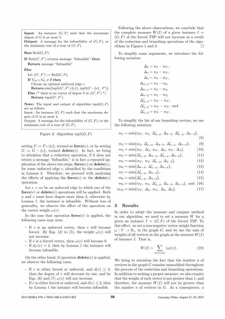
Input: An instance (G,F ) such that the maximumdegree of G is at most 5.Output: A message for the infeasibility of (G,F ); orthe minimum cost of a tour of (G,F ).

Run Red(G,F );

If Red(G′, F ′) returns message “Infeasible” then

Return message “Infeasible”

Else

Let (G′, F ′) := Red(G,F );

If Vu5 ∪ Vf5 6= ∅ thenChoose an optimal unforced edge eReturnmin{tsp5(G′, F ′∪{e}), tsp5(G′−{e}, F ′)}

Else /* there is no vertex of degree 5 in (G′, F ′) */Return tsp4(G′, F ′).

Note: The input and output of algorithm tsp4(G,F )are as followsInput: An instance (G,F ) such that the maximum de-gree of G is at most 4.Output: A message for the infeasibility of (G,F ); or theminimum cost of a tour of (G,F ).

Figure 3: Algorithm tsp5(G,F )

setting F := F ∪{e}, termed as force(e), or by settingG := G − {e}, termed delete(e). In fact, we bringto attention that a reduction operation, if it does notreturn a message “Infeasible,” is in fact a repeated ap-plication of the above two steps, force(e) or delete(e),for some unforced edge e, identified by the conditionsin Lemma 2. Therefore, we proceed with analyzingthe effects of applying the force(e) or the delete(e)operation.

Let e = uv be an unforced edge to which one of theforce(e) or delete(e) operations will be applied. Bothu and v must have degree more than 2, otherwise byLemma 1, the instance is infeasible. Without loss ofgenerality, we observe the effect of the operation onthe vertex weight ω(v).

In the case that operation force(e) is applied, thefollowing cases may arise.

− If v is an unforced vertex, then v will becomeforced. By Eqs. (3) to (5), the weight ω(v) willnot increase.

− If v is a forced vertex, then ω(v) will become 0.− If dF (v) = 2, then by Lemma 1 the instance will

become infeasible.

On the other hand, if operation delete(e) is applied,we observe the following cases.

− If v is either forced or unforced, and d(v) ≥ 3,then the degree of v will decrease by one, and byEqs. (6) and (7) ω(v) will not increase.

− If v is either forced or unforced, and d(v) ≤ 2, thenby Lemma 1 the instance will become infeasible.

Following the above observations, we conclude thatthe complete measure W (I) of a given instance I =(G,F ) of the forced TSP will not increase as a resultof the reduction and branching operations of the algo-rithms in Figures 1 and 3. �

To simplify some arguments, we introduce the fol-lowing notation:

∆3 = w3 − w3′ ,

∆4 = w4 − w4′ ,

∆5 = w5 − w5′ ,

∆4−3 = w4 − w3,

∆5−4 = w5 − w4,

∆5−3 = w5 − w3,

∆′4−3 = w4′ − w3′ ,

∆′5−4 = w5′ − w4′ , and

∆′5−3 = w5′ − w3′ .

To simplify the list of our branching vectors, we usethe following notation:

m1 = min{w3′ , w3, ∆′4−3, ∆4−3, ∆′5−4, ∆5−4},(8)

m2 = min{w3, ∆′4−3, ∆4−3, ∆′5−4, ∆5−4}, (9)

m3 = min{w3′ , ∆3, w4′ , ∆4, w5′ , ∆5}, (10)

m4 = min{∆′4−3, ∆4−3, ∆′5−4, ∆5−4}, (11)

m5 = min{w4′ , w4, ∆′5−3, ∆5−3}, (12)

m6 = min{∆4−3, ∆′5−4, ∆5−4}, (13)

m7 = min{∆′5−4, ∆5−4}, (14)

m8 = min{∆′5−3, ∆5−3}, (15)

m9 = min{w3′ , w3, ∆′4−3, ∆4−3, ∆5−4}, and (16)

m10 = min{w3′ , ∆3, w4′ , ∆4, ∆5}. (17)

3 Results

In order to adopt the measure and conquer methodin our algorithm, we need to set a measure W for agiven an instance I = (G,F ) of the forced TSP. Tothis effect, we set a non-negative vertex weight functionω : V → R+ in the graph G, and we use the sum ofweights of all vertices in the graph as the measure W (I)of instance I. That is,

W (I) =∑

v∈V (G)

(ω(v)) . (18)

We bring to attention the fact that the number n ofvertices in the graph G remains unmodified throughoutthe process of the reduction and branching operations.In addition to seeking a proper measure, we also requirethat the weight of each vertex is not greater than 1, andtherefore, the measure W (I) will not be greater thanthe number n of vertices in G. As a consequence, a


running time bound as a function of the measure W (I)implies the same running time bound as a functionof n. The weight assigned to each vertex type plays animportant role, since the value of the branching factordepends solely on these weights.

Let the vertex weight function ω(v) be chosen asfollows:

ω(v) =

w3′ = 0.183471 for an f3-vertex v

w3 = 0.322196 for a u3-vertex v


w4 = 0.700651 for a u4-vertex v


w5 = 1 for a u5-vertex v

0 otherwise.

(19)

Lemma 4 If the vertex weight function ω(v) is set asin Eq. (19), then each branching operation in Figure 3has a branching factor not greater than 2.472232.

A proof of Lemma 4 will be derived analytically inthe several subsections which follow. From the lemma,we get our main result:

Theorem 1 The TSP in an n-vertex graph G withmaximum degree 5 can be solved in O∗(2.4723n)-timeand polynomial-space.

In the remainder of the analysis, for an optimaledge e = vt1, we denote NU (v) by {t1, t2, . . . , ta},a = dU (v), and NU (t1) \ {v} by {ta+1, ta+1, . . . , ta+b},b = dU (t1) − 1. We assume without loss of gen-erality that t1+i = ta+i for i = 1, 2, . . . , c, wherec = |NU (v) ∩ NU (t1)|, the number of good neighborsthat v and t1 have in common.

3.1 Branching on Edges Around f5-vertices (c-1 to c-9)

This section derives branching vectors for the branch-ing operation on an optimal edge e = vt1, incident toan f5-vertex v, distinguishing nine cases for conditionsc-1 to c-9.

Case c-1: There exist vertices v ∈ Vf5 and t1 ∈NU (v;Vf3) such that NU (v) ∩ NU (t1) = ∅ (see Fig-ure 4): We branch on edge vt1. Note that NU (t1) \{v} = {t5}.

In the branch of force(vt1), edge vt1 will be addedto F ′ by the branching operation, and edges vt2,vt3, vt4 and t1t5 will be deleted from G′ by the re-duction rules. Both v and t1 will become verticesof degree 2. From Eq. (19), the weight of verticesof degree 2 is 0. So, the weight of vertex v de-creases by w5′ and the weight of vertex t1 decreasesby w3′ . Each of the vertices t2, t3 and t4 can beeither a type f3, u3, f4, u4, f5, or u5-vertex, andeach of their weights would decrease by at least m1 =min

{w3′ , w3,∆

′4−3,∆4−3,∆′5−4,∆5−4

}. If vertex t5 is


: newly deleted edges : newly forced edges

(a) force(vt1) in c-1

v

t1

t2 t3

t4

e

t5

(b) delete(vt1) in c-1

v

t1

t2 t3

t4

e

t5

Figure 4: Illustration of branching rule c-1, where ver-tex v ∈ Vf5 and vertex t1 ∈ NU (v;Vf3) such thatNU (v) ∩NU (t1) = ∅.

an f3-vertex (resp., u3, f4, u4, f5, or a u5-vertex), thenthe weight decrease α of vertex t5 would be w3′ (resp.,w3, ∆′4−3, ∆4−3, ∆′5−4, and ∆5−4). Thus, the totalweight decrease in the branch of force(vt1) is at least(w5′ + w3′ + 3m1 + α).

In the branch of delete(vt1), edge vt1 will be deletedfrom G′ by the branching operation, and edge t1t5 willbe added to F ′ by the reduction rules. The weight ofvertex v decreases by ∆′5−4 and the weight of vertex t1decreases by w3′ . If vertex t5 is an f3-vertex (resp., u3,f4, u4, f5, or a u5-vertex), then the weight decrease βof vertex t5 would be w3′ (resp., ∆3, w4′ , ∆4, w5′ , and∆5). Thus, the total weight decrease in the branch ofdelete(vt1) is at least (w5′ − w4′ + w3′ + β).

As a result, we get the following six branching vec-tors:

(w5′ + w3′ + 3m1 + α, w5′ − w4′ + w3′ + β) (20)

for (α, β) ∈ {(w3′ , w3′), (w3,∆3), (∆′4−3, w4′),(∆4−3,∆4), (∆′5−4, w5′), (∆5−4,∆5)}.

c-2. There exist vertices v ∈ Vf5 and t1 ∈ NU (v;Vf3)such that NU (v) ∩ NU (t1) = {t2} (see Figure 5): Webranch on edge vt1.

In the branch of force(vt1), edge vt1 will be addedto F ′ by the branching operation, and edges vt2,vt3, vt4 and t1t2 will be deleted from G′ by the re-duction rules. So, the weight of vertex v decreasesby w5′ , and the weight of vertex t1 decreases byw3′ . Each of the vertices t3 and t4 can be eithera type f3, u3, f4, u4, f5, or u5-vertex, and eachof their weights would decrease by at least m1 =min

{w3′ , w3,∆

′4−3,∆4−3,∆′5−4,∆5−4

}.

There are two possible cases for the vertex type ofvertex t2. First, let t2 be an f3 or u3-vertex. Afterperforming the branching operation, t2 would becomea vertex of degree 1. By Lemma 1, case (i), this isinfeasible, and the algorithm will return a message ofinfeasibility.


v

t1

t2 t3

t4

e

(a) force(vt1) in c-2 (b) delete(vt1) in c-2

v

t1

t2 t3

t4

e



Figure 5: Illustration of branching rule c-2, where ver-tex v ∈ Vf5 and vertex t1 ∈ NU (v;Vf3) such thatNU (v) ∩NU (t1) = {t2}.

Second, let t2 be an f4, u4, f5, or u5-vertex. If t2is an f4-vertex (resp., u4, f5, or a u5-vertex), then theweight decrease α of vertex t2 would be w4′ (resp., w4,∆′5−3, and ∆5−3). Thus, the total weight decrease inthe branch of force(vt1) is at least (w5′+w3′+2m1+α).

In the branch of delete(vt1), edge vt1 will be deletedfrom G′ by the branching operation, and edge t1t2 willbe added to F ′ by the reduction rules. So, the weightsof vertices v and t1 decrease by ∆′5−4 and w3′ , respec-tively. If vertex t2 is an f4-vertex (resp., u4, f5, ora u5-vertex), then the weight decrease β of vertex t2would be w4′ (resp., ∆4, w5′ , and ∆5). Thus, the totalweight decrease in the branch of delete(vt1) is at least(w5′ − w4′ + w3′ + β).

As a result, we get the following four branching vec-tors:

(w5′ + w3′ + 2m1 + α, w5′ − w4′ + w3′ + β) (21)

for (α, β) ∈ {(w4′ , w4′), (w4,∆4), (∆′5−3, w5′),(∆5−3,∆5)}.

c-3. There exist vertices v ∈ Vf5 and t1 ∈ NU (v;Vu3)(see Figure 6): We branch on edge vt1. Note thatNU (t1) \ {v} = {t5, t6}.

In the branch of force(vt1), edge vt1 will be addedto F ′ by the branching operation, and edges vt2, vt3and vt4 will be deleted from G′ by the reduction rules.So, the weights of vertices v and t1 decrease by w5′

and ∆3, respectively. Each of vertices t2, t3 andt4 can be either a type u3, f4, u4, f5, or u5-vertex,and each of their weights would decrease by at leastm2 = min

{w3,∆

′4−3,∆4−3,∆′5−4,∆5−4

}. Thus, the

total weight decrease in the branch of force(vt1) is atleast (w5′ + w3 − w3′ + 3m2).

In the branch of delete(vt1), edge vt1 will be deletedfrom G′ by the branching operation and edges t1t5 andt1t6 will be added to F ′ by the reduction rules. So, theweight of vertex v decreases by ∆′5−4 and the weight ofvertex t1 decreases by w3. Each of the vertices t5 andt6 can be either a type f3, u3, f4, u4, f5, or u5-vertex,

v

t1

t2 t3

t4

e

t5 t6


v

t1

t2 t3

t4

e

t5 t6



Figure 6: Illustration of branching rule c-3, where ver-tex v ∈ Vf5 and vertex t1 ∈ NU (v;Vu3).

and each of their weights would decrease by at leastm3 = min {w3′ ,∆3, w4′ ,∆4, w5′ ,∆5}. Thus, the totalweight decrease in the branch of delete(vt1) is at least(w5′ − w4′ + w3 + 2m3).

As a result, we get the following branching vector:

(w5′ + w3 − w3′ + 3m2, w5′ − w4′ + w3 + 2m3) .(22)

c-4. There exist vertices v ∈ Vf5 and t1 ∈ NU (v;Vf4)such that NU (v) ∩ NU (t1) = ∅ (see Figure 7): Webranch on edge vt1. Note that NU (t1) \ {v} = {t5, t6}.

v

t1

t2 t3

t4

e

t5 t6

(b) delete(vt1) in c-4(a) force(vt1) in c-4

v

t1

t2 t3

t4

e

t5 t6



Figure 7: Illustration of branching rule c-4, where ver-tex v ∈ Vf5 and vertex t1 ∈ NU (v;Vf4), such thatNU (v) ∩NU (t1) = ∅.

In the branch of force(vt1), edge vt1 will be addedto F ′ by the branching operation, and edges vt2,vt3, vt4, t1t5 and t1t6 will be deleted from G′ bythe reduction rules. So, the weight of vertex v de-creases by w5′ and the weight of vertex t1 decreasesby w4′ . Each of the vertices t2, t3 and t4 canbe either a type f4, u4, f5, or u5-vertex, and eachof their weights would decrease by at least m4 =min

{∆′4−3,∆4−3,∆′5−4,∆5−4

}. Each of vertices t5

and t6 can be either a type f3, u3, f4, u4, f5, or u5-vertex, and each of their weights would decrease by


at least m1 = min{w3′ , w3,∆

′4−3,∆4−3,∆′5−4,∆5−4

}.

Thus, the total decrease in the branch of force(vt1) isat least (w5′ + w4′ + 3m4 + 2m1).

In the branch of delete(vt1), edge vt1 will be deletedfrom G′ by the branching operation. So, the weight ofvertex v decreases by ∆′5−4 and the weight of vertex t1decreases by ∆′4−3. Thus, the total weight decrease inthe branch of delete(vt1) is at least (w5′ −w3′). As aresult, we get the following branching vector:

(w5′ + w4′ + 3m4 + 2m1, w5′ − w3′) . (23)

c-5. There exist vertices v ∈ Vf5 and t1 ∈ NU (v;Vf4)such that NU (v)∩NU (t1) 6= ∅. We distinguish two subcases, according to the cardinality of the intersectionNU (v) ∩ NU (t1), (c-5(I)), |NU (v) ∩NU (t1)| = 1, and(c-5(II)), |NU (v) ∩NU (t1)| = 2.

c-5(I). Without loss of generality, assume thatNU (v) ∩ NU (t1) = {t2} (see Figure 8): We branchon edge vt1. Note that NU (t1) \ {v} = {t5}.

v

t1

t2 t3

t4

e

t5

(a) force(vt1) in c-5(I) (b) delete(vt1) in c-5(I)

v

t1

t2 t3

t4

e

t5



Figure 8: Illustration of branching rule c-5(I), wherevertex v ∈ Vf5 and vertex t1 ∈ NU (v;Vf4), such thatNU (v) ∩NU (t1) = {t2}.

In the branch of force(vt1), edge vt1 will be addedto F ′ by the branching operation, and edges vt2,vt3, vt4, t1t2, and t1t5 will be deleted from G′ bythe reduction rules. So, the weight of vertex v de-creases by w5′ and the weight of vertex t1 decreasesby w4′ . Vertex t2 can be either a type f4, u4, f5, oru5-vertex, and its weight would decrease by at leastm5 = min

{w4′ , w4,∆

′5−3,∆5−3

}. Each of the ver-

tices t3 and t4 can be either a type f4, u4, f5, or u5-vertex, and each of their weights would decrease byat least m4 = min

{∆′4−3,∆4−3,∆′5−4,∆5−4

}. Ver-

tex t5 can be either a type f3, u3, f4, u4, f5, oru5-vertex, and its weight would decrease by at leastm1 = min

{w3′ , w3,∆

′4−3,∆4−3,∆′5−4,∆5−4

}. Thus,

the total weight decrease in the branch of force(vt1)is at least (w5′ + w4′ +m5 + 2m4 +m1).

In the branch of delete(vt1), edge vt1 will be deletedfrom G′ by the branching operation. So, the weight of

vertex v decreases by ∆′5−4, and the weight of vertex t1decreases by ∆′4−3. Thus, the total weight decrease inthe branch of delete(vt1) is at least (w5′ −w3′). As aresult, we get the following branching vector:

(w5′ + w4′ +m5 + 2m4 +m1, w5′ − w3′) . (24)

c-5(II). Without loss of generality, assume thatNU (v) ∩ NU (t1) = {t2, t3} (see Figure 9): We branchon edge vt1.

v

t1

t2 t3

t4

e

(a) force(vt1) in c-5(II) (b) delete(vt1) in c-5(II)

v

t1

t2 t3

t4

e



Figure 9: Illustration of branching rule c-5(II), wherevertex v ∈ Vf5 and vertex t1 ∈ NU (v;Vf4) such thatNU (v) ∩NU (t1) = {t2, t3}.

In the branch of force(vt1), edge vt1 will be addedto F ′ by the branching operation, and edge vt2, vt3,vt4, t1t2 and t1t3 will be deleted from G′ by the re-duction rules. So, the weight of vertex v decreasesby w5′ and the weight of vertex t1 decreases by w4′ .Each of vertices t2 and t3 can be either a type f4, u4,f5, or u5-vertex, and each of their weights would de-crease by at least m5 = min

{w4′ , w4,∆

′5−3,∆5−3

}.

Vertex t4 can be either a type f3, u3, f4, u4, f5, oru5-vertex, and its weight would decreases by at leastm4 = min

{∆′4−3,∆4−3,∆′5−4,∆5−4

}. Thus, the total

weight decrease in the branch of force(vt1) is at least(w5′ + w4′ + 2m5 +m4).

In the branch of delete(vt1), edge vt1 will be deletedfrom G′ by the branching operation. So, the weight ofvertex v decreases by ∆′5−4, and the weight of vertex t1decreases by ∆′4−3. Thus, the total weight decrease inthe branch of delete(vt1) is at least (w5′ −w3′). As aresult, we get the following branching vector:

(w5′ + w4′ + 2m5 +m4, w5′ − w3′) . (25)

c-6. There exist vertices v ∈ Vf5 and t1 ∈ NU (v;Vu4)(see Figure 10): We branch on edge vt1. Note thatNU (t1) \ {v} = {t5, t6, t7}.

In the branch of force(vt1), edge vt1 will be addedto F ′ by the branching operation, and edges vt2, vt3and vt4 will be deleted from G′ by the reduction rules.So, the weight of vertex v decreases by w5′ and theweight of vertex t1 decreases by ∆4. Each of the ver-tices t2, t3 and t4 can be either a type u4, f5, or u5-vertex, and each of their weights would decrease by at


t7

v

t1

t2 t3

t4

e

t5 t6


t7

v

t1

t2 t3

t4

e

t5 t6



Figure 10: Illustration of branching rule c-6, wherevertex v ∈ Vf5 and vertex t1 ∈ NU (v;Vu4).

least m6 = min{

∆4−3,∆′5−4,∆5−4}

. Thus, the totalweight decrease in the branch of force(vt1) is at least(w5′ + w4 − w4′ + 3m6).

In the branch of delete(vt1), edge vt1 will be deletedfrom G′ by the branching operation. So, the weight ofvertex v decreases by ∆′5−4 and the weight of vertex t1decreases by ∆4−3. Thus, the total weight decrease inthe branch of delete(vt1) is at least (w5′ −w4′ +w4−w3). As a result, we get the following branching vector:

(w5′ + w4 − w4′ + 3m6, w5′ − w4′ + w4 − w3) . (26)

c-7. There exist vertices v ∈ Vf5 and t1 ∈ NU (v;Vf5)such that NU (v) ∩ NU (t1) = ∅ (see Figure 11): Webranch on edge vt1. Note that NU (t1) \ {v} ={t5, t6, t7}.

t7

v

t1

t2 t3

t4

e

t5 t6


t7

v

t1

t2 t3

t4

e

t5 t6



Figure 11: Illustration of branching rule c-7, wherevertex v ∈ Vf5 and vertex t1 ∈ NU (v;Vf5), such thatNU (v) ∩NU (t1) = ∅.

In the branch of force(vt1), edge vt1 will be addedto F ′ by the branching operation, and edges vt2, vt3,vt4, t1t5, t1t6 and t1t7 will be deleted from G′ by thereduction rules. So, both weights of vertex v and ver-tex t1 decreases by w5′ , each. Each of vertices t2,t3, t4, t5, t6 and t7 can be either a type f5, or u5-vertex, and each of their weights would decrease by

at least m7 = min{

∆′5−4,∆5−4}

. Thus, the totalweight decrease in the branch of force(vt1) is at least(2w5′ + 6m7).

In the branch of delete(vt1), edge vt1 will be deletedfrom G′ by the branching operation. So, both weightsof vertices v and t1 decreases by ∆′5−4, each. Thus, thetotal weight decrease in the branch of delete(vt1) isat least (2w5′−2w4′). As a result, we get the followingbranching vector:

(2w5′ + 6m7, 2w5′ − 2w4′) . (27)

c-8. There exist vertices v ∈ Vf5 and t1 ∈ NU (v;Vf5)such that NU (v) ∩ NU (t1) 6= ∅. We distinguish threesub cases, according to the cardinality of the inter-section NU (v) ∩NU (t1), (c-8(I)), |NU (v) ∩NU (t1)| =1, (c-8(II)), |NU (v) ∩NU (t1)| = 2, and (c-8(III)),|NU (v) ∩NU (t1)| = 3.

c-8(I). Without loss of generality, assume thatNU (v) ∩ NU (t1) = {t2} (see Figure 12): We branchon edge vt1. Note that NU (t1) \ {v} = {t5, t6}.

v

t1

t2 t3

t4

e

t5 t6

(a) force(vt1) in c-8(I) (b) delete(vt1) in c-8(I)

v

t1

t2 t3

t4

e

t5 t6



Figure 12: Illustration of branching rule c-8(I), wherevertex v ∈ Vf5 and vertex t1 ∈ NU (v;Vf5), such thatNU (v) ∩NU (t1) = {t2}.

In the branch of force(vt1), edge vt1 will be addedto F ′ by the branching operation, and edges vt2, vt3,vt4, t1t2, t1t5 and t1t6 will be deleted from G′ by thereduction rules. Both weights of vertex v and vertex t1decreases by w5′ , each. Vertex t2 can be either a typef5 or u5-vertex, and its weight would decreases by atleast m8 = min

{∆′5−3,∆5−3

}. Each of vertices t3, t4,

t5 and t6 can be either a type f5, or u5-vertex, andeach of their weights would decrease by at least m7 =min

{∆′5−4,∆5−4

}. Thus, the total weight decrease in

the branch of force(vt1) is at least (2w5′ + 4m7 +m8).

In the branch of delete(vt1), edge vt1 will be deletedfrom G′ by the branching operation. Both weights ofvertices v and t1 decreases by ∆′5−4, each. Thus, thetotal weight decrease in the branch of delete(vt1) isat least (2w5′−2w4′). As a result, we get the followingbranching vector:

(2w5′ + 4m7 +m8, 2w5′ − 2w4′) . (28)


c-8(II). Without loss of generality, assume thatNU (v)∩NU (t1) = {t2, t3} (see Figure 13): We branchon edge vt1. Note that NU (t1) \ {v} = {t5}.

v

t1

t2 t3

t4

e

t5

(b) delete(vt1) in c-8(II)(a) force(vt1) in c-8(II)

v

t1

t2 t3

t4

e

t5



Figure 13: Illustration of branching rule c-8(II), wherevertex v ∈ Vf5 and vertex t1 ∈ NU (v;Vf5), such thatNU (v) ∩NU (t1) = {t2, t3}.

In the branch of force(vt1), edge vt1 will be addedto F ′ by the branching operation, and edges vt2, vt3,vt4, t1t2, t1t3 and t1t5 will be deleted from G′ bythe reduction rules. So, both weights of vertex vand vertex t1 decreases by w5′ , each. Each of ver-tices t2 and t3 can be either a type f5, or u5-vertex,and each of their weights would decrease by at leastm8 = min

{∆′5−3,∆5−3

}. Each of vertices t4 and

t5 can be either a type f5, or u5-vertex, and eachof their weights would decrease by at least m7 =min

{∆′5−4,∆5−4

}. Thus, the total weight decrease in

the branch of force(vt1) is at least (2w5′ +2m8+2m7).

In the branch of delete(vt1), edge vt1 will be deletedfrom G′ by the branching operation. So, both weightsof vertex v and vertex t1 decreases by ∆′5−4, each. Thetotal weight decrease in the branch of delete(vt1) isat least (2w5′−2w4′). As a result, we get the followingbranching vector:

(2w5′ + 2m8 + 2m7, 2w5′ − 2w4′) . (29)

c-8(III). Without loss of generality, assume thatNU (v) ∩ NU (t1) = {t2, t3, t4} (see Figure 14): Webranch on edge vt1.

In the branch of force(vt1), edge vt1 will be addedto F ′ by the branching operation, and edges vt2, vt3,vt4, t1t2, t1t3 and t1t4 will be deleted from G′ bythe reduction rules. So, both weights of vertex vand vertex t1 decreases by w5′ , each. Each of ver-tices t2, t3, and t4 can be either a type f5, or u5-vertex, and each of their weights would decrease byat least m8 = min

{∆′5−3,∆5−3

}. Thus, the total

weight decrease in the branch of force(vt1) is at least(2w5′ + 3m8).

v

t1

t2 t3

t4

e

(b) delete(vt1) in c-8(III)(a) force(vt1) in c-8(III)

v

t1

t2 t3

t4

e



Figure 14: Illustration of branching rule c-8(III), wherevertex v ∈ Vf5 and vertex t1 ∈ NU (v;Vf5), such thatNU (v) ∩NU (t1) = {t2, t3, t4}.

In the branch of delete(vt1), edge vt1 will be deletedfrom G′ by the branching operation. Thus, bothweights of vertex v and vertex t1 decreases by ∆′5−4,each. The total weight decrease in the branch ofdelete(vt1) is at least (2w5′ − 2w4′). As a result, weget the following branching vector:

(2w5′ + 3m8, 2w5′ − 2w4′) . (30)

c-9. There exist vertices v ∈ Vf5 and t1 ∈ NU (v;Vu5)(see Figure 15): We branch on edge vt1.

t7

v

t1

t2 t3

t4

e

t5t6

t8


t7

v

t1

t2 t3

t4

e

t5t6

t8



Figure 15: Illustration of branching rule c-9, wherevertex v ∈ Vf5 and vertex t1 ∈ NU (v;Vu5).

In the branch of force(vt1), edge vt1 will be addedto F ′ by the branching operation, and edges vt2, vt3and vt4 will be deleted from G′ by the reduction rules.So, the weight of vertex v decreases by w5′ , and theweight of vertex t1 decreases by ∆5. Each of verticest2, t3 and t4 can only be a type u5-vertex, and eachof their weights decrease by ∆5−4. Thus, the totalweight decrease in the branch of force(vt1) is at least(4w5 − 3w4).

In the branch of delete(vt1), edge vt1 will be deletedfrom G′ by the branching operation. Thus, the weightof vertex v decreases by ∆′5−4, and the weight of ver-tex t1 decreases by ∆5−4. The total weight decrease in


the branch of delete(vt1) is at least (w5 +w5′ −w4 −w4′). Then, we get the following branching vector:

(4− 3w4, 1 + w5′ − w4 − w4′) . (31)

3.2 Branching on Edges Around u5-vertices (c-10 to c-14)

If none of the first nine conditions can be executed, thismeans that the graph has no f5-vertices. But this doesnot mean that the maximum degree of the graph hasbeen reduced to 4, since there might still be u5-vertices.This section derives branching vectors for branchingson an optimal edge e = vt1 incident to a u5-vertex v,distinguishing the five cases for conditions c-10 to c-14.

c-10. There exist vertices v ∈ Vu5 and t1 ∈NU (v;Vf3) (see Figure 16): We branch on edge vt1.Note that NU (t1) \ {v} = {t6}.

v

t1

t2

e

t6

t3

t4

t5


v

t1

t2

e

t6

t3

t4

t5



Figure 16: Illustration for c-10 where vertices v ∈ Vu5and t1 ∈ NU (v;Vf3).

In the branch of force(vt1), edge vt1 will be addedto F ′ by the branching operation, and edge t1t6 will bedeleted from G′ by the reduction rules. So, the weightof vertex v decreases by ∆5, and the weight of vertex t1decreases by w3′ . If vertex t6 is an f3-vertex (resp., u3,f4, u4, or a u5-vertex), then the weight decrease α ofvertex t6 would be w3′ (resp., w3, ∆′4−3, ∆4−3, and∆5−4). Thus, the total weight decrease in the branchof force(vt1) is at least (w5 − w5′ + w3′ + α).

In the branch of delete(vt1), edge vt1 will be deletedfrom G′ by the branching operation, and edge t1t6 willbe added to F ′ by the reduction rules. The weightof vertex v decreases by ∆5−4, and the weight of ver-tex t1 decreases by w3′ . If vertex t6 is an f3-vertex(resp., u3, f4, u4, or a u5-vertex), then the weight de-crease β of vertex t6 would be w3′ (resp., ∆3, w4′ , ∆4,and ∆5). Thus, total weight decrease in the branch ofdelete(vt1) is at least (w5 − w4 + w3′ + β).

As a result, we get five branching vectors:

(1− w5′ + w3′ + α, 1− w4 + w3′ + β) (32)

for (α, β) ∈ {(w3′ , w3′), (w3,∆3), (∆′4−3, w4′),(∆4−3,∆4), (∆5−4,∆5)}.c-11. There exist vertices v ∈ Vu5 and t1 ∈

NU (v;Vf4) (see Figure 17): We branch on edge vt1.Note that NU (t1) \ {v} = {t6, t7}.

v

t1

t2

e

t6 t7

t3

t4

t5


v

t1

t2

e

t6 t7

t3

t4

t5



Figure 17: Illustration for c-11 where vertices v ∈ Vu5and t1 ∈ NU (v;Vf4).

In the branch of force(vt1), edge vt1 will be addedto F ′ by the branching operation, and edges t1t6 andt1t7 will be deleted from G′ by the reduction rules.So, the weight of vertex v decreases by ∆5, and theweight of vertex t1 decreases by w4′ . Each of verticest6 and t7 can be either a type f3, u3, f4, u4, or u5-vertex, and each of their weights would decrease byat least m9 = min

{w3′ , w3,∆

′4−3,∆4−3,∆5−4

}. Thus,

the total weight decrease in the branch of force(vt1)is at least (w5 − w5′ + w4′ + 2m9).

In the branch of delete(vt1), edge vt1 will be deletedfrom G′ by the branching operation. So, the weight ofvertex v decreases by ∆5−4, and the weight of vertex t1decreases by ∆′4−3. The total weight decrease in thebranch of delete(vt1) is at least (w5−w4 +w4′ −w3′).As a result, we get the following branching vector:

(1− w5′ + w4′ + 2m9, 1− w4 + w4′ − w3′) . (33)

c-12. There exist vertices v ∈ Vu5 and t ∈NU (v;Vu3) (see Figure 18): We branch on edge vt1.Note that NU (t1) \ {v} = {t6, t7}.

v

t1

t2

e

t6 t7

t3

t4

t5


v

t1

t2

e

t6 t7

t3

t4

t5



Figure 18: Illustration of branching rule c-12, wherevertex v ∈ Vu5 and vertex t ∈ NU (v;Vu3).

In the branch of force(vt1), edge vt1 will be addedto F ′ by the branching operation. So, the weight ofvertex v decreases by ∆5, and the weight of vertex t1decreases by ∆3. The total weight decrease in the


branch of force(vt1) is at least (w5 −w5′ +w3 −w3′).In the branch of delete(vt1), edge vt1 will be deletedfrom G′ by the branching operation, and edges t1t6and t1t7 will be added to F ′ by the reduction rules.So, the weight of vertex v decreases by ∆5−4, andthe weight of vertex t1 decreases by w3. Each of ver-tices t6 and t7 can be either a type f3, u3, f4, u4, oru5-vertex, and each of their weights would decrease byat least m10 = min{w3′ ,∆3, w4′ ,∆4,∆5}. Thus, thetotal weight decrease in the branch of delete(vt1) isat least (w5−w4 +w3 + 2m10). As a result, we get thefollowing branching vector:

(1− w5′ + w3 − w3′ , 1− w4 + w3 + 2m10) . (34)

c-13. There exist vertices v ∈ Vu5 and t1 ∈NU (v;Vu4) (see Figure 19): We branch on edge vt1.

t3

t4

t5

t8

v

t1

t2

e

t6 t7


t3

t4

t5

t8

v

t1

t2

e

t6 t7



Figure 19: Illustration of branching rule c-13, wherevertex v ∈ Vu5 and vertex t1 ∈ NU (v;Vu4).

In the branch of force(vt1), edge vt1 will be addedto F ′ by the branching operation. So, the weight ofvertex v decreases by ∆5, and the weight of vertex t1decreases by ∆4. Thus, the total weight decrease in thebranch of force(vt1) is at least (w5 −w5′ +w4 −w4′).In the branch of delete(vt1), edge vt1 will be deletedfrom G′ by the branching operation. So, the weight ofvertex v decreases by ∆5−4, and the weight of vertex t1decreases by ∆4−3. Thus, the total weight decrease inthe branch of delete(vt1) is at least (w5 −w3). Then,we get the following branching vector:

(1− w5′ + w4 − w4′ , 1− w3) . (35)

c-14. There exist vertices v ∈ Vu5 and t1 ∈NU (v;Vu5) (see Figure 20): We branch on edge vt1.

In the branch of force(vt1), edge vt1 will be addedto F ′ by the branching operation. So, both weights ofvertex v and vertex t1 decreases by ∆5, each. Thus, thetotal weight decrease in the branch of force(vt1) is atleast (2w5 − 2w5′). In the branch of delete(vt1), edgevt1 will be deleted from G′ by the branching operation.So, both weights of vertex v and vertex t1 decreases by∆5−4, each. Thus, the total weight decrease in thebranch of delete(vt1) is at least (2w5 − 2w4). Then,

t3

t4

t5

t8

v

t1

t2

e

t6t7

t9


t3

t4

t5

t8

v

t1

t2

e

t6t7

t9



Figure 20: Illustration of branching rule c-14, wherevertex v ∈ Vu5 and vertex t1 ∈ NU (v;Vu5).

we get the following branching vector:

(2− 2w5′ , 2− 2w4) . (36)

3.3 Switching to TSP4

If none of these 14 cases can be executed, this meansthat the graph has no more degree-5 vertices. In thatcase, we can switch and use a fast algorithm for TSPin degree-4 graphs (tsp4(G,F )) to solve the remaininginstances. Xiao and Nagamochi [15, Lemma 3] haveshown how to leverage results obtained by a measure-and-conquer analysis, and that an algorithm can beused as a subprocedure, given that we know the re-spective weight setting mechanism. To get a combi-nation of total running time bound of these two al-gorithms, we can use the maximum branching factorfor TSP in degree-4 graphs algorithm and a measureµ is calculated based on the maximum ratio of vertexweights for TSP in degree-4 graphs and TSP in degree-5 graphs [12].

Here we use the O∗ (1.69193n)-time algorithm byXiao and Nagamochi [13], where the weights of verticesin degree-4 graphs are set as follows; w3′ = 0.21968,w3 = 0.45540, w4′ = 0.59804, and w4 = 1. For thisstep, the running time bound is

T (µ) ≤ O(

1.69193max

{0.21968

w3′

, 0.45540w3, 0.59804w

4′, 1w4

}).

(37)

3.4 Overall Analysis

The branching factor of each of the branching vectorsfrom (20) to (37) does not exceed 2.472232. Thetight constraints in the quasiconvex program are inconditions c-4, c-10, c-11, c-12, c-13 and the switchingconstraint. This completes a proof of Theorem 1.

4 Conclusion

In this paper, we have presented an exact algorithmfor TSP in degree-5 graphs. Our algorithm is a simple


branching algorithm, following the branch-and-reduceparadigm, and it operates in space which is polynomialof the size of an input instance. To the best of ourknowledge, this is the first polynomial space exact al-gorithm developed specifically for graphs of maximumdegree at most 5, and extends previous algorithms fordegree 3 [11, 14], and degree-4 graphs [13].

We used the measure and conquer method for theanalysis of the running time of the proposed algorithm,and have obtained an upper bound of O∗(2.4723n),where n is the number of vertices in a given instance.This result compares favorably with the polynomial-space TSP algorithm for general graphs by Gurevichand Shelah [8], which runs in O∗(4nnlogn)-time.

It remains an open question whether this time boundcan be further improved by a modified analysis tech-nique, or by a careful re-examination of the branch-ing rules. Indeed, it would be most interesting to ob-tain a polynomial-space algorithm with a running timeof O∗(2n) or less, or simply show that this cannot beachieved.

Acknowledgments

The first author would like to express gratitude toTechnical University of Malaysia Malacca, Malaysiaand Ministry of Higher Education (MOHE) Malaysiafor the scholarship program.

References[1] Bellman, R. : Combinatorial Processes and

Dynamic Programming. In: Proceeding of the10th Symposium in Applied Mathematics, Amer.Math. Soc., Providence, RI, 1960.

[2] Bodlaender, H. L., Cygan M., Kratsch S. and Ned-erlof J. : Solving Weighted and Counting Vari-ants of Connectivity Problems Parameterized byTreewidth Deterministically in Single ExponentialTime. In: CoRR abs/1211.1505, 2012.

[3] Eppstein, D. : Quasiconvex Analysis of Multi-variate Recurrence Equations for Backtracking Al-gorithms. In: ACM Transactions on Algorithms,Vol. 2, No. 4, pp. 492-509, 2006.

[4] Eppstein, D. : The Traveling Salesman Problemfor Cubic Graphs. In: Journal of Graph Algo-rithms and Application, Vol. 11, No. 1, pp. 61-81,2007.

[5] Fomin, F. V., Grandoni, F. and Kratsch, D. : AMeasure and Conquer Approach for the Analysisof Exact Algorithms. In: J. ACM, Vol. 56, No. 5,Article 25, 2009.

[6] Fomin, F. V. and Kratsch, D. : Exact Exponen-tial Algorithms. In: Berlin Heidelberg: Springer,2010.

[7] Gebauer, H. : Finding and Enumerating HamiltonCycles in 4-regular Graphs. In: Theoretical Com-puter Science, Vol. 412, No. 35, pp. 4579-4591,2011.

[8] Gurevich, Y. and Shelah, S. : Expected Compu-tation Time for Hamiltonian Path Problem. In:Siam Journal of Computation, Vol. 16, No. 3, pp.486-502, 1987.

[9] Held, M. and Karp, R. M. : A Dynamic Pro-gramming Approach to Sequencing Problems. In:Journal of the Society for Industrial and AppliedMathematics, Vol. 10, No. 1, pp. 196-210, 1962.

[10] Iwama, K. and Nakashima, T. : An ImprovedExact Algorithm for Cubic Graph TSP. In: CO-COON, LNCS 4598, pp. 108-117, 2007.

[11] Liskiewicz, M. and Schuster, M. R. : A New Up-per Bound for the Traveling Salesman Problem inCubic Graphs. In: CoRR abs/1207.4694v2, 2012.

[12] Xiao, M. and Nagamochi, H. : Further Improve-ment on Maximum Independent Set in Degree-4Graphs. In: COCOA 2011, LNCS 6831, pp. 163-178, 2011.

[13] Xiao, M. and Nagamochi, H. : An ImprovedExact Algorithm for TSP in Graphs of Maxi-mum Degree-4. In: Theory Comput Syst, DOI10.1007/s00224-015-9612-x, 2015.

[14] Xiao, M. and Nagamochi, H. : An Exact Algo-rithm for TSP in Degree-3 Graphs via Circuit Pro-cedure and Amortization on Connectivity Struc-ture. In: TAMC 2013, LNCS 7876, pp. 96-107,2013.

[15] Xiao, M. and Nagamochi, H. : Exact Algorithmsfor Maximum Independent Set. In: ISAAC 2013.LNCS 8283, pp. 328-338, 2013.


a polynomial-space exact algorithm for tsp in … · a polynomial-space exact algorithm for tsp in...

Documents