Strike-Adjusted Spread:A New Metric For Estimating

The Value Of Equity Option

Joseph ZouEmanuel Derman

July 1999

-2

SUMMARY

Investors in equity options experience two problems that compoundeach other. In contrast to fixed-income and currency markets, thereare thousands of underlyers and tens of thousands of options, andeach underlyer can have a potentially large volatility skew. How canan options investor gauge which option provides the best relativevalue?

In this paper, we make use of a method for estimating the fair volatilitysmile of any equity underlyer from information embedded in the timeseries of that underlyer’s historical returns. We can then compute therelative richness or cheapness of any particular strike and expirationby examining the option’s Strike-Adjusted Spread, or SAS, the differ-ence between its market implied volatility and its estimated histori-cally-fair volatility.

We obtain fair volatility smiles by estimating the appropriate risk-neu-tral distribution for valuing options on any equity underlyer from thatunderlyer’s historical returns. The distribution includes the effect ofboth past price jumps and past shifts in realized volatility. Using thisdistribution, we can estimate the fair volatility skews for illiquid orthinly-traded single-stock and basket options. We can also forecastchanges in the skew from changes in a single options price.

___________________

-1

Table of Contents

THE RICHNESS AND CHEAPNESS OF OPTIONS..............................................1

Current vs. Past Implied Volatilities ..............................................1

Implied vs. Historical Volatilities ...................................................1

Strike-Adjusted Spread (SAS) ........................................................ 1

ATM Strike-Adjusted Spread ..........................................................3

OPTIONS PRICES AND IMPLIED DISTRIBUTIONS............................................5

STOCK RETURNS AND HISTORICAL DISTRIBUTIONS......................................6

MAXIMAL UNCERTAINTY AND MARKET EQUILIBRIUM..................................8

Entropy as a Measure of Uncertainty ............................................8

The Risk-Neutralized Historical Distribution ...............................9

APPLICATIONS OF THE RISK-NEUTRALIZED DISTRIBUTION....................... 11

Is The Index Implied Volatility Skew Fair? .................................11

Strike-Adjusted Spread As A Measure Of Options Value ...........13

Valuing Options on Baskets of Stocks ..........................................15

Forecasting The Shape of The Skew

From A Change In A Single Option Price ...............................17

End-of-Day Mark To Market .........................................................19

Filling Gaps In Investors’ Market Views ......................................19

CONCLUDING REMARKS ..............................................................................20

APPENDIX A: INFORMATION AND ENTROPY ................................................21

APPENDIX B: DETERMINING THE RISK-NEUTRAL

DISTRIBUTION FROM HISTORICAL RETURNS ..........................24

APPENDIX C: A DERIVATIVE ASSET ALLOCATION MODEL

AND THE EQUILIBRIUM RISK-NEUTRAL DENSITY ..................25

REFERENCES................................................................................................29

0

THE RICHNESS ANDCHEAPNESS OFOPTIONS

The equities world is a mass of data. Surrounded by fluctuating shareprices, dividend yields, earnings forecasts, P/E ratios, and hosts ofmore sophisticated measures, analysts, investors are in need of somegauge or metric with which to compare the relative attractiveness ofdifferent stocks. Into the breach, in newsletters, books and websites,step countless economists, technical analysts, fundamental analysts,chartists, wave theorists, alpha-maximizers and other optimists, hop-ing to impose order and rationality, to tell you what to buy and sell.

Investors in equity options face an equally difficult task, with lessresources. For each underlying stock, basket or index, many standardstrikes and expirations are available. For a given underlyer, each strikeand expiration trades at its own implied volatility, all of which,together, comprise an implied volatility surface [Derman, Kani andZou, (1996)] that moves continually. Each underlyer has its own idio-syncratic surface. In addition, underlyers can be grouped to create bas-kets, new underlyers with their own (never before observed) volatilitysurface.

For a given stock or index, how is an investor to know which strike andexpiration provides the best value? What metric can options investorsuse to gauge their estimated excess return? What is the appropriatevolatility surface for an illiquid basket? Help is sparse.

Current vs. PastImplied Volatilities

The most common gauge of options value has been the spread betweencurrent and past implied volatilities. This is the metric of options spec-ulators, who hope to get in at historically low volatilities, hedge for awhile, and get out high. When all options of a given expiration trade atthe same implied volatility, it is not too hard to compare changes inimplied volatility over time. Since the advent of the volatility smile,however, it has become harder to have a clear opinion of the relativerichness of two complex volatility surfaces.

Implied vs. HistoricalVolatilities

A second gauge is the spread between current implied and past real-ized volatilities. This is the metric of options replicators, who hope tolock in the difference between future realized and current implied vola-tilities by delta-hedging their options to expiration. This comparison,becomes imprecise in the presence of a volatility skew, when there area range of implied volatilities, varying by strike, that must be com-pared with only a single historical realized volatility.

1

Strike-AdjustedSpread(SAS)

The historical time series of a stock’s returns contains much usefulinformation. In this paper we try to come to the practical aid of optionsinvestors by estimating the fair value of options from the historicalreturns of their underlyers. This method for options pricing has beenextensively developed by Stutzer (1996), and also employed by Der-man, Kamal, Kani & Zou (1997), and Stutzer and Chowdhury (1999).Here we apply it in the practical situations that occur on an equityderivatives trading desk, where options on many different underlyersmust be valued daily.

This method leads us to the notion of Strike-Adjusted Spread, or SAS, anatural one-dimensional metric with which to rank the relative valueof all standard equity options, irrespective of their particular strike orexpiration. We propose to use SAS in roughly the same way that stockinvestors use “alpha” and mortgage investors use OAS (option-adjustedspread). To be specific, the SAS of an option is the spread between thecurrent market implied volatility of that option and our model’s esti-mate of its historically appropriate volatility. Our estimate includesboth the effect of past price jumps and the influences of changes in vol-atility and correlations for basket options.

Theoretically, the historically appropriate implied volatility for a givenoption is determined by the cost of replicating that option throughoutits lifetime. Not only is this replication cost difficult and time-consum-ing to simulate, but, in our experience, the hedging errors due to inac-curate volatility forecasting and infrequent hedging make the resultingstatistics inconclusive. Instead, our method for obtaining the appropri-ate implied volatility of a stock option involves the estimation of anappropriate risk-neutral distribution from the past realized return dis-tribution of the stock. We will explain the method in more detail below,and describe its application to SAS. The same technique can be used tomark and hedge illiquid equity options whose market prices areunknown.

The strike-adjusted spread of an option depends on both its strike Kand time to expiration T, and can be written more precisely as

. SAS can be thought of as an extension of the commonlyquoted implied-to-historical volatility spread, which is unique only inthe absence of skew. In non-skewed worlds, both spreads become iden-tical.

In brief, the SAS of a stock option is calculated as follows.

1. First, choosing some historically relevant period, we obtain the dis-tribution of stock returns over time T. This empirical return distri-bution characterizes the past behavior of the stock.

SAS K T,( )

2

2. Option theory dictates that options are valued as the discountedexpected value of the option payoff over the risk-neutral distribu-tion. We do not know the appropriate risk-neutral distribution.However, we use the empirical return distribution as a statisticalprior to provide us with an estimate of the risk-neutral distributionby minimizing the entropy1 associated with the difference betweenthe distributions, subject to ensuring that the risk-neutral distribu-tion is consistent with the current forward price of the stock. We callthis risk-neutral distribution2 obtained in this way the risk-neu-tralized historical distribution, or RNHD.

3. We then use the RNHD to calculate the expected values of standardoptions of all strikes for expiration T, and convert these values toBlack-Scholes implied volatilities. We denote the Black-Scholesimplied volatility of an option whose price is computed from this dis-tribution as . This is our estimated fair option volatility.

4. For an option with strike K and expiration T, whose market impliedvolatility is , the strike-adjusted spread in volatility isdefined as

This spread is a measure of the current richness3 of the optionbased on historical returns.

ATM Strike-AdjustedSpread

The volatility skew, the relative gap between at-the-money and out-of-the-money implied volatilities for a given expiration, is more stablethan the absolute level of at-the-money implied volatilities. Often,therefore, irrespective of historical return distributions, the currentlevel of at-the-money implied volatility is the most believable estimateof future volatility. It is likely that historical distributions tell us moreabout the higher moments of future distributions than it does abouttheir standard deviation.

Therefore, we will often use a modified version of SAS for which therisk-neutralized historical distribution is further constrained to repro-

1. As we explain later, markets in equilibrium are characterized by maxi-mum uncertainty or minimal information, and minimal entropy changeis an expression of minimal information.

2. Stutzer (1996) refers to this as the “canonical distribution.” and thismethod of options valuation as “canonical valuation.”

3. A positive SAS connotes richness only for standard options whose valueis a monotonically increasing function of volatility. Exotic options mayhave values that decrease as volatility increases.

ΣH

Σ K T,( )

SAS K T,( ) Σ K T,( ) ΣH K T,( )–=

3

duce the current market value of at-the-money options. We call this(additionally constrained) distribution the at-the-money adjusted,risk-neutralized historical distribution, or RNHDATM. Thestrike-adjusted spread computed using this distribution, denoted

, is a measure of the relative value of different strikes,

assuming that, by definition, at-the-money-forward implied volatilityis fair.

We propose using to rank options on the same under-

lyer, in order to determine which strikes provide the best value by his-torical standards. More radically, we can also use the same measure tocompare options of different underlyers.

In the remainder of this paper, we flesh out these concepts. The nextsection explains the relation between options prices and implied distri-butions. Thereafter, we compare implied distributions to historicalreturn distributions. We then explain that markets in equilibrium arecharacterized by maximal investor uncertainty, and, introducing thenotion of entropy, show that we can obtain an estimate of the risk-neu-tral distribution from the historical distribution by minimizing theentropy difference between the distributions. The main body of thepaper then develops several applications of the risk-neutralized histor-ical distribution, including SAS. After some concluding remarks, weprovide several mathematical appendices.

SASATM K T,( )

SASATM K T,( )

4

OPTIONS PRICES ANDIMPLIED DISTRIBUTIONS

According to the theory of options valuation, stock options prices con-tain information about the market’s collective expectation of the stock’sfuture volatility and its return distribution. If no riskless arbitrage canoccur, there exists a risk-neutral return probability distribution Q suchthat the value V of an option on a stock with price S at time t is givenby the discounted expected value of the option’s payoff, written as

(EQ 1)

where r is the risk-free interest rate and EQ[ | ] denotes the expectedvalue of the future payoff at time T, given that the stock price at time tis S.

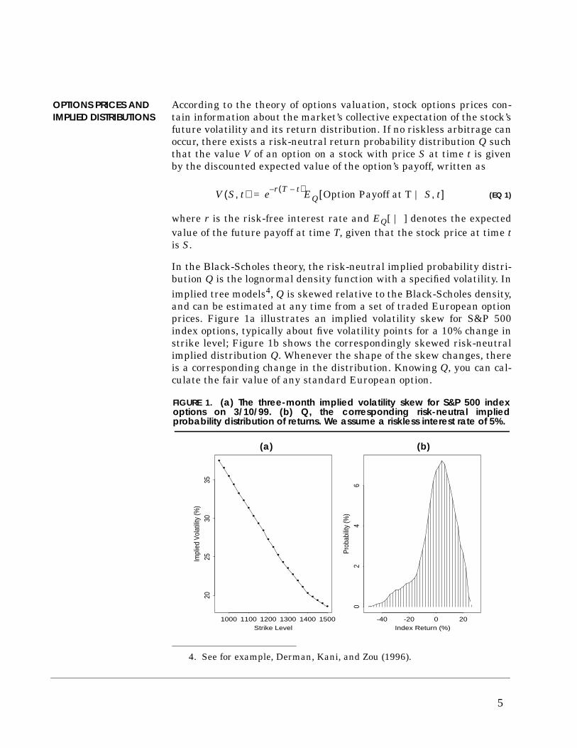
In the Black-Scholes theory, the risk-neutral implied probability distri-bution Q is the lognormal density function with a specified volatility. Inimplied tree models4, Q is skewed relative to the Black-Scholes density,and can be estimated at any time from a set of traded European optionprices. Figure 1a illustrates an implied volatility skew for S&P 500index options, typically about five volatility points for a 10% change instrike level; Figure 1b shows the correspondingly skewed risk-neutralimplied distribution Q. Whenever the shape of the skew changes, thereis a corresponding change in the distribution. Knowing Q, you can cal-culate the fair value of any standard European option.

4. See for example, Derman, Kani, and Zou (1996).

V S t,( ) e r T t–( )– EQ Option Payoff at T | S t,[ ]=

FIGURE 1. (a) The three-month implied volatility skew for S&P 500 indexoptions on 3/10/99. (b) Q, the corresponding risk-neutral impliedprobability distribution of returns. We assume a riskless interest rate of 5%.

••••

••

••

••

••

••

••

••

•

••

••

Strike Level

Impl

ied

Vola

tility

(%)

1000 1100 1200 1300 1400 1500

2025

3035

Index Return (%)

Prob

abilit

y (%

)

-40 -20 0 20

02

46

(a) (b)

5

STOCK RETURNS ANDHISTORICALDISTRIBUTIONS

Stock options’ prices determine the implied distribution of stockreturns. Independently, we can also observe the actual distribution ofstock. Consider the historical series Si of daily closing prices of a stockor stock index. We can construct the rolling series of continuously com-pounded stock returns Ri from day i for a subsequent period of N trad-ing days by calculating

(EQ 2)

Figure 2 shows the distribution of actual three-month S&P 500 returnsfor periods both before and since the 1987 stock market crash, wherethe latter period includes the crash itself.

The pre-crash return distribution is approximately symmetric and nor-mally distributed. In contrast, the post-crash distribution (1987-crashdata included) has a higher mean return and a lower standard devia-tion, as well as an asymmetric secondary peak at its lower end.

There is a rough similarity in shape between the implied distributionof Figure 1b, whose mean reflects the risk-free rate at which its optionswere priced, and the historical distribution of Figure 2b, whose (differ-ent) mean is the average historical return over the post-crash period.

Ri

Si N+

Si---------------log=

Index Return (%)

Pro

babi

lity

(%)

-20 0 20

01

23

4

Index Return (%)

Pro

babi

lity

(%)

-20 0 20

01

23

45

6

mean =1.8%std. div. = 7.3%

mean = 3.3%std. div. = 7.8%

FIGURE 2. Three-month, S&P 500 index, observed return distributions.(a) Pre-1987 crash (Jan. 1970 to Jan. 1987); (b) Post-1987 crash (June 1987to June 1999)

(a) (b)

6

Options theory does not enforce an unambiguous link between histori-cal and implied distributions. Nevertheless, historical distributions,suitably interpreted, can provide plausible information about fairoptions prices. Our aim in this paper is to develop a heuristic but logi-cal link between the two distributions, utilizing the notions of marketequilibrium and uncertainty.

7

MAXIMALUNCERTAINTY ANDMARKET EQUILIBRIUM

Markets are supposed to settle into equilibrium when supply equalsdemand, when there are equal numbers of buyers and sellers at someprice. In an efficient market, the potential buyers of a stock must thinkthe stock is cheap, and potential sellers must think it rich. This differ-ence of opinion means that, in equilibrium, the distribution of expectedreturns displays great uncertainty.

How do we quantify this simple intuition that equilibrium involvesuncertainty in the expected return distribution?

Entropy as a Measureof Uncertainty

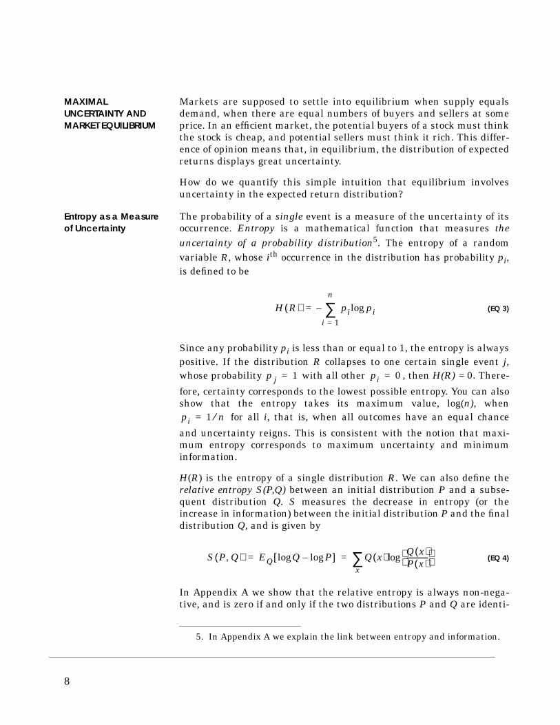
The probability of a single event is a measure of the uncertainty of itsoccurrence. Entropy is a mathematical function that measures theuncertainty of a probability distribution5. The entropy of a randomvariable R, whose ith occurrence in the distribution has probability pi,is defined to be

(EQ 3)

Since any probability pi is less than or equal to 1, the entropy is alwayspositive. If the distribution R collapses to one certain single event j,whose probability with all other , then H(R) = 0. There-

fore, certainty corresponds to the lowest possible entropy. You can alsoshow that the entropy takes its maximum value, log(n), when

for all i, that is, when all outcomes have an equal chance

and uncertainty reigns. This is consistent with the notion that maxi-mum entropy corresponds to maximum uncertainty and minimuminformation.

H(R) is the entropy of a single distribution R. We can also define therelative entropy S(P,Q) between an initial distribution P and a subse-quent distribution Q. S measures the decrease in entropy (or theincrease in information) between the initial distribution P and the finaldistribution Q, and is given by

(EQ 4)

In Appendix A we show that the relative entropy is always non-nega-tive, and is zero if and only if the two distributions P and Q are identi-

5. In Appendix A we explain the link between entropy and information.

H R( ) pi pilogi 1=

n

∑–=

p j 1= pi 0=

pi 1 n⁄=

S P Q,( ) EQ Q Plog–log[ ] Q x( ) Q x( )P x( )-------------

logx∑= =

8

cal. This agrees with our intuition that any change in a probabilitydistribution conveys some new information. The relative entropybetween two distributions measures the information gain (or reductionin uncertainty) after a distribution change. Thus, minimum relativeentropy corresponds to the least increase in information.

The Risk-NeutralizedHistorical Distribution

Consider a stock option with time to expiration T on a stock whose spotprice is . To value the option, we need to average the option payoff

over the risk-neutral probability density . In theory, Q( )

is found by solving the differential equation that constrains the instan-taneously hedged option to earn the instantaneously riskless return. Inthe Black-Scholes world, a stock’s future probability distribution isassumed to be lognormal, and consequently, though not obviously, Q( )itself is a lognormally distributed probability density, and its optionsprices have no volatility skew.

This theoretical lack of skew conflicts with the data from markets,where stocks and indexes that have sufficiently liquid out-of-the-money strikes display clear, and often large, skews. How can we esti-mate a suitable risk-neutral probability density that is more consistentwith market skews than the Black-Scholes lognormal distribution?

It is natural to turn for insight to the distribution of actual returns,. The two distributions Q( ) and P( ) cannot be strictly

identical, because the expected value of the stock price under the risk-neutral distribution Q( ) at any time must be the stock’s current for-ward price, as determined by the current risk-free rate, whereas theexpected value of the stock price under P( ) is the average historical for-ward price, which bears no relation to current risk-free rates.

The rigorous way to obtain Q( ) from the past evolution of stock pricesis to obtain fair historical options prices for a variety of strikes by sim-ulating the instantaneously riskless hedging strategy over the life ofthese options, and to then infer the risk-neutral density that matchesthese prices. This requires a detailed knowledge of every past instantof the stock price evolution, at all times and market levels, and is time-consuming, difficult, error-prone and ultimately impractical.

Instead, we will estimate the current risk-neutral return distributionQ( ) for a stock from its historical distribution P( ) by assuming that thelatter is a plausible estimate for the former, and then requiring thatthe relative entropy S(P,Q) between the distributions is minimized. Weimpose this criterion in order to avoid any spurious increase in appar-ent information in creating the risk-neutral distribution from the his-torical distribution. We perform the minimization subject to the risk-

S0

Q S0 0 ST T,;,( )

P S0 0 ST T,;,( )

9

neutrality constraint, that is, the condition that the expected value ofthe stock price under the risk-neutral distribution Q( ) is consistentwith the stock’s current forward price6. We call Q( ) found in this waythe risk-neutralized historical distribution7, or the RNHD. It isour plausible guess for the distribution to use in options valuation,given our knowledge of the past. Our knowledge of a stock’s historicalvolatility, the second moment of its distribution, is often used to esti-mate options values using the Black-Scholes formula. Here we go onestep further by using the entire historical return distribution. Adescription of the general approach outlined here can also be found inStutzer (1996).

It is possible to impose further constraints on Q( ). If you believe thatthe current at-the-money volatility for some particular stock is fair, youcan constrain the distribution Q( ) to match not only the stock forwardprice, but also to match the current at-the-money implied volatility. Wedenote this additionally constrained distribution by Qatm( ), and referto it as the at-the-money-consistent, risk-neutralized historicaldistribution, or RNHDATM. It can be used to compare the relativevalues of options with different strikes on one underlyer, assumingthat at-the-money volatility is fair.

Appendix B states the minimization condition on Q( ) in mathematicalterms. In Appendix C we present a model of an Arrow-Debreu economyand show that it is possible to obtain the risk-neutralized historicaldistribution by optimally allocating investors’ wealth under an equilib-rium condition with an exponential utility function.

Having obtained our estimate of the risk-neutral distribution, we canestimate the fair price for any standard option as the discountedexpected value of its payoff at expiration. We then extract the fairimplied volatility as the volatility which equates the Black-Scholesoption price to the estimated fair price. This procedure can be repeatedfor all strikes and maturities to yield an entire fair implied volatilitysurface.

6. Several authors have studied the relevance of entropy in financial eco-nomics and derivatives pricing. See Stutzer (1996), Derman et al.(1997), Buchen and Kelly (1996), and Gulko (1996).

7. For a normal historical distribution of simply compounded returns, onecan show that the risk-neutralized historical distribution obtained byentropy minimization is equivalent to a translation of the historical dis-tribution to re-center it at the appropriate risk-neutral rate, withoutaltering its shape. This translation invariance of the shape in movingfrom the historical to the risk-neutral distribution does not hold in gen-eral.

10

APPLICATIONS OFTHE RISK-NEUTRALIZEDHISTORICALDISTRIBUTION

The RNHD contains information which can be used to estimate thevalue of illiquid options whose prices are unobtainable, as well as tocompare the relative value of options with known market prices. Wepresent several representative examples below.

Is The Index ImpliedVolatility Skew Fair?

Since the 1987 crash, equity index markets have displayed a pro-nounced, persistent implied volatility skew. Is this skew fair? Are theoptions prices determined by the skew justified by historical returns?Figure 3a shows the risk-neutralized three-month S&P 500 return dis-tribution for the pre-crash period corresponding to Figure 2a, con-structed using our method of relative entropy minimization. Figure 3bshows the same distribution corresponding to the post-crash era of Fig-ure 2b. The post-crash distribution has a substantially longer tail atlow returns than the pre-crash distribution.

Skew slopes seem more stable than volatility levels. Therefore, we willfocus here on the relation between the implied volatilities of differentstrikes that follows from these distributions, and pay little attention tothe prevailing absolute level of implied volatility. We estimate the fairvolatility skew by using the distributions of Figure 3 to calculateoptions prices, and by then converting these options prices to Black-Scholes implied volatilities.

The results are shown in Figure 4. The pre-crash skew is approxi-mately flat, but the post-crash volatilities increase for low strikes, witha slope similar to actual index skews in stable markets. The observeddegree of skew, about five to six volatility points per 10% change in

Index Return (%)

Pro

babi

lity

(%)

-20 0 20

01

23

4

Index Return (%)

Pro

babi

lity

(%)

-40 -20 0 20

02

46

FIGURE 3. The three-month risk-neutral distribution of S&P 500 returnsconstructed from the empirical distributions of Figure 2 using a 6% risklessrate. (a) Pre-crash (b) Post-crash.

(a) (b)

11

strike level, seems approximately fair in the light of post-crash marketbehavior. Our fair post-crash skew is bilinear and more convex thanthe recent skew of Figure 1a, but index markets do sometimes displayskews like that of Figure 4.

We find that estimated one-month skews tend to resemble a smilemore than a skew: our fair implied volatilities of both out-of-the-moneycalls and puts for one-month expirations exceed at-the-money volatili-ties. Short-dated index options often display this type of behavior. Wehave applied our method to several other major stock indexes andfound that their fair volatility skews are roughly consistent withobserved market skews during normal market periods, as shown inTable 1.

FIGURE 4. The fair implied volatility skew for three-month S&P 500 options ascalculated from the risk-neutralized historical distributions of Figure 3.

Strike Level

Vol

atili

ty (%

)

90 95 100 105 110

1012

1416

1820

2224

post-crashpre-crash

TABLE 1. Comparison of actual skews with estimated fair volatility skews forthree major indexes. The spread shown is the difference in volatility pointsbetween a 25-delta put and a 25-delta call.

Index NormalaSpread

a. Average during normal market conditions (excluding the periods ofextreme volatility in late October 1997 and August-September 1998).

Extremeb

Spread

b. Average during periods of extreme market volatility.

Fairc

Spread

c. Based on historical returns over the period June 1987 to June 1999.

SPX 4-7% 14% 6.0%

DAX 3-6% 10% 3.5%

FTSE 2-6%. 10% 4.0%

12

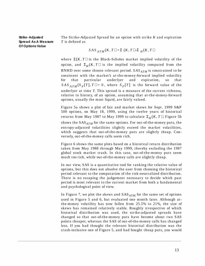
Strike-AdjustedSpread As A MeasureOf Options Value

The Strike-Adjusted Spread for an option with strike K and expirationT is defined as

where is the Black-Scholes market implied volatility of theoption, and is the implied volatility computed from the

RNHD over some chosen relevant period. SASATM is constrained to beconsistent with the market’s at-the-money-forward implied volatilityfor that particular underlyer and expiration, so that

, where is the forward value of the

underlyer at time T. This spread is a measure of the current richness,relative to history, of an option, assuming that at-the-money-forwardoptions, usually the most liquid, are fairly valued.

Figure 5a shows a plot of fair and market skews for Sept. 1999 S&P500 options, on May 18, 1999, using the twelve years of historicalreturns from May 1987 to May 1999 to calculate . Figure 5b

shows the SASATM for the same options. For out-of-the-money puts, theentropy-adjusted volatilities slightly exceed the market volatilities,which suggests that out-of-the-money puts are slightly cheap. Con-versely, out-of-the-money calls seem rich.

Figure 6 shows the same plots based on a historical return distributiontaken from May 1988 through May 1999, thereby excluding the 1987global stock market crash. In this case, out-of-the-money puts seemmuch too rich, while out-of-the-money calls are slightly cheap.

In our view, SAS is a quantitative tool for ranking the relative value ofoptions, but this does not absolve the user from choosing the historicalperiod relevant to the computation of the risk-neutralized distribution.There is no escaping the judgement necessary to decide which pastperiod is most relevant to the current market from both a fundamentaland psychological point of view.

In Figure 7, we plot the skews and SASATM for the same set of optionsused in Figure 5 and 6, but evaluated one month later. Although at-the-money volatility has now fallen from 25.5% to 21%, the size ofskews has remained relatively stable. Roughly irrespective of whichhistorical distribution was used, the strike-adjusted spreads havechanged so that out-of-the-money puts have become about two SASpoints cheaper, whereas the SAS of out-of-the-money calls has changedless. If you had thought the relevant historical distribution was thecrash-inclusive one of Figure 5, and had bought cheap puts, you would

SASATM K T,( ) Σ K T,( ) ΣH K T,( )–=

Σ K T,( )ΣH K T,( )

SASATM SF T[ ] T,( ) 0= SF T[ ]

ΣH K T,( )

13

Strike Level

Vol

atili

ty (

%)

1200 1250 1300 1350 1400 1450

2224

2628

3032

"fair skew" market skew

Strike LevelS

AS

(%

)1200 1250 1300 1350 1400 1450

-0.5

0.0

0.5

1.0

FIGURE 5. (a) Fair and market skews for S&P 500 index options on May 18,1999. (b) SASATM for the same options.The options considered expire on September 17, 1999. Both fair andmarket implied volatilities are constrained to match at the money,forward. The RNHD is constructed using returns from May 1987 to May1999, including the 1987 crash.

(a) (b)

Strike Level

Vol

atili

ty (

%)

1200 1250 1300 1350 1400 1450

2426

2830

"fair skew" market skew

Strike Level

SA

S (

%)

1200 1250 1300 1350 1400 1450

02

46

FIGURE 6. (a) Fair and market skews for S&P 500 index options on May 18,1999. (b) SASATM for the same options.The options considered expire on September 17, 1999. Both fair and marketimplied volatilities are constrained to match at the money, forward. TheRNHD is constructed using returns from May 1988 to May 1999, therebyexcluding the 1987 crash.

(a) (b)

14

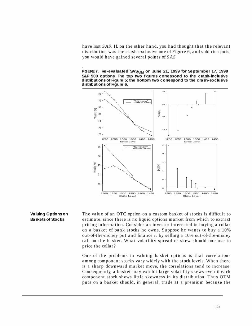
have lost SAS. If, on the other hand, you had thought that the relevantdistribution was the crash-exclusive one of Figure 6, and sold rich puts,you would have gained several points of SAS

.

Valuing Options onBaskets of Stocks

The value of an OTC option on a custom basket of stocks is difficult toestimate, since there is no liquid options market from which to extractpricing information. Consider an investor interested in buying a collaron a basket of bank stocks he owns. Suppose he wants to buy a 10%out-of-the-money put and finance it by selling a 10% out-of-the-moneycall on the basket. What volatility spread or skew should one use toprice the collar?

One of the problems in valuing basket options is that correlationsamong component stocks vary widely with the stock levels. When thereis a sharp downward market move, the correlations tend to increase.Consequently, a basket may exhibit large volatility skews even if eachcomponent stock shows little skewness in its distribution. Thus OTMputs on a basket should, in general, trade at a premium because the

Strike Level

Volat

ility (%

)

1200 1250 1300 1350 1400 1450

1820

2224

2628

30"fair skew" market skew

Strike Level

SAS (

%)

1200 1250 1300 1350 1400 1450

-2-1

01

Strike Level

Volat

ility (%

)

1200 1250 1300 1350 1400 1450

2022

2426

28 "fair skew" market skew

Strike Level

SAS (

%)

1200 1250 1300 1350 1400 1450

01

23

45

FIGURE 7. Re-evaluated SASATM on June 21, 1999 for September 17, 1999S&P 500 options. The top two figures correspond to the crash-inclusivedistributions of Figure 5; the bottom two correspond to the crash-exclusivedistributions of Figure 6.

15

increasing correlations in a down market makes the basket return dis-tribution skewed to the lower end. How do we model this effect? We uti-lize the information embedded in the historical time series of thebasket.

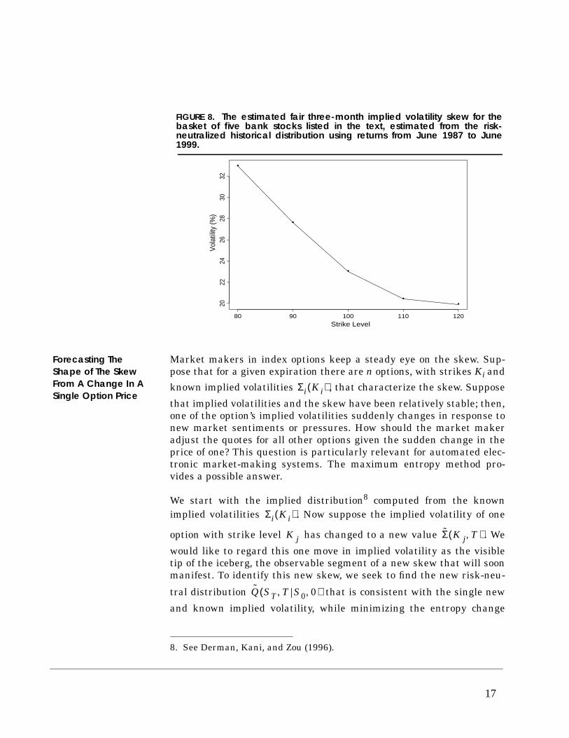
To be specific, we consider an example in which the basket consists ofan equal number of shares of five bank stocks: J.P. Morgan, WellsFargo, Bank One, Bank America, and Chase. We first retrieve the his-torical data for all five stocks and aggregate them to form the timeseries of basket returns and their historical distribution. We use histor-ical data from June 1987 to June 1999 in this example. By minimizingthe relative entropy, we convert the historical distribution into an esti-mate of the risk neutral distribution. Figure 8 displays the estimatedthree-month implied volatility skew for the bank basket calculatedfrom the risk-neutral distribution. The volatility spread between the10% OTM call and the 10% OTM put is approximately seven volatilitypoints. In the absence of any market information on the price of optionson this basket with a variety of strikes, this seems a useful method ofobtaining some sense of the appropriate skew. We note that in usingthis approach, we managed to bypass the problem of predicting futurecorrelations between the component stocks in the basket, a major hur-dle in valuing basket options. In this particular example, the three-month correlations between the stocks in the basket almost doubledduring the Fall of 1998 following the Russian currency devaluation.Our approach takes into account the changes in correlations embeddedin the basket time series.

We have also applied our model to options on the BKX index (a basketof 24 large U.S. banks with options listed on the Philadelphiaexchange). We constructed a basket with the same weighting as theBKX index and calculated both its empirical return distribution and itsestimated risk-neutral distribution. The resulting three-month volatil-ity skew is close to the skew observed in the listed options market,even when the at-the-money volatility levels differ. This further dem-onstrates the reasonableness of our approach.

16

Forecasting TheShape of The SkewFrom A Change In ASingle Option Price

Market makers in index options keep a steady eye on the skew. Sup-pose that for a given expiration there are n options, with strikes Ki and

known implied volatilities , that characterize the skew. Suppose

that implied volatilities and the skew have been relatively stable; then,one of the option’s implied volatilities suddenly changes in response tonew market sentiments or pressures. How should the market makeradjust the quotes for all other options given the sudden change in theprice of one? This question is particularly relevant for automated elec-tronic market-making systems. The maximum entropy method pro-vides a possible answer.

We start with the implied distribution8 computed from the knownimplied volatilities . Now suppose the implied volatility of one

option with strike level has changed to a new value . We

would like to regard this one move in implied volatility as the visibletip of the iceberg, the observable segment of a new skew that will soonmanifest. To identify this new skew, we seek to find the new risk-neu-

tral distribution that is consistent with the single new

and known implied volatility, while minimizing the entropy change

FIGURE 8. The estimated fair three-month implied volatility skew for thebasket of five bank stocks listed in the text, estimated from the risk-neutralized historical distribution using returns from June 1987 to June1999.

•

•

•

••

Strike Level

Vol

atili

ty (%

)

80 90 100 110 120

2022

2426

2830

32

8. See Derman, Kani, and Zou (1996).

Σi Ki( )

Σi Ki( )

K j Σ̃ K j T,( )

Q̃ ST T S0 0,,( )

17

between the old and new distributions. Once the new risk-neutral dis-tribution is obtained, we can update the quotes for the rest of theoptions by valuing them off the new distribution.

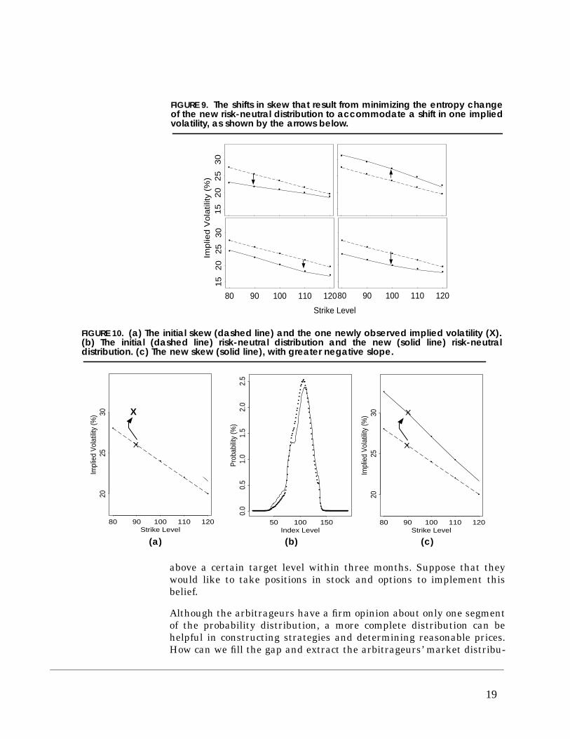
Here are some examples. Consider a hypothetical index whose currentvalue is 100. Suppose the three-month, at-the-money volatility is 24%,and the three-month skew is linear in strike with a slope correspond-ing to a two-volatility-point increase per ten-strike-point decline, asdisplayed in Figure 10a. The heavy X in the figure shows the one newlyobserved implied volatility, assumed to rise of four implied volatilitypoints, from 26% to 30%, for the 90-strike put. Figure 10b shows thechange in the risk-neutral implied distribution obtained by minimizingthe change in distributional entropy consistent with one new impliedvolatility. The increase in 90-strike implied volatility has led to a sig-nificant hump in the risk-neutral distribution below the 90 level.Finally, Figure 10c shows both the old and new skews, the latter com-puted from the new risk-neutral distribution. The new estimated skewdiffers from the old in a non-obvious way: it has not shifted parallel toaccommodate the one new item of information, but instead suggeststhat the skew slope will increase as a response to this shock.

Figure 9 shows several more examples where the volatility at one par-ticular strike is shocked. Note that shifts in at-the-money volatilityseem to lead to parallel shifts in the skew, whereas shifts in out-of-the-money volatility lead to changes in slope as well as level.

End-of-Day Mark ToMarket

At the end of a trading day, volatility traders need to re-mark all oftheir options positions. Often, only the liquid strikes have traded closeto the end of the day, and, if the last traded option has undergone a sig-nificant change in implied volatility, one needs to estimate the appro-priate skew for the remaining, less liquid options, based on the newinformation. Our model of minimizing the relative entropy provides aready solution to the problem. In the examples shown in Figure 9, onecould plausibly mark to market the rest of options using the solid linesas our best guesses for closing volatilities.

Filling Gaps InInvestors’ MarketViews

Risk arbitrageurs, speculators, and other situation-driven investorsoften have very specific, but not necessarily complete, views on themarket. For instance, risk arbitrageurs taking a position in the stocksof two companies involved in a merger or acquisition may estimate a90% probability that the deal will be completed and the stock will move

18

above a certain target level within three months. Suppose that theywould like to take positions in stock and options to implement thisbelief.

Although the arbitrageurs have a firm opinion about only one segmentof the probability distribution, a more complete distribution can behelpful in constructing strategies and determining reasonable prices.How can we fill the gap and extract the arbitrageurs’ market distribu-

••

••

•

Imp

lied

Vo

latil

ity (

%)

15

20

25

30

••••

•

••

••

•

Strike Level

80 90 100 110 120

15

20

25

30

••

••

•

••

••

•

••

••

•

••

••

•

80 90 100 110 120

•••

••

FIGURE 9. The shifts in skew that result from minimizing the entropy changeof the new risk-neutral distribution to accommodate a shift in one impliedvolatility, as shown by the arrows below.

FIGURE 10. (a) The initial skew (dashed line) and the one newly observed implied volatility (X).(b) The initial (dashed line) risk-neutral distribution and the new (solid line) risk-neutraldistribution. (c) The new skew (solid line), with greater negative slope.

•

•

•

•

•

Strike Level

Impl

ied

Vola

tility

(%)

80 90 100 110 120

2025

30

•

•

•

•

X

X

(b)

•••••••••••••••••••••••••••••••••••••••••••••••••••

••••

••••••••••••••••

••••••••••••

••••••••••••••••

••••••••

•

•••••••••••••••••••••••••••••••••••••••••••••••••••••••••••••••

Index Level

Prob

abilit

y (%

)

50 100 150

0.0

0.5

1.0

1.5

2.0

2.5

•

•

•

•

•

Strike Level

Impl

ied

Vola

tility

(%)

80 90 100 110 120

2025

30

•

•

•

•

X

X

(a) (b)

X

(a) (b) (c)

19

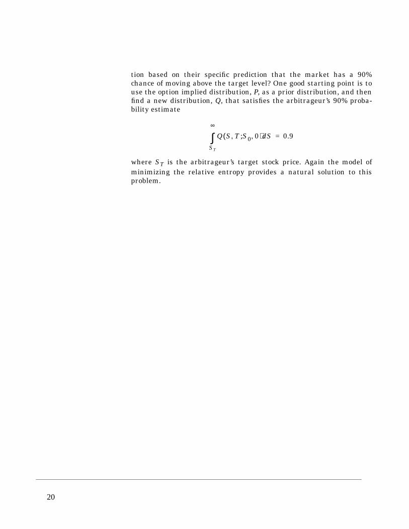
tion based on their specific prediction that the market has a 90%chance of moving above the target level? One good starting point is touse the option implied distribution, P, as a prior distribution, and thenfind a new distribution, Q, that satisfies the arbitrageur’s 90% proba-bility estimate

where ST is the arbitrageur’s target stock price. Again the model ofminimizing the relative entropy provides a natural solution to thisproblem.

Q S T S0 0,;,( ) Sd

ST

∞

∫ 0.9=

20

CONCLUDINGREMARKS

Investors in equity options have two problems that compound eachother: the many thousands of equity underlyers and the presence of aunique volatility skew for each of them. For many thinly-traded singlestock and basket options, it is difficult or impossible to get adequateinformation on the market skew.

In this paper, we have employed a systematic, semi-empirical methodfor estimating the risk-neutral distribution of any underlyer, stock orbasket, whose historical returns are available. This method, originallyused by Stutzer (1996), involves the determination of a new, risk-neu-tralized historical distribution (RNHD) for an underlyer by minimizingthe relative entropy between the historical distribution and the risk-neutral distribution.

Using the RNHD, we can compute the estimated fair implied volatili-ties of options of any strike and expiration. We can apply this methodto illiquid or thinly-traded derivatives where market prices areunavailable.

We have defined a new metric, the strike-adjusted spread, or SAS, forgauging the value of options whose prices are known. SAS is the differ-ence between an option’s implied volatility and its fair volatility asestimated using the RNHD. This spread represents the richness in vol-atility points of an option, compared to the history of its underlyer.Most often, in liquid markets, we calibrate the SAS to be consistentwith current at-the-money volatility, so that it becomes a measure ofskew richness as compared with history. The SAS ranking cannot beused blindly; it depends on the user’s selection of the historical periodmost relevant to the current market.

There are many other applications of the method of minimal relativeentropy we have illustrated in this paper. One may choose as a prior anexisting options’ implied distribution, or any other distribution reflect-ing subjective market views. We hope that this practical method andits extensions will help investors make more rational decisions aboutvalue in volatility markets.

21

APPENDIX A:INFORMATION ANDENTROPY

Probability measures the uncertainty about the occurrence of a singlerandom event. For a given random variable X, what can we deducefrom a single observation that ?

Information Information9 changes our view of the world. It seems obvious that theamount of information conveyed by the observation that shoulddepend on how likely this event was previously assumed to be. If astock was expected to go up the next day by everyone, and it actuallywent down, the surprising outcome is certainly more informative thanthe expected outcome. We want to quantify the notion of events provid-ing information.

We seek a function that can represent the information providedby the occurrence of the event whose probability was assumedto be p. We require that be a non-negative and decreasing func-tion of p; our intuition says that I( ) is non-negative because the occur-rence of the event must provide some information; similarly, I( ) mustdecrease with increasing p because the more likely we thought theevent was, the less information its occurrence provides.

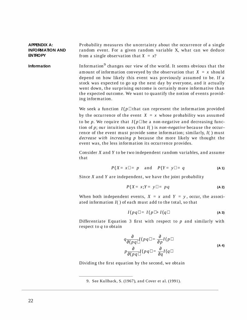
Consider X and Y to be two independent random variables, and assumethat

(A 1)

Since X and Y are independent, we have the joint probability

(A 2)

When both independent events, and , occur, the associ-ated information I( ) of each must add to the total, so that

(A 3)

Differentiate Equation 3 first with respect to p and similarly withrespect to q to obtain

(A 4)

Dividing the first equation by the second, we obtain

X x=

9. See Kullback, S. (1967), and Cover et al. (1991).

X x=

I p( )X x=

I p( )

P X x=( ) p and P Y y=( ) q= =

P X x Y y=;=( ) pq=

X x= Y y=

I pq( ) I p( ) I q( )+=

qpq( )∂∂ I pq( )

p∂∂ I p( )=

ppq( )∂∂ I pq( )

q∂∂ I q( )=

22

or

(A 5)

Since q and p are independent variables, each term in Equation 5 mustbe a constant, denoted , so that

Since an event with probability q = 1 provides no information, .Since , and since we required that I( ) be a non-negative anddecreasing function of q, the constant c must be positive. From now onwe set , which defines the conventional size of a unit of informa-tion. The information provided by the occurrence of an event whoseprobability was p is therefore given by

(A 6)

Entropy The probability assigned to a single event is a measure of the uncer-tainty of its occurrence. The entropy of a random variable R, whose ith

occurrence in the distribution has probability pi, is defined to be theexpected value of the information from the occurrence of an event inthe distribution, namely

(A 7)

Since any probability pi is less than or equal to 1, the entropy is alwayspositive.

A large expected value of information means that the distribution wasbroad, with a wide spread of probabilities. A small expected informa-tion means the distribution was relatively narrow, so that not muchinformation can be gained from the occurrence of an expected event.Qualitatively, therefore, you can see that H represents the uncertaintyin the distribution: large (small) average information H corresponds to

qp---- p∂

∂ I p( )

q∂∂ I q( )

-------------------=

qq∂

∂ I q( ) pp∂

∂ I p( )=

c–

I q( ) c q( )ln– A+=

A 0=

0 q 1≤ ≤

c 1=

I p( ) p( )ln–=

H R( ) pi pilogi 1=

n

∑–=

23

high (low) uncertainty. Entropy is the mathematical function that mea-sures the uncertainty of a distribution. This is consistent with our intu-ition that maximum entropy corresponds to maximum uncertainty.

If the distribution collapses to one certain single event j whose, all other , then H = 0, a minimum. You can also show

that the entropy takes its maximum value, log(n), when for

all i, i.e. when all outcomes have an equal chance and there is maximaluncertainty.

Having established the notion that the entropy of a probability distri-bution reflects the expected amount of information, we can now quan-tify the information gained upon changing the distribution as a resultof new information. Let us assume we have a prior distribution of arandom variable X which we denote by P. Upon arrival of new informa-tion, a posterior distribution Q is established. What is the consequentreduction in uncertainty (decrease in entropy) in this process? Oneobvious choice is the relative entropy:

(A 8)

The -log( ) function is convex, so that, by Jensen’s inequality, the aver-age of the is greater than the -log( ) of the average of

. Therefore,

Therefore, is strictly non-negative, and is zero if and only ifidentically. can be thought of as a “distance” between

two probability distributions.

To maintain maximum uncertainty given some new information, ourgoal is to minimize this relative entropy or “distance” between the priorand posterior distributions.

p j 1= pi 0=

pi 1 n⁄=

S P Q,( ) EQ Q Plog–log[ ] qiqipi-----log

i∑= qi

piqi-----log

i∑–= =

pi qi⁄( )log–

pi qi⁄( )

S P Q,( ) qi

piqi-----

i∑log–> pi( )

i∑log– 1log– 0= = =

S P Q,( )P Q≡ S P Q,( )

24

APPENDIX B:DETERMINING THERISK-NEUTRALDISTRIBUTION FROMHISTORICAL RETURNS

Consider a stock whose spot price is . Assume that investors believe

the future return distribution of the asset is given by a prior. Our goal is to infer the risk-neutral distribution

from subject to the constraint that the

mean of the risk-neutral stock distribution must equal the stock for-ward price. We determine the risk-neutral distribution by minimizingthe relative entropy between P( ) and Q( ) subject to Q( ) satisfying theforward condition.

We seek so that

(B 1)

such that

(B 2)

and

(B 3)

where is the current riskless interest rate.

In some cases we will also have a good idea of the current value of thestock’s at-the-money implied volatility. In that case we will add toEquation B2 and Equation B3 the further constraint that the at-the-money implied volatility produced by the distribution Q( ) is equal tothe at-the-money implied volatility of the stock.

Solving the above equations, we obtain the risk-neutral distribution

(B 4)

where the constant can be found numerically by ensuring that it sat-isfies the forward condition

(B 5)

Because in Equation B4 is always non-negative, so is .

S0

P S0 0 ST T,;,( )

Q S0 0 ST T,;,( ) P S0 0 ST T,;,( )

Q S0 0 ST T,;,( )

Min S P Q,( ) EQQ S( )P S( )-------------

log=

Q ST( )ST STd∫ S0erf T=

Q ST( ) STd∫ 1=

rf

Q S0 0 ST T,;,( )P S0 0 S;, T T,( )

P S( ) λ– S( )exp Sd∫--------------------------------------------------- λ– ST( )exp=

λ

Qλ S0 0 ST T,;,( )ST STd∫ S0erf T=

P ST( ) Q ST( )

25

APPENDIX C:A DERIVATIVE ASSETALLOCATION MODELAND THE EQUILIBRIUMRISK-NEUTRAL DENSITY

In this appendix, we present a simple derivative asset allocation modeland give a possible financial economic interpretation of the resultsobtained in this paper based on the maximal entropy principle. Con-sider an economy in equilibrium with total investor wealth W0. Thereis a market for an equity index, a riskless bond, and a complete rangeof derivative instruments on the index. We assume that there is a rep-resentative investor10 with a subjective market view expressedthrough a conditional probability density , where is

the spot index level. We also assume the return on the riskless bondover the period T is rf. The representative investor allocates a portionof the total initial wealth to the riskless bonds and the remainingwealth to the risky assets. Let α be the portion allocated to risklessbonds, and be the portion allocated to risky assets. Since therisky assets can be replicated with a portfolio of Arrow-Debreu securi-ties, the investor can simply find an optimal portfolio of Arrow-Debreusecurities. An Arrow-Debreu security with parameter E has a pricegiven by

(C 1)

where is the discount factor and is the

risk-neutral probability density. The payoff of the Arrow-Debreu secu-rity at the expiration date is, by definition,

(C 2)

Let be the portion of the fraction allocated to riskyassets that is invested in Arrow-Debreu security with parameter E. Atthe end of period T, the total investor wealth will be

(C 3)

where

(C 4)

Note that

(C 5)

10. See Constantinides (1982).

P S0 0 ST T,;,( ) S0

1 α–

π St t E T,;,( ) DQ S t E T,;,( )=

D 1 1 rf+( )⁄= Q St t E T,;,( )

π ST T E T,;,( ) δ ST E–( )=

ω E( )dE 1 α–

WT ST( ) W0 1 αrf 1 α–( ) ω E( )rE ST( ) Ed∫+ +[ ]=

rE ST( )π ST T E T,;,( ) π St t E T,;,( )–

π St t E T,;,( )-----------------------------------------------------------------------------≡

δ ST E–( )DQ S t E T,;,( )-------------------------------------- 1–=

Er E( )Q St t E T,;,( )d∫ rf=

26

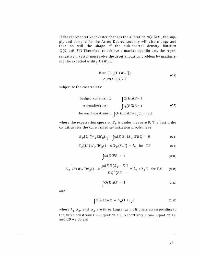
If the representative investor changes the allocation , the sup-ply and demand for the Arrow-Debreu security will also change andthus so will the shape of the risk-neutral density function

. Therefore, to achieve a market equilibrium, the repre-

sentative investor must solve the asset allocation problem by maximiz-ing the expected utility :

(C 6)

subject to the constraints:

(C 7)

where the expectation operator Ep is under measure P. The first orderconditions for the constrained optimization problem are

(C 8)

(C 9)

(C 10)

(C 11)

(C 12)

and

(C 13)

where are three Lagrange multipliers corresponding to

the three constraints in Equation C7, respectively. From Equation C8and C9 we obtain

ω E( )dE

Q St t E T,;,( )

U WT( )

Max Ep U WT( )[ ]{ }

α ω E( ) Q E( ),,{ }

budget constraint: ω E( ) E= 1d∫normalization: Q E( ) E= 1d∫

forward constraint: Q E( )E E=S0 1 rf+( )d∫

EP U' WT( )W0 rf ω E( )rE ST( ) Ed∫–( )[ ] 0=

EP U' WT( )W0 1 α–( )rE ST( )[ ] λ1 for E∀=

ω E( ) Ed∫ 1=

EP U' WT( )'W0 1 α–( )ω E( )δ ST E–( )

DQ2 E( )---------------------------------------- λ2 λ3E for E∀+=

Q E( ) Ed∫ 1=

Q E( )E Ed∫ S0 1 rf+( )=

λ1 λ2 and λ3, ,

27

(C 14)

and

(C 15)

From Equations C8, C14 and C15 we have

(C 16)

where

(C 17)

Using Equations C11, C15 and C16, we get

(C 18)

Using the constraints (C12) and(C13), Equation (C16) leads to

(C 19)

These results so far are independent of the particular functional formof the utility function as long as the utility function is monotonicallyincreasing and concave. We now specialize in an exponential utilitygiven by

(C 20)

Using Equations C16, C17, C18 and C20, one can show that

(C 21)

where constant c0 and c1 satisfy

(C 22)

EP U' WT( )rE ST( )[ ]λ1

W0 1 α–( )---------------------------=

EP U' WT( )[ ]λ1

W0 1 α–( )rf---------------------------------=

Q S0 t S;, T T,( )U' WT ST( )( )EP U' WT( )[ ]----------------------------------P S0 t ST T,;,( )=

WT E( ) W0 α 1 rf+( ) 1 α–( ) ω E( )DQ E( )-------------------+=

ω E( )Q E( )--------------

rf1 rf+---------------

λ2λ1------

λ3λ1------E+=

λ2λ1------

λ3λ1------S0 1 rf+( )+

1 rf+

rf---------------=

U WT( ) bWT–( ) with b 0>exp–=

Q St t E T,;,( ) P St t E T,;,( ) c0 c1E–( )exp=

c0 b– W0α 1 rf+( ) EP U' b⁄[ ]( )λ2

EP U' b⁄[ ]---------------------------–log–=

28

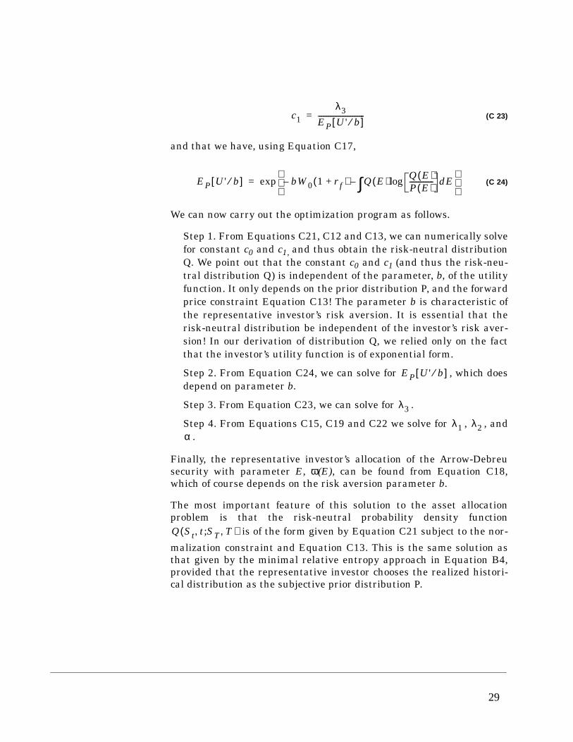
(C 23)

and that we have, using Equation C17,

(C 24)

We can now carry out the optimization program as follows.

Step 1. From Equations C21, C12 and C13, we can numerically solvefor constant c0 and c1, and thus obtain the risk-neutral distributionQ. We point out that the constant c0 and c1 (and thus the risk-neu-tral distribution Q) is independent of the parameter, b, of the utilityfunction. It only depends on the prior distribution P, and the forwardprice constraint Equation C13! The parameter b is characteristic ofthe representative investor’s risk aversion. It is essential that therisk-neutral distribution be independent of the investor’s risk aver-sion! In our derivation of distribution Q, we relied only on the factthat the investor’s utility function is of exponential form.

Step 2. From Equation C24, we can solve for , which doesdepend on parameter b.

Step 3. From Equation C23, we can solve for .

Step 4. From Equations C15, C19 and C22 we solve for , , and.

Finally, the representative investor’s allocation of the Arrow-Debreusecurity with parameter E, ω(E), can be found from Equation C18,which of course depends on the risk aversion parameter b.

The most important feature of this solution to the asset allocationproblem is that the risk-neutral probability density function

is of the form given by Equation C21 subject to the nor-

malization constraint and Equation C13. This is the same solution asthat given by the minimal relative entropy approach in Equation B4,provided that the representative investor chooses the realized histori-cal distribution as the subjective prior distribution P.

c1λ3

EP U' b⁄[ ]---------------------------=

EP U' b⁄[ ] bW0 1 rf+( )– Q E( ) Q E( )P E( )--------------log Ed∫–

exp=

EP U' b⁄[ ]

λ3

λ1 λ2α

Q St t ST T,;,( )

29

30

REFERENCES Buchen, P.W. and M. Kelly, 1996, Journal of Financial and Quantita-tive Analysis, 31, pp. 143 - 159.

Constantinides, G.M., 1982, The Journal Of Business, 55, No. 2.

Cover, T.M. and J.A. Thomas, 1991, Elements of Information Theory,New York, John Wiley & Sons.

Derman, E., I. Kani and J. Zou, 1996. The Local Volatility Surface,Financial Analysts Journal, July/August, pp. 25-36.

Derman, E., M. Kamal, I. Kani, and J. Zou, 1997, Is the Volatility SkewFair?, Goldman, Sachs Quantitative Strategies Research Notes

Gulko, L., 1996, Yale University Working Paper.

Kullback, S., 1967, Information Theory and Statistics, New York,Dover Publications, Inc.

Stutzer, M., 1996, A Simple Nonparametric Approach to DerivativeSecurity Valuation, J. of Finance, 51. pp. 1633 - 1652.

Stutzer, M., and M. Chowdhury, 1999, A Simple Non-ParametricApproach to Bond Futures Options Pricing, Journal of Fixed Income,March 1999, pp. 67-76.