a new method for leak detection in gas pipelines · pdf filea new method for leak detection in...

PB Oil and Gas Facilities • April 2015 April 2015 • Oil and Gas Facilities 97PB Oil and Gas Facilities • April 2015 April 2015 • Oil and Gas Facilities 1

A New Method for Leak Detection in Gas Pipelines

Kegang Ling, University of North Dakota; Guoqing Han and Xiao Ni, China University of Petroleum; Chunming Xu, China National Offshore Oil Corporation; and Jun He, Peng Pei, and Jun Ge, University of North Dakota

lower cost. It also has the advantages of monitoring the system con-tinuously and noninterference with pipeline operations. One of the limitations of the modeling method is that it requires flow param-eters, which are not always available. Leak detection from math-ematical modeling also has a higher uncertainty than that from physical inspection.

Many researchers have conducted investigations on gas transient flow in pipelines to detect leaks. Huber (1981) used a computer-based pipeline simulator for batch tracking, line balance, and leak detection in the Cochin pipeline system. The instruments installed in the pipeline and the simulator in the central control office made on-line, real-time surveillance of the line possible. The resulting model was capable of determining pressure, temperature, density, and flow profiles for the line. The simulator was based on mass balance, and thus required a complete set of variables to detect the leak.

Shell used physical methods to detect leaks in a 36-in.-diam-eter, 78-mile-long submarine pipeline near Bintulu, Sarawak (van der Marel and Sluyter 1984). The leaks were detected accurately by optical and acoustical equipment mounted on a remotely oper-ated vehicle, which was guided along the pipeline from a distance of 0.5 m above the pipeline. The disadvantages of this detection method are time consumption (15 days to finish detection), and the pipeline needed to be kept at a high pressure to obtain a relatively high signal/noise ratio. Sections of the pipeline were covered by a thick layer of selected backfill. This ruled out the use of the optical technology. It is also noted that the maximum water depth was 230 ft. Applications in a deepwater environment have not been tested.

Luongo (1986) studied the gas transient flow in a constant-cross-section pipe. He linearized the partial-differential equation and developed a numerical solution to the linear parabolic partial-differential equation. In his derivation, friction factor was calcu-lated from steady-state conditions (i.e., constant friction factor for transient flow). Luongo (1986) claimed that his linearization al-gorithm can save 25% in the computational time without a major sacrifice in accuracy when compared with other methods. The gov-erning equations used by Luongo (1986) required a complete data set of pressure and flow rate.

Massinon (1988) proposed a real-time transient hydraulic model for leak detection and batch tracking on a liquid-pipeline system on the basis of the conservation of mass, momentum, and energy, and an equation of state. Although this model can detect leaks in a timely manner, it required intensive acquisition of complete data sets, both in the space domain (the pipeline lengths between sen-sors are very short) and in the time domain (time interval between two consecutive measurements is short), which are impossible for many pipelines.

Mactaggart (1989) applied a compensated volume-balance method at a cost less than a transient-model-based leak detection for sour-gas-leak detection. The method is cost effective, but is ap-plied only to well-instrumented pipelines. Pressure and rate at the inlet and the outlet of the pipeline are required for this analysis.

Scott et al. (1999) modeled the deepwater leak in a multiphase production flowline. Their method can detect a multiphase leak, but

Copyright © 2015 Society of Petroleum Engineers

This paper (SPE 1891568) was accepted for presentation at the SPE/AAPG/SEG Unconventional Resources Technology Conference, Denver, 25–27 August 2014, and revised for publication. Original manuscript received for review 10 June 2014. Revised manuscript received for review 26 December 2014. Paper peer approved 28 January 2015.

Summary Two types of approaches—physical inspection and mathematical-model simulation—are used to identify a leak in a gas pipeline. The former method can result in an accurate detection of the location and the size of the leak, but comes with the expense of production shutdown and the high cost/long time to run the physical detection, which is very crucial in a long-distance gas pipeline. The latter ap-proach detects a gas leak by solving the governing equations, thus leading to quick evaluation at much lower costs, but with higher uncertainties. Our literature review indicates that a simple, prac-tical, and reliable method to detect a gas leak under the conditions of unknown inlet or outlet gas rate, or unknown inlet or outlet pres-sure, is highly desirable.

In this study, we develop single and multiple rate test methods to detect leaks in a gas pipeline. By conducting multiple rate tests, the location and size of leaks can be detected. The new method can be applied under the conditions of no inlet or outlet rate available or no inlet or outlet pressure available. Because these conditions are not uncommon in gas-pipeline transportation, our method provides a quick and low-computational-cost approach to detect leaks corre-sponding to different scenarios.

IntroductionBecause of its efficiency, cleanliness, and reliability, natural gas supplies nearly one-fourth of all energy used in the United States and is expected to increase by 50% within the next 20 years (An-derson and Driscoll 2000). New gas-delivery infrastructure is con-structed to transport more natural gas to terminals far away from the production site. At the same time, existing gas-delivery infrastruc-ture is aging rapidly. Ensuring natural-gas-infrastructure reliability is one of the critical needs for the energy sector. Therefore, the reli-able and timely detection of leakage from a newly-built gas pipeline during startup, and the failure of any part of the old pipeline, is crit-ical to the flow assurance of the natural-gas infrastructure.

Traditionally, there are two types of approaches to detecting leaks in a gas pipeline; one is physical inspection to identify the location and size of the leak, and the other is mathematical mod-eling with numerical simulation. Physical inspection consists of gas sampling; soil monitoring; flow-rate monitoring; and acoustic-, optical-, and satellite-based hyperspectral imaging. Usually, the physical inspection can result in an accurate detection of the lo-cation and size of a leak, but this comes with the expense of pro-duction shutdown and the high cost/long time to run the physical detection, which is very crucial in a long-distance gas pipeline. The mathematical-modeling approach detects a gas leak by solving the governing mass-conservation, momentum-conservation, and en-ergy-balance equations, thus leading to a quick evaluation at much

98 Oil and Gas Facilities • April 2015 April 2015 • Oil and Gas Facilities 992 Oil and Gas Facilities • April 2015 April 2015 • Oil and Gas Facilities 3

needs to identify the flow regime first. The flow regime can change along the pipeline. A multiphase leak also affects the flow regime and makes its prediction very difficult. Zhou and Adewumi (2000) in-cluded the kinetic-energy term in the governing equation and solved the partial-differential equation numerically. They formulated an ex-plicit five-point, second-order-accurate total-variation-diminishing scheme to capture the behavior of transient flow. Boundary and ini-tial conditions needed to be given in the simulation.

Sadovnychiy et al. (2005) discussed the development of a remote-detection system consisting of an infrared camera, a video camera, a laser spectrometer, and a global-positioning system for early detection of leaks in oil and gas pipelines. The remote system can detect small leaks. The disadvantages include reliance of the system on multiple sensitive and delicate instruments, which are susceptible to harsh environments or severe weather; and the need to develop an automation system for data acquisition, transmission, integration, and interpretation.

Reddy et al. (2006) built a dynamic simulation model by use of a transfer-function model for online state estimation and leak detection in a gas pipeline. The model reduced the computational time, while obtaining accurate state estimation from noisy mea-surements. The computation required all available measurements of pressure and flow rate.

Wang and Carroll (2007) analyzed the real-time data with a tran-sient model to detect gas- and liquid-pipeline leakage. Stochastic processing and noise filtering of the meter reading were used to re-duce the impact of noise. The correlations for diagnosing the leak location and amount are derived on the basis of the online real-time observation and the readings of pressure, temperature, and flow rate at both ends of the pipeline.

Gajbhiye and Kam (2008) used a mechanism model to de-tect leakage in a subsea pipeline under fixed pressure boundaries. The model compared the inlet and outlet flow-rate changes with fixed-pressure boundary conditions to detect leakage. Although the model can be applied to single- and multiphase flows, it needed pressures and flow rates at both ends of the line.

Elliott et al. (2008) showed the efficiency of leak detection by a spherical acoustic device called a SmartBall®, which has the ad-vantages of low cost, ease of deployment, and the ability to locate pinhole leaks immediately to within 1 m. This technique is limited by pipeline geometry. A long pipeline also requires long inspec-tion time to detect leakage. Launching and receiving SmartBalls are necessary, which may not be applicable in some conditions.

Hauge et al. (2009) used an adaptive Luenberger-type esti-mator to locate and quantify leakage given inlet velocity, pressure, and temperature and outlet velocity and pressure. The model was built in OLGA, a commercial software from Schlumberger (2014), which can handle multiphase flow and incorporated temperature dynamics. Pressure and rate at two ends of the pipeline are required for numerical calculation.

Bustnes et al. (2011) applied a commercial real-time transient model to detect leakage in a Troll field oil pipeline. The model can accept American Standard Code for Information Interchange (ASCII) input data and required no prior knowledge of the soft-ware-calculation method. However, the accuracy of leak detection for this method is low. Uncertainty because of transient pipeline operation is also an issue.

Eisler (2011) reviewed the leak-detection technologies applied to Artic subsea pipelines and recommend fiber-optic-cable tech-nology for pipelines under such conditions. This method can de-tect leaks promptly, but with a high cost for equipment, installation, and maintenance.

Vrålstad et al. (2011) compared five different leak-detection sys-tems that are suitable for continuous monitoring of a subsea tem-plate and elucidated the advantages and limitations of the different detection principles. Continuous monitoring by permanently in-stalled systems, flow-measurement devices, or inspection/sur-veying by sensors attached to mobile units were applied to detect

small leaks. The disadvantage is that a large number of sensors were installed in the line, thus increasing the cost significantly.

Balda Rivas and Civan (2013) used mass-balance and transient-flow models to detect leaks in liquid pipelines. The response times to the transient-flow operation were used to estimate leak location. Their model required intensive measurements of all variables.

In summary, existing methods are classified into two larger cat-egories: physical method and mathematical model. Physical detec-tion has the advantages of accuracy and high certainty. The online, real-time surveillance of pipelines and leak detection can be real-ized if monitoring equipment is installed in the pipeline. Because the physical method requires installation and maintenance of substantial levels of costly equipment on the pipeline, it may be excluded be-cause the high operating cost is not affordable and the long time taken to detect the leak is unacceptable because of the continuous loss of revenue, damage to facilities and environment, and possible loss of life. Sometimes, a harsh environment or severe weather can make the installation of detection instruments in the pipeline and/or physical inspections impossible. In some cases, remote locations that are dif-ficult to access make physical inspection unrealistic. The mathemat-ical model has the advantages of low cost and quick leak detection. Shutdown of the operation may not be required. The continuous on-line, real-time monitoring of the pipeline and leak identification are possible if the required data can be measured and transmitted to the central office simultaneously. The disadvantages of the mathemat-ical model are low accuracy and high uncertainty. High-quality and complete data sets are key factors of detecting leaks successfully. In practice, the mathematical model can be used to narrow down the possible leak interval before the physical inspection is conducted.

This literature review indicated that only a few studies provided a practical method for detecting gas leaks in pipelines without inlet or outlet flow rate or pressure. It is worthwhile to develop an ap-proach to locate a leak and evaluate its size under these conditions because, as oil and gas exploration and production move toward offshore, deep water, polar regions, and remote/frontier locations, it is not uncommon that metering equipment or pressure gauges would not be installed at the inlet and/or outlet of the pipeline in these fields. Even for onshore fields or fields with easy access, op-erators may choose not to install metering equipment to cut costs. In some gas-gathering systems, metering equipment is not installed in the branches that connect to the trunk lines. The flow rates are measured only in the trunk lines. In addition, the metering equip-ment and pressure gauges installed in the pipeline may be nonfunc-tioning. Although the percentage of these uncommon issues is low, the absolute number of pipelines without inlet or outlet pressure or flow rate can be large, considering the large number of oil and gas pipelines operated in the field. Furthermore, these issues might be-come common in the future when fields in harsh environments are developed. It is also noted that leakage in offshore and deepwater pipelines is difficult to locate and quantify. Therefore, we propose a new method to solve these issues.

Model DevelopmentIn this work, leak detection and localization are realized by cou-pling the gas-pipeline flow with the gas-leak flow. Multiple rate tests are conducted to solve the governing flow equations to eval-uate gas leak. Modeling of gas flow in pipelines and gas-leak flow are discussed in Appendices A and B, respectively.

Leak Detection for One Pipeline. Single and multiple rate tests are required to obtain flow parameters to solve the governing equa-tions to locate the gas leak and evaluate the gas-leak rate (or leak size) for different scenarios. The application of multiple-rate tests to different scenarios is discussed in the following subsections. Three assumptions are made in the analyses:

• Single gas phase flows in the pipeline.• Temperature profile along the pipeline is known.• Gas leak occurs in only one location.


The gas-leak rate is the difference between the inlet and the outlet gas rates. The location of the gas leak can be identified by di-mensionless analysis. To develop a general solution, we introduce three dimensionless variables: leak location, gas-leak rate, and pressure drop.

Dimensionless leak location is defined as the ratio of distance between leak locale and pipeline inlet to pipeline length, which is expressed as

LL

LDleakleak

, = , ..........................................................................(1)

where Lleak,D is the dimensionless leak location and Lleak is the leak location (measured from the inlet of the pipeline to the leak locale).

Dimensionless gas-leak rate is defined as the ratio of the gas-leak rate to the gas rate at the inlet of the pipeline, which is

qq

qDleakleak

inlet, = , ...........................................................................(2)

where qleak,D is the dimensionless gas-leak rate, qleak is the gas-leak rate, and qinlet is the gas rate at the inlet of the pipeline.

Dimensionless pressure drop is defined as the ratio of pressure drop through the pipeline under gas-leak conditions to pressure drop through the pipeline without leak, which is expressed as

∆ = ∆∆

pp

pDleak

no leak

, ........................................................................(3)

where ∆pD is the dimensionless pressure drop, ∆pleak is the pressure drop through the pipeline under gas-leak conditions, and ∆pno leak is the pressure drop through the pipeline without leak. Synthetic ex-amples are used to better illustrate the detection procedure. Table 1 lists the data used for the different scenarios described in the fol-lowing subsections.

Scenario 1: One Pipeline With Known Inlet and Outlet Rates and Known Inlet and Outlet Pressures. Only one flow-rate test is required to locate the gas leak. The analysis procedure is

1. Run Single Rate Test 1 and record the inlet and outlet gas rates and pressures.

2. Calculate the pressure drop in the pipeline, assuming that there is no leak in the pipeline, by use of Eq. A-1. It should be noted that the pressure drop without gas leak is the max-imum compared with gas-leak cases.

3. Assuming gas leakage at different locations with different leak sizes, calculate the pressure drops that correspond to the different leak locations and leak sizes. Also calculate the di-mensionless leak locations, dimensionless gas-leak rates, and the dimensionless pressure drops.

4. Plot the dimensionless pressure-drop/gas-leak-rate/leak-lo-cation type curves on the basis of the data gained in Steps 1, 2, and 3, as in Fig. 1.

5. Calculate the pressure drop, dimensionless pressure drop, gas-leak rate, and dimensionless gas-leak rate for Single Rate Test 1.

6. Connect the intersection points between the dimensionless pressure-drop plane from Step 5 and the type-curve plane ob-tained in Step 4 to yield Line AB.

7. Connect the intersection points between the dimensionless gas-leak-rate plane from Step 5 and the type-curve plane to yield Line CD.

8. Project Point E, which is the intersection point of lines AB and CD, onto the x–y-plane to obtain Point F. Project Point F onto the x-axis to obtain the dimensionless gas-leak location, G, as shown in Fig. 1. Then, the leak location can be calculated.

9. Calculate the difference between the inlet and outlet rates to obtain the gas-leak size. The gas-leak-flow equations (Eqs. B-2 and B-3) can be used to verify the leak location, provided that the external pressure at the leak point is known.

Fig. 1—Plot of dimensionless pressure-drop/gas-leak-rate/leak-location for Inlet-Gas Rate 1.

1.0

Dim

ensi

onle

ss P

ress

ure

Dro

p

0.8

0.6

0.4

0.2

0.00.0

0.20

0.50

0.80

1.000.00

0.080.42

0.751.00

C

A

E

F

G

D

B

0.0–0.2 0.2–0.4 0.4–0.6 0.6–0.8 0.8–1.0

Dimensionless Leak Location(Measured From the Inlet of

Pipeline)

Dimensionless

Gas-Leak Rate

Table 1—Input data for the leak detection in synthetic examples.


Scenario 2: One Pipeline With Known Inlet Rate, Known Inlet and Outlet Pressures, and Unknown Outlet Rate. Two rate tests, or Inlet-Gas Rates 1 and 2, are needed to locate the leak. The detec-tion procedure is as follows:

1. Run the two rate tests and measure the inlet-gas rates and inlet and outlet pressures.

2. Calculate pressure drops in the pipeline, assuming that there is no gas leak in the pipeline.

3. Calculate the dimensionless variables and plot the type curves for Tests 1 and 2, as shown in Figs. 2 and 3, respectively.

4. Calculate the pressure drops and dimensionless pressure drops for the two rate tests in Step 1.

5. Connect the intersection points between the dimensionless pressure-drop plane from Step 4 and the type-curve plane ob-tained in Step 3 to yield Line A1B1 in Fig. 2 for Test 1 and Line A2B2 in Fig. 3 for Test 2.

6. Project Lines A1B1 and A2B2 onto the x–y-plane to obtain Lines A′1B ′1 and A′2B ′2 in Figs. 2 and 3.

7. Project Point F′12, which is the intersection of lines A′1B ′1 and A′2B ′2, onto the x-axis to obtain the dimensionless gas-leak loca-tion, Point G′12. With that, the gas-leak location can be calculated.

8. Calculate the outlet rate and the leak rate.Scenario 3: One Pipeline With Known Inlet and Outlet Rates,

Known Inlet Pressure, and Unknown Outlet Pressure. The ap-proach to Scenario 3 is similar to that for Scenario 2, but the dif-



1.0

Dim

ensi

onle

ss P

ress

ure

Dro

p

0.8

0.6

0.4

0.2

0.00.0

0.20B'1

A'1

A1

B1

0.50

0.80

1.000.00

0.080.42

0.751.00

D

0.0–0.2 0.2–0.4 0.4–0.6 0.6–0.8 0.8–1.0


Pipeline)

Dimensionless

Gas-Leak Rate

1.0

Dim

ensi

onle

ss P

ress

ure

Dro

p

0.8

0.6

0.4

0.2

0.00.0

0.20B'1

B'2

B2

A'2A'1

G'12

F'12

A2

0.50

0.80

D

1.000.00

0.080.42

0.751.00

0.0–0.2 0.2–0.4 0.4–0.6 0.6–0.8 0.8–1.0


Pipeline)

Dimensionless

Gas-Leak Rate


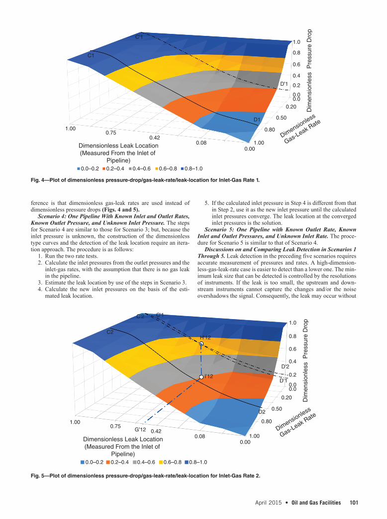
ference is that dimensionless gas-leak rates are used instead of dimensionless pressure drops (Figs. 4 and 5).

Scenario 4: One Pipeline With Known Inlet and Outlet Rates, Known Outlet Pressure, and Unknown Inlet Pressure. The steps for Scenario 4 are similar to those for Scenario 3; but, because the inlet pressure is unknown, the construction of the dimensionless type curves and the detection of the leak location require an itera-tion approach. The procedure is as follows:

1. Run the two rate tests. 2. Calculate the inlet pressures from the outlet pressures and the

inlet-gas rates, with the assumption that there is no gas leak in the pipeline.

3. Estimate the leak location by use of the steps in Scenario 3. 4. Calculate the new inlet pressures on the basis of the esti-

mated leak location.

5. If the calculated inlet pressure in Step 4 is different from that in Step 2, use it as the new inlet pressure until the calculated inlet pressures converge. The leak location at the converged inlet pressures is the solution.

Scenario 5: One Pipeline with Known Outlet Rate, Known Inlet and Outlet Pressures, and Unknown Inlet Rate. The proce-dure for Scenario 5 is similar to that of Scenario 4.

Discussions on and Comparing Leak Detection in Scenarios 1 Through 5. Leak detection in the preceding five scenarios requires accurate measurement of pressures and rates. A high-dimension-less-gas-leak-rate case is easier to detect than a lower one. The min-imum leak size that can be detected is controlled by the resolutions of instruments. If the leak is too small, the upstream and down-stream instruments cannot capture the changes and/or the noise overshadows the signal. Consequently, the leak may occur without



1.0

Dim

ensi

onle

ss P

ress

ure

Dro

p

0.8

0.6

0.4

0.2

0.00.0

0.20

0.50

0.80

D1

1.000.00

0.080.42

0.751.00

0.0–0.2 0.2–0.4 0.4–0.6 0.6–0.8 0.8–1.0


Pipeline)

Dimensionless

Gas-Leak Rate

C'1

D'1

C1

1.0

Dim

ensi

onle

ss P

ress

ure

Dro

p

0.8

0.6

0.4

0.2

0.00.0

0.20

0.50

0.80

D2

1.000.00

0.080.42

0.751.00

0.0–0.2 0.2–0.4 0.4–0.6 0.6–0.8 0.8–1.0


Pipeline)

Dimensionless

Gas-Leak Rate

C'1

H'12

I'12

G'12

C'2

D'1

D'2

C2


notice, or it would be very difficult to identify the leak and to lo-cate the leak point. Generally, the confidence in the level of leak detection in Scenario 1 is higher than that in Scenarios 2 through 5. High-resolution pressure gauges and metering equipment, which can provide high-quality data, are critical to accurate leak detec-tion, especially for Scenarios 2 through 5, in which one of the pres-sures or rates is unknown. It is more difficult to locate leaks in Scenarios 2 through 5. To clearly identify the intersection points (or leak locations) in these scenarios, the difference between Rates 1 and 2 should be as large as possible. It is noted that the selections of Rates 1 and 2 are limited by pipeline operating specifications and the sensitivities of pressure gauges and metering equipment. The shapes of the type curves in Figs. 1 through 5 indicate that it is easier to detect a leak if the leak occurs close to the center of the pipeline. It is also clear that the leak locale can be detected with a higher confidence as the number of flow-rate tests increases. Therefore, three or more rate tests instead of two rate tests can be applied to reduce the uncertainty in leak detection. The rate num-bers required to detect leaks, as mentioned in the preceding, are the minimum numbers required for different scenarios.

Leak Detection in Multiple Pipelines. Scenarios 1 through 5 are for single-pipeline leak detection. It should be noted that gas-trans-portation networks can be complex systems. A gas-transportation network can be considered as a combination of numerous single pipelines and parallel pipelines connected through junctions and/or nodes. Three types of parallel-pipeline setups are shown in Figs. 6, 7, and 8, and are used to illustrate the applications of the pro-posed method to a complicated pipeline system in the field. Most gas-pipeline systems can be decomposed into basic units that are similar to these three setups. If a leak occurs in a pipeline system,

but it is unknown in which pipeline the leak is located, the analysis of the leak in the basic units is a critical step. Therefore, leak detec-tion for parallel pipelines with junctions, as shown in Figs. 6, 7, and 8, is useful from realistic and feasible aspects.

Scenario 6: Parallel-Pipeline Setup, as Shown in Fig. 6. Fig. 6 shows that n parallel pipelines share the same junction upstream. The leak-detection approaches for cases with different given data are described in the following.

Scenario 6A: Known Inlet and Outlet Rates and Pressures. Mul-tiple rate tests are required to identify which pipeline contains the leak. The steps for detecting a leak for each rate test are similar to those in Scenario 1. It should be noted that each pipeline has its own type curves. The pipeline that gives the same leak location under different rates is the one with the leak, while the pipelines that give different leak locations under different rates are excluded.

Scenario 6B: Known Inlet Rate, Known Inlet and Outlet Pres-sures, and Unknown Outlet Rate. For this scenario, multiple rate tests are required. The steps for detecting a leak are similar to those in Scenario 2. The identification of a leaking pipeline is similar to that in Scenario 6A.

Scenario 6C: Known Inlet and Outlet Rates, Known Inlet Pres-sure, and Unknown Outlet Pressure. The steps for detecting a leak are similar to those in Scenario 3. The identification of a leaking pipeline is similar to that in Scenario 6A.

Scenario 6D: Known Inlet and Outlet Rates, Known Outlet Pres-sure, and Unknown Inlet Pressure. The steps for detecting a leak are similar to those in Scenario 4. The identification of a leaking pipeline is similar to that in Scenario 6A.

Scenario 6E: Known Outlet Rate, Known Inlet and Outlet Pres-sures, and Unknown Inlet Rate. The steps for detecting a leak are

Fig. 7—n parallel pipelines share the same junction downstream.

Upstream

Upstream

Upstream Downstream

Pipeline 1

Pipeline n

Pipeline 2

Fig. 6—n parallel pipelines share the same junction upstream.

Upstream

Downstream

Downstream

Downstream

Pipeline 1

Pipeline n

Pipeline 2


similar to those in Scenario 5. The identification of a leaking pipe-line is similar to that in Scenario 6A.

Scenario 7: Parallel-Pipeline Setup, as Shown in Fig. 7. Fig. 7 shows that n parallel pipelines share the same junction down-stream. The leak-detection approaches are similar to those in Sce-narios 6A through 6E.

Scenario 8: Parallel-Pipeline Setup, as Shown in Fig. 8. Fig. 8 shows that n parallel pipelines share the same junctions, both upstream and downstream. Again, the leak-detection approaches are similar to those for Scenarios 6A through 6E.

Identifying Multiple Leaks From a Single Leak in a Pipeline, With Known Inlet and Outlet Pressures and Rates. Leak sce-narios in a gas pipeline were mainly single leaks. Two leak points in the same pipeline were observed in a few field cases. More than two leak points in a pipeline were observed rarely. Assuming flow-rate and pressure data can be measured, multiple rate tests can be used to identify multiple leaks from a single pipeline. If multiple rate tests provide different leak locations, there are two or more leak points. If multiple rate tests result in the same leak location, the leak occurs at a single point. Identifying the leak-point number for two or more leak locations in the same pipeline or multiple leaks in different pipelines connected in a system is very compli-cated and should be the direction of future work.

Field ApplicationThe proposed method was used to detect a leak in an offshore gas pipeline. A 22-in.-diameter, 157.2-km-long pipeline was used to transport gas produced from offshore fields to an onshore terminal. Inlet pressures ranged from 10 to 12 MPa during normal operation, with gas-flow rates varied between 13 and 17 million m3/d. A leak occurred after several years of operation. The inlet-gas-flow rate at the offshore platform was 15.73 million m3/d and the outlet-gas-flow rate at the onshore terminal was 13.92 million m3/d, which means a flow-rate difference of 11.5% between inlet and outlet of the pipe-line. The operator excluded the possibility of a false alarm, con-sidering the high flow-rate difference. The pipeline leak-detection procedure was executed. A leak-detection method that used acoustic technology was selected, and leak detection through launching acoustic pigs was executed. The actual leak detected by physical in-spection occurred 105.354 km away from the inlet of pipeline. The leak location calculated by the proposed method was 105.537 km away, which is close to the actual leak point. This indicated that the proposed method can be used to narrow the range of leak location before the confirmation by physical inspection. The difference be-tween the model and physical detection may be caused by inaccu-rate measurements of temperature, pressure, and flow rate; change in the pipeline inner diameter resulting from scaling, corrosion, and erosion; possible liquid condensed in the pipeline; and inaccurate estimation of gas properties. Therefore, the proposed method can be used to narrow the possible pipeline interval involving the gas leak and reduce the range that will be examined by physical inspection.

Limitations of the Proposed Method and Future-Work RecommendationThe proposed method can detect and evaluate a single leak in a pipeline system. If the gas leak occurs in a pipeline network, the network needs to be decomposed to basic units, as shown in Figs. 6, 7, and 8, before application of the proposed method. However, pipeline networks in operation can be very complicated, and there can be two or more leak points in the same pipeline or different pipelines within the systems. Future work should focus on ex-panding the application of the proposed method to more-compli-cated scenarios, such as multiple leaks in pipeline networks, and experimental tests should be conducted to verify application of the method in such scenarios.

ConclusionsThe following conclusions can be drawn from this study:

• The proposed method provides a straightforward way to lo-cate leaks and estimate leak size.

• The new model can distinguish a single leak from multiple leaks in a single pipeline or parallel pipelines, which is es-sential in selecting appropriate technologies to locate leaks quickly to minimize loss.

• The new method can detect a leak without inlet or outlet flow rate, which cannot be detected by mass-balance approaches.

• The new model can locate a leak point without inlet or outlet pressure. Therefore, it is useful for an offshore or remote/fron-tier pipeline in which pressure data cannot be monitored or transferred in real time.

• We also proposed a method to locate a leak in parallel pipelines, which is critical to leak detection in a gas-pipeline system.

Nomenclature A = cross-sectional area of choke C = constant for unit conversion CD = choke-discharge coefficient Cp = fluid heat capacity at constant pressure Cv = fluid heat capacity at constant volume D = pipe diameter d1 = pipe or tank diameter d2 = choke diameter eD = relative roughness f = friction factor k = Cp/Cv is the specific-heat ratio of fluid L = pipe length Lleak = leak location (measured from the inlet of the pipeline to

the leak locale) Lleak,D = dimensionless leak location MW = molecular weight NRe = Reynolds number p = gas pressure in pipe pdown = downstream pressure

Fig. 8—n parallel pipelines share the same junctions, both upstream and downstream.

Pipeline 1

Pipeline n

Pipeline 2

Upstream Downstream


pinlet = inlet pressure poutlet = outlet pressure ppr = pseudoreduced pressure pup = upstream pressure psc = standard-condition pressure q = gas-flow rate qleak,D = dimensionless gas-leak rate qleak = gas-leak rate qinlet = gas rate at the inlet of the pipeline T = average temperature equal to (Tinlet + Toutlet)/2 Tdown = down temperature Tpr = pseudoreduced temperature Tsc = standard-condition temperature Tup = upstream temperature u = gas-flow velocity z = gas compressibility z = average gas compressibility equal to (zinlet + zoutlet)/2 γg = gas specific gravity ∆pD = dimensionless pressure drop ∆pleak = pressure drop through the pipeline under gas-leak

conditions∆pno leak = pressure drop through the pipeline without gas leak ∆z = outlet elevation minus inlet elevation (note that ∆z is

positive when outlet is higher than inlet) ε = absolute roughness μ = gas viscosity ρ = gas density

AcknowledgmentsThe authors are grateful to the Petroleum Engineering Department at the University of North Dakota. This research is supported in part by the North Dakota Experimental Program to Stimulate Com-petitive Research, under award number EPS-0814442.

ReferencesAnderson, R. and Driscoll, D. 2000. Pathways for Enhanced Integrity, Re-

liability and Deliverability. Report No. DOE/NETL-2000/1130, U.S. Department of Energy: Office of Fossil Energy and the National En-ergy Technology Laboratory, Washington, D.C. (September 2000).

Balda Rivas, K.V. and Civan, F. 2013. Application of Mass Balance and Transient Flow Modeling for Leak Detection in Liquid Pipelines. Pre-sented at the SPE Production and Operations Symposium, Oklahoma City, Oklahoma, USA, 23–26 March. SPE-164520-MS. http://dx.doi.org/10.2118/164520-MS.

Bustnes, T.E., Rousselet, M., and Berland, S. 2011. Leak Detection Per-formance of a Commercial Real Time Transient Model for Troll Oil Pipeline. Presented at the PSIG Annual Meeting, Napa Valley, Cali-fornia, USA, 24–27 May. PSIG-1114.

Eisler, B. 2011. Leak Detection Systems and Challenges for Arctic Subsea Pipelines. Presented at the OTC Arctic Technology Con-ference, Houston, 7–9 February. OTC-22134-MS. http://dx.doi.org/10.4043/22134-MS.

Elliott, J., Fletcher, R., and Wrigglesworth, M. 2008. Seeking the Hidden Threat: Applications of a New Approach in Pipeline Leak Detection. Presented at the Abu Dhabi International Petroleum Exhibition and Conference, Abu Dhabi, 3–6 November. SPE-118070-MS. http://dx.doi.org/10.2118/118070-MS.

Gajbhiye, R.N. and Kam, S.I. 2008. Leak Detection in Subsea Pipeline: A Mechanistic Modeling Approach with Fixed Pressure Boundaries. Presented at the Offshore Technology Conference, Houston, 5–8 May. OTC-19347-MS. http://dx.doi.org/10.4043/19347-MS.

Gonzalez, M.H., Eakin, B.E., and Lee, A.L. 1970. Viscosity of Natural Gases:MonographonAPIResearchProject65. New York: Amer-ican Petroleum Institute.

Guo, B. and Ghalambor, A. 2005. Natural Gas Engineering Handbook, first edition. Houston: Gulf Publishing Company.

Hall, K.R. and Yarborough, L. 1973. A New Equation of State for Z-Factor Calculations. Oil & Gas Journal 71 (25): 82.

Hauge, E., Aamo, O.M., and Godhavn, J.-M. 2009. Model-Based Monitoring and Leak Detection in Oil and Gas Pipelines. SPEProjFac&Const 4 (3): 53–60. SPE-114218-PA. http://dx.doi.org/10.2118/114218-PA.

Huber, D.W. 1981. Real-Time Transient Modem for Batch Tracking, Line Balance and Leak Detection. JCanPetTechnol 20 (3): 46–52. PETSOC-81-03-02. http://dx.doi.org/10.2118/81-03-02.

Jain, A.K. 1976. Accurate Explicit Equation for Friction Factor. Journal of theHydraulicsDivision 102 (5): 674–677.

Luongo, C.A. 1986. An Efficient Program for Transient Flow Simulation in Natural Gas Pipelines. Presented at the PSIG Annual Meeting, New Orleans, 30–31 October. PSIG-8605.

Mactaggart, R.H. 1989. A Sour Gas Leak Detection System Implementa-tion. Presented at the PSIG Annual Meeting, El Paso, Texas, USA, 19–20 October. PSIG-8908.

Massinon, R.V.J. 1988. A Real Time Transient Hydraulic Model for Leak Detection and Batch Tracking on a Liquid Pipeline System. Pre-sented at the Annual Technical Meeting, Calgary, 12–16 June. PETSOC-88-39-93. http://dx.doi.org/10.2118/88-39-93.

Reddy, H.P., Narasimhan, S., and Bhallamudi, S.M. 2006. Simulation and State Estimation of Transient Flow in Gas Pipeline Networks Using a Transfer Function Model. Ind.Eng.Chem.Res. 45 (11): 3853–3863. http://dx.doi.org/10.1021/ie050755k.

Sadovnychiy, S., Bulgakov, I., and Valadez, J. 2005. System for Remote Detection of Pipeline Leakage. Presented at the SPE Latin American and Caribbean Petroleum Engineering Conference, Rio de Janeiro, 20–23 June. SPE-94958-MS. http://dx.doi.org/10.2118/94958-MS.

Schlumberger. 2014. OLGA Dynamic Multiphase Flow Simulator. http://www.software.slb.com/products/foundation/Pages/olga.aspx.

Scott, S.L., Lei, L., and Jinghai, Y. 1999. Modeling the Effects of a Deep-water Leak on Behavior of a Multiphase Production Flowline. Pre-sented at the SPE/EPA Exploration and Production Environmental Conference, Austin, Texas, USA, 1–3 March. SPE-52760-MS. http://dx.doi.org/10.2118/52760-MS.

van der Marel, M. and Sluyter, E.A. 1984. Leak Detection Survey of a 36 Inch Diameter 78 Mile Long Submarine Pipeline. Presented at the SPE Offshore Southeast Asia Show, Singapore, 21–24 February. SPE-12446-MS. http://dx.doi.org/10.2118/12446-MS.

Vrålstad, T., Melbye, A.G., Carlsen, I.M. et al. 2011. Comparison of Leak-Detection Technologies for Continuous Monitoring of Subsea-Production Templates. SPE Proj Fac & Const 6 (2): 96–103. SPE-136590-PA. http://dx.doi.org/10.2118/136590-PA.

Wang, S. and Carroll, J.J. 2007. Leak Detection for Gas and Liquid Pipe-lines by Online Modeling. SPEProjFac&Const 2 (2): 1–9. SPE-104133-PA. http://dx.doi.org/10.2118/104133-PA.

Weymouth, T.R. 1912. Problems in Natural Gas Engineering. Trans ASME 34. Zhou, J. and Adewumi, M.A. 2000. Simulation of transients in natural

gas pipelines using hybrid TVD schemes. Int J Numer MethodsFluids 32 (4): 407–437. http://dx.doi.org/10.1002/(sici)1097-0363 (20000229)32:4<407::aid-fld945>3.0.co;2-9.

Appendix A: Gas Flow in a PipelineGas flow in a nonhorizontal pipeline can be calculated by the Wey-mouth (1912) equation:

qT

p

p e p D

f TzLsc

sc

s

g e

=−( )3 23

2 2 5. inlet outlet

�, ...................................... (A-1)

where

Le L

se

s

=−( )1 ..................................................................... (A-2)

and

sz

Tzg=

0 0375. � � , ................................................................ (A-3)

where q is the gas-flow rate (scf/hr); D is the pipe diameter; e = 2.718; Tsc is the standard-condition temperature; psc is the standard-


condition pressure; pinlet is the inlet pressure; poutlet is the outlet pressure; T is the average temperature equal to (Tinlet + Toutlet)/2; zis the average gas compressibility equal to (zinlet + zoutlet)/2; γg is the gas specific gravity; L is the pipeline length; ∆z is the outlet el-evation minus the inlet elevation (note that ∆z is positive when the outlet is higher than the inlet); and f is the friction factor, which can be calculated by the Jain (1976) correlation:

11 14 2

21 250 9f

eND= − +

. log.

Re.

, ........................................ (A-4)

where eD is the relative roughness, which is defined as the ratio of the absolute roughness to the pipe internal diameter,

eDD = ε , .............................................................................. (A-5)

and NRe is the Reynolds number, which can be expressed as a di-mensionless group,

NDu

Re = �

�, ........................................................................ (A-6)

where ε is the pipe absolute roughness, u is the gas velocity, ρ is the gas density, and μ is the gas viscosity.

Appendix B: Gas-Leak FlowGas leak from the pipeline can be simulated with gas flow through a restriction, such as a nozzle or an orifice, into a lower-pressure environment. Choke performance can be used to evaluate gas flow under this condition. Gas flows through the choke can be divided into subsonic and sonic flows, according to the flow regime. Sonic flow is defined as the point at which the fluid-flow velocity through a choke or throated pipe reaches the sonic velocity in the fluid under the in-situ condition. In other words, the upstream cannot “feel” the pressure wave propagated from downstream upward because the fluid is traveling in the opposite direction with the same velocity under sonic-flow conditions. From its name, we know that subsonic flow exists when flow velocity is less than the sound velocity in the fluid at the in-situ condition, under which the change of downstream pressure can be “felt” by the upstream. Downstream/upstream-pres-sure ratio is used to determine the flow regime. It is expressed as

p

p kc

k

kdown

up

=

+

−2

1

1, .........................................................(B-1)

where pdown is the downstream pressure, pup is the upstream pres-sure, k = Cp/Cv is the specific-heat ratio of fluid, Cp is the fluid heat capacity at constant pressure, and Cv is the fluid heat capacity at con-stant volume.

Sonic flow occurs when the downstream/upstream-pressure ratio is equal to or less than the critical pressure ratio. Otherwise, sub-sonic flow occurs. The gas rate of sonic flow can be calculated by

q C Apk

T kDg

k

k=

+

+−

8792

1

11

upup�

, .................................(B-2)

where A is the cross-sectional area of the choke, CD is the choke-discharge coefficient, Tup is the upstream temperature, and γg is the gas specific gravity.

Under subsonic-flow condition, gas rate is calculated by

q C Apk

k T

p

p

pD

g

k

=−( )

−1 248

2

1

2

, upup

down

up�ddown

upp

k

k

+1

.

.............................................................................................(B-3)

The correlation by Guo and Ghalambor (2005) provides a feasible way to estimate the choke-discharge coefficient:

Cd

d dd

ND = +

+ ( ) −2

1 2

1

0 6

0 31670 025 4

.. log. Re , .........................(B-4)

where d1 is the pipe diameter, d2 is the choke diameter, and NRe is the Reynolds number. The calculations of gas z-factor, density, and viscosity are given in Appendix C.

Appendix C: Gas z-Factor and ViscosityHall and Yarborough (1973) presented an accurate correlation to estimate the z-factor of natural gas. This correlation is summarized as follows:

zAp

Ypr= , .............................................................................(C-1)

where Y is the reduced density to be solved from

Y Y Y Y

YAp BY CYpr

D+ + −−( )

− − + =2 3 4

32

10

and

AT Tpr pr

= − −

0 061251 2 1

12

.exp . ,

BT T Tpr pr pr

= − +14 76 9 76 4 582 3

. . . ,

CT T Tpr pr pr

= − +90 7 242 2 42 42 3

. . . ,

DTpr

= +2 182 82

.. ,

where ppr is the pseudoreduced pressure and Tpr is the pseudo-reduced temperature.

Once gas compressibility factor is provided, gas density can be calculated by

� = 2 728 96

..

M p

zTW . ................................................................(C-2)

With given z-factor and density, gas viscosity can be estimated by use of the correlation by Gonzalez et al. (1970):

� �= ( )−10 4 K X Yexp , ........................................................(C-3a)

KM T

M TW

W

=+( )

+ +9 379 0 01607

209 2 19 26

1 5. .

. .

.

, ........................................(C-3b)

XT

MW= +

+3 448

986 40 01009.

.. , .................................(C-3c)

and

Y X= −2 447 0 2224. . , .......................................................(C-3d)

where MW is the molecular weight.

Kegang Ling is an assistant professor in petroleum engineering at the University of North Dakota. His research interests are in the area of pro-duction optimization. Ling holds a BS degree in geology from the China University of Petroleum, and MS and PhD degrees in petroleum engi-

8 Oil and Gas Facilities • April 2015 April 2015 • Oil and Gas Facilities 9

pinlet = inlet pressure poutlet = outlet pressure ppr = pseudoreduced pressure pup = upstream pressure psc = standard-condition pressure q = gas-flow rate qleak,D = dimensionless gas-leak rate qleak = gas-leak rate qinlet = gas rate at the inlet of the pipeline T = average temperature equal to (Tinlet + Toutlet)/2 Tdown = down temperature Tpr = pseudoreduced temperature Tsc = standard-condition temperature Tup = upstream temperature u = gas-flow velocity z = gas compressibility z = average gas compressibility equal to (zinlet + zoutlet)/2 γg = gas specific gravity ∆pD = dimensionless pressure drop ∆pleak = pressure drop through the pipeline under gas-leak

conditions∆pno leak = pressure drop through the pipeline without gas leak ∆z = outlet elevation minus inlet elevation (note that ∆z is

positive when outlet is higher than inlet) ε = absolute roughness μ = gas viscosity ρ = gas density

AcknowledgmentsThe authors are grateful to the Petroleum Engineering Department at the University of North Dakota. This research is supported in part by the North Dakota Experimental Program to Stimulate Com-petitive Research, under award number EPS-0814442.

ReferencesAnderson, R. and Driscoll, D. 2000. Pathways for Enhanced Integrity, Re-

liability and Deliverability. Report No. DOE/NETL-2000/1130, U.S. Department of Energy: Office of Fossil Energy and the National En-ergy Technology Laboratory, Washington, D.C. (September 2000).

Balda Rivas, K.V. and Civan, F. 2013. Application of Mass Balance and Transient Flow Modeling for Leak Detection in Liquid Pipelines. Pre-sented at the SPE Production and Operations Symposium, Oklahoma City, Oklahoma, USA, 23–26 March. SPE-164520-MS. http://dx.doi.org/10.2118/164520-MS.

Bustnes, T.E., Rousselet, M., and Berland, S. 2011. Leak Detection Per-formance of a Commercial Real Time Transient Model for Troll Oil Pipeline. Presented at the PSIG Annual Meeting, Napa Valley, Cali-fornia, USA, 24–27 May. PSIG-1114.

Eisler, B. 2011. Leak Detection Systems and Challenges for Arctic Subsea Pipelines. Presented at the OTC Arctic Technology Con-ference, Houston, 7–9 February. OTC-22134-MS. http://dx.doi.org/10.4043/22134-MS.

Elliott, J., Fletcher, R., and Wrigglesworth, M. 2008. Seeking the Hidden Threat: Applications of a New Approach in Pipeline Leak Detection. Presented at the Abu Dhabi International Petroleum Exhibition and Conference, Abu Dhabi, 3–6 November. SPE-118070-MS. http://dx.doi.org/10.2118/118070-MS.

Gajbhiye, R.N. and Kam, S.I. 2008. Leak Detection in Subsea Pipeline: A Mechanistic Modeling Approach with Fixed Pressure Boundaries. Presented at the Offshore Technology Conference, Houston, 5–8 May. OTC-19347-MS. http://dx.doi.org/10.4043/19347-MS.

Gonzalez, M.H., Eakin, B.E., and Lee, A.L. 1970. Viscosity of Natural Gases:MonographonAPIResearchProject65. New York: Amer-ican Petroleum Institute.

Guo, B. and Ghalambor, A. 2005. Natural Gas Engineering Handbook, first edition. Houston: Gulf Publishing Company.

Hall, K.R. and Yarborough, L. 1973. A New Equation of State for Z-Factor Calculations. Oil & Gas Journal 71 (25): 82.

Hauge, E., Aamo, O.M., and Godhavn, J.-M. 2009. Model-Based Monitoring and Leak Detection in Oil and Gas Pipelines. SPEProjFac&Const 4 (3): 53–60. SPE-114218-PA. http://dx.doi.org/10.2118/114218-PA.

Huber, D.W. 1981. Real-Time Transient Modem for Batch Tracking, Line Balance and Leak Detection. JCanPetTechnol 20 (3): 46–52. PETSOC-81-03-02. http://dx.doi.org/10.2118/81-03-02.

Jain, A.K. 1976. Accurate Explicit Equation for Friction Factor. Journal of theHydraulicsDivision 102 (5): 674–677.

Luongo, C.A. 1986. An Efficient Program for Transient Flow Simulation in Natural Gas Pipelines. Presented at the PSIG Annual Meeting, New Orleans, 30–31 October. PSIG-8605.

Mactaggart, R.H. 1989. A Sour Gas Leak Detection System Implementa-tion. Presented at the PSIG Annual Meeting, El Paso, Texas, USA, 19–20 October. PSIG-8908.

Massinon, R.V.J. 1988. A Real Time Transient Hydraulic Model for Leak Detection and Batch Tracking on a Liquid Pipeline System. Pre-sented at the Annual Technical Meeting, Calgary, 12–16 June. PETSOC-88-39-93. http://dx.doi.org/10.2118/88-39-93.

Reddy, H.P., Narasimhan, S., and Bhallamudi, S.M. 2006. Simulation and State Estimation of Transient Flow in Gas Pipeline Networks Using a Transfer Function Model. Ind.Eng.Chem.Res. 45 (11): 3853–3863. http://dx.doi.org/10.1021/ie050755k.

Sadovnychiy, S., Bulgakov, I., and Valadez, J. 2005. System for Remote Detection of Pipeline Leakage. Presented at the SPE Latin American and Caribbean Petroleum Engineering Conference, Rio de Janeiro, 20–23 June. SPE-94958-MS. http://dx.doi.org/10.2118/94958-MS.

Schlumberger. 2014. OLGA Dynamic Multiphase Flow Simulator. http://www.software.slb.com/products/foundation/Pages/olga.aspx.

Scott, S.L., Lei, L., and Jinghai, Y. 1999. Modeling the Effects of a Deep-water Leak on Behavior of a Multiphase Production Flowline. Pre-sented at the SPE/EPA Exploration and Production Environmental Conference, Austin, Texas, USA, 1–3 March. SPE-52760-MS. http://dx.doi.org/10.2118/52760-MS.

van der Marel, M. and Sluyter, E.A. 1984. Leak Detection Survey of a 36 Inch Diameter 78 Mile Long Submarine Pipeline. Presented at the SPE Offshore Southeast Asia Show, Singapore, 21–24 February. SPE-12446-MS. http://dx.doi.org/10.2118/12446-MS.

Vrålstad, T., Melbye, A.G., Carlsen, I.M. et al. 2011. Comparison of Leak-Detection Technologies for Continuous Monitoring of Subsea-Production Templates. SPE Proj Fac & Const 6 (2): 96–103. SPE-136590-PA. http://dx.doi.org/10.2118/136590-PA.

Wang, S. and Carroll, J.J. 2007. Leak Detection for Gas and Liquid Pipe-lines by Online Modeling. SPEProjFac&Const 2 (2): 1–9. SPE-104133-PA. http://dx.doi.org/10.2118/104133-PA.

Weymouth, T.R. 1912. Problems in Natural Gas Engineering. Trans ASME 34. Zhou, J. and Adewumi, M.A. 2000. Simulation of transients in natural

gas pipelines using hybrid TVD schemes. Int J Numer MethodsFluids 32 (4): 407–437. http://dx.doi.org/10.1002/(sici)1097-0363 (20000229)32:4<407::aid-fld945>3.0.co;2-9.

Appendix A: Gas Flow in a PipelineGas flow in a nonhorizontal pipeline can be calculated by the Wey-mouth (1912) equation:

qT

p

p e p D

f TzLsc

sc

s

g e

=−( )3 23

2 2 5. inlet outlet

�, ...................................... (A-1)

where

Le L

se

s

=−( )1 ..................................................................... (A-2)

and

sz

Tzg=

0 0375. � � , ................................................................ (A-3)

where q is the gas-flow rate (scf/hr); D is the pipe diameter; e = 2.718; Tsc is the standard-condition temperature; psc is the standard-

106 Oil and Gas Facilities • April 2015 April 2015 • Oil and Gas Facilities PB10 Oil and Gas Facilities • April 2015 April 2015 • Oil and Gas Facilities PB

University of Petroleum, and an MS degree in geology from the Univer-sity of North Dakota.

Peng Pei is a research engineer at the Institute for Energy Studies, Uni-versity of North Dakota. His research interests include energy-related geomechanics and energy-conversion and -utilization processes. Pei has authored or coauthored more than 25 papers. He holds a PhD de-gree in geological engineering and an MS degree in mechanical engi-neering, both from the University of North Dakota.

Jun Ge is a research engineer at the Energy and Environment Research Center (EERC) at the University of North Dakota, where his work focuses on developing geophysical and geomechanical models of the subsurface and running dynamic simulations to determine the long-term fate of produced/injected fluids, including hydrocarbons, CO2, and brine, using oil-and-gas-industry simulation software. Before his position at the EERC, Ge served as an intern at Golder Associates in Redmond, Washington, and as a graduate research assistant at Texas A&M University. His principal areas of interest and expertise include reservoir geomechanics simulation, hydraulic-frac-ture design and propagation modeling, CO2-flooding simulation, numerical modeling of wellbore stability, and rock mechanics applied to petroleum and geothermal reservoir development. Ge has authored or coauthored several publications in the fields of petroleum engineering and geology. He holds an MS degree in petroleum engineering from Texas A&M University; an MS degree in economic geology from Peking University, Bejing; and a BS degree in geology from China University of Geosciences, Wuhan.

neering from the University of Louisiana at Lafayette and Texas A&M University, respectively.

Guoqing Han is an associate professor at China University of Petroleum, Beijing. He has expertise in several fields, including artificial-lift design, flow assurance, and reservoir simulation, in which he has extensive ex-perience in teaching and researching. Han has published more than 20 technical papers. He holds BSc and MSc degrees in process automa-tion and production engineering, respectively, from China University of Petroleum, Shandong. Han also holds a PhD degree in petroleum engi-neering from China University of Petroleum, Beijing.

Xiao Ni is a student in the Petroleum Engineering Department at China University of Petroleum, Beijing. His research interests are in the areas of flow assurance and production optimization. Ni has published sev-eral technical papers.

Chunming Xu is a senior geophysicist at China National Offshore Cor-poration. His research interests are in the areas of reserves evaluation and reservoir characterization. Xu holds a BS degree in geophysics from China Petroleum University.

Jun He is a graduate student at the University of North Dakota. His re-search interests are in the areas of reserves evaluation and reservoir characterization. He holds a BS degree in geology from Southwest Pe-troleum University, an MS degree in petroleum engineering from China

a new method for leak detection in gas pipelines · pdf filea new method for leak detection in...

Documents