a new generation chemical flooding simulator
TRANSCRIPT
A NEW GENERATION CHEMICAL FLOODING SIMULATOR
Final Report for the Period Sept. 2001 - Aug. 2004
Semi-Annual Report for the Period
April1, 2004 – August 30, 2004
by Gary A. Pope, Kamy Sepehrnoori, and Mojdeh Delshad
January 2005
Work Performed under Contract No. DE–FC-26-00BC15314
Sue Mehlhoff, Project Manager U.S. Dept of Energy
National Petroleum Technology Office One West Third Street, Suite 1400
Tulsa, OK 74103-3159
Prepared by Center for Petroleum and Geosystems Engineering
The University of Texas at Austin Austin, TX 78712

ii
DISCLAIMER This report was prepared as an account of work sponsored by an agency of the United States Government. Neither the United States Government nor any agency thereof, nor any of their employees, makes any warranty, express or implied, or assumes any legal liability or responsibility for the accuracy, completeness, or usefulness of any information, apparatus, product, or process disclosed, or represents that its use would not infringe privately owned rights. Reference herein to any specific commercial product, process, or service by trade name, trademark, manufacturer, or otherwise does not necessarily constitute or imply its endorsement, recommendation, or favoring by the United States Government or any agency thereof. The views and opinions of authors expressed herein do not necessarily state or reflect those of the United States Government or any agency thereof.
iii
ABSTRACT The premise of this research is that a general-purpose reservoir simulator for several improved oil recovery processes can and should be developed so that high-resolution simulations of a variety of very large and difficult problems can be achieved using state-of-the-art algorithms and computers. Such a simulator is not currently available to the industry. The goal of this proposed research is to develop a new-generation chemical flooding simulator that is capable of efficiently and accurately simulating oil reservoirs with at least a million gridblocks in less than one day on massively parallel computers. Task 1 is the formulation and development of solution scheme, Task 2 is the implementation of the chemical module, and Task 3 is validation and application. In this final report, we will detail our progress on Tasks 1 through 3 of the project.
iv
TABLE OF CONTENTS DISCLAIMER .................................................................................................................... ii ABSTRACT....................................................................................................................... iii LIST OF TABLES............................................................................................................. vi LIST OF FIGURES .......................................................................................................... vii INTRODUCTION ...............................................................................................................1 EXECUTIVE SUMMARY .................................................................................................4 EXPERIMENTAL...............................................................................................................5 RESULTS AND DISCUSSIONS........................................................................................6
Task 1: Formulation and Development of Solution Scheme .........................................6 Mass Conservation Equation ...................................................................................6 Phase Behavior and Equilibrium Calculations ........................................................8 Phase Stability Analysis...........................................................................................8 Flash Calculation .....................................................................................................9 Phase Identification and Tracking .........................................................................13 Constraints and Constitutive Equations .................................................................15 Physical Property Models ......................................................................................16 Well Model ............................................................................................................19 Overall Computation Procedure of the Simulator .................................................22 Executive Routines in EOSCOMP ........................................................................24 Description of the Solver .......................................................................................25 Solution Approach in Chemical Module ...............................................................26 Non-Orthogonal Grid.............................................................................................26 Approximate Equation ...........................................................................................30 Automatic Time Step Control................................................................................37 Linear and Nonlinear Iterative Solvers ..................................................................38 Enhancements in Well Model................................................................................39 Generation of Derivatives using Automatic Differentiation..................................49
Task 2: Formulation and Implementation of Chemical Module..................................50 Explicit Chemical Module .....................................................................................50 Fully Implicit Chemical Module............................................................................57
Task 3: Validation and Application .............................................................................61 Batch Flash of Ethane-Propylene Binary Mixture.................................................61 Buckley Leverett 1-D Water Flood........................................................................63 Carbon Dioxide Sequestration Case ......................................................................67 Six-Component Compositional Simulation Example............................................70 Chemical Module Tests—Explicit Formulation....................................................79 2-D Surfactant/Polymer Simulation, Case 1..........................................................79 3-D Surfactant/polymer simulation, Case 2...........................................................84 3-D Surfactant/polymer simulation, Case 3...........................................................88 Chemical Module Tests—Fully Implicit Formulation ..........................................90 Parallel Simulations ...............................................................................................98
CONCLUSIONS..............................................................................................................109 REFERENCES ................................................................................................................111
v
NOMENCLATURE ........................................................................................................115 APPENDIX A—Trapping Number Model Calculations Used in the Jacobian ..............120 APPENDIX B—Residuals and Derivation of Jacobian for Newton Iteration ................122
Volume constraint......................................................................................................122 Material Balance Equations .......................................................................................122 Derivatives for Accumulation Term ..........................................................................128 Derivatives for Flux Term .........................................................................................128 Derivatives for Source/Sink Term .............................................................................148
APPENDIX C—Derivations of the Equations in Appendix B........................................151 APPENDIX D—3-D Surfactant/Polymer Input Data......................................................157
vi
LIST OF TABLES Table 1.1—Initial and Injected Gas Composition Used in 3-D Simulations.....................47 Table 3.1—Summary of Input Data for Ethane-Propylene Mixture Batch-Flash
Calculation ...................................................................................................................62 Table 3.2—Comparison of Phase Compositions From GPAS With UTCOMP and
VLMU in Ethane Propylene Batch - Flash Test Case .................................................63 Table 3.3—Comparison of Phase Molar Densities From GPAS With UTCOMP
and VLMU in Ethane Propylene Batch - Flash Test Case...........................................63 Table 3.4—Summary of Input Data for One-Dimensional Buckley Leverett
Problem........................................................................................................................65 Table 3.5—Summary of Input Data For Two Dimensional Carbon Dioxide
Sequestration Problem .................................................................................................68 Table 3.6—Comparison of Mobile Water Phase and Gas Phase Compositions
From GPAS With UTCOMP for Carbon Dioxide Sequestration Problem .................70 Table 3.7—Absolute Differences in Mobile Water Phase and Gas Phase
Compositions From GPAS With UTCOMP for Carbon Dioxide Sequestration Problem After 100 Days ..............................................................................................70
Table 3.8—Summary of Component Critical Properties and Binary Interaction Coefficients for Two-Dimensional Six Component Simulation Example ..................71
Table 3.9—Summary of Input Data for Two-Dimensional Six Component Simulation Example.....................................................................................................72
Table 3.10—Summary of Input Data for Three-Dimensional Six Component Simulation Example.....................................................................................................78
Table 3.11—Input parameters used for Case 1..................................................................80 Table 3.12—Input Parameters for Case 2..........................................................................85 Table 3.13—Input parameters for Case 3 ..........................................................................89
vii
LIST OF FIGURES Figure 1.1—Physical and computational domains. ...........................................................27 Figure 1.2—Metrics evaluation. ........................................................................................29 Figure 1.3—Elemental control volume..............................................................................31 Figure 1.4—Control volume P and its neighbors. .............................................................33 Figure 1.5—Schematic of the grid used in Case 1 simulations. ........................................35 Figure 1.6—Comparison of water production rate using corner point grid
implementation and Cartesian grid. .............................................................................35 Figure 1.7—Comparison of oil production rate using corner point grid
implementation and Cartesian grid. .............................................................................36 Figure 1.8—Schematic of the grid used in Case 2 simulation...........................................36 Figure 1.9—Cumulative water production rate using corner point grid
implementation using the grid shown in Fig. 1.8.........................................................37 Figure 1.10—Cumulative oil production using corner point grid implementation
using the grid shown in Fig. 1.8...................................................................................37 Figure 1.11—Oil production rate comparison between PETSc and TICAMA. ................39 Figure 1.12—Comparison of simulation time for PETSc and TICAMA..........................39 Figure 1.13—Comparison of water production rate for water injection problem
with constant pressure injector and constant rate producer. ........................................44 Figure 1.14—Comparison of oil production rate for water injection problem with
constant pressure injector and constant rate producer. ................................................45 Figure 1.15—Comparison of reservoir pressure for water injection problem with
constant pressure injector and constant rate producer. ................................................45 Figure 1.16—Comparison of water production rate for water injection problem
with constant injection rate and constant pressure producer. ......................................46 Figure 1.17—Comparison of oil production rate for water injection problem with
constant injection rate and constant pressure producer................................................46 Figure 1.18—Comparison of average reservoir pressure for water injection
problem with constant injection rate and constant pressure producer. ........................47 Figure 1.19—Comparison of average reservoir pressure for gas injection problem
with constant injection rate and constant pressure producer. ......................................48 Figure 1.20—Comparison of oil production rate for gas injection problem with
constant injection rate and constant pressure producer................................................48 Figure 1.21—Comparison of gas production rate for gas injection problem with
constant injection rate and constant pressure producer................................................49 Figure 2.1—Flowchart of Newton method for fully implicit chemical flooding
model............................................................................................................................60 Figure 3.1—Oil/water relative permeability curves used in the Buckley Leverett
problem. .......................................................................................................................64 Figure 3.2—Fractional flow curve of water in the Buckley Leverett problem. ................66 Figure 3.3—Comparison of the water saturation profile from GPAS with the
analytical solution and the result from UTCHEM at 0.1, 0.2 and 0.3 pore volumes injected for one-dimensional Buckley Leverett waterflooding problem. .......................................................................................................................66
viii
Figure 3.4—Schematic reservoir geometry (quarter five spot) for the CO2 sequestration problem. .................................................................................................67
Figure 3.5—Comparison of the pressure profile along the x-axis obtained from GPAS with UTCOMP at the end of 100 days for CO2 sequestration problem...........69
Figure 3.6—Comparison of the gas saturation profile along the x-axis from GPAS with UTCOMP at the end of 100 days for the CO2 sequestration problem. ...............69
Figure 3.7—Comparison of the pressure profile along the x-axis from GPAS with UTCOMP at the end of 100 days for the six component problem. .............................73
Figure 3.8—Comparison of the oil saturation profile along the x-axis from GPAS with UTCOMP at the end of 100 days for the six component problem. .....................73
Figure 3.9—Comparison of the gas saturation profile along the x axis from GPAS with UTCOMP at the end of 100 days for the six component problem. .....................74
Figure 3.10—Schematic reservoir geometry for the three dimensional six component simulation case. .........................................................................................75
Figure 3.11—Comparison of the pressure profile along the x-axis from GPAS with UTCOMP for the six component case at the end of two years............................75
Figure 3.12—Comparison of the oil saturation profile along the x-axis from GPAS with UTCOMP for the six component case at the end of two years. ...............76
Figure 3.13—Comparison of the gas saturation profile along the x-axis from GPAS with UTCOMP for the six component case at the end of two years. ...............76
Figure 3.14—Comparison of the average reservoir pressure history from GPAS with UTCOMP for the six component case.................................................................77
Figure 3.15—Comparison of the producer GOR (gas-oil ratio) history of GPAS with UTCOMP result for the six component case. ......................................................77
Figure 3.16—Comparison of produced surfactant concentrations for Case 1...................81 Figure 3.17—Comparison of produced tracer concentration for Case 1. ..........................81 Figure 3.18—Comparison of produced polymer concentration for Case 1.......................81 Figure 3.19—Polymer concentration (GPAS) at Td=0.5 PV. ...........................................82 Figure 3.20—Polymer concentration (UTCHEM) at Td=0.5 PV. ....................................82 Figure 3.21—Surfactant concentration in fluid (GPAS) at Td=0.5 PV.............................82 Figure 3.22—Surfactant concentration in fluid (UTCHEM) at Td=0.5 PV. .....................83 Figure 3.23—Oil saturation profile (UTCHEM) at Td=0.5 PV. .......................................83 Figure 3.24—Oil saturation profile (GPAS) at Td=0.5 PV. ..............................................84 Figure 3.25—Comparison of oil production rate and cumulative oil production for
Case 1...........................................................................................................................84 Figure 3.26—Permeability profile. ....................................................................................85 Figure 3.27—Injection rate and cumulative fluid injected for Case 2...............................86 Figure 3.28—Oil production rate and cumulative oil recovery for Case 2. ......................87 Figure 3.29—Average reservoir pressure for Case 2.........................................................87 Figure 3.30—Surfactant concentration distribution at the end of chemical slug of
0.1 PV. .........................................................................................................................87 Figure 3.31—Oil saturation distribution during post water flush at 0.5 PV......................88 Figure 3.32—Well locations for Case 3. ...........................................................................88 Figure 3.33—Parallel performance speedup for Case 3. ...................................................89 Figure 3.34—Comparison of time spent in solver, Jacobian and MPI
communication for Case 3. ..........................................................................................90
ix
Figure 3.35—Comparison of average reservoir pressure for 1-D surfactant/polymer case. ..............................................................................................91
Figure 3.36—Comparison of water production rate for 1-D surfactant/polymer case...............................................................................................................................91
Figure 3.37—Comparison of oil production rate for 1-D surfactant/polymer case...........91 Figure 3.38—Comparison of surfactant concentration produced for 1-D
surfactant/polymer case. ..............................................................................................92 Figure 3.39—Comparison of tracer concentration for 1-D surfactant/polymer
case...............................................................................................................................92 Figure 3.40—Comparison of polymer concentration for 1-D surfactant/polymer
case...............................................................................................................................92 Figure 3.41—Comparison of average reservoir pressure for 2-D
surfactant/polymer case. ..............................................................................................93 Figure 3.42—Comparison of water production rate for 2-D surfactant/polymer
case...............................................................................................................................94 Figure 3.43—Comparison of oil production rate for 2-D surfactant/polymer case...........94 Figure 3.44—Comparison of surfactant concentration for 2-D surfactant/polymer
case...............................................................................................................................94 Figure 3.45—Comparison of tracer concentration for 2-D surfactant/polymer
case...............................................................................................................................95 Figure 3.46—Comparison of polymer concentration for 2-D surfactant/polymer
case...............................................................................................................................95 Figure 3.47—Comparison of average reservoir pressure for 3-D
surfactant/polymer case. ..............................................................................................96 Figure 3.48—Comparison of water production rate for 3-D surfactant/polymer
case...............................................................................................................................96 Figure 3.49—Comparison of oil production rate for 3-D surfactant/polymer case...........97 Figure 3.50—Comparison of surfactant concentration for 3-D surfactant/polymer
case...............................................................................................................................97 Figure 3.51—Comparison of tracer concentration for 3-D surfactant/polymer
case...............................................................................................................................97 Figure 3.52—Comparison of polymer concentration for 3-D surfactant/polymer
case...............................................................................................................................98 Figure 3.53—GPAS execution time and speedup plots for the case of 77x256x10
using single processor per node. ................................................................................100 Figure 3.54—Speedup curves of each section for the simulation case (77x256x10)
using Myrinet as the interconnect. .............................................................................101 Figure 3.55—Execution time ratio of Fast Ethernet to Myrinet for each sections of
the larger simulation case (77x256x10). ....................................................................101 Figure 3.56—Execution time ratio of single-processor to dual-processor for each
sections of the simulation case (77x256x10) on the cluster with Myrinet. ...............102 Figure 3.57—Well locations for Case 3. .........................................................................103 Figure 3.58—Average reservoir pressure for the parallel surfactant/polymer flood
simulation (96x96x11). ..............................................................................................103 Figure 3.59—Water production rate for the parallel surfactant/polymer flood
simulation (96x96x11). ..............................................................................................104
x
Figure 3.60—Oil production rate for the parallel surfactant/polymer flood simulation (96x96x11). ..............................................................................................104
Figure 3.61—Cumulative oil recovery for the parallel surfactant/polymer flood simulation (96x96x11). ..............................................................................................104
Figure 3.62—Time step for the parallel surfactant/polymer flood simulation (96x96x11).................................................................................................................105
Figure 3.63—Number of Newton iteration for the parallel surfactant/polymer flood simulation (96x96x11)......................................................................................105
Figure 3.64—Average reservoir pressure for the parallel surfactant/polymer flood simulation (384x384x7). ............................................................................................106
Figure 3.65—Total water and oil production rates for the parallel surfactant/polymer flood simulation (384x384x7). ...................................................107
Figure 3.66—Cumulative oil recovery for the parallel surfactant/polymer flood simulation (384x384x7). ............................................................................................107
Figure 3.67—Time step values for the parallel surfactant/polymer flood simulation (384x384x7). ............................................................................................108
Figure 3.68—Number of Newton iterations for the parallel surfactant/polymer flood simulation (384x384x7)....................................................................................108
1
INTRODUCTION Increased oil production using improved oil recovery processes requires numerical modeling of such processes to minimize the risk involved in development decisions. The oil industry is requiring much more detailed analyses with a greater demand for reservoir simulation with geological, physical, and chemical models of much more detail than the past. Reservoir simulation has become an increasingly widespread and important tool for analyzing and optimizing oil recovery projects. Numerical simulation of large petroleum reservoirs with complex recovery processes is computationally challenging due to the problem size and detailed property calculations involved. This problem is compounded by the finer resolution needed to model such processes accurately. Traditionally, such simulations have been performed on workstations or high-end desktop computers. These computers restrict the problem size due to their addressable memory limit and simulation studies of the entire project life become time consuming. Parallel reservoir simulation especially on low cost, high performance computing clusters has alleviated these issues to a certain extent. Recent publications describe the development of such approaches and emphasize the necessity and advantages of using parallel processing (Dogru et al., 2002; Habiballah et al., 2003; Gai et al., 2003; Zhang et al., 2001, Wang et al., 1997). Compositional reservoir simulators which are based on equation of state (EOS) formulations do not handle the modeling of aqueous phase behavior and those which are designed for chemical flood modeling typically assume simplified hydrocarbon phase behavior. There is need to have a single reservoir simulator capable of combining both approaches to benefit from the advantages of both models. The overall objective of this research is to develop such technology using a computational framework that also allows parallel processing. The initial stage of development involved the formulation of a fully implicit, parallel, EOS compositional simulator (Wang et al., 1997). The description of the framework approach used for modular code development and the application to gas injection is given in Wang et al., 1999. Here we report on the implementation of the chemical module to the existing EOS simulator, its validation and application to large-scale chemical flooding simulations. The formulation of the compositional model is first described. The assumptions for the chemical model and its formulation are described next. We use Hand's rule (Hand, 1939) to describe surfactant/oil/brine Type II(-) phase behavior. The trapping number model for relative permeability is implemented to capture the changes in residual saturations caused due to the lowered interfacial tension. The validation of the implementation against the explicit chemical flooding simulator UTCHEM is shown. Application to large-scale problems and tests showing the parallel performance of the simulator are described. With the capability of parallel processing, the general-purpose adaptive simulator (GPAS) can now be used to simulate chemical flooding on a larger scale than before.
2
The need for a reservoir simulation framework that supports and eases physical model development led to the development of the Integrated Parallel Accurate Reservoir Simulator (IPARS) at The University of Texas, Austin (Parashar et al., 1997). The computational framework of IPARS is used to separate the physical reservoir model development from the code involving parallel processing, solvers and other auxiliary functions. The IPARS framework supports three-dimensional multiphase, multicomponent isothermal flow. It has encapsulated functions to perform the input processing, memory allocation and management, domain decomposition, well management, output generation and other functions like table lookups, interpolation, etc. The framework natively supports parallel computation on both distributed and shared memory computers using message passing. On multiprocessor computers, the reservoir domain is divided over the y-direction into several subdomains equal to the number of processors allocated for the run. The computations associated with each of these subdomains are distributed to individual processors. An additional layer of gridblocks is added surrounding each subdomain assigned to a processor. The computational framework provides a routine that updates data in this communication layer to enable each processor to perform its calculations while communicating necessary data with the other processors using the message passing interface (MPI). The primary source of the solvers used in the framework is that provided by the software package called PETSc (Portable Extensible Toolkit for Scientific Computation) (Balay et al., 1997). Other solvers based on the Generalized Minimum Residual Method (GMRES), Line Successive Over-relaxation (LSOR) and Pre-conditioned Conjugate Gradient (PCG) methods have also been implemented as additional options in the framework. All of these solvers provide the users great flexibility and control of the numerical methods used for the solutions. Finite difference formulations with a block-centered grid are used in the framework. The nonlinear difference equations are solved by either fully implicit or semi-implicit techniques. Both mass balance and volume balance is supported. Since the portability of the simulator is very important, FORTRAN 77 is used wherever possible. For memory management and user interaction, classical C is used. Commercial libraries are prohibited except in the graphics front end to the simulator. The simulator is formulated for a distributed memory, message passing machine. Free-format keyword input is used for direct data input. The simulator uses a single set of units to solve the partial differential equations. However, the user may choose any physically correct units for the input variables and they will then be converted to the default internal unit using appropriate conversion factor. The overall structure of IPARS framework consists of 3 layers:
• Executive layer that consists of routines that direct the overall course of the simulation
• Work routines that are typically FORTRAN subroutines that perform grid element computations.

3
• Data-management layer that handles the distribution of grid across processing nodes, local storage allocation, dynamic reallocation and dynamic load balancing, and communication rescheduling. The data-management layer is also responsible for checkpoint/restart, input/output and visualization.
The fully implicit EOS compositional formulation has already been implemented into the IPARS framework and successfully tested. The Peng-Robinson EOS is used for hydrocarbon phase behavior calculations. The linear solvers from PETSc package are used for the solution of underlying linear equations. The framework provides hooks for implementing specific physical models. Such hooks bridge the models with the framework. There are several executive routines, and any communications between the processors and compositional model are performed in these routines. Many tests have been performed using the EOS compositional simulator on variety of computer platforms such as IBM SP and a cluster of PCs (Wang et al., 1999; Uetani et al., 2002). The goal of this project was to add a chemical module to the existing compositional Peng-Robinson cubic equation of state (EOS). The simulator called GPAS, General Purpose Adaptive Reservoir Simulator, will then include the IPARS framework, and the compositional and chemical modules. We detail our progress on Tasks 1 through 3 throughout the three-year project. We have formulated the mass conservation equation and physical properties for chemical species such as tracers, polymer, surfactant and electrolytes. We implemented and validated the chemical module. The chemical module was added both using a hybrid approach and also a fully implicit formulation. We have verified and validated the formulation and the implementation in GPAS by making comparison with analytical solutions of the known problem, with other reservoir simulators such as UTCHEM, UTCOMP, and Eclipse. We have also conducted a series of benchmarks by running the General Purpose Adaptive (GPAS) simulator on a Linux cluster and studied the scalability while using different interconnects. The results were very encouraging and indicated that GPAS performance scales linearly from one to 64 single processor nodes using a low latency, high-bandwidth such as Myrinet. The progress in the last six months of the project was on addition of more flexible corner point grid geometry and also the implementation of the fully implicit surfactant and its properties. We performed a series of validation tests to compare the simulation results accuracy and efficiency of the explicit and fully implicit chemical modules.
4
EXECUTIVE SUMMARY The premise of this research is that a general-purpose reservoir simulator for several improved oil recovery processes can and should be developed so that high-resolution simulations of a variety of very large and difficult problems can be achieved using state-of-the-art algorithms and computers. Such a simulator is not currently available to the industry. The goal of this proposed research is to develop a new-generation chemical flooding simulator that is capable of efficiently and accurately simulating oil reservoirs with at least a million gridblocks in less than one day on massively parallel computers. Task 1 is the formulation and development of solution scheme, Task 2 is the implementation of the chemical module, and Task 3 is validation and application. We made significant progress on all three tasks and we were on schedule on both technical and budget. In this report, we will detail our progress on Tasks 1 through 3 of the project. We report on the implementation of the chemical module to the existing EOS simulator, its validation and application to large-scale chemical flooding simulations. The formulation of the compositional model is first described. The assumptions for the chemical model and its formulation are described next. The aqueous species added as part of the chemical model are surfactant, polymer, electrolytes, and tracers. We use Hand's rule (Hand, 1939) to describe surfactant/oil/brine Type II(-) phase behavior. The trapping number model for relative permeability is implemented to capture the changes in residual saturations caused due to the lowered interfacial tension. The validation of the implementation against the explicit chemical flooding simulator UTCHEM is shown. Application to large-scale problems and tests showing the parallel performance of the simulator are described. We have implemented the chemical module using both explicit and fully implicit formulations. The explicit approach we used to couple the models is easy to implement, computationally efficient and extendable to many other interesting reservoir problems involving aqueous chemistry. With the fully implicit formulation we can take advantage of large time steps. We have also added a corner point grid geometry option for modeling more complex reservoir geometries. With the capability of parallel processing, the general-purpose adaptive simulator (GPAS) can now be used to simulate chemical flooding on a larger scale than before. We have also conducted a series of benchmarks by running GPAS on Xeon-bases Linux cluster and studied the scalability while using different interconnects for the cluster. The simulations were performed for a gas injection process in a reservoir with 197,120 gridblocks and total of 88 wells in a staggered line drive pattern. The speed up results indicated a very good performance. The GPAS showed the best performance as well as scalability (speedup) on a cluster with Myrint.

5
EXPERIMENTAL This project does not include an experimental task.
6
RESULTS AND DISCUSSIONS
Task 1: Formulation and Development of Solution Scheme The effort on this task was directed towards the formulation of tracer, polymer, electrolytes, and surfactant species in GPAS. We implemented the aqueous species using both explicit and fully implicit methods. The explicit formulation was based on a hybrid approach where the mass conservation equations for hydrocarbon species are solved implicitly where the aqueous species mass balances are solved explicitly using an updated phase fluxes, saturations, and densities. To take advantage of the larger time steps with the fully implicit formulation to reduce the simulation time, we have developed a fully implicit module of chemical flood with the relevant physical properties. The advantage of the hybrid method is in the fast and easy implementation of the physical models. For completeness, we first give a review of the mathematical formulation of the compositional model.
Mass Conservation Equation The assumptions made in developing the formulation are:
• Reservoir is isothermal. • Darcy's law describes the multiphase flow of fluids through the porous media. • Impermeable zones represented by the no-flow boundaries surround the reservoir. • The injection and production of fluids are treated as source or sink terms. • The rock is slightly compressible and immobile. • Each hydrocarbon phase is composed of nc hydrocarbon components, which may
include the non-hydrocarbon components such as CO2, N2 or H2S. • Instantaneous local thermodynamic equilibrium between hydrocarbon phases. • Negligible capillary pressure effects on hydrocarbon phase equilibrium. • Water is slightly compressible and water viscosity is constant.
The general mass conservation equation for species i in a volume V can be expressed as
c
Rate of accumulation of i in V
Rate of i transported into V
Rate of i transported from V
Rate of production of i in V ,i 1, , N
=
−
+ = …
(1.1)
The differential form for the species conservation equation can be expressed as:
7
ii i
WN R 0
t∂
+ ∇ • − =∂
(1.2)
where Wi is the overall concentration of i in units of mass of i per unit bulk volume, iN is the flux vector of species i in units of mass of i per surface area-time and Ri is the mass rate of production in units of mass of i per bulk volume-time. The mass balance equation can be expressed in terms of moles per unit time by defining each term of Eq. 1.2 in terms of the porous media and fluid properties such as porosity, permeability, density, saturations, compositions, rates etc. The accumulation term for a porous medium becomes
pn
i j j ijj 1
W S x=
= φ ξ∑ (1.3)
where φ is the porosity, jξ is the molar density of phase j, Sj is the saturation of phase j and xij is the mole fraction of component i in phase j. The flux vector of component i is a sum of the convective and the dispersive flux, and can be expressed as
pn
j ij j j j ij ijj 1
N x u S K x=
= ξ − φξ • ∇∑ (1.4)
where ju represents the superficial velocity or flux of phase j. The flux is evaluated using the Darcy's law for multiphase flow of fluids through porous media.
j rj j ju K ( P D)= − λ ∇ − γ ∇ (1.5) Darcy's law is a fundamental relationship describing the flow of fluids in permeable media under laminar flow conditions. The differential form of Darcy's law can be used to treat multiphase unsteady state flow, non-uniform permeability, non-uniform pressure gradients. It is used to govern the transport of phases from one cell to another under the local pressure gradient, rock permeability, relative permeability and viscosity. Converting each of the terms in the mass balance equation to units of moles per unit time and expressing the flux using Darcy's law, the mass balance for each component i is the following partial differential equation:
p pn ni
j j ij j j ij j j j j ij ijbj 1 j 1
qS x x ( P D) S K x 0
t V= =
∂ φ ξ + ∇ • ξ λ ∇ − γ ∇ + φξ • ∇ − = ∂
∑ ∑ (1.6)
8
Multiplying both sides of Eq. 1.6 by Vb gives
p pn n
b j j ij b j j ij j j j j ij ij ij 1 j 1
c
V S x V x ( P D) S K x q 0t
for i 1, ,n
= =
∂ φ ξ − ∇ • ξ λ ∇ − γ ∇ + φξ • ∇ − = ∂
=
∑ ∑
…
(1.7)
The above equation is written is terms of moles per unit time, in which qi is the molar injection (positive) or production (negative) rate for component i. The mobility for phase j is defined as
rjj
j
kkλ =
µ (1.8)
The physical dispersion term has not yet been implemented in GPAS.
Phase Behavior and Equilibrium Calculations The phase equilibrium relationship determines the number, amounts and compositions of all the equilibrium phases. The sequence of phase equilibrium calculations is as follows:
1. The number of phases in a gridblock is determined using the phase stability analysis.
2. After the number of phases is determined, the composition of each equilibrium phase is determined.
3. The phases in the gridblock are tracked for the next time step calculations.
Phase Stability Analysis The stability algorithm has not been implemented in Equation of State Compositional Model (EOSCOMP). One way of doing the phase stability analysis was given by Michelsen (1982). The Michelsen's approach could be used for the implementing the phase stability analysis in EOSCOMP as explained below. A stability analysis on a mixture of overall hydrocarbon composition Z is a search for a trial phase, taken from the original mixture that, when combined with the remainder of the mixture, gives a value of Gibbs free energy that is lower than a single-phase mixture of overall hydrocarbon composition, Z (Michelsen, 1982; Trangenstein, 1987; Chang, 1990). If such a search is successful, an additional phase must be added to the phase equilibrium calculation. This condition is expressed mathematically as
9
cn
i i ii 1
G y (Y) (Z)=
∆ = µ − µ ∑ (1.9)
where iµ is the chemical potential of component i and yi is the mole fraction of component i in the trial phase. Thus, if for any set of mole fractions the value of G∆ at constant temperature and pressure is greater than zero, then the phase will be stable. If a composition can be found such that G 0∆ < , the phase will be unstable. The phase stability analysis is to solve the following set of nonlinear equations for the variables Yi
i i i cln Y ln (Y) h 0 for i 1, , n+ φ − = = … (1.10) where the mole fraction Y and hi is related to these variables by
ci
i n
si 1
Yy
Y=
=
∑ (1.11)
i i i ch ln Z ln (Z) for i 1, , n= + φ = … (1.12)
Flash Calculation Once a mixture has been shown to split into more than one phase by the stability calculation, the flash involves calculation of the mole fraction and composition of each phase at the given temperature, pressure and overall composition of the fluid. The governing equations for the flash require equality of component fugacities and mass balance. The equilibrium solution must satisfy three conditions:
• Mass conservation of each component in the mixture • Chemical potentials for each component are equal in all phases • Gibbs free energy at constant temperature and pressure is a minimum
Fugacity is calculated using the Peng Robinson equation-of-state. The phase composition constraint, which states that the sum of the mole fraction of all the components in a phase equals to one, and the Rachford-Rice equation for determining the phase amounts for two hydrocarbon phases are implicitly used in the solution of the fugacity equation. The Rachford-Rice equation is used to determine the phase compositions and amounts. This equation requires the values of the equilibrium ratios Ki, which are defined as the ratio of the mole fractions of component i in oil and gas phases, respectively. The Ki values are determined by the equality of component fugacities in each phase. The fugacity equality,
10
the Rachford-Rice equation and the Peng Robinson equation of state are described below in detail.
Equality of the Component Fugacity One of the criteria for phase equilibrium is the equality of the partial molar Gibbs free energies or the chemical potentials. Alternatively, this criterion can be expressed in terms of fugacity (Sandler, 1999): with the assumption of local thermodynamic equilibrium for the hydrocarbon phases, the criterion of phase equilibrium applies (Smith and Van Ness, 1975), namely
ij i c pf f for i 1, , n and j 2, , n ( j )= = = ≠… … (1.13) where phase has been chosen as a reference phase. The fugacity of a component in a phase is taken as a function of pressure and phase composition, at a given temperature,
( )ij ij j c pf f P, x for i 1, , n and j 2, , n ( j )= = = ≠… … (1.14)
Composition Constraint The phase composition constraint is
cn
iji 1
x 1 0=
− =∑ (1.15)
where the mole fractions are defined as
ijij c p
j
nx for i 1, , n and j 2, , n
n= = =… … (1.16)
Rachford-Rice Equation In a classical flash calculation, the amount and composition of each equilibrium phase is evaluated using a material-balance equation after each update of the K-value from the equation-of-state:
cni i
ii 1
(K 1)Zr(v) 0
1 v(K 1)=
−= =
+ −∑ (1.17)
where v is the mole fraction of gas in absence of water, Ki is the equilibrium ratio, Zi is the overall mole fraction of component i in the feed and r(v) is the residual of the Rachford-Rice equation.
11
The component mole fractions in the liquid and gas phases are then computed from the equations:
ii
i
Zx
1 v(K 1)=
+ − (1.18)
i i
ii
Z Ky
1 v(K 1)=
+ − (1.19)
The range for v is defined by
lmax
rmin
1v 01 K
1v 01 K
= <−
= >−
(1.20)
Equation 1.17 is a monotonically decreasing function of v with asymptotes at v1 and vr. Usually, a Newton iteration can efficiently solve Eqs. 1.18 and 1.19 forv. However, round-off errors occur when solving Eq. 1.17.
Leibovici and Neoschil Equation EOSCOMP solves the Rachford-Rice Equation. As was described above, round-off errors occur when solving the Rachford-Rice equation. To avoid the round off errors that occur when solving Eq. 1.17, the original Rachford-Rice equation can be changed into a form that is more nearly linear with respect to v as done by Leibovici and Neoschil (1992) and this approach could be implemented in EOSCOMP. The Leibovici and Neoschil equation is given by
cni i
l rii 1
(K 1)Zr(v) (v v )(v v) 01 v(K 1)=
−= − − =
+ −∑ (1.21)
The range for v is defined by
i imin i i
i
Z K 1v max for K 1 and Z 0
K 1 −
= > < − (1.22)
imax i i
i
Z 1v min for K 1 and Z 0
K 1 −
= < > − (1.23)
Also, the Newton procedure is used to solve Eq. 1.21 for v.
12
Equation of State The Peng Robinson equation of state (Peng and Robinson, 1976) is
RT a(T)PV b V(V b) b(V b)
= −− + + −
(1.24)
The parameters a and b for a pure component are computed from
2 2c
c
R Ta(T) 0.45724 (T)
P= α (1.25)
c
T1 1T
α = + κ −
(1.26)
c
c
RTb 0.07780
P= (1.27)
20.37464 1.54226 0.26992 if 0.49κ = + ω − ω ω < (1.28)
2 3 0.379640 + 1.485030 - 0.164423 + 0.016666 if 0.49κ = ω ω ω ω ≥ (1.29)
For a multi component mixture, the mixing rules for the two parameters are
c c
c
N N
i j i j iji 1 j 1N
i ii 1
a x x a a (1 k )
b x b
= =
=
= −
=
∑ ∑
∑ (1.30)
where for component i, the ai is computed from Eq. 1.25, and bi is computed from Eq. 1.27. The constant, kij is called the binary interaction coefficient between components i and j. The Peng Robinson Equation of state can be written in the form
3 2Z Z Z 0+ α + β + γ = (1.31)
where PVZRT
= is the compressibility factor, and the parameters are expressed as
13
1 Bα = − + (1.32)
2A 3B 2Bβ = − − (1.33)
2 3AB B Bγ = − + + (1.34)
2aPA
(RT)= (1.35)
bPBRT
= (1.36)
In GPAS, the equation-of-state calculations are done in the subroutine named XEOS, which contains the four subroutines EOSPURE, EOSMIX, EOSPHI and EOSPARTIAL. The equation-of-state parameters for each pure component are calculated in the subroutine EOSPURE. Mixture values are calculated in the subroutine EOSMIX. The fugacity coefficient is calculated from the equation-of-state in the subroutine EOSPHI and the equation-of-state related derivatives are computed in the EOSPARTIAL subroutine. The subroutine EOSCUB solves the Peng Robinson cubic equation-of-state and calculates the compressibility factor and its derivative. EOSCOMP requires the pure component critical temperature, critical pressure, critical volume, acentric factors, molecular weights and binary interaction coefficients to calculate the equation of state parameters. The volume shift parameter is not implemented in GPAS. The main flash subroutine in GPAS is XFLASH. This subroutine performs the flash calculation at a given initial composition, temperature and pressure. The number of components, binary interaction coefficients and the equilibrium ratio values are also part of the input to this subroutine. An initial estimate of the equilibrium values is done in the subroutine STABL, which is then passed to the flash calculations. The flash subroutine calculates the liquid and vapor phase mole fractions, liquid and vapor compressibility factors, and also the negative residual of component i in cell k . The subroutine SOLVE solves the Rachford-Rice equation for finding the phase composition and the phase amounts.
Phase Identification and Tracking Phase identification deals with the labeling of a phase as oil, gas, or aqueous phase at the initial conditions and also when a new phase appears. After a phase has been identified, phase tracking does the labeling of a phase during the simulation. Labeling phases consistently is important because of the need to assign a consistent relative permeability to each phase during a numerical simulation. Perschke (1988) developed a method for the phase identification and tracking in which both phase mass density and phase composition are used. This is the procedure followed in GPAS. Once a phase has been

14
identified, it is tracked during simulation by comparing the mole fraction value of a selected or key component in the equilibrium phases at the new time step with the values at the old time step. The phases at the new time step are labeled such that the mole fraction values are closest to the values at the old time step. The algorithm used in GPAS for naming a phase when the hydrocarbon mixture is a single phase is similar to that proposed by Gosset et al. (1986). The parameters A and B of a two-parameter cubic EOS are computed from
2c
a2 2c
PTaPA(RT) P T
= = Ω α (1.37)
c
bc
PTbPBRT P T
= = Ω (1.38)
where
a 0.4572355299Ω =
b 0.077796074Ω = Dividing Eq. 1.37 by Eq. 1.38 gives:
a c
b
TAB T
Ω= α
Ω (1.39)
where α is defined in Eq. 1.26. A fluid is assumed to be in single-phase if cT T> , which also implies 1α ≤ . From Eq. 1.39 this implies
a
b
AB
Ω≤
Ω (1.40)
or its molar volume to be greater than the critical molar volume, cv v> , which implies
c
b
BZZ >
Ω (1.41)
In GPAS, the subroutine EOS_1PH identifies a single phase as oil or gas using the above method. Also, an option is provided in the code to identify a single phase by the
15
conventional method: The fluid is liquid when sum of i iZ K 1= , and the fluid is gas when the sum of i iZ / K 1= .
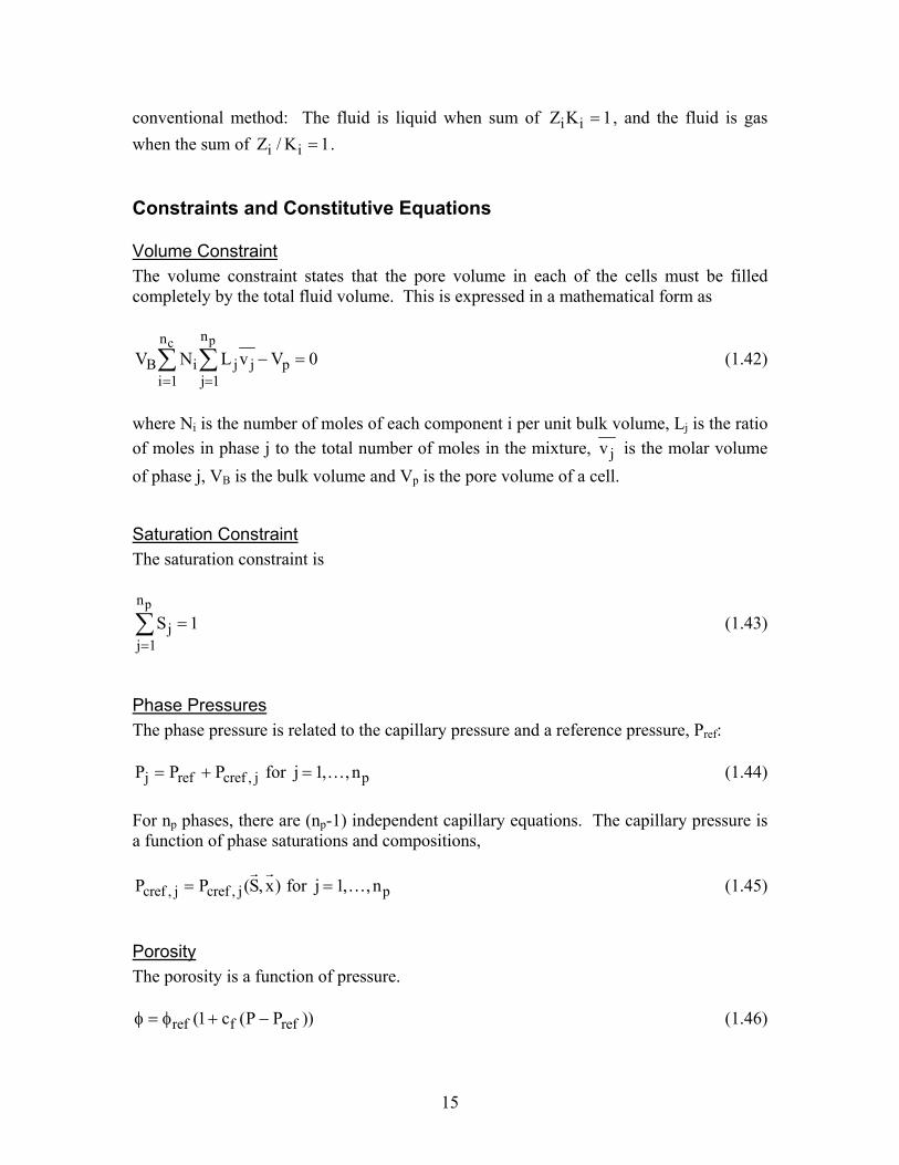
Constraints and Constitutive Equations
Volume Constraint The volume constraint states that the pore volume in each of the cells must be filled completely by the total fluid volume. This is expressed in a mathematical form as
pc nn
B i j j pi 1 j 1
V N L v V 0= =
− =∑ ∑ (1.42)
where Ni is the number of moles of each component i per unit bulk volume, Lj is the ratio of moles in phase j to the total number of moles in the mixture, jv is the molar volume of phase j, VB is the bulk volume and Vp is the pore volume of a cell.
Saturation Constraint The saturation constraint is
pn
jj 1
S 1=
=∑ (1.43)
Phase Pressures The phase pressure is related to the capillary pressure and a reference pressure, Pref:
j ref cref , j pP P P for j 1, , n= + = … (1.44) For np phases, there are (np-1) independent capillary equations. The capillary pressure is a function of phase saturations and compositions,
cref , j cref , j pP P (S, x) for j 1, , n= = … (1.45)
Porosity The porosity is a function of pressure.
ref f ref(1 c (P P ))φ = φ + − (1.46)
16
where φref is the porosity at the reference pressure, Pref and φ is calculated at the pressure P. In GPAS, the porosity calculation is performed in the subroutine AQUEOUS. The AQUEOUS subroutine also calculates the aqueous phase molar and mass densities.
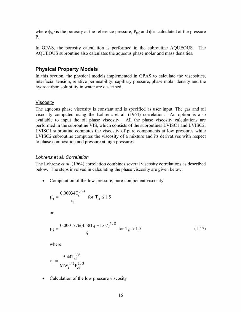
Physical Property Models In this section, the physical models implemented in GPAS to calculate the viscosities, interfacial tension, relative permeability, capillary pressure, phase molar density and the hydrocarbon solubility in water are described.
Viscosity The aqueous phase viscosity is constant and is specified as user input. The gas and oil viscosity computed using the Lohrenz et al. (1964) correlation. An option is also available to input the oil phase viscosity. All the phase viscosity calculations are performed in the subroutine VIS, which consists of the subroutines LVISC1 and LVISC2. LVISC1 subroutine computes the viscosity of pure components at low pressures while LVISC2 subroutine computes the viscosity of a mixture and its derivatives with respect to phase composition and pressure at high pressures.
Lohrenz et al. Correlation The Lohrenz et al. (1964) correlation combines several viscosity correlations as described below. The steps involved in calculating the phase viscosity are given below:
• Computation of the low-pressure, pure-component viscosity
0.94ri
i rii
0.00034Tfor T 1.5µ = ≤
ς
or
5 / 8
rii ri
i
0.0001776(4.58T 1.67)for T 1.5
−µ = >
ς (1.47)
where
1/ 6ci
i 1/ 2 2 / 3i ci
5.44T
MW Pς =
• Calculation of the low pressure viscosity
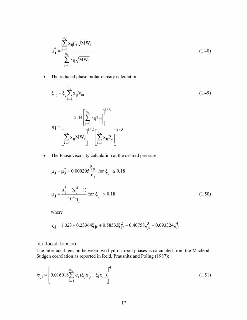
17
c
c
n
ij i i* i 1j n
ij ii 1
x MW
x MW
=
=
µ
µ =∑
∑ (1.48)
• The reduced phase molar density calculation
cn
j ij cijri 1
x V=
ξ = ξ ∑ (1.49)
c
c c
1/ 6n
ij cii 1
j 1/ 2 2 / 3n n
ij i ij cii 1 i 1
5.44 x T
x MW x P
=
= =
η =
∑
∑ ∑
• The Phase viscosity calculation at the desired pressure
jr*j j jr
j0.000205 for 0.18
ξµ = µ + ξ ≤
η
* 4j j
j jr4j
( 1)for 0.18
10
µ + χ −µ = ξ >
η (1.50)
where 2 3 4
j jr jr jrjr1.023 0.23364 0.58533 0.40758 0.093324χ = + ξ + ξ − ξ + ξ
Interfacial Tension The interfacial tension between two hydrocarbon phases is calculated from the Macleod-Sudgen correlation as reported in Reid, Prausnitz and Poling (1987):
c4n
jl i j ij l ili 1
0.016018 ( x x )=
σ = ψ ξ − ξ
∑ (1.51)
18
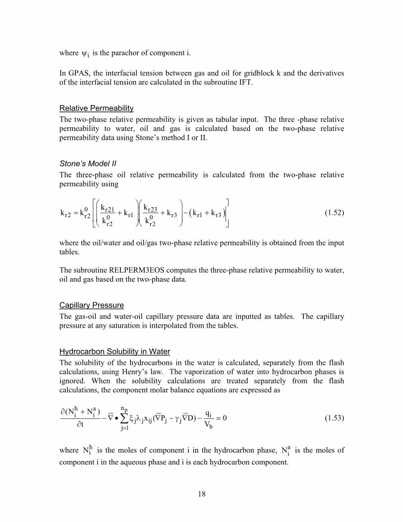
where iψ is the parachor of component i. In GPAS, the interfacial tension between gas and oil for gridblock k and the derivatives of the interfacial tension are calculated in the subroutine IFT.
Relative Permeability The two-phase relative permeability is given as tabular input. The three -phase relative permeability to water, oil and gas is calculated based on the two-phase relative permeability data using Stone’s method I or II.
Stone’s Model II The three-phase oil relative permeability is calculated from the two-phase relative permeability using
( )0 r23r21r2 r1 r3 r1 r3r2 0 0
r2 r2
kkk k k k k k
k k
= + + − +
(1.52)
where the oil/water and oil/gas two-phase relative permeability is obtained from the input tables. The subroutine RELPERM3EOS computes the three-phase relative permeability to water, oil and gas based on the two-phase data.
Capillary Pressure The gas-oil and water-oil capillary pressure data are inputted as tables. The capillary pressure at any saturation is interpolated from the tables.
Hydrocarbon Solubility in Water The solubility of the hydrocarbons in the water is calculated, separately from the flash calculations, using Henry’s law. The vaporization of water into hydrocarbon phases is ignored. When the solubility calculations are treated separately from the flash calculations, the component molar balance equations are expressed as
pnh ai i i
j j ij j jbj 1
(N N ) qx ( P D) 0
t V=
∂ +− ∇ • ξ λ ∇ − γ ∇ − =
∂ ∑ (1.53)
where h
iN is the moles of component i in the hydrocarbon phase, aiN is the moles of
component i in the aqueous phase and i is each hydrocarbon component.
19
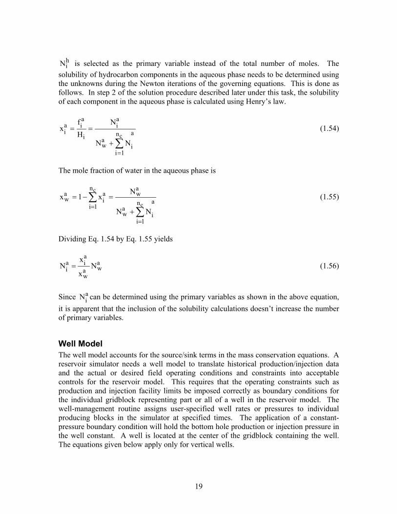
hiN is selected as the primary variable instead of the total number of moles. The
solubility of hydrocarbon components in the aqueous phase needs to be determined using the unknowns during the Newton iterations of the governing equations. This is done as follows. In step 2 of the solution procedure described later under this task, the solubility of each component in the aqueous phase is calculated using Henry’s law.
c
a aa i ii ani a
w ii 1
f Nx
HN N
=
= =
+ ∑ (1.54)
The mole fraction of water in the aqueous phase is
c
c
n aa a ww i ani 1 a
w ii 1
Nx 1 x
N N=
=
= − =
+
∑∑
(1.55)
Dividing Eq. 1.54 by Eq. 1.55 yields
aa ai
wi aw
xN N
x= (1.56)
Since a
iN can be determined using the primary variables as shown in the above equation, it is apparent that the inclusion of the solubility calculations doesn’t increase the number of primary variables.
Well Model The well model accounts for the source/sink terms in the mass conservation equations. A reservoir simulator needs a well model to translate historical production/injection data and the actual or desired field operating conditions and constraints into acceptable controls for the reservoir model. This requires that the operating constraints such as production and injection facility limits be imposed correctly as boundary conditions for the individual gridblock representing part or all of a well in the reservoir model. The well-management routine assigns user-specified well rates or pressures to individual producing blocks in the simulator at specified times. The application of a constant-pressure boundary condition will hold the bottom hole production or injection pressure in the well constant. A well is located at the center of the gridblock containing the well. The equations given below apply only for vertical wells.
20
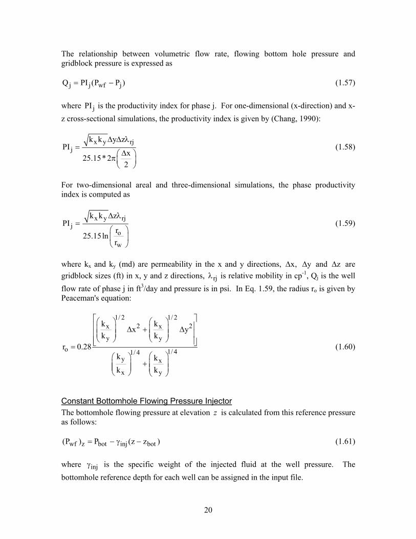
The relationship between volumetric flow rate, flowing bottom hole pressure and gridblock pressure is expressed as
j j wf jQ PI (P P )= − (1.57) where jPI is the productivity index for phase j. For one-dimensional (x-direction) and x-z cross-sectional simulations, the productivity index is given by (Chang, 1990):
x y rjj
k k y zPI
x25.15* 22
∆ ∆ λ=
∆ π
(1.58)
For two-dimensional areal and three-dimensional simulations, the phase productivity index is computed as
x y rjj
o
w
k k zPI
r25.15ln
r
∆ λ=
(1.59)
where kx and ky (md) are permeability in the x and y directions, x,∆ y∆ and z∆ are gridblock sizes (ft) in x, y and z directions, rjλ is relative mobility in cp-1, Qj is the well flow rate of phase j in ft3/day and pressure is in psi. In Eq. 1.59, the radius ro is given by Peaceman's equation:
1/ 2 1/ 22 2x x
y yo 1/ 41/ 4
y x
x y
k kx y
k kr 0.28
k kk k
∆ + ∆ =
+
(1.60)
Constant Bottomhole Flowing Pressure Injector The bottomhole flowing pressure at elevation z is calculated from this reference pressure as follows:
wf z bot inj bot(P ) P (z z )= − γ − (1.61) where injγ is the specific weight of the injected fluid at the well pressure. The bottomhole reference depth for each well can be assigned in the input file.
21
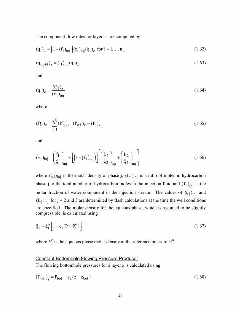
The component flow rates for layer z are computed by
i z 1 inj i inj t z c(q ) 1 (f ) (z ) (q ) for i 1, , n = − = … (1.62)
cn 1 z 1 inj t z(q ) (f ) (q )+ = (1.63) and
t zt z
t inj
(Q )(q )
(v )= (1.64)
where
pn
t z j z wf z j zj 1
(Q ) (PI ) (P ) (P )=
= − ∑ (1.65)
and
( )( )1 2 2t inj 1 inj
1 2 2inj inj inj
f L L(v ) 1 f
= + − + ξ ξ ξ (1.66)
where j inj( )ξ is the molar density of phase j, j inj(L ) is a ratio of moles in hydrocarbon
phase j to the total number of hydrocarbon moles in the injection fluid and ( )1 injf is the
molar fraction of water component in the injection stream. The values of j inj( )ξ and
j inj(L ) for j = 2 and 3 are determined by flash calculations at the time the well conditions are specified. The molar density for the aqueous phase, which is assumed to be slightly compressible, is calculated using
o o1 11 11 c (P P ) ξ = ξ + − (1.67)
where o
1ξ is the aqueous phase molar density at the reference pressure o1P .
Constant Bottomhole Flowing Pressure Producer The flowing bottomhole pressures for a layer z is calculated using ( )wf bot z botzP P (z z )= − γ − (1.68)
22
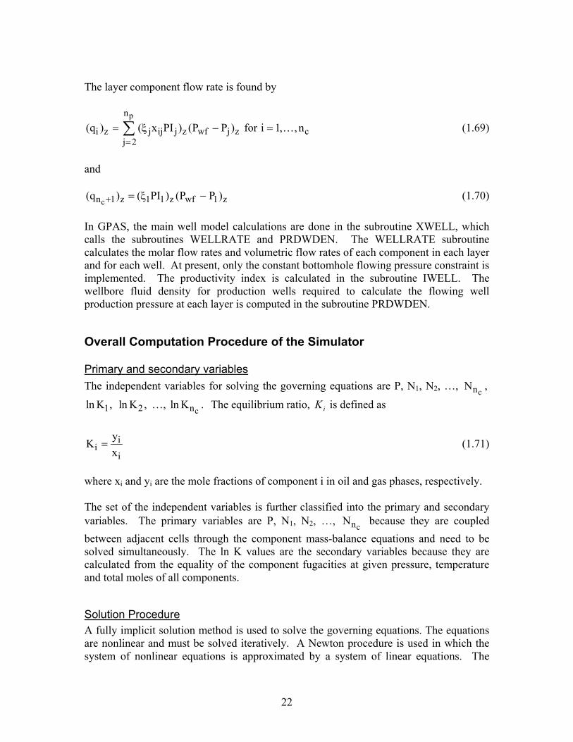
The layer component flow rate is found by
pn
i z j ij j z wf j z cj 2
(q ) ( x PI ) (P P ) for i 1, , n=
= ξ − =∑ … (1.69)
and
cn 1 z 1 1 z wf 1 z(q ) ( PI ) (P P )+ = ξ − (1.70) In GPAS, the main well model calculations are done in the subroutine XWELL, which calls the subroutines WELLRATE and PRDWDEN. The WELLRATE subroutine calculates the molar flow rates and volumetric flow rates of each component in each layer and for each well. At present, only the constant bottomhole flowing pressure constraint is implemented. The productivity index is calculated in the subroutine IWELL. The wellbore fluid density for production wells required to calculate the flowing well production pressure at each layer is computed in the subroutine PRDWDEN.
Overall Computation Procedure of the Simulator
Primary and secondary variables The independent variables for solving the governing equations are P, N1, N2, …, cnN ,
1ln K , 2ln K , …, cnln K . The equilibrium ratio, iK is defined as
ii
i
yK
x= (1.71)
where xi and yi are the mole fractions of component i in oil and gas phases, respectively. The set of the independent variables is further classified into the primary and secondary variables. The primary variables are P, N1, N2, …, cnN because they are coupled between adjacent cells through the component mass-balance equations and need to be solved simultaneously. The ln K values are the secondary variables because they are calculated from the equality of the component fugacities at given pressure, temperature and total moles of all components.
Solution Procedure A fully implicit solution method is used to solve the governing equations. The equations are nonlinear and must be solved iteratively. A Newton procedure is used in which the system of nonlinear equations is approximated by a system of linear equations. The
23
linearization is performed by using the Jacobian Matrix of the governing equations. The Jacobian refers to the matrix whose elements are the derivatives of the governing equations with respect to the independent variables. The sequence of steps involved in the solution of the governing equations for the independent variables over a timestep include:
1. Initialization in Each Gridblock: The Pressure, overall composition and temperature of the fluids in each gridblock are specified. The initialization and calculation of the initial fluid in place is done in the subroutine INFLUID0. This subroutine is the main driver for the computation of the initial fluid in place.
2. Phase identification and Physical Properties Calculation: The flash calculations
are performed in each gridblock and the phase saturations, compositions and densities are determined. The phases are then identified as gas, oil or aqueous phase. Phase viscosities and relative permeabilities are subsequently computed. The flash calculations are performed in the subroutine XFLASH and currently are limited to two phases. The Rachford-Rice equation that determines the phase fractions is coded in the subroutine SOLVE. All the fluid physical properties like the fluid viscosity, relative permeability and phase density calculations are determined in the PROP subroutine. The PROP subroutine calls separate routines to determine the different physical properties. It calls the subroutine LVISC2 to calculate the phase viscosity using the Lorenz coefficient, the subroutine RELPERM3EOS to calculate the three-phase relative permeability using Stone's model or calls the LOOKUP subroutine to interpret the two-phase relative permeability from the relative permeability tables.
3. Governing Equations Linearization: All the governing equations are linearized in
terms of the independent variables and the elements of the Jacobian are calculated. The subroutine JACOBIAN that in turn calls PREROW generates the Jacobian for the linear system. PREROW is the main subroutine that calls the other subroutines, each with a specific task of computing the derivatives of separate equations and terms. The subroutine JACCUM calculates the derivatives of the accumulation term of the component balance. The subroutine JACO2 calculates the derivatives related to transmissibility terms. The subroutine JMASS calculates the derivatives related to the component mass balance in X, Y and Z directions. The derivatives of the source/sink terms are calculated in JSOURCE.
4. Jacobian Factorization and Reduction of the Linear Systems: A row elimination
is performed to reduce the size of the linear system from c2n 1+ to cn for each gridblock. To achieve this, the linearized phase-equilibrium relations and the linearized volume constraint are used to eliminate the secondary variables and one of the overall component moles from the linearized component mass balance equations. The subroutine EOS_JACO forms the Jacobian for row elimination for two-phase cells.
24
5. Solution of the Reduced System of the Linear Equations for the Primary
Variables: The reduced system of linear equations is simultaneously solved for pressure and the overall moles of cn 1− components per unit bulk volume for all the cells.
6. Secondary Variables Calculation: A back substitution method is employed to
compute the secondary variables ln K and overall moles of the component eliminated in Step 4 using the factorized Jacobian. The phase-stability analysis is then carried out for all the gridblocks using the newly updated pressure and overall component moles.
7. Updating Phase Densities and Viscosities, Determination of Single-Phase State
and Estimation of Phase Relative Permeability: The subroutine XUPDATE updates the phase composition and the phase properties as phase density, viscosity, relative permeability and determination of single phase in each cell. The main subroutine in the compositional model EOSCOMP is XSTEP. XSTEP calls XDELTA, which in turn calls the XUPDATE subroutine.
8. Check for Convergence: The residuals of the linear system obtained in Step 3 are
used to determine convergence. If a tolerance is exceeded, the elements of the Jacobian and the residuals of the governing equations are then updated and another Newton iteration is performed by returning to Step 4. If the tolerance is met, a new timestep is then started by returning to Step 3. The subroutine XSTEP is the contact routine between the IPARS framework code and the EOSCOMP compositional model code. The residuals are checked in XSTEP and if the tolerance is met, a new timestep is started, else another Newton iteration is performed.
Executive Routines in EOSCOMP The executive routines in the EOSCOMP model are as follows:
XISDAT All the initial scalar data are read by this subroutine. These include the physical properties of each component, default number of iterations, convergence tolerances for a variety of calculations, output flags, operation specific flags and chemical property data. No grid-element arrays can be reference in this subroutine.
XARRAY This subroutine allocates memory for all the grid element arrays. XIADAT The entire grid element array input as the pressure, water saturation,
feed composition is read in and written out to a file. XIVDAT. Performs the model initialization before time iteration. The PETSc
linear solver is also initialized.
25
XSTEP The main subroutine that performs all the calculations over a
timestep. XQUIT Exits from the simulation when it meets the maximum time,
production limits, or if an error occurs. The communication between processors for the compositional model is performed in the executive subroutines. There is no argument attached to these calls. Those variables associated with grids are passed into these routines through pointers that are stored in common block. These common blocks are included as header files in the subroutines. The executive routines call the work routines to perform all the calculations. The grid dimensions and variables are passed into these work routines through a C routine called CALLWORK, which is handled by the framework. The CALLWORK function passes the variables as an index argument list to the function being called.
Description of the Solver PETSc (Balay et al., 1997; Wang et al., 1999) is a large suite of parallel, general-purpose, object-oriented solvers for the scalable solution of partial differential equations discretized using implicit and semi-implicit methods. PETSc is implemented in C, and is usable from C, Fortran, and C++. It uses MPI for communication across processors. GPAS uses the linear solver component of PETSc to solve the linearized Newton system of equations and uses the parallel data formats provided by PETSc to store the Jacobian and the vectors. The linear solver components of PETSc provides a unified interface to various Krylov methods, such as conjugate gradient (CG), generalized minimal residual (GMRES), biconjugate gradient, etc. and also to various parallel preconditioners such as Jacobi, block preconditioners like block Jacobi, domain decomposition preconditioners like additive Schwartz. GPAS uses the biconjugate gradient stabilized approach as the Krylov method and block Jacobi preconditioner, with point block incomplete factorization (ILU) on the subdomain blocks. The point block refers to treating all the variables associated with a single gridblock as a single unit. The number of subdomain blocks for block Jacobi is chosen to match the number of processors used, so that each processor gets a complete subdomain of the problem and does a single local incomplete factorization on the Jacobian corresponding to this subdomain. For three-phase flow, the compositional model EOSCOMP generates c2n 1+ equations per gridblock causing the Jacobian to have a point-block structure and a point-block sparse storage format is used to store the matrix. These c2n 1+ equations do not result in complete coupling of all the variables across gridblocks. This causes the Jacobian to have some cn 1+ point-block locations with zero values. Thus a block size of cn 1+ is chosen for this matrix type eliminating the need to store the ( )cn 1+ ( )cn 1+ blocks
26
with zero values. The usage of the point-block sparse matrix storage leads to the improvement in the performance of the matrix routines.
Solution Approach in Chemical Module The chemical species were added using two different numerical methods. The species included in the chemical module were any number of conservative and partitioning tracers, electrolytes, polymer, and surfactant. In the first method, we solved the mass balance equations for the aqueous species explicitly. We refer to this formulation as the hybrid method. The chemical module was linked to the equation-of-state compositional model EOSCOMP in an explicit manner. After EOSCOMP solves for the pressures, saturations, and compositions of the non-aqueous species components for a particular time step and the convergence for the mass balance equations is attained, the chemical subroutine imports the required input from the host EOSCOMP and solves for the aqueous species mass balance equation to find the concentration at a given point in space and time. This decoupled approach is more computationally efficient than solving all of the equations simultaneously in EOSCOMP. We, then, formulated and implemented the chemical species in a fully implicit method to take advantage of the larger time steps attainable in the fully implicit formulation. The details of these procedures are given in Task 2.
Non-Orthogonal Grid In the last six months of the project, we have implemented a cornerpoint non-orthogonal grid option to model more realistic reservoir geometries and be able to include the curved reservoir boundaries and impermeable barriers such as shales and faults. The mass balance equation for i-th component assuming diagonal permeability tensor can be written in a Cartesian system as
( ) np npj ji
j ij j xx j ij j yyj 1 j 1
npj
j ij j zz ij 1
Nx K x K
t x x y y
x K q 0z z
= =
=
∂Φ ∂Φ∂ φ ∂ ∂ − ξ λ − ξ λ ∂ ∂ ∂ ∂ ∂
∂Φ∂ − ξ λ − = ∂ ∂
∑ ∑
∑ (1.72)
where Φj is the potential of j phase and is given by
j j jP DΦ = − γ (1.73) In Eq. 1.73 Pj denotes the pressure of j phase and D is depth which is positive in downward direction. Equation 1.72 can be written in a boundary fitted coordinate system using the following transformation
27
(x, y, z) ; (x, y, z) ; (x, y, z)ξ =ξ η = η γ = γ (1.74)
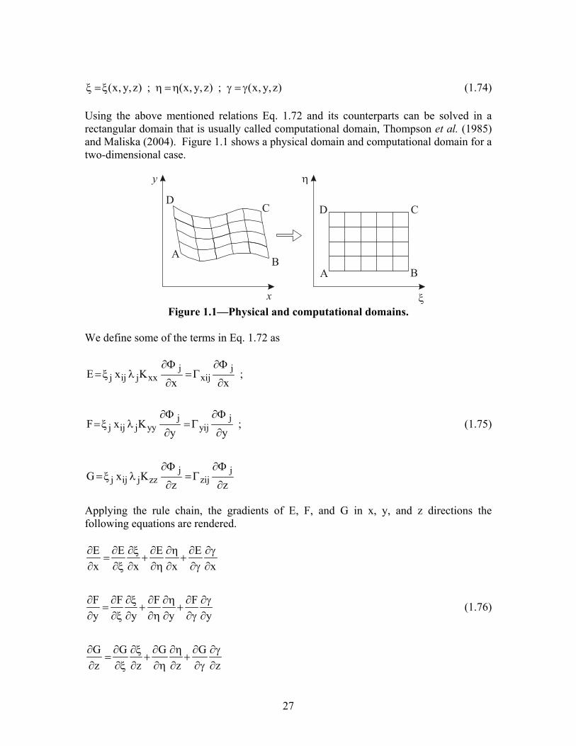
Using the above mentioned relations Eq. 1.72 and its counterparts can be solved in a rectangular domain that is usually called computational domain, Thompson et al. (1985) and Maliska (2004). Figure 1.1 shows a physical domain and computational domain for a two-dimensional case.
x
AB
C
y
A B
C
η
ξ
DD
Figure 1.1—Physical and computational domains.
We define some of the terms in Eq. 1.72 as
j jj ij j xx xij
j jj ij j yy yij
j jj ij j zz zij
E x K ;x x
F x K ;y y
G x Kz z
∂Φ ∂Φ= ξ λ =Γ
∂ ∂
∂Φ ∂Φ=ξ λ =Γ
∂ ∂
∂Φ ∂Φ= ξ λ =Γ
∂ ∂
(1.75)
Applying the rule chain, the gradients of E, F, and G in x, y, and z directions the following equations are rendered.
E E E Ex x x x
F F F Fy y y y
G G G Gz z z z
∂ ∂ ∂ξ ∂ ∂η ∂ ∂γ= + +
∂ ∂ξ ∂ ∂η ∂ ∂γ ∂
∂ ∂ ∂ξ ∂ ∂η ∂ ∂γ= + +
∂ ∂ξ ∂ ∂η ∂ ∂γ ∂
∂ ∂ ∂ξ ∂ ∂η ∂ ∂γ= + +
∂ ∂ξ ∂ ∂η ∂ ∂γ ∂
(1.76)
28
Dividing each term of Eq. 1.76 by Jt, the Jacobian of the transformation, and replacing the result in Eq. 1.72, and adding and subtracting terms of type
yx z
t t tE 'F ,G
J J Jξ ξ ξ∂ ∂ ∂
∂ξ ∂ξ ∂ξ and after simplifications, the following conservative
equation is obtained:
x y z x y z x y zi
t t t t
y y yx x x
t t t t t t
E F G E F G E F GNt J J J J
E FJ J J J J J
G
ξ + ξ + ξ η + η + η γ + γ + γ φ∂ ∂ ∂ ∂− − − ∂ ∂ξ ∂η ∂γ
ξ η γ ξ η γ∂ ∂ ∂ ∂ ∂ ∂− + + − + + ∂ξ ∂η ∂γ ∂ξ ∂η ∂γ
∂− z z z i
t t t t
q0
J J J J ξ η γ∂ ∂
+ + − = ∂ξ ∂η ∂γ
(1.77)
It is easy to demonstrate that the terms in blankets in Eq. 1.77 are equal to zero. Details can be found in Maliska (2004). Applying the chain rule to E, F, and G and inserting the results into Eq. 1.77, we obtain
( ) ( )
( )
np npj j2 2 2i
x xij y yij z zij x x xij y y yij z z zijt t tj 1 j 1
np npj
x x xij y y yij z z zij x x xij y y yij zt tj 1 j 1
N 1 1t J J J
1 1J J
= =
= =
∂Φ ∂Φ ∂ φ ∂ ∂ − ξ Γ +ξ Γ +ξ Γ − ξ η Γ +ξ η Γ + ξ η Γ ∂ ∂ξ ∂ξ ∂ξ ∂η ∂Φ∂ ∂ − ξ γ Γ +ξ γ Γ + ξ γ Γ − ξ η Γ + ξ η Γ + ξ
∂ξ ∂γ ∂η
∑ ∑
∑ ∑ ( )
( ) ( )
( )
jz zij
np npj j2 2 2
x xij y yij z zij x x xij y y yij z z zijt tj 1 j 1
np npj
x x xij y y yij z z zij x x xij y y yt tj 1 j 1
1 1J J
1 1J J
= =
= =
∂Φ η Γ
∂ξ ∂Φ ∂Φ∂ ∂ − η Γ + η Γ +η Γ − η γ Γ + η γ Γ + η γ Γ
∂η ∂η ∂η ∂γ ∂Φ∂ ∂ − ξ γ Γ + ξ γ Γ + ξ γ Γ − η γ Γ + η γ Γ
∂γ ∂ξ ∂γ
∑ ∑
∑ ∑ ( )
( )
jij z z zij
npj2 2 2 i
x xij y yij z zijt tj 1
1 q 0J J=
∂Φ + η γ Γ
∂γ ∂Φ∂ − γ Γ + γ Γ + γ Γ − =
∂γ ∂γ ∑
(1.78)
where the direct metrics and the Jacobian (Jt) of the transformation can be evaluated as a function of the inverse metrics by
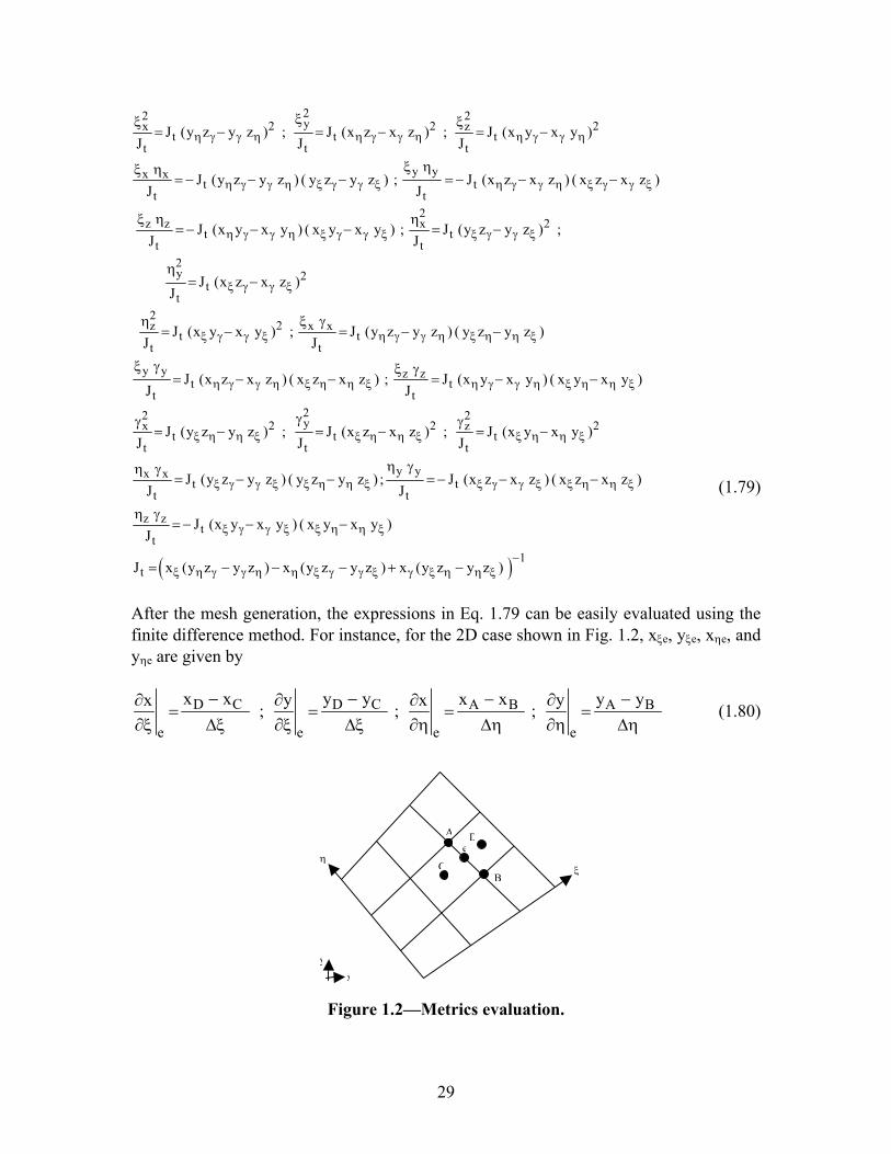
29
22 2y2 2 2x zt t t
t t t
y yx xt t
t t2
2z z xt t
t t2y
tt
J (y z y z ) ; J (x z x z ) ; J (x y x y )J J J
J (y z y z ) ( y z y z ) ; J (x z x z ) ( x z x z )J J
J (x y x y ) ( x y x y ) ; J (y z y z ) ;J J
J (x z x z )J
η γ γ η η γ γ η η γ γ η
η γ γ η ξ γ γ ξ η γ γ η ξ γ γ ξ
η γ γ η ξ γ γ ξ ξ γ γ ξ
ξ γ γ ξ
ξξ ξ= − = − = −
ξ ηξ η= − − − = − − −
ξ η η= − − − = −
η= − 2
22z x x
t tt t
y y z zt t
t t22 2y2 2 2x z
t t tt t t
x xt
t
J (x y x y ) ; J (y z y z ) ( y z y z )J J
J (x z x z ) ( x z x z ) ; J (x y x y ) ( x y x y )J J
J (y z y z ) ; J (x z x z ) ; J (x y x y )J J J
J (y z y z ) ( yJ
ξ γ γ ξ η γ γ η ξ η η ξ
η γ γ η ξ η η ξ η γ γ η ξ η η ξ
ξ η η ξ ξ η η ξ ξ η η ξ
ξ γ γ ξ
η ξ γ= − = − −
ξ γ ξ γ= − − = − −
γγ γ= − = − = −
η γ= −
( )
y yt
t
z zt
t1
t
z y z ) ; J (x z x z ) ( x z x z )J
J (x y x y ) ( x y x y )J
J x (y z y z ) x (y z y z ) x (y z y z )
ξ η η ξ ξ γ γ ξ ξ η η ξ
ξ γ γ ξ ξ η η ξ
−ξ η γ γ η η ξ γ γ ξ γ ξ η η ξ
η γ− = − − −
η γ= − − −
= − − − + −
(1.79)
After the mesh generation, the expressions in Eq. 1.79 can be easily evaluated using the finite difference method. For instance, for the 2D case shown in Fig. 1.2, xξe, yξe, xηe, and yηe are given by
D C D C A B A B
e e e e
x x y y x x y yy yx x; ; ;− − − −∂ ∂∂ ∂
= = = =∂ξ ∆ξ ∂ξ ∆ξ ∂η ∆η ∂η ∆η
(1.80)
xy
e
B
A
C
D
η ξ
Figure 1.2—Metrics evaluation.
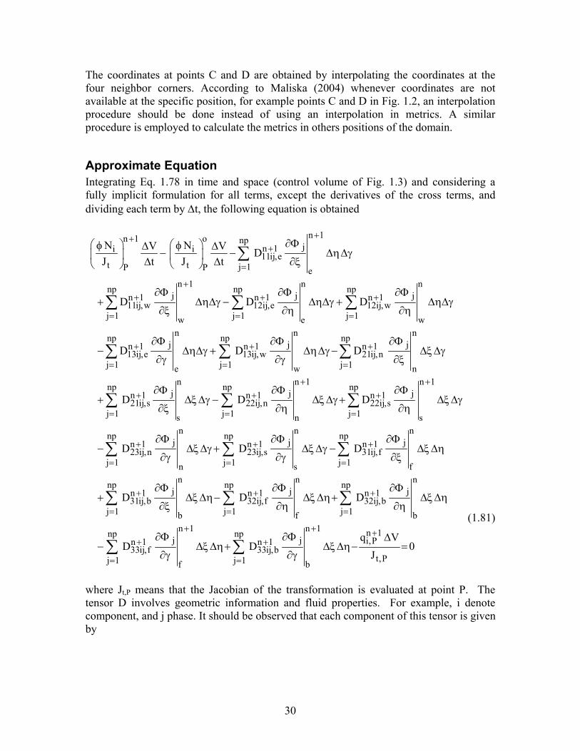
30
The coordinates at points C and D are obtained by interpolating the coordinates at the four neighbor corners. According to Maliska (2004) whenever coordinates are not available at the specific position, for example points C and D in Fig. 1.2, an interpolation procedure should be done instead of using an interpolation in metrics. A similar procedure is employed to calculate the metrics in others positions of the domain.
Approximate Equation Integrating Eq. 1.78 in time and space (control volume of Fig. 1.3) and considering a fully implicit formulation for all terms, except the derivatives of the cross terms, and dividing each term by ∆t, the following equation is obtained
n 1n 1 o npjn 1i i
11ij,et t j 1P P e
n 1 n nnp np npj j jn 1 n 1 n 1
11ij,w 12ij,e 12ij,wj 1 j 1 j 1w e w
nnp npjn 1 n 1
13ij,e 13ij,wj 1 j 1e
N NV V DJ t J t
D D D
D D
+++
=
++ + +
= = =
+ +
= =
∂Φ φ φ∆ ∆− − ∆η∆γ ∆ ∆ ∂ξ
∂Φ ∂Φ ∂Φ+ ∆η∆γ − ∆η∆γ + ∆η∆γ
∂ξ ∂η ∂η
∂Φ ∂Φ− ∆η∆γ +
∂γ
∑
∑ ∑ ∑
∑ ∑n nnp
j jn 121ij,n
j 1w nn n 1 n 1np np np
j j jn 1 n 1 n 121ij,s 22ij,n 22ij,s
j 1 j 1 j 1s n sn nnp np np
j jn 1 n 1 n 123ij,n 23ij,s 31ij,f
j 1 j 1 j 1n s
D
D D D
D D D
+
=
+ ++ + +
= = =
+ + +
= = =
∂Φ∆η∆γ − ∆ξ ∆γ
∂γ ∂ξ
∂Φ ∂Φ ∂Φ+ ∆ξ ∆γ − ∆ξ ∆γ + ∆ξ ∆γ
∂ξ ∂η ∂η
∂Φ ∂Φ ∂Φ− ∆ξ ∆γ + ∆ξ ∆γ −
∂γ ∂γ
∑
∑ ∑ ∑
∑ ∑ ∑n
j
fn n nnp np np
j j jn 1 n 1 n 131ij,b 32ij,f 32ij,b
j 1 j 1 j 1b f bn 1 n 1 n 1np np
j j i,Pn 1 n 133ij,f 33ij,b
t,Pj 1 j 1f b
D D D
q VD D 0
J
+ + +
= = =
+ + ++ +
= =
∆ξ ∆η∂ξ
∂Φ ∂Φ ∂Φ+ ∆ξ ∆η− ∆ξ ∆η+ ∆ξ ∆η
∂ξ ∂η ∂η
∂Φ ∂Φ ∆− ∆ξ ∆η+ ∆ξ ∆η− =
∂γ ∂γ
∑ ∑ ∑
∑ ∑
(1.81)
where Jt,P means that the Jacobian of the transformation is evaluated at point P. The tensor D involves geometric information and fluid properties. For example, i denote component, and j phase. It should be observed that each component of this tensor is given by
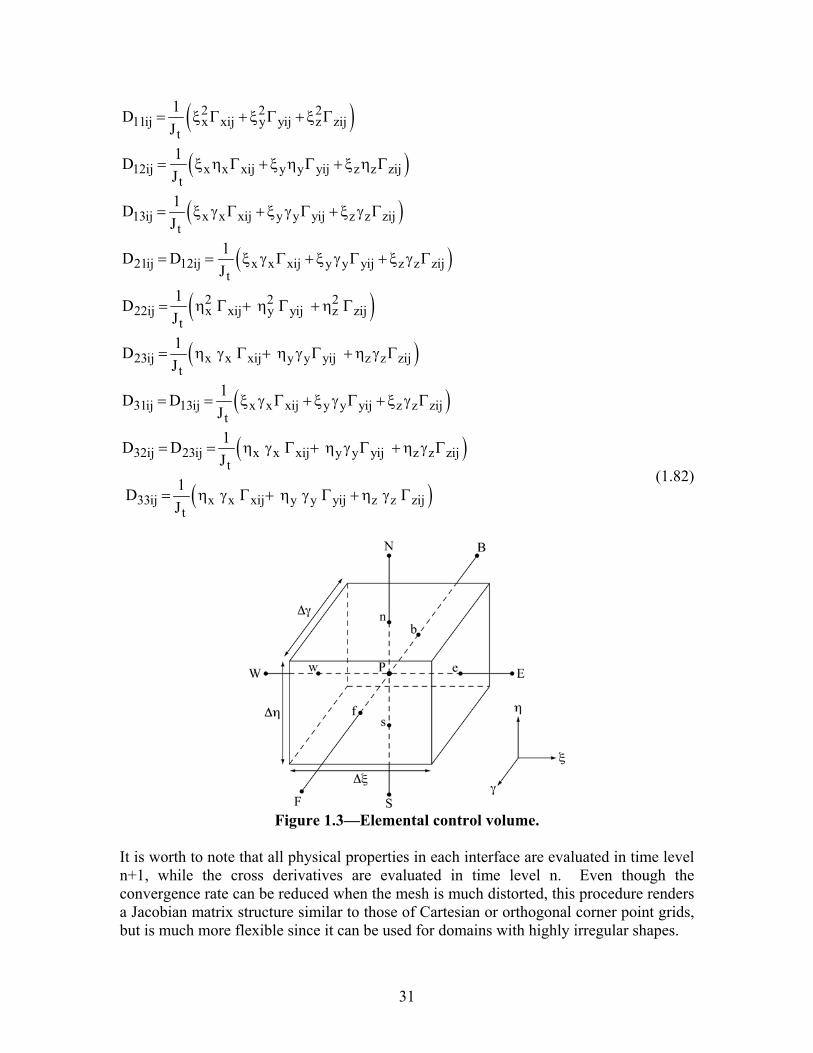
31
( )( )
( )
( )
( )
2 2 211ij x xij y yij z zij
t
12ij x x xij y y yij z z zijt
13ij x x xij y y yij z z zijt
21ij 12ij x x xij y y yij z z zijt
2 2 222ij x xij y yij z zij
t
23ij x x xij y y yit
1DJ1DJ1DJ
1D DJ
1DJ1DJ
= ξ Γ + ξ Γ + ξ Γ
= ξ η Γ + ξ η Γ + ξ η Γ
= ξ γ Γ + ξ γ Γ + ξ γ Γ
= = ξ γ Γ + ξ γ Γ + ξ γ Γ
= η Γ + η Γ + η Γ
= η γ Γ + η γ Γ( )
( )
( )
( )
j z z zij
31ij 13ij x x xij y y yij z z zijt
32ij 23ij x x xij y y yij z z zijt
33ij x x xij y y yij z z zijt
1D DJ1D DJ
1DJ
+ η γ Γ
= = ξ γ Γ + ξ γ Γ + ξ γ Γ
= = η γ Γ + η γ Γ + η γ Γ
= η γ Γ + η γ Γ + η γ Γ (1.82)
Figure 1.3—Elemental control volume.
It is worth to note that all physical properties in each interface are evaluated in time level n+1, while the cross derivatives are evaluated in time level n. Even though the convergence rate can be reduced when the mesh is much distorted, this procedure renders a Jacobian matrix structure similar to those of Cartesian or orthogonal corner point grids, but is much more flexible since it can be used for domains with highly irregular shapes.
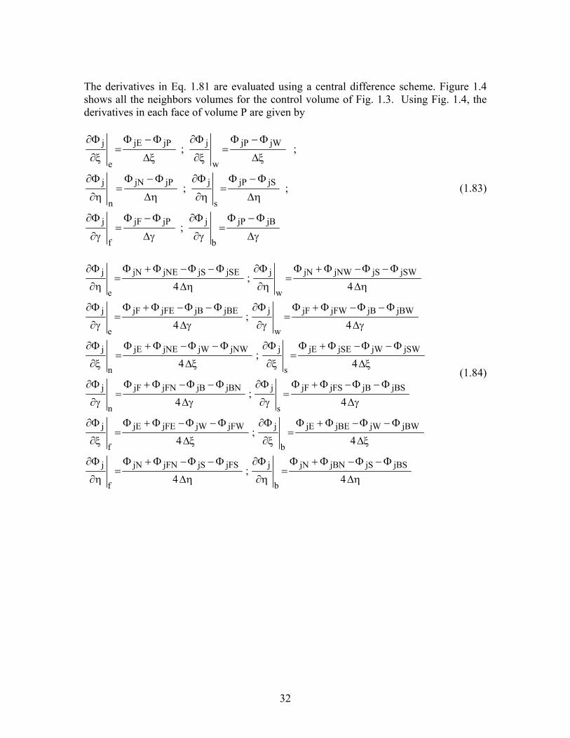
32
The derivatives in Eq. 1.81 are evaluated using a central difference scheme. Figure 1.4 shows all the neighbors volumes for the control volume of Fig. 1.3. Using Fig. 1.4, the derivatives in each face of volume P are given by
j jE jP j jP jW
e w
j jN jP j jP jS
n s
j jF jP j jP jB
f b
; ;
; ;
;
∂Φ Φ − Φ ∂Φ Φ − Φ= =
∂ξ ∆ξ ∂ξ ∆ξ
∂Φ Φ − Φ ∂Φ Φ − Φ= =
∂η ∆η ∂η ∆η
∂Φ Φ − Φ ∂Φ Φ − Φ= =
∂γ ∆γ ∂γ ∆γ
(1.83)
j jN jNE jS jSE j jN jNW jS jSW
e w
j jF jFE jB jBE j jF jFW jB jBW
e w
j jE jNE jW jNW j jE jSE jW jSW
n s
j jF jFN jB jBN j
n s
;4 4
;4 4
;4 4
;4
∂Φ Φ + Φ −Φ − Φ ∂Φ Φ + Φ −Φ − Φ= =
∂η ∆η ∂η ∆η
∂Φ Φ + Φ −Φ − Φ ∂Φ Φ + Φ −Φ − Φ= =
∂γ ∆γ ∂γ ∆γ
∂Φ Φ + Φ −Φ − Φ ∂Φ Φ + Φ −Φ − Φ= =
∂ξ ∆ξ ∂ξ ∆ξ
∂Φ Φ + Φ −Φ − Φ ∂Φ= =
∂γ ∆γ ∂γjF jFS jB jBS
j jE jFE jW jFW j jE jBE jW jBW
f b
j jN jFN jS jFS j jN jBN jS jBS
f b
4
;4 4
;4 4
Φ + Φ −Φ − Φ
∆γ
∂Φ Φ + Φ −Φ − Φ ∂Φ Φ + Φ −Φ − Φ= =
∂ξ ∆ξ ∂ξ ∆ξ
∂Φ Φ + Φ −Φ − Φ ∂Φ Φ + Φ −Φ − Φ= =
∂η ∆η ∂η ∆η
(1.84)
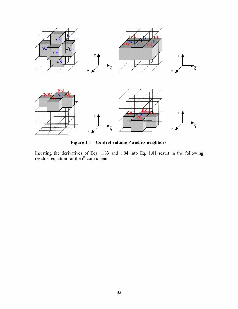
33
• P • W • F
• E
• N
• S
B
ξ
η
γ
• P• E
• N W E F
B P FE
BE BWFW
ξ
η
γ
NEBN
NW FN
N
ξ
η
γ
SE BS SWFS
S
ξ
η
γ
Figure 1.4—Control volume P and its neighbors.
Inserting the derivatives of Eqs. 1.83 and 1.84 into Eq. 1.81 result in the following residual equation for the ith component
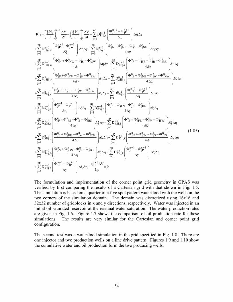
34
n 1 n 1n 1 o npjE jPn 1i i
iP 11ij,eP P j 1
n 1 n 1 n n n nnp npjP jW jN jNE jS jSEn 1 n 1
11ij,w 12ij,ej 1 j 1
npjNn 1
12ij,wj 1
N NV VR DJ t J t
D D4
D
+ +++
=
+ ++ +
= =
+
=
Φ − Φφ φ∆ ∆ = − − ∆η∆γ ∆ ∆ ∆ξ Φ − Φ Φ + Φ −Φ − Φ + ∆η∆γ − ∆η∆γ ∆ξ ∆η
Φ+
∑
∑ ∑
∑n n n n n n n nnp
jNW jS jSW jF jFE jB jBEn 113ij,e
j 1
n n n n n n n nnp npjF jFW jB jBW jE jNE jW jNWn 1 n 1
13ij,w 21ij,nj 1 j 1
21ij,s
D4 4
D D4 4
D
+
=
+ +
= =
+ Φ −Φ − Φ Φ + Φ −Φ − Φ ∆η∆γ − ∆η∆γ ∆η ∆γ Φ + Φ −Φ − Φ Φ + Φ −Φ − Φ + ∆η∆γ − ∆ξ ∆γ ∆γ ∆ξ
+
∑
∑ ∑
n n n n n 1 n 1np npjE jSE jW jSW jN jPn 1 n 1
22ij,nj 1 j 1
n 1 n 1 n n n nnp npjP jS jF jFN jB jBNn 1 n 1
22ij,s 23ij,nj 1 j 1
n 123ij,s
j 1
D4
D D4
D
+ ++ +
= =
+ ++ +
= =
+
=
Φ + Φ −Φ − Φ Φ − Φ ∆ξ ∆γ − ∆ξ ∆γ ∆ξ ∆η Φ − Φ Φ + Φ −Φ − Φ + ∆ξ∆γ − ∆ξ ∆γ ∆η ∆γ
+
∑ ∑
∑ ∑
n n n n n n n nnp npjF jFS jB jBS jE jFE jW jFWn 1
31ij,fj 1
n n n n n n n nnp npjE jBE jW jBW jN jFN jS jFSn 1 n 1
31ij,b 32ij,fj 1 j 1
D4 4
D D4 4
D
+
=
+ +
= =
Φ + Φ −Φ − Φ Φ + Φ −Φ − Φ ∆ξ ∆γ − ∆ξ ∆η ∆γ ∆ξ Φ + Φ −Φ − Φ Φ + Φ −Φ − Φ + ∆ξ ∆η − ∆ξ ∆η ∆ξ ∆η
+
∑ ∑
∑ ∑
n n n n n 1 n 1np npjN jBN jS jBS jF jPn 1 n 1
32ij,b 33ij,fj 1 j 1
n 1 n 1 n 1npjF jP i,Pn 1
33ij,btPj 1
D4
q VD 0
J
+ ++ +
= =
+ + ++
=
Φ + Φ −Φ − Φ Φ − Φ ∆ξ ∆η − ∆ξ ∆η ∆η ∆γ Φ − Φ ∆ + ∆ξ ∆η− = ∆γ
∑ ∑
∑
(1.85)
The formulation and implementation of the corner point grid geometry in GPAS was verified by first comparing the results of a Cartesian grid with that shown in Fig. 1.5. The simulation is based on a quarter of a five spot pattern waterflood with the wells in the two corners of the simulation domain. The domain was discretized using 16x16 and 32x32 number of gridblocks in x and y directions, respectively. Water was injected in an initial oil saturated reservoir at the residual water saturation. The water production rates are given in Fig. 1.6. Figure 1.7 shows the comparison of oil production rate for these simulations. The results are very similar for the Cartesian and corner point grid configuration. The second test was a waterflood simulation in the grid specified in Fig. 1.8. There are one injector and two production wells on a line drive pattern. Figures 1.9 and 1.10 show the cumulative water and oil production form the two producing wells.
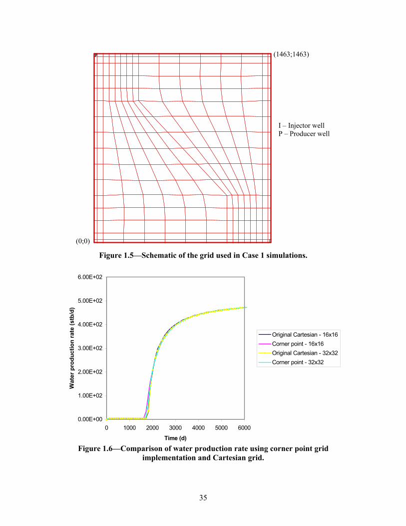
35
I
P
I – Injector well P – Producer well
(0;0)
(1463;1463)
Figure 1.5—Schematic of the grid used in Case 1 simulations.
0.00E+00
1.00E+02
2.00E+02
3.00E+02
4.00E+02
5.00E+02
6.00E+02
0 1000 2000 3000 4000 5000 6000
Time (d)
Wat
er p
rodu
ctio
n ra
te (s
tb/d
)
Original Cartesian - 16x16Corner point - 16x16Original Cartesian - 32x32Corner point - 32x32
Figure 1.6—Comparison of water production rate using corner point grid
implementation and Cartesian grid.
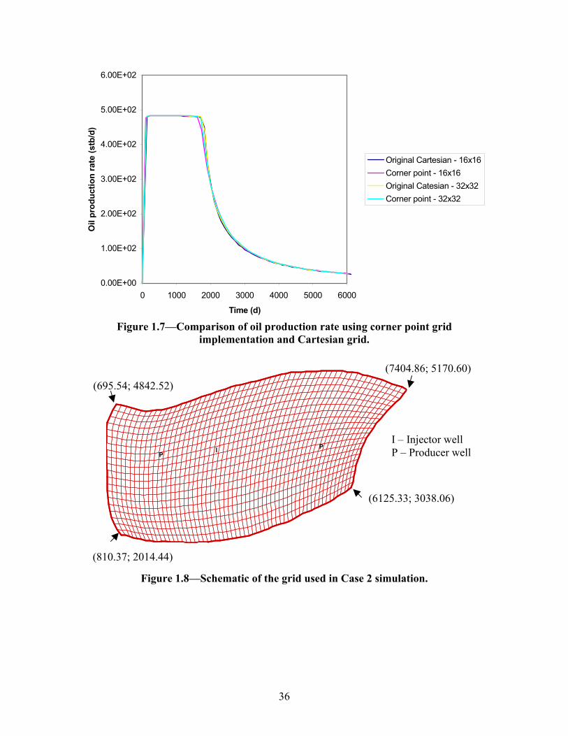
36
0.00E+00
1.00E+02
2.00E+02
3.00E+02
4.00E+02
5.00E+02
6.00E+02
0 1000 2000 3000 4000 5000 6000
Time (d)
Oil
prod
uctio
n ra
te (s
tb/d
)
Original Cartesian - 16x16Corner point - 16x16Original Catesian - 32x32Corner point - 32x32
Figure 1.7—Comparison of oil production rate using corner point grid
implementation and Cartesian grid.
I PP
(810.37; 2014.44)
(7404.86; 5170.60)
I – Injector well P – Producer well
(6125.33; 3038.06)
(695.54; 4842.52)
Figure 1.8—Schematic of the grid used in Case 2 simulation.
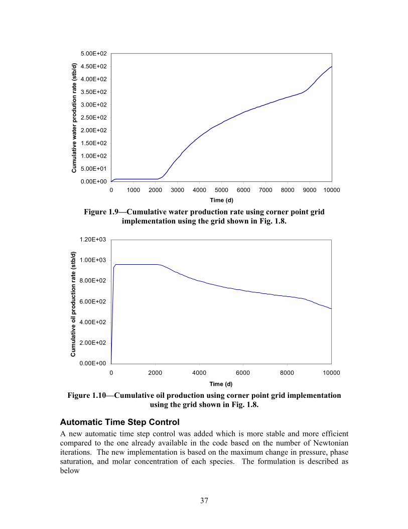
37
0.00E+00
5.00E+01
1.00E+02
1.50E+02
2.00E+02
2.50E+02
3.00E+02
3.50E+02
4.00E+02
4.50E+02
5.00E+02
0 1000 2000 3000 4000 5000 6000 7000 8000 9000 10000
Time (d)
Cum
ulat
ive
wat
er p
rodu
tion
rate
(stb
/d)
Figure 1.9—Cumulative water production rate using corner point grid
implementation using the grid shown in Fig. 1.8.
0.00E+00
2.00E+02
4.00E+02
6.00E+02
8.00E+02
1.00E+03
1.20E+03
0 2000 4000 6000 8000 10000
Time (d)
Cum
ulat
ive
oil p
rodu
ctio
n ra
te (s
tb/d
)
Figure 1.10—Cumulative oil production using corner point grid implementation
using the grid shown in Fig. 1.8.
Automatic Time Step Control A new automatic time step control was added which is more stable and more efficient compared to the one already available in the code based on the number of Newtonian iterations. The new implementation is based on the maximum change in pressure, phase saturation, and molar concentration of each species. The formulation is described as below
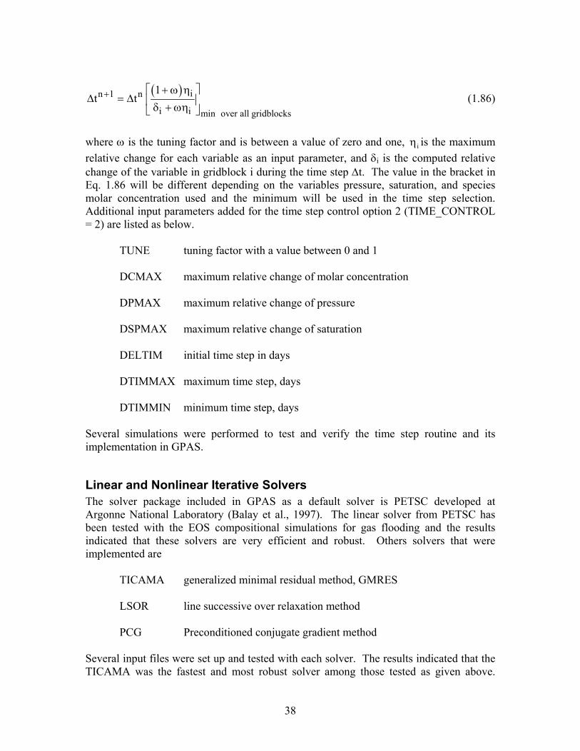
38
( ) in 1 n
i i min over all gridblocks
1t t+ + ω η
∆ = ∆ δ + ωη (1.86)
where ω is the tuning factor and is between a value of zero and one, iη is the maximum relative change for each variable as an input parameter, and δi is the computed relative change of the variable in gridblock i during the time step ∆t. The value in the bracket in Eq. 1.86 will be different depending on the variables pressure, saturation, and species molar concentration used and the minimum will be used in the time step selection. Additional input parameters added for the time step control option 2 (TIME_CONTROL = 2) are listed as below.
TUNE tuning factor with a value between 0 and 1 DCMAX maximum relative change of molar concentration DPMAX maximum relative change of pressure DSPMAX maximum relative change of saturation DELTIM initial time step in days DTIMMAX maximum time step, days DTIMMIN minimum time step, days
Several simulations were performed to test and verify the time step routine and its implementation in GPAS.
Linear and Nonlinear Iterative Solvers The solver package included in GPAS as a default solver is PETSC developed at Argonne National Laboratory (Balay et al., 1997). The linear solver from PETSC has been tested with the EOS compositional simulations for gas flooding and the results indicated that these solvers are very efficient and robust. Others solvers that were implemented are
TICAMA generalized minimal residual method, GMRES LSOR line successive over relaxation method PCG Preconditioned conjugate gradient method
Several input files were set up and tested with each solver. The results indicated that the TICAMA was the fastest and most robust solver among those tested as given above.
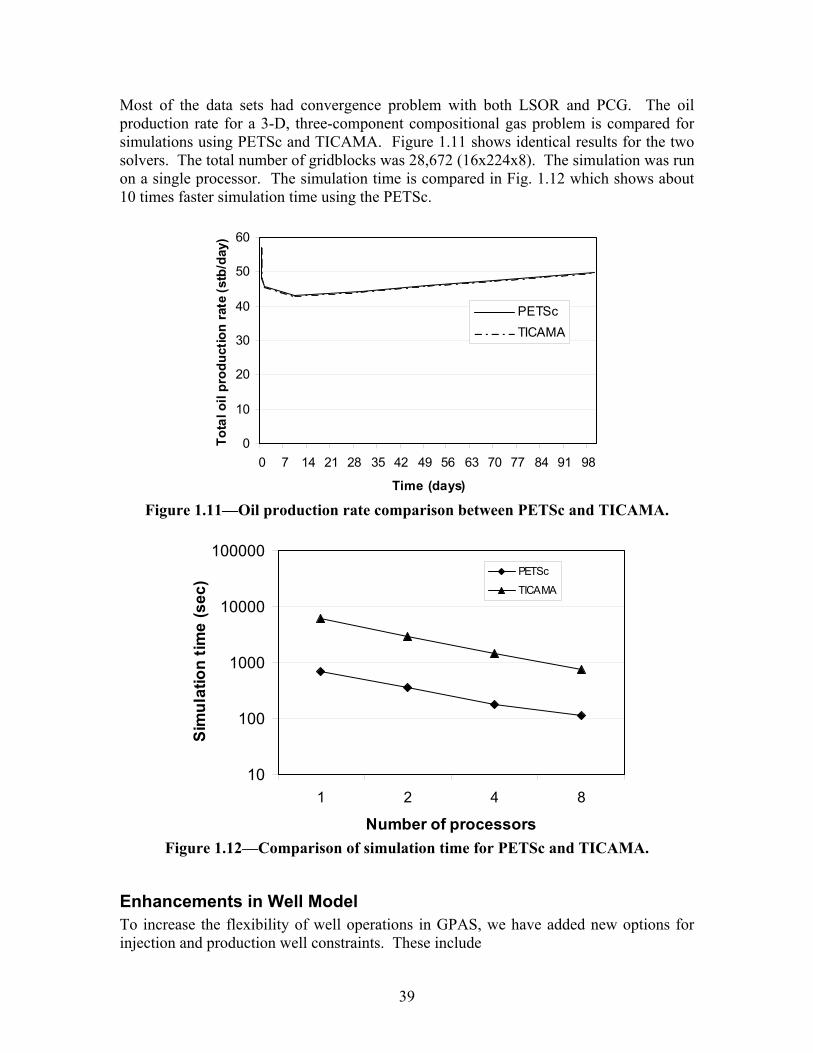
39
Most of the data sets had convergence problem with both LSOR and PCG. The oil production rate for a 3-D, three-component compositional gas problem is compared for simulations using PETSc and TICAMA. Figure 1.11 shows identical results for the two solvers. The total number of gridblocks was 28,672 (16x224x8). The simulation was run on a single processor. The simulation time is compared in Fig. 1.12 which shows about 10 times faster simulation time using the PETSc.
0
10
20
30
40
50
60
0 7 14 21 28 35 42 49 56 63 70 77 84 91 98
Time (days)
Tota
l oil
prod
uctio
n ra
te (s
tb/d
ay)
PETScTICAMA
Figure 1.11—Oil production rate comparison between PETSc and TICAMA.
10
100
1000
10000
100000
1 2 4 8
Number of processors
Sim
ulat
ion
time
(sec
)
PETSc
TICAMA
Figure 1.12—Comparison of simulation time for PETSc and TICAMA.
Enhancements in Well Model To increase the flexibility of well operations in GPAS, we have added new options for injection and production well constraints. These include
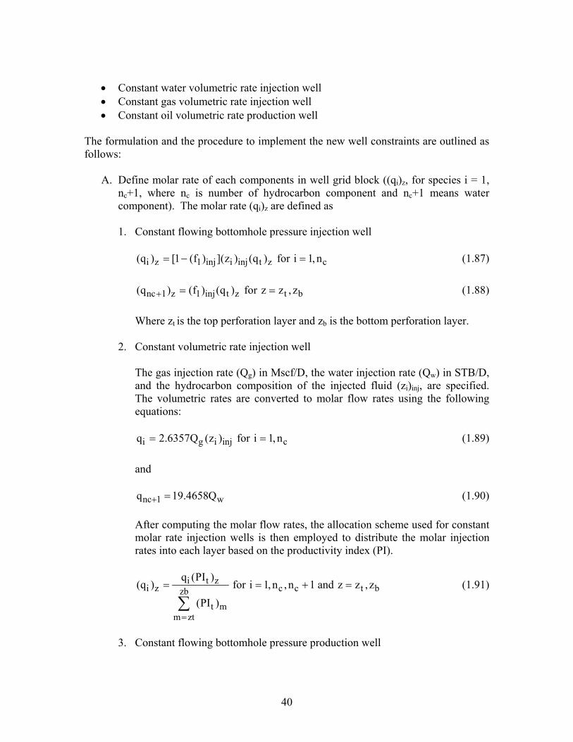
40
• Constant water volumetric rate injection well • Constant gas volumetric rate injection well • Constant oil volumetric rate production well
The formulation and the procedure to implement the new well constraints are outlined as follows:
A. Define molar rate of each components in well grid block ((qi)z, for species i = 1, nc+1, where nc is number of hydrocarbon component and nc+1 means water component). The molar rate (qi)z are defined as
1. Constant flowing bottomhole pressure injection well i z 1 inj i inj t z c(q ) [1 (f ) ](z ) (q ) for i 1, n= − = (1.87) nc 1 z 1 inj t z t b(q ) (f ) (q ) for z z , z+ = = (1.88) Where zt is the top perforation layer and zb is the bottom perforation layer. 2. Constant volumetric rate injection well The gas injection rate (Qg) in Mscf/D, the water injection rate (Qw) in STB/D,
and the hydrocarbon composition of the injected fluid (zi)inj, are specified. The volumetric rates are converted to molar flow rates using the following equations:
i g i inj cq 2.6357Q (z ) for i 1, n= = (1.89) and nc 1 wq 19.4658Q+ = (1.90) After computing the molar flow rates, the allocation scheme used for constant
molar rate injection wells is then employed to distribute the molar injection rates into each layer based on the productivity index (PI).
i t zi z c c t bzb
t mm zt
q (PI )(q ) for i 1, n , n 1 and z z , z
(PI )=
= = + =
∑ (1.91)
3. Constant flowing bottomhole pressure production well
41
np
i z j ij j z wf j z c t bj 2
(q ) ( x PI ) (P P ) for i 1, n and z z to z=
= ξ − = =∑ (1.92)
and nc 1 z 1 1 z wf 1 z t b(q ) ( PI ) (P P ) for z z to z+ = ξ − = (1.93) 4. Constant oil volumetric rate production well The oil rate production in STB/D, Qo is specified in this option. A flash
calculation is done at separator conditions to determine the molar fraction of oil phase, (Lo)prod, in the produced hydrocarbon fluid using the overall hydrocarbon composition computed by
npzbj ij j m
m zt j 2i prod cnpzb
j j mm zt j 2
( x PI )
(z ) for i 1, n
( PI )
= =
= =
ξ
= =
ξ
∑ ∑
∑ ∑ (1.94)
The total molar flow rate is then calculated using
npzbj j m
m zt j 1ot npzbo prod o prod
j j mm zt j 2
( PI )5.6146Q
q(L ) (v )
( PI )
= =
= =
ξ
=
ξ
∑ ∑
∑ ∑ (1.95)
where (vo)prod is the molar volume of the oil phase at the separator conditions.
The same allocation scheme for constant molar rate production wells is used to compute the layer component rates.
When the total molar production rate (qt) is specified, the total production rate
for each layer is calculated using:
np
t j j zj 1
t z t bnpzbj j m
m zt j 1
q ( PI )
(q ) for z z , z
( PI )
=
= =
ξ
= =
ξ
∑
∑ ∑ (1.96)
The layer component rates are found by
42
np
t z j ij j zj 2
i z c t bnp
j j zj 1
(q ) ( x PI )
(q ) for i 1, n and z z to z
( PI )
=
=
ξ
= = =
ξ
∑
∑ (1.97)
and
t z 1 1 znc 1 z t bnp
j j zj 1
(q ) ( PI )(q ) for z z to z
( PI )+
=
ξ= =
ξ∑ (1.98)
The (qi)z are added to residuals of species conservation equations for each
components. ARM(i) = ARM(i) + (qi)z for i = 1, nc (1.99) ARW = ARW + (qnc+1)z (1.100)
B. Derive the derivatives of (qi)z w.r.t. independent variables (ln K1, …, ln Knc, N1, …, Nnc, P, Nw).
C. Modify the elements of the Jacobian matrix. The derivatives in Step B are
subtracted from the existing Jacobian for the species mass conservation equations. For hydrocarbon components:
i zc
j
(q )AMK(i, j) AMK(i, j) for i, j 1, , nln K
∂= − =
∂… (1.101)
i zc
j
(q )AMNP(i, j) AMNP(i, j) for i, j 1, , nN
∂= − =
∂… (1.102)
i z(q )AMNP(i, j 1) AMNP(i, j 1)P
∂+ = + −
∂ (1.103)
i z
w
(q )AMW(i) AMW(i)N
∂= −
∂ (1.104)
For water components:
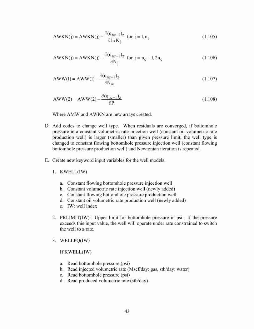
43
nc 1 zc
j
(q )AWKN(j) AWKN(j) for j 1, n
ln K+∂
= − =∂
(1.105)
nc 1 zc c
j
(q )AWKN(j) AWKN(j) for j n 1, 2n
N+∂
= − = +∂
(1.106)
nc 1 z
w
(q )AWW(1) AWW(1)N
+∂= −
∂ (1.107)
nc 1 z(q )AWW(2) AWW(2)P+∂
= −∂
(1.108)
Where AMW and AWKN are new arrays created. D. Add codes to change well type. When residuals are converged, if bottomhole
pressure in a constant volumetric rate injection well (constant oil volumetric rate production well) is larger (smaller) than given pressure limit, the well type is changed to constant flowing bottomhole pressure injection well (constant flowing bottomhole pressure production well) and Newtonian iteration is repeated.
E. Create new keyword input variables for the well models.
1. KWELL(IW)
a. Constant flowing bottomhole pressure injection well b. Constant volumetric rate injection well (newly added) c. Constant flowing bottomhole pressure production well d. Constant oil volumetric rate production well (newly added) e. IW: well index
2. PRLIMIT(IW): Upper limit for bottomhole pressure in psi. If the pressure
exceeds this input value, the well will operate under rate constrained to switch the well to a rate.
3. WELLPQ(IW) If KWELL(IW)
a. Read bottomhole pressure (psi) b. Read injected volumetric rate (Mscf/day: gas, stb/day: water) c. Read bottomhole pressure (psi) d. Read produced volumetric rate (stb/day)
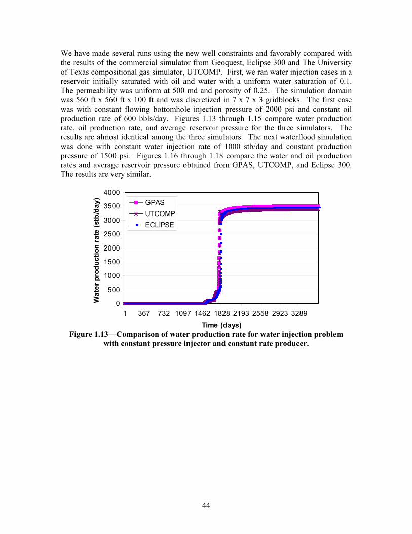
44
We have made several runs using the new well constraints and favorably compared with the results of the commercial simulator from Geoquest, Eclipse 300 and The University of Texas compositional gas simulator, UTCOMP. First, we ran water injection cases in a reservoir initially saturated with oil and water with a uniform water saturation of 0.1. The permeability was uniform at 500 md and porosity of 0.25. The simulation domain was 560 ft x 560 ft x 100 ft and was discretized in 7 x 7 x 3 gridblocks. The first case was with constant flowing bottomhole injection pressure of 2000 psi and constant oil production rate of 600 bbls/day. Figures 1.13 through 1.15 compare water production rate, oil production rate, and average reservoir pressure for the three simulators. The results are almost identical among the three simulators. The next waterflood simulation was done with constant water injection rate of 1000 stb/day and constant production pressure of 1500 psi. Figures 1.16 through 1.18 compare the water and oil production rates and average reservoir pressure obtained from GPAS, UTCOMP, and Eclipse 300. The results are very similar.
0
500
1000
1500
2000
2500
3000
3500
4000
1 367 732 1097 1462 1828 2193 2558 2923 3289Time (days)
Wat
er p
rodu
ctio
n ra
te (s
tb/d
ay)
GPASUTCOMPECLIPSE
Figure 1.13—Comparison of water production rate for water injection problem
with constant pressure injector and constant rate producer.
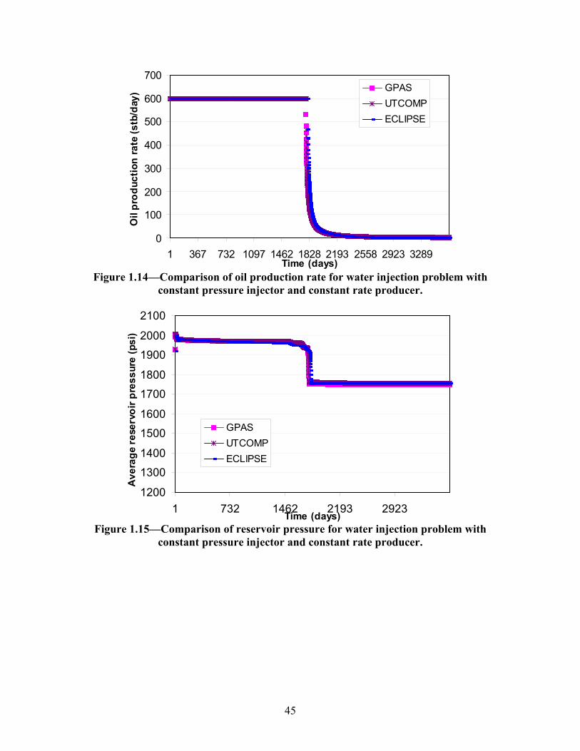
45
0
100
200
300
400
500
600
700
1 367 732 1097 1462 1828 2193 2558 2923 3289Time (days)
Oil
prod
uctio
n ra
te (s
tb/d
ay) GPAS
UTCOMPECLIPSE
Figure 1.14—Comparison of oil production rate for water injection problem with
constant pressure injector and constant rate producer.
1200
1300
1400
1500
1600
1700
1800
1900
2000
2100
1 732 1462 2193 2923Time (days)
Ave
rage
res
ervo
ir pr
essu
re (p
si)
GPASUTCOMPECLIPSE
Figure 1.15—Comparison of reservoir pressure for water injection problem with
constant pressure injector and constant rate producer.
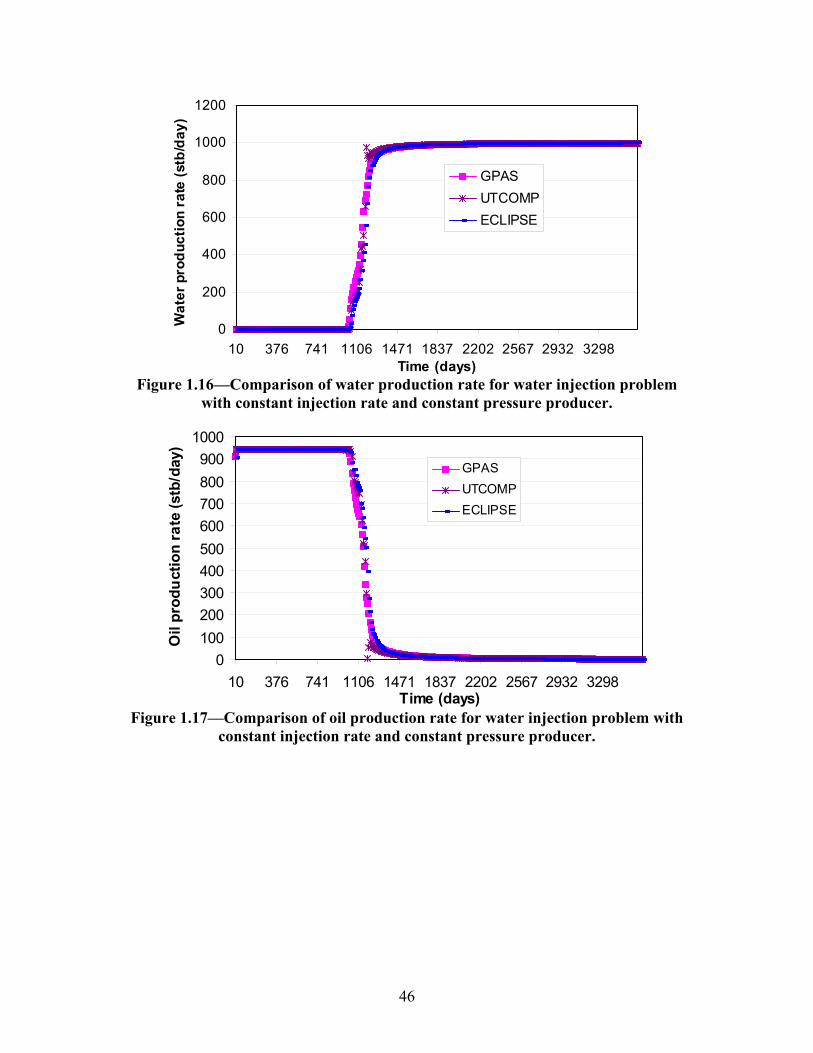
46
0
200
400
600
800
1000
1200
10 376 741 1106 1471 1837 2202 2567 2932 3298Time (days)
Wat
er p
rodu
ctio
n ra
te (s
tb/d
ay)
GPASUTCOMPECLIPSE
Figure 1.16—Comparison of water production rate for water injection problem
with constant injection rate and constant pressure producer.
0100200300400500600700800900
1000
10 376 741 1106 1471 1837 2202 2567 2932 3298Time (days)
Oil
prod
uctio
n ra
te (s
tb/d
ay)
GPASUTCOMPECLIPSE
Figure 1.17—Comparison of oil production rate for water injection problem with
constant injection rate and constant pressure producer.
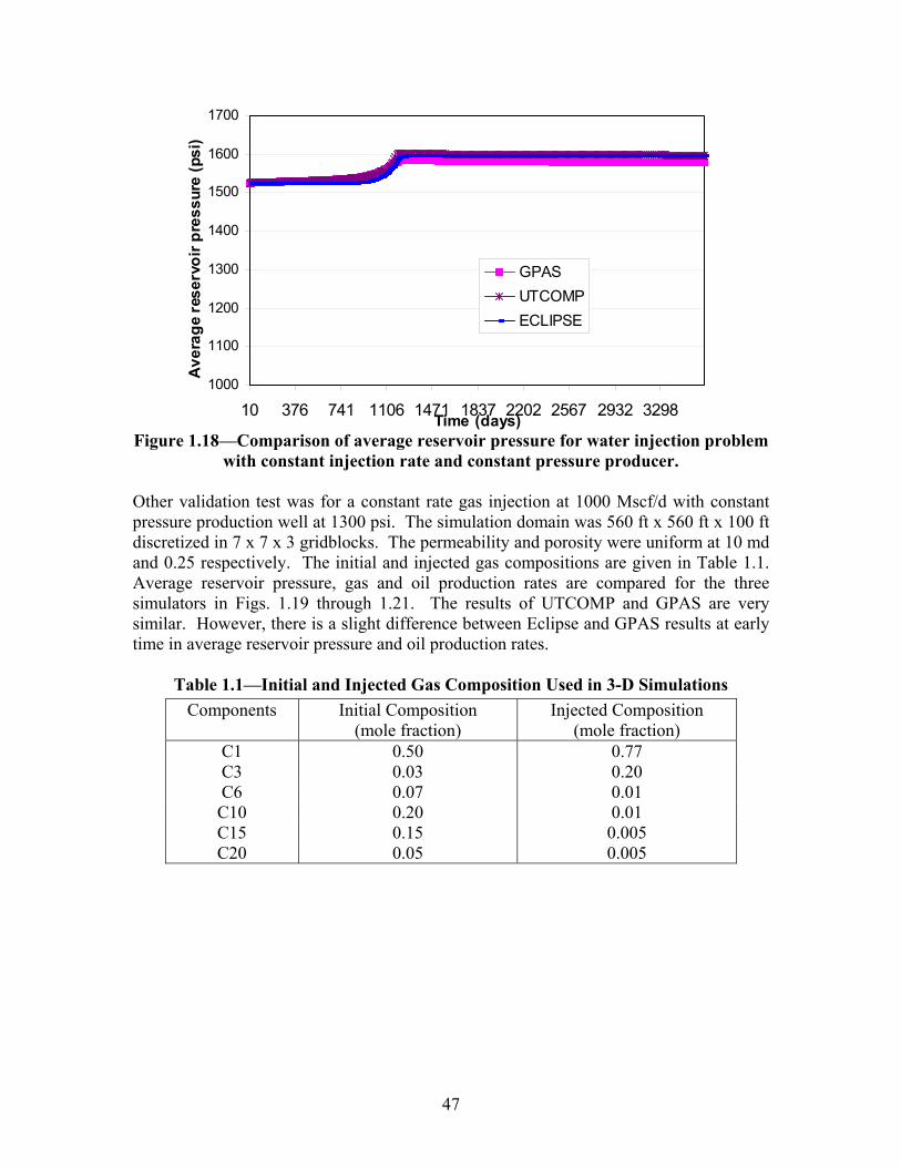
47
1000
1100
1200
1300
1400
1500
1600
1700
10 376 741 1106 1471 1837 2202 2567 2932 3298Time (days)
Ave
rage
res
ervo
ir pr
essu
re (p
si)
GPASUTCOMPECLIPSE
Figure 1.18—Comparison of average reservoir pressure for water injection problem
with constant injection rate and constant pressure producer. Other validation test was for a constant rate gas injection at 1000 Mscf/d with constant pressure production well at 1300 psi. The simulation domain was 560 ft x 560 ft x 100 ft discretized in 7 x 7 x 3 gridblocks. The permeability and porosity were uniform at 10 md and 0.25 respectively. The initial and injected gas compositions are given in Table 1.1. Average reservoir pressure, gas and oil production rates are compared for the three simulators in Figs. 1.19 through 1.21. The results of UTCOMP and GPAS are very similar. However, there is a slight difference between Eclipse and GPAS results at early time in average reservoir pressure and oil production rates.
Table 1.1—Initial and Injected Gas Composition Used in 3-D SimulationsComponents Initial Composition
(mole fraction) Injected Composition
(mole fraction) C1 0.50 0.77 C3 0.03 0.20 C6 0.07 0.01 C10 0.20 0.01 C15 0.15 0.005 C20 0.05 0.005
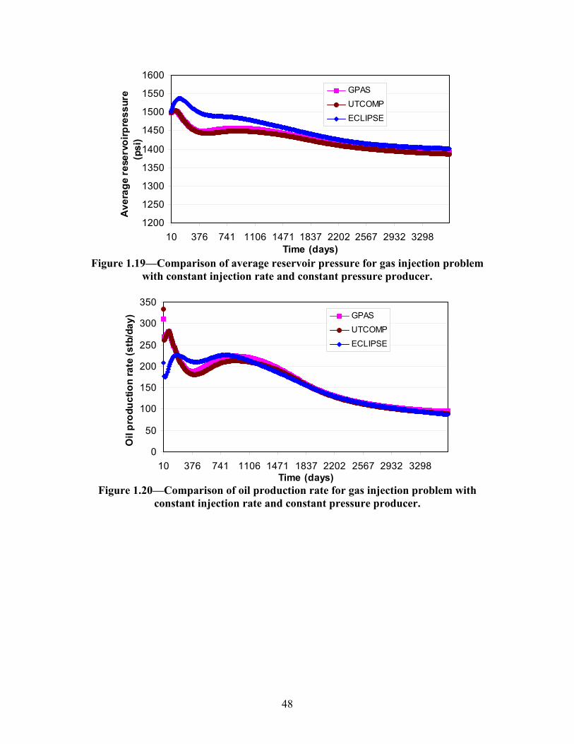
48
1200
1250
1300
1350
1400
1450
1500
1550
1600
10 376 741 1106 1471 1837 2202 2567 2932 3298Time (days)
Ave
rage
res
ervo
irpre
ssur
e (p
si)
GPASUTCOMP
ECLIPSE
Figure 1.19—Comparison of average reservoir pressure for gas injection problem
with constant injection rate and constant pressure producer.
0
50
100
150
200
250
300
350
10 376 741 1106 1471 1837 2202 2567 2932 3298Time (days)
Oil
prod
uctio
n ra
te (s
tb/d
ay) GPAS
UTCOMP
ECLIPSE
Figure 1.20—Comparison of oil production rate for gas injection problem with
constant injection rate and constant pressure producer.
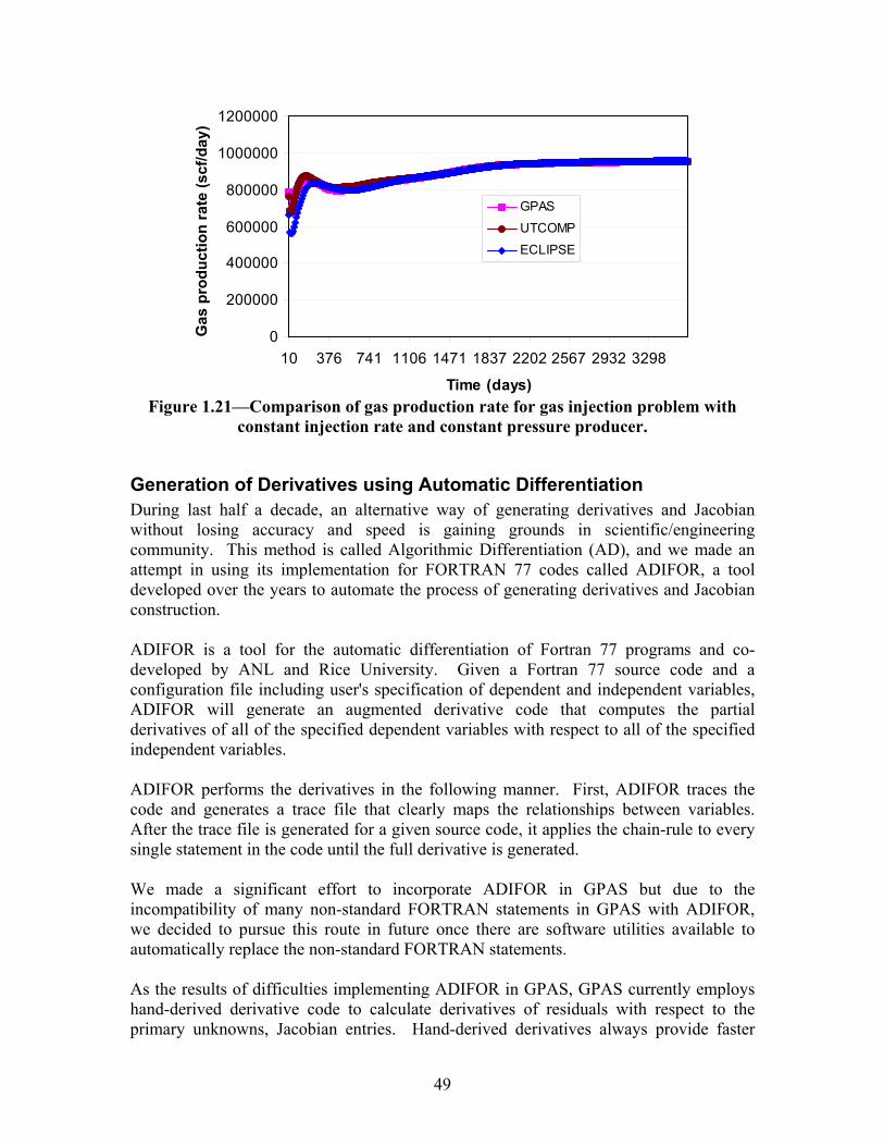
49
0
200000
400000
600000
800000
1000000
1200000
10 376 741 1106 1471 1837 2202 2567 2932 3298
Time (days)
Gas
pro
duct
ion
rate
(scf
/day
)GPAS
UTCOMP
ECLIPSE
Figure 1.21—Comparison of gas production rate for gas injection problem with
constant injection rate and constant pressure producer.
Generation of Derivatives using Automatic Differentiation During last half a decade, an alternative way of generating derivatives and Jacobian without losing accuracy and speed is gaining grounds in scientific/engineering community. This method is called Algorithmic Differentiation (AD), and we made an attempt in using its implementation for FORTRAN 77 codes called ADIFOR, a tool developed over the years to automate the process of generating derivatives and Jacobian construction. ADIFOR is a tool for the automatic differentiation of Fortran 77 programs and co-developed by ANL and Rice University. Given a Fortran 77 source code and a configuration file including user's specification of dependent and independent variables, ADIFOR will generate an augmented derivative code that computes the partial derivatives of all of the specified dependent variables with respect to all of the specified independent variables. ADIFOR performs the derivatives in the following manner. First, ADIFOR traces the code and generates a trace file that clearly maps the relationships between variables. After the trace file is generated for a given source code, it applies the chain-rule to every single statement in the code until the full derivative is generated. We made a significant effort to incorporate ADIFOR in GPAS but due to the incompatibility of many non-standard FORTRAN statements in GPAS with ADIFOR, we decided to pursue this route in future once there are software utilities available to automatically replace the non-standard FORTRAN statements. As the results of difficulties implementing ADIFOR in GPAS, GPAS currently employs hand-derived derivative code to calculate derivatives of residuals with respect to the primary unknowns, Jacobian entries. Hand-derived derivatives always provide faster
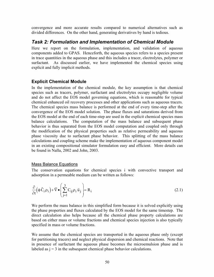
50
convergence and more accurate results compared to numerical alternatives such as divided differences. On the other hand, generating derivatives by hand is tedious.
Task 2: Formulation and Implementation of Chemical Module Here we report on the formulation, implementation, and validation of aqueous components added to GPAS. Henceforth, the aqueous species refers to a species present in trace quantities in the aqueous phase and this includes a tracer, electrolytes, polymer or surfactant. As discussed earlier, we have implemented the chemical species using explicit and fully implicit methods.
Explicit Chemical Module In the implementation of the chemical module, the key assumption is that chemical species such as tracers, polymer, surfactant and electrolytes occupy negligible volume and do not affect the EOS model governing equations, which is reasonable for typical chemical enhanced oil recovery processes and other applications such as aqueous tracers. The chemical species mass balance is performed at the end of every time-step after the convergence of the EOS model solution. The phase fluxes and saturations derived from the EOS model at the end of each time-step are used in the explicit chemical species mass balance calculations. The computation of the mass balance and subsequent phase behavior is thus separated from the EOS model computation and coupled only through the modification of the physical properties such as relative permeability and aqueous phase viscosity due to surfactant phase behavior. This splitting of the mass balance calculations and coupling scheme make the implementation of aqueous component model in an existing compositional simulator formulation easy and efficient. More details can be found in Nalla, 2002 and John, 2003.
Mass Balance Equations The conservation equations for chemical species i with convective transport and adsorption in a permeable medium can be written as follows:
( )3
i i ij i j ij 1
C C u Rt =
∂ φ ρ + ∇ • ρ = ∂ ∑ (2.1)
We perform the mass balance in this simplified form because it is solved explicitly using the phase properties and fluxes calculated by the EOS model for the same timestep. The direct calculation also helps because all the chemical phase property calculations are based on either mass or volume fractions and chemical species injection is also typically specified in mass or volume fractions. We assume that the chemical species are transported in the aqueous phase only (except for partitioning tracers) and neglect physical dispersion and chemical reactions. Note that in presence of surfactant the aqueous phase becomes the microemulsion phase and is labeled as j = 3 in the subsequent chemical phase behavior calculations.
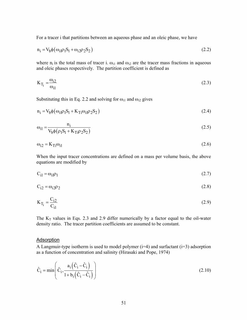
51
For a tracer i that partitions between an aqueous phase and an oleic phase, we have
( )i b i1 1 1 i2 2 2n V S S= φ ω ρ + ω ρ (2.2) where ni is the total mass of tracer i. ωi1 and ωi2 are the tracer mass fractions in aqueous and oleic phases respectively. The partition coefficient is defined as
ii2
Ti1
K ω=
ω (2.3)
Substituting this in Eq. 2.2 and solving for ωi1 and ωi2 gives
( )i b i1 1 1 Ti i1 2 2n V S K S= φ ω ρ + ω ρ (2.4)
( )i
i1b 1 1 Ti 2 2
nV S K S
ω =φ ρ + ρ
(2.5)
i2 Ti i1Kω = ω (2.6)
When the input tracer concentrations are defined on a mass per volume basis, the above equations are modified by
i1 i1 1C = ω ρ (2.7)
i2 i2 2C = ω ρ (2.8)
ii2
Ti1
CKC
= (2.9)
The KT values in Eqs. 2.3 and 2.9 differ numerically by a factor equal to the oil-water density ratio. The tracer partition coefficients are assumed to be constant.
Adsorption A Langmuir-type isotherm is used to model polymer (i=4) and surfactant (i=3) adsorption as a function of concentration and salinity (Hirasaki and Pope, 1974)
( )( )
i i ii i
i i i
ˆa C CC min C ,
ˆ1 b C C
− = + −
(2.10)
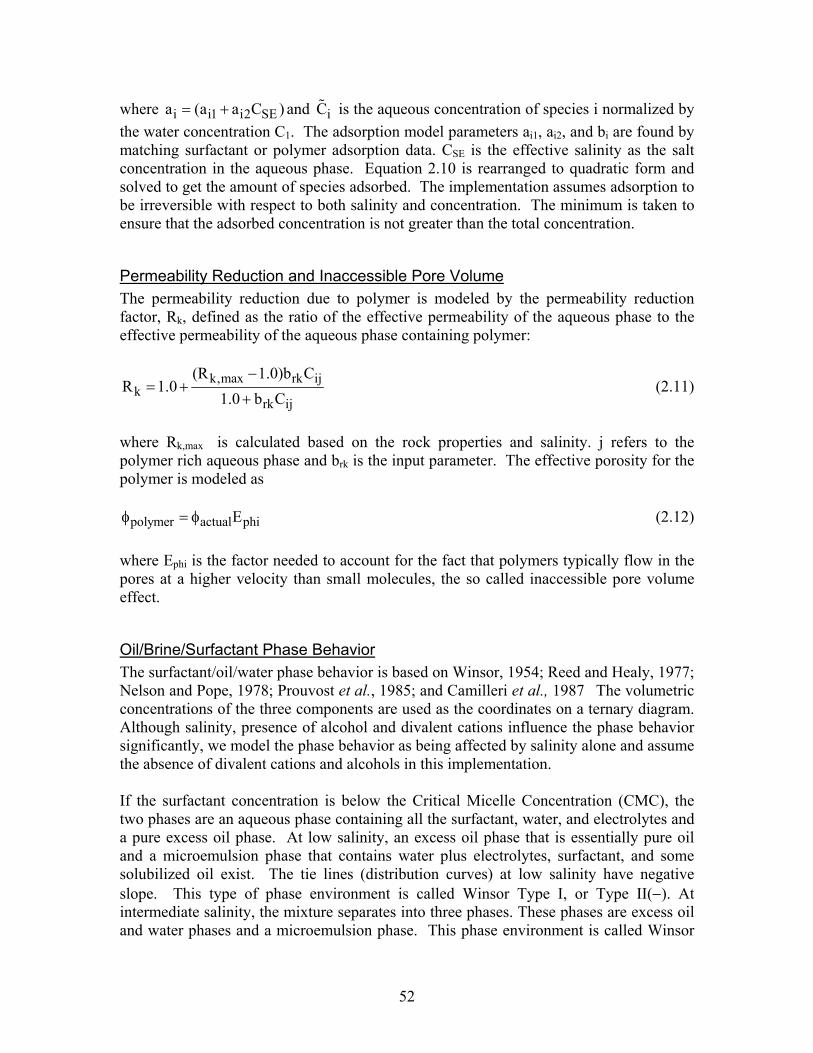
52
where i i1 i2 SEa (a a C )= + and iC is the aqueous concentration of species i normalized by the water concentration C1. The adsorption model parameters ai1, ai2, and bi are found by matching surfactant or polymer adsorption data. CSE is the effective salinity as the salt concentration in the aqueous phase. Equation 2.10 is rearranged to quadratic form and solved to get the amount of species adsorbed. The implementation assumes adsorption to be irreversible with respect to both salinity and concentration. The minimum is taken to ensure that the adsorbed concentration is not greater than the total concentration.
Permeability Reduction and Inaccessible Pore Volume The permeability reduction due to polymer is modeled by the permeability reduction factor, Rk, defined as the ratio of the effective permeability of the aqueous phase to the effective permeability of the aqueous phase containing polymer:
k,max rk ijk
rk ij
(R 1.0)b CR 1.0
1.0 b C−
= ++
(2.11)
where Rk,max is calculated based on the rock properties and salinity. j refers to the polymer rich aqueous phase and brk is the input parameter. The effective porosity for the polymer is modeled as
polymer actual phiEφ = φ (2.12) where Ephi is the factor needed to account for the fact that polymers typically flow in the pores at a higher velocity than small molecules, the so called inaccessible pore volume effect.
Oil/Brine/Surfactant Phase Behavior The surfactant/oil/water phase behavior is based on Winsor, 1954; Reed and Healy, 1977; Nelson and Pope, 1978; Prouvost et al., 1985; and Camilleri et al., 1987 The volumetric concentrations of the three components are used as the coordinates on a ternary diagram. Although salinity, presence of alcohol and divalent cations influence the phase behavior significantly, we model the phase behavior as being affected by salinity alone and assume the absence of divalent cations and alcohols in this implementation. If the surfactant concentration is below the Critical Micelle Concentration (CMC), the two phases are an aqueous phase containing all the surfactant, water, and electrolytes and a pure excess oil phase. At low salinity, an excess oil phase that is essentially pure oil and a microemulsion phase that contains water plus electrolytes, surfactant, and some solubilized oil exist. The tie lines (distribution curves) at low salinity have negative slope. This type of phase environment is called Winsor Type I, or Type II(−). At intermediate salinity, the mixture separates into three phases. These phases are excess oil and water phases and a microemulsion phase. This phase environment is called Winsor

53
Type III, or just Type III. At high salinity, an excess water phase and a microemulsion phase containing most of the surfactant and oil, and some solubilized water exist. This type of phase environment is called Winsor Type II, or alternatively Type II(+). Other variables besides electrolyte concentrations, e.g. alcohol type and concentration, the equivalent alkane carbon number of the oil or solvent and changes in temperature or pressure also cause a phase environment shift from one type of phase behavior to another type but these effects are not modeled here. The surfactant/oil/water phase behavior is thus represented as a function of effective salinity once the binodal curve and tie lines are described. The oil concentrations used in the calculations are obtained from the EOS model at the end of each converged time step. Since they belong to the EOS model, they cannot be changed during the explicit chemical phase behavior calculations. This coupling forces the assumption of negligible changes in oil saturation due to solubilization. The surfactant phase behavior is therefore limited to Type II(-) behavior with microemulsion and oil as the two phases in equilibrium in this implementation with the following assumptions:
• isothermal conditions, • corner plait point formulation where the excess oil phase is pure oil phase, • binodal curve formulation based on Hand’s rule (Hand, 1939), • a symmetric binodal curve, • no effect of divalent cations such as calcium or alcohol on phase behavior, • the phase behavior is independent of the polymer concentration, • no gas is present, and • no effect of pressure on microemulsion phase behavior.
Hand’s rule is based on the empirical observation that equilibrium phase concentration ratios are straight lines on a log-log scale. The binodal curve is described by
13j 3j
2 j 1j
C CA for j 2, 3
C C
−
= =
(2.13)
The parameter A is related to the height of binodal curve as follows:
23max,s
s3max,s
2CA for s 0, 1
1 C
= = − (2.14)
where s = 0, 1 represents the zero and optimal salinities. Linear interpolation is used to determine the A parameter for intermediate salinities.
( ) SE0 1 1 SE SEOP
SEOP
CA A A 1 A for C CC
= − − + ≤
(2.15)
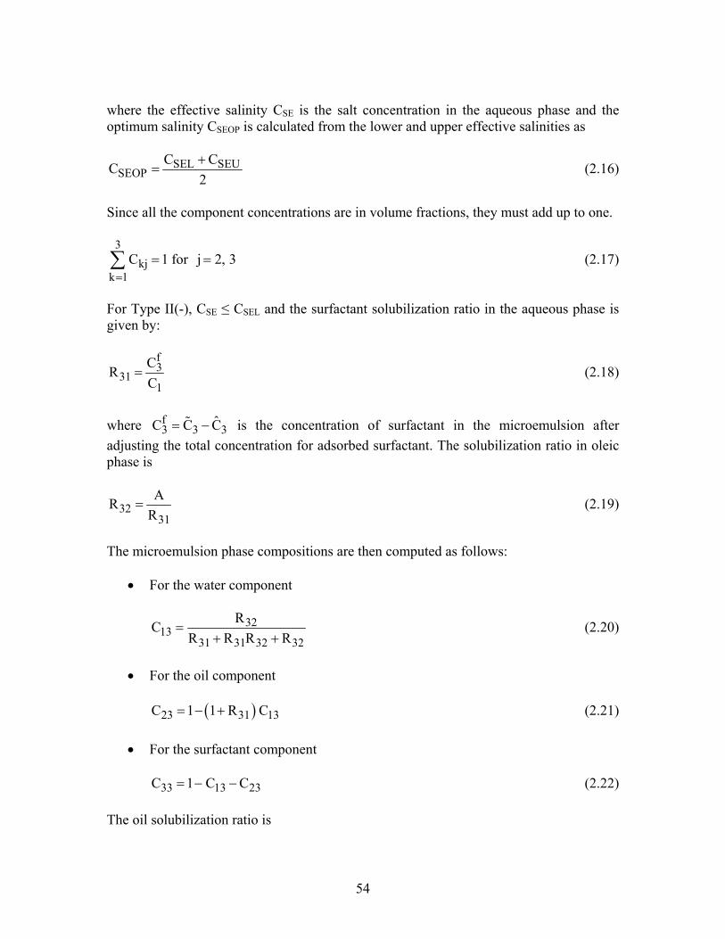
54
where the effective salinity CSE is the salt concentration in the aqueous phase and the optimum salinity CSEOP is calculated from the lower and upper effective salinities as
SEL SEUSEOP
C CC2+
= (2.16)
Since all the component concentrations are in volume fractions, they must add up to one.
3kj
k 1C 1 for j 2, 3
== =∑ (2.17)
For Type II(-), CSE ≤ CSEL and the surfactant solubilization ratio in the aqueous phase is given by:
f3
311
CRC
= (2.18)
where f
3 3 3ˆC C C= − is the concentration of surfactant in the microemulsion after adjusting the total concentration for adsorbed surfactant. The solubilization ratio in oleic phase is
3231
ARR
= (2.19)
The microemulsion phase compositions are then computed as follows:
• For the water component
3213
31 31 32 32
RCR R R R
=+ +
(2.20)
• For the oil component
( )23 31 13C 1 1 R C= − + (2.21)
• For the surfactant component 33 13 23C 1 C C= − − (2.22) The oil solubilization ratio is
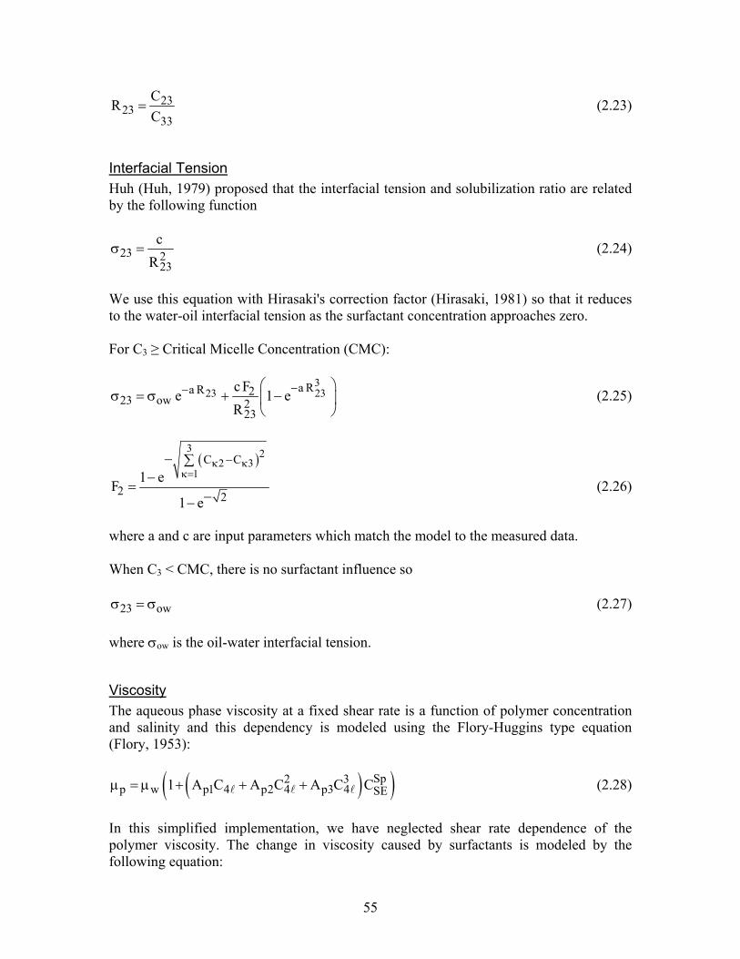
55
2323
33
CRC
= (2.23)
Interfacial Tension Huh (Huh, 1979) proposed that the interfacial tension and solubilization ratio are related by the following function
23 223
cR
σ = (2.24)
We use this equation with Hirasaki's correction factor (Hirasaki, 1981) so that it reduces to the water-oil interfacial tension as the surfactant concentration approaches zero. For C3 ≥ Critical Micelle Concentration (CMC):
323 23a Ra R 2
23 ow 223
c Fe 1 eR
−− σ = σ + −
(2.25)
( )3 2
2 31
C C
2 21 eF
1 e
κ κκ=
−− ∑−
=−−
(2.26)
where a and c are input parameters which match the model to the measured data. When C3 < CMC, there is no surfactant influence so
23 owσ = σ (2.27) where σow is the oil-water interfacial tension.
Viscosity The aqueous phase viscosity at a fixed shear rate is a function of polymer concentration and salinity and this dependency is modeled using the Flory-Huggins type equation (Flory, 1953):
( )( )Sp2 3p w p1 4 p2 4 p3 4 SE1 A C A C A C Cµ = µ + + + (2.28)
In this simplified implementation, we have neglected shear rate dependence of the polymer viscosity. The change in viscosity caused by surfactants is modeled by the following equation:
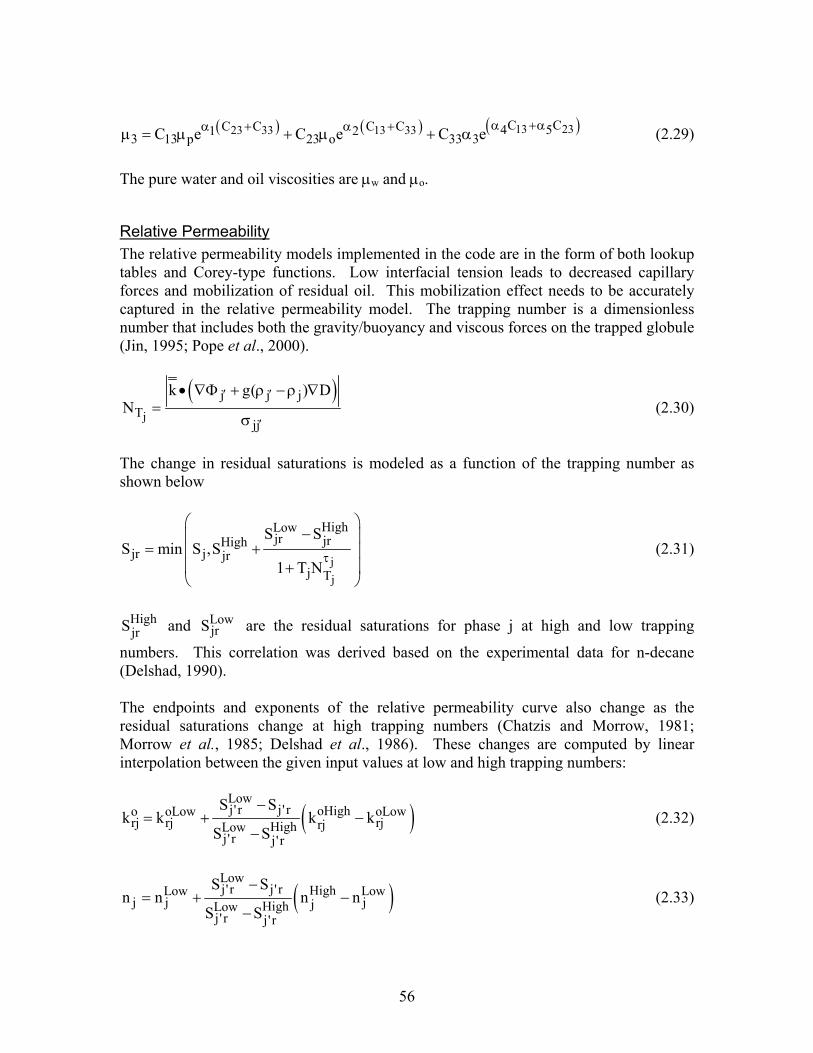
56
( ) ( ) ( )13 2323 33 13 33 C CC C C C 4 51 23 13 p 23 o 33 3C e C e C e α +αα + α +µ = µ + µ + α (2.29)
The pure water and oil viscosities are µw and µo.
Relative Permeability The relative permeability models implemented in the code are in the form of both lookup tables and Corey-type functions. Low interfacial tension leads to decreased capillary forces and mobilization of residual oil. This mobilization effect needs to be accurately captured in the relative permeability model. The trapping number is a dimensionless number that includes both the gravity/buoyancy and viscous forces on the trapped globule (Jin, 1995; Pope et al., 2000).
( )j
j j jT
jj
k g( ) DN
′ ′
′
• ∇Φ + ρ − ρ ∇=
σ (2.30)
The change in residual saturations is modeled as a function of the trapping number as shown below
jj
HighLowjr jrHigh
jr j jrj T
S SS min S ,S
1 T Nτ
−
= + +
(2.31)
HighjrS and Low
jrS are the residual saturations for phase j at high and low trapping
numbers. This correlation was derived based on the experimental data for n-decane (Delshad, 1990). The endpoints and exponents of the relative permeability curve also change as the residual saturations change at high trapping numbers (Chatzis and Morrow, 1981; Morrow et al., 1985; Delshad et al., 1986). These changes are computed by linear interpolation between the given input values at low and high trapping numbers:
( )Lowj' r j' r oHigho oLow oLow
rj rj rjrjHighLowj' r j' r
S Sk k k k
S S
−= + −
− (2.32)
( )Lowj' r j' r HighLow Low
j j jjHighLowj' r j' r
S Sn n n n
S S
−= + −
− (2.33)
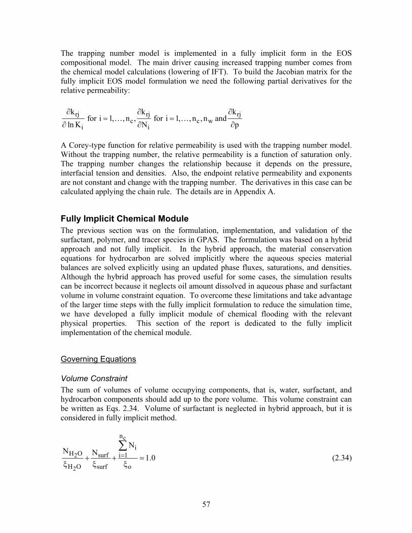
57
The trapping number model is implemented in a fully implicit form in the EOS compositional model. The main driver causing increased trapping number comes from the chemical model calculations (lowering of IFT). To build the Jacobian matrix for the fully implicit EOS model formulation we need the following partial derivatives for the relative permeability:
rj rj rjc c w
i i
k k kfor i 1, , n , for i 1, , n , n and
ln K N p∂ ∂ ∂
= =∂ ∂ ∂
… …
A Corey-type function for relative permeability is used with the trapping number model. Without the trapping number, the relative permeability is a function of saturation only. The trapping number changes the relationship because it depends on the pressure, interfacial tension and densities. Also, the endpoint relative permeability and exponents are not constant and change with the trapping number. The derivatives in this case can be calculated applying the chain rule. The details are in Appendix A.
Fully Implicit Chemical Module The previous section was on the formulation, implementation, and validation of the surfactant, polymer, and tracer species in GPAS. The formulation was based on a hybrid approach and not fully implicit. In the hybrid approach, the material conservation equations for hydrocarbon are solved implicitly where the aqueous species material balances are solved explicitly using an updated phase fluxes, saturations, and densities. Although the hybrid approach has proved useful for some cases, the simulation results can be incorrect because it neglects oil amount dissolved in aqueous phase and surfactant volume in volume constraint equation. To overcome these limitations and take advantage of the larger time steps with the fully implicit formulation to reduce the simulation time, we have developed a fully implicit module of chemical flooding with the relevant physical properties. This section of the report is dedicated to the fully implicit implementation of the chemical module.
Governing Equations
Volume Constraint The sum of volumes of volume occupying components, that is, water, surfactant, and hydrocarbon components should add up to the pore volume. This volume constraint can be written as Eqs. 2.34. Volume of surfactant is neglected in hybrid approach, but it is considered in fully implicit method.
c
2
2
n
iH O surf i 1
H O surf o
NN N 1.0=+ + =ξ ξ ξ
∑ (2.34)
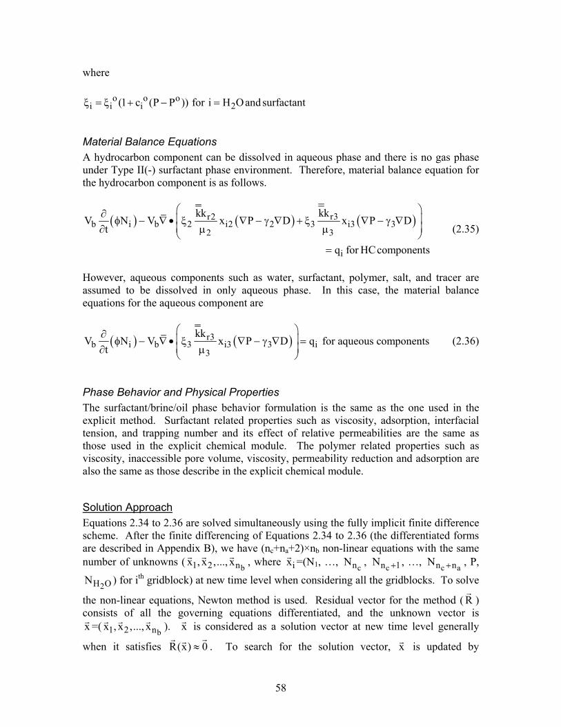
58
where
o o oi i i 2(1 c (P P )) for i H Oandsurfactantξ = ξ + − =
Material Balance Equations A hydrocarbon component can be dissolved in aqueous phase and there is no gas phase under Type II(-) surfactant phase environment. Therefore, material balance equation for the hydrocarbon component is as follows.
( ) ( ) ( )r3r2b i b 2 i2 2 3 i3 3
2 3
i
kkkkV N V x P D x P D
t
q for HCcomponents
∂ φ − ∇ • ξ ∇ − γ ∇ + ξ ∇ − γ ∇ ∂ µ µ
=
(2.35)
However, aqueous components such as water, surfactant, polymer, salt, and tracer are assumed to be dissolved in only aqueous phase. In this case, the material balance equations for the aqueous component are
( ) ( )r3b i b 3 i3 3 i
3
kkV N V x P D q for aqueous components
t
∂ φ − ∇ • ξ ∇ − γ ∇ = ∂ µ
(2.36)
Phase Behavior and Physical Properties The surfactant/brine/oil phase behavior formulation is the same as the one used in the explicit method. Surfactant related properties such as viscosity, adsorption, interfacial tension, and trapping number and its effect of relative permeabilities are the same as those used in the explicit chemical module. The polymer related properties such as viscosity, inaccessible pore volume, viscosity, permeability reduction and adsorption are also the same as those describe in the explicit chemical module.
Solution Approach Equations 2.34 to 2.36 are solved simultaneously using the fully implicit finite difference scheme. After the finite differencing of Equations 2.34 to 2.36 (the differentiated forms are described in Appendix B), we have (nc+na+2)×nb non-linear equations with the same number of unknowns ( b1 2 nx , x ,..., x , where ix =(N1, …, cnN , cn 1N + , …, c an nN + , P,
2H ON ) for ith gridblock) at new time level when considering all the gridblocks. To solve
the non-linear equations, Newton method is used. Residual vector for the method ( R ) consists of all the governing equations differentiated, and the unknown vector is x =( b1 2 nx , x ,..., x ). x is considered as a solution vector at new time level generally
when it satisfies R(x) 0≈ . To search for the solution vector, x is updated by
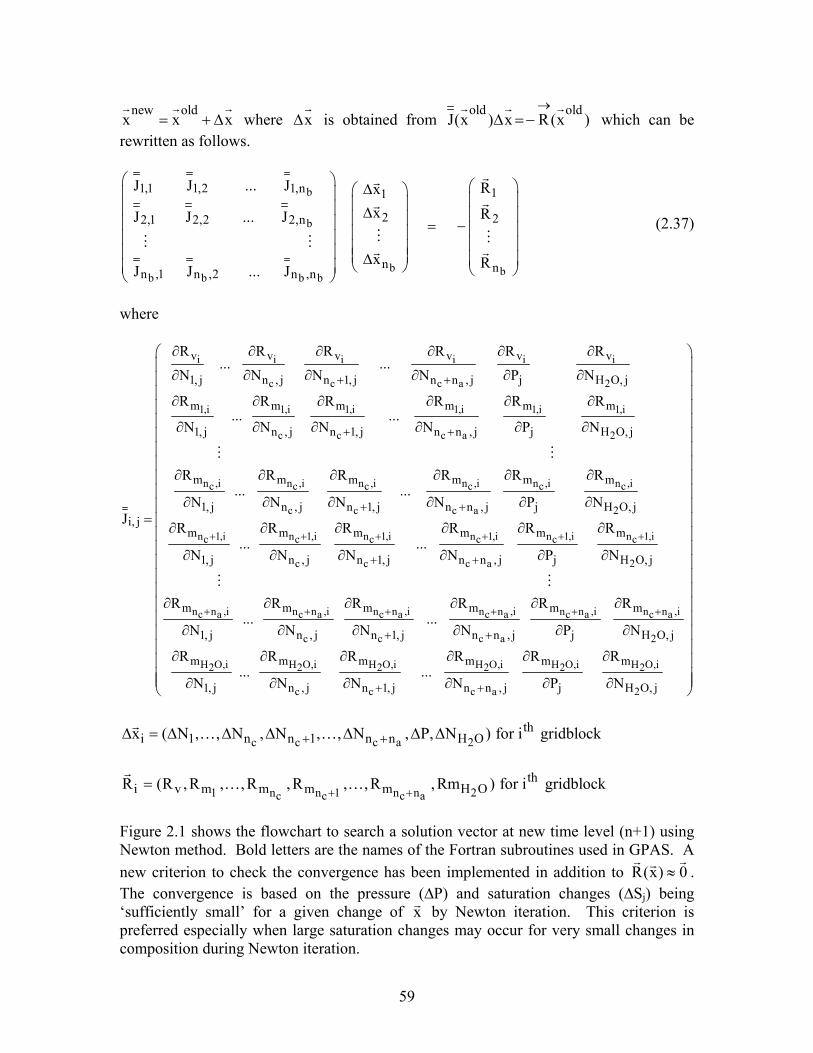
59
new oldx x x= + ∆ where x∆ is obtained from
old oldJ(x ) x R(x )
→∆ = − which can be
rewritten as follows.
b
b
b bb b b b
1,1 1,2 1,n 11
2 22,1 2,2 2,n
n nn ,1 n ,2 n ,n
J J ... J Rxx RJ J ... J
x RJ J ... J
∆ ∆ = − ∆
(2.37)
where
i i i i i i
c c c a 2
1,i 1,i 1,i 1,i 1,i 1,i
c c c a 2
n ,i n ,i n ,ic c c
c c
v v v v v v
1, j n , j n 1, j n n , j j H O, j
m m m m m m
1, j n , j n 1, j n n , j j H O, j
m m m
1, j n , j n 1, ji, j
R R R R R R... ...
N N N N P N
R R R R R R... ...
N N N N P N
R R R... ..
N N NJ
+ +
+ +
+
∂ ∂ ∂ ∂ ∂ ∂
∂ ∂ ∂ ∂ ∂ ∂
∂ ∂ ∂ ∂ ∂ ∂
∂ ∂ ∂ ∂ ∂ ∂
∂ ∂ ∂
∂ ∂ ∂=
n ,i n ,i n ,ic c c
c a 2
n 1,i n 1,i n 1,i n 1,i n 1,i n 1,ic c c c c c
c c c a 2
n n ,i n n ,i n n ,i nc a c a c a
c c
m m m
n n , j j H O, j
m m m m m m
1, j n , j n 1, j n n , j j H O, j
m m m m
1, j n , j n 1, j
R R R.
N P N
R R R R R R... ...
N N N N P N
R R R R... ...
N N N
+ + + + + +
+ + +
+
+ +
+
∂ ∂ ∂
∂ ∂ ∂
∂ ∂ ∂ ∂ ∂ ∂
∂ ∂ ∂ ∂ ∂ ∂
∂ ∂ ∂ ∂
∂ ∂ ∂n ,i n n ,i n n ,ic a c a c a
c a 2
H O,i H O,i H O,i H O,i H O,i H O,i2 2 2 2 2 2
c c c a 2
m m
n n , j j H O, j
m m m m m m
1, j n , j n 1, j n n , j j H O, j
R R
N P N
R R R R R R... ...
N N N N P N
+ + +
+
+ +
∂ ∂
∂ ∂ ∂ ∂ ∂ ∂ ∂ ∂ ∂ ∂ ∂ ∂ ∂ ∂ ∂
c c c a 2th
i 1 n n 1 n n H Ox ( N , , N , N , , N , P, N ) for i gridblock+ +∆ = ∆ ∆ ∆ ∆ ∆ ∆… …
1 n n 1 n n 2c c c ath
i v m m m m H OR (R ,R , ,R ,R , ,R ,Rm ) for i gridblock+ +
= … …
Figure 2.1 shows the flowchart to search a solution vector at new time level (n+1) using Newton method. Bold letters are the names of the Fortran subroutines used in GPAS. A new criterion to check the convergence has been implemented in addition to R(x) 0≈ . The convergence is based on the pressure (∆P) and saturation changes (∆Sj) being ‘sufficiently small’ for a given change of x by Newton iteration. This criterion is preferred especially when large saturation changes may occur for very small changes in composition during Newton iteration.
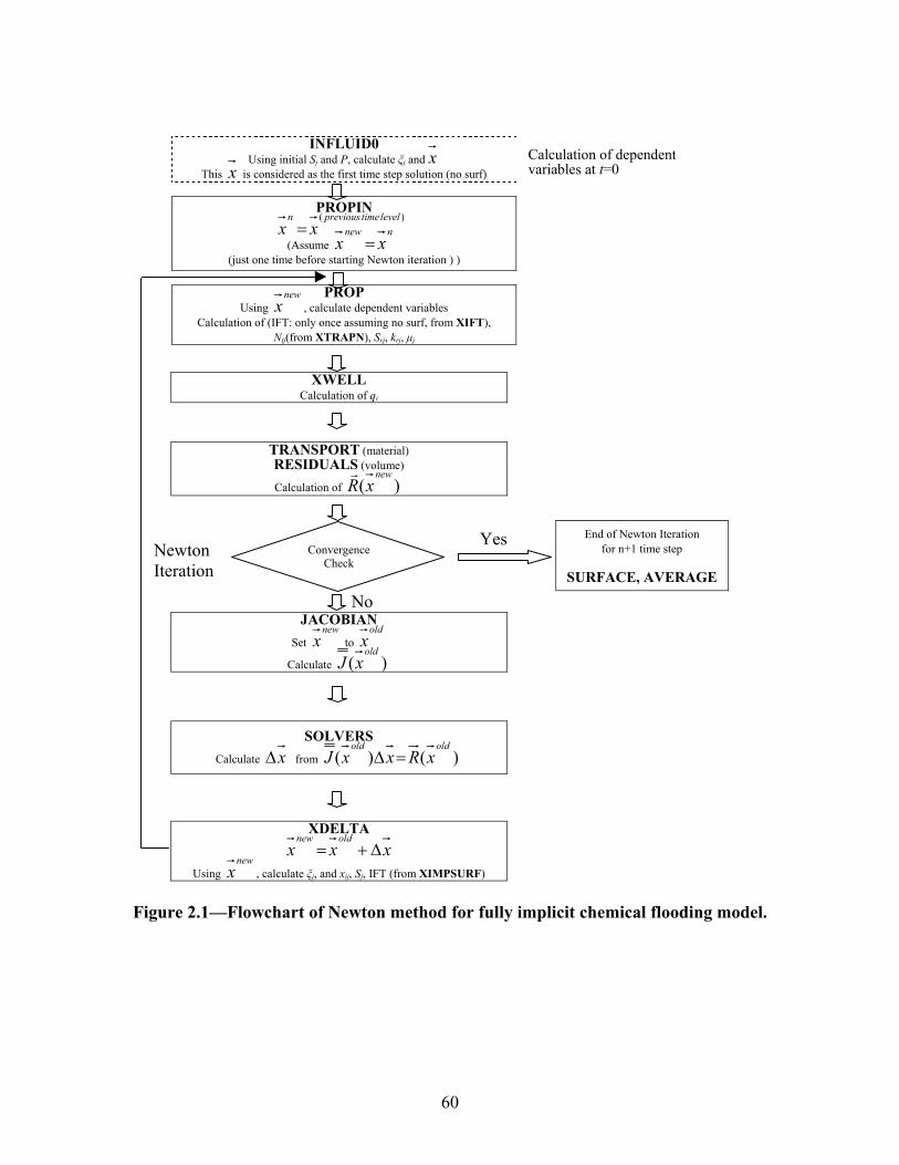
60
INFLUID0
Using initial Sj and P, calculate ξj and x This x is considered as the first time step solution (no surf)
PROPIN
)( leveltimepreviousnxx =
(Assume nnew
xx = (just one time before starting Newton iteration ) )
PROP
Using new
x , calculate dependent variables Calculation of (IFT: only once assuming no surf, from XIFT),
Ntj(from XTRAPN), Srj, krj, µj
XWELL
Calculation of qi
TRANSPORT (material) RESIDUALS (volume)
Calculation of )(new
xR
Convergence
Check
End of Newton Iteration for n+1 time step
SURFACE, AVERAGE
JACOBIAN
Set new
x to old
x
Calculate )(old
xJ
SOLVERS Calculate x∆ from )()(
oldoldxRxxJ =∆
XDELTA xxx
oldnew∆+=
Using new
x , calculate ξj, and xij, Sj, IFT (from XIMPSURF)
Figure 2.1—Flowchart of Newton method for fully implicit chemical flooding model.
Yes
No
Newton Iteration
Calculation of dependent variables at t=0
61
Task 3: Validation and Application Test cases were run on GPAS and the results were compared with both analytical solutions and output from the miscible-gas flooding compositional simulator, UTCOMP (Chang, 1990), or the chemical flooding simulator, UTCHEM (Delshad et al., 1996; Delshad et al., 2002), to check the correctness of the code. The flash algorithm was tested with a batch flash calculation for a binary mixture. A Buckley-Leverett problem was run on GPAS and compared with the analytical solution and output from the chemical flooding simulator UTCHEM. A comparison of the results from GPAS with UTCOMP of an example simulation of carbon dioxide sequestration is also given. The standard SPE fifth comparative solution project (Killough and Kossack, 1987) was modified and simulations were carried out using GPAS and UTCOMP. The comparison of these results from GPAS with UTCOMP for the modified SPE fifth comparative solution project is discussed. We performed a series of 2-D and 3-D surfactant/polymer flood simulations using both the explicit and implicit formulations and have made comparison with UTCHEM simulation results. We have made numerous parallel simulations on up to 128 processors to study the scalability of GPAS. We have made for the first time, a 1000,000 gridblock surfactant/polymer flood simulation on 128 processors.
Batch Flash of Ethane-Propylene Binary Mixture The goal is to verify the correctness of the flash calculations. The mathematical formulation of the flash algorithm is discussed in Task 1. The test case considered here is a mixture of ethane and propylene. The simulation domain dimensions are 5000 ft in length, 500 ft in width and 20 ft in thickness. Since the simulation is a batch flash, there is no well section in the input. The initial composition is 0.5 mole fraction each of ethane and propylene. The details of the input file including the critical properties of the components are given in Table 3.1. The simulation is run for one day. A program for multi-component vapor-liquid equilibrium calculations using the Peng-Robinson cubic equation-of-state, VLMU (Sandler, 1999) was also used as a basis for comparison. UTCOMP and GPAS use the same form of PR EOS while VLMU uses a slightly different form of PR EOS. For acentric factor values less than 0.49, all the three codes use the same equations. The only difference is that GPAS and UTCOMP use a different expression for the calculation of κ (Eqs 1.28 and 1.29) for the acentric factor values greater than 0.49 while VLMU uses the same expression for all values of acentric factors. Since in this test case, the acentric factor for both the components is less than 0.49, all the three codes essentially use the same PR EOS equations. The iteration tolerances in UTCOMP and GPAS are set at 10-8. The volume shift parameter functionality is available in UTCOMP but is not implemented in GPAS and VLMU. Hence the volume shift parameter is set to zero in UTCOMP.
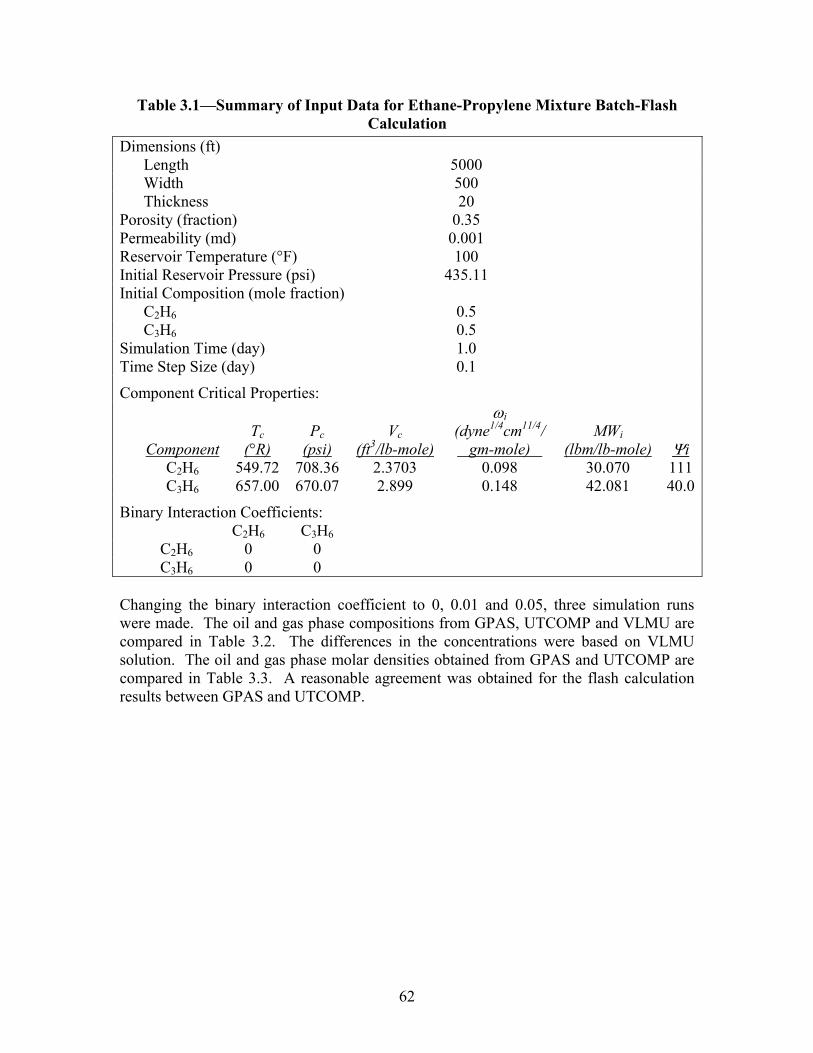
62
Table 3.1—Summary of Input Data for Ethane-Propylene Mixture Batch-Flash Calculation
Dimensions (ft) Length 5000 Width 500 Thickness 20
Porosity (fraction) 0.35 Permeability (md) 0.001 Reservoir Temperature (°F) 100 Initial Reservoir Pressure (psi) 435.11 Initial Composition (mole fraction)
C2H6 0.5 C3H6 0.5
Simulation Time (day) 1.0 Time Step Size (day) 0.1
Component Critical Properties:
Component Tc
(°R) Pc
(psi) Vc
(ft3/lb-mole)
ωi (dyne1/4cm11/4/ gm-mole)
MWi (lbm/lb-mole) Ψi
C2H6 549.72 708.36 2.3703 0.098 30.070 111 C3H6 657.00 670.07 2.899 0.148 42.081 40.0
Binary Interaction Coefficients: C2H6 C3H6 C2H6 0 0 C3H6 0 0 Changing the binary interaction coefficient to 0, 0.01 and 0.05, three simulation runs were made. The oil and gas phase compositions from GPAS, UTCOMP and VLMU are compared in Table 3.2. The differences in the concentrations were based on VLMU solution. The oil and gas phase molar densities obtained from GPAS and UTCOMP are compared in Table 3.3. A reasonable agreement was obtained for the flash calculation results between GPAS and UTCOMP.
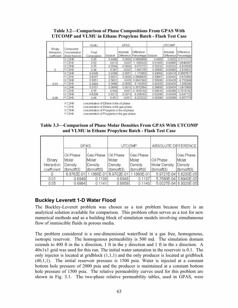
63
Table 3.2—Comparison of Phase Compositions From GPAS With UTCOMP and VLMU in Ethane Propylene Batch - Flash Test Case
Table 3.3—Comparison of Phase Molar Densities From GPAS With UTCOMP and VLMU in Ethane Propylene Batch - Flash Test Case
Buckley Leverett 1-D Water Flood The Buckley-Leverett problem was chosen as a test problem because there is an analytical solution available for comparison. This problem often serves as a test for new numerical methods and as a building block of simulation models involving simultaneous flow of immiscible fluids in porous media. The problem considered is a one-dimensional waterflood in a gas free, homogenous, isotropic reservoir. The homogenous permeability is 500 md. The simulation domain extends to 400 ft in the x direction, 1 ft in the y direction and 1 ft in the z direction. A 40x1x1 grid was used for this run. The initial water saturation in the reservoir is 0.1. The only injector is located at gridblock (1,1,1) and the only producer is located at gridblock (40,1,1). The initial reservoir pressure is 1500 psia. Water is injected at a constant bottom hole pressure of 2000 psia and the producer is maintained at a constant bottom hole pressure of 1500 psia. The relative permeability curves used for this problem are shown in Fig. 3.1. The two-phase relative permeability tables, used in GPAS, were
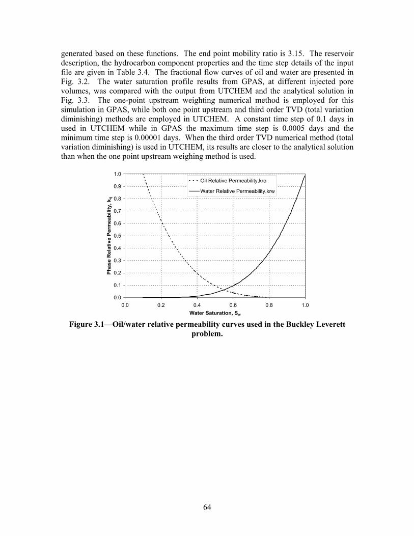
64
generated based on these functions. The end point mobility ratio is 3.15. The reservoir description, the hydrocarbon component properties and the time step details of the input file are given in Table 3.4. The fractional flow curves of oil and water are presented in Fig. 3.2. The water saturation profile results from GPAS, at different injected pore volumes, was compared with the output from UTCHEM and the analytical solution in Fig. 3.3. The one-point upstream weighting numerical method is employed for this simulation in GPAS, while both one point upstream and third order TVD (total variation diminishing) methods are employed in UTCHEM. A constant time step of 0.1 days in used in UTCHEM while in GPAS the maximum time step is 0.0005 days and the minimum time step is 0.00001 days. When the third order TVD numerical method (total variation diminishing) is used in UTCHEM, its results are closer to the analytical solution than when the one point upstream weighing method is used.
0.0
0.1
0.2
0.3
0.4
0.5
0.6
0.7
0.8
0.9
1.0
0.0 0.2 0.4 0.6 0.8 1.0Water Saturation, Sw
Phas
e R
elat
ive
Perm
eabi
lity,
krj
Oil Relative Permeability,kro
Water Relative Permeability,krw
Figure 3.1—Oil/water relative permeability curves used in the Buckley Leverett
problem.
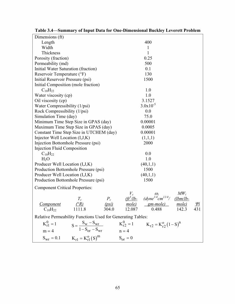
65
Table 3.4—Summary of Input Data for One-Dimensional Buckley Leverett Problem Dimensions (ft)
Length 400 Width 1 Thickness 1
Porosity (fraction) 0.25 Permeability (md) 500 Initial Water Saturation (fraction) 0.1 Reservoir Temperature (°F) 130 Initial Reservoir Pressure (psi) 1500 Initial Composition (mole fraction)
C10H22 1.0 Water viscosity (cp) 1.0 Oil viscosity (cp) 3.1527 Water Compressibility (1/psi) 3.0x10⁻⁵ Rock Compressibility (1/psi) 0.0 Simulation Time (day) 75.0 Minimum Time Step Size in GPAS (day) 0.00001 Maximum Time Step Size in GPAS (day) 0.0005 Constant Time Step Size in UTCHEM (day) 0.00001 Injector Well Location (I,J,K) (1,1,1) Injection Bottomhole Pressure (psi) 2000 Injection Fluid Composition
C10H22 0.0 H2O 1.0
Producer Well Location (I,J,K) (40,1,1) Production Bottomhole Pressure (psi) 1500 Producer Well Location (I,J,K) (40,1,1) Production Bottomhole Pressure (psi) 1500
Component Critical Properties:
Component Tc
(°R) Pc
(psi)
Vc (ft3/lb-mole)
ωi (dyne1/4cm11/4/ gm-mole)
MWi (lbm/lb-mole) Ψi
C10H22 1111.8 304.0 12.087 0.488 142.3 431
Relative Permeability Functions Used for Generating Tables: 0
r1
wr
K 1m 4S 0.1
==
=
( )
w wr
or wrmo
r1 r1
S SS
1 S S
K K S
−=
− −
=
0r2
or
K 1n 4S 0
==
=
( )nor2 r2K K 1 S= −
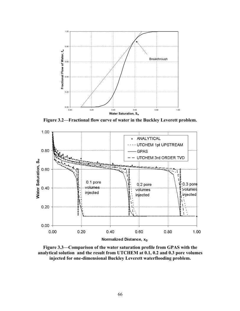
66
0.00
0.20
0.40
0.60
0.80
1.00
0.00 0.20 0.40 0.60 0.80 1.00
Water Saturation, Sw
Frac
tiona
l Flo
w o
f Wat
er, f
w
Breakthrough
Figure 3.2—Fractional flow curve of water in the Buckley Leverett problem.
Figure 3.3—Comparison of the water saturation profile from GPAS with the
analytical solution and the result from UTCHEM at 0.1, 0.2 and 0.3 pore volumes injected for one-dimensional Buckley Leverett waterflooding problem.
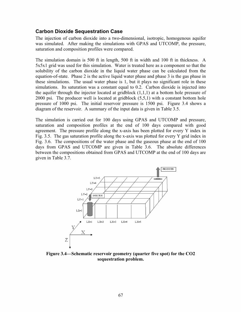
67
Carbon Dioxide Sequestration Case The injection of carbon dioxide into a two-dimensional, isotropic, homogenous aquifer was simulated. After making the simulations with GPAS and UTCOMP, the pressure, saturation and composition profiles were compared. The simulation domain is 500 ft in length, 500 ft in width and 100 ft in thickness. A 5x5x1 grid was used for this simulation. Water is treated here as a component so that the solubility of the carbon dioxide in the liquid water phase can be calculated from the equation-of-state. Phase 2 is the active liquid water phase and phase 3 is the gas phase in these simulations. The usual water phase is 1, but it plays no significant role in these simulations. Its saturation was a constant equal to 0.2. Carbon dioxide is injected into the aquifer through the injector located at gridblock (1,1,1) at a bottom hole pressure of 2000 psi. The producer well is located at gridblock (5,5,1) with a constant bottom hole pressure of 1000 psi. The initial reservoir pressure is 1500 psi. Figure 3.4 shows a diagram of the reservoir. A summary of the input data is given in Table 3.5. The simulation is carried out for 100 days using GPAS and UTCOMP and pressure, saturation and composition profiles at the end of 100 days compared with good agreement. The pressure profile along the x-axis has been plotted for every Y index in Fig. 3.5. The gas saturation profile along the x-axis was plotted for every Y grid index in Fig. 3.6. The compositions of the water phase and the gaseous phase at the end of 100 days from GPAS and UTCOMP are given in Table 3.6. The absolute differences between the compositions obtained from GPAS and UTCOMP at the end of 100 days are given in Table 3.7.
Figure 3.4—Schematic reservoir geometry (quarter five spot) for the CO2
sequestration problem.
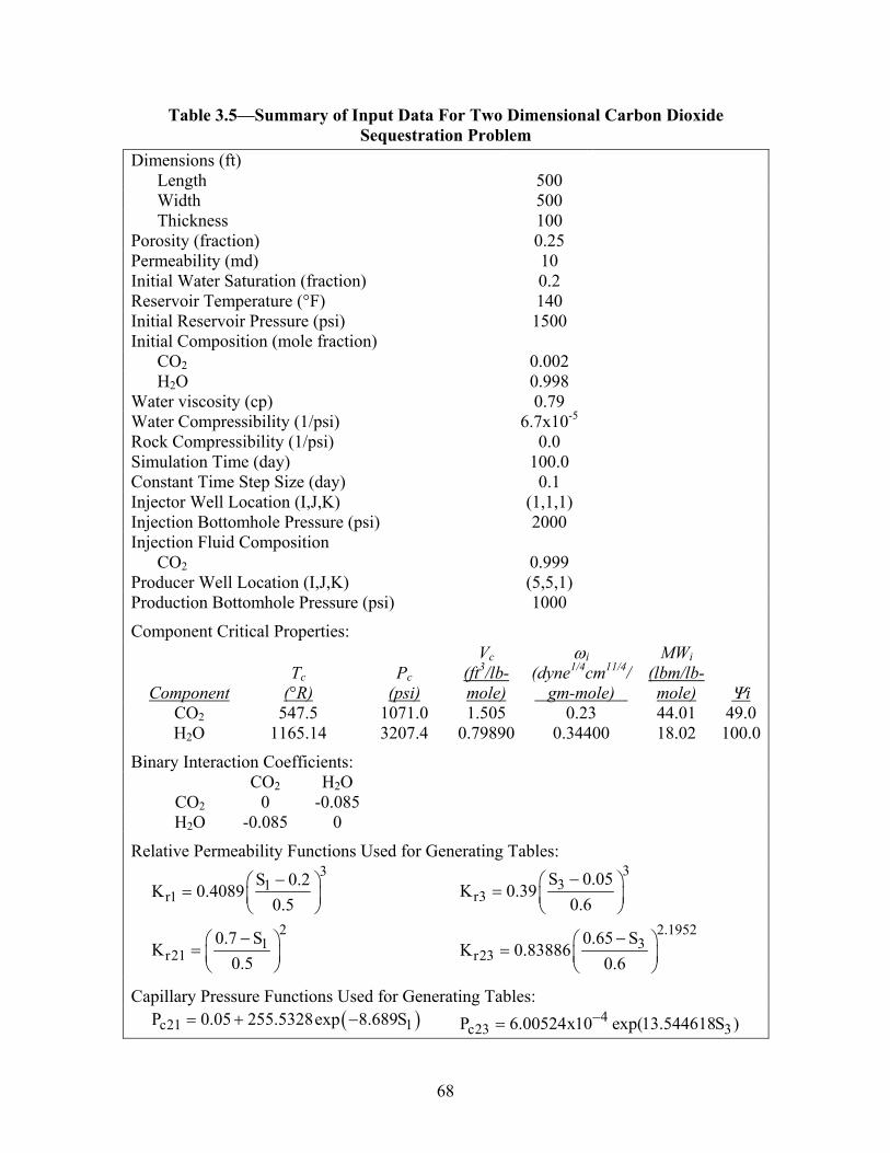
68
Table 3.5—Summary of Input Data For Two Dimensional Carbon Dioxide Sequestration Problem
Dimensions (ft) Length 500 Width 500 Thickness 100
Porosity (fraction) 0.25 Permeability (md) 10 Initial Water Saturation (fraction) 0.2 Reservoir Temperature (°F) 140 Initial Reservoir Pressure (psi) 1500 Initial Composition (mole fraction)
CO2 0.002 H2O 0.998
Water viscosity (cp) 0.79 Water Compressibility (1/psi) 6.7x10⁻⁵ Rock Compressibility (1/psi) 0.0 Simulation Time (day) 100.0 Constant Time Step Size (day) 0.1 Injector Well Location (I,J,K) (1,1,1) Injection Bottomhole Pressure (psi) 2000 Injection Fluid Composition
CO2 0.999 Producer Well Location (I,J,K) (5,5,1) Production Bottomhole Pressure (psi) 1000
Component Critical Properties:
Component Tc
(°R) Pc
(psi)
Vc (ft3/lb-mole)
ωi (dyne1/4cm11/4/ gm-mole)
MWi (lbm/lb-mole) Ψi
CO2 547.5 1071.0 1.505 0.23 44.01 49.0 H2O 1165.14 3207.4 0.79890 0.34400 18.02 100.0
Binary Interaction Coefficients: CO2 H2O CO2 0 -0.085 H2O -0.085 0
Relative Permeability Functions Used for Generating Tables: 3
1r1
21
r21
S 0.2K 0.4089
0.5
0.7 SK
0.5
− =
− =
33
r3
2.19523
r23
S 0.05K 0.39
0.6
0.65 SK 0.83886
0.6
− =
− =
Capillary Pressure Functions Used for Generating Tables: ( )c21 1P 0.05 255.5328exp 8.689S= + − 4
c23 3P 6.00524x10 exp(13.544618S )−=
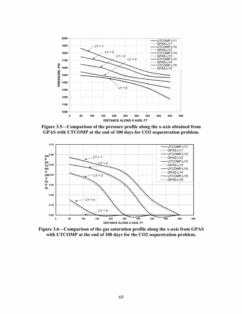
69
1000
1100
1200
1300
1400
1500
1600
1700
1800
1900
2000
0 50 100 150 200 250 300 350 400 450 500
DISTANCE ALONG X AXIS, FT
PRES
SUR
E, P
SI
UTCOMP-LY1GPAS-LY1UTCOMP-LY2GPAS-LY2UTCOMP-LY3GPAS-LY3UTCOMP-LY4GPAS-LY4UTCOMP-LY5GPAS-LY5
LY = 1
LY = 2LY = 3
LY = 4
LY = 5
Figure 3.5—Comparison of the pressure profile along the x-axis obtained from GPAS with UTCOMP at the end of 100 days for CO2 sequestration problem.
0.00
0.10
0.20
0.30
0.40
0.50
0.60
0.70
0 50 100 150 200 250 300 350 400 450 500
DISTANCE ALONG X AXIS, FT
GASSATURATION,VOL/VOL
UTCOMP-LY1GPAS-LY1UTCOMP-LY2GPAS-LY2UTCOMP-LY3GPAS-LY3UTCOMP-LY4GPAS-LY4UTCOMP-LY5GPAS-LY5
LY = 1
LY = 2
LY = 3
LY = 4
LY = 5
Figure 3.6—Comparison of the gas saturation profile along the x-axis from GPAS
with UTCOMP at the end of 100 days for the CO2 sequestration problem.
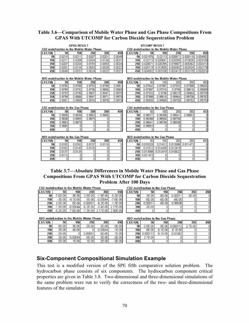
70
Table 3.6—Comparison of Mobile Water Phase and Gas Phase Compositions From GPAS With UTCOMP for Carbon Dioxide Sequestration Problem
Table 3.7—Absolute Differences in Mobile Water Phase and Gas Phase Compositions From GPAS With UTCOMP for Carbon Dioxide Sequestration
Problem After 100 Days
Six-Component Compositional Simulation Example This test is a modified version of the SPE fifth comparative solution problem. The hydrocarbon phase consists of six components. The hydrocarbon component critical properties are given in Table 3.8. Two-dimensional and three-dimensional simulations of the same problem were run to verify the correctness of the two- and three-dimensional features of the simulator.
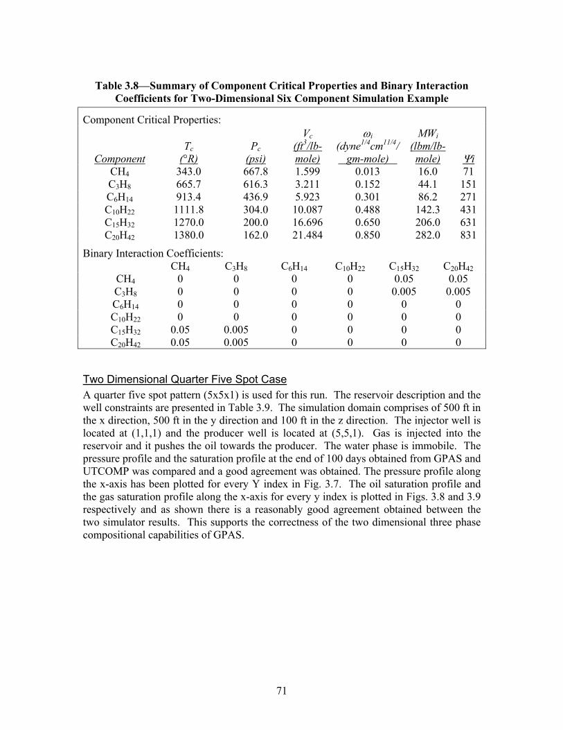
71
Table 3.8—Summary of Component Critical Properties and Binary Interaction
Coefficients for Two-Dimensional Six Component Simulation Example
Component Critical Properties:
Component Tc
(°R) Pc
(psi)
Vc (ft3/lb-mole)
ωi (dyne1/4cm11/4/ gm-mole)
MWi (lbm/lb-mole) Ψi
CH4 343.0 667.8 1.599 0.013 16.0 71 C3H8 665.7 616.3 3.211 0.152 44.1 151 C6H14 913.4 436.9 5.923 0.301 86.2 271 C10H22 1111.8 304.0 10.087 0.488 142.3 431 C15H32 1270.0 200.0 16.696 0.650 206.0 631 C20H42 1380.0 162.0 21.484 0.850 282.0 831
Binary Interaction Coefficients: CH4 C3H8 C6H14 C10H22 C15H32 C20H42 CH4 0 0 0 0 0.05 0.05 C3H8 0 0 0 0 0.005 0.005 C6H14 0 0 0 0 0 0 C10H22 0 0 0 0 0 0 C15H32 0.05 0.005 0 0 0 0 C20H42 0.05 0.005 0 0 0 0
Two Dimensional Quarter Five Spot Case A quarter five spot pattern (5x5x1) is used for this run. The reservoir description and the well constraints are presented in Table 3.9. The simulation domain comprises of 500 ft in the x direction, 500 ft in the y direction and 100 ft in the z direction. The injector well is located at (1,1,1) and the producer well is located at (5,5,1). Gas is injected into the reservoir and it pushes the oil towards the producer. The water phase is immobile. The pressure profile and the saturation profile at the end of 100 days obtained from GPAS and UTCOMP was compared and a good agreement was obtained. The pressure profile along the x-axis has been plotted for every Y index in Fig. 3.7. The oil saturation profile and the gas saturation profile along the x-axis for every y index is plotted in Figs. 3.8 and 3.9 respectively and as shown there is a reasonably good agreement obtained between the two simulator results. This supports the correctness of the two dimensional three phase compositional capabilities of GPAS.
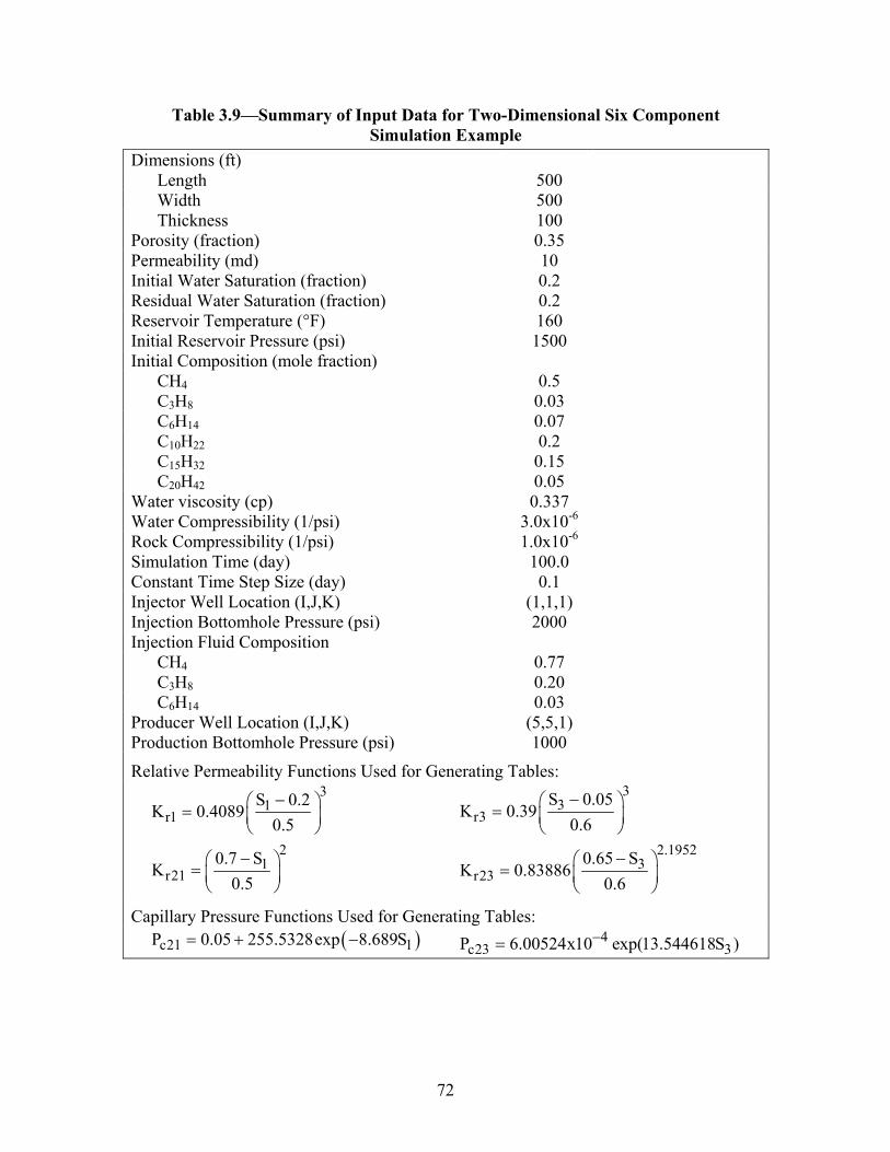
72
Table 3.9—Summary of Input Data for Two-Dimensional Six Component Simulation Example
Dimensions (ft) Length 500 Width 500 Thickness 100
Porosity (fraction) 0.35 Permeability (md) 10 Initial Water Saturation (fraction) 0.2 Residual Water Saturation (fraction) 0.2 Reservoir Temperature (°F) 160 Initial Reservoir Pressure (psi) 1500 Initial Composition (mole fraction)
CH4 0.5 C3H8 0.03 C6H14 0.07 C10H22 0.2 C15H32 0.15 C20H42 0.05
Water viscosity (cp) 0.337 Water Compressibility (1/psi) 3.0x10⁻⁶ Rock Compressibility (1/psi) 1.0x10⁻⁶ Simulation Time (day) 100.0 Constant Time Step Size (day) 0.1 Injector Well Location (I,J,K) (1,1,1) Injection Bottomhole Pressure (psi) 2000 Injection Fluid Composition
CH4 0.77 C3H8 0.20 C6H14 0.03
Producer Well Location (I,J,K) (5,5,1) Production Bottomhole Pressure (psi) 1000
Relative Permeability Functions Used for Generating Tables: 3
1r1
21
r21
S 0.2K 0.4089
0.5
0.7 SK
0.5
− =
− =
33
r3
2.19523
r23
S 0.05K 0.39
0.6
0.65 SK 0.83886
0.6
− =
− =
Capillary Pressure Functions Used for Generating Tables: ( )c21 1P 0.05 255.5328exp 8.689S= + − 4
c23 3P 6.00524x10 exp(13.544618S )−=
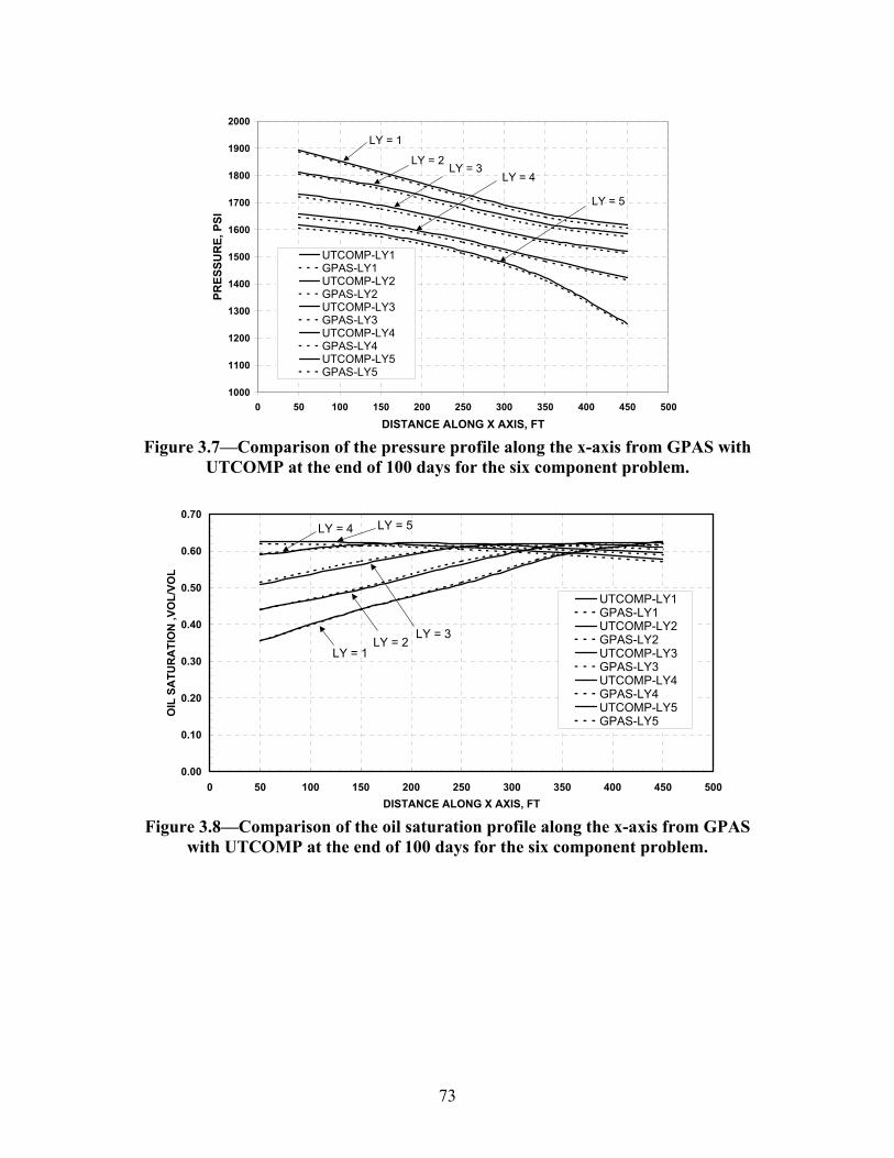
73
1000
1100
1200
1300
1400
1500
1600
1700
1800
1900
2000
0 50 100 150 200 250 300 350 400 450 500
DISTANCE ALONG X AXIS, FT
PRES
SUR
E, P
SI
UTCOMP-LY1GPAS-LY1UTCOMP-LY2GPAS-LY2UTCOMP-LY3GPAS-LY3UTCOMP-LY4GPAS-LY4UTCOMP-LY5GPAS-LY5
LY = 1
LY = 2LY = 3
LY = 4
LY = 5
Figure 3.7—Comparison of the pressure profile along the x-axis from GPAS with
UTCOMP at the end of 100 days for the six component problem.
0.00
0.10
0.20
0.30
0.40
0.50
0.60
0.70
0 50 100 150 200 250 300 350 400 450 500DISTANCE ALONG X AXIS, FT
OIL
SA
TUR
ATI
ON
,VO
L/VO
L
UTCOMP-LY1GPAS-LY1UTCOMP-LY2GPAS-LY2UTCOMP-LY3GPAS-LY3UTCOMP-LY4GPAS-LY4UTCOMP-LY5GPAS-LY5
LY = 1LY = 2
LY = 3
LY = 4 LY = 5
Figure 3.8—Comparison of the oil saturation profile along the x-axis from GPAS
with UTCOMP at the end of 100 days for the six component problem.
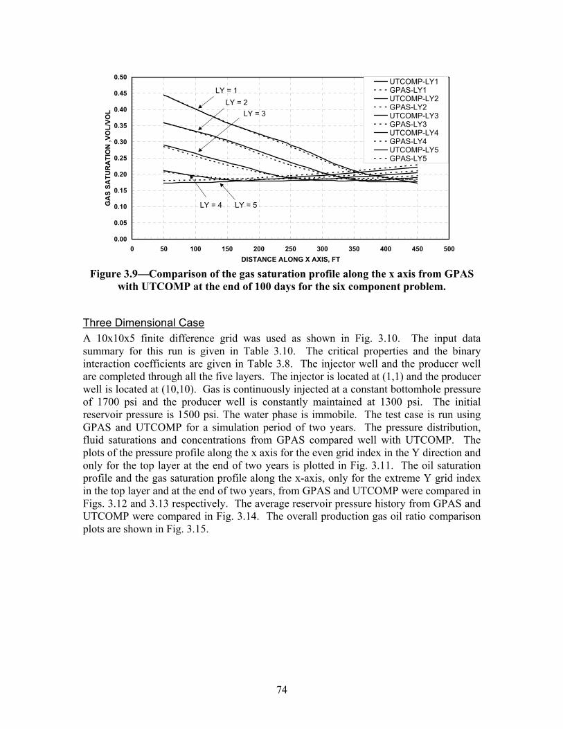
74
0.00
0.05
0.10
0.15
0.20
0.25
0.30
0.35
0.40
0.45
0.50
0 50 100 150 200 250 300 350 400 450 500DISTANCE ALONG X AXIS, FT
GA
S SA
TUR
ATI
ON
,VO
L/VO
L
UTCOMP-LY1GPAS-LY1UTCOMP-LY2GPAS-LY2UTCOMP-LY3GPAS-LY3UTCOMP-LY4GPAS-LY4UTCOMP-LY5GPAS-LY5
LY = 1LY = 2
LY = 3
LY = 4 LY = 5
Figure 3.9—Comparison of the gas saturation profile along the x axis from GPAS
with UTCOMP at the end of 100 days for the six component problem.
Three Dimensional Case A 10x10x5 finite difference grid was used as shown in Fig. 3.10. The input data summary for this run is given in Table 3.10. The critical properties and the binary interaction coefficients are given in Table 3.8. The injector well and the producer well are completed through all the five layers. The injector is located at (1,1) and the producer well is located at (10,10). Gas is continuously injected at a constant bottomhole pressure of 1700 psi and the producer well is constantly maintained at 1300 psi. The initial reservoir pressure is 1500 psi. The water phase is immobile. The test case is run using GPAS and UTCOMP for a simulation period of two years. The pressure distribution, fluid saturations and concentrations from GPAS compared well with UTCOMP. The plots of the pressure profile along the x axis for the even grid index in the Y direction and only for the top layer at the end of two years is plotted in Fig. 3.11. The oil saturation profile and the gas saturation profile along the x-axis, only for the extreme Y grid index in the top layer and at the end of two years, from GPAS and UTCOMP were compared in Figs. 3.12 and 3.13 respectively. The average reservoir pressure history from GPAS and UTCOMP were compared in Fig. 3.14. The overall production gas oil ratio comparison plots are shown in Fig. 3.15.
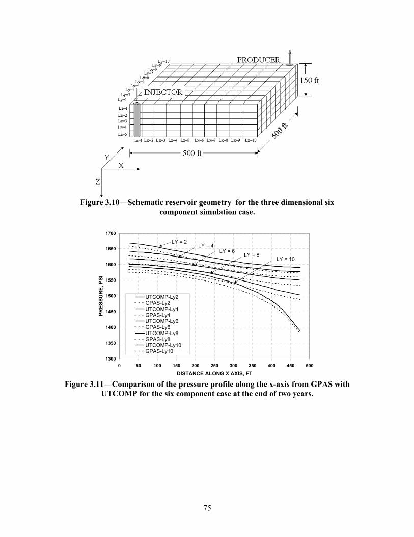
75
Figure 3.10—Schematic reservoir geometry for the three dimensional six
component simulation case.
1300
1350
1400
1450
1500
1550
1600
1650
1700
0 50 100 150 200 250 300 350 400 450 500
DISTANCE ALONG X AXIS, FT
PRES
SUR
E, P
SI
UTCOMP-Ly2GPAS-Ly2UTCOMP-Ly4GPAS-Ly4UTCOMP-Ly6GPAS-Ly6UTCOMP-Ly8GPAS-Ly8UTCOMP-Ly10GPAS-Ly10
LY = 2LY = 4
LY = 6LY = 8
LY = 10
Figure 3.11—Comparison of the pressure profile along the x-axis from GPAS with
UTCOMP for the six component case at the end of two years.
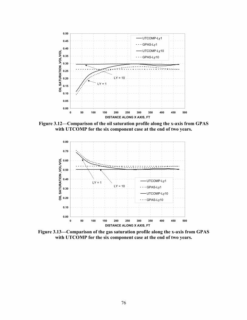
76
0.00
0.05
0.10
0.15
0.20
0.25
0.30
0.35
0.40
0.45
0.50
0 50 100 150 200 250 300 350 400 450 500
DISTANCE ALONG X AXIS, FT
OIL
SA
TUR
ATI
ON
,VO
L/VO
L
UTCOMP-Ly1
GPAS-Ly1
UTCOMP-Ly10
GPAS-Ly10
LY = 1
LY = 10
Figure 3.12—Comparison of the oil saturation profile along the x-axis from GPAS
with UTCOMP for the six component case at the end of two years.
0.00
0.10
0.20
0.30
0.40
0.50
0.60
0.70
0.80
0 50 100 150 200 250 300 350 400 450 500
DISTANCE ALONG X AXIS, FT
OIL
SA
TUR
ATI
ON
,VO
L/VO
L
UTCOMP-Ly1
GPAS-Ly1
UTCOMP-Ly10
GPAS-Ly10
LY = 1LY = 10
Figure 3.13—Comparison of the gas saturation profile along the x-axis from GPAS
with UTCOMP for the six component case at the end of two years.
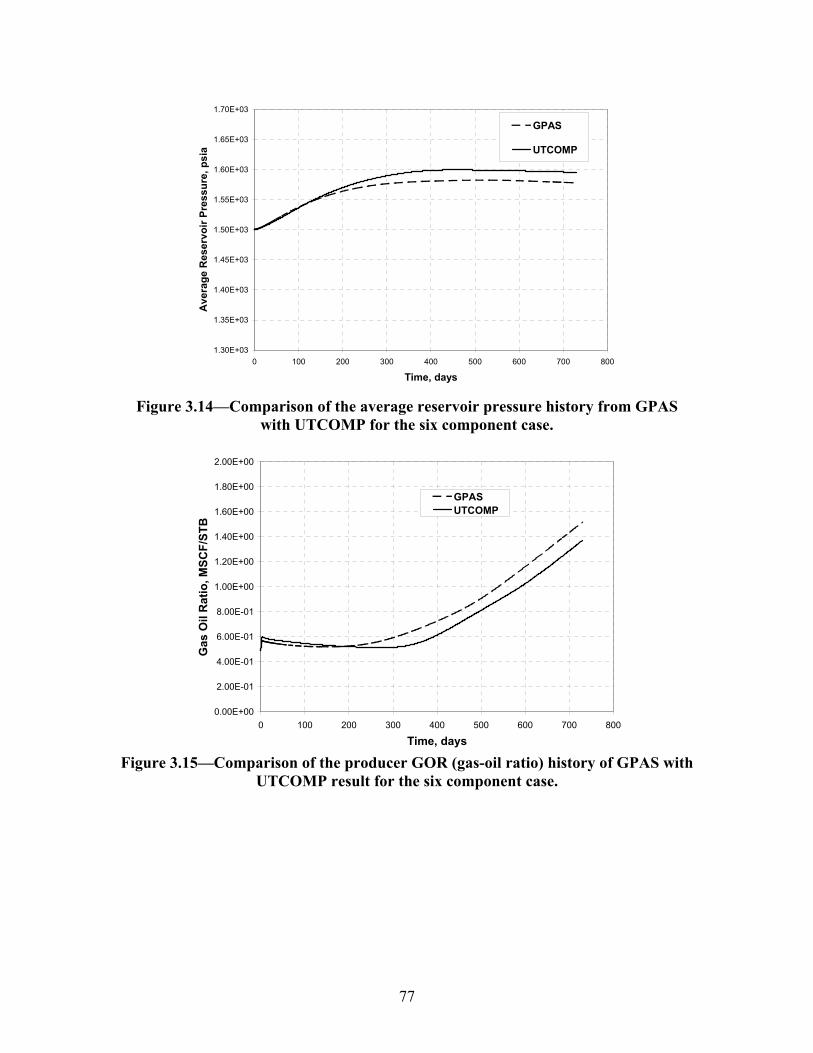
77
1.30E+03
1.35E+03
1.40E+03
1.45E+03
1.50E+03
1.55E+03
1.60E+03
1.65E+03
1.70E+03
0 100 200 300 400 500 600 700 800
Time, days
Ave
rage
Res
ervo
ir Pr
essu
re, p
sia
GPAS
UTCOMP
Figure 3.14—Comparison of the average reservoir pressure history from GPAS
with UTCOMP for the six component case.
0.00E+00
2.00E-01
4.00E-01
6.00E-01
8.00E-01
1.00E+00
1.20E+00
1.40E+00
1.60E+00
1.80E+00
2.00E+00
0 100 200 300 400 500 600 700 800
Time, days
Gas
Oil
Rat
io, M
SCF/
STB
GPASUTCOMP
Figure 3.15—Comparison of the producer GOR (gas-oil ratio) history of GPAS with
UTCOMP result for the six component case.
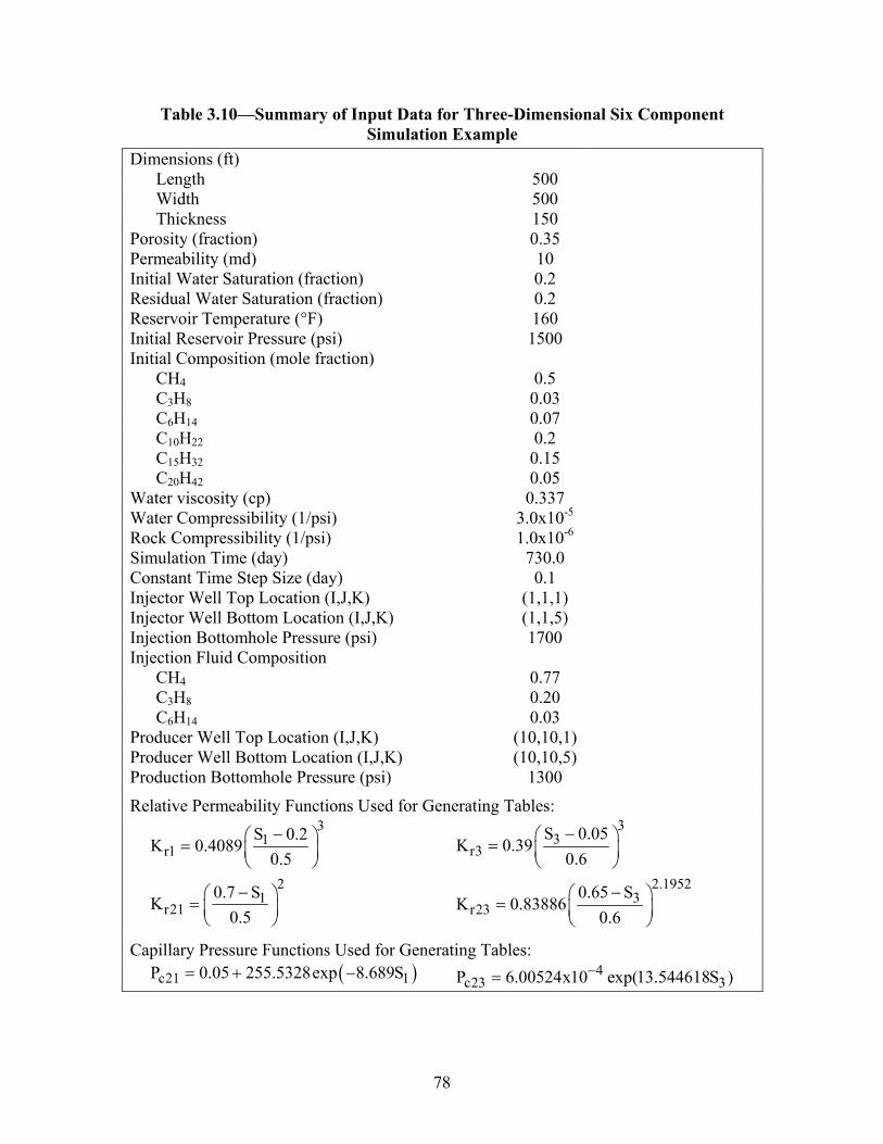
78
Table 3.10—Summary of Input Data for Three-Dimensional Six Component Simulation Example
Dimensions (ft) Length 500 Width 500 Thickness 150
Porosity (fraction) 0.35 Permeability (md) 10 Initial Water Saturation (fraction) 0.2 Residual Water Saturation (fraction) 0.2 Reservoir Temperature (°F) 160 Initial Reservoir Pressure (psi) 1500 Initial Composition (mole fraction)
CH4 0.5 C3H8 0.03 C6H14 0.07 C10H22 0.2 C15H32 0.15 C20H42 0.05
Water viscosity (cp) 0.337 Water Compressibility (1/psi) 3.0x10⁻⁵ Rock Compressibility (1/psi) 1.0x10⁻⁶ Simulation Time (day) 730.0 Constant Time Step Size (day) 0.1 Injector Well Top Location (I,J,K) (1,1,1) Injector Well Bottom Location (I,J,K) (1,1,5) Injection Bottomhole Pressure (psi) 1700 Injection Fluid Composition
CH4 0.77 C3H8 0.20 C6H14 0.03
Producer Well Top Location (I,J,K) (10,10,1) Producer Well Bottom Location (I,J,K) (10,10,5) Production Bottomhole Pressure (psi) 1300
Relative Permeability Functions Used for Generating Tables: 3
1r1
21
r21
S 0.2K 0.4089
0.5
0.7 SK
0.5
− =
− =
33
r3
2.19523
r23
S 0.05K 0.39
0.6
0.65 SK 0.83886
0.6
− =
− =
Capillary Pressure Functions Used for Generating Tables: ( )c21 1P 0.05 255.5328exp 8.689S= + − 4
c23 3P 6.00524x10 exp(13.544618S )−=
79
Chemical Module Tests—Explicit Formulation The chemical module of the GPAS simulator has been validated by comparing results with analytical solutions for one dimensional aqueous species transport and with the results of The University of Texas Chemical Simulator (UTCHEM). In this section, we present a comparison with UTCHEM that has been validated by comparisons with analytical solutions, laboratory surfactant floods and a variety of laboratory and field results.
2-D Surfactant/Polymer Simulation, Case 1 A two-dimensional test case was setup to model surfactant-polymer slug injection in a quarter of five-spot well pattern. The input data used is summarized in Table 3.11. The reservoir is 480 ft in each direction modeled by a 15x15 grid. The rock properties and relative permeability input are set for typical water wet conditions. The polymer viscosity parameters resulted in viscosity of about 12 cp at the maximum polymer concentration used in the simulation (0.05 wt%). The oil phase was modeled using single component n-decane and the resulting phase properties (as computed by the EOS model) were used in UTCHEM. It must be noted that UTCHEM uses constant fluid compressibility and density whereas these are updated for each timestep of the EOS model based on the composition and pressure. For the sake of comparison, model parameters are set to allow not much variation in fluid properties over the range of changes encountered during the run. The results are compared with UTCHEM output in Figs. 3.16 through 3.25. The surfactant, tracer and polymer concentration histories agree well (Figs. 3.16, 3.17 and 3.18). Figures 3.19 and 3.20 show the polymer concentration profiles at 0.5 PV injected, which agree well. The surfactant concentration profiles at the same time are shown in Figs. 3.21 and 3.22. The UTCHEM profile shows a slightly larger spread than GPAS. The oil saturation profiles (Fig. 3.23 and 3.24) show the effect of the chemical slug. The mobilized oil is pushed ahead of the surfactant forming an oil bank and leaving very little oil in the swept region of the reservoir. UTCHEM oil saturations are slightly lower in the swept region because it accounts for additional oil removal by solubilization. Figure 3.25 shows the comparison of oil production rates and cumulative oil recovery. The breakthrough times for the oil bank and the oil production rates are in satisfactory agreement. The cumulative oil recovery using UTCHEM is 7% higher than for GPAS due to the additional solubilized oil not accounted for in GPAS.

80
Table 3.11—Input parameters used for Case 1 Property Value
Reservoir Size 480ft x 480ft x 50ft Reservoir Gridblock Size 32ft x 32ft x 50ft Number of Gridblocks 15 x 15 x 1 Matrix Permeability 540 md Matrix Porosity 0.136 Initial Water Saturation 0.75 Initial Pressure 200 psi Water Viscosity 1 cp Oil Viscosity 2.6 cp Oil Specific Gravity 0.3858 psi/ft Oil Compressibility 3x10⁻⁶ 1/psi Polymer Viscosity Parameters 81, 2700, 2500 Surfactant Properties
Heights of Binodal Curve 0.07, 0.04 vol. fraction Salinity Limits 0.177, 0.25 meq/ml CMC 0.0001 vol. fraction Adsorption Parameters 1.5, 0.5, 1000 IFT Correlation Parameters (a,c) 9, 0.2
Relative Permeability Model Residual Saturations at Low Trapping Number 0.14, 0.25, 0.0 Residual Saturations at High Trapping Number 0.0, 0.0, 0.0 Endpoints at Low Trapping Number 0.106, 0.8, 0.0 Endpoints at High Trapping Number 1.0, 1.0, 1.0 Exponents at Low Trapping Number 2.1, 1.7, 0.0 Exponents at High Trapping Number 0.48, 1.5, 0.0 Trapping Number Parameters 364, 59074, 364
1.0, 1.0, 1.0 Injection Rate 3000 ft3/day Production Constraint (BHP) 200.0 psi Chemical Slug Size 0.2 PV Chemical Slug Composition 0.17 meq/ml salt, 0.05 vol.
fraction, surfactant, 0.05 wt % polymer, water, tracer
Chase Fluid Composition 0.17 meq/ml salt, 0.05 wt % polymer, water
Simulation Time 2 PV
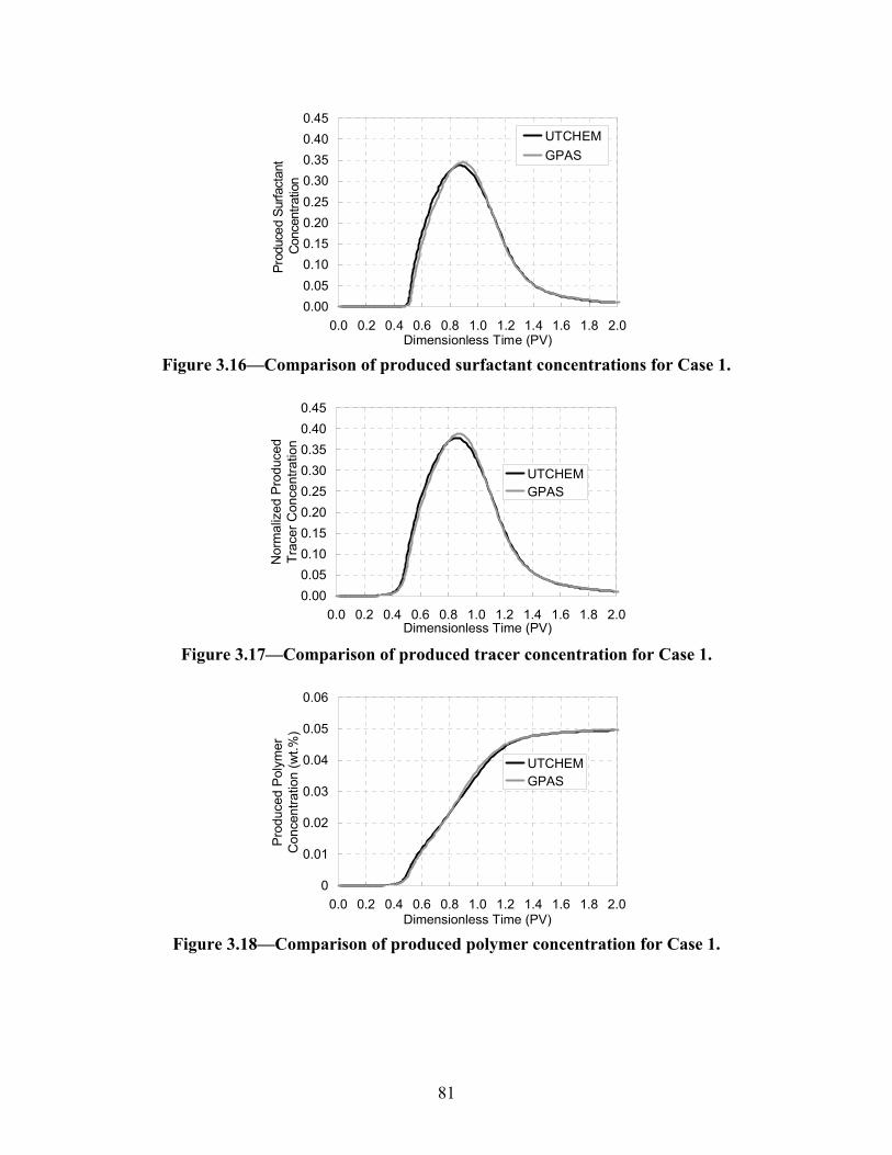
81
0.000.050.100.150.200.250.300.350.400.45
0.0 0.2 0.4 0.6 0.8 1.0 1.2 1.4 1.6 1.8 2.0Dimensionless Time (PV)
Prod
uced
Sur
fact
ant
Conc
entra
tion
UTCHEMGPAS
Figure 3.16—Comparison of produced surfactant concentrations for Case 1.
0.000.050.100.150.200.250.300.350.400.45
0.0 0.2 0.4 0.6 0.8 1.0 1.2 1.4 1.6 1.8 2.0Dimensionless Time (PV)
Nor
mal
ized
Pro
duce
dTr
acer
Con
cent
ratio
n
UTCHEMGPAS
Figure 3.17—Comparison of produced tracer concentration for Case 1.
0
0.01
0.02
0.03
0.04
0.05
0.06
0.0 0.2 0.4 0.6 0.8 1.0 1.2 1.4 1.6 1.8 2.0Dimensionless Time (PV)
Pro
duce
d P
olym
er
Con
cent
ratio
n (w
t.%)
UTCHEMGPAS
Figure 3.18—Comparison of produced polymer concentration for Case 1.
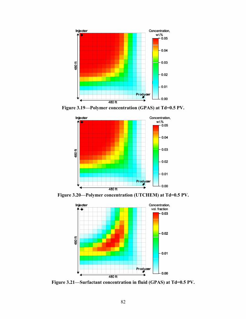
82
480 ft
480
ft
Concentration,wt.%
Injector
Producer
0.05
0.04
0.03
0.02
0.01
0.00480 ft480 ft
480
ft48
0 ft
Concentration,wt.%
Injector
Producer
0.05
0.04
0.03
0.02
0.01
0.00
Figure 3.19—Polymer concentration (GPAS) at Td=0.5 PV.
480 ft
480
ft
Concentration,wt.%
Injector
Producer
0.05
0.04
0.03
0.02
0.01
0.00480 ft480 ft
480
ft48
0 ft
Concentration,wt.%
Injector
Producer
0.05
0.04
0.03
0.02
0.01
0.00
Figure 3.20—Polymer concentration (UTCHEM) at Td=0.5 PV.
480 ft
480
ft
Concentration,vol. fraction
Injector
Producer
0.03
0.02
0.01
0.00480 ft480 ft
480
ft48
0 ft
Concentration,vol. fraction
Injector
Producer
0.03
0.02
0.01
0.00
0.03
0.02
0.01
0.00
Figure 3.21—Surfactant concentration in fluid (GPAS) at Td=0.5 PV.
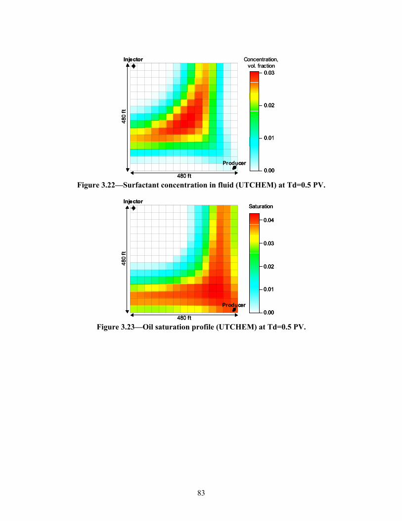
83
480 ft
480
ft
Concentration,vol. fraction
Injector
Producer
0.03
0.02
0.01
0.00480 ft480 ft
480
ft48
0 ft
Concentration,vol. fraction
Injector
Producer
0.03
0.02
0.01
0.00
0.03
0.02
0.01
0.00
Figure 3.22—Surfactant concentration in fluid (UTCHEM) at Td=0.5 PV.
480 ft
480
ft
Injector
Producer
Saturation
0.04
0.03
0.02
0.01
0.00480 ft480 ft
480
ft48
0 ft
Injector
Producer
Saturation
0.04
0.03
0.02
0.01
0.00
Saturation
0.04
0.03
0.02
0.01
0.00
Figure 3.23—Oil saturation profile (UTCHEM) at Td=0.5 PV.
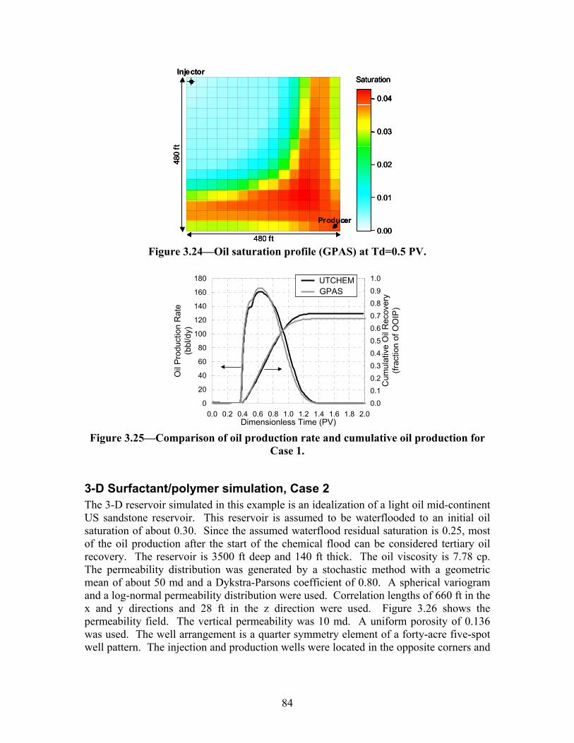
84
480 ft
480
ft
Injector
Producer
Saturation
0.04
0.03
0.02
0.01
0.00480 ft480 ft
480
ft48
0 ft
Injector
Producer
Saturation
0.04
0.03
0.02
0.01
0.00
Saturation
0.04
0.03
0.02
0.01
0.00
Figure 3.24—Oil saturation profile (GPAS) at Td=0.5 PV.
0
20
40
60
80
100
120
140
160
180
0.0 0.2 0.4 0.6 0.8 1.0 1.2 1.4 1.6 1.8 2.0Dimensionless Time (PV)
Oil
Pro
duct
ion
Rat
e (b
bl/d
y)
0.0
0.1
0.2
0.3
0.4
0.5
0.6
0.7
0.8
0.9
1.0
Cum
ulat
ive
Oil
Rec
over
y (fr
actio
n of
OO
IP)
UTCHEMGPAS
Figure 3.25—Comparison of oil production rate and cumulative oil production for
Case 1.
3-D Surfactant/polymer simulation, Case 2 The 3-D reservoir simulated in this example is an idealization of a light oil mid-continent US sandstone reservoir. This reservoir is assumed to be waterflooded to an initial oil saturation of about 0.30. Since the assumed waterflood residual saturation is 0.25, most of the oil production after the start of the chemical flood can be considered tertiary oil recovery. The reservoir is 3500 ft deep and 140 ft thick. The oil viscosity is 7.78 cp. The permeability distribution was generated by a stochastic method with a geometric mean of about 50 md and a Dykstra-Parsons coefficient of 0.80. A spherical variogram and a log-normal permeability distribution were used. Correlation lengths of 660 ft in the x and y directions and 28 ft in the z direction were used. Figure 3.26 shows the permeability field. The vertical permeability was 10 md. A uniform porosity of 0.136 was used. The well arrangement is a quarter symmetry element of a forty-acre five-spot well pattern. The injection and production wells were located in the opposite corners and
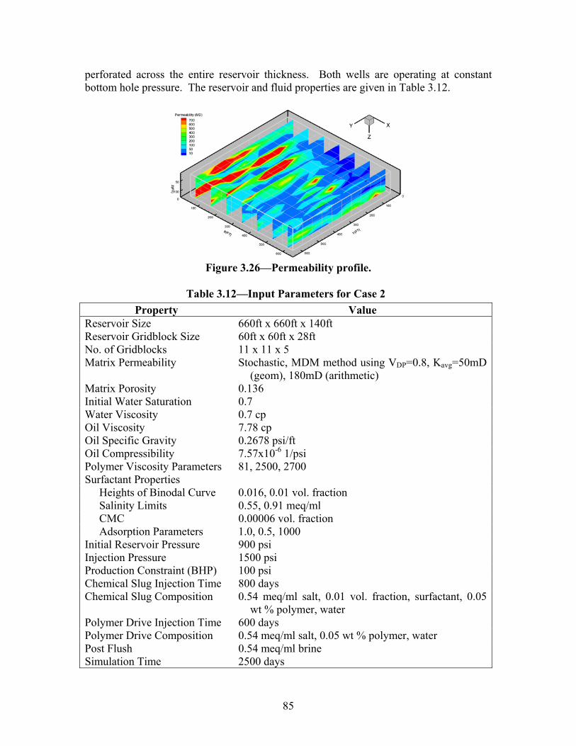
85
perforated across the entire reservoir thickness. Both wells are operating at constant bottom hole pressure. The reservoir and fluid properties are given in Table 3.12.
Figure 3.26—Permeability profile.
Table 3.12—Input Parameters for Case 2
Property Value Reservoir Size 660ft x 660ft x 140ft Reservoir Gridblock Size 60ft x 60ft x 28ft No. of Gridblocks 11 x 11 x 5 Matrix Permeability Stochastic, MDM method using VDP=0.8, Kavg=50mD
(geom), 180mD (arithmetic) Matrix Porosity 0.136 Initial Water Saturation 0.7 Water Viscosity 0.7 cp Oil Viscosity 7.78 cp Oil Specific Gravity 0.2678 psi/ft Oil Compressibility 7.57x10⁻⁶ 1/psi Polymer Viscosity Parameters 81, 2500, 2700 Surfactant Properties
Heights of Binodal Curve 0.016, 0.01 vol. fraction Salinity Limits 0.55, 0.91 meq/ml CMC 0.00006 vol. fraction Adsorption Parameters 1.0, 0.5, 1000
Initial Reservoir Pressure 900 psi Injection Pressure 1500 psi Production Constraint (BHP) 100 psi Chemical Slug Injection Time 800 days Chemical Slug Composition 0.54 meq/ml salt, 0.01 vol. fraction, surfactant, 0.05
wt % polymer, water Polymer Drive Injection Time 600 days Polymer Drive Composition 0.54 meq/ml salt, 0.05 wt % polymer, water Post Flush 0.54 meq/ml brine Simulation Time 2500 days
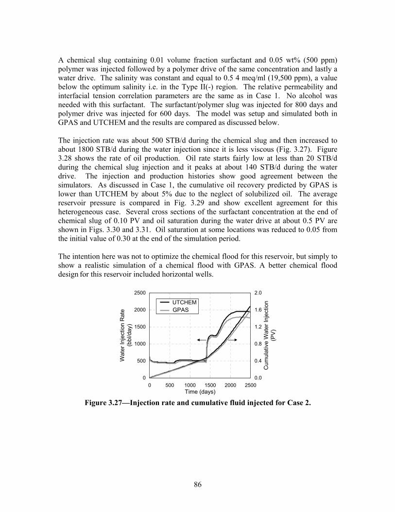
86
A chemical slug containing 0.01 volume fraction surfactant and 0.05 wt% (500 ppm) polymer was injected followed by a polymer drive of the same concentration and lastly a water drive. The salinity was constant and equal to 0.5 4 meq/ml (19,500 ppm), a value below the optimum salinity i.e. in the Type II(-) region. The relative permeability and interfacial tension correlation parameters are the same as in Case 1. No alcohol was needed with this surfactant. The surfactant/polymer slug was injected for 800 days and polymer drive was injected for 600 days. The model was setup and simulated both in GPAS and UTCHEM and the results are compared as discussed below. The injection rate was about 500 STB/d during the chemical slug and then increased to about 1800 STB/d during the water injection since it is less viscous (Fig. 3.27). Figure 3.28 shows the rate of oil production. Oil rate starts fairly low at less than 20 STB/d during the chemical slug injection and it peaks at about 140 STB/d during the water drive. The injection and production histories show good agreement between the simulators. As discussed in Case 1, the cumulative oil recovery predicted by GPAS is lower than UTCHEM by about 5% due to the neglect of solubilized oil. The average reservoir pressure is compared in Fig. 3.29 and show excellent agreement for this heterogeneous case. Several cross sections of the surfactant concentration at the end of chemical slug of 0.10 PV and oil saturation during the water drive at about 0.5 PV are shown in Figs. 3.30 and 3.31. Oil saturation at some locations was reduced to 0.05 from the initial value of 0.30 at the end of the simulation period. The intention here was not to optimize the chemical flood for this reservoir, but simply to show a realistic simulation of a chemical flood with GPAS. A better chemical flood design for this reservoir included horizontal wells.
0
500
1000
1500
2000
2500
0 500 1000 1500 2000 2500Time (days)
Wat
er In
ject
ion
Rat
e (b
bl/d
ay)
0.0
0.4
0.8
1.2
1.6
2.0
Cum
ulat
ive
Wat
er In
ject
ion
(PV)
UTCHEMGPAS
Figure 3.27—Injection rate and cumulative fluid injected for Case 2.
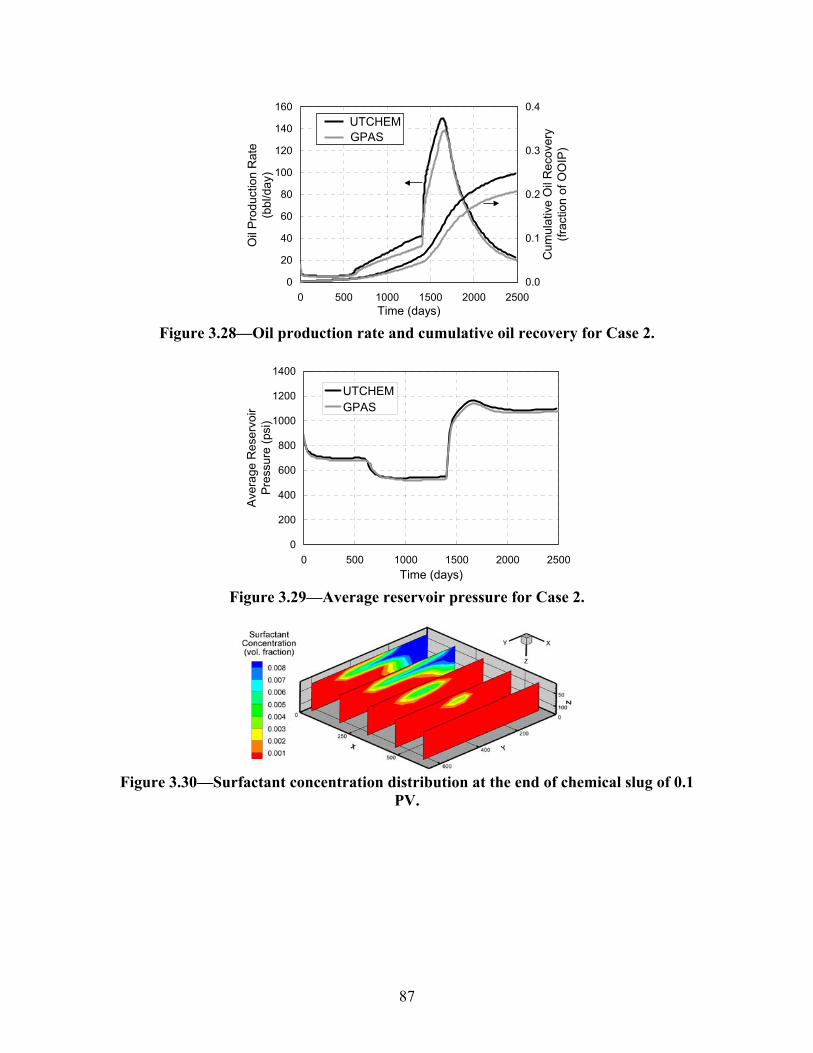
87
0
20
40
60
80
100
120
140
160
0 500 1000 1500 2000 2500Time (days)
Oil
Pro
duct
ion
Rat
e (b
bl/d
ay)
0.0
0.1
0.2
0.3
0.4
Cum
ulat
ive
Oil
Rec
over
y (fr
actio
n of
OO
IP)
UTCHEMGPAS
Figure 3.28—Oil production rate and cumulative oil recovery for Case 2.
0
200
400
600
800
1000
1200
1400
0 500 1000 1500 2000 2500Time (days)
Ave
rage
Res
ervo
irPr
essu
re (p
si)
UTCHEMGPAS
Figure 3.29—Average reservoir pressure for Case 2.
Figure 3.30—Surfactant concentration distribution at the end of chemical slug of 0.1
PV.
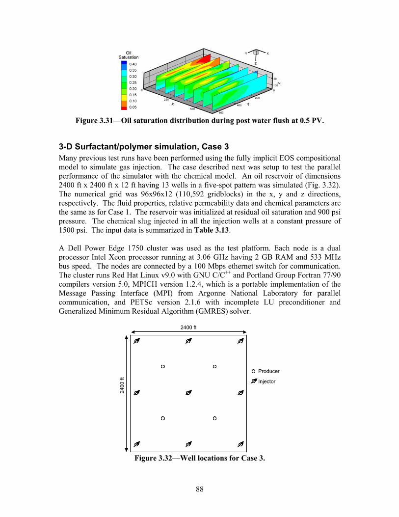
88
Figure 3.31—Oil saturation distribution during post water flush at 0.5 PV.
3-D Surfactant/polymer simulation, Case 3 Many previous test runs have been performed using the fully implicit EOS compositional model to simulate gas injection. The case described next was setup to test the parallel performance of the simulator with the chemical model. An oil reservoir of dimensions 2400 ft x 2400 ft x 12 ft having 13 wells in a five-spot pattern was simulated (Fig. 3.32). The numerical grid was 96x96x12 (110,592 gridblocks) in the x, y and z directions, respectively. The fluid properties, relative permeability data and chemical parameters are the same as for Case 1. The reservoir was initialized at residual oil saturation and 900 psi pressure. The chemical slug injected in all the injection wells at a constant pressure of 1500 psi. The input data is summarized in Table 3.13. A Dell Power Edge 1750 cluster was used as the test platform. Each node is a dual processor Intel Xeon processor running at 3.06 GHz having 2 GB RAM and 533 MHz bus speed. The nodes are connected by a 100 Mbps ethernet switch for communication. The cluster runs Red Hat Linux v9.0 with GNU C/C++ and Portland Group Fortran 77/90 compilers version 5.0, MPICH version 1.2.4, which is a portable implementation of the Message Passing Interface (MPI) from Argonne National Laboratory for parallel communication, and PETSc version 2.1.6 with incomplete LU preconditioner and Generalized Minimum Residual Algorithm (GMRES) solver.
2400
ft
2400 ft
Injector
Producer
Figure 3.32—Well locations for Case 3.
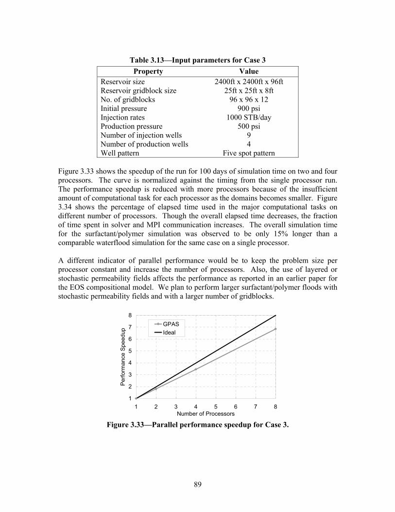
89
Table 3.13—Input parameters for Case 3 Property Value
Reservoir size 2400ft x 2400ft x 96ft Reservoir gridblock size 25ft x 25ft x 8ft No. of gridblocks 96 x 96 x 12 Initial pressure 900 psi Injection rates 1000 STB/day Production pressure 500 psi Number of injection wells 9 Number of production wells 4 Well pattern Five spot pattern
Figure 3.33 shows the speedup of the run for 100 days of simulation time on two and four processors. The curve is normalized against the timing from the single processor run. The performance speedup is reduced with more processors because of the insufficient amount of computational task for each processor as the domains becomes smaller. Figure 3.34 shows the percentage of elapsed time used in the major computational tasks on different number of processors. Though the overall elapsed time decreases, the fraction of time spent in solver and MPI communication increases. The overall simulation time for the surfactant/polymer simulation was observed to be only 15% longer than a comparable waterflood simulation for the same case on a single processor. A different indicator of parallel performance would be to keep the problem size per processor constant and increase the number of processors. Also, the use of layered or stochastic permeability fields affects the performance as reported in an earlier paper for the EOS compositional model. We plan to perform larger surfactant/polymer floods with stochastic permeability fields and with a larger number of gridblocks.
1
2
3
4
5
6
7
8
1 2 3 4 5 6 7 8Number of Processors
Perfo
rman
ce S
peed
up
GPASIdeal
Figure 3.33—Parallel performance speedup for Case 3.

90
0
10
20
30
40
50
60
70
80
1 2 4 8Number of Processors
Per
cent
age
ofTo
tal E
laps
ed T
ime
SOLVER JACOBIAN MPI
Figure 3.34—Comparison of time spent in solver, Jacobian and MPI communication
for Case 3.
Chemical Module Tests—Fully Implicit Formulation
1-D Surfactant/Polymer Flood The first validation test was based on a 1-D surfactant/polymer flood simulation with 100 gridblocks in the x direction. The purpose of this simulation was to compare the formulation and the implementation of the fully implicit chemical module against both UTCHEM and the explicit method of GPAS. The simulation domain consisted of 400 ft in the x direction, 1 ft in the y direction and 1 ft in the z direction. An injector was located at the grid index (1,1,1) operating at a constant rate of 0.5 STB/d and a producer located at the (100,1,1) operating at a constant bottomhole pressure of 20 psi. Surfactant slug contained 1% surfactant and 500 ppm polymer with a salt concentration of about 0.17 meq/ml. The slug was injected for about 11.4 days followed by a polymer drive of about 500 ppm concentration. A conservative tracer was also injected during the chemical slug. The results are favorably compared with those of UTCHEM and GPAS explicit formulation in Figs. 3.35 through 3.40.
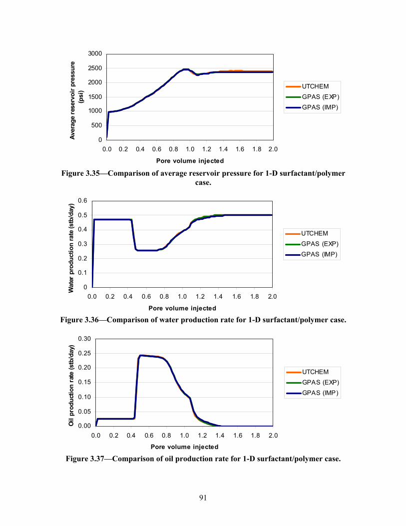
91
0
500
1000
1500
2000
2500
3000
0.0 0.2 0.4 0.6 0.8 1.0 1.2 1.4 1.6 1.8 2.0
Pore volume injected
Aver
age
rese
rvoi
r pre
ssur
e (p
si) UTCHEM
GPAS (EXP)GPAS (IMP)
Figure 3.35—Comparison of average reservoir pressure for 1-D surfactant/polymer
case.
0
0.1
0.2
0.3
0.4
0.5
0.6
0.0 0.2 0.4 0.6 0.8 1.0 1.2 1.4 1.6 1.8 2.0
Pore volume injected
Wat
er p
rodu
ctio
n ra
te (s
tb/d
ay)
UTCHEMGPAS (EXP)GPAS (IMP)
Figure 3.36—Comparison of water production rate for 1-D surfactant/polymer case.
0.00
0.05
0.10
0.15
0.20
0.25
0.30
0.0 0.2 0.4 0.6 0.8 1.0 1.2 1.4 1.6 1.8 2.0
Pore volume injected
Oil
prod
uctio
n ra
te (s
tb/d
ay)
UTCHEMGPAS (EXP)GPAS (IMP)
Figure 3.37—Comparison of oil production rate for 1-D surfactant/polymer case.
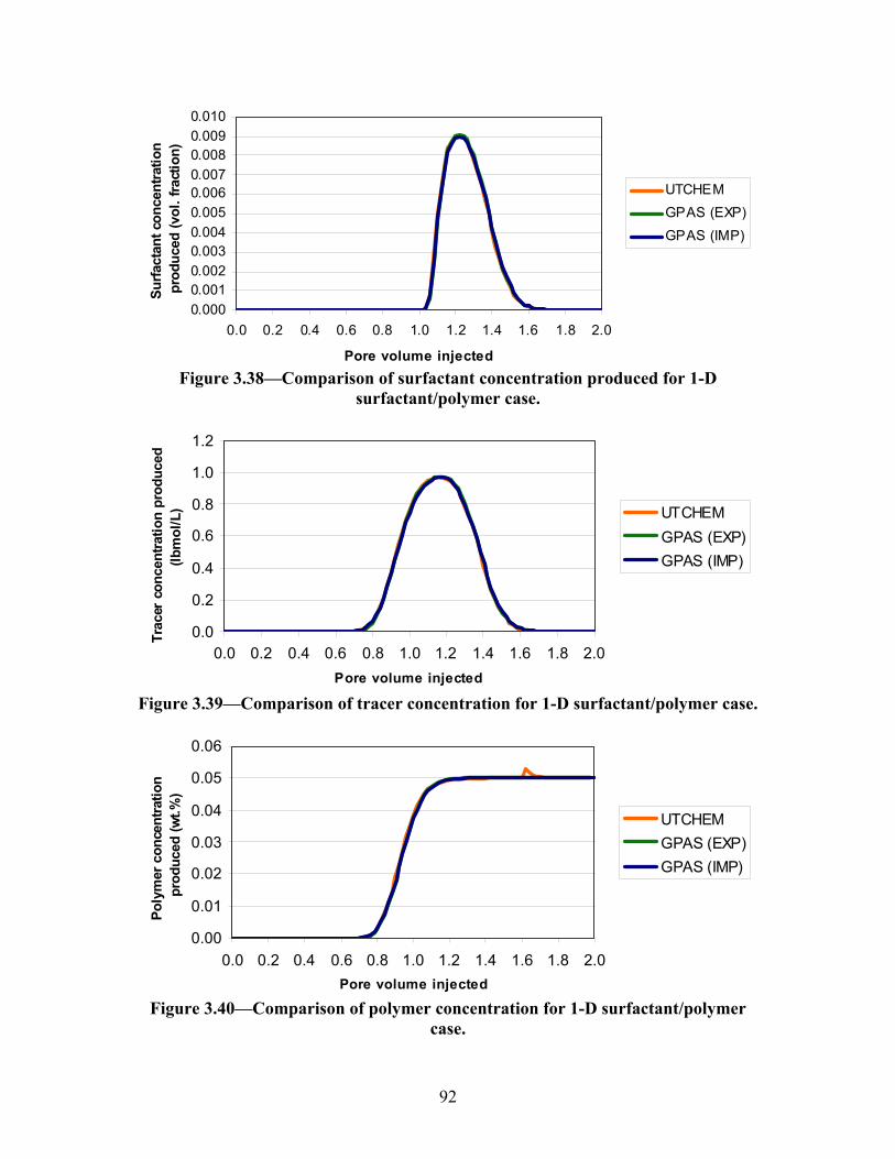
92
0.0000.0010.0020.0030.0040.0050.0060.0070.0080.0090.010
0.0 0.2 0.4 0.6 0.8 1.0 1.2 1.4 1.6 1.8 2.0
Pore volume injected
Surfa
ctan
t con
cent
ratio
n pr
oduc
ed (v
ol. f
ract
ion)
UTCHEMGPAS (EXP)GPAS (IMP)
Figure 3.38—Comparison of surfactant concentration produced for 1-D
surfactant/polymer case.
0.0
0.2
0.4
0.6
0.8
1.0
1.2
0.0 0.2 0.4 0.6 0.8 1.0 1.2 1.4 1.6 1.8 2.0Pore volume injected
Trac
er c
once
ntra
tion
prod
uced
(lb
mol
/L) UTCHEM
GPAS (EXP)GPAS (IMP)
Figure 3.39—Comparison of tracer concentration for 1-D surfactant/polymer case.
0.00
0.01
0.02
0.03
0.04
0.05
0.06
0.0 0.2 0.4 0.6 0.8 1.0 1.2 1.4 1.6 1.8 2.0Pore volume injected
Poly
mer
con
cent
ratio
n pr
oduc
ed (w
t.%)
UTCHEMGPAS (EXP)GPAS (IMP)
Figure 3.40—Comparison of polymer concentration for 1-D surfactant/polymer
case.
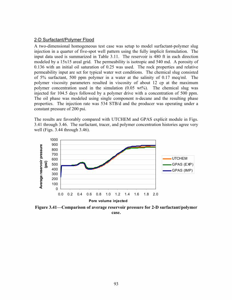
93
2-D Surfactant/Polymer Flood A two-dimensional homogeneous test case was setup to model surfactant-polymer slug injection in a quarter of five-spot well pattern using the fully implicit formulation. The input data used is summarized in Table 3.11. The reservoir is 480 ft in each direction modeled by a 15x15 areal grid. The permeability is isotropic and 540 md. A porosity of 0.136 with an initial oil saturation of 0.25 was used. The rock properties and relative permeability input are set for typical water wet conditions. The chemical slug consisted of 5% surfactant, 500 ppm polymer in a water at the salinity of 0.17 meq/ml. The polymer viscosity parameters resulted in viscosity of about 12 cp at the maximum polymer concentration used in the simulation (0.05 wt%). The chemical slug was injected for 104.5 days followed by a polymer drive with a concentration of 500 ppm. The oil phase was modeled using single component n-decane and the resulting phase properties. The injection rate was 534 STB/d and the producer was operating under a constant pressure of 200 psi. The results are favorably compared with UTCHEM and GPAS explicit module in Figs. 3.41 through 3.46. The surfactant, tracer, and polymer concentration histories agree very well (Figs. 3.44 through 3.46).
0100200300400500600700800900
1000
0.0 0.2 0.4 0.6 0.8 1.0 1.2 1.4 1.6 1.8 2.0
Pore volume injected
Aver
age
rese
rvoi
r pre
ssur
e (p
si) UTCHEM
GPAS (EXP)GPAS (IMP)
Figure 3.41—Comparison of average reservoir pressure for 2-D surfactant/polymer
case.
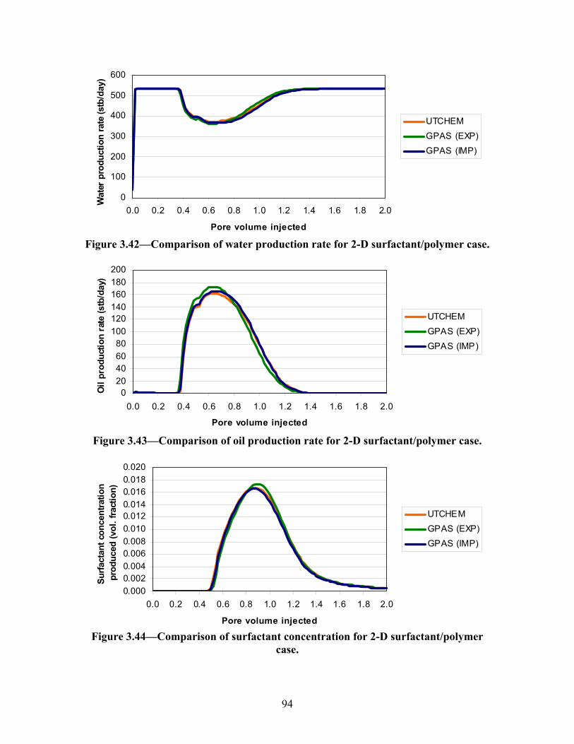
94
0
100
200
300
400
500
600
0.0 0.2 0.4 0.6 0.8 1.0 1.2 1.4 1.6 1.8 2.0
Pore volume injected
Wat
er p
rodu
ctio
n ra
te (s
tb/d
ay)
UTCHEMGPAS (EXP)GPAS (IMP)
Figure 3.42—Comparison of water production rate for 2-D surfactant/polymer case.
020406080
100120140160180200
0.0 0.2 0.4 0.6 0.8 1.0 1.2 1.4 1.6 1.8 2.0
Pore volume injected
Oil
prod
uctio
n ra
te (s
tb/d
ay)
UTCHEMGPAS (EXP)GPAS (IMP)
Figure 3.43—Comparison of oil production rate for 2-D surfactant/polymer case.
0.0000.0020.0040.0060.0080.0100.0120.0140.0160.0180.020
0.0 0.2 0.4 0.6 0.8 1.0 1.2 1.4 1.6 1.8 2.0
Pore volume injected
Surfa
ctan
t con
cent
ratio
n pr
oduc
ed (v
ol. f
ract
ion)
UTCHEMGPAS (EXP)GPAS (IMP)
Figure 3.44—Comparison of surfactant concentration for 2-D surfactant/polymer
case.
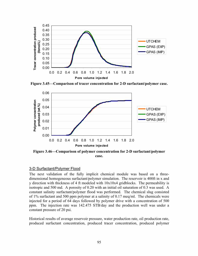
95
0.000.050.100.150.200.250.300.350.400.45
0.0 0.2 0.4 0.6 0.8 1.0 1.2 1.4 1.6 1.8 2.0Pore volume injected
Trac
er c
once
ntra
tion
prod
uced
(lb
mol
/L) UTCHEM
GPAS (EXP)GPAS (IMP)
Figure 3.45—Comparison of tracer concentration for 2-D surfactant/polymer case.
0.00
0.01
0.02
0.03
0.04
0.05
0.06
0.0 0.2 0.4 0.6 0.8 1.0 1.2 1.4 1.6 1.8 2.0Pore volume injected
Poly
mer
con
cent
ratio
n pr
oduc
ed (w
t.%)
UTCHEMGPAS (EXP)GPAS (IMP)
Figure 3.46—Comparison of polymer concentration for 2-D surfactant/polymer
case.
3-D Surfactant/Polymer Flood The next validation of the fully implicit chemical module was based on a three-dimensional homogeneous surfactant/polymer simulation. The reservoir is 400ft in x and y direction with thickness of 4 ft modeled with 10x10x4 gridblocks. The permeability is isotropic and 500 md. A porosity of 0.20 with an initial oil saturation of 0.3 was used. A constant salinity surfactant/polymer flood was performed. The chemical slug consisted of 1% surfactant and 500 ppm polymer at a salinity of 0.17 meq/ml. The chemicals were injected for a period of 64 days followed by polymer drive with a concentration of 500 ppm. The injection rate was 142.475 STB/day and the production well was under a constant pressure of 20 psi. Historical results of average reservoir pressure, water production rate, oil production rate, produced surfactant concentration, produced tracer concentration, produced polymer
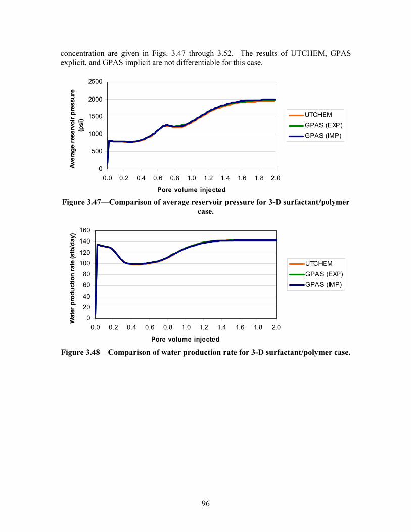
96
concentration are given in Figs. 3.47 through 3.52. The results of UTCHEM, GPAS explicit, and GPAS implicit are not differentiable for this case.
0
500
1000
1500
2000
2500
0.0 0.2 0.4 0.6 0.8 1.0 1.2 1.4 1.6 1.8 2.0
Pore volume injected
Aver
age
rese
rvoi
r pre
ssur
e (p
si) UTCHEM
GPAS (EXP)GPAS (IMP)
Figure 3.47—Comparison of average reservoir pressure for 3-D surfactant/polymer
case.
0
2040
60
80
100120
140
160
0.0 0.2 0.4 0.6 0.8 1.0 1.2 1.4 1.6 1.8 2.0
Pore volume injected
Wat
er p
rodu
ctio
n ra
te (s
tb/d
ay)
UTCHEMGPAS (EXP)GPAS (IMP)
Figure 3.48—Comparison of water production rate for 3-D surfactant/polymer case.
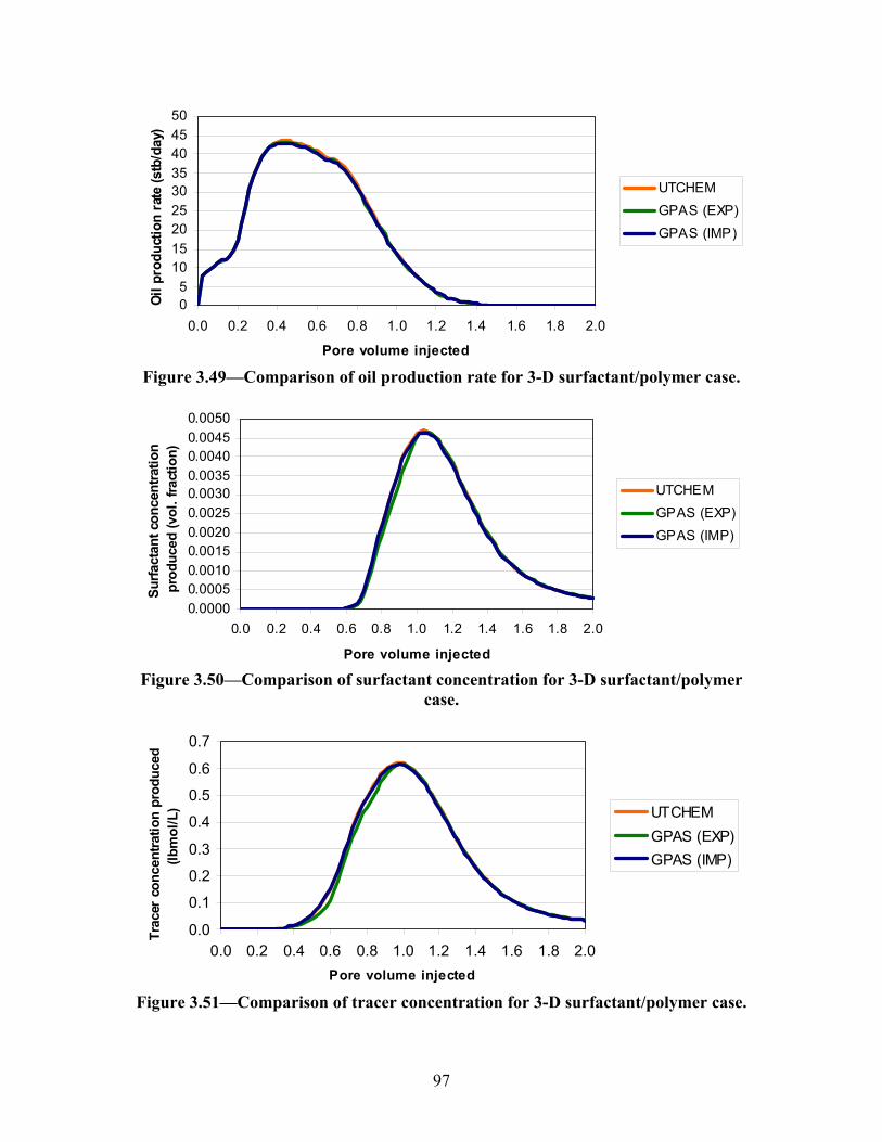
97
05
101520253035404550
0.0 0.2 0.4 0.6 0.8 1.0 1.2 1.4 1.6 1.8 2.0
Pore volume injected
Oil
prod
uctio
n ra
te (s
tb/d
ay)
UTCHEMGPAS (EXP)GPAS (IMP)
Figure 3.49—Comparison of oil production rate for 3-D surfactant/polymer case.
0.00000.00050.00100.00150.00200.00250.00300.00350.00400.00450.0050
0.0 0.2 0.4 0.6 0.8 1.0 1.2 1.4 1.6 1.8 2.0
Pore volume injected
Surfa
ctan
t con
cent
ratio
n pr
oduc
ed (v
ol. f
ract
ion)
UTCHEMGPAS (EXP)GPAS (IMP)
Figure 3.50—Comparison of surfactant concentration for 3-D surfactant/polymer
case.
0.0
0.1
0.2
0.3
0.4
0.5
0.6
0.7
0.0 0.2 0.4 0.6 0.8 1.0 1.2 1.4 1.6 1.8 2.0Pore volume injected
Trac
er c
once
ntra
tion
prod
uced
(lb
mol
/L) UTCHEM
GPAS (EXP)GPAS (IMP)
Figure 3.51—Comparison of tracer concentration for 3-D surfactant/polymer case.
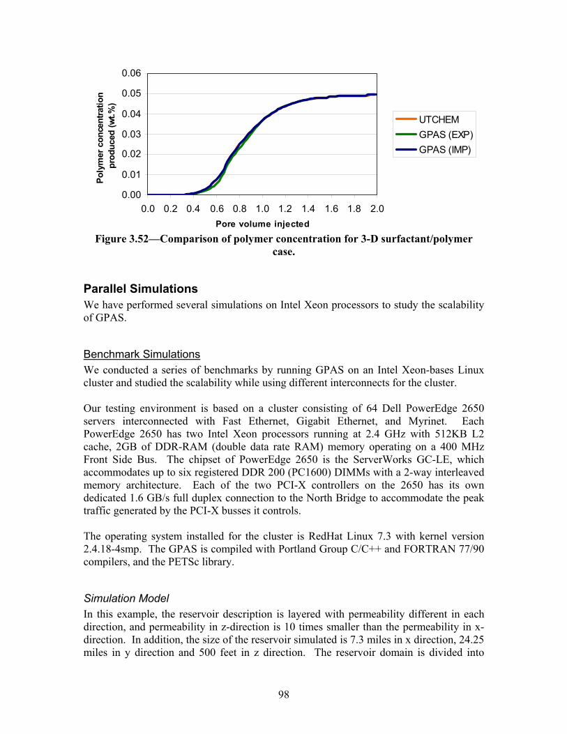
98
0.00
0.01
0.02
0.03
0.04
0.05
0.06
0.0 0.2 0.4 0.6 0.8 1.0 1.2 1.4 1.6 1.8 2.0Pore volume injected
Poly
mer
con
cent
ratio
n pr
oduc
ed (w
t.%)
UTCHEMGPAS (EXP)GPAS (IMP)
Figure 3.52—Comparison of polymer concentration for 3-D surfactant/polymer
case.
Parallel Simulations We have performed several simulations on Intel Xeon processors to study the scalability of GPAS.
Benchmark Simulations We conducted a series of benchmarks by running GPAS on an Intel Xeon-bases Linux cluster and studied the scalability while using different interconnects for the cluster. Our testing environment is based on a cluster consisting of 64 Dell PowerEdge 2650 servers interconnected with Fast Ethernet, Gigabit Ethernet, and Myrinet. Each PowerEdge 2650 has two Intel Xeon processors running at 2.4 GHz with 512KB L2 cache, 2GB of DDR-RAM (double data rate RAM) memory operating on a 400 MHz Front Side Bus. The chipset of PowerEdge 2650 is the ServerWorks GC-LE, which accommodates up to six registered DDR 200 (PC1600) DIMMs with a 2-way interleaved memory architecture. Each of the two PCI-X controllers on the 2650 has its own dedicated 1.6 GB/s full duplex connection to the North Bridge to accommodate the peak traffic generated by the PCI-X busses it controls. The operating system installed for the cluster is RedHat Linux 7.3 with kernel version 2.4.18-4smp. The GPAS is compiled with Portland Group C/C++ and FORTRAN 77/90 compilers, and the PETSc library.
Simulation Model In this example, the reservoir description is layered with permeability different in each direction, and permeability in z-direction is 10 times smaller than the permeability in x-direction. In addition, the size of the reservoir simulated is 7.3 miles in x direction, 24.25 miles in y direction and 500 feet in z direction. The reservoir domain is divided into
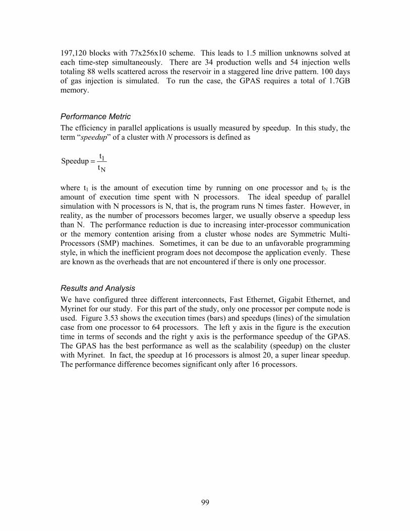
99
197,120 blocks with 77x256x10 scheme. This leads to 1.5 million unknowns solved at each time-step simultaneously. There are 34 production wells and 54 injection wells totaling 88 wells scattered across the reservoir in a staggered line drive pattern. 100 days of gas injection is simulated. To run the case, the GPAS requires a total of 1.7GB memory.
Performance Metric The efficiency in parallel applications is usually measured by speedup. In this study, the term “speedup” of a cluster with N processors is defined as
1
N
tSpeedupt
=
where t1 is the amount of execution time by running on one processor and tN is the amount of execution time spent with N processors. The ideal speedup of parallel simulation with N processors is N, that is, the program runs N times faster. However, in reality, as the number of processors becomes larger, we usually observe a speedup less than N. The performance reduction is due to increasing inter-processor communication or the memory contention arising from a cluster whose nodes are Symmetric Multi-Processors (SMP) machines. Sometimes, it can be due to an unfavorable programming style, in which the inefficient program does not decompose the application evenly. These are known as the overheads that are not encountered if there is only one processor.
Results and Analysis We have configured three different interconnects, Fast Ethernet, Gigabit Ethernet, and Myrinet for our study. For this part of the study, only one processor per compute node is used. Figure 3.53 shows the execution times (bars) and speedups (lines) of the simulation case from one processor to 64 processors. The left y axis in the figure is the execution time in terms of seconds and the right y axis is the performance speedup of the GPAS. The GPAS has the best performance as well as the scalability (speedup) on the cluster with Myrinet. In fact, the speedup at 16 processors is almost 20, a super linear speedup. The performance difference becomes significant only after 16 processors.
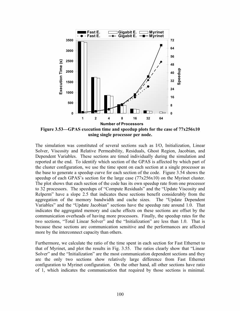
100
0
500
1000
1500
2000
2500
3000
3500
1 2 4 8 16 32 64
Number of Processors
Exec
utio
n Ti
me
(s)
0
8
16
24
32
40
48
56
64
72
Spee
dup
Fast E. Gigabit E. MyrinetFast E. Gigabit E. Myrinet
Figure 3.53—GPAS execution time and speedup plots for the case of 77x256x10
using single processor per node. The simulation was constituted of several sections such as I/O, Initialization, Linear Solver, Viscosity and Relative Permeability, Residuals, Ghost Region, Jacobian, and Dependent Variables. These sections are timed individually during the simulation and reported at the end. To identify which section of the GPAS is affected by which part of the cluster configuration, we use the time spent on each section at a single processor as the base to generate a speedup curve for each section of the code. Figure 3.54 shows the speedup of each GPAS’s section for the large case (77x256x10) on the Myrinet cluster. The plot shows that each section of the code has its own speedup rate from one processor to 32 processors. The speedups of “Compute Residuals” and the “Update Viscosity and Relperm” have a slope 2.5 that indicates these sections benefit considerably from the aggregation of the memory bandwidth and cache sizes. The “Update Dependent Variables” and the “Update Jacobian” sections have the speedup rate around 1.0. That indicates the aggregated memory and cache effects on these sections are offset by the communication overheads of having more processors. Finally, the speedup rates for the two sections, “Total Linear Solver” and the “Initialization” are less than 1.0. That is because these sections are communication sensitive and the performances are affected more by the interconnect capacity than others. Furthermore, we calculate the ratio of the time spent in each section for Fast Ethernet to that of Myrinet, and plot the results in Fig. 3.55. The ratios clearly show that “Linear Solver” and the “Initialization” are the most communication dependent sections and they are the only two sections show relatively large difference from Fast Ethernet configuration to Myrinet configuration. On the other hand, all other sections have ratio of 1, which indicates the communication that required by those sections is minimal.
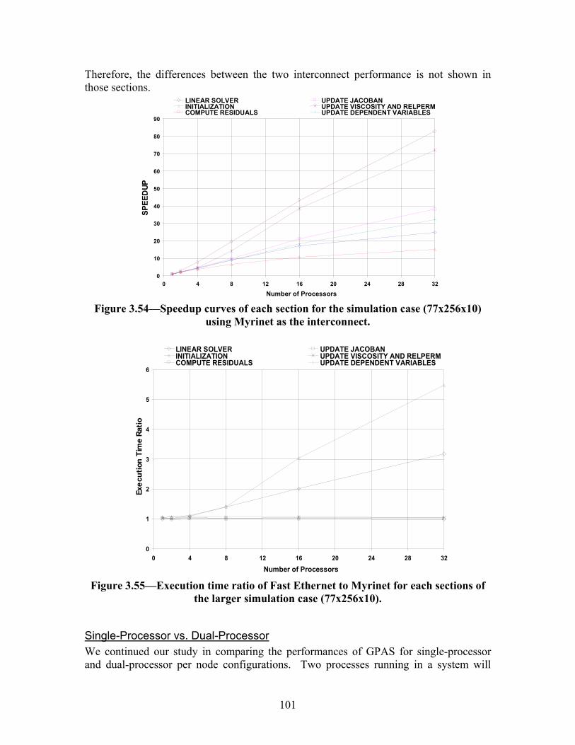
101
Therefore, the differences between the two interconnect performance is not shown in those sections.
0 10 20 30 40 50 60 70 80 90
0 4 8 12 16 20 24 28 32 Number of Processors
Speedup
LINEAR SOLVER UPDATE JACOBANINITIALIZATION UPDATE VISCOSITY AND RELPERM COMPUTE RESIDUALS UPDATE DEPENDENT VARIABLES
SPEE
DUP
Figure 3.54—Speedup curves of each section for the simulation case (77x256x10)
using Myrinet as the interconnect.
0
1
2
3
4
5
6
0 4 8 12 16 20 24 28 32 Number of Processors
Execution Time Ratio
LINEAR SOLVER UPDATE JACOBANINITIALIZATION UPDATE VISCOSITY AND RELPERM COMPUTE RESIDUALS UPDATE DEPENDENT VARIABLES
Exec
utio
n Ti
me
Ratio
Figure 3.55—Execution time ratio of Fast Ethernet to Myrinet for each sections of
the larger simulation case (77x256x10).
Single-Processor vs. Dual-Processor We continued our study in comparing the performances of GPAS for single-processor and dual-processor per node configurations. Two processes running in a system will
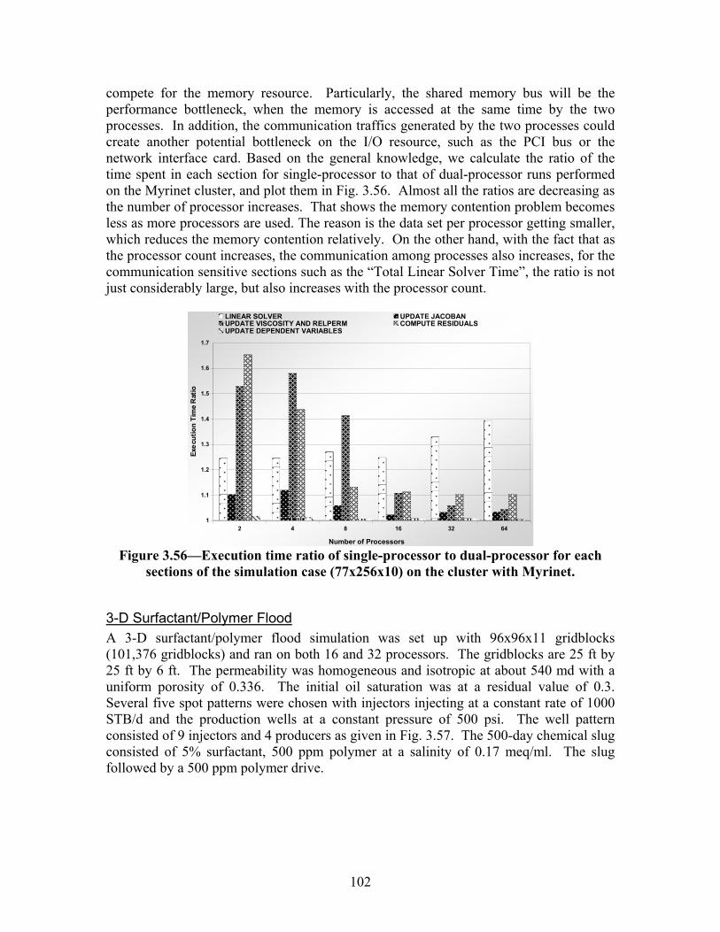
102
compete for the memory resource. Particularly, the shared memory bus will be the performance bottleneck, when the memory is accessed at the same time by the two processes. In addition, the communication traffics generated by the two processes could create another potential bottleneck on the I/O resource, such as the PCI bus or the network interface card. Based on the general knowledge, we calculate the ratio of the time spent in each section for single-processor to that of dual-processor runs performed on the Myrinet cluster, and plot them in Fig. 3.56. Almost all the ratios are decreasing as the number of processor increases. That shows the memory contention problem becomes less as more processors are used. The reason is the data set per processor getting smaller, which reduces the memory contention relatively. On the other hand, with the fact that as the processor count increases, the communication among processes also increases, for the communication sensitive sections such as the “Total Linear Solver Time”, the ratio is not just considerably large, but also increases with the processor count.
1
1.1
1.2
1.3
1.4
1.5
1.6
1.7
2 4 8 16 32 64 Number of Processors
LINEAR SOLVER UPDATE JACOBANUPDATE VISCOSITY AND RELPERM COMPUTE RESIDUALSUPDATE DEPENDENT VARIABLES
Exec
utio
n Ti
me
Rat
io
Figure 3.56—Execution time ratio of single-processor to dual-processor for each
sections of the simulation case (77x256x10) on the cluster with Myrinet.
3-D Surfactant/Polymer Flood A 3-D surfactant/polymer flood simulation was set up with 96x96x11 gridblocks (101,376 gridblocks) and ran on both 16 and 32 processors. The gridblocks are 25 ft by 25 ft by 6 ft. The permeability was homogeneous and isotropic at about 540 md with a uniform porosity of 0.336. The initial oil saturation was at a residual value of 0.3. Several five spot patterns were chosen with injectors injecting at a constant rate of 1000 STB/d and the production wells at a constant pressure of 500 psi. The well pattern consisted of 9 injectors and 4 producers as given in Fig. 3.57. The 500-day chemical slug consisted of 5% surfactant, 500 ppm polymer at a salinity of 0.17 meq/ml. The slug followed by a 500 ppm polymer drive.
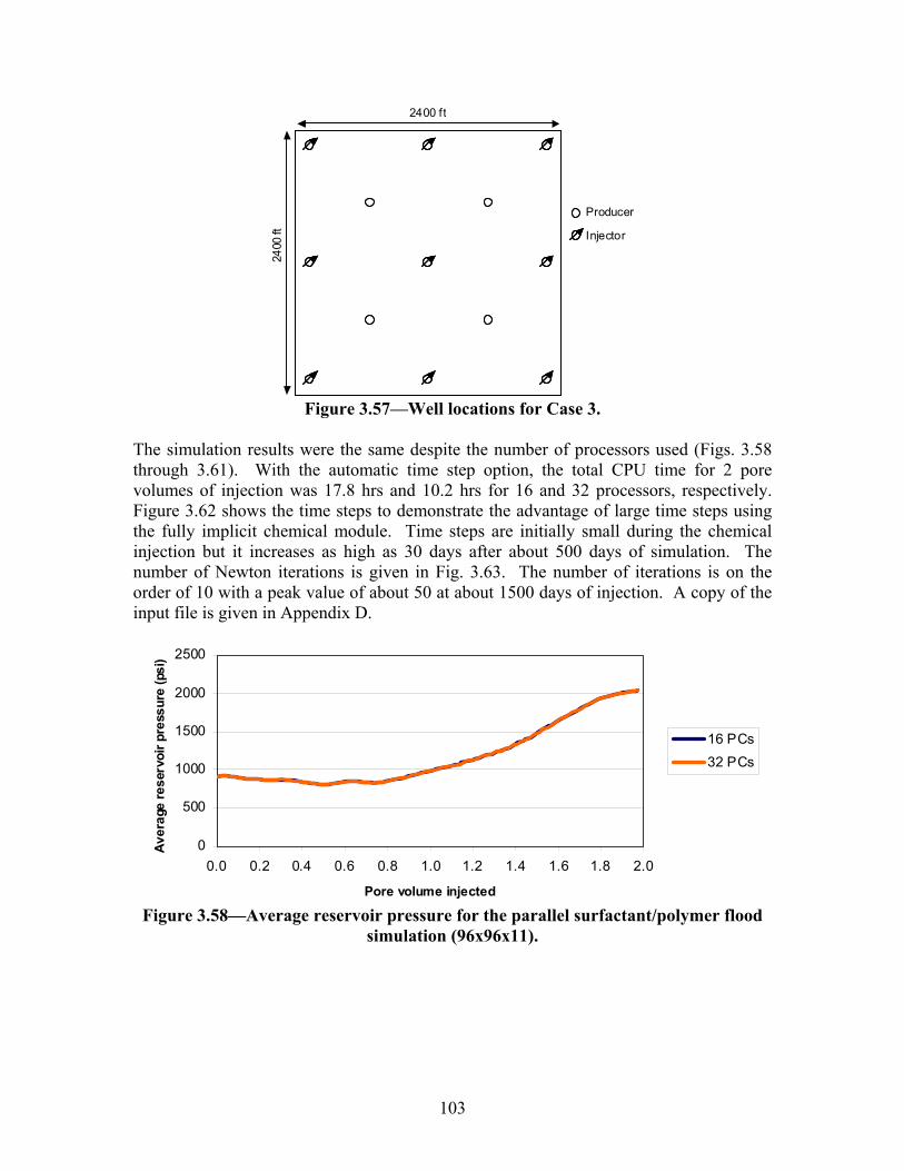
103
2400
ft
2400 ft
Injector
Producer
Figure 3.57—Well locations for Case 3.
The simulation results were the same despite the number of processors used (Figs. 3.58 through 3.61). With the automatic time step option, the total CPU time for 2 pore volumes of injection was 17.8 hrs and 10.2 hrs for 16 and 32 processors, respectively. Figure 3.62 shows the time steps to demonstrate the advantage of large time steps using the fully implicit chemical module. Time steps are initially small during the chemical injection but it increases as high as 30 days after about 500 days of simulation. The number of Newton iterations is given in Fig. 3.63. The number of iterations is on the order of 10 with a peak value of about 50 at about 1500 days of injection. A copy of the input file is given in Appendix D.
0
500
1000
1500
2000
2500
0.0 0.2 0.4 0.6 0.8 1.0 1.2 1.4 1.6 1.8 2.0
Pore volume injected
Aver
age
rese
rvoi
r pre
ssur
e (p
si)
16 PCs32 PCs
Figure 3.58—Average reservoir pressure for the parallel surfactant/polymer flood
simulation (96x96x11).

104
0100020003000400050006000700080009000
10000
0.0 0.2 0.4 0.6 0.8 1.0 1.2 1.4 1.6 1.8 2.0
Pore volume injected
Wat
er p
rodu
ctio
n ra
te (s
tb/d
ay)
16 PCs32 PCs
Figure 3.59—Water production rate for the parallel surfactant/polymer flood
simulation (96x96x11).
0
500
1000
1500
2000
2500
3000
0.0 0.2 0.4 0.6 0.8 1.0 1.2 1.4 1.6 1.8 2.0
Pore volume injected
Oil p
rodu
ctio
n ra
te (s
tb/d
ay)
16 PCs32 PCs
Figure 3.60—Oil production rate for the parallel surfactant/polymer flood
simulation (96x96x11).
0.0
0.1
0.2
0.3
0.4
0.5
0.6
0.7
0.8
0.0 0.2 0.4 0.6 0.8 1.0 1.2 1.4 1.6 1.8 2.0
Pore volume injected
Cum
mul
ativ
e oi
l rec
over
y
16 PCs32 PCs
Figure 3.61—Cumulative oil recovery for the parallel surfactant/polymer flood
simulation (96x96x11).
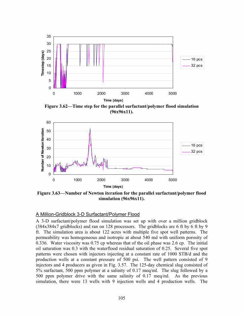
105
0
5
10
15
20
25
30
35
0 1000 2000 3000 4000 5000
Time (days)
Tim
este
p (d
ays)
16 pcs32 pcs
Figure 3.62—Time step for the parallel surfactant/polymer flood simulation
(96x96x11).
0
10
20
30
40
50
60
0 1000 2000 3000 4000 5000
Time (days)
Num
ber o
f New
ton
itera
tion
16 pcs32 pcs
Figure 3.63—Number of Newton iteration for the parallel surfactant/polymer flood
simulation (96x96x11).
A Million-Gridblock 3-D Surfactant/Polymer Flood A 3-D surfactant/polymer flood simulation was set up with over a million gridblock (384x384x7 gridblocks) and ran on 128 processors. The gridblocks are 6 ft by 6 ft by 9 ft. The simulation area is about 122 acres with multiple five spot well patterns. The permeability was homogeneous and isotropic at about 540 md with uniform porosity of 0.336. Water viscosity was 0.75 cp whereas that of the oil phase was 2.6 cp. The initial oil saturation was 0.3 with the waterflood residual saturation of 0.25. Several five spot patterns were chosen with injectors injecting at a constant rate of 1000 STB/d and the production wells at a constant pressure of 500 psi. The well pattern consisted of 9 injectors and 4 producers as given in Fig. 3.57. The 125-day chemical slug consisted of 5% surfactant, 500 ppm polymer at a salinity of 0.17 meq/ml. The slug followed by a 500 ppm polymer drive with the same salinity of 0.17 meq/ml. As the previous simulation, there were 13 wells with 9 injection wells and 4 production wells. The
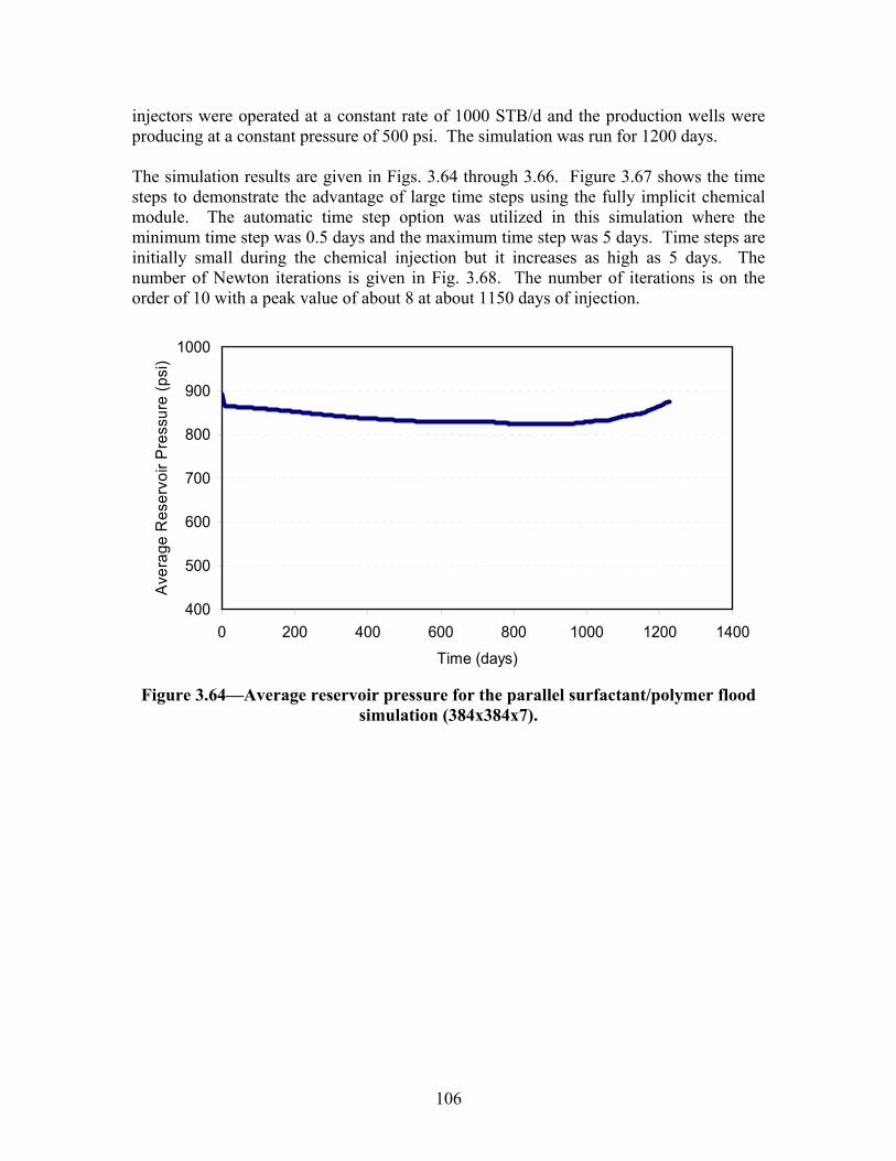
106
injectors were operated at a constant rate of 1000 STB/d and the production wells were producing at a constant pressure of 500 psi. The simulation was run for 1200 days. The simulation results are given in Figs. 3.64 through 3.66. Figure 3.67 shows the time steps to demonstrate the advantage of large time steps using the fully implicit chemical module. The automatic time step option was utilized in this simulation where the minimum time step was 0.5 days and the maximum time step was 5 days. Time steps are initially small during the chemical injection but it increases as high as 5 days. The number of Newton iterations is given in Fig. 3.68. The number of iterations is on the order of 10 with a peak value of about 8 at about 1150 days of injection.
400
500
600
700
800
900
1000
0 200 400 600 800 1000 1200 1400
Time (days)
Ave
rage
Res
ervo
ir P
ress
ure
(psi
)
Figure 3.64—Average reservoir pressure for the parallel surfactant/polymer flood
simulation (384x384x7).
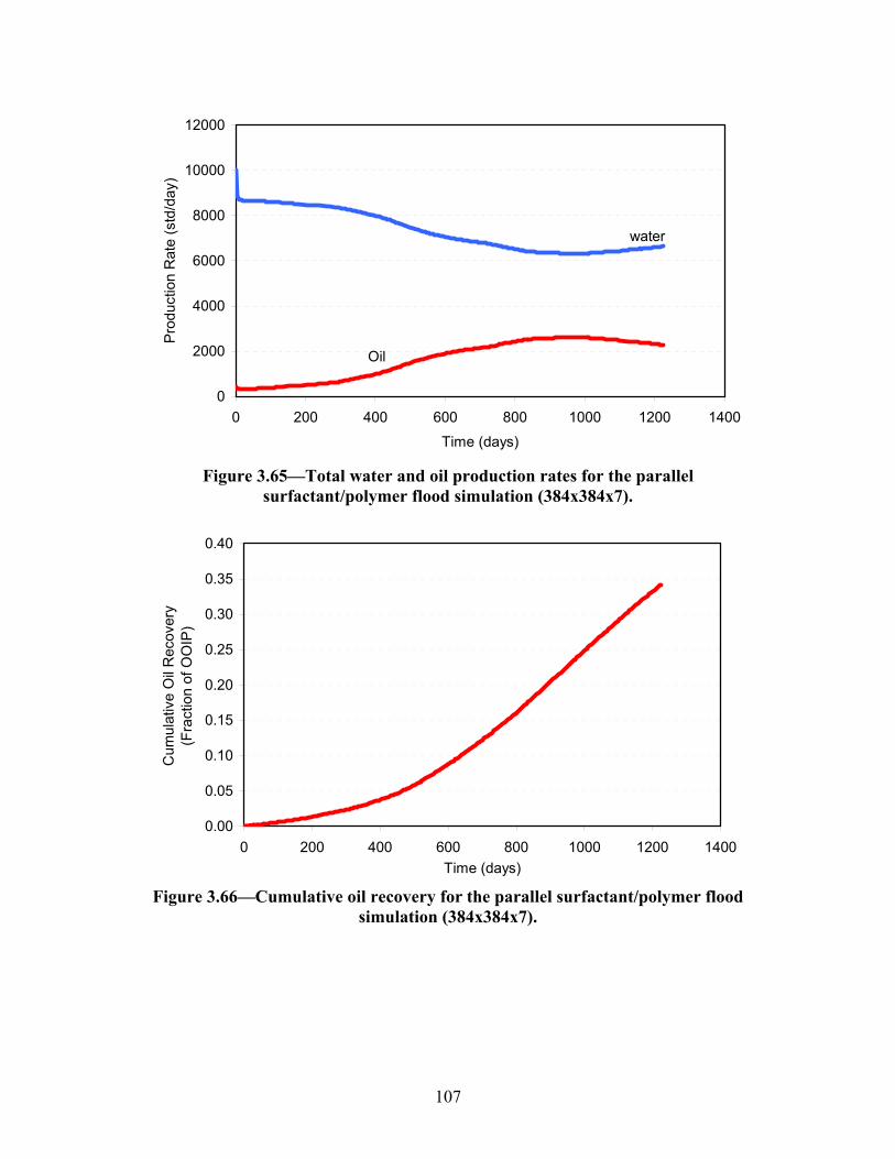
107
0
2000
4000
6000
8000
10000
12000
0 200 400 600 800 1000 1200 1400
Time (days)
Prod
uctio
n R
ate
(std
/day
)
water
Oil
Figure 3.65—Total water and oil production rates for the parallel
surfactant/polymer flood simulation (384x384x7).
0.00
0.05
0.10
0.15
0.20
0.25
0.30
0.35
0.40
0 200 400 600 800 1000 1200 1400Time (days)
Cum
ulat
ive
Oil
Rec
over
y(F
ract
ion
of O
OIP
)
Figure 3.66—Cumulative oil recovery for the parallel surfactant/polymer flood
simulation (384x384x7).
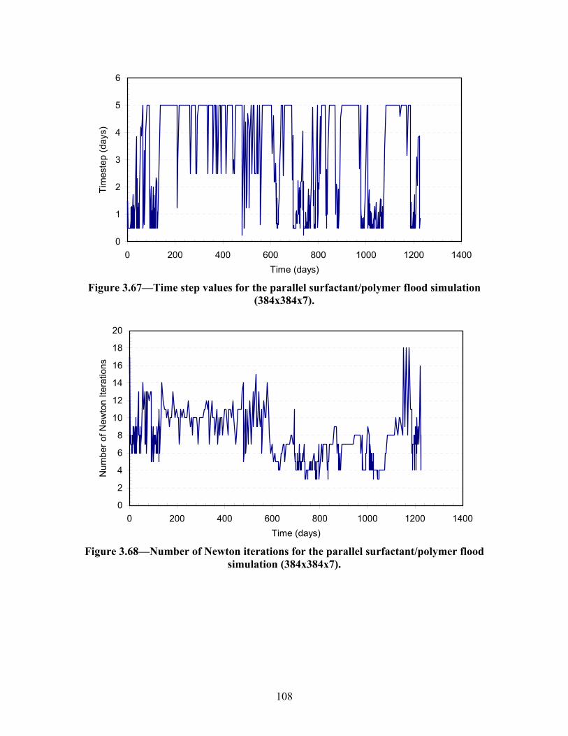
108
0
1
2
3
4
5
6
0 200 400 600 800 1000 1200 1400Time (days)
Tim
este
p (d
ays)
Figure 3.67—Time step values for the parallel surfactant/polymer flood simulation
(384x384x7).
0
2
4
6
8
10
12
14
16
18
20
0 200 400 600 800 1000 1200 1400Time (days)
Num
ber o
f New
ton
Itera
tions
Figure 3.68—Number of Newton iterations for the parallel surfactant/polymer flood
simulation (384x384x7).
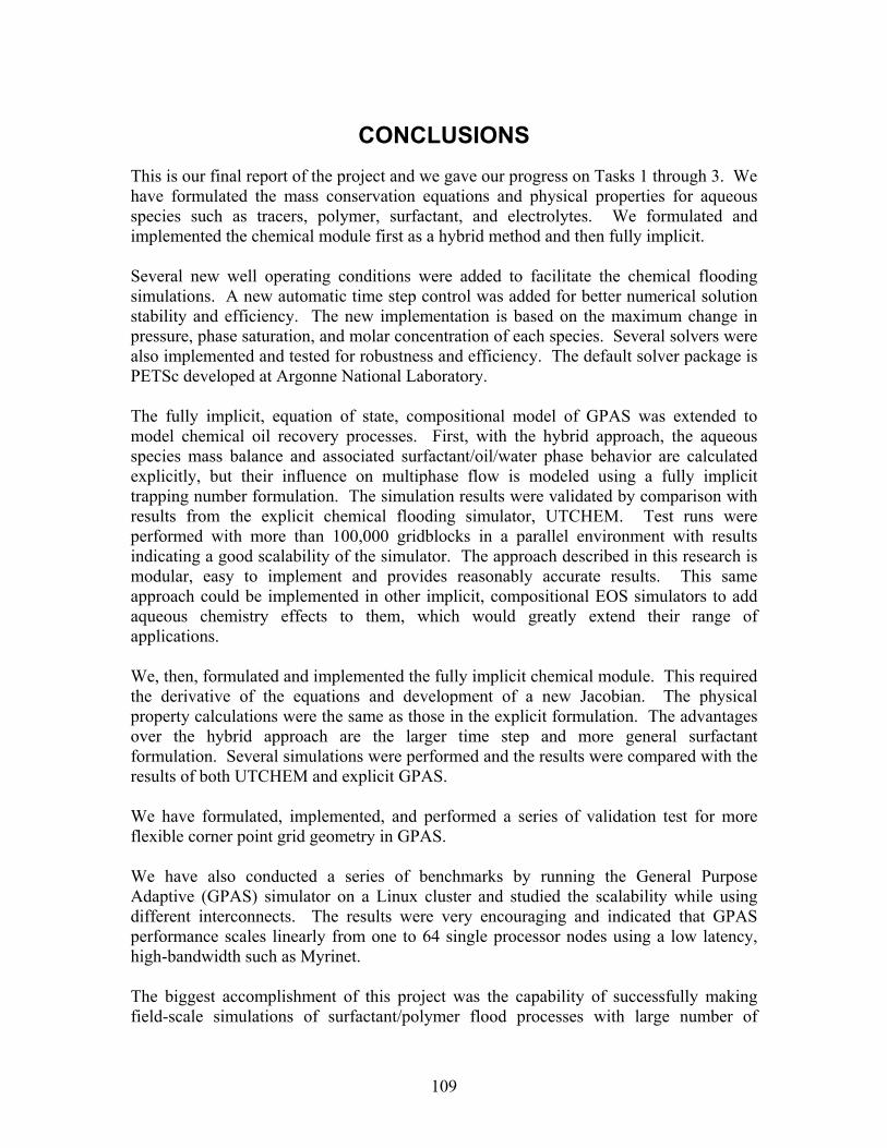
109
CONCLUSIONS This is our final report of the project and we gave our progress on Tasks 1 through 3. We have formulated the mass conservation equations and physical properties for aqueous species such as tracers, polymer, surfactant, and electrolytes. We formulated and implemented the chemical module first as a hybrid method and then fully implicit. Several new well operating conditions were added to facilitate the chemical flooding simulations. A new automatic time step control was added for better numerical solution stability and efficiency. The new implementation is based on the maximum change in pressure, phase saturation, and molar concentration of each species. Several solvers were also implemented and tested for robustness and efficiency. The default solver package is PETSc developed at Argonne National Laboratory. The fully implicit, equation of state, compositional model of GPAS was extended to model chemical oil recovery processes. First, with the hybrid approach, the aqueous species mass balance and associated surfactant/oil/water phase behavior are calculated explicitly, but their influence on multiphase flow is modeled using a fully implicit trapping number formulation. The simulation results were validated by comparison with results from the explicit chemical flooding simulator, UTCHEM. Test runs were performed with more than 100,000 gridblocks in a parallel environment with results indicating a good scalability of the simulator. The approach described in this research is modular, easy to implement and provides reasonably accurate results. This same approach could be implemented in other implicit, compositional EOS simulators to add aqueous chemistry effects to them, which would greatly extend their range of applications. We, then, formulated and implemented the fully implicit chemical module. This required the derivative of the equations and development of a new Jacobian. The physical property calculations were the same as those in the explicit formulation. The advantages over the hybrid approach are the larger time step and more general surfactant formulation. Several simulations were performed and the results were compared with the results of both UTCHEM and explicit GPAS. We have formulated, implemented, and performed a series of validation test for more flexible corner point grid geometry in GPAS. We have also conducted a series of benchmarks by running the General Purpose Adaptive (GPAS) simulator on a Linux cluster and studied the scalability while using different interconnects. The results were very encouraging and indicated that GPAS performance scales linearly from one to 64 single processor nodes using a low latency, high-bandwidth such as Myrinet. The biggest accomplishment of this project was the capability of successfully making field-scale simulations of surfactant/polymer flood processes with large number of

110
gridblocks on the order of one million with a fully implicit formulation and parallel capability on a cluster of PCs
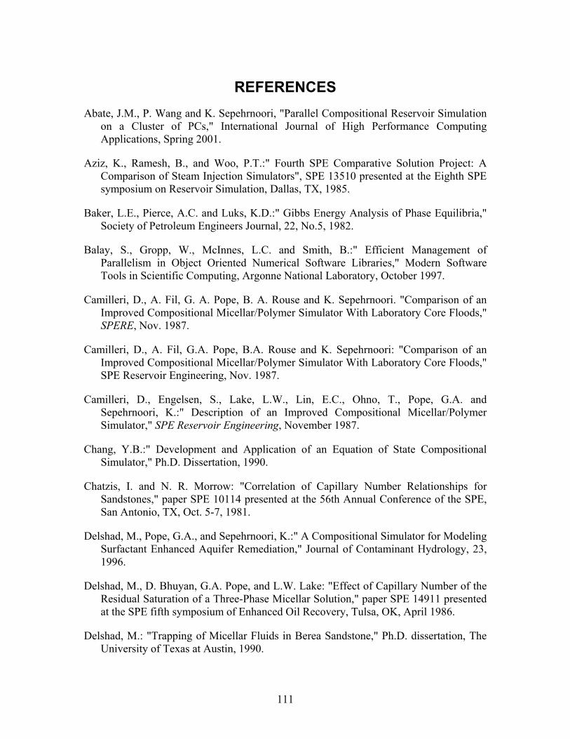
111
REFERENCES Abate, J.M., P. Wang and K. Sepehrnoori, "Parallel Compositional Reservoir Simulation
on a Cluster of PCs," International Journal of High Performance Computing Applications, Spring 2001.
Aziz, K., Ramesh, B., and Woo, P.T.:" Fourth SPE Comparative Solution Project: A Comparison of Steam Injection Simulators", SPE 13510 presented at the Eighth SPE symposium on Reservoir Simulation, Dallas, TX, 1985.
Baker, L.E., Pierce, A.C. and Luks, K.D.:" Gibbs Energy Analysis of Phase Equilibria," Society of Petroleum Engineers Journal, 22, No.5, 1982.
Balay, S., Gropp, W., McInnes, L.C. and Smith, B.:" Efficient Management of Parallelism in Object Oriented Numerical Software Libraries," Modern Software Tools in Scientific Computing, Argonne National Laboratory, October 1997.
Camilleri, D., A. Fil, G. A. Pope, B. A. Rouse and K. Sepehrnoori. "Comparison of an Improved Compositional Micellar/Polymer Simulator With Laboratory Core Floods," SPERE, Nov. 1987.
Camilleri, D., A. Fil, G.A. Pope, B.A. Rouse and K. Sepehrnoori: "Comparison of an Improved Compositional Micellar/Polymer Simulator With Laboratory Core Floods," SPE Reservoir Engineering, Nov. 1987.
Camilleri, D., Engelsen, S., Lake, L.W., Lin, E.C., Ohno, T., Pope, G.A. and Sepehrnoori, K.:" Description of an Improved Compositional Micellar/Polymer Simulator," SPE Reservoir Engineering, November 1987.
Chang, Y.B.:" Development and Application of an Equation of State Compositional Simulator," Ph.D. Dissertation, 1990.
Chatzis, I. and N. R. Morrow: "Correlation of Capillary Number Relationships for Sandstones," paper SPE 10114 presented at the 56th Annual Conference of the SPE, San Antonio, TX, Oct. 5-7, 1981.
Delshad, M., Pope, G.A., and Sepehrnoori, K.:" A Compositional Simulator for Modeling Surfactant Enhanced Aquifer Remediation," Journal of Contaminant Hydrology, 23, 1996.
Delshad, M., D. Bhuyan, G.A. Pope, and L.W. Lake: "Effect of Capillary Number of the Residual Saturation of a Three-Phase Micellar Solution," paper SPE 14911 presented at the SPE fifth symposium of Enhanced Oil Recovery, Tulsa, OK, April 1986.
Delshad, M.: "Trapping of Micellar Fluids in Berea Sandstone," Ph.D. dissertation, The University of Texas at Austin, 1990.
112
Delshad, M.: Trapping of Micellar Fluids in Berea Sandstone, Ph.D. Dissertation, The University of Texas at Austin, 1990.
Dogru, A.H., H.A. Sunaidi, L.S. Fung, W.A. Habiballah, N. Al-Zamel, and K.G. Li: "A Parallel Reservoir Simulator for Large-Scale Reservoir Simulation," SPEREE, February 2002.
Flory, P.J.: Principles of Polymer Chemistry, Ithaca, New York, Cornell University Press, 1953.
Gai X., R.H. Dean, M.F. Wheeler and R. Liu: "Coupled Geomechanical and Reservoir Modeling on Parallel Computers," paper SPE 79700 presented at the SPE Reservoir Simulation Symposium, Houston, Texas, U.S.A., 3-5 February 2003.
Gosset, H. and Kalitventzeff.:" An Efficient Algorithm to Solve Cubic Equations of State," Fluid Phase Equilibria, 25 ,1986.
Gropp, W., Morgan, T., Smith, B., Arbogast, T., Dawson, C.N., Lake, L.L., McKinney, D.C., Pope, G.A., Sepehrnoori, K., and Wheeler, M.F.: New Generation Framework For Petroleum Reservoir Simulation, First Annul Report, May 31, 1996, Advanced Computational Technology Initiative, Argonne National Laboratory and The University of Texas at Austin.
Habiballah, W.A., M.E. Hayder, M.S. Khan, K.M. Issa, S.H. Zahrani, R.A. Shaikh, A.H. Uwaiyedh, T.P. Tyraskis and M.A. Baddourah: "Parallel Reservoir Simulation Utilizing PC-Clusters in Massive Reservoir Simulation Models," paper SPE 84065 presented at the SPE Annual Technical Conference and Exhibition, Denver, Colorado, U.S.A., 5-8 October 2003.
Hand, D.B.: "Dineric Distribution: I. The Distribution of a Consolute Liquid between Two Immiscible Liquids," Journal of Physics and Chemistry, 34, 1939.
Hirasaki, G. J. and G. A. Pope. "Analysis of Factors Influencing Mobility and Adsorption in the Flow of Polymer Solution Through Porous Media," SPEJ, 337-346, Aug. 1974.
Hirasaki, G.J.: "Application of The Theory of Multicomponent, multiphase displacement to three-component, two-phase surfactant Flooding," SPEJ, 191-204, 1981.
Huh, C.: "Interfacial Tension and Solubilization Ability of a Microemulsion Phase that Coexists with Oil and Brine," Journal of Colloid Interface Science, 71, 1979.
Jin, M.: "A Study of Non-Aqueous Phase Liquid Characterization and Surfactant Remediation," PhD dissertation, University of Texas at Austin. 1995.
John, A.K: " Development of a hybrid approach to couple chemical and compositional models in an implicit, parallel simulator" M.S. thesis, The University of Texas at Austin. 2003.
113
Killough, J.E. and Kossack, C.A.:" Fifth Comparative Solution Project: Evaluation of Miscible Flood Simulators," SPE 16000, presented at the ninth SPE symposium on Reservoir Simulation held in San Antonio, Texas, February, 1987.
Leibovici, C.F. and Neoschil, J.:" A New Look at the Rachford-Rice Equation for Flash Calculations," Fluid Phase Equilibria, 1992.
Lohrenz, J., Bray, B.G. and Clark, C.R.: "Calculating Viscosities of Reservoir Fluids from their Compositions," Trans., AIME, 1964.
Maliska, C.R., Computational Heat Transfer and Fluid Mechanics, 2nd Ed., LTC, Rio de Janeiro, 2004, Brazil. (In Portuguese).
Michelsen, J.L.:" The Isothermal Flash Problem. Part I. Stability," Fluid Phase Equilibrium, 1982.
Morrow, N.R., I. Chatzis and H. Lim: "Relative Permeabilities at Reduced Residual Saturation," J. Can. Pet. Techol., 62-69, Jul-Aug., 1985.
Nalla, G: "Implementation of the chemical flooding module in GPAS," M.S. thesis, The University of Texas at Austin. 2002.
Nelson, R. C. and G. A. Pope. "Phase Relationships in Chemical Flooding," SPEJ, 18,325-338, Trans. AIME, 265, Oct. 1978.
Parashar M., J.A. Wheeler, G. Pope, K. Wang and P. Wang: "A New Generation EOS Compositional Reservoir Simulator: Part II - Framework and Multiprocessing," paper SPE 37977 presented at the SPE Reservoir Simulation Symposium, Dallas, TX., Jun. 8-11, 1997.
Peng, D.Y. and Robinson, D.B." A New Two-Constant Equation of State," Ind. Eng. Chem. Fundam., 1976.
Perschke, D.R.:" Equation of State Phase Behavior Modeling for Compositional Simulator," Ph.D. Dissertation, University of Texas at Austin, 1988.
Pope, G.A., W. Wu, G. Narayanaswamy, M. Delshad, M.M. Sharma and P. Wang: "Modeling Relative Permeability Effects in Gas-Condensate Reservoirs," SPE Reservoir Evaluation & Engineering, April, 2000.
Prouvost, L., G. A. Pope and B. A. Rouse. "Microemulsion Phase Behavior: A Thermodynamic Modeling of the Phase Partitioning of Amphiphilic Species," SPEJ, 693-703, Oct. 1985.
Reed, R. L. and R. N. Healy.. "Some Physico-Chemical Aspects of Microemulsion Flooding: A Review," Improved Oil recovery by Surfactant and Polymer Flooding, D. O. Shah and R. S. Schechter(eds.), Academic Press, New York. 1977.
114
Reid, R.C., Prausnitz, J.M. and Poling, B.E.: The Properties of Gases and Liquids, Fourth Edition, McGraw-Hill, Inc., NY, 1987.
Sandler, Stanley I.: Chemical and Engineering Thermodynamics, Third Edition, John Wiley & Sons, Inc., 1999.
Thompson, J. F., Warsi, Z.U.A, and Mastin C. W., Numerical Grid Generation – Foundations and Applications, Elsevier Science Publishing, New York, 1985.
Trangenstein, J.A.," Customized Minimized Techniques for Phase Equilibrium Computations in Reservoir Simulation," Chem. Eng. Sci., 42, No.12, 1987.
Uetani T., B. Guler, and K. Sepehrnoori, "Reservoir Simulation on High Performance Clusters," presented at the Sixth World Multiconference on Systematics, Cybernetics, and Informatics, Orlando, FL, 14-18 July, 2002.
Wang, P., I. Yotov, M Wheeler, T. Arbogast, C. Dawson, M. Parashar and K. Sepehrnoori: "A New Generation EOS Compositional Reservoir Simulator: Part I - Formulation and Discretization," paper SPE 37979 presented at the SPE Reservoir Simulation Symposium, Dallas, TX, June 1997.
Wang, P., Balay, S., Sepehrnoori, K., Wheeler, J., Abate, J., Smith, B. and Pope, G.A.:" A Fully Implicit Parallel EOS.Compositional Simulator for Large Scale Reservoir Simulation," SPE 51885 presented at the 1999 SPE 15th Reservoir Simulation Symposium, Houston, TX, Feb. 14-17, 1999.
Winsor, P. A. Solvent Properties of Amphiphilic Compounds , Butterworths, London. 1954. Zhang, K., Y.S. Wu, C. Ding, K. Pruess and E. Elmroth: "Parallel Computing Techniques for Large-Scale Reservoir Simulation of Multi-Component and Multiphase Fluid Flow," paper SPE 66343 presented at the SPE Reservoir Simulation Symposium, Houston, Texas, 11-14 February 2001.
115
NOMENCLATURE
p1, p2, p3 pA A A ,S viscosity model parameters for polymer
a Chun-Huh IFT correlation parameter
31, 31, 3a a b adsorption model parameters for surfactant
41, 41, 4a a b adsorption model parameters for polymer
iC volume of ith component in fluid per fluid volume, fraction
iC overall volume of ith component per pore volume, fraction
iC adsorbed volume of ith component per pore volume, fraction
fiC volume of ith component in fluid per pore volume, fraction
ijC volume of ith component in jth phase per volume of jth phase, fraction
SEC effective salinity, meq/ml
SEOPC Optimum salinity, meq/ml
3max,sC height of binodal curve at salinity s
43C concentration of polymer in aqueous or microemulsion phase, wt.%
CMC critical micelle concentration
c Chun-Huh IFT correlation parameter
ic compressibility of ith component, psi-1
oic compressibility of ith component at reference pressure, psi-1
i,injc injected concentration of ith component in aqueous phase; vol. fraction (surfactant), wt.% (polymer), meq/ml (salt), lbmol/L (tracer)
fc compressibility of formation, psi-1
D depth, ft
g gravity acceleration, ft/day2
J Jacobian matrix
i, jJ Jacobian matrix for ith gridblock with respect to unknowns of jth gridblock
116
iK equilibrium ratio for ith component, i i iK y / x=
k absolute permeability, md
k absolute permeability tensor
k transmissibility, md•ft
rjk relative permeability of jth phase, fraction
xk absolute permeability in x direction, md
yk absolute permeability in y direction, md
zk absolute permeability in z direction, md
jL ratio of moles in jth phase to the total number of moles in the mixture
iM molecular weight of ith component, lb/lbmol
jM average molecular weight of jth phase, lb/lbmol
iN mole of ith component per pore volume, lbmol/ft3
iN flux vector of ith species in units of mass of i per surface area-time
fiN mole of ith component in fluid per pore volume, lbmol/ft3
oil,3N mole of hydrocarbons in microemulsion phase per pore volume, lbmol//ft3
T,3N mole of all the components in microemulsion phase per pore volume, lbmol//ft3
jtN trapping number of jth phase, fraction
an total number of aqueous components
bn total number of gridblocks
cn total number of hydrocarbon components
jn relative permeability exponent of jth phase
P fluid pressure, psi oP reference pressure, psi
jP fluid pressure for jth gridblock or jth phase, psi
wfP well bottomhole pressure, psi
117
iq sink(-) or source(+) of ith component, lbmol/day
R residual vector
iR residual vector for ith gridblock
iR mass rate of production in units of mass of i per bulk volume-time
i,mR residual of material balance equation of ith component, lbmol/day
i, jmR residual of material balance equation of ith component for jth
gridblock, lbmol/day
vR residual of volume constraint
ivR residual of volume constraint for ith gridblock
or equivalent well gridblock radius, ft
wr well radius, ft
jS saturation of jth phase, fraction
jrS residual saturation of jth phase, fraction
pS polymer viscosity correlation parameter, dimensionless
T temperature, °F
t time, day
ju flux of jth phase, ft/day
V primary variable
(I)V primary variable at (I,J,K) gridblock at new time level
(I 1)V + primary variable at (I+1,J,K) gridblock at new time level
(I 1)V − primary variable at (I-1,J,K) gridblock at new time level
bV bulk volume for a cell, ft3
pV pore volume for a cell, ft3
jv molar volume of phase j, ft3
iW overall concentration of i in units of mass of i per unit bulk volume
ix mole fraction of ith component in liquid phase
x solution vector
118
ix solution vector for ith gridblock
ijx mole fraction of ith component in jth phase, fraction
x∆ length in x direction of a gridblock, ft
iy mole fraction of ith component in gaseous phase
y∆ length in y direction of a gridblock, ft
z∆ length in z direction of a gridblock, ft
1, 2, 3, 4, 5α α α α α microemulsion viscosity correlation parameters
∆ difference operator
jγ specific gravity of jth phase, psi/ft
Φ flow potential
φ porosity, fraction
rφ porosity at reference pressure, fraction
rjλ relative mobility of jth phase
jµ viscosity of jth phase, cp
jρ mass density of jth phase, lb/ft3
sρ mass density of stationary phase s, lb/ft3
owσ interfacial tension between oleic and aqueous phases, dyne/cm
23σ interfacial tension between oleic and microemulsion phases, dyne/cm
jτ trapping number model parameter of jth phase
ijω mass fraction of ith component in jth phase
iξ molar density of ith component, lbmol/ft3
oiξ molar density of ith component at reference pressure, lbmol/ft3
jξ molar density of jth phase, lbmol/ft3
oξ overall molar density of hydrocarbon components, lbmol/ft3
∇ gradient operator
∇ • divergence operator
119
Superscript High high trapping number
Low low trapping number
O endpoint
n old time level
n+1 new time level
new after update by Newton iteration
old before update by Newton iteration
Subscript i index for component
for iC , iC , iC , fiC , and ijC
1: water, 2: oil, 3: surfactant, 4: polymer, 5: salt
for other symbols 1 to cn : hydrocarbon component cn +1 to cn + an : aqueous component except water 2H O : water o: oil poly: polymer salt: salt surf: surfactant trac: tracer
j index for phase 1: aqueous phase (hybrid model) 2: oleic phase 3: gas (EOS model), microemulsion phase (hybrid model),
aqueous or microemulsion phase (fully implicit model), displaced phase (trapping number calculations)
j' displacing phase for trapping number calculations
s salinity level (0: low, 1: optimal)
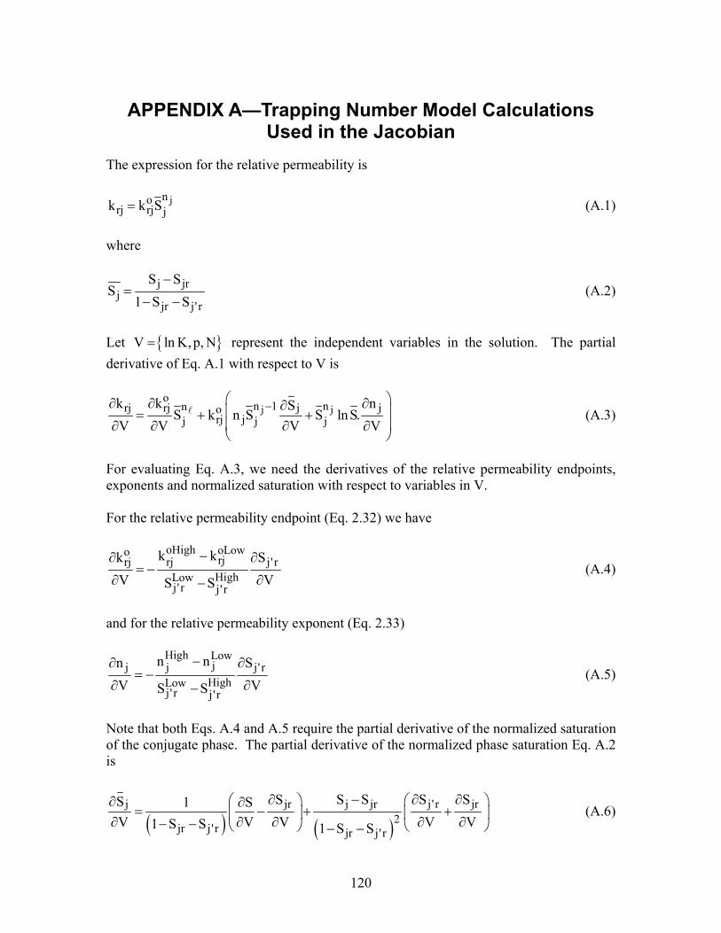
120
APPENDIX A—Trapping Number Model Calculations Used in the Jacobian
The expression for the relative permeability is
jnorj rj jk k S= (A.1)
where
j jrj
jr j' r
S SS
1 S S−
=− −
(A.2)
Let V ln K, p, N= represent the independent variables in the solution. The partial derivative of Eq. A.1 with respect to V is
j jo
n 1 nnrj rj j jorj jj j j
k k nSS k n S S lnS.
V V V V− ∂ ∂ ∂∂ = + +
∂ ∂ ∂ ∂
(A.3)
For evaluating Eq. A.3, we need the derivatives of the relative permeability endpoints, exponents and normalized saturation with respect to variables in V. For the relative permeability endpoint (Eq. 2.32) we have
oHigh oLoworjrj rj j' rHighLow
j' r j' r
k kk SV VS S
−∂ ∂= −
∂ ∂− (A.4)
and for the relative permeability exponent (Eq. 2.33)
High Lowjj j j' r
HighLowj' r j' r
n nn SV VS S
−∂ ∂= −
∂ ∂− (A.5)
Note that both Eqs. A.4 and A.5 require the partial derivative of the normalized saturation of the conjugate phase. The partial derivative of the normalized phase saturation Eq. A.2 is
( ) ( )j jr j jr j' r jr
2jr j' r jr j' r
S S S S SS 1 SV V V V V1 S S 1 S S
∂ − ∂ ∂ ∂ ∂= − + + ∂ ∂ ∂ ∂ ∂− − − −
(A.6)
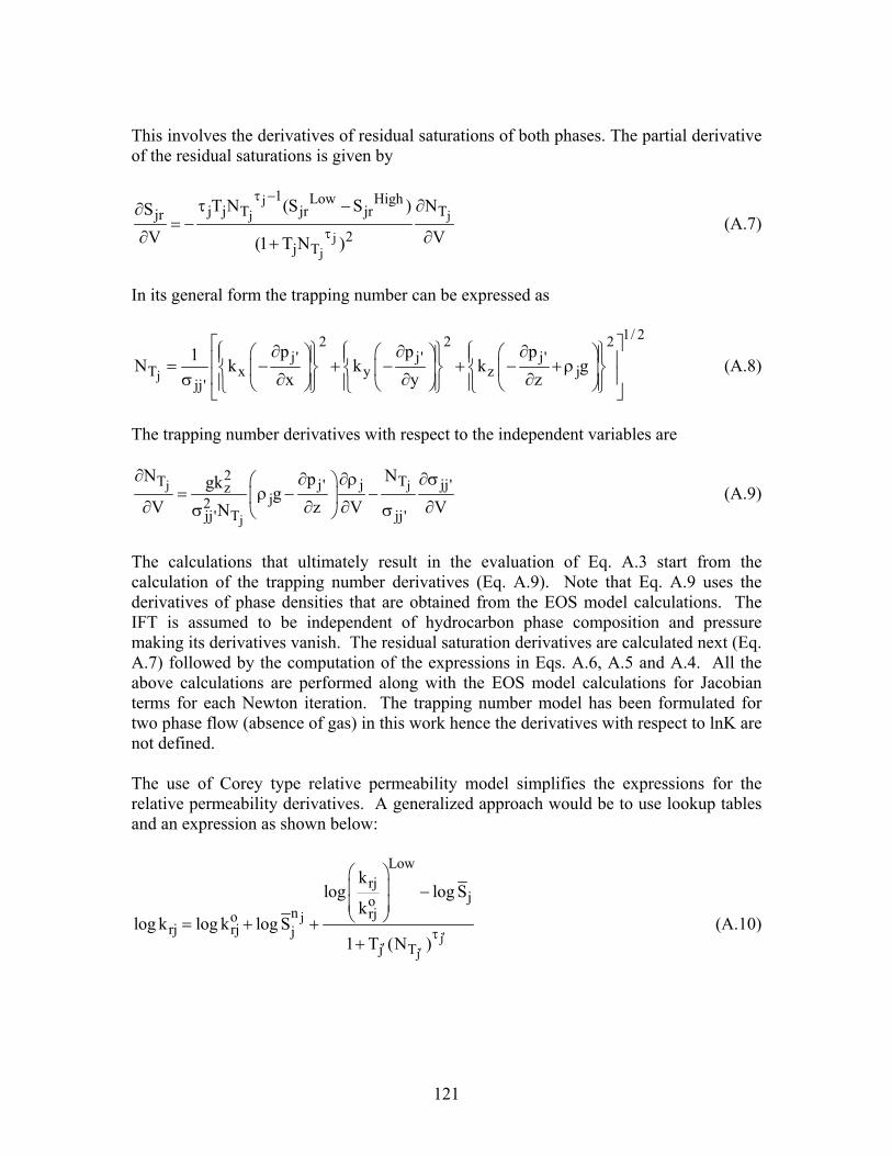
121
This involves the derivatives of residual saturations of both phases. The partial derivative of the residual saturations is given by
jj j
jj
1 Low Highj j T jr jr Tjr
2j T
T N (S S ) NSV V(1 T N )
τ −
τ
τ − ∂∂= −
∂ ∂+ (A.7)
In its general form the trapping number can be expressed as
j
1/ 22 2 2j' j ' j'
T x y z jjj'
p p p1N k k k gx y z
∂ ∂ ∂ = − + − + − + ρ σ ∂ ∂ ∂
(A.8)
The trapping number derivatives with respect to the independent variables are
j j
j
2T Tj' j jj 'zj2
jj' T jj'
N Npgk gV z V VN
∂ ∂ ∂ρ ∂σ = ρ − − ∂ ∂ ∂ ∂σ σ
(A.9)
The calculations that ultimately result in the evaluation of Eq. A.3 start from the calculation of the trapping number derivatives (Eq. A.9). Note that Eq. A.9 uses the derivatives of phase densities that are obtained from the EOS model calculations. The IFT is assumed to be independent of hydrocarbon phase composition and pressure making its derivatives vanish. The residual saturation derivatives are calculated next (Eq. A.7) followed by the computation of the expressions in Eqs. A.6, A.5 and A.4. All the above calculations are performed along with the EOS model calculations for Jacobian terms for each Newton iteration. The trapping number model has been formulated for two phase flow (absence of gas) in this work hence the derivatives with respect to lnK are not defined. The use of Corey type relative permeability model simplifies the expressions for the relative permeability derivatives. A generalized approach would be to use lookup tables and an expression as shown below:
jj
j
Lowrj
jon rjo
rj rj jj T
klog log S
klog k log k log S
1 T (N ) ′′
τ′
− = + ++
(A.10)
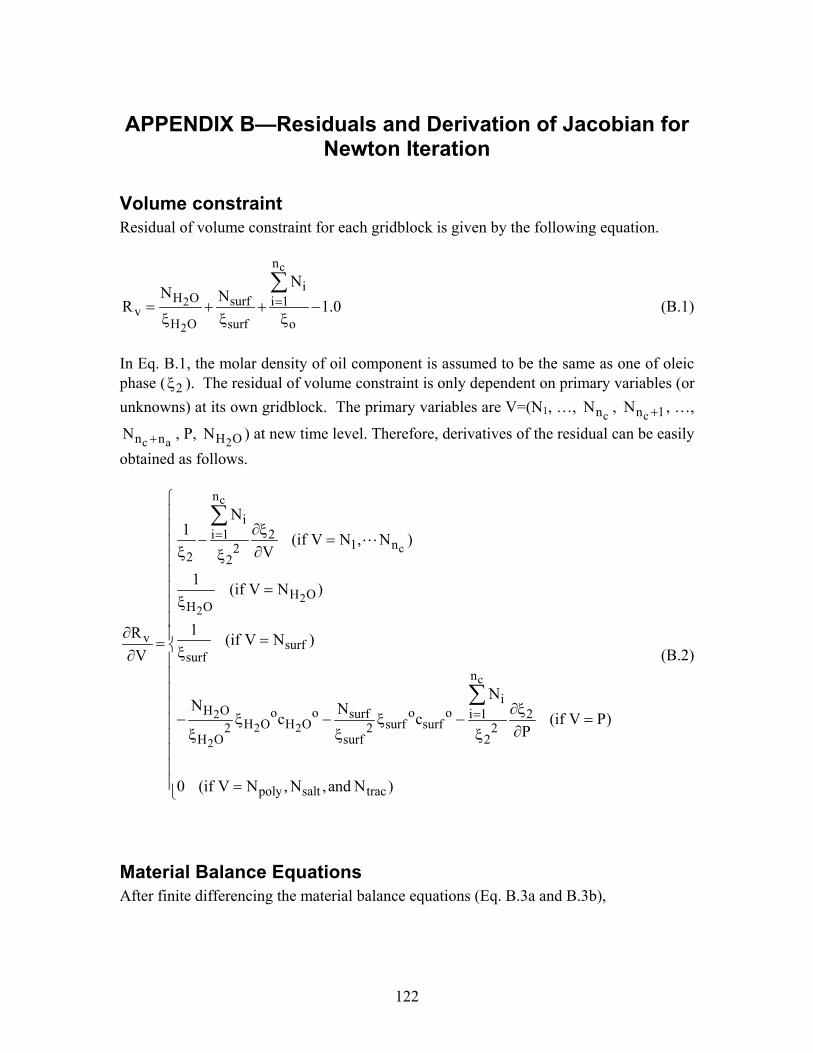
122
APPENDIX B—Residuals and Derivation of Jacobian for Newton Iteration
Volume constraint Residual of volume constraint for each gridblock is given by the following equation.
c
2
2
n
iH O surf i 1
vH O surf o
NN NR 1.0== + + −ξ ξ ξ
∑ (B.1)
In Eq. B.1, the molar density of oil component is assumed to be the same as one of oleic phase ( 2ξ ). The residual of volume constraint is only dependent on primary variables (or unknowns) at its own gridblock. The primary variables are V=(N1, …, cnN , cn 1N + , …,
c an nN + , P, 2H ON ) at new time level. Therefore, derivatives of the residual can be easily obtained as follows.
c
c
22
c
22 2
2
n
ii 1 2
1 n22 2
H OH O
v surfsurf
n
iH O o o o osurf i 1 2
H O H O surf surf2 2 2H O surf 2
poly salt trac
N1 (if V N , N )
V
1 (if V N )
1R (if V N )V
NN Nc c (if V P)
P
0 (if V N , N ,and N )
=
=
∂ξ
− =ξ ∂ξ
=ξ
∂ == ξ∂
∂ξ
− ξ − ξ − = ∂ξ ξ ξ =
∑
∑
(B.2)
Material Balance Equations After finite differencing the material balance equations (Eq. B.3a and B.3b),
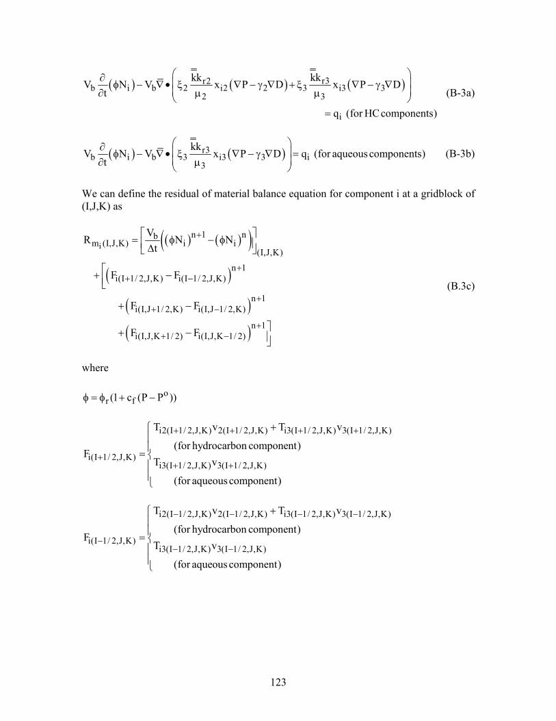
123
( ) ( ) ( )r3r2b i b 2 i2 2 3 i3 3
2 3
i
kkkkV N V x P D x P Dt
q (for HCcomponents)
∂ φ − ∇ • ξ ∇ − γ ∇ + ξ ∇ − γ ∇ ∂ µ µ
=
(B-3a)
( ) ( )r3b i b 3 i3 3 i
3
kkV N V x P D q (for aqueous components)
t
∂ φ − ∇ • ξ ∇ − γ ∇ = ∂ µ
(B-3b)
We can define the residual of material balance equation for component i at a gridblock of (I,J,K) as
( ) ( )( )( )
( )( )
in 1 nb
m (I,J,K) i i(I,J,K)
n 1i(I 1/ 2,J,K) i(I 1/ 2,J,K)
n 1i(I,J 1/ 2,K) i(I,J 1/ 2,K)
n 1i(I,J,K 1/ 2) i(I,J,K 1/ 2)
VR N Nt
F F
F F
F F
+
++ −
++ −
++ −
= φ − φ ∆
+ −
+ −
+ −
(B.3c)
where
or f(1 c (P P ))φ = φ + −
i2(I 1/ 2,J,K) 2(I 1/ 2,J,K) i3(I 1/ 2,J,K) 3(I 1/ 2,J,K)
i(I 1/ 2,J,K)i3(I 1/ 2,J,K) 3(I 1/ 2,J,K)
T v T v
(for hydrocarbon component)F
T v
(for aqueous component)
+ + + +
++ +
+=
i2(I 1/ 2,J,K) 2(I 1/ 2,J,K) i3(I 1/ 2,J,K) 3(I 1/ 2,J,K)
i(I 1/ 2,J,K)i3(I 1/ 2,J,K) 3(I 1/ 2,J,K)
T v T v
(for hydrocarbon component)F
T v
(for aqueous component)
− − − −
−− −
+=
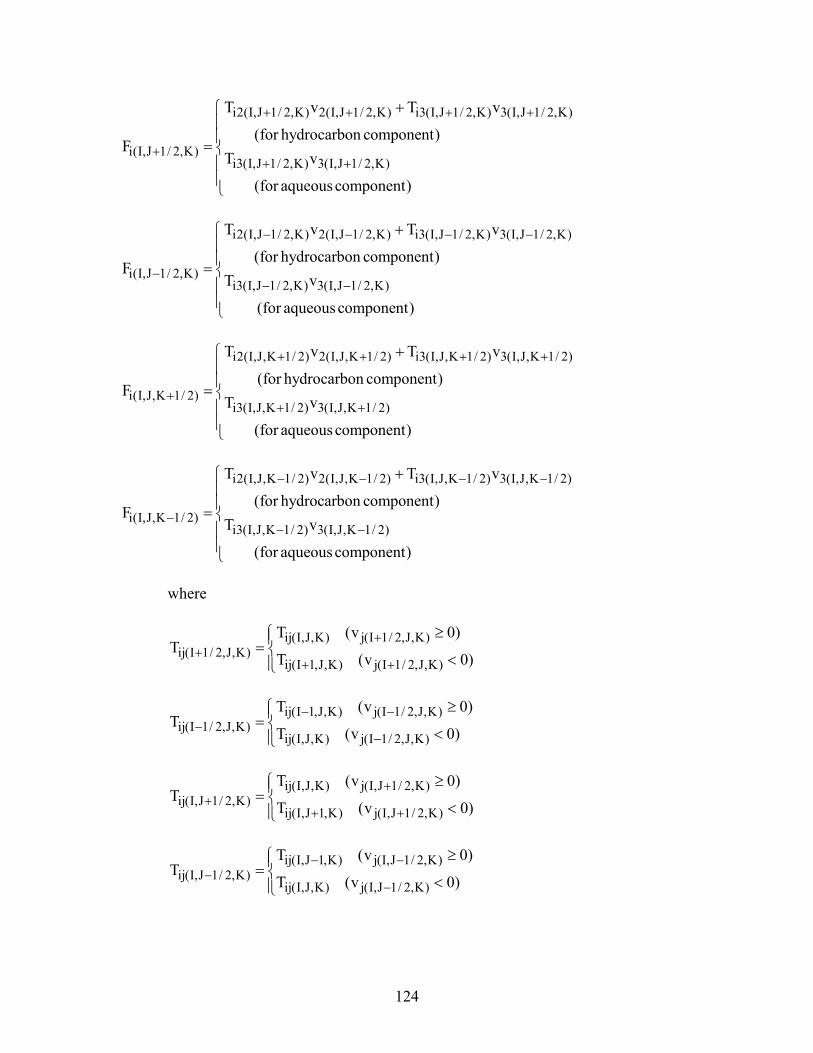
124
i2(I,J 1/ 2,K) 2(I,J 1/ 2,K) i3(I,J 1/ 2,K) 3(I,J 1/ 2,K)
i(I,J 1/ 2,K)i3(I,J 1/ 2,K) 3(I,J 1/ 2,K)
T v T v
(for hydrocarbon component)F
T v
(for aqueous component)
+ + + +
++ +
+=
i2(I,J 1/ 2,K) 2(I,J 1/ 2,K) i3(I,J 1/ 2,K) 3(I,J 1/ 2,K)
i(I,J 1/ 2,K)i3(I,J 1/ 2,K) 3(I,J 1/ 2,K)
T v T v
(for hydrocarbon component)F
T v
(for aqueous component)
− − − −
−− −
+=
i2(I,J,K 1/ 2) 2(I,J,K 1/ 2) i3(I,J,K 1/ 2) 3(I,J,K 1/ 2)
i(I,J,K 1/ 2)i3(I,J,K 1/ 2) 3(I,J,K 1/ 2)
T v T v
(for hydrocarbon component)F
T v
(for aqueous component)
+ + + +
++ +
+=
i2(I,J,K 1/ 2) 2(I,J,K 1/ 2) i3(I,J,K 1/ 2) 3(I,J,K 1/ 2)
i(I,J,K 1/ 2)i3(I,J,K 1/ 2) 3(I,J,K 1/ 2)
T v T v
(for hydrocarbon component)F
T v
(for aqueous component)
− − − −
−− −
+=
where
ij(I,J,K) j(I 1/ 2,J,K)
ij(I 1/ 2,J,K)ij(I 1,J,K) j(I 1/ 2,J,K)
T (v 0)T
T (v 0)+
++ +
≥= <
ij(I 1,J,K) j(I 1/ 2,J,K)
ij(I 1/ 2,J,K)ij(I,J,K) j(I 1/ 2,J,K)
T (v 0)T
T (v 0)− −
−−
≥= <
ij(I,J,K) j(I,J 1/ 2,K)
ij(I,J 1/ 2,K)ij(I,J 1,K) j(I,J 1/ 2,K)
T (v 0)T
T (v 0)+
++ +
≥= <
ij(I,J 1,K) j(I,J 1/ 2,K)
ij(I,J 1/ 2,K)ij(I,J,K) j(I,J 1/ 2,K)
T (v 0)T
T (v 0)− −
−−
≥= <
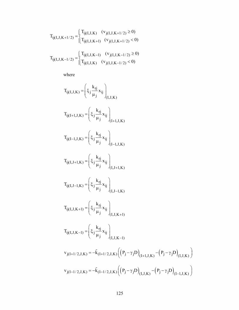
125
ij(I,J,K) j(I,J,K 1/ 2)
ij(I,J,K 1/ 2)ij(I,J,K 1) j(I,J,K 1/ 2)
T (v 0)T
T (v 0)+
++ +
≥= <
ij(I,J,K 1) j(I,J,K 1/ 2)
ij(I,J,K 1/ 2)ij(I,J,K) j(I,J,K 1/ 2)
T (v 0)T
T (v 0)− −
−−
≥= <
where
rjij(I,J,K) j ij
j (I,J,K)
kT x
= ξ µ
rjij(I 1,J,K) j ij
j (I 1,J,K)
kT x+
+
= ξ µ
rjij(I 1,J,K) j ij
j (I 1,J,K)
kT x−
−
= ξ µ
rjij(I,J 1,K) j ij
j (I,J 1,K)
kT x+
+
= ξ µ
rjij(I,J 1,K) j ij
j (I,J 1,K)
kT x−
−
= ξ µ
rjij(I,J,K 1) j ij
j (I,J,K 1)
kT x+
+
= ξ µ
rjij(I,J,K 1) j ij
j (I,J,K 1)
kT x−
−
= ξ µ
( ) ( )j(I 1/ 2,J,K) (I 1/ 2,J,K) j j j j(I 1,J,K) (I,J,K)v k P D P D+ + +
= − − γ − − γ
( ) ( )j(I 1/ 2,J,K) (I 1/ 2,J,K) j j j j(I,J,K) (I 1,J,K)v k P D P D− − −
= − − γ − − γ
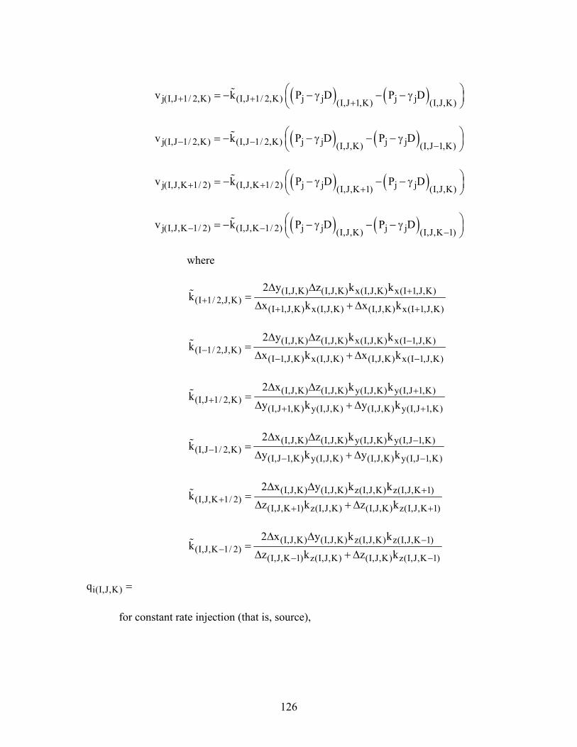
126
( ) ( )j(I,J 1/ 2,K) (I,J 1/ 2,K) j j j j(I,J 1,K) (I,J,K)v k P D P D+ + +
= − − γ − − γ
( ) ( )j(I,J 1/ 2,K) (I,J 1/ 2,K) j j j j(I,J,K) (I,J 1,K)v k P D P D− − −
= − − γ − − γ
( ) ( )j(I,J,K 1/ 2) (I,J,K 1/ 2) j j j j(I,J,K 1) (I,J,K)v k P D P D+ + +
= − − γ − − γ
( ) ( )j(I,J,K 1/ 2) (I,J,K 1/ 2) j j j j(I,J,K) (I,J,K 1)v k P D P D− − −
= − − γ − − γ
where
(I,J,K) (I,J,K) x(I,J,K) x(I 1,J,K)(I 1/ 2,J,K)
(I 1,J,K) x(I,J,K) (I,J,K) x(I 1,J,K)
2 y z k kk
x k x k+
++ +
∆ ∆=
∆ + ∆
(I,J,K) (I,J,K) x(I,J,K) x(I 1,J,K)(I 1/ 2,J,K)
(I 1,J,K) x(I,J,K) (I,J,K) x(I 1,J,K)
2 y z k kk
x k x k−
−− −
∆ ∆=
∆ + ∆
(I,J,K) (I,J,K) y(I,J,K) y(I,J 1,K)(I,J 1/ 2,K)
(I,J 1,K) y(I,J,K) (I,J,K) y(I,J 1,K)
2 x z k kk
y k y k+
++ +
∆ ∆=
∆ + ∆
(I,J,K) (I,J,K) y(I,J,K) y(I,J 1,K)(I,J 1/ 2,K)
(I,J 1,K) y(I,J,K) (I,J,K) y(I,J 1,K)
2 x z k kk
y k y k−
−− −
∆ ∆=
∆ + ∆
(I,J,K) (I,J,K) z(I,J,K) z(I,J,K 1)(I,J,K 1/ 2)
(I,J,K 1) z(I,J,K) (I,J,K) z(I,J,K 1)
2 x y k kk
z k z k+
++ +
∆ ∆=
∆ + ∆
(I,J,K) (I,J,K) z(I,J,K) z(I,J,K 1)(I,J,K 1/ 2)
(I,J,K 1) z(I,J,K) (I,J,K) z(I,J,K 1)
2 x y k kk
z k z k−
−− −
∆ ∆=
∆ + ∆
i(I,J,K)q =
for constant rate injection (that is, source),
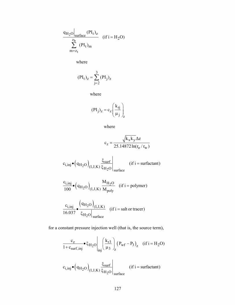
127
2
b
t
H O t zsurface2z
t mm z
q (PI )(if i H O)
(PI )=
=
∑
where
3
t z j zj 2
(PI ) (PI )=
= ∑
where
rjj z z
j z
k(PI ) c
= µ
where
x yz
o w
k k zc
25.14872ln(r / r )
∆=
( )22
surfi,inj H O (I,J,K) H O surface
c q (if i surfactant)ξ
• =ξ
( ) 22
H Oi,injH O (I,J,K) poly
Mcq (if i polymer)
100 M• =
( )2
2
H Oi,inj (I,J,K)
H O surface
qc(if i salt or tracer)
16.037• =
ξ
for a constant pressure injection well (that is, the source term),
( )2r3z
H O wf 3 2zsurf ,inj 3 zinj
kc P P (if i H O)1 c
• ξ − = + µ
( )22
surfi,inj H O (I,J,K) H O surface
c q (if i surfactant)ξ
• =ξ
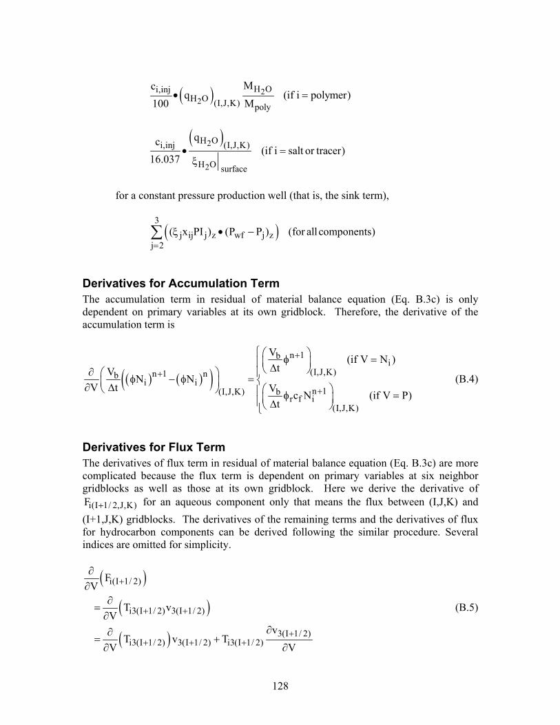
128
( ) 22
H Oi,injH O (I,J,K) poly
Mcq (if i polymer)
100 M• =
( )2
2
H Oi,inj (I,J,K)
H O surface
qc(if i salt or tracer)
16.037• =
ξ
for a constant pressure production well (that is, the sink term),
( )3
j ij j z wf j zj 2
( x PI ) (P P ) (for all components)=
ξ • −∑
Derivatives for Accumulation Term The accumulation term in residual of material balance equation (Eq. B.3c) is only dependent on primary variables at its own gridblock. Therefore, the derivative of the accumulation term is
( ) ( )( )n 1b
i(I,J,K)n 1 nb
i in 1(I,J,K) b
r f i(I,J,K)
V (if V N )tV
N NV t V c N (if V P)
t
+
+
+
φ = ∆ ∂ φ − φ = ∂ ∆ φ = ∆
(B.4)
Derivatives for Flux Term The derivatives of flux term in residual of material balance equation (Eq. B.3c) are more complicated because the flux term is dependent on primary variables at six neighbor gridblocks as well as those at its own gridblock. Here we derive the derivative of
i(I 1/ 2,J,K)F + for an aqueous component only that means the flux between (I,J,K) and (I+1,J,K) gridblocks. The derivatives of the remaining terms and the derivatives of flux for hydrocarbon components can be derived following the similar procedure. Several indices are omitted for simplicity.
( )
( )
( )
i(I 1/ 2)
i3(I 1/ 2) 3(I 1/ 2)
3(I 1/ 2)i3(I 1/ 2) 3(I 1/ 2) i3(I 1/ 2)
FV
T vV
vT v T
V V
+
+ +
++ + +
∂∂
∂=
∂∂∂
= +∂ ∂
(B.5)
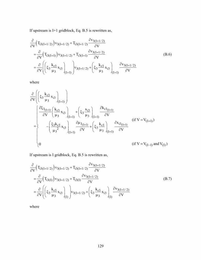
129
If upstream is I+1 gridblock, Eq. B.5 is rewritten as,
( )
( )
3(I 1/ 2)i3(I 1/ 2) 3(I 1/ 2) i3(I 1/ 2)
3(I 1/ 2)i3(I 1) 3(I 1/ 2) i3(I 1)
3(I 1/ 2)r3 r33 i3 3(I 1/ 2) 3 i3
3 3(I 1) (I 1)
vT v T
V Vv
T v TV V
vk kx v x
V V
++ + +
++ + +
++
+ +
∂∂+
∂ ∂∂∂
= +∂ ∂
∂ ∂ = ξ + ξ ∂ µ µ ∂
(B.6)
where
(I 1) (I 1)
(I 1) (I 1)
r33 i3
3 (I 1)
3 r3r3 i3i3 3
3 3(I 1) (I 1)(I 1)
3 i33 r3 r3i3 32 33 (I 1)(I 1)
(I 1) (I)
k xV
kk xxV V
(if V V )xk kx
V V
(if V V and V )0
+ +
+ +
+
+ ++
++
−
∂ ξ ∂ µ ∂ξ ∂
+ ξ ∂ µ µ ∂ =
∂µ ∂ ξ= − + ξ ∂ µ ∂µ =
If upstream is I gridblock, Eq. B.5 is rewritten as,
( )
( )
3(I 1/ 2)i3(I 1/ 2) 3(I 1/ 2) i3(I 1/ 2)
3(I 1/ 2)i3(I) 3(I 1/ 2) i3(I)
3(I 1/ 2)r3 r33 i3 3(I 1/ 2) 3 i3
3 3(I) (I)
vT v T
V Vv
T v TV V
vk kx v x
V V
++ + +
++
++
∂∂+
∂ ∂∂∂
= +∂ ∂
∂ ∂ = ξ + ξ ∂ µ µ ∂
(B.7)
where
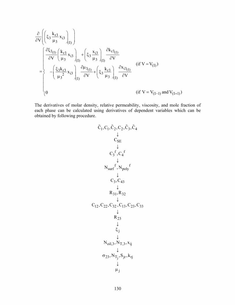
130
(I) (I)
(I) (I)
r33 i3
3 (I)
3 r3r3 i3i3 3
3 3(I) (I)(I)
3 i33 r3 r3i3 32 33 (I)(I)
(I 1) (I 1)
k xV
kk xxV V
(if V V )xk kx
V V
(if V V and V )0 − +
∂ ξ ∂ µ ∂ξ ∂
+ ξ ∂ µ µ ∂ =
∂µ ∂ ξ= − + ξ ∂ µ ∂µ =
The derivatives of molar density, relative permeability, viscosity, and mole fraction of each phase can be calculated using derivatives of dependent variables which can be obtained by following procedure.
1 1 2 2 3 4C ,C ,C ,C ,C ,C ↓ SEC ↓
f f3 4C ,C ↓
f fsurf polyN , N
↓ 3 43C ,C ↓
31 32R ,R ↓
12 22 32C ,C ,C , 13 23 33C ,C ,C ↓ 23R ↓
jξ ↓
oil,3 T,3 ijN , N , x ↓
j23 T jr rj, N ,S ,kσ
↓ jµ
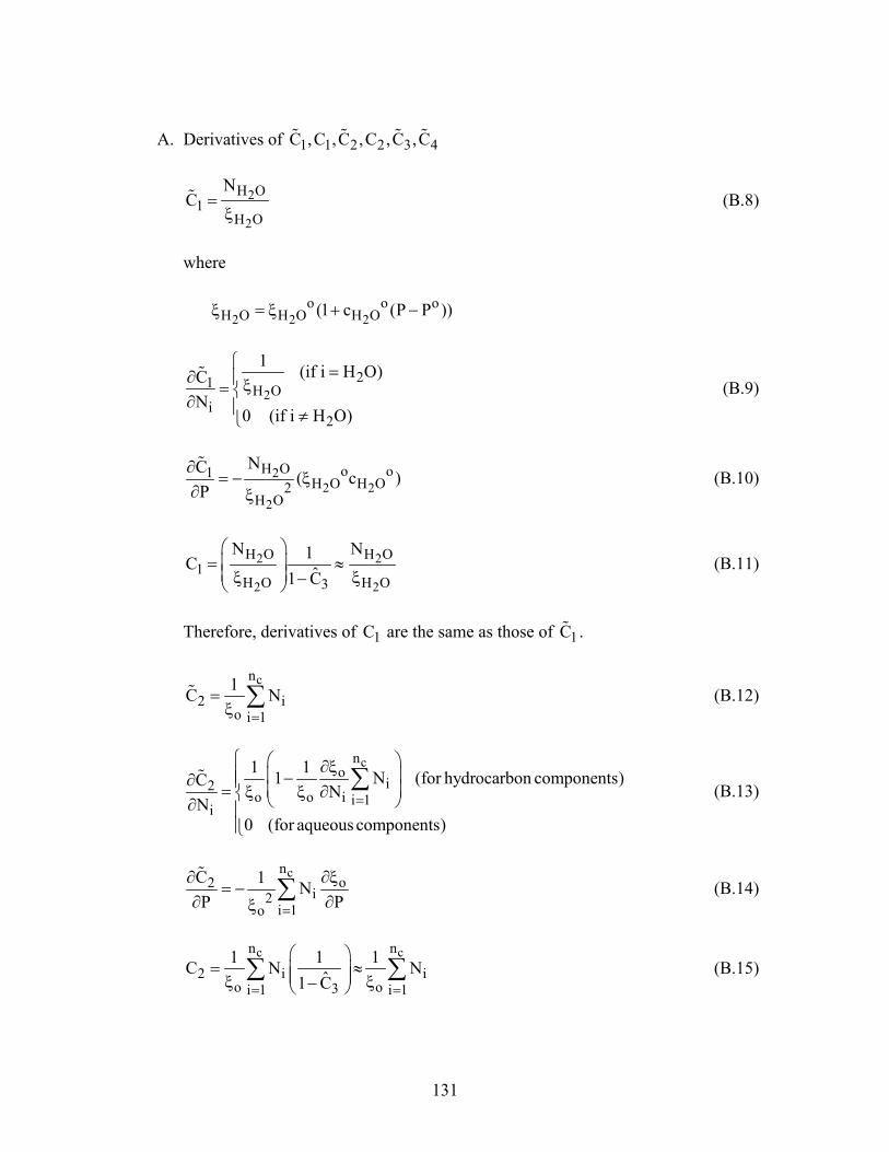
131
A. Derivatives of 1 1 2 2 3 4C ,C ,C ,C ,C ,C
2
2
H O1
H O
NC =
ξ (B.8)
where
2 2 2o o o
H O H O H O(1 c (P P ))ξ = ξ + −
221 H O
i2
1 (if i H O)CN
0 (if i H O)
=∂ ξ= ∂ ≠
(B.9)
22 2
2
H O o o1H O H O2
H O
NC ( c )P
∂= − ξ
∂ ξ (B.10)
2 2
2 2
H O H O1
H O H O3
N N1C ˆ1 C
= ≈ ξ ξ−
(B.11)
Therefore, derivatives of 1C are the same as those of 1C .
cn
2 io i 1
1C N=
=ξ ∑ (B.12)
cno
i2o o i i 1
i
1 11 N (for hydrocarbon components)CN
N0 (for aqueous components)
=
∂ξ −∂ = ξ ξ ∂ ∂
∑ (B.13)
cn
o2i2
i 1o
C 1 NP P=
∂ξ∂= −
∂ ∂ξ∑ (B.14)
c cn n
2 i io o3i 1 i 1
1 1 1C N Nˆ1 C= =
= ≈ ξ ξ−
∑ ∑ (B.15)
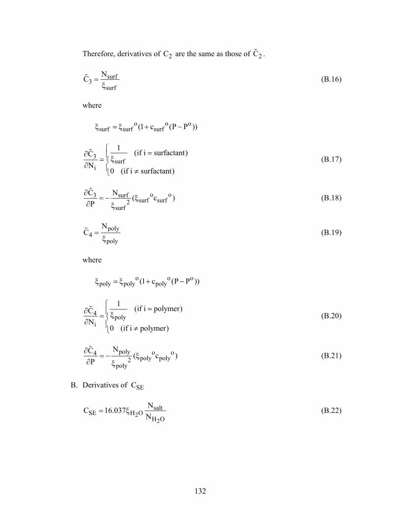
132
Therefore, derivatives of 2C are the same as those of 2C .
surf3
surf
NC =ξ
(B.16)
where
o o osurf surf surf(1 c (P P ))ξ = ξ + −
3surf
i
1 (if i surfactant)CN
0 (if i surfactant)
=∂ ξ= ∂ ≠
(B.17)
o o3 surfsurf surf2
surf
C N ( c )P
∂= − ξ
∂ ξ (B.18)
poly4
poly
NC =
ξ (B.19)
where
o o opoly poly poly(1 c (P P ))ξ = ξ + −
4 polyi
1 (if i polymer)CN
0 (if i polymer)
=∂ ξ= ∂ ≠
(B.20)
poly o o4poly poly2
poly
NC ( c )P
∂= − ξ
∂ ξ (B.21)
B. Derivatives of SEC
22
saltSE H O
H O
NC 16.037N
= ξ (B.22)
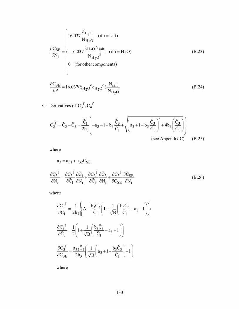
133
2
2
2
2
H O
H O
H O saltSE22i H O
16.037 (if i salt)N
NC16.037 (if i H O)
N N
0 (for other components)
ξ=
ξ∂ = − =∂
(B.23)
2 22
o oSE saltH O H O
H O
C N16.037( c )P N
∂= ξ
∂ (B.24)
C. Derivatives of f f
3 4C ,C
2
f 3 3 313 3 3 3 3 3 3 3
3 1 1 1
C C CCˆC C C a 1 b a 1 b 4b2b C C C
= − = − − + + + − +
(see Appendix C) (B.25) where
3 31 32 SEa a a C= +
f f f f
3 3 3 3 3 SE1
i i i SE i1 3
C C C C C CCN N N C NC C
∂ ∂ ∂ ∂ ∂ ∂∂= + +
∂ ∂ ∂ ∂ ∂∂ ∂ (B.26)
where
f
3 3 3 3 33
31 1 1
C b C b C1 1A 1 a 12bC C CB
∂ = − − − − ∂
f
3 3 33
3 1
C b C1 11 a 12C CB
∂= + − + ∂
f
3 32 1 3 33
SE 3 1
C a C b C1 a 1 1C 2b CB
∂= + − − ∂
where
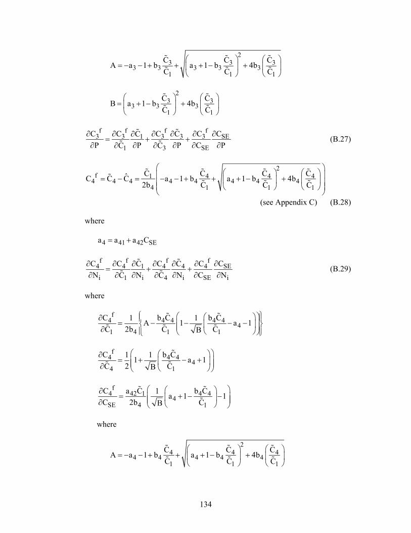
134
2
3 3 33 3 3 3 3
1 1 1
C C CA a 1 b a 1 b 4bC C C
= − − + + + − +
2
3 33 3 3
1 1
C CB a 1 b 4bC C
= + − +
f f f f
3 3 3 3 3 SE1
SE1 3
C C C C C CCP P P C PC C
∂ ∂ ∂ ∂ ∂ ∂∂= + +
∂ ∂ ∂ ∂ ∂∂ ∂ (B.27)
2
f 1 4 4 44 4 4 4 4 4 4 4
4 1 1 1
C C C CˆC C C a 1 b a 1 b 4b2b C C C
= − = − − + + + − +
(see Appendix C) (B.28) where
4 41 42 SEa a a C= +
f f f f
SE4 4 1 4 4 4
i i i SE i1 4
CC C C C C CN N N C NC C
∂∂ ∂ ∂ ∂ ∂ ∂= + +
∂ ∂ ∂ ∂ ∂∂ ∂ (B.29)
where
f
4 4 4 4 44
41 1 1
C b C b C1 1A 1 a 12bC C CB
∂ = − − − − ∂
f
4 4 44
4 1
C b C1 11 a 12C CB
∂= + − + ∂
f
4 42 1 4 44
SE 4 1
C a C b C1 a 1 1C 2b CB
∂= + − − ∂
where
2
4 4 44 4 4 4 4
1 1 1
C C CA a 1 b a 1 b 4bC C C
= − − + + + − +
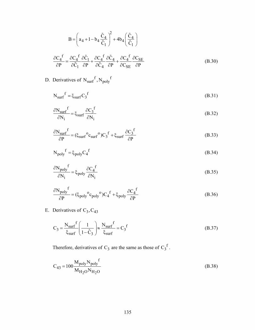
135
2
4 44 4 4
1 1
C CB a 1 b 4bC C
= + − +
f f f f
SE4 4 1 4 4 4
SE1 4
CC C C C C CP P P C PC C
∂∂ ∂ ∂ ∂ ∂ ∂= + +
∂ ∂ ∂ ∂ ∂∂ ∂ (B.30)
D. Derivatives of f f
surf polyN , N f f
surf surf 3N C= ξ (B.31)
f f
surf 3surf
i i
N CN N
∂ ∂= ξ
∂ ∂ (B.32)
f f
o o fsurf 3surf surf 3 surf
N C( c )CP P
∂ ∂= ξ + ξ
∂ ∂ (B.33)
f f
poly poly 4N C= ξ (B.34)
f fpoly 4
polyi i
N CN N
∂ ∂= ξ
∂ ∂ (B.35)
f fpoly o o f 4
poly poly 4 polyN C( c )C
P P∂ ∂
= ξ + ξ∂ ∂
(B.36)
E. Derivatives of 3 43C ,C
f f
fsurf surf3 3
surf surf3
N N1C Cˆ1 C
= ≈ = ξ ξ−
(B.37)
Therefore, derivatives of 3C are the same as those of f
3C .
2 2
fpoly poly
43H O H O
M NC 100
M N= (B.38)
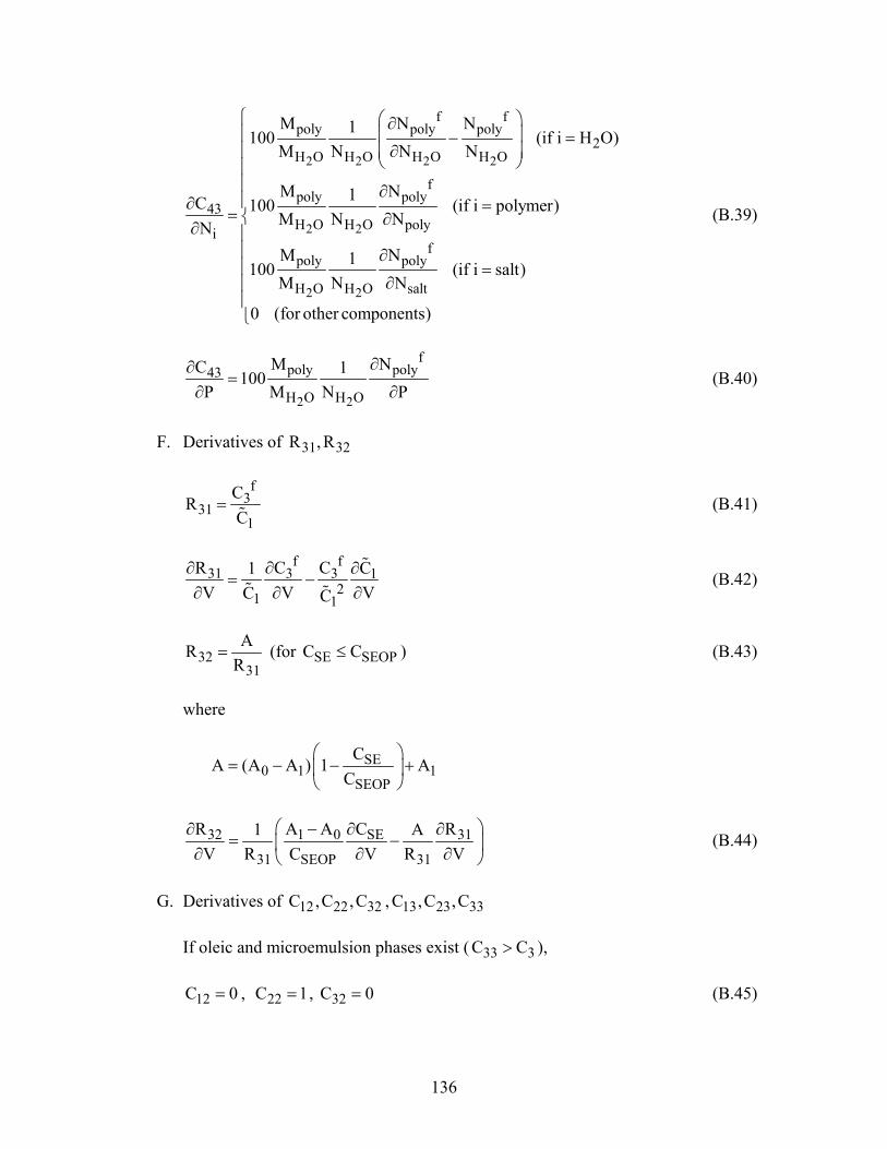
136
2 2 2 2
2 2
2 2
f fpoly poly poly
2H O H O H O H O
fpoly poly
43H O H O polyi
fpoly poly
H O H O salt
M N N1100 (if i H O)M N N N
M N1C 100 (if i polymer)M N NNM N1100 (if i salt)M N N
0 (for other components)
∂ − = ∂
∂∂ == ∂∂ ∂ =
∂
(B.39)
2 2
fpoly poly43
H O H O
M NC 1100P M N P
∂∂=
∂ ∂ (B.40)
F. Derivatives of 31 32R ,R
f
331
1
CRC
= (B.41)
f f
31 3 3 12
1 1
R C C C1V V VC C
∂ ∂ ∂= −
∂ ∂ ∂ (B.42)
3231
ARR
= (for SE SEOPC C≤ ) (B.43)
where
SE0 1 1
SEOP
CA (A A ) 1 A
C
= − − +
32 1 0 SE 31
31 SEOP 31
R A A C R1 AV R C V R V
∂ − ∂ ∂= − ∂ ∂ ∂
(B.44)
G. Derivatives of 12 22 32C ,C ,C , 13 23 33C ,C ,C If oleic and microemulsion phases exist ( 33 3C C> ), 12C 0= , 22C 1= , 32C 0= (B.45)
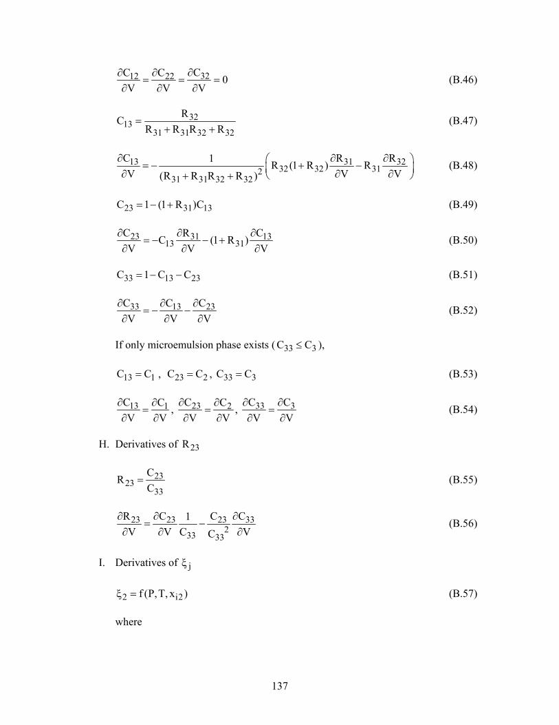
137
3212 22 CC C 0V V V
∂∂ ∂= = =
∂ ∂ ∂ (B.46)
3213
31 31 32 32
RCR R R R
=+ +
(B.47)
13 31 3232 32 312
31 31 32 32
C R R1 R (1 R ) RV V V(R R R R )
∂ ∂ ∂ = − + − ∂ ∂ ∂ + + (B.48)
23 31 13C 1 (1 R )C= − + (B.49)
23 31 1313 31
C R CC (1 R )V V V
∂ ∂ ∂= − − +
∂ ∂ ∂ (B.50)
33 13 23C 1 C C= − − (B.51)
33 13 23C C CV V V
∂ ∂ ∂= − −
∂ ∂ ∂ (B.52)
If only microemulsion phase exists ( 33 3C C≤ ), 13 1C C= , 23 2C C= , 33 3C C= (B.53)
13 1C CV V
∂ ∂=
∂ ∂, 23 2C C
V V∂ ∂
=∂ ∂
, 33 3C CV V
∂ ∂=
∂ ∂ (B.54)
H. Derivatives of 23R
2323
33
CRC
= (B.55)
23 23 23 33233 33
R C C C1V V C VC
∂ ∂ ∂= −
∂ ∂ ∂ (B.56)
I. Derivatives of jξ 2 i2f (P,T, x )ξ = (B.57) where
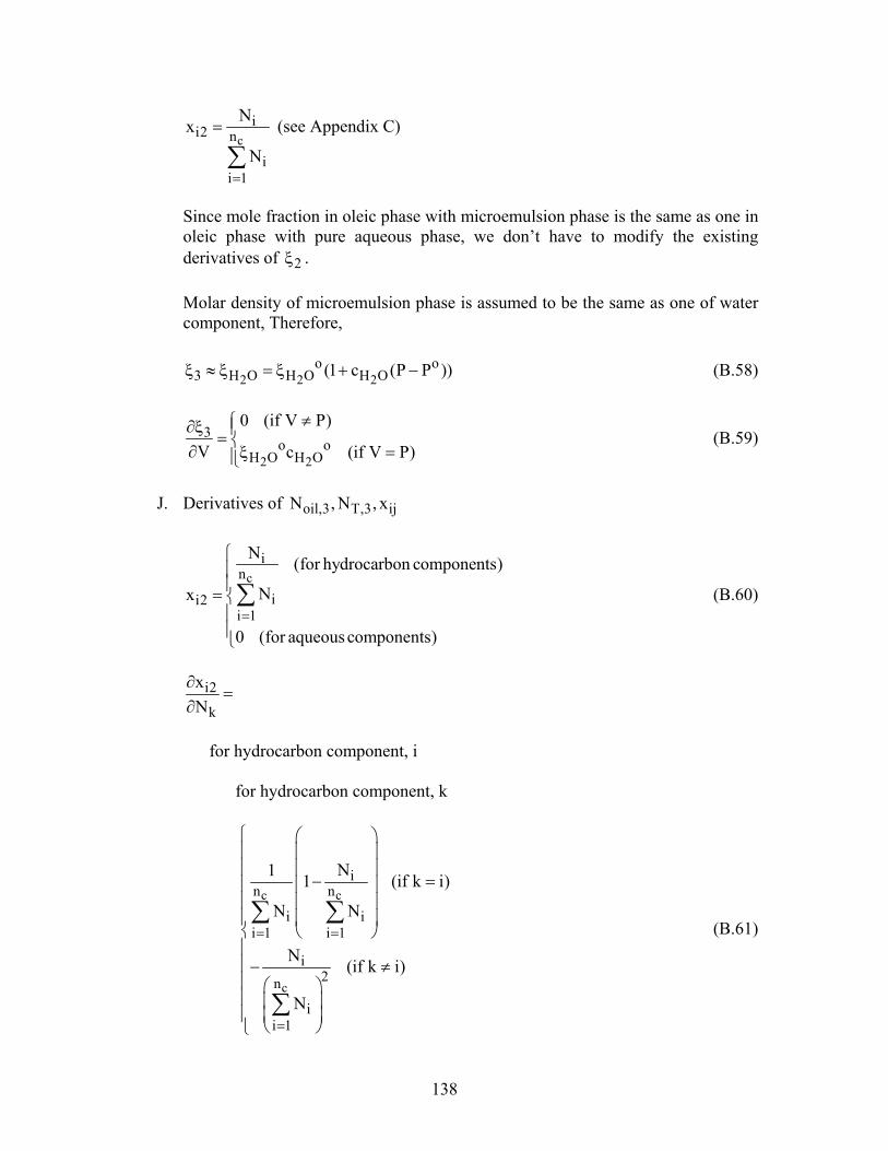
138
ci
i2 n
ii 1
Nx
N=
=
∑ (see Appendix C)
Since mole fraction in oleic phase with microemulsion phase is the same as one in
oleic phase with pure aqueous phase, we don’t have to modify the existing derivatives of 2ξ .
Molar density of microemulsion phase is assumed to be the same as one of water
component, Therefore, 2 2 2
o o3 H O H O H O(1 c (P P ))ξ ≈ ξ = ξ + − (B.58)
2 2
3o o
H O H O
0 (if V P)
V c (if V P)
≠∂ξ = ∂ ξ = (B.59)
J. Derivatives of oil,3 T,3 ijN , N , x
c
in
ii2i 1
N (for hydrocarbon components)
Nx
0 (for aqueous components)=
=
∑ (B.60)
i2
k
xN
∂=
∂
for hydrocarbon component, i
for hydrocarbon component, k
c c
c
in n
i ii 1 i 1
i2n
ii 1
N1 1 (if k i)
N N
N (if k i)
N
= =
=
− = − ≠
∑ ∑
∑
(B.61)
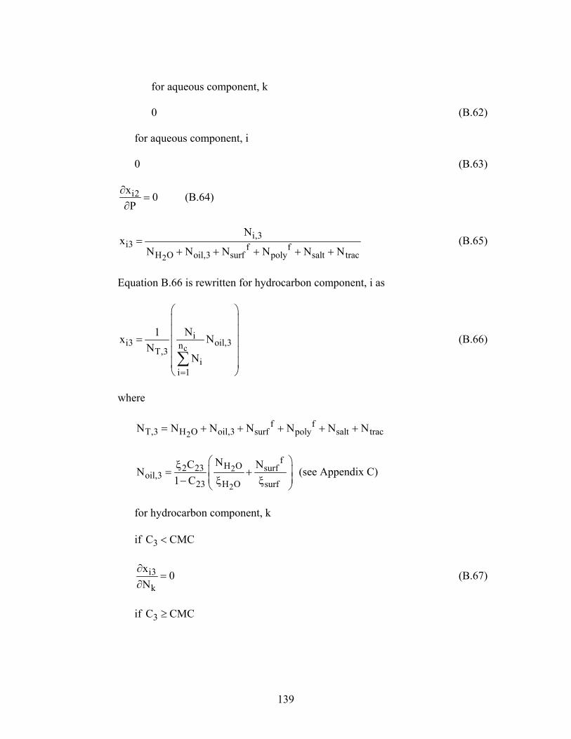
139
for aqueous component, k 0 (B.62)
for aqueous component, i 0 (B.63)
i2x 0P
∂=
∂ (B.64)
2
i,3i3 f f
H O oil,3 surf poly salt trac
Nx
N N N N N N=
+ + + + + (B.65)
Equation B.66 is rewritten for hydrocarbon component, i as
c
ii3 oil,3nT,3
ii 1
N1x NN
N=
= ∑
(B.66)
where
2f f
T,3 H O oil,3 surf poly salt tracN N N N N N N= + + + + +
2
2
fH O2 23 surfoil,3
23 H O surf
NC NN
1 C
ξ = + − ξ ξ
(see Appendix C)
for hydrocarbon component, k if 3C CMC<
i3
k
x 0N
∂=
∂ (B.67)
if 3C CMC≥
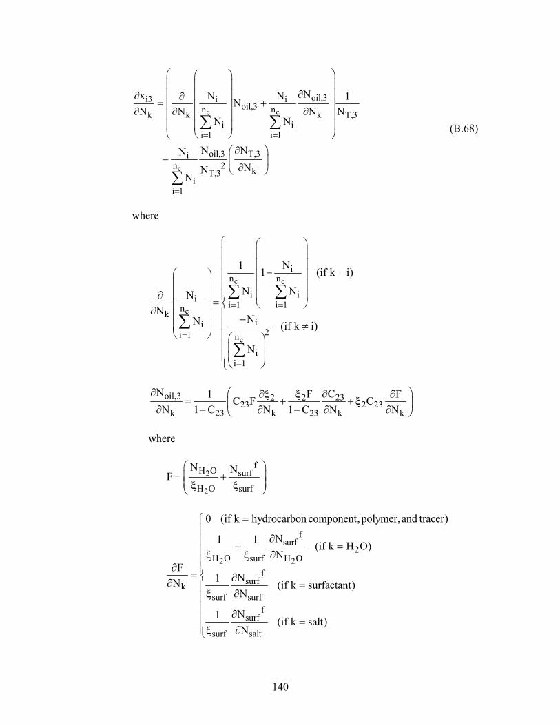
140
c c
c
oil,3i3 i ioil,3n nk k k T,3
i ii 1 i 1
oil,3 T,3in 2 kT,3
ii 1
Nx N N 1NN N N N
N N
N NNNN
N
= =
=
∂ ∂ ∂= + ∂ ∂ ∂
∂ − ∂
∑ ∑
∑
(B.68)
where
c c
c
c
in n
i iii 1 i 1nk
ii2i 1 n
ii 1
N1 1 (if k i)
N NNN
NN (if k i)
N
= =
=
=
− = ∂ = ∂ − ≠
∑ ∑
∑
∑
oil,3 232 223 2 23
k 23 k 23 k k
N CF1 FC F CN 1 C N 1 C N N
∂ ∂∂ξ ξ ∂= + + ξ ∂ − ∂ − ∂ ∂
where
2
2
fH O surf
H O surf
N NF
= + ξ ξ
2 2
fsurf
2H O surf H O
fsurfk
surf surff
surf
surf salt
0 (if k hydrocarbon component, polymer,and tracer)
N1 1 (if k H O)N
FN1N (if k surfactant)N
N1 (if k salt)N
=
∂ + =ξ ξ ∂∂ = ∂∂ =ξ ∂ ∂ =ξ ∂
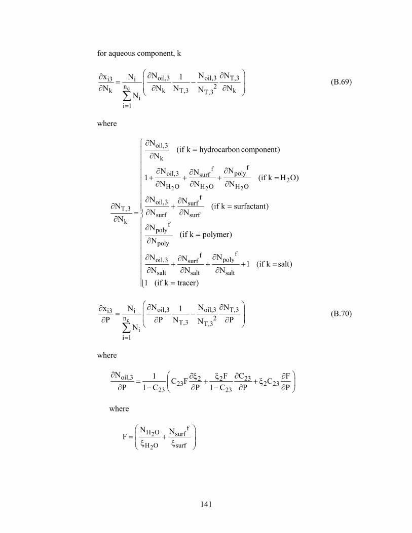
141
for aqueous component, k
c
oil,3 oil,3 T,3i3 in 2k k T,3 kT,3
ii 1
N N Nx N 1N N N NN
N=
∂ ∂∂ = − ∂ ∂ ∂ ∑
(B.69)
where
2 2 2
oil,3
kff polyoil,3 surf
2H O H O H O
foil,3 surf
T,3surf surf
k fpoly
polyff polyoil,3 surf
salt salt
N(if k hydrocarbon component)
N
NN N1 (if k H O)
N N N
N NN (if k surfactant)
N NN
N(if k polymer)
N
NN NN N N
∂=
∂
∂∂ ∂+ + + =
∂ ∂ ∂
∂ ∂∂ + =
∂ ∂=∂
∂=
∂
∂∂ ∂+ +
∂ ∂ ∂ salt1 (if k salt)
1 (if k tracer)
+ =
=
c
oil,3 oil,3 T,3i3 in 2T,3 T,3
ii 1
N N Nx N 1P P N PN
N=
∂ ∂∂ = − ∂ ∂ ∂ ∑
(B.70)
where
oil,3 232 223 2 23
23 23
N CF1 FC F CP 1 C P 1 C P P
∂ ∂∂ξ ξ ∂= + + ξ ∂ − ∂ − ∂ ∂
where
2
2
fH O surf
H O surf
N NF
= + ξ ξ
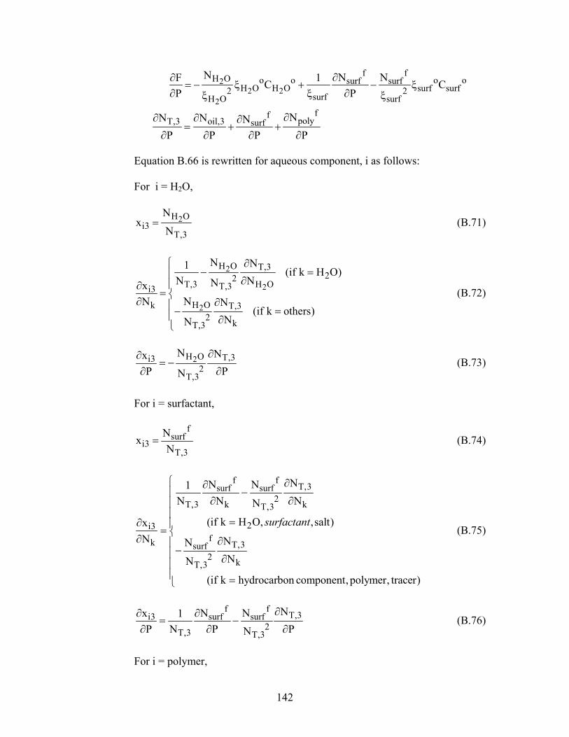
142
22 2
2
f fH O o o o osurf surfH O H O surf surf2 2surfH O surf
N N NF 1C CP P
∂∂= − ξ + − ξ
∂ ξ ∂ξ ξ
ff polyT,3 oil,3 surf NN N N
P P P P∂∂ ∂ ∂
= + +∂ ∂ ∂ ∂
Equation B.66 is rewritten for aqueous component, i as follows: For i = H2O,
2H Oi3
T,3
Nx
N= (B.71)
2
2
2
H O T,322T,3 H OT,3i3
H Ok T,32 kT,3
N N1 (if k H O)N NNx
NN N(if k others)
NN
∂− = ∂∂
= ∂ ∂− = ∂
(B.72)
2H O T,3i32
T,3
N NxP PN
∂∂= −
∂ ∂ (B.73)
For i = surfactant,
f
surfi3
T,3
NxN
= (B.74)
f fT,3surf surf
2T,3 k kT,3
2i3fk T,3surf2 kT,3
NN N1N N NN
(if k H O, ,salt)xN NN
NN
(if k hydrocarbon component, polymer, tracer)
∂∂−
∂ ∂
=∂ = ∂ ∂− ∂
=
surfactant (B.75)
f f
T,3i3 surf surf2T,3 T,3
Nx N N1P N P PN
∂∂ ∂= −
∂ ∂ ∂ (B.76)
For i = polymer,
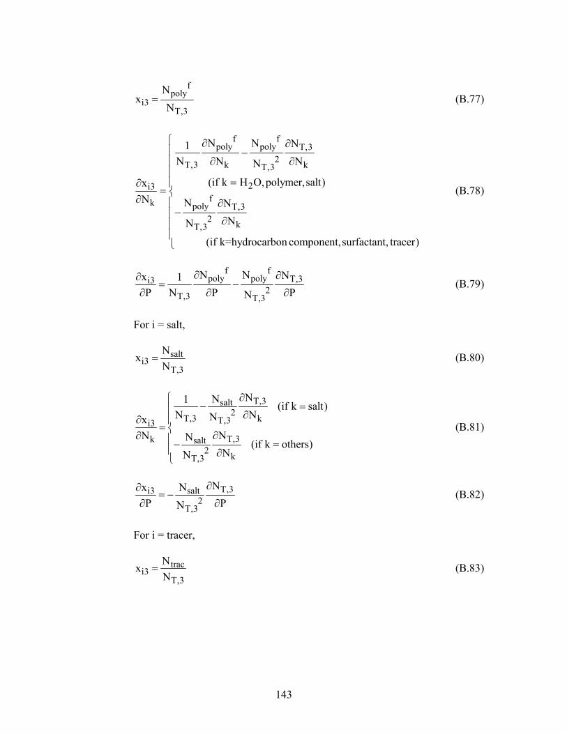
143
f
polyi3
T,3
Nx
N= (B.77)
f fpoly poly T,3
2T,3 k kT,3
2i3fk poly T,32 kT,3
N N N1N N NN
(if k H O,polymer,salt)xN N N
NN
(if k=hydrocarbon component,surfactant, tracer)
∂ ∂ −
∂ ∂
=∂ = ∂ ∂
−∂
(B.78)
f f
poly poly T,3i32T,3 T,3
N N Nx 1P N P PN
∂ ∂∂= −
∂ ∂ ∂ (B.79)
For i = salt,
salti3
T,3
NxN
= (B.80)
T,3salt2T,3 kT,3i3
T,3k salt2 kT,3
NN1 (if k salt)N NNx
NN N (if k others)NN
∂− = ∂∂
= ∂∂ − = ∂
(B.81)
T,3i3 salt2
T,3
Nx NP PN
∂∂= −
∂ ∂ (B.82)
For i = tracer,
traci3
T,3
NxN
= (B.83)
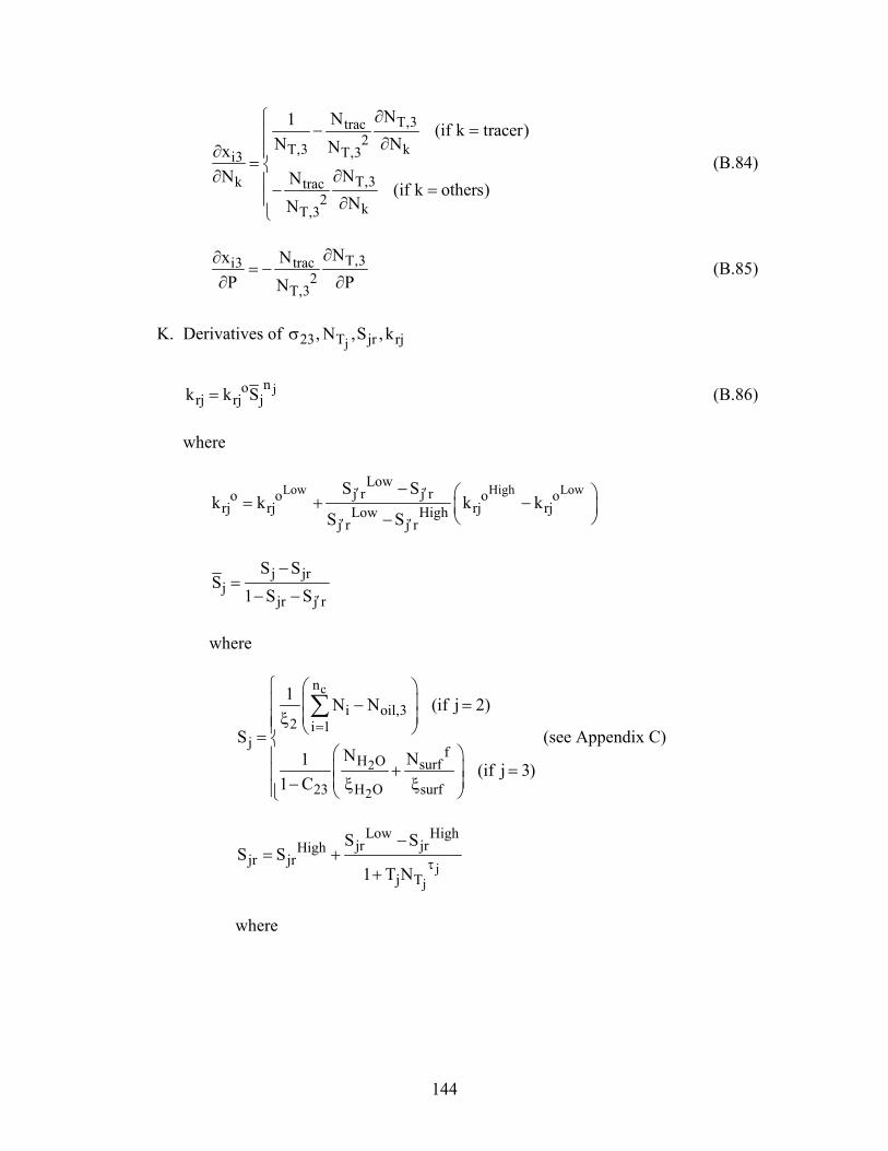
144
T,3trac2T,3 kT,3i3
T,3k trac2 kT,3
NN1 (if k tracer)N NNx
NN N (if k others)NN
∂− = ∂∂
= ∂∂ − = ∂
(B.84)
T,3i3 trac2
T,3
Nx NP PN
∂∂= −
∂ ∂ (B.85)
K. Derivatives of j23 T jr rj, N ,S ,kσ
jnorj rj jk k S= (B.86)
where
Low High LowLow
j r j ro o o orj rj rj rjLow High
j r j r
S Sk k k k
S S′ ′
′ ′
− = + − −
j jrj
jr j r
S SS
1 S S ′
−=
− −
where
c
2
2
n
i oil,32 i 1
jfH O surf
23 H O surf
1 N N (if j 2)
SN N1 (if j 3)
1 C
=
− =
ξ = + = − ξ ξ
∑ (see Appendix C)
j
j
Low Highjr jrHigh
jr jrj T
S SS S
1 T N τ
−= +
+
where
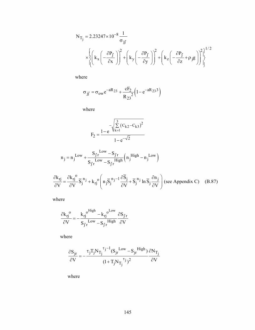
145
j8
Tjj
1/ 22 2 2j j j
x y z j
1N 2.23247 10
P P Pk k k g
x y z
−
′
′ ′ ′
= ×σ
∂ ∂ ∂ × − + − + − + ρ ∂ ∂ ∂
where
( )23 23aR aR 32jj ow 2
23
cFe 1 eR
− −′σ = σ + −
where
( )3 2
k2 k3k 1
C C
2 21 eF
1 e
=− −
−
∑−
=−
( )Low
j r j rLow High Lowj j j jLow High
j r j r
S Sn n n n
S S′ ′
′ ′
−= + −
−
j j jo
n n 1 nrj rj j joj rj j j j j
k k S nS k n S S ln S
V V V V− ∂ ∂ ∂ ∂
= + + ∂ ∂ ∂ ∂ (see Appendix C) (B.87)
where
High Lowo o o
rj rj rj j rLow High
j r j r
k k k SV VS S
′
′ ′
∂ − ∂= −
∂ ∂−
where
j
j j
jj
1 Low Highj j T jr jr Tjr
2j T
T N (S S ) NSV V(1 T N )
τ −
τ
τ − ∂∂= −
∂ ∂+
where
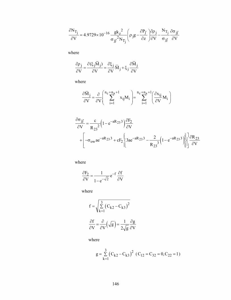
146
j j
j
2T Tj j jj16 zj2 jjjj T
N NPgk4.9729 10 gV z V VN
′ ′−
′′
∂ ∂ ∂ρ ∂σ = × ρ − − ∂ ∂ ∂ σ ∂σ
where
j j j j jj j
( M ) MM
V V V V∂ρ ∂ ξ ∂ξ ∂
= = + ξ∂ ∂ ∂ ∂
where
c a c an n 1 n n 1
j ijij i i
i 1 i 1
M xx M M
V V V
+ + + +
= =
∂ ∂ ∂ = = ∂ ∂ ∂ ∑ ∑
( )
( )
23
23 23 23
jj aR 3 22
23
aR aR aR3 3 3 23ow 2 3
23
Fc 1 eV VR
R2ae cF 3ae 1 eVR
′ −
− − −
∂σ ∂= −
∂ ∂
∂ + −σ + − − ∂
where
f22
F 1 feV V1 e
−−
∂ ∂=
∂ ∂−
where
( )3 2
k2 k3k 1
f C C=
= −∑
( )f 1 ggV V V2 g
∂ ∂ ∂= =
∂ ∂ ∂
where
( )3 2
k2 k3k 1
g C C=
= −∑ ( 12 32 22C C 0,C 1= = = )
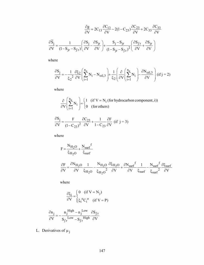
147
13 23 3313 23 33
C C Cg 2C 2(1 C ) 2CV V V V
∂ ∂ ∂∂= − − +
∂ ∂ ∂ ∂
j j jr j jr j r jr2jr j r jr j r
S S S S S S S1V (1 S S ) V V V V(1 S S )
′
′ ′
∂ ∂ ∂ − ∂ ∂ = − + + ∂ − − ∂ ∂ ∂ ∂− −
where
c cn n
j oil,32i oil,3 i2 2i 1 i 12
S N1 1N N NV V V V= =
∂ ∂∂ξ ∂ = − − + − ∂ ∂ ξ ∂ ∂ ξ ∑ ∑ (if j = 2)
where
cn
ii
i 1
1 (if V N (for hydrocarbon component, i))N
V 0 (for others)=
=∂ = ∂ ∑
j 232 2323
S CF 1 FV V 1 C V(1 C )
∂ ∂ ∂= +
∂ ∂ − ∂− (if j = 3)
where
2
2
fH O surf
H O surf
N NF = +ξ ξ
2 2 2
2 2
f fH O H O H O surf surf surf2 2H O surfH O surf
N N N NF 1 1V V V V V
∂ ∂ξ ∂ ∂ξ∂= − + −
∂ ∂ ξ ∂ ∂ ξ ∂ξ ξ
where
ji
o oi i
0 (if V N )
V C (if V P)
=∂ξ = ∂ ξ =
High Low
j j j j rLow High
j r j r
n n n SV VS S
′
′ ′
∂ − ∂= −
∂ ∂−
L. Derivatives of jµ
148
2 i2f (P,T, x )µ = (B.88) where
c
ii2 n
ii 1
Nx
N=
=
∑
1 23 33 2 13 33 4 13 5 23(C C ) (C C ) ( C C )
3 13 p 23 2 33 3C e C e C eα + α + α +αµ = µ + µ + α (B.89) where
( )( )pS2 3p w p1 43 p2 43 p3 43 SE1 A C A C A C Cµ = µ + + +
( )( )
1 23 33
1 23 33 2 33 2 13 5 23 4 13
1 23 33 2 13 33 4 13 5 23
1 23 33 2 13 33
p(C C )313
(C C ) ( C C ) ( C C ) 13p 23 2 2 33 3 4
(C C ) (C C ) ( C C ) 23p 13 1 2 33 3 5
(C C ) (C C ) (p 13 1 2 23 2 3
C eV V
Ce C e C eV
CC e e C eV
C e C e e
α +
α + α +α α +α
α + α + α +α
α + α + α
∂µ∂µ=
∂ ∂∂
+ µ + α µ + α α∂
∂+ µ α + µ + α α
∂
+ µ α + µ α + α( )4 13 5 23
2 13 33
C C ) 33
(C C ) 223
CV
C eV
+α
α +
∂∂
∂µ+
∂
(B.90)
where
( )( )
( )
p
p
S 1 2 43w SE SE p1 p2 43 p3 43
p 2 3 SEp p1 43 p2 43 p3 43
p
2 43w p1 p2 43 p3 43
if S 0
CC C A 2A C 3A C
VC
S A C A C A CV V
if S 0
CA 2A C 3A C
V
−
≠
∂ µ + + ∂∂µ ∂ = + + + ∂ ∂
=
∂µ + + ∂
Derivatives for Source/Sink Term For a constant rate injection,
149
For i = H2O,
2H O surfacei2
qq a(A a)V VA
∂ ∂= −
∂ ∂ (B.91)
where
b
t
z
t mm z
A (PI )=
= ∑
t za (PI )=
3 rj rj j
z 2jj 2 j
k ka 1cV V V=
∂ ∂µ∂ = − ∂ µ ∂ ∂µ
∑
For i = surfactant,
2
2
H Osurfii,inj
H O surface
qq cV V
∂ξ∂=
∂ ξ ∂ (B.92)
For i = polymer,
2 2H O H Oi,inji
poly
M qcqV 100 M V
∂∂=
∂ ∂ (B.93)
if i = salt or tracer,
2
2
H Oi,inji
H O
qcqV 16.037 V
∂∂=
∂ ξ ∂ (B.94)
For a constant pressure injection well, For i = H2O,
150
( )
( )
2
2
r3 r3 3zH O wf 2injsurf ,inj 3 3
i
r3 r3 3 r3zH O wf2injsurf ,inj 3 33
k kc 1P P1 c V V
(if V P)qV
k k kc 1 P P1 c V V
(if V P)
∂ ∂µ • ξ − − + µ ∂ ∂ µ
≠∂ = ∂ ∂ ∂µ • ξ − − − + µ ∂ ∂ µµ
=
(B.95)
For i = surfactant,
2
2
H Osurfii,inj
H O surface
qq cV V
∂ξ∂=
∂ ξ ∂ (B.96)
For i = polymer,
2 2H O H Oi,inji
poly
M qcqV 100 M V
∂∂=
∂ ∂ (B.97)
For i = salt or tracer,
2
2
H Oi,inji
H O
qcqV 16.037 V
∂∂=
∂ ξ ∂ (B.98)
For a constant pressure production well,
3 rjz wf j ij
jj 2i3 rj rj
z wf j ij j ijj jj 2
kc (P P) x (if V P)
VqV k k
c (P P) x x (if V P)V
=
=
∂ − ξ ≠ ∂ µ ∂ = ∂ ∂ − ξ − ξ = ∂ µ µ
∑
∑ (B.99)
151
APPENDIX C—Derivations of the Equations in Appendix B
1)
2f 1 i i i
i i i i i ii 1 1 1
C C C CC a 1 b a 1 b 4b2b C C C
= − − + + + − +
(if i=3 (surf) or 4 (poly)) (B.25) Derivation The adsorbed concentration of i component is given by a Langmuir-type isotherm,
i ii
1 1i
1 i ii
1 1
ˆC Caˆ C CCˆC C C1 b
C C
−
=
+ −
(C.1)
where i i1 i2 SEa (a a C )= + We can rewrite Eq. C.1 as follows.
fi
ifi i 1
f1 1 ii
1
CaC C CC C C1 b
C
− =
+
(C.2)
Let
fi
1
C XC
= , and i
1
CC
= α
Then, Eq. C.2 can be rewritten as
2i i ib X (a 1 b )X 0+ + − α − α = (C.3)
Equation C.3 has one physically reasonable root, which is
152
2
i i i i ii
1X a 1 b (a 1 b ) 4 b2b
= − − + α + + − α + α
(C.4)
Equation C.4 can be rewritten using the definition of X and α as
2f 1 i i i
i i i i i ii 1 1 1
C C C CC a 1 b a 1 b 4b2b C C C
= − − + + + − +
(B.25)
2)
ci
i2 n
ii 1
Nx
N=
=
∑ (for hydrocarbon component, i)
Derivation By definition,
i,3i3
T,3
Nx
N= (C.5)
where i, jN : mole/PV of hydrocarbon component i in phase j 2
f fT,3 H O oil,3 surf poly salt tracN N N N N N N= + + + + +
where oil, jN : total mole/PV of hydrocarbon components in phase j Assume that
i,2 i,3
oil,2 oil,3
N NN N
= (C.6)
where
153
cn
oil, j i, ji 1
N N=
= ∑
Eq. C.6 is rewritten as,
i,2 oil,3 i,3 oil,2N N N N= (C.7) and we know that
i i,2 i,3N N N= + (C.8) From Equations C.7 and C.8,
c
i oil,2 i oil,2i,2 noil,2 oil,3
ii 1
N N N NN
(N N )N
=
= =+
∑ (C.9)
Therefore,
c
i,2 ii2 noil,2
ii 1
N NxN
N=
= =
∑ (C.10)
3)
2
2
fH O2 23 surfoil,3
23 H O surf
NC NN1 C
ξ = + − ξ ξ
Derivation
154
2
2
2
2
2
oil,323
oil,3 H O surf ,3
oil,3
oil,3fH Ooil,3 surf
oil,3 H O surf
oil,3
oil,3fH Ooil,3 surf
oil,3 H O surf
VC
V V V
n
nn n
N
NN N
=+ +
ξ=
+ +ξ ξ ξ
ξ=
+ +ξ ξ ξ
(C.11)
where oil, jV : bulk volume of hydrocarbon components in phase j surf , jV : bulk volume of surfactant in phase j oil, jn : total mole of hydrocarbon components in phase j oil, jξ : bulk molar density of hydrocarbon components in phase j Rewrite Eq. C.11,
2
2
fH O23 surfoil,3 23
oil,3 oil,3 H O surf
NC N1 N C − = + ξ ξ ξ ξ
(C.12)
Eq. C.12 is rewritten as,
2
2
fH Ooil,3 23 surfoil,3
23 H O surf
NC NN1 C
ξ = + − ξ ξ
(C.13)
Assume that
oil,3 2ξ ≈ ξ (C.14) Then,
155
2
2
fH O2 23 surfoil,3
23 H O surf
NC NN1 C
ξ = + − ξ ξ
(C.15)
4)
c
2
2
n
i oil,32 i 1
jfH O surf
23 H O surf
1 N N (if j 2)
SN N1 (if j 3)
1 C
=
− =
ξ = + = − ξ ξ
∑
Derivation
cnoil,2 oil,2
2 i oil,3p 2 2 i 1
V N 1S N NV =
= = = − ξ ξ ∑ (C.16)
( ) 22
2
2 2
2 2
fH Ooil,3 surf3 oil,3 H O surf ,3
p oil,3 H O surf
f fH O H O2 23 surf surf
oil,3 23 H O surf H O surf
NN N1S V V VV
N NC N N11 C
= + + = + +ξ ξ ξ
ξ = + + + ξ − ξ ξ ξ ξ
(C.17)
Using Eq. C.14,
2 2
2 2
f fH O H O23 23 surf surf3
23 H O surf 23 H O surf
N N(C 1 C ) N N1S1 C 1 C
+ − = + = + − ξ ξ − ξ ξ
(C.18)
5)
j j jo
n n 1 nrj rj j joj rj j j j j
k k S nS k n S S ln S
V V V V− ∂ ∂ ∂ ∂
= + + ∂ ∂ ∂ ∂ (B.87)
Derivation
jnorj rj jk k S= (B.86)
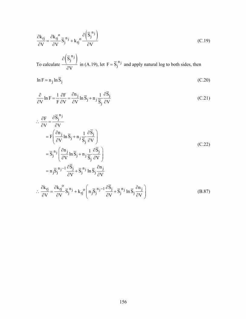
156
( )jj
no jnrj rj oj rj
Sk kS k
V V V
∂∂ ∂= +
∂ ∂ ∂ (C.19)
To calculate ( )jn
jS
V
∂
∂ in (A.19), let jn
jF S= and apply natural log to both sides, then
j jln F n ln S= (C.20)
j j
j jj
n S1 F 1ln F ln S nV F V V S V
∂ ∂∂ ∂= = +
∂ ∂ ∂ ∂ (C.21)
j
j
j j
nj
j jj j
j
n j jj j j
j
n 1 nj jj j j j
SFV V
n S1F ln S nV S V
n S1S ln S nV S V
S nn S S ln S
V V−
∂∂∴ =
∂ ∂ ∂ ∂
= + ∂ ∂ ∂ ∂
= + ∂ ∂ ∂ ∂
= +∂ ∂
(C.22)
j j jo
n n 1 nrj rj j joj rj j j j j
k k S nS k n S S ln S
V V V V− ∂ ∂ ∂ ∂
∴ = + + ∂ ∂ ∂ ∂ (B.87)
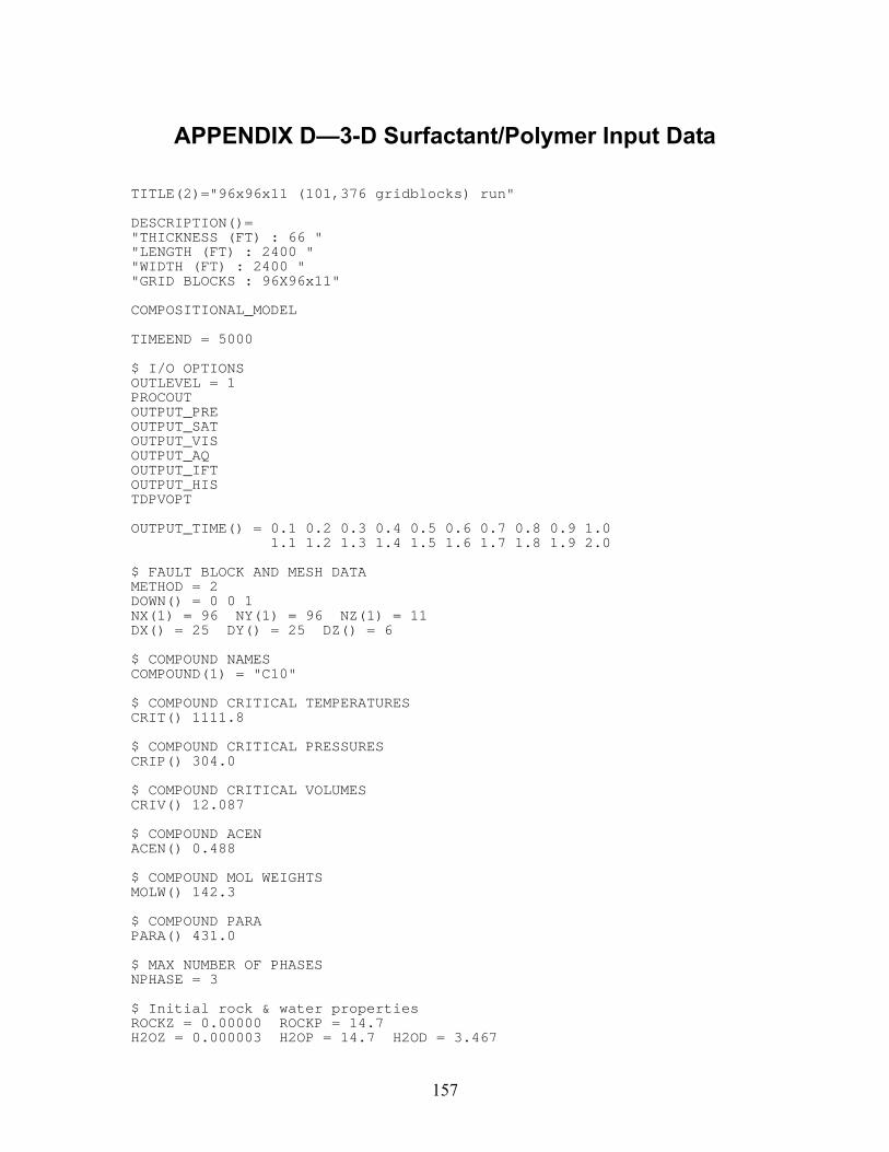
157
APPENDIX D—3-D Surfactant/Polymer Input Data TITLE(2)="96x96x11 (101,376 gridblocks) run" DESCRIPTION()= "THICKNESS (FT) : 66 " "LENGTH (FT) : 2400 " "WIDTH (FT) : 2400 " "GRID BLOCKS : 96X96x11" COMPOSITIONAL_MODEL TIMEEND = 5000 $ I/O OPTIONS OUTLEVEL = 1 PROCOUT OUTPUT_PRE OUTPUT_SAT OUTPUT_VIS OUTPUT_AQ OUTPUT_IFT OUTPUT_HIS TDPVOPT OUTPUT_TIME() = 0.1 0.2 0.3 0.4 0.5 0.6 0.7 0.8 0.9 1.0 1.1 1.2 1.3 1.4 1.5 1.6 1.7 1.8 1.9 2.0 $ FAULT BLOCK AND MESH DATA METHOD = 2 DOWN() = 0 0 1 NX(1) = 96 NY(1) = 96 NZ(1) = 11 DX() = 25 DY() = 25 DZ() = 6 $ COMPOUND NAMES COMPOUND(1) = "C10" $ COMPOUND CRITICAL TEMPERATURES CRIT() 1111.8 $ COMPOUND CRITICAL PRESSURES CRIP() 304.0 $ COMPOUND CRITICAL VOLUMES CRIV() 12.087 $ COMPOUND ACEN ACEN() 0.488 $ COMPOUND MOL WEIGHTS MOLW() 142.3 $ COMPOUND PARA PARA() 431.0 $ MAX NUMBER OF PHASES NPHASE = 3 $ Initial rock & water properties ROCKZ = 0.00000 ROCKP = 14.7 H2OZ = 0.000003 H2OP = 14.7 H2OD = 3.467
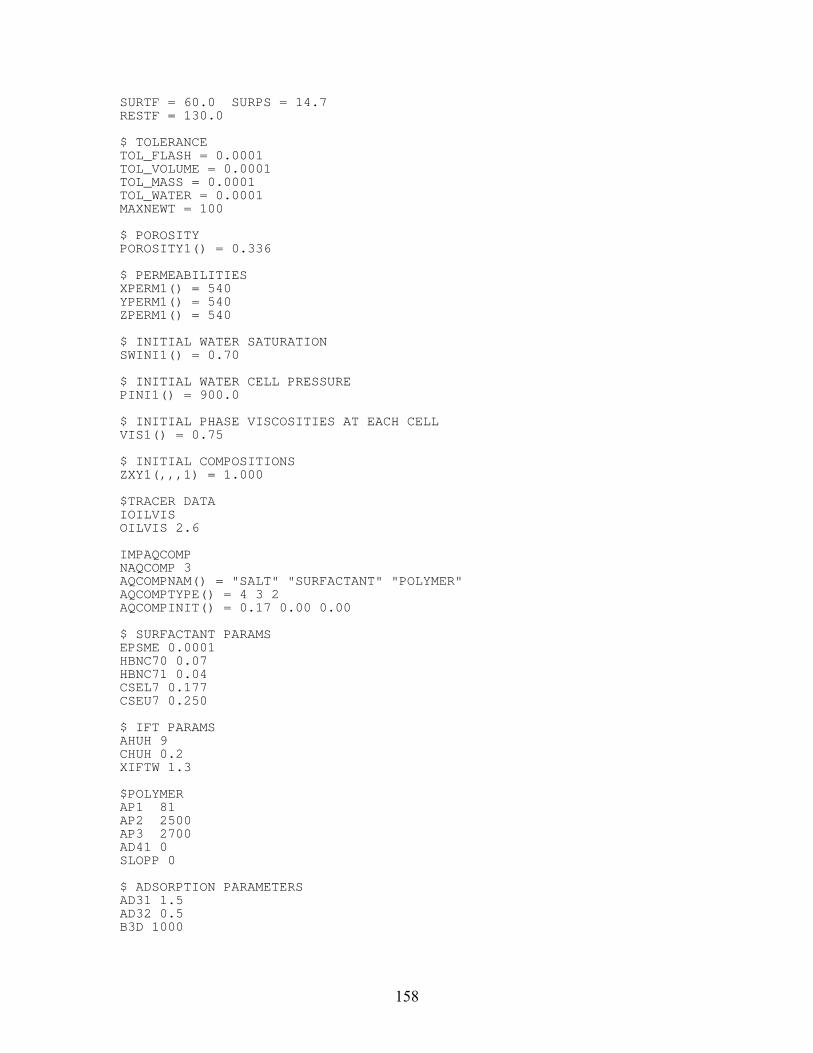
158
SURTF = 60.0 SURPS = 14.7 RESTF = 130.0 $ TOLERANCE TOL_FLASH = 0.0001 TOL_VOLUME = 0.0001 TOL_MASS = 0.0001 TOL_WATER = 0.0001 MAXNEWT = 100 $ POROSITY POROSITY1() = 0.336 $ PERMEABILITIES XPERM1() = 540 YPERM1() = 540 ZPERM1() = 540 $ INITIAL WATER SATURATION SWINI1() = 0.70 $ INITIAL WATER CELL PRESSURE PINI1() = 900.0 $ INITIAL PHASE VISCOSITIES AT EACH CELL VIS1() = 0.75 $ INITIAL COMPOSITIONS ZXY1(,,,1) = 1.000 $TRACER DATA IOILVIS OILVIS 2.6 IMPAQCOMP NAQCOMP 3 AQCOMPNAM() = "SALT" "SURFACTANT" "POLYMER" AQCOMPTYPE() = 4 3 2 AQCOMPINIT() = 0.17 0.00 0.00 $ SURFACTANT PARAMS EPSME 0.0001 HBNC70 0.07 HBNC71 0.04 CSEL7 0.177 CSEU7 0.250 $ IFT PARAMS AHUH 9 CHUH 0.2 XIFTW 1.3 $POLYMER AP1 81 AP2 2500 AP3 2700 AD41 0 SLOPP 0 $ ADSORPTION PARAMETERS AD31 1.5 AD32 0.5 B3D 1000
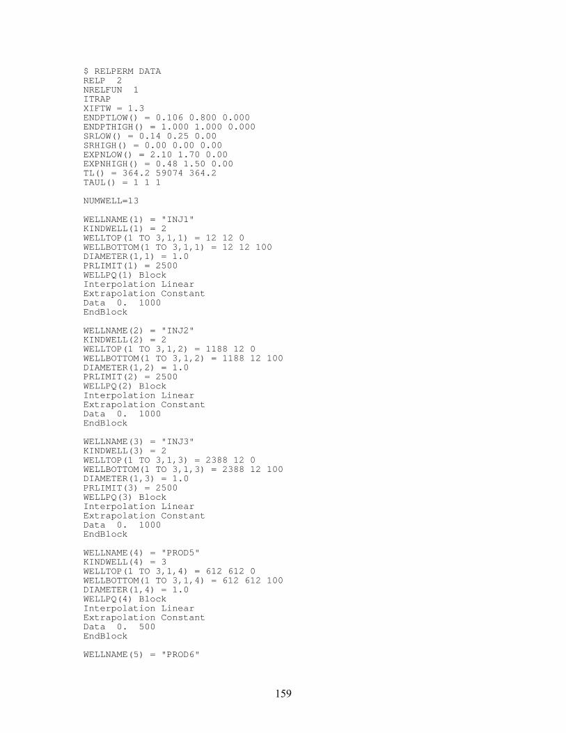
159
$ RELPERM DATA RELP 2 NRELFUN 1 ITRAP XIFTW = 1.3 ENDPTLOW() = 0.106 0.800 0.000 ENDPTHIGH() = 1.000 1.000 0.000 SRLOW() = 0.14 0.25 0.00 SRHIGH() = 0.00 0.00 0.00 EXPNLOW() = 2.10 1.70 0.00 EXPNHIGH() = 0.48 1.50 0.00 TL() = 364.2 59074 364.2 TAUL() = 1 1 1 NUMWELL=13 WELLNAME(1) = "INJ1" KINDWELL(1) = 2 WELLTOP(1 TO 3,1,1) = 12 12 0 WELLBOTTOM(1 TO 3,1,1) = 12 12 100 DIAMETER(1,1) = 1.0 PRLIMIT(1) = 2500 WELLPQ(1) Block Interpolation Linear Extrapolation Constant Data 0. 1000 EndBlock WELLNAME(2) = "INJ2" KINDWELL(2) = 2 WELLTOP(1 TO 3,1,2) = 1188 12 0 WELLBOTTOM(1 TO 3,1,2) = 1188 12 100 DIAMETER(1,2) = 1.0 PRLIMIT(2) = 2500 WELLPQ(2) Block Interpolation Linear Extrapolation Constant Data 0. 1000 EndBlock WELLNAME(3) = "INJ3" KINDWELL(3) = 2 WELLTOP(1 TO 3,1,3) = 2388 12 0 WELLBOTTOM(1 TO 3,1,3) = 2388 12 100 DIAMETER(1,3) = 1.0 PRLIMIT(3) = 2500 WELLPQ(3) Block Interpolation Linear Extrapolation Constant Data 0. 1000 EndBlock WELLNAME(4) = "PROD5" KINDWELL(4) = 3 WELLTOP(1 TO 3,1,4) = 612 612 0 WELLBOTTOM(1 TO 3,1,4) = 612 612 100 DIAMETER(1,4) = 1.0 WELLPQ(4) Block Interpolation Linear Extrapolation Constant Data 0. 500 EndBlock WELLNAME(5) = "PROD6"
160
KINDWELL(5) = 3 WELLTOP(1 TO 3,1,5) = 1812 612 0 WELLBOTTOM(1 TO 3,1,5) = 1812 612 100 DIAMETER(1,5) = 1.0 WELLPQ(5) Block Interpolation Linear Extrapolation Constant Data 0. 500 EndBlock WELLNAME(6) = "INJ8" KINDWELL(6) = 2 WELLTOP(1 TO 3,1,6) = 12 1188 0 WELLBOTTOM(1 TO 3,1,6) = 12 1188 100 DIAMETER(1,6) = 1.0 PRLIMIT(6) = 2500 WELLPQ(6) Block Interpolation Linear Extrapolation Constant Data 0. 1000 EndBlock WELLNAME(7) = "INJ9" KINDWELL(7) = 2 WELLTOP(1 TO 3,1,7) = 1188 1188 0 WELLBOTTOM(1 TO 3,1,7) = 1188 1188 100 DIAMETER(1,7) = 1.0 PRLIMIT(7) = 2500 WELLPQ(7) Block Interpolation Linear Extrapolation Constant Data 0. 1000 EndBlock WELLNAME(8) = "INJ10" KINDWELL(8) = 2 WELLTOP(1 TO 3,1,8) = 2388 1188 0 WELLBOTTOM(1 TO 3,1,8) = 2388 1188 100 DIAMETER(1,8) = 1.0 PRLIMIT(8) = 2500 WELLPQ(8) Block Interpolation Linear Extrapolation Constant Data 0. 1000 EndBlock WELLNAME(9) = "PROD12" KINDWELL(9) = 3 WELLTOP(1 TO 3,1,9) = 612 1812 0 WELLBOTTOM(1 TO 3,1,9) = 612 1812 100 DIAMETER(1,9) = 1.0 WELLPQ(9) Block Interpolation Linear Extrapolation Constant Data 0. 500 EndBlock WELLNAME(10) = "PROD13" KINDWELL(10) = 3 WELLTOP(1 TO 3,1,10) = 1812 1812 0 WELLBOTTOM(1 TO 3,1,10) = 1812 1812 100 DIAMETER(1,10) = 1.0 WELLPQ(10) Block Interpolation Linear
161
Extrapolation Constant Data 0. 500 EndBlock WELLNAME(11) = "INJ15" KINDWELL(11) = 2 WELLTOP(1 TO 3,1,11) = 12 2388 0 WELLBOTTOM(1 TO 3,1,11) = 12 2388 100 DIAMETER(1,11) = 1.0 PRLIMIT(11) = 2500 WELLPQ(11) Block Interpolation Linear Extrapolation Constant Data 0. 1000 EndBlock WELLNAME(12) = "INJ16" KINDWELL(12) = 2 WELLTOP(1 TO 3,1,12) = 1188 2388 0 WELLBOTTOM(1 TO 3,1,12) = 1188 2388 100 DIAMETER(1,12) = 1.0 PRLIMIT(12) = 2500 WELLPQ(12) Block Interpolation Linear Extrapolation Constant Data 0. 1000 EndBlock WELLNAME(13) = "INJ17" KINDWELL(13) = 2 WELLTOP(1 TO 3,1,13) = 2388 2388 0 WELLBOTTOM(1 TO 3,1,13) = 2388 2388 100