A new approach to understanding the

socio-economic determinants of fertility

over the life course

Maarten J. Bijlsma and Ben Wilson

Stockholm

Research Reports

in Demography

2017: 08

© Copyright is held by the author(s). SRRDs receive only limited review. Views and opinions expressed in SRRDs are

attributable to the authors and do not necessarily reflect those held at the Demography Unit.

2

A new approach to understanding the socio-economic

determinants of fertility over the life course

Maarten J. Bijlsma

Max Planck Institute for Demographic Research

Ben Wilson

SUDA, Stockholm University

Department of Methodology, London School of Economics

Abstract

Most theories of fertility predict that a range of socio-economic factors have an impact on the quantum and tempo of childbearing. Despite this, methods often struggle to investigate the interrelationships between these factors, and the time-varying influence that they have on fertility over the life course. In this study, we propose a new approach for studying the socio-economic determinants of fertility. This approach uses the parametric g-formula, which enables analyses of simultaneous and interdependent influences of time-varying socio-economic factors (such as education, employment and partnership) on fertility. Importantly, and unlike many other approaches, this method allows us to incorporate reverse causality and time-varying confounding in a study of total, direct, and indirect (mediating) effects. It also enables these effects to be generalized to a heterogeneous nationally-representative population, linking micro- and macro-level analyses, while avoiding the ecological fallacy. To demonstrate this approach, we study a cohort of women who were born in the UK in 1970. Our results show that a significant reduction in fertility rates would be produced by a reduction in marriage rates, and to a lesser extent by a rise in either education participation or full-time employment immediately after giving birth. For marriage, the majority of this effect is direct, rather than mediated by either education or employment. We conclude our analysis by demonstrating the sensitivity of results to unobserved confounding. We then discuss how our approach can be developed and applied in future research in order to provide researchers with a valuable tool for the analysis of total effects and mediation in studies of correlated life course processes.

3

Introduction

There are a range of interrelated socio-economic processes that influence childbearing over the life course (Balbo et al. 2012; Hirschman 1994). In order to understand and predict fertility, it is important to examine the links between these processes, and the collective impact that they have on childbearing (Buhr and Huinink 2014; Huinink and Kohli 2014). The socio-economic determinants of childbearing are a crucial component of most theories that have been used to explain fertility trends over the last fifty years. Even when they are not the theoretical focus, for example with respect to theories of norms and preferences, socio-economic determinants are usually essential mechanisms in both the expression and mediation of theoretical concepts (e.g. Andersson 2004; Forste and Tienda 1996; Johnson-Hanks et al. 2011; Lorimer 1956; Milewski 2010).

One of the most prominent demographic explanations for childbearing behaviour – the second demographic transition (SDT) – proposes that there are multiple explanations for fertility variation (Lesthaeghe 1983; van de Kaa 1987). These explanations include macro-level societal development, and micro-level changes in attitudes, values, and norms. But in order to understand the mechanisms through which fertility variation occurs, proponents of the SDT have also emphasised the importance of multiple socio-economic processes – such as partnership, education, and labour market participation – in collectively determining childbearing behaviour over the life course (Lesthaeghe 2010). These mechanisms are important, not least because they can help to explain the link between micro and macro, and therefore form a fundamental component of a complete and coherent explanation of population change (Billari 2015). For example, a better understanding of micro-level interrelationships between socio-economic factors may help to explain the reversal of fertility declines in high income countries (at the macro-level) (Myrskyla et al. 2009).

Demographers have shown a considerable interest in understanding how socio-economic processes collectively determine fertility (Balbo et al. 2012). Socio-economic decision-making lies at the heart of economic theories that consider the role of supply and demand for children (Becker 1981; Cleland and Wilson 1987; Easterlin and Crimmins 1985). Among other things, these theories predict that individuals – in particular women - will face a series of socio-economic trade-offs over their life course, including with respect to the timing of education, employment, partnership, and fertility (Billari and Kohler 2004; Dribe et al. 2014; Lee and Mason 2010). Along similar lines, recent sociological research has also emphasized the links between socio-economic choices and the timing of childbearing, in particular with respect to later-life opportunities. For example, research on ‘diverging destinies’ makes it clear that early life course decisions can have important consequences for later-life outcomes (Goisis and Sigle-Rushton 2014; Mclanahan 2004). For example, early childbearing is likely to have an indirect effect on future fertility via a number of socio-economic processes, like education (as well as possibly having a direct effect). Despite having a different theoretical framework, gender theories also emphasize the importance of interrelationships between different socio-economic processes – including fertility - in determining the trajectories of women’s lives (Neyer et al. 2013).

All of these theories predict that socio-economic processes determine fertility. Moreover, they also predict that socio-economic processes are interrelated, and that they determine fertility in a collective and simultaneous manner. However, what remains unclear, especially when examining the empirical literature, is how different socio-economic processes interact in order to collectively determine fertility over the

4

life course (for research that focuses on childbearing and one other correlated process, see: Kulu and Steele 2013; Kulu and Washbrook 2014; Steele et al. 2005). There is a growing body of research that shows how individual socio-economic processes, or aspects of these processes, have an influence on the tempo or quantum of fertility (Balbo et al. 2012). Nevertheless, little is known about the ways in which micro-level processes are linked together across women’s lives, and how these linkages determine individual childbearing trajectories (i.e. both tempo and quantum).

The importance of considering multiple determinants of fertility in a simultaneous analysis is also driven by methodological considerations. When investigating the role of individual theories in explaining fertility, or comparing the predictions of different theories, it is desirable to compare and contrast different explanations. Even when focussing on a single determinant, it is necessary to examine (or dismiss) competing explanations. For example, if we set out to study the effect of education on fertility, it is desirable to avoid inferring a false ‘education effect’, which might be the case if a correlation is spurious due to confounding. However, it can be difficult to account for confounding, whether by research design, statistical method, or by adjusting our interpretation (Doll 2002; Ní Bhrolcháin and Dyson 2007; Smith 2009). One common strategy is to design research that focuses on a single determinant and then exploit a source of ‘exogenous’ variation (external to the processes under investigation) that enables confounding to be discounted (given various assumptions) (Balbo et al. 2012; Engelhardt et al. 2009; Moffitt 2003, 2005). However, this strategy places a number of restrictions on the inferences that can be made, and does not allow the analysis of multiple determinants. Furthermore, it is even more problematic to examine multiple socio-economic determinants of fertility over the life course, where both the determinants and the outcome are time-varying.

Socio-economic determinants like partnership, education, and employment are complex, path-dependent and interrelated. As a consequence, they are hard to disentangle, and their influence on fertility is hard to study, even when drawing upon the range of methods that are available to social scientists (discussed further in the following section). Moreover, fertility is itself a complex and path-dependent process. It is distinct from most other social outcomes due to its (biological) restriction to a particular stage of the life course, and the fact that it represents a long-run weakly monotonic process of (exposure to) rare and highly interdependent (birth) events. By implication, past childbearing behaviour is likely to have an impact on future childbearing. At the same time, past childbearing is also likely to have an impact on future socio-economic outcomes. This is often referred to as reverse causality. Similarly, time-varying socio-economic processes can be mediators, which means that they can act as both causes and effects of fertility.

Given these issues, the application of causal inference methods to the study of fertility is not necessarily a straightforward task. It is neither plausible nor ethical to randomise the most prominent (or theoretically relevant) determinants of fertility, such as partnership formation or dissolution, employment or unemployment. Furthermore, observational studies typically sacrifice the ability to generalise (often called ‘external validity’), for a reduction in the number of threats to the validity of causal inferences (i.e. improved ‘internal validity’). It seems reasonable to suggest that demographers, perhaps more than other social scientists, are unhappy to make this trade-off, not least because of our interest in making statements about entire populations, which are a composite of the heterogeneous behaviour of all individuals.

5

In this study, we therefore propose a new approach to the study of fertility determinants. This approach enables us to estimate the influence of multiple interrelated factors – allowing for selection, reverse causality, and mediation – while simultaneously investigating the generalizable impact of plausible scenarios on a heterogeneous population. We make use of advanced methods for causal inference that have been developed by epidemiologists and biostatisticians in the last two decades. These methods, explained in more detail below, are particularly suited to research on the determinants of fertility because they were developed to enable researchers to test hypothetical changes in life course processes while accounting for interdependency and mediation, thereby disentangling direct and indirect effects.

The main aim of this research is therefore to demonstrate how these methods can be applied to studies of life course fertility. In order to provide an overview of the methods, and their potential benefits for studying fertility determinants, we carry out a case study of childbearing in the UK. Our guiding research question is: What are the effects of employment, education, and partnership on birth risks over the life course for a nationally-representative population? We also examine the intergenerational effects of parental fertility, and investigate the role of mediation and unobserved confounding in explaining our results. In the next section, we introduce our approach. We then describe how it relates to other methods that are commonly used to study fertility, before carrying out our case study of the UK. Finally, we conclude by discussing the strengths and weaknesses of our approach for future research on the socio-economic determinants of fertility.

Methodological background to our approach

The study of fertility can be seen, at least in part, as an ongoing effort to understand the factors that influence human reproduction (Becker et al. 1960; Cleland and Wilson 1987; Coale and Watkins 1986; Davis and Blake 1956; Kuczynski 1932). We refer to these factors as determinants. The importance of understanding these determinants might explain why fertility researchers have become increasingly concerned about causality, and why recent research has called for an increased focus on causal inference methods for the study of childbearing (Balbo et al. 2012). In essence, prior research has argued that causal explanations for fertility – at the level of individuals, groups or populations – can only be established with greater validity by taking methodological issues more seriously (Balbo et al. 2012; Billari 2015; Kulu and González-Ferrer 2014). Furthermore, there have been a number of significant and relatively recent methodological developments across the social sciences with respect to causal inference (Angrist and Pischke 2008; Engelhardt et al. 2009; Hernán and Robins 2006a; Imbens and Rubin 2015; Morgan and Winship 2007; Pearl 2009; Sampson et al. 2013; VanderWeele 2015; Vanderweele and Vansteelandt 2009).

One of the key developments in causal inference methodology is the potential outcomes framework (Holland 1986; Rubin 1974). In summary, this framework enables researchers to conceptualise counterfactuals, so that the effect of a cause can be compared with the effect in absence of this cause. This conceptualisation can be used in a variety of ways to identify and estimate potential (counterfactual) outcomes. In the example of a randomised experiment, with a single exposed group and a single control group, we observe the outcome Y for the exposed group (X=1), in counterfactual notation Y(x=1), but not their (hypothetical) potential outcome if not exposed, Y(x=0). However, we can estimate this potential outcome using observations from the control group, who are similar to the treated group (on average) due to randomisation.

6

The logic of potential outcomes is therefore analogous to a ‘what if’ scenario, and the same logic can be applied to mediation. This enables the comparison of observed patterns of mediation to their unobserved counterfactuals, in absence of mediation (Imai et al. 2010; Vansteelandt 2012). This may be fairly straightforward to conceptualise in the case of a time-constant binary exposure (as in a classical randomised experiment) and a single binary mediator at a single point in time, which implies four potential outcomes (i.e. Yx=1,m=1, Yx=1,m=0, Yx=0,m=1, Yx=0,m=1) (VanderWeele 2015). However, the number of potential outcomes becomes far greater when exposure and/or mediation is time-varying. In turn, this poses methodological challenges for research design and analysis (Robins 1986; Robins and Hernán 2009).

One way to help conceptualise complex (time-varying) causal processes is to make use of graphical models, in particular Directed Acyclic Graphs (DAGs) (Glymour 2006; Pearl 1995). The benefit of DAGs is that they enable the formal derivation of estimators (statistical models) of causal interrelationships based on subject-matter knowledge (Greenland et al. 1999). Essentially, the DAG makes explicit the processes and variables that are being investigated, and assumptions about the causal relationships between them. Importantly, there is also a direct correspondence between the theory of causal graphs and another series of methods, based on the work of Robins, which allow researchers to examine the role of time-varying confounding, mediation, and reverse causality (Greenland et al. 1999; Robins 1986; Robins and Hernán 2009). One of the most flexible of these methods is the parametric g-formula (Daniel et al. 2013; Keil et al. 2014; Robins and Hernán 2009). Our application of this method is described in detail below (see Methods), but in general it can be summarised as a series of three analytical steps:

1. Causal diagram: Draw a diagram (DAG) to describe the causal interrelationships that are being studied. This diagram describes the relationships that are assumed to exist between observed variables. By implication, it also shows which variables are unobserved, and which relationships are assumed not to exist (usually based on what is excluded from the diagram).

2. Estimation: Based on the DAG, a series of models are estimated using observed data (e.g. survey data). These models can take any parametric (functional) form, and the number of models will depend upon the number of variables (or more specifically the number of processes) that behave as outcomes.

3. Simulation: Estimated parameters from these models are then used to simulate a series of causal processes. Results may include, but are not limited to: (i) estimation of total effects under different scenarios, (ii) estimation of direct and indirect effects for these scenarios, and (iii) sensitivity analyses, for example to examine the role of unobserved confounding.

The parametric g-formula has several advantages over many of the methods that are currently used to study the determinants of fertility. It makes assumptions about observed and unobserved causal relationships explicit, uses real data, and applies parametric models with full flexibility (e.g. with respect to variable types, interactions, etc.). Another advantage is that it enables researchers to model time-varying processes while allowing for selection, reverse causality, and mediation. For example, the g-formula has allowed researchers to create an unbiased estimate of the effect of drug treatment on mortality, and disentangle direct and indirect effects, even in the presence of mediation due to relapse after treatment has begun (Keil et al. 2014).

7

Estimating the determinants of fertility

Over the last few decades, many new approaches have been applied in order to study the determinants of childbearing while accounting for confounding and reverse causality (Balbo et al. 2012). Typically, these approaches focus on isolating the effect of a single determinant on childbearing. For example, McCrary and Royer use school-entry policies to identify the impact of education on fertility (2011). Researchers have employed a range of methods that seek to isolate individual determinants, including difference-in-differences (DID), instrumental variables (IV), and regression discontinuity designs (RDD) (e.g. Aksoy and Billari 2015; Billari and Galasso 2009; Duclos et al. 2001; Lavy and Zablotsky 2011; McCrary and Royer 2011; Monstad et al. 2008). These methods have a number of advantages, if their assumptions are met. However, they also have a number of disadvantages, depending upon the nature of the research questions that are under investigation.

One disadvantage is that many of these methods sacrifice generalizability, and are restricted, in the absence of further assumptions, to making statements about narrow and sometimes unidentified groups (Hernán and Robins 2006b; Keil et al. 2014; Robins and Hernán 2009). For example, rather than estimating the average treatment effect for the population, some methods estimate a treatment effect for a subpopulation of the treated (with DID), or for compliers (with IV), or for a localized group of individuals who are close to a threshold (with RDD) (Angrist and Pischke 2008; Imbens and Rubin 2015). In contrast, the g-formula can estimate the population-level impact of changes to different determinants. It does this by modelling, and averaging over, micro-level processes.

With respect to fertility research, methods like IV, DID, or RDD may be more appropriate for studying certain research questions, for example to estimate the localised impact of a time-specific policy intervention that was not, or could not be randomised (Hernán et al. 2008; Khandker et al. 2009). However, these methods are far less suited to investigating the influence of multiple determinants over the life course. In fact, there are very few methods that are easily applied to studies of the inter-relationships between multiple time-varying determinants and a time-varying outcome, which is a situation that involves many sources of mediation (e.g. Clarke and Windmeijer 2012; Hernán and Robins 2006b).

One alternative to more static approaches is to use longitudinal approaches, such as ‘fixed-’ or ‘random-’ effects designs (Clarke et al. 2010; Gardiner et al. 2009). Fixed-effects approaches, including sibling or twin designs, are common in fertility research (Nisén et al. 2014; Tropf and Mandemakers 2017), but either suffer from the same generalizability issues already mentioned, or prevent the study of mediating interrelationships over the life course. A different approach for analyzing life course fertility is to use random-effect multi-process models. These models have been used to analyze the interrelationships between partnership and fertility (Steele et al. 2005), housing and fertility (Kulu and Steele 2013), and migration and fertility (Kulu and Washbrook 2014). This approach has a number of advantages over other approaches, not least because it enables the estimation of population-averaged effects. However, it relies on somewhat strict identification assumptions that make it difficult to model more than two processes simultaneously. Identification either requires that individuals experience repeated events in each of the simultaneous equations, or it requires the existence of an instrumental variable (Steele et al. 2005). In addition, and in common with other longitudinal approaches, including fixed- or random-effects, multi-process models do not model the reverse causal pathway (Steele et al. 2005).

8

In response to some of the above issues, researchers have also used a range of simulation-based methods to study the determinants of fertility. These methods tend to move away from design-based or model-based inference, to investigate causal explanations and causal mechanisms using micro-simulations or agent-based models (ABM) (Billari and Prskawetz 2003; Hernán 2015). Although there are some similarities between these existing approaches and the g-formula, in that they both make use of computer simulation. However, the principal difference is that the g-formula is grounded in the philosophy, and formal mathematical language, of causal inference. In turn, this brings a number of benefits, not least that it enables researchers to draw upon a vast and ever-growing literature on causal inference in order to carry out a more rigorous approach to the investigation of causality.

A case study of the UK

In order to demonstrate our approach, we carry out an analysis of life course childbearing in the UK. In common with most high-income countries, the UK has experienced a considerable shift in demographic behaviours over the last fifty years. Many of these changes align with, or might be explained by, the second demographic transition (SDT). The UK has experienced most of the interrelated changes that are predicted by the SDT, including a rise in cohabitation, divorce, and childbearing outside marriage (Beaujouan and Ní Bhrolcháin 2011; Berrington and Diamond 2000; Sigle-Rushton 2008; Wilson 2009; Wilson and Smallwood 2008). Relative to the rest of Europe, fertility in the UK has remained high, although there are considerable socio-economic differences in both the quantum and tempo of childbearing (Berrington 2004; O’Leary et al. 2010; B. Perelli-Harris et al. 2010; Brienna Perelli-Harris et al. 2012; Sigle-Rushton 2008). This includes a strong association between birth timing and socio-economic status (postponement of birth for high SES groups), as well as higher completed fertility among women who are in the lowest and highest socio-economic groups (as compared with those in between) (Sigle-Rushton 2008).

In this analysis, we focus on a specific cohort of women who were born in 1970. Since this cohort began their childbearing, there have been a number of changes in the observed associations between childbearing and the most commonly studied socio-economic factors (Berrington et al. 2015; Berrington and Pattaro 2014; Hobcraft 1996; Kneale and Joshi 2008; O’Leary et al. 2010; Rendall and Smallwood 2003; Steele et al. 2005, 2006). The most dramatic changes that are believed to determine these trends, and aggregate fertility patterns at the population level, include an increased participation in higher education among women, an increase in female employment, and a reduction in the prevalence of marriage (Chamberlain and Gill 2005; ONS 2016; Sigle-Rushton 2008).

Our data come from the 1970 British Cohort Study (BCS70), which follows the lives of around 17,000 people born in a single week of 1970 (UK Data Archive 2016). The sample covers Great Britain, which includes all of the constituent countries of the UK (England, Scotland and Wales), except for Northern Ireland. We study a subset of women in BCS70, and focus on their entire childbearing life course – all births - up to the age of 38 (the next wave data at age 42 were not yet readily available when we applied for access). According to recently released statistics based on all registered births in England and Wales, this cohort of women had an average completed fertility of 1.9 children per woman at age 45, (compared with 1.8 children ever born at age 38) (ONS 2016).

9

Alongside fertility, the main processes that we study are education, partnership, employment, and socio-economic status. Each process is measured using annual time-varying indicators based on derived variables from BCS70. In addition to time-varying measures, we include a number of time-constant ‘baseline’ characteristics. To examine the intergenerational transmission of fertility we include mother’s age at birth and number of siblings. The former is mother’s age when she gave birth to the woman who is being studied. The latter is calculated using information recorded at age 16 on number of siblings. We note that this may be slightly underestimated, due to unrecorded or unacknowledged siblings, or it may be overestimated due to the inclusion of step-siblings (although for 90% of respondents this variable is based on questions that ask about ‘blood brothers and sisters’). As a measure of parental resources, we use household income at age 10, and as a measure of spatial selection we use region of residence at age 16.

After dropping all women who are not in the dataset (or missing information on all variables) at the start of our observation period (age 16), we are left with approximately 4,100 women. After this, we drop all cases who have missing data on any one of our baseline covariates, which reduces the sample by around 21% to just over 3,200 women. There are no further changes to the analytical sample, such that we carry out complete case analysis, with the addition that women are censored from the year in which they cease to have complete information on all time-varying variables in the analysis.

Method

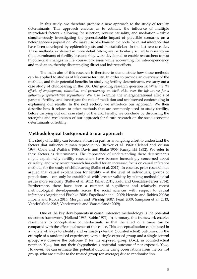
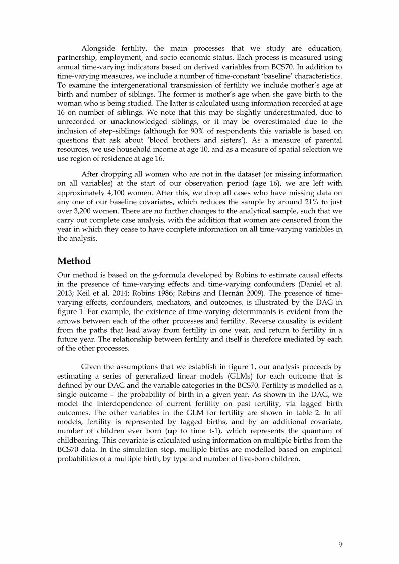
Our method is based on the g-formula developed by Robins to estimate causal effects in the presence of time-varying effects and time-varying confounders (Daniel et al. 2013; Keil et al. 2014; Robins 1986; Robins and Hernán 2009). The presence of time-varying effects, confounders, mediators, and outcomes, is illustrated by the DAG in figure 1. For example, the existence of time-varying determinants is evident from the arrows between each of the other processes and fertility. Reverse causality is evident from the paths that lead away from fertility in one year, and return to fertility in a future year. The relationship between fertility and itself is therefore mediated by each of the other processes.

Given the assumptions that we establish in figure 1, our analysis proceeds by estimating a series of generalized linear models (GLMs) for each outcome that is defined by our DAG and the variable categories in the BCS70. Fertility is modelled as a single outcome – the probability of birth in a given year. As shown in the DAG, we model the interdependence of current fertility on past fertility, via lagged birth outcomes. The other variables in the GLM for fertility are shown in table 2. In all models, fertility is represented by lagged births, and by an additional covariate, number of children ever born (up to time t-1), which represents the quantum of childbearing. This covariate is calculated using information on multiple births from the BCS70 data. In the simulation step, multiple births are modelled based on empirical probabilities of a multiple birth, by type and number of live-born children.

10

Figure 1: Directed acyclic graph of fertility and time-varying mediating confounders

Each arrow represents a causal relationship in the direction indicated by the arrow. Only the relationships between age 16 and 18 are shown since the relationships are the same from each year to the next. Note that time-constant baseline characteristics – parental income, mother’s age at birth, number of siblings, and region – are not shown because these are modelled to have a direct effect on every time-varying process in every year. The same is true of age. All models include interactions between age and partnership, fertility and education, fertility and partnership, and fertility and employment. Fertility is modelled using ‘birth in a given year’, and the lagged equivalent as shown. This outcome is then adjusted to account for multiple births, which enables a cumulative count of ‘children ever born’ to be estimated and used as a control variable in each of our simultaneous equations.

In parallel with the GLM for fertility, we estimate similar models for the following outcomes: cohabitation, marriage, not having a partner, not being employed, part-time employment, full-time employment, full-time education, being permanently disabled. Essentially, we model the conditional probability of each component of the contemporaneous time-varying processes illustrated in figure 1. The covariates in each of these models are shown in table 2. We use a logistic specification for all GLMs. In the simulation step of the g-formula these models are used to produce probabilities for each outcome, and multinomial variables are then predicted as a single outcome. The estimation of these models is part of the g-formula, which can be summarized as follows:

Estimation steps of the g-formula

step 1: draw one random sample of individuals with replacement from the data

step 2: estimate models

step 3: draw a dataset for starting values at baseline / ‘first’ year

step 4: calculate outcomes for the ‘second’ year

step 5: repeat step 4 for all years, given values at the previous year

step 6: save results and go back to step 1

step 7: repeat steps 1-6 for each iteration (999 times)

step 8: report the estimates and corresponding uncertainty

11

Once this process is complete, we obtain estimates of what is usually referred to as the ‘natural course’. The natural course is not exactly the same as the empirical data, but should approximate it, and is essentially a simulation of the empirical data with uncertainty (see step 1 above). It can be conceptualized as the natural (observed) state of the BCS70 population, in absence of any intervention or counterfactual scenario. To put it another way, the natural course is essentially an estimate of causal interrelationships – their magnitude and uncertainty – based on the empirical data. Given the representativeness of the sample, they can then be used for population inference in the tradition of classical statistics. However, this task is made more difficult than in many multivariate settings because of the complex interdependencies, such that it is unclear how one parameter can be interpreted in isolation (somewhat similar to trying to interpret only the main effect of a full interaction).

Given this difficulty of interpreting individual parameters, the g-formula is almost always used to estimate changes in the outcome of interest – e.g. fertility – under one or more hypothetical, plausible, and scientifically-relevant scenarios. This is appealing on a number of grounds, not least because it aligns with the philosophy of counterfactuals and potential outcomes (since each scenario effectively asks what the potential outcome would be under alternative conditions). In fact, the g-formula was specifically designed to enable researchers to estimate the causal impact of different scenarios or interventions.

Table 1: Estimated scenarios

Scenario Details

1: Increase in higher education attendance

We randomly select a group of women from those who are still in education at age 16, and then keep them in education until age 22, so that at least 50% of all women remain in (higher) education until age 22.

2: Reduction in the preference for marriage

We simulate a decrease in the proportion of women who are married, and a corresponding increase in the proportions single and cohabiting, equivalent to a 50% reduction in the stock of married women over the study period.

3: Increase in post-birth employment

We adjust the employment probabilities to ensure that all women, except those who are disabled, are employed full-time in the year after their birth (after which time they are free to follow any employment trajectory).

4: The impact of having no siblings / being an only-child

We create a scenario where all women have no siblings and examine the impact of this on their fertility. This examines the intergenerational impact of low fertility, assuming that all women were an only-child.

In our case, we examine the impact of four scenarios on fertility, each of which is shown in table 1, alongside the details of how this scenario is implemented. The motivation behind each of these scenarios is slightly different. The first two set out to examine the effect of large-scale demographic changes on fertility. These scenarios are based on observed trends in the UK from 1970 until the present day: increases in higher education attendance among women (scenario #1), and a reduction in the preference for marriage (#2). In addition to these trend-based scenarios, we examine the effect of a hypothetical invention to increase the post-birth employment of women (#3). This is chosen in order to demonstrate how this method might be used to examine the potential impact of a specific policy.

12

Finally, we also examine the effect of a change in background conditions, as mediated by time-varying factors. Here, we focus on the effect of parental fertility (#4). In this case, our principal motivation is to examine whether there is an impact of low fertility on the fertility of future generations.

The results of each of these scenarios is calculated by re-estimating the g-formula (see the aforementioned steps), while making the respective changes that refer to the specifics of each scenario. These are then compared against the natural course (with uncertainty) in order to derived estimates of the impact of each scenario. Given that confidence intervals can be calculated for each observed period (i.e. annually), the statistical significance of each scenario can be calculated at each age over the life course.

The rest of our analysis then focuses on two issues: mediation and unobserved confounding. Our mediation analysis focuses on two scenarios (#2 and #4). For both scenarios, we estimate the direct and indirect effect of each intervention on fertility. This is essentially a decomposition of the total effect, (which in counterfactual notation is E[Yx=1–Yx=0], where X=1 is the scenario and X=0 is the natural course). However, it is important to note that there are different definitions of direct and indirect effects in the literature, and different ways of estimating their values (Lin et al. 2017; Suzuki et al. 2014; VanderWeele 2015; Vanderweele and Vansteelandt 2009; Wang and Arah 2015).

In our analysis, we decompose the total effect into the controlled direct effect (CDE) and the proportion eliminated (PE). The CDE is determined like the TE, except the values of mediating variables are drawn at random from the natural course (i.e. E[Yx=1,m*–Yx=0,m*]), so that the effect of the scenario of interest on the outcome can no longer go through these mediators and is thus only a ‘direct’ effect. For example, changes in the preference for marriage can now only affect fertility directly, and not via employment because values for employment are drawn randomly from the natural course. The PE is calculated as TE – CDE and represents the part of the scenario effect that goes through the mediators. It is important to note that the CDE and PE can only be calculated based on mediators that are free to vary in any given scenario. For example, partnership cannot be a mediator in the marriage scenario.

In the final part of our analysis, we examine the sensitivity of our results to unmeasured confounding (Robins et al. 2000). To do this, we focus on the scenario of a reduction in the preference for marriage (#2). We recognize that sensitivity analysis for causal inference is a relatively new topic, and there is no standard approach. Nevertheless, we draw upon recently proposed approaches to simulate the influence that a hypothetical unobserved confounder would have on our results (Carnegie et al. 2016; Lin et al. 2017; VanderWeele 2015). Our approach is described in more detail below (and in an appendix, which is available on request).

13

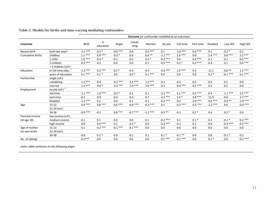
Table 2: Models for births and time-varying mediating confounders

Outcome (or confounder modelled as an outcome)

Covariate Birth In

education Single

Cohab-iting

Married No job Full-time Part-time Disabled Low SES High SES

Recent birth birth last year? -1.1 *** -0.5 * -0.6 *** 0.0 0.5 *** 0.1 -1.0 *** 0.6 *** -0.1 -0.2 * 0.1

Cumulative births childless 1.1 *** 0.9 *** -0.3 * 0.0 0.6 ** -2.1 *** 2.6 *** 0.0 2.4 *** 0.8 *** 2.2 ***

1 child 1.6 *** -0.5 * -0.1 -0.1 0.2 * -0.3 *** 0.0 0.4 *** 0.1 -0.1 0.5 ***

2 children 0.3 *** -0.2 0.0 0.0 0.1 -0.5 *** 0.2 * 0.4 *** -0.4 0.1 0.6 ***

> 3 children (ref.)

Education in full-time educ. 1 -1.3 *** 5.3 *** 0.5 * -0.3 -0.3 -4.5 *** 1.9 *** 0.3 -11.1 0.6 ** 1.1 ***

years of education 0.1 *** 0.1 * 0.0 0.0 * 0.1 *** 0.0 0.0 0.0 -0.2 * -0.1 *** 0.1 ***

Partnership single (ref.)

cohabiting 1.1 *** -0.4 -4.2 *** 3.4 *** 1.3 *** -0.1 -0.2 0.2 0.4 0.1 0.0

married 1.5 *** -0.6 * -5.4 *** -2.9 *** 7.0 *** -0.1 -0.6 *** 0.5 *** 0.2 0.2 0.0

Employment no job (ref.) 1

full-time -1.1 *** -1.0 *** -0.2 * 0.1 0.1 -5.3 *** 6.1 *** -0.5 *** 0.4 -1.1 *** 5.5 ***

part-time 0.2 -9.9 -0.5 -0.3 0.7 -4.5 *** 1.4 * 3.8 *** -11.9 0.8 2.7 ***

disabled -1.2 *** 0.1 0.0 0.1 -0.1 -6.5 *** -0.2 -2.0 *** 9.6 *** -0.9 ** -1.9 ***

Age 15-22 0.4 *** 0.8 *** 0.6 *** -0.6 *** -0.3 *** 0.1 -0.3 *** -0.3 *** -1.2 *** 0.0 -0.4 ***

22-29 (ref.)

30-38 -0.9 *** -0.1 0.8 *** -0.7 *** -1.2 *** -0.3 ** -0.1 0.2 * 0.4 0.2 * 0.0

Parental income low income (ref.)

(at age 10) medium income -0.1 0.1 0.0 0.0 0.1 -0.2 *** 0.1 0.1 * -0.1 -0.1 * 0.2 ***

high income -0.0 0.4 *** 0.1 -0.1 * 0.0 -0.2 *** -0.1 0.1 -0.4 -0.3 *** 0.2 ***

Age of mother 15-22 0.1 -0.2 *** -0.1 *** 0.1 *** 0.0 0.0 0.0 0.0 0.0 0.0 0.0

(at own birth) 22-29 (ref.)

30-38 -0.0 0.1 * 0.0 -0.1 0.1 0.1 * -0.1 ** 0.0 0.0 -0.1 * -0.1

No. of siblings 0.1*** 0.0 0.0 0.0 0.0 0.1 *** -0.1 *** 0.0 0.1 * 0.0 -0.1 ***

[note: table continues on the following page]

14

Outcome (or confounder modelled as an outcome)

Covariate Birth In

education Single

Cohab-iting

Married No job Full-time Part-time Disabled Low SES High SES

[note: table continued from previous page]

Region Scotland -0.2 * -0.1 -0.1 0.0 0.2 * -0.4 *** 0.3 *** -0.1 1.6 ** 0.2 0.2 *

Wales 0.2 -0.1 -0.2 ** 0.0 0.3 ** -0.1 0.1 0.0 2.0 *** 0.1 0.0

England: North -0.1 * -0.1 -0.2 ** 0.1 0.1 -0.3 *** 0.2 ** 0.0 1.1 * 0.1 0.1

England: Midlands -0.1 -0.1 -0.2 ** 0.1 0.2 * -0.2 * 0.1 0.0 1.3 ** 0.1 0.0

England: South -0.1 -0.1 -0.3 *** 0.1 * 0.1 -0.3 *** 0.1 * 0.1 1.0 * 0.1 0.2 *

England: London (ref.)

Interactions:

full-time employment: high SES 0.3 *** 0.1 0.0 0.1 * -0.2 ** 0.6 *** -0.6 *** 0.5 *** 1.2 *** 6.0 *** -5.4 ***

full-time employment: low SES -0.8 * 9.0 0.1 0.3 -0.3 -0.5 -0.9 0.8 * 12.1 -1.4 ** 2.4 ***

part-time employment: high SES -1.1 ** 9.4 0.1 0.6 -0.6 -0.3 -0.9 0.8 * 12.9 4.2 *** -2.9 ***

part-time employment: low SES -0.1 -0.6 ** -0.8 *** 0.8 *** 0.3 * 0.5 *** 0.0 -0.1 0.8 -0.2 0.0

15-22: cohabiting -0.3 * -0.6 -0.3 0.8 ** 0.1 0.4 ** 0.0 -0.3 0.8 -0.1 -0.2

15-22: married 0.7 *** -0.3 -1.4 *** 1.2 *** 0.8 *** 0.1 0.0 0.0 -1.2 ** -0.1 0.2

30-38: cohabiting 0.4 * -0.1 -1.0 *** -0.1 1.5 *** 0.0 0.3 ** -0.2 -0.4 -0.3 * 0.3 ***

30-38: married -0.9 ** -2.1 *** 0.3 -0.3 -0.8 * 0.7 ** -1.9 *** -0.4 10.7 -0.7 ** -1 ***

childless: in education -0.1 *** 0.0 0.0 0.0 * 0.0 * 0.0 ** 0.0 ** 0.0 * 0.1 0.0 0.0

childless: yrs of edu 0.4 *** 0.4 0.0 -0.4 *** 0.2 0.4 *** -0.2 0.2 -0.6 -0.2 * -0.1

childless: cohab 1.3 *** 0.3 0.1 0.4 * -0.5 ** 1.2 *** -0.7 *** 0.6 *** -0.4 -0.6 *** -0.6 ***

childless: married -0.5 *** -0.6 * 0.0 0.0 0.1 1.1 *** -2.1 *** -0.7 *** -2.2 *** -0.6 *** -1.3 ***

childless: full-time -0.4 ** 0.2 0.2 0.0 -0.1 1.1 *** -1.2 *** -0.4 ** -1.1 -0.9 *** -1.2 ***

childless: part-time -0.5 -1.7 * 1.1 *** -0.9 ** -0.4 1.3 * -2.5 *** 0.9 -2.2 *** -1.1 * -0.4

childless: disabled 0.3 *** 0.1 0.0 0.1 * -0.2 ** 0.6 *** -0.6 *** 0.5 *** 1.2 *** 6.0 *** -5.4 ***

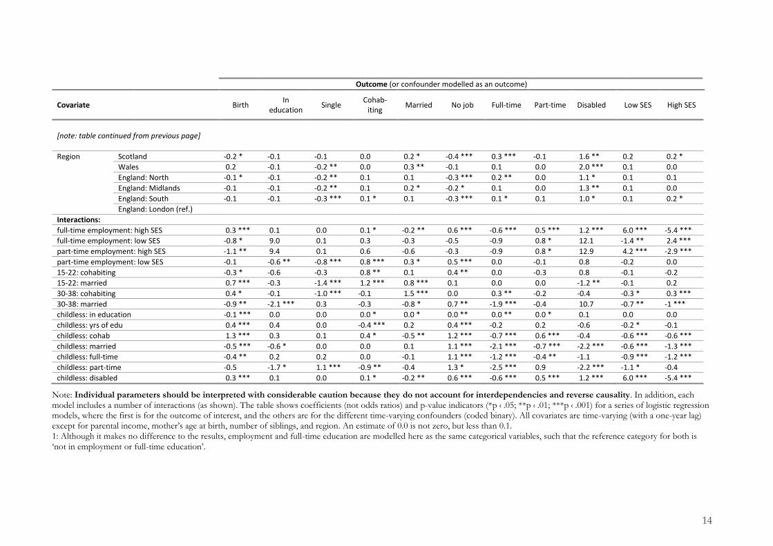
Note: Individual parameters should be interpreted with considerable caution because they do not account for interdependencies and reverse causality. In addition, each model includes a number of interactions (as shown). The table shows coefficients (not odds ratios) and p-value indicators (*p ‹ .05; **p ‹ .01; ***p ‹ .001) for a series of logistic regression models, where the first is for the outcome of interest, and the others are for the different time-varying confounders (coded binary). All covariates are time-varying (with a one-year lag) except for parental income, mother’s age at birth, number of siblings, and region. An estimate of 0.0 is not zero, but less than 0.1. 1: Although it makes no difference to the results, employment and full-time education are modelled here as the same categorical variables, such that the reference category for both is ‘not in employment or full-time education’.

15

Results from the conditional models

The results in table 2 show coefficients from a series of logistic regression models that estimate the causal relationships outlined in figure 1. For example, the first column of results is for a model of births (in a given year) conditional on the covariates that are specified in the first two columns. The results in table 2 cannot be interpreted causally, because they represent only one step of the g-formula procedure. This means that, although these models take account of time-varying confounding, the confounders are also mediators, so the interpretation of coefficients (conditional on covariates) is at best an indicative summary of a time-varying relationship.

Despite this cautionary note, some analysts refer to coefficients that are modelled by the g-formula as a means of checking that model specifications are coherently aligned with expectations. Unexpected values of parameters are not necessarily incorrect, but may warrant further investigation. In table 2, the coefficients demonstrate patterns of association in the BCS70 data, and they appear to align with the results of previous research (discussed above). For example, a decreased risk of birth is associated with being single, employed, or in full-time education.

In table 3, we show another form of model diagnostic, which is a comparison between the natural course and the empirical data with respect to (predicted) number of births. As with any other causal inference model, the aim of our approach is not to (perfectly) predict either the empirical data, or any future scenario, but rather to make causal inferences. Nevertheless, these are not unrelated tasks (including for many other causal inference approaches). An important diagnostic is therefore to examine the difference between the empirical data (BCS70) and the average predicted number of children from the g-formula (i.e. the natural course). This is shown in table 3, which highlights the main differences in our example. It appears that the g-formula does a good job of predicting cumulative fertility at age 38, although with some small differences from the empirical data. There is a slight underestimation of childlessness, although this may be due, in part, to the censoring in our empirical subsample.

Table 3: Comparison between natural course and empirical data

Proportion of women, by parity at age 38

0 1 2 3 4 5 6+

Natural course 22 20 39 15 3 1 0

Empirical data 24 20 37 14 4 1 0

Note: Empirical data is based on our analytical subsample, and therefore includes some censoring. In any case, these proportions are not expected to be the same (see text).

16

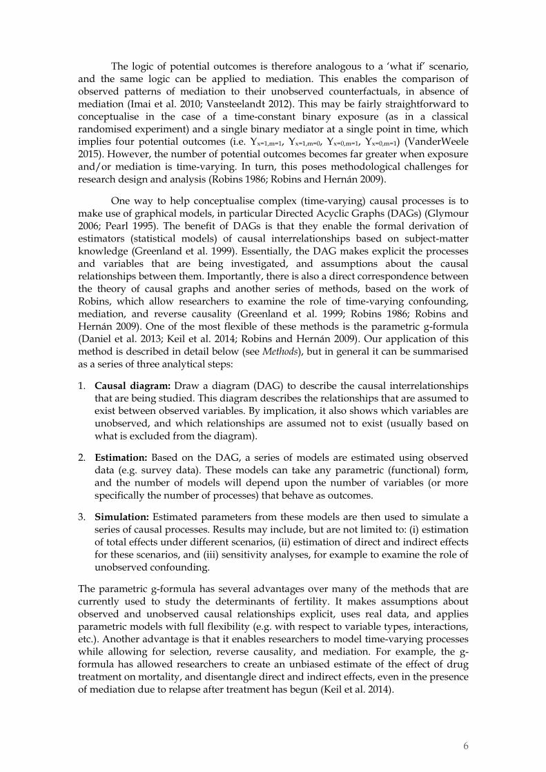
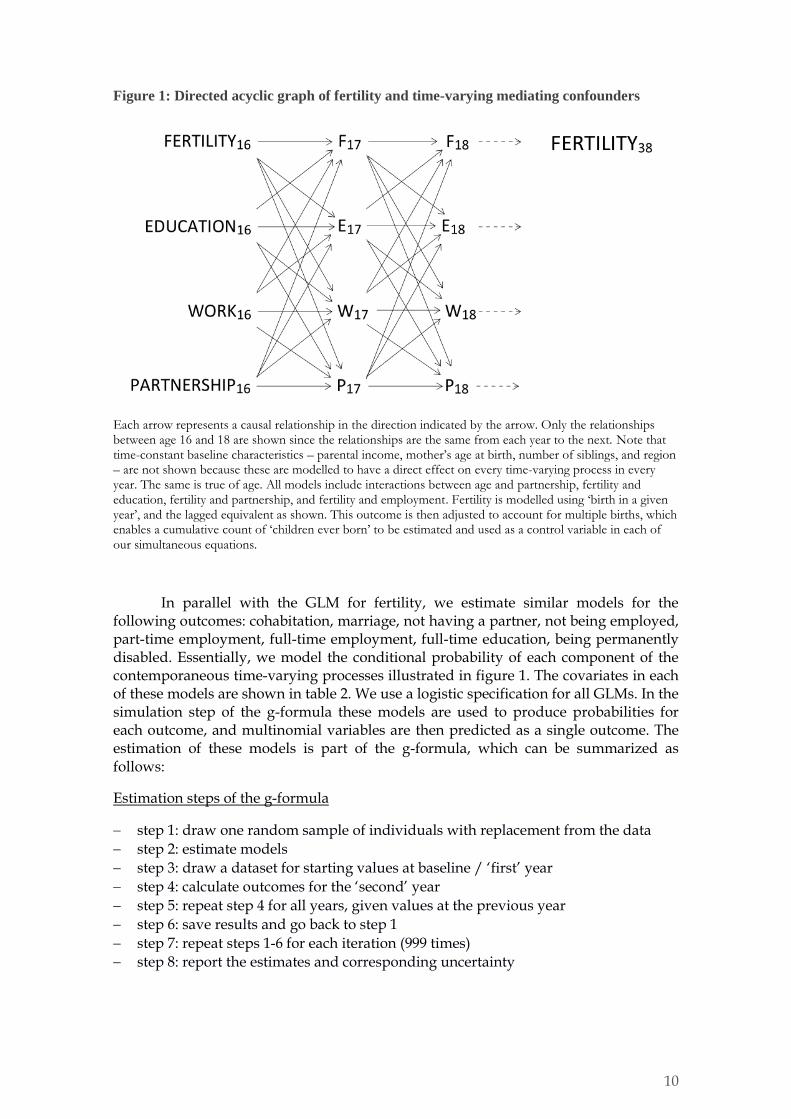
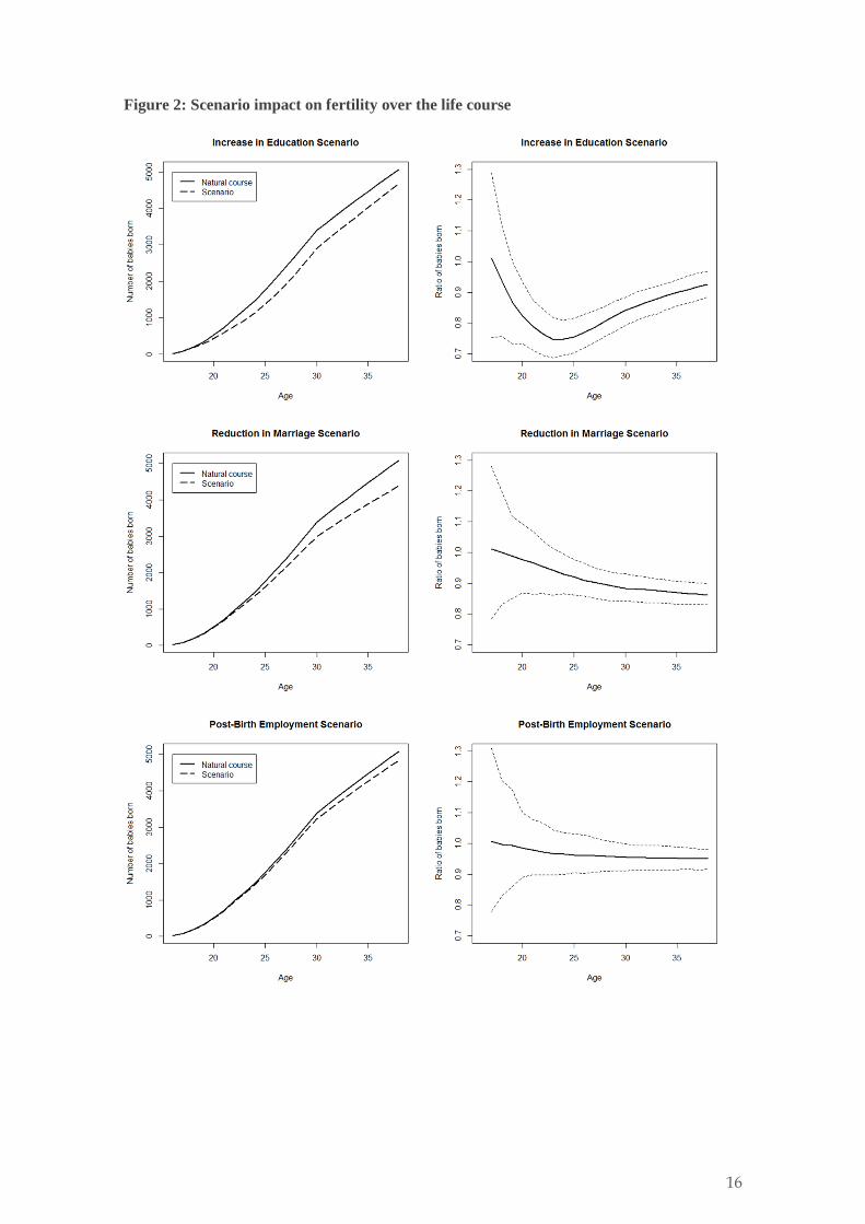
Figure 2: Scenario impact on fertility over the life course

17

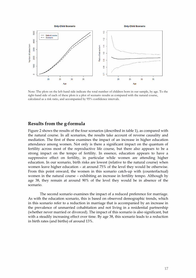
Note: The plots on the left-hand side indicate the total number of children born in our sample, by age. To the right-hand side of each of these plots is a plot of scenario results as compared with the natural course, calculated as a risk ratio, and accompanied by 95% confidence intervals.

Results from the g-formula

Figure 2 shows the results of the four scenarios (described in table 1), as compared with the natural course. In all scenarios, the results take account of reverse causality and mediation. The first of these examines the impact of an increase in higher education attendance among women. Not only is there a significant impact on the quantum of fertility across most of the reproductive life course, but there also appears to be a strong impact on the tempo of fertility. In essence, education appears to have a suppressive effect on fertility, in particular while women are attending higher education. In our scenario, birth risks are lowest (relative to the natural course) when women leave higher education – at around 75% of the level they would be otherwise. From this point onward, the women in this scenario catch-up with (counterfactual) women in the natural course – exhibiting an increase in fertility tempo. Although by age 38, they remain at around 90% of the level they would be in absence of the scenario.

The second scenario examines the impact of a reduced preference for marriage. As with the education scenario, this is based on observed demographic trends, which in this scenario refer to a reduction in marriage that is accompanied by an increase in the prevalence of unmarried cohabitation and not living in a residential partnership (whether never married or divorced). The impact of this scenario is also significant, but with a steadily increasing effect over time. By age 38, this scenario leads to a reduction in birth rates (and births) of around 13%.

18

In the third scenario, we examine the impact of a hypothetical invention to increase post-birth employment. The results of this scenario are similar to that of the marriage scenario, except that they are weaker. This might be expected because we only adjust employment rates in the year immediately after birth, and allow them to vary after that. However, it is also due to the relative strength of the (conditional) relationship between partnership and fertility as compared with employment and fertility. These scenarios could of course be specified in a number of different ways, but as specified, marriage appears to have a stronger underlying effect on fertility than full-time employment immediately after birth. Based on our assumptions, a policy that enabled full-time employment for all women in the first year after birth would result in around 5% fewer births.

In the last scenario, we examine whether low (parental) fertility has an impact on the fertility of the next generation. Our results show that if all women were an only child, with no siblings, then this would lead to a reduction in fertility. The size of this effect is fairly similar to the post-birth employment scenario, and it is likewise broadly monotonic (steadily decreasing) over the life course. It may be interesting to note that these results are in contrast to the results of another scenario (not shown here) in which we manipulated time-constant factors. Results were not significant in a scenario of upward mobility in parental income, (where we effectively took 50% of parents and placed them in a higher income category than the one they were in).

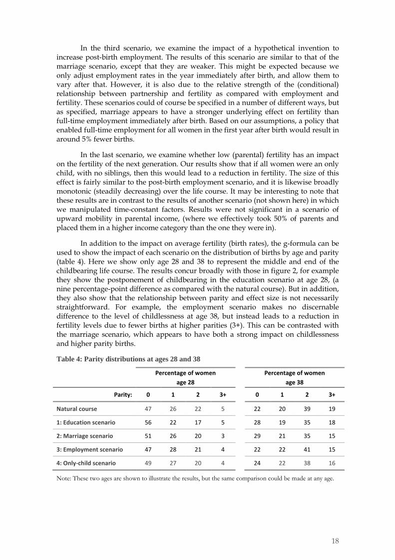
In addition to the impact on average fertility (birth rates), the g-formula can be used to show the impact of each scenario on the distribution of births by age and parity (table 4). Here we show only age 28 and 38 to represent the middle and end of the childbearing life course. The results concur broadly with those in figure 2, for example they show the postponement of childbearing in the education scenario at age 28, (a nine percentage-point difference as compared with the natural course). But in addition, they also show that the relationship between parity and effect size is not necessarily straightforward. For example, the employment scenario makes no discernable difference to the level of childlessness at age 38, but instead leads to a reduction in fertility levels due to fewer births at higher parities (3+). This can be contrasted with the marriage scenario, which appears to have both a strong impact on childlessness and higher parity births.

Table 4: Parity distributions at ages 28 and 38

Percentage of women Percentage of women

age 28 age 38

Parity: 0 1 2 3+ 0 1 2 3+

Natural course 47 26 22 5 22 20 39 19

1: Education scenario 56 22 17 5 28 19 35 18

2: Marriage scenario 51 26 20 3 29 21 35 15

3: Employment scenario 47 28 21 4 22 22 41 15

4: Only-child scenario 49 27 20 4 24 22 38 16

Note: These two ages are shown to illustrate the results, but the same comparison could be made at any age.

19

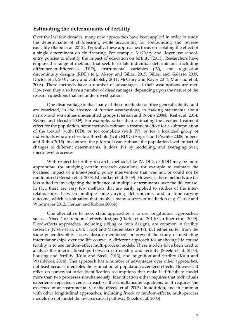
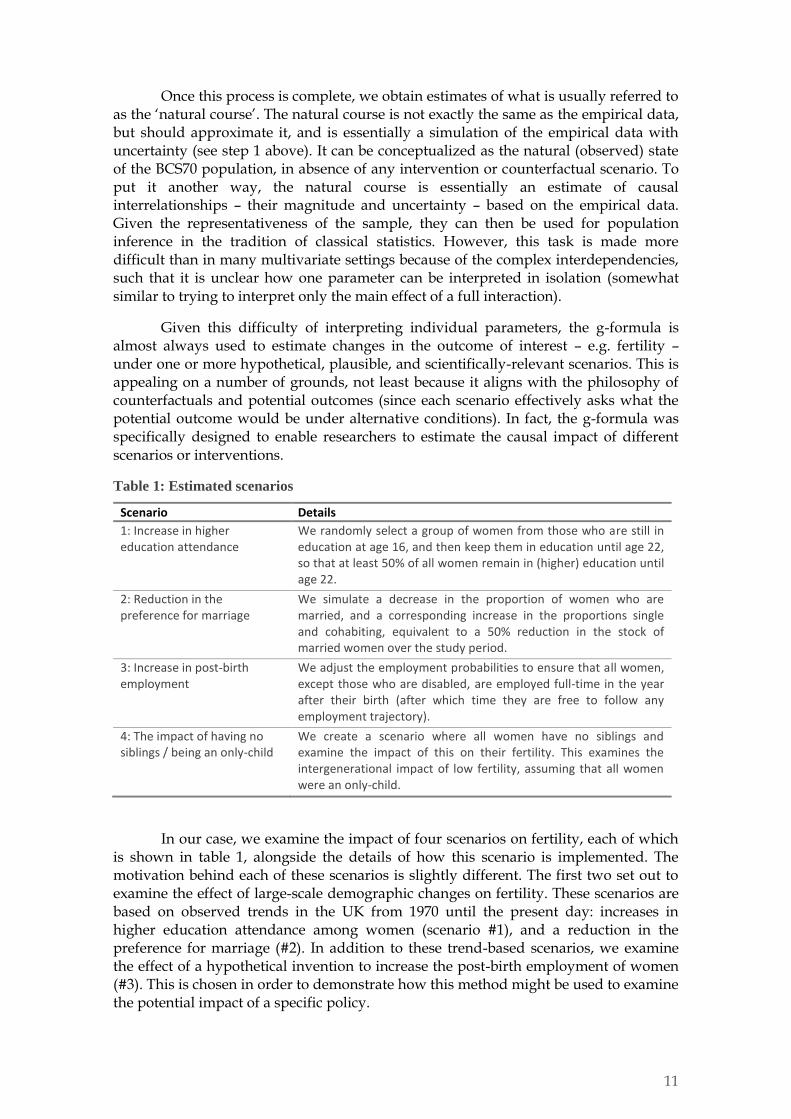
Figure 3: Controlled direct effect (CDE) and proportion eliminated (PE) as percentage of total effect (TE)

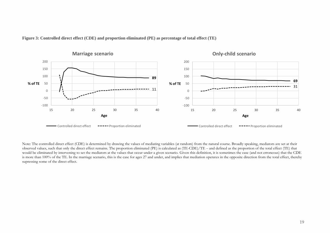
Note: The controlled direct effect (CDE) is determined by drawing the values of mediating variables (at random) from the natural course. Broadly speaking, mediators are set at their observed values, such that only the direct effect remains. The proportion eliminated (PE) is calculated as (TE-CDE)/TE – and defined as the proportion of the total effect (TE) that would be eliminated by intervening to set the mediators at the values that occur under a given scenario. Given this definition, it is sometimes the case (and not erroneous) that the CDE is more than 100% of the TE. In the marriage scenario, this is the case for ages 27 and under, and implies that mediation operates in the opposite direction from the total effect, thereby supressing some of the direct effect.

89

11

-100

-50

0

50

100

150

200

15 20 25 30 35 40

% of TE

Age

Marriage scenario

Controlled direct effect Proportion eliminated

69

31

-100

-50

0

50

100

150

200

15 20 25 30 35 40

% of TE

Age

Only-child scenario

Controlled direct effect Proportion eliminated

Mediation analysis

We performed two mediation analyses: one for the marriage scenario (#2) and one for the only-child scenario (#4). In both cases, the direct effect (CDE) is much larger than the indirect effect (PE) at all ages (figure 3). As a share of the total effect, the CDE does become smaller over time, and the PE larger, although the CDE remains relatively larger in both scenarios, even at age 38. It may be important to note that it is quite plausible (and not erroneous) that the CDE is more than 100% of the TE. In the marriage scenario, this is the case for ages 27 and under, and implies that mediation operates in the opposite direction from the total effect, thereby suppressing some of the direct effect.

Comparing the two scenarios, the direct effect is relatively smaller in the only-child scenario (around 70% of the total effect at age 38), as compared with the marriage scenario (90% of TE at age 38). This is perhaps unsurprising given that the marriage scenario is a time-varying intervention, such that we might expect a large direct effect because the scenario is essentially comprised of a series of direct effects that repeat over the life course. Among other things, this highlights the likely importance of differentiating between time-constant and time-varying scenarios. Or, from a policy-perspective, it implies that time-constant interventions may be more likely to be mediated than time-varying interventions. The approach that we have demonstrated could be extended to test this further, for example by comparing different scenarios for the same socio-economic determinant.

Unobserved confounding

The g-formula relies on the assumption that the most important sources of confounding are observed. As such, sensitivity analysis is particularly useful in order to test the susceptibility of results to unmeasured confounding. We focus here on the scenario of a reduction in the preference for marriage (#2). In order to motivate our analysis, we imagine that there is an unobserved trait, which we refer to as ‘traditional values’, that is linked to both higher rates of marriage and higher rates of birth. We then generate a continuous variable that measures traditional values. This variable is generated as a function of children ever born and number of years married (by age 38), as well as a (random) normally distributed error term. By varying this function, we are able to vary the strength of the confounder (further details of how we do this are in an appendix, which is available on request). Here we assume that the confounder is time-constant, analogous to a fixed effect, although a similar approach could be used to examine unmeasured time-varying confounding.

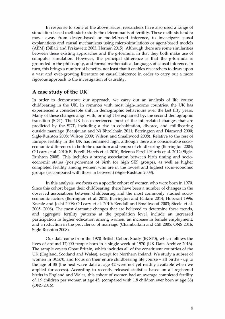
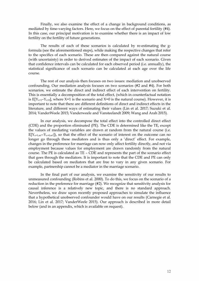
In the first instance, we generate a confounder that increases the odds of marriage in any year by 2.9 and the odds childbirth in any year by 1.5. These odds are based on its inclusion in the multivariate models for marriage and childbirth, when added as a baseline control. By comparing this to our analysis of conditional associations, including the conditional models that are run as part of the g-formula (see table 2), this appears to be a strong confounder because the only variable that has an equivalently strong association with either births or marriage is the partnership variable.

21

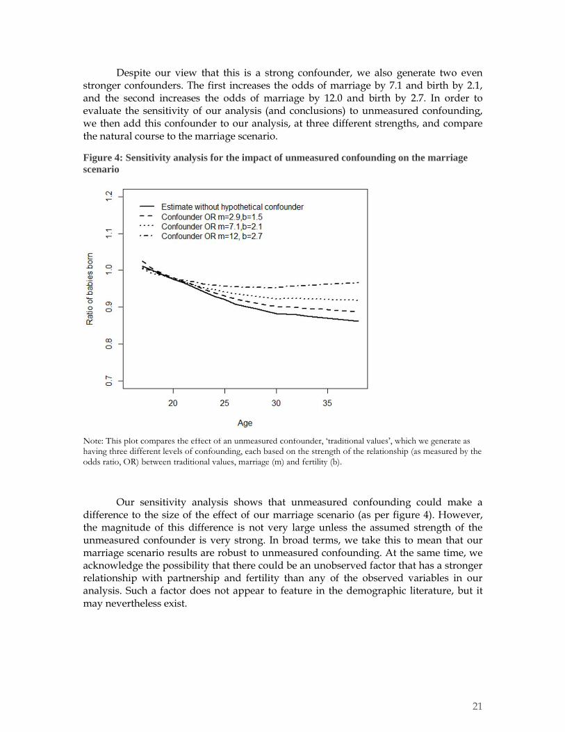
Despite our view that this is a strong confounder, we also generate two even stronger confounders. The first increases the odds of marriage by 7.1 and birth by 2.1, and the second increases the odds of marriage by 12.0 and birth by 2.7. In order to evaluate the sensitivity of our analysis (and conclusions) to unmeasured confounding, we then add this confounder to our analysis, at three different strengths, and compare the natural course to the marriage scenario.

Figure 4: Sensitivity analysis for the impact of unmeasured confounding on the marriage

scenario

Note: This plot compares the effect of an unmeasured confounder, ‘traditional values’, which we generate as having three different levels of confounding, each based on the strength of the relationship (as measured by the odds ratio, OR) between traditional values, marriage (m) and fertility (b).

Our sensitivity analysis shows that unmeasured confounding could make a difference to the size of the effect of our marriage scenario (as per figure 4). However, the magnitude of this difference is not very large unless the assumed strength of the unmeasured confounder is very strong. In broad terms, we take this to mean that our marriage scenario results are robust to unmeasured confounding. At the same time, we acknowledge the possibility that there could be an unobserved factor that has a stronger relationship with partnership and fertility than any of the observed variables in our analysis. Such a factor does not appear to feature in the demographic literature, but it may nevertheless exist.

22

Discussion

In this paper, we have demonstrated a new approach for studying the socio-economic determinants of fertility over the life course. Using a case study of women born in the UK in 1970, we have examined the influence of education, partnership, employment, and parental fertility, on childbearing at all ages from 16 to 38. Our results show that all of these factors may have a significant impact on fertility, but to different degrees, and with different profiles over the life course. In essence, the results are dependent upon the size and nature of the hypothetical effect that we consider.

The derivation of scenarios is an explicit component of our approach, and is a potential advantage because it provides a link between causal inference and generalization. On the one hand, each scenario specifies the counterfactual that is being evaluated. At the same time, each scenario can be qualitatively appraised with respect to its relevance, realism, and utility for generalization. For example, the employment scenario may be useful and relevant for policy-makers, but somewhat unrealistic because it is hard to imagine all (non-disabled) women being full-time employed one year after birth. In this sense, each scenario implicitly incorporates the ‘effect size’ of a counterfactual. For this research, we have chosen a set of scenarios that demonstrate our approach, but future research may choose to investigate whether specific scenarios are sensitive to different specifications.

In addition to total effects, such as those estimated using other causal inference approaches (like instrumental variables), the g-formula enables the analysis of time-varying mediation. We calculate direct and indirect effects for two scenarios: a reduction in the preference for marriage, and the impact of all women becoming only-children. In both scenarios, the direct effect is much larger than the indirect effect at all ages, in particular in early reproductive years. Nevertheless, our analysis suggests that mediation is far from negligible in determining the intergenerational transmission of fertility.

In the final stage of our analysis we examine the sensitivity of our results to unmeasured confounding. This is particularly important because it addresses one of the main assumptions of our approach, namely that the most important sources of confounding are observed. In practice, there may be some confounders that are not included in our analysis, but the essential question is whether they would make a difference to our findings. Based on our sensitivity analysis for the marriage scenario, they would not. However, we recognize that this is neither the only scenario, nor the only possible way of specifying unmeasured confounding. As with all research on the determinants of fertility, this is one reason why we should be cautious about stating that these relationships are definitive, or proven. Future research may therefore choose to scrutinize these findings, including with an increased emphasis on sources of bias due to the unmeasured confounding of population-averaged effects.

Added to this, unmeasured confounding is not the only limitation of our analysis. In common with many previous studies, our analysis was limited to only those women who had complete data for all variables at baseline and in the first year of observation. After that, women were censored, for the rest of the study, if they were

23

missing any variables in a given year. Given these constraints, our analysis is susceptible to assumptions regarding missing data, including that cases are missing conditionally at random (MAR) and that censoring is non-informative. Although we have no reason to believe that this would have a material impact on our findings, further research would be required in order to ascertain this with any certainty.

Another limitation, or caveat, concerns the interpretation of our results. Like most causal inference methods, the results of the g-formula are driven by observed relationships in the empirical data. For example, we show a significant impact of changes in marriage behavior on fertility behavior. However, we do not model a change in the underlying meaning of marriage. Similarly, our post-birth employment scenario does not include the anticipation of full-time employment after birth that would accompany any real-world policy to encourage such behavior. We note that this limitation is impossible to mitigate using a different method, but instead requires different data, for example data on (trial) policies that are implemented in the real world. In fact, the g-formula is a very useful method for policy evaluation, not least because it enables the examination of non-compliance and time-varying policy-uptake, which are both related to mediation. Future research might therefore choose to use the g-formula to examine the impact of policies on fertility.

There are a range of potential extensions to this method that could be undertaken in future research. A straightforward extension would be to extend the analysis to compare and contrast different subgroups, for example to compare the impact of a scenario, or its direct and indirect effects, for women who live in different regions. We could also make our scenarios more nuanced, for example to model the impact of targeted policies, or to analyze the combined effect of multiple scenarios. Our analysis has focused on women, as is almost always the case in demographic research on fertility, but could also be repeated for men.

Considering more complex extensions, it may be possible to model the fertility process, and its determinants, with greater complexity and nuance. For example, we could add more complex dependencies over time, such as causal links between determinants in one year and fertility two (or more) years later (similar to a time series analysis of AR2, AR3, etc.). The outcome, births, could also be modelled with greater nuance, for example by including stillbirths and conceptions not resulting in pregnancy. Although data are often not available, it would be interesting to incorporate the effect of abortions, miscarriages, adoptions, and child mortality. At the moment, all of these factors are absorbed into the time-varying mediating processes. Related to this, the direct effects that we model (i.e. individual pathways) could be further decomposed by examining mediation in more detail. For example, the direct effect of marriage on fertility could be explained (but not confounded) by the proximate determinants of fertility. Several other topics that we recommend for future research are to investigate the possibility of further control for unobserved heterogeneity and to examine the extent to which the findings shown here can be generalized over time (to other UK birth cohorts) or across space (to other countries). Finally, it would be possible to design a range of studies that compared the g-formula to other methods that have been used to examine the determinants of fertility.

24

In summary, we believe that this study demonstrates the benefits of a new approach – based on the parametric g-formula – for studying the socio-economic determinants of fertility. Our analysis also indicates that there may be potential benefits of using a similar approach to study similar topics in life course research. For example, the g-formula could be usefully applied to the study of linked couple-level decision-making based on individual-level data. Such analysis is often prevented, or at least made difficult, because of the simultaneity and (mediating) interrelationships between the life courses of both partners. Along similar lines, this approach could be used to study migration, which is a mediating process in the life course of most individuals.

Acknowledgements

Maarten and Ben would also like to thank the many colleagues who provided helpful comments in the development of this research. This includes the organisers and attendees of the IUSSP International Seminar on Causal Mediation Analysis in Health and Work in September 2016. Ben is grateful for financial support received from the Swedish Research Council (Vetenskapsrådet) via the Swedish Initiative for Research on Microdata in the Social and Medical Sciences (SIMSAM), grant 340-2013-5164, and from the Strategic Research Council of the Academy of Finland, decision number 293103, for the research consortium Tackling Inequality in Time of Austerity (TITA), as well as the support of the Department of Methodology at the London School of Economics. Finally, we thank Joshua Perleberg for the initial data management.

25

References

Aksoy, O., & Billari, F. C. (2015). Political Islam, marriage, and fertility: Evidence from a natural experiment in Turkey. Nuffield College, Oxford.

Andersson, G. (2004). Childbearing after Migration: Fertility Patterns of Foreign-born Women in Sweden. International Migration Review, 38(2), 747–774.

Angrist, J. D., & Pischke, J.-S. (2008). Mostly harmless econometrics: An empiricist’s companion. Princeton University Press.

Balbo, N., Billari, F. C., & Mills, M. (2012). Fertility in Advanced Societies: A Review of Research. European Journal of Population/Revue européenne de Démographie, 1–38.

Beaujouan, É., & Ní Bhrolcháin, M. (2011). Cohabitation and marriage in Britain since the 1970s. Population Trends, 145, 35–59.

Becker, G. S. (1981). A Treatise on the Family. Cambridge: Harvard University Press.

Becker, G. S., Duesenberry, J. S., & Okun, B. (1960). An economic analysis of fertility. Columbia University Press.

Berrington, A. (2004). Perpetual postponers? Women’s, men’s and couple’s fertility intentions and subsequent fertility behaviour. Population Trends, 117, 9–19.

Berrington, A., & Diamond, I. (2000). Marriage or cohabitation: a competing risks analysis of first‐ partnership formation among the 1958 British birth cohort. Journal of the Royal Statistical Society: Series A (Statistics in Society), 163(2), 127–151. doi:10.1111/1467-985X.00162

Berrington, A., & Pattaro, S. (2014). Educational differences in fertility desires, intentions and behaviour: A life course perspective. Advances in Life Course Research, 21, 10–27. doi:10.1016/j.alcr.2013.12.003

Berrington, A., Stone, J., & Beaujouan, E. (2015). Educational differences in timing and quantum of childbearing in Britain: A study of cohorts born 1940−1969. Demographic Research, 33, 733–764. doi:10.4054/DemRes.2015.33.26

Billari, F. C. (2015). Integrating macro- and micro-level approaches in the explanation of population change. Population Studies, 69(sup1), S11–S20. doi:10.1080/00324728.2015.1009712

Billari, F. C., & Galasso, V. (2009). What Explains Fertility? Evidence from Italian Pension Reforms (SSRN Scholarly Paper No. ID 1406946). Rochester, NY: Social Science Research Network. https://papers.ssrn.com/abstract=1406946. Accessed 2 April 2017

Billari, F. C., & Kohler, H.-P. (2004). Patterns of low and lowest-low fertility in Europe. Population Studies, 58(2), 161–176. doi:10.1080/0032472042000213695

Billari, F. C., & Prskawetz, A. (Eds.). (2003). Agent-Based Computational Demography. Heidelberg: Physica-Verlag HD. doi:10.1007/978-3-7908-2715-6

Buhr, P., & Huinink, J. (2014). Fertility analysis from a life course perspective. Advances in Life Course Research, 21, 1–9. doi:10.1016/j.alcr.2014.04.001

Carnegie, N. B., Harada, M., & Hill, J. L. (2016). Assessing Sensitivity to Unmeasured Confounding Using a Simulated Potential Confounder. Journal of Research on Educational Effectiveness, 9(3), 395–420. doi:10.1080/19345747.2015.1078862

Chamberlain, J., & Gill, B. (2005). Fertility and mortality. In Focus on people and migration (pp. 71–89). Springer. http://link.springer.com/chapter/10.1007/978-1-349-75096-2_5. Accessed 3 April 2017

26

Clarke, P. S., Crawford, C., Steele, F., & Vignoles, A. (2010). The Choice Between Fixed and Random Effects Models: Some Considerations for Educational Research (SSRN Scholarly Paper No. ID 1700456). Rochester, NY: Social Science Research Network. http://papers.ssrn.com/abstract=1700456. Accessed 8 May 2013

Clarke, P. S., & Windmeijer, F. (2012). Instrumental Variable Estimators for Binary Outcomes. Journal of the American Statistical Association, 107(500), 1638–1652. doi:10.1080/01621459.2012.734171

Cleland, J., & Wilson, C. (1987). Demand Theories of the Fertility Transition: An Iconoclastic View. Population Studies, 41(1), 5–30. doi:10.1080/0032472031000142516

Coale, A. J., & Watkins, S. C. (1986). The Decline of Fertility in Europe: The Revised Proceedings of a Conference on the Princeton European Fertility Project. Princeton University Press.

Daniel, R. M., Cousens, S. N., De Stavola, B. L., Kenward, M. G., & Sterne, J. A. C. (2013). Methods for dealing with time-dependent confounding. Statistics in Medicine, 32(9), 1584–1618. doi:10.1002/sim.5686

Davis, K., & Blake, J. (1956). Social Structure and Fertility: An Analytic Framework. Economic Development and Cultural Change, 4(3), 211–235.

Doll, R. (2002). Proof of causality: deduction from epidemiological observation. Perspectives in biology and medicine, 45(4), 499–515.

Dribe, M., Oris, M., & Pozzi, L. (2014). Socioeconomic status and fertility before, during, and after the demographic transition: An introduction. Demographic Research, 31, 161–182. doi:10.4054/DemRes.2014.31.7

Duclos, E., Lefebvre, P., & Merrigan, P. (2001). A “natural experiment” on the economics of storks: evidence on the impact of differential family policy on fertility rates in Canada (No. Working Paper No. 136). Center for Research on Economic Fluctuations and Employment (CREFE). http://citeseerx.ist.psu.edu/viewdoc/download?doi=10.1.1.200.8393&rep=rep1&type=pdf. Accessed 2 April 2017

Easterlin, R. A., & Crimmins, E. M. (1985). The Fertility Revolution: A Supply-Demand Analysis. University of Chicago Press.

Engelhardt, H., Kohler, H.-P., & Prskawetz, A. (2009). Causal analysis in population studies: concepts, methods, applications. Springer.

Forste, R., & Tienda, M. (1996). What’s Behind Racial and Ethnic Fertility Differentials? Population and Development Review, 22, 109–133. doi:10.2307/2808008

Gardiner, J. C., Luo, Z., & Roman, L. A. (2009). Fixed effects, random effects and GEE: What are the differences? Statistics in Medicine, 28(2), 221–239. doi:10.1002/sim.3478

Glymour, M. M. (2006). Chapter 16: Using causal diagrams to understand common problems in social epidemiology. In J. M. Oakes & J. S. Kaufman (Eds.), Methods in social epidemiology (1st ed., pp. 387–422). San Francisco, CA: Jossey-Bass.

Goisis, A., & Sigle-Rushton, W. (2014). Childbearing Postponement and Child Well-being: A Complex and Varied Relationship? Demography, 51(5), 1821–1841. doi:10.1007/s13524-014-0335-4

Greenland, S., Pearl, J., & Robins, J. M. (1999). Causal diagrams for epidemiologic research. Epidemiology, 37–48.

Hernán, M. A. (2015). Invited Commentary: Agent-Based Models for Causal Inference—Reweighting Data and Theory in Epidemiology. American Journal of Epidemiology, 181(2), 103–105. doi:10.1093/aje/kwu272

Hernán, M. A., Alonso, A., Logan, R., Grodstein, F., Michels, K. B., Willett, W. C., et al. (2008). Observational Studies Analyzed Like Randomized Experiments: An Application to

27

Postmenopausal Hormone Therapy and Coronary Heart Disease. Epidemiology, 19(6), 766–779. doi:10.1097/EDE.0b013e3181875e61

Hernán, M. A., & Robins, J. M. (2006a). Estimating causal effects from epidemiological data. Journal of Epidemiology and Community Health, 60(7), 578–586. doi:10.1136/jech.2004.029496

Hernán, M. A., & Robins, J. M. (2006b). Instruments for causal inference: an epidemiologist’s dream? Epidemiology (Cambridge, Mass.), 17(4), 360–372. doi:10.1097/01.ede.0000222409.00878.37

Hirschman, C. (1994). Why Fertility Changes. Annual Review of Sociology, 20, 203–233.

Hobcraft, J. (1996). Fertility in England and Wales: A Fifty-Year Perspective. Population Studies, 50(3), 485–524. doi:10.1080/0032472031000149586

Holland, P. W. (1986). Statistics and Causal Inference. Journal of the American Statistical Association, 81(396), 945–960. doi:10.2307/2289064

Huinink, J., & Kohli, M. (2014). A life-course approach to fertility. Demographic Research, 30, 1293–1326. doi:10.4054/DemRes.2014.30.45

Imai, K., Keele, L., & Yamamoto, T. (2010). Identification, Inference and Sensitivity Analysis for Causal Mediation Effects. Statistical Science, 25(1), 51–71. doi:10.1214/10-STS321

Imbens, G. W., & Rubin, D. B. (2015). Causal Inference for Statistics, Social, and Biomedical Sciences: An Introduction (1 edition.). New York: Cambridge University Press.

Johnson-Hanks, J., Bachrach, C. A., Morgan, S. P., & Kohler, H.-P. (2011). Understanding family change and variation : toward a theory of conjunctural action. Dordrecht; New York: Springer.

Keil, A. P., Edwards, J. K., Richardson, D. R., Naimi, A. I., & Cole, S. R. (2014). The parametric G-formula for time-to-event data: towards intuition with a worked example. Epidemiology (Cambridge, Mass.), 25(6), 889–897. doi:10.1097/EDE.0000000000000160

Khandker, S., B. Koolwal, G., & Samad, H. (2009). Handbook on Impact Evaluation: Quantitative Methods and Practices. The World Bank. http://elibrary.worldbank.org/doi/book/10.1596/978-0-8213-8028-4. Accessed 23 December 2016

Kneale, D., & Joshi, H. (2008). Postponement and childlessness - Evidence from two British cohorts. Demographic Research, 19, 1935–1968. doi:10.4054/DemRes.2008.19.58

Kuczynski, R. R. (1932). Fertility and reproduction. Falcon Press.

Kulu, H., & González-Ferrer, A. (2014). Family Dynamics Among Immigrants and Their Descendants in Europe: Current Research and Opportunities. European Journal of Population, 30(4), 411–435. doi:10.1007/s10680-014-9322-0

Kulu, H., & Steele, F. (2013). Interrelationships Between Childbearing and Housing Transitions in the Family Life Course. Demography, 50(5), 1687–1714. doi:10.1007/s13524-013-0216-2

Kulu, H., & Washbrook, E. (2014). Residential context, migration and fertility in a modern urban society. Advances in Life Course Research, 21, 168–182. doi:10.1016/j.alcr.2014.01.001

Lavy, V., & Zablotsky, A. (2011). Mother’s schooling and fertility under low female labor force participation: evidence from a natural experiment. National Bureau of Economic Research. http://www.nber.org/papers/w16856. Accessed 6 June 2016

Lee, R., & Mason, A. (2010). Fertility, Human Capital, and Economic Growth over the Demographic Transition. European Journal of Population / Revue européenne de Démographie, 26(2), 159–182. doi:10.1007/s10680-009-9186-x

Lesthaeghe, R. (1983). A Century of Demographic and Cultural Change in Western Europe: An Exploration of Underlying Dimensions. Population and Development Review, 9(3), 411–435. doi:10.2307/1973316

28

Lesthaeghe, R. (2010). The unfolding story of the second demographic transition. Population and development review, 36(2), 211–251.

Lin, S.-H., Young, J., Logan, R., Tchetgen Tchetgen, E. J., & VanderWeele, T. J. (2017). Parametric Mediational g-Formula Approach to Mediation Analysis with Time-varying Exposures, Mediators, and Confounders: Epidemiology, 28(2), 266–274. doi:10.1097/EDE.0000000000000609

Lorimer, F. (1956). Culture and Human Fertility. Journal of School Health, 26(4), 136–136. doi:10.1111/j.1746-1561.1956.tb00823.x

McCrary, J., & Royer, H. (2011). The Effect of Female Education on Fertility and Infant Health: Evidence from School Entry Policies Using Exact Date of Birth. American Economic Review, 101(1), 158–195. doi:10.1257/aer.101.1.158

Mclanahan, S. (2004). Diverging destinies: How children are faring under the second demographic transition. Demography, 41(4), 607–627. doi:10.1353/dem.2004.0033

Milewski, N. (2010). Fertility of Immigrants: A two-generational approach in Germany. Berlin, Heidelberg: Springer Berlin Heidelberg. http://link.springer.com/10.1007/978-3-642-03705-4. Accessed 19 January 2017

Moffitt, R. (2003). Causal analysis in population research: An economist’s perspective. Population and Development Review, 29(3), 448–458.

Moffitt, R. (2005). Remarks on the Analysis of Causal Relationships in Population Research. Demography, 42(1), 91–108.

Monstad, K., Propper, C., & Salvanes, K. G. (2008). Education and Fertility: Evidence from a Natural Experiment*. Scandinavian Journal of Economics, 110(4), 827–852. doi:10.1111/j.1467-9442.2008.00563.x

Morgan, S. L., & Winship, C. (2007). Counterfactuals and causal inference: methods and principles for social research. New York: Cambridge University Press.

Myrskyla, M., Kohler, H.-P., & Billari, F. C. (2009). Advances in development reverse fertility declines. Nature, 460(7256), 741–743. doi:10.1038/nature08230

Neyer, G., Lappegård, T., & Vignoli, D. (2013). Gender Equality and Fertility: Which Equality Matters? European Journal of Population / Revue européenne de Démographie, 29(3), 245–272. doi:10.1007/s10680-013-9292-7

Ní Bhrolcháin, M., & Dyson, T. (2007). On Causation in Demography: Issues and Illustrations. Population and Development Review, 33(1), 1–36.

Nisén, J., Myrskylä, M., Silventoinen, K., & Martikainen, P. (2014). Effect of family background on the educational gradient in lifetime fertility of Finnish women born 1940–50. Population Studies, 68(3), 321–337. doi:10.1080/00324728.2014.913807

O’Leary, L., Natamba, E., Jefferies, J., & Wilson, B. (2010). Fertility and partnership status in the last two decades. Population Trends, 140, 5–35.

ONS. (2016). Childbearing for women born in different years, England and Wales: 2015 (published online). Office for National Statistics. https://www.ons.gov.uk/peoplepopulationandcommunity/birthsdeathsandmarriages/conceptionandfertilityrates/bulletins/childbearingforwomenbornindifferentyearsenglandandwales/2015/pdf. Accessed 3 April 2017

Pearl, J. (1995). Causal Diagrams for Empirical Research. Biometrika, 82(4), 669–688. doi:10.2307/2337329

Pearl, J. (2009). Causality: Models, Reasoning and Inference (2nd Revised edition.). Cambridge University Press.

29

Perelli-Harris, B., Kreyenfeld, M., Sigle-Rushton, W., Keizer, R., Lappegård, T., Jasilioniene, A., et al. (2012). Changes in union status during the transition to parenthood in eleven European countries, 1970s to early 2000s. Population Studies, 66(2), 167–182. doi:10.1080/00324728.2012.673004

Perelli-Harris, B., Sigle-Rushton, W., Kreyenfeld, M., Lappegård, T., Keizer, R., & Berghammer, C. (2010). The educational gradient of childbearing within cohabitation in Europe. Population and development review, 36(4), 775–801.

Rendall, M. S., & Smallwood, S. (2003). Higher qualifications, first-birth timing and further childbearing in England and Wales. Population Trends, 111, 18–26.

Robins, J. M. (1986). A new approach to causal inference in mortality studies with a sustained exposure period—application to control of the healthy worker survivor effect. Mathematical Modelling, 7(9–12), 1393–1512. doi:10.1016/0270-0255(86)90088-6

Robins, J. M., & Hernán, M. A. (2009). Chapter 23: Estimation of the causal effects of time-varying exposures. In Longitudinal data analysis (pp. 553–599). Chapman & Hall/CRC.

Robins, J. M., Rotnitzky, A., & Scharfstein, D. O. (2000). Sensitivity Analysis for Selection bias and unmeasured Confounding in missing Data and Causal inference models. In Statistical Models in Epidemiology, the Environment, and Clinical Trials (pp. 1–94). Springer, New York, NY. doi:10.1007/978-1-4612-1284-3_1

Rubin, D. B. (1974). Estimating causal effects of treatments in randomized and nonrandomized studies. Journal of educational Psychology, 66(5), 688.

Sampson, R. J., Winship, C., & Knight, C. (2013). Translating Causal Claims: Principles and Strategies for Policy-Relevant Criminology. Criminology & Public Policy, 12(4), 587–616. doi:10.1111/1745-9133.12027

Sigle-Rushton, W. (2008). England and Wales: Stable fertility and pronounced social status differences. Demographic research, 19(15), 455–502.

Smith, H. L. (2009). Causation and Its Discontents. In H. Engelhardt, H.-P. Kohler, & A. Prskawetz (Eds.), Causal analysis in population studies: concepts, methods, applications. Springer. http://books.google.co.uk/books/about/Causal_Analysis_in_Population_Studies.html?id=ArfD-y8lvaQC

Steele, F., Joshi, H., Kallis, C., & Goldstein, H. (2006). Changing compatibility of cohabitation and childbearing between young British women born in 1958 and 1970. Population Studies, 60(2), 137–152. doi:10.1080/00324720600598009

Steele, F., Kallis, C., Goldstein, H., & Joshi, H. (2005). The relationship between childbearing and transitions from marriage and cohabitation in Britain. Demography, 42(4), 647–673.

Suzuki, E., Mitsuhashi, T., Tsuda, T., & Yamamoto, E. (2014). Alternative Definitions of “Proportion Eliminated”: Epidemiology, 25(2), 308–309. doi:10.1097/EDE.0000000000000050

Tropf, F. C., & Mandemakers, J. J. (2017). Is the Association Between Education and Fertility Postponement Causal? The Role of Family Background Factors. Demography, 54(1), 71–91. doi:10.1007/s13524-016-0531-5

UK Data Archive. (2016). 1970 British Cohort Study. University of Essex, Institute for Social and Economic Research.

van de Kaa, D. J. (1987). Europe’s Second Demographic Transition. Population Bulletin, 42(1). Accessed 16 August 2014

VanderWeele, T. J. (2015). Explanation in Causal Inference: Methods for Mediation and Interaction (1 edition.). New York: Oxford University Press.

30

Vanderweele, T. J., & Vansteelandt, S. (2009). Conceptual issues concerning mediation, interventions and composition. Statistics and Its Interface, 2(4), 457–468. doi:10.4310/SII.2009.v2.n4.a7

Vansteelandt, S. (2012). Understanding Counterfactual-Based Mediation Analysis Approaches and Their Differences: Epidemiology, 23(6), 889–891. doi:10.1097/EDE.0b013e31826d0f6f

Wang, A., & Arah, O. A. (2015). G-computation demonstration in causal mediation analysis. European Journal of Epidemiology, 30(10), 1119–1127. doi:10.1007/s10654-015-0100-z

Wilson, B. (2009). Estimating the cohabiting population. Population Trends, 136, 21–27.

Wilson, B., & Smallwood, S. (2008). The proportion of marriages ending in divorce. Population Trends, 131, 28.