a natural nonparametric generalization of parametric...

A Natural Nonparametric Generalization of Parametric

Statistical Models

Tim Hanson

Division of Biostatistics

University of Minnesota

November, 2008

1

• To Bayes or not to Bayes...

• The Polya tree prior.

• Applications: mixed models and survival analysis.

– Meta analysis.

– Generalized linear mixed models with exchangeable and

partially exchangeable random effects.

– Multivariate Polya trees.

2

Why Bayes?

• Incorporation of existing prior information.

• Through MCMC, able to fit models cannot fit otherwise.

• Complex, multi-level nested and/or crossed GLMMs relatively

painless to fit. Approximations at level of likelihood not

necessary.

Why not Bayes?

• Subjective? Choosing a model is subjective!

• Computationally intensive.

• Lack of easy to use software? Not anymore: WinBUGS & brugs,

DPpackage (and many more) for R, SAS proc mcmc, BayesX,

more...

3

Bayesian nonparametrics

• Why? One word: flexibility.

• Improved prediction, more realistic models.

• Several priors to choose from: Dirichlet process and other stick

breaking processes (Pitman-Yor, species sampling, etc.),

normalized inverse Gaussian, beta, gamma, extended (smoothed)

versions, Polya trees, Bernstein polynomials, wavelets, penalized

splines, etc.

• For distributional modeling, take prior on space of all probability

distributions.

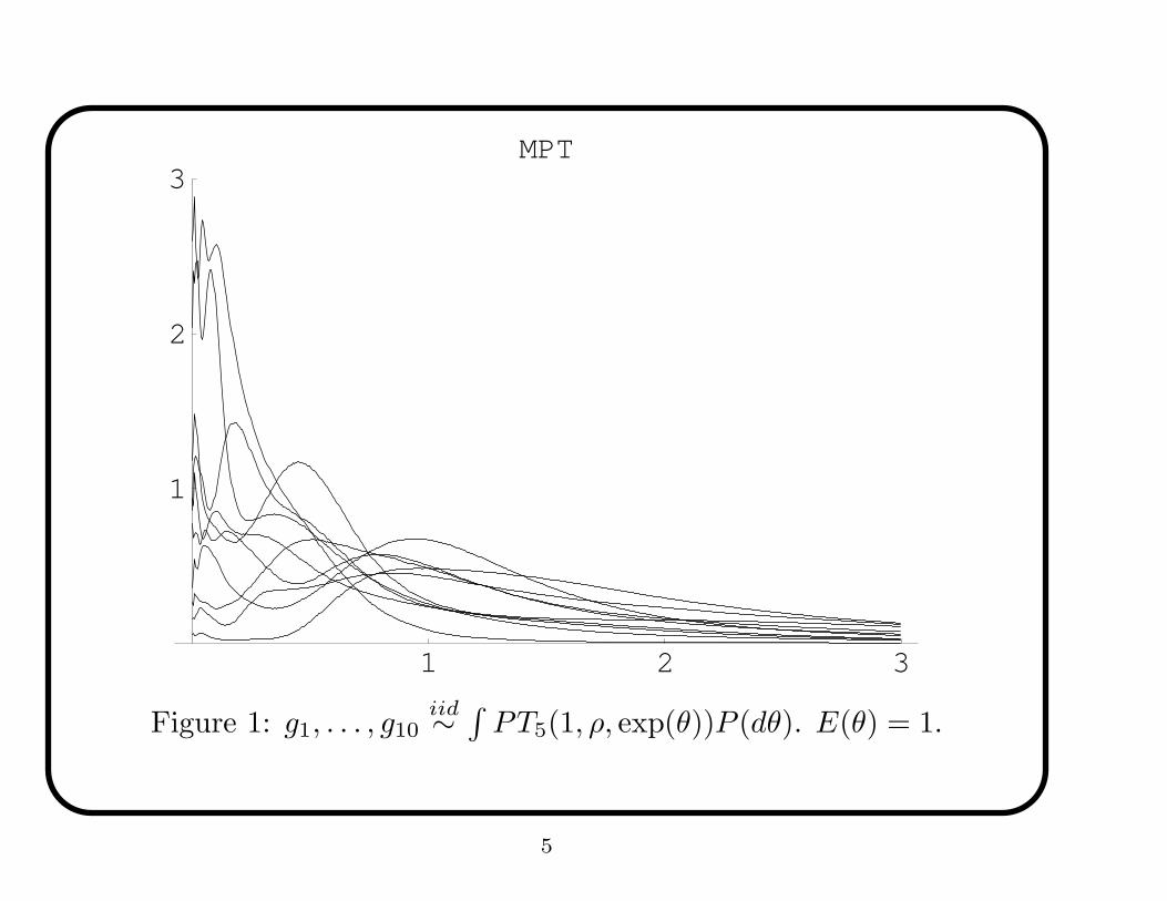
• Example: On next slide is 10 iid random densities from a mixture

of Polya trees (MPT) prior centered at the exp(1) distribution...

4

1 2 3

1

2

3MPT

Figure 1: g1, . . . , g10iid∼

∫

PT5(1, ρ, exp(θ))P (dθ). E(θ) = 1.

5

Polya trees generalize existingparametric families

• Can add parameters Y0, Y00, Y10, Y000, Y010, Y100, Y110to (µ, σ2) to make N(µ, σ2) more flexible.

6

Univariate Polya tree prior

• Notation: G ∼ PT (c, ρ(·), Gθ). G is random probability measure

centered at Gθ, parametric on R.

• Polya tree prior is tail-free (Freedman, 1963); Dirichlet process

special case ρ(j) = 2−j .

• History of Polya tree dates to 60’s & 70’s. Early work

summarized in Ferguson (1974).

• Mauldin, Sudderth, & Williams (1992) and Lavine (1992, 1994)

develop more theory.

• Walker and Mallick (1997, 1999), Walker et al. (1999) use Polya

trees in GLMM and survival models. Inference via MCMC.

7

Polya tree = partition + conditional probabilities

• Polya tree prior on G defined through nested partitions of R, say

Πθj , and associated conditional probabilities Yj at level j.

– Finite tree has j ≤ J .

– On level J sets G follows Gθ.

– Rule of thumb: J ≤ log2 n.

• Partition Πθj at level j splits R into 2j pieces of equal probability

under Gθ. Sets denoted Bθ(ε) where ε is binary.

• Next slide shows Π1, Π2, and Π3 for Gθ = N(0, 1).

8

-1 1

000 111001 110010 001011 100

00 1101 10

0 1

Figure 2: First 3 partitions of R generated by N(0, 1).

9

• Parametric Gθ gives partition.

• Add Y1 = Y0, Y1, Y2 = Y00, Y01, Y10, Y11,Y3 = Y000, Y001, Y010, Y011, Y100, Y101, Y110, Y111, etc. to refine

density shape. Let Y = Y1,Y2, . . . ,YJ.

• Yε0 = GBθ(ε0)|Bθ(ε). Yε1 = 1 − Yε0.

• Next slide uses Gθ = Weibull(2, 10).

– Upper left: all Yε = 0.5 gives back Weibull(2, 10).

– Upper right: (Y0, Y1) = (0.45, 0.55).

– Middle left: adds (Y00, Y01) = (0.4, 0.6), (Y10, Y11) = (0.6, 0.4).

– Middle right: Y000 = 0.3, Y010 = 0.3, Y100 = 0.6, Y110 = 0.3.

– Lower right: Keeping Y as above but mixing over Weibull

parameters.

10

2 4 6

0.2

0.4

2 4 6

0.2

0.4

1.7 2.6 3.7

0.2

0.4

1.2 1.7 2.2 2.6 3.1 3.7 4.6

0.2

0.4

2 4 6

0.2

0.4

2.6

0.2

0.4

Figure 3: J = 0, 1, 2, 3 for Weibull(2,10).

11

Prior on (Yε0, Yε1)

• Want E(Yε0) = 0.5 to center G at Gθ. Take

Yε0 ∼ beta(cρ(j), cρ(j)).

• c and ρ(j) affect how quickly data “take over” parametric

centering family Gθ : θ ∈ Θ.

• c is overall weight attached to Gθ. ρ(j) affects how “clumped”

data are. ρ(j) = j2 often used.

• Have EG(A) = Gθ(A). varG(A) depends on overall weight c

and function ρ(·).

12

“Standard” parameterization where ρ(j) = j2:

R

B0 B1

(Y0, Y1) ∼ Dir(c, c)

B00 B01 B10 B11

(Y00, Y01) ∼ Dir(4c, 4c) (Y10, Y11) ∼ Dir(4c, 4c)

B000 B001 B010 B011 B100 B101 B110 B111

(Y000, Y001) ∼

Dir(9c, 9c)

(Y010, Y011) ∼

Dir(9c, 9c)

(Y100, Y101) ∼

Dir(9c, 9c)

(Y110, Y111) ∼

Dir(9c, 9c)

Π1 = B0, B1, Y1 = Y0, Y1.

Π2 = B00, B01, B10, B11, Y2 = Y00, Y01, Y10, Y11.

Π3 = B000, B001, B010, B011, B100, B101, B110, B111

Y3 = Y000, Y001, Y010, Y011, Y100, Y101, Y110, Y111

Adds 7 free parameters Y = Y0, Y00, Y10, Y000, Y010, Y100, Y110.

13

Mixtures of Polya trees:

• MPT considered by Lavine (1992), Berger and Guglielmi (2001),

Hanson and Johnson (2002), Hanson (2006), etc.

• Further taking θ ∼ p(θ) induces MPT; somewhat smooths out

partitioning effects of PT.

• MCMC can be straightforward to set up based on underlying

parametric model, but mixing is poor if underlying model grossly

incorrect.

• Ongoing research: adaptive MCMC for MPT models.

• Next slide shows highly non-normal data and MPT estimate.

BF ≈ 1010 in favor of MPT vs. N(µ, σ2).

14

10 20 30 40

0.05

0.1

0.15

Figure 4: Galaxy data: x1, . . . , x82|G ∼ G, G ∼ PT5(c, ρ, N(µ, σ2)).

Solid is c ∼ Γ(5, 1), long-dashed is c = 0.1, short-dashed is Gaussian

kernel-smoothed, h = 1.

15

10 20 30 40 50

0.005

0.01

0.015

0.02

0.025

0.03

Figure 5: ti = time to leukemia relapse; children treated w/ 6-

mercaptopurine. t1, . . . , t21|G iid∼ G, G ∼∫

PT5(1, ρ, exp(θ))p(θ)dθ

where p(θ) ∝ 1. Density estimates for c = 1 and c = ∞. Black uncen-

sored, grey censored. PBF = 0.83 for MPT vs. exp(θ), BF = 0.61.

16

Example 1:

Polya tree mixture model withapplication to meta analysis

17

Meta analysis:

• Combine summaries across multiple studies designed to address

the same scientific question.

• Observed study-specific effects y = (y1, . . . , yn);

corresponding ‘true’ effects θ = (θ1, . . . , θn).

• e.g. y vector of observed log odds ratios w/ θ corresponding

latent population LORs.

• yi approximately normal w/ mean θi via asymptotics.

• Common to use N(µ, τ2) for latent θi.

18

Normal-normal model

• For i = 1, . . . , n,

yi|θiind.∼ N(θi, σ

2i )

θi|µ, τiid∼ N(µ, τ2)

• σ2i typically fixed at estimated variance of yi.

• Normal-normal model attractive in part because µ represents

single encompassing effect measure.

• Primary statistical aim: make inferences about µ, e.g. H0 : µ > 0.

• Study-specific covariates easily added.

19

Generalize parametric normal-normal w/ MPT

• Main goal: broaden class of random effects distributions to

include the normal but allow for flexibility. Retain simplicity of

normal-normal model in terms of a unifying effect measure when

appropriate

• Get direct, robust inference for functionals other than measures

of center, which is particularly important when there is evidence

of systematic heterogeneity across studies.

• Address computational aspects of model fitting, model selection,

and nonparametric inferences for PTMs.

20

Nonparametric meta-analysis: PTM

• Generalize second level of normal-normal using

θi|G iid∼ G

where G is assigned a Polya tree prior centered on the normal

family.

yi|θiind.∼ N(θi, σ

2i )

θi|G iid∼ G

G|µ, τ, ν, c ∼ PTJ

(

c, ρν , N(µ, τ2))

(µ, τ2, ν) ∼ p(µ, τ2, ν)

where σ1, . . . , σn are fixed constants.

• µ is still the median; MPT constrained so that G(µ) = 0.5.

21

Nonparametric meta-analysis: PTM

• Prior is

µ|τ2 ∼ N(aµ, bµτ2), τ−2 ∼ Γ(aτ , bτ ), ν ∼ N(aν , bν).

• Weight c set to small constant, e.g. c = 1. Too small gives prior

mass on approximately discrete distributions ⇒ MCMC mixing

suffers to point of intractability.

• Posterior inferences for median µ and G obtained from Gibbs

sampling.

22

Nonparametric meta-analysis: DPM

• PTM model provides alternative to Dirichlet process mixture

(DPM) model.

• DPM adds flexibility by instead considering

G|µ, τ ∼ DP (α, N(µ, τ2)); i.e. a DP with fixed weight α and

prior on (µ, τ2).

• Use of a DP random effects distribution eliminates the

straightforward interpretation of µ since it no longer represents

an encompassing effect measure.

• To fix this, Burr and Doss (2005, JASA) consider a conditional

DPM in which G has median µ.

23

Polya tree mixture models

• For Polya tree priors, typically ρ(j) = j2 giving absolutely

continuous G with probability one in fully specified tree.

• Unlike previous approaches, we consider

ρν(j) = 2−νj .

Allows for spikes and clumping of probability mass; e.g. can

approximate discrete G.

• e.g. ν = 1 gives approximate DP prior; ν < 0 gives densities.

24

Model comparison

• Empirical Bayes approach coupled w/ sensitivity analysis.

c = 1, 10 & ν is fixed at a posterior estimate.

• For fixed (c, ν), a test of whether or not the underlying Gaussian

model is appropriate is carried out using the Savage-Dickey ratio.

• The normal model obtains when PT conditional probabilities are

all 0.5.

25

Model comparison

• Bayes factors.

• Also log-pseudo marginal likelihood (LPML): measure of how

well supported each observation is by the remaining data and

model, aggregated over all n observations

LPML =n

∑

i=1

log p(yi|y−i)

• Compare models using the pseudo Bayes factor, which roughly

indicates which model is superior at predicting the observed

data: PBF12 = exp(LPML1 − LPML2)

26

Simulated Data

• Data: Sample means simulated from n = 100 studies each w/ 100

individuals.

• θ1, . . . , θ100 ∼ skewed bimodal distribution ⇒ get inferences for

G since this suggests systematic heterogeneity across location.

• Model: yi|θi ∼ N(θi, σ2/100), θi ∼ G where

G ∼ PT (c, ρν, N(µ, τ2))

• Prior: µ|τ2 ∼ N(0, 1000τ2) and τ−2 ∼ Γ(0.01, 0.01). Set c = 1

and used ν = −1 for calculating BF, and ν ∼ N(0, 4) for

inference about functionals of G

• Sampled 100 simulated data sets of size 100.

• Bayes factors ranged from 105 to 1020 in favor of the PTM.

27

-10 0 10 20 30

0.05

0.1

Figure 6: Normal-normal fit & PTM refinement. Dashed = average

posterior across 100 data sets. True effects dist’n = solid line.

28

Alcohol and breast cancer

• Meta-analysis of 39 studies; mix of retrospective and prospective

designs; conducted in several countries.

• Summary measure was the estimated change in log odds ratio

(scaled as LOR × 1000) for a one gram increase in daily alcohol

consumption.

• PTM analysis: J = 5; µ|τ2 ∼ N(0, 1000τ2), τ−2 ∼ Γ(0.01, 0.01),

and ν ∼ N(0, 4). With these priors, the posterior mode of ν is

essentially 0 so we also analyzed the data and computed PBFs

with ν fixed at 0.

• PTM analysis favored over the normal-normal model with PBF

≈ 3000.

• A comparison of the conditional DPM (α = 1) versus PTM

model yielded PBF ≈ 220 in favor of the PTM.

29

-50 -25 0 25 50

0.025

0.05

Figure 7: Data-driven flexibility of the PTM apparent, especially in

the outer percentiles. Short-dashed ν ∼ N(0, 4); long-dashed ν = 0.

30

Example 2:

Cox regression with nonparametricfrailties fit in DPpackage

31

Generalized linear mixed models: generalizing Gaussian random

effects distribution

Response yij where

yij ∼ Poisson(eηij )

yij ∼ bin

(

nij ,eηij

1 + eηij

)

yij ∼ bin (nij , Φ(ηij))

P (yij = k) = Φ(αk + ηij) for k = 1, . . . , K

yij ∼ N(ηij , σ2)

yij ∼ Γ(eηij , ν)

DPpackage by Alejandro Jara implements: Poisson, logistic, probit,

cumulative probit-link for ordered categorical data, normal, and

gamma regression models with random effects. Linear predictor ηij

modeled through several Bayes NP priors...

32

Linear predictor is

ηij = x′ijβ + z′ijbi, where b1, . . . ,bm|G iid∼ G.

DPpackage can fit (among many other Bayes NP models):

• G ∼ DP (α, Gθ)

• g(x) =∫

Rd φ(x|m,Ω)dH(m) where H ∼ DP (α, Gθ)

• G ∼ PT (c, ρ(·), Gθ)

Gθ = Nd(µ,Σ). Prior placed on (µ,Σ, β). Also: Ω, σ−2, ν, α.

That is, looked at MDP, MDPM, and MPT priors on random effects

distribution G.

33

Frailty modeling in the proportional hazards model

Hazard function:

λ0(t) = limε→0

P (t ≤ T0 < t + ε|T0 ≥ t)

ε=

f0(t)

S0(t).

Conditionally proportional hazards:

λ(tij |xij) = λ0(t) exp(x′ijβ + γi).

• i = 1, . . . , n groups

• j = 1, . . . , ni within group i.

• Data (xij , tij , δij).

34

• Hazard function is piecewise constant on partition of R+.

Partition comprised of K intervals.

λ0(t) =K

∑

k=1

λkIak−1 < t ≤ ak

where a0 = 0 and aK = ∞.

• Implies Poisson likelihood

L(β, λ, γ) =n

∏

i=1

ni∏

j=1

K(tij)∏

k=1

e−ex′ijβ+γi∆ijk

[

ex′ijβ+γiλK(tij)

]δij

where ∆ijk = minak, tij − ak−1 and K(t) = maxk : ak ≤ t.

• Take K = 10 from %iles of data.

35

• Data on n = 38 kidney patients; each has ni = 2 infection times,

several right censored.

• Only covariate of interest: gender.

• Analyzed in Walker and Mallick (1997) with piecewise

exponential model and frailties following PT8(0.1, ρ, N(0, 102)).

• Poisson likelihood in form of GLMM. Fit in DPpackage:

fit2=PTglmm.default(fixed = y ~ g + h, random = ~1 | id,

family = poisson(log), offset = log(off), prior = prior2,

mcmc = mcmc2, state = state, status = FALSE)

• Assume

γ1, . . . , γn|G iid∼ G, G ∼ PT (c, ρ, N(0, σ2)), σ−2 ∼ Γ(aσ, bσ)

log λ ∼ NK(m0,V0), β ∼ Np(b0,B0), c ∼ Γ(ac, bc).

36

Bayesian semiparametric generalized linear mixed effect model

Model’s performance:

Dbar Dhat pD DIC LPML

374.45 351.09 23.37 397.82 -201.66

Regression coefficients:

Mean Median Std. Dev. Naive Std.Error 95%CI-Low 95%CI-Upp

(Intercept) -0.013506 -0.006234 0.142077 0.004493 -0.320878 0.277733

g -1.435111 -1.416729 0.482620 0.015262 -2.402870 -0.549498

h1 -4.299368 -4.259838 0.571100 0.018060 -5.509669 -3.298870

h2 -3.740145 -3.702957 0.576537 0.018232 -4.907587 -2.682208

h3 -3.907660 -3.876771 0.570570 0.018043 -5.100021 -2.861654

h4 -2.948614 -2.912574 0.573208 0.018126 -4.179309 -1.892098

h5 -3.087463 -3.046317 0.546165 0.017271 -4.138270 -2.070438

h6 -3.748874 -3.747799 0.581659 0.018394 -4.987058 -2.621747

h7 -4.597002 -4.558640 0.636655 0.020133 -5.867402 -3.480104

h8 -3.324208 -3.332950 0.602217 0.019044 -4.503470 -2.208580

h9 -3.218744 -3.234147 0.666629 0.021081 -4.549745 -1.911680

h10 -3.515208 -3.547174 0.687001 0.021725 -4.857640 -2.108612

Baseline distribution:


mu-(Intercept) 0.00000 0.00000 0.00000 0.00000 0.00000 0.00000

sigma-(Intercept) 0.65845 0.52536 0.53939 0.01706 0.15881 1.91989

Precision parameter:


alpha 0.3957673 0.3974533 0.0045467 0.0001438 0.3843464 0.4009077

Acceptance Rate for Metropolis Steps = 0.1933333 0.6004101 0 0.1512987 0.994026

37

Density of (Intercept)

values

dens

ity

−2.48 −1.90 −1.31 −0.72 −0.13 0.45 1.04 1.63

0.00

0.15

0.29

0.44

0.59

Figure 8: Estimated frailty distribution.

38

0 50 100 150 200 250 300

0.00.2

0.40.6

0.81.0

time

survi

val

Figure 9: Predictive time to infection: males.

39

0 50 100 150 200 250 300

0.20.4

0.60.8

1.0

time

survi

val

Figure 10: Predictive time to infection: females.

40

• We obtain βg = −1.4. McGilchrist and Aisbett (1991) get

βg = −1.8 w/ other covariates included. Aslanidou et al. (1995)

and Walker and Mallick (1997) get βg = −1.0.

• DIC = 398 from either MPT or normal model. Normal model

does about the same.

• MPT generalization doesn’t do harm if not needed.

41

Example 3:

Partially exchangeable randomeffects with application to Achemonkey hunting

42

• Paraguayan Ache tribe part-time hunter-gatherers; in contact

with “modern civilization” only since the mid-1970’s.

• McMillan (2001) spent year living w/ Ache collecting data.

• Part of Ache life spent on extended forest treks – only eat food

they gather or hunt. Capuchin monkeys shot out of trees.

• Hunters split into two groups, one chasing a troop of monkeys

towards the other group who shoot at them with bows and

arrows.

• Dangerous because arrows fired straight up fall back out of the

trees. Hunting prowess contributes to group status.

• Questions: how does age affect ability to hunt monkeys? How

heterogenous is hunting ability?

43

• Yij = monkeys killed by hunter i on jth trek,

i = 1, . . . , 47, j = 1, . . . , Ni.

• Mij = length in days trek ij.

• Model:

Yij |λi ∼ Pois(λiMij),

where

log λi = β0 + β1(ai − 45) + β2(ai − 45)2 + γi.

• Fixed effects (β0, β1, β2) capture overall population trend in

hunting ability due to age ai.

• Random effects γi are surrogate for “innate” hunting ability.

• Random effects commonly assumed exchangeable normal

γ1, . . . , γ47|σ ∼ N(0, σ2).

44

−4

−2

02

4

0.00 0.05 0.10 0.15 0.20 0.25

va

lue

s

density

45

• McMillan, anthropologist who spend a year w/ Ache surprised.

• Expected “clumps” of good and bad hunters based on experience.

• We see essentially Gaussian distribution of hunting ability.

• Problem: confounding between frailty distribution and hunter’s

age. Older hunters spent more time in the forest when they were

young ; younger Ache spend more time farming and playing

soccer.

• Age represents warped timescale of actual time spend hunting,

which would be better predictor. Unfortunately cannot easily

measure this.

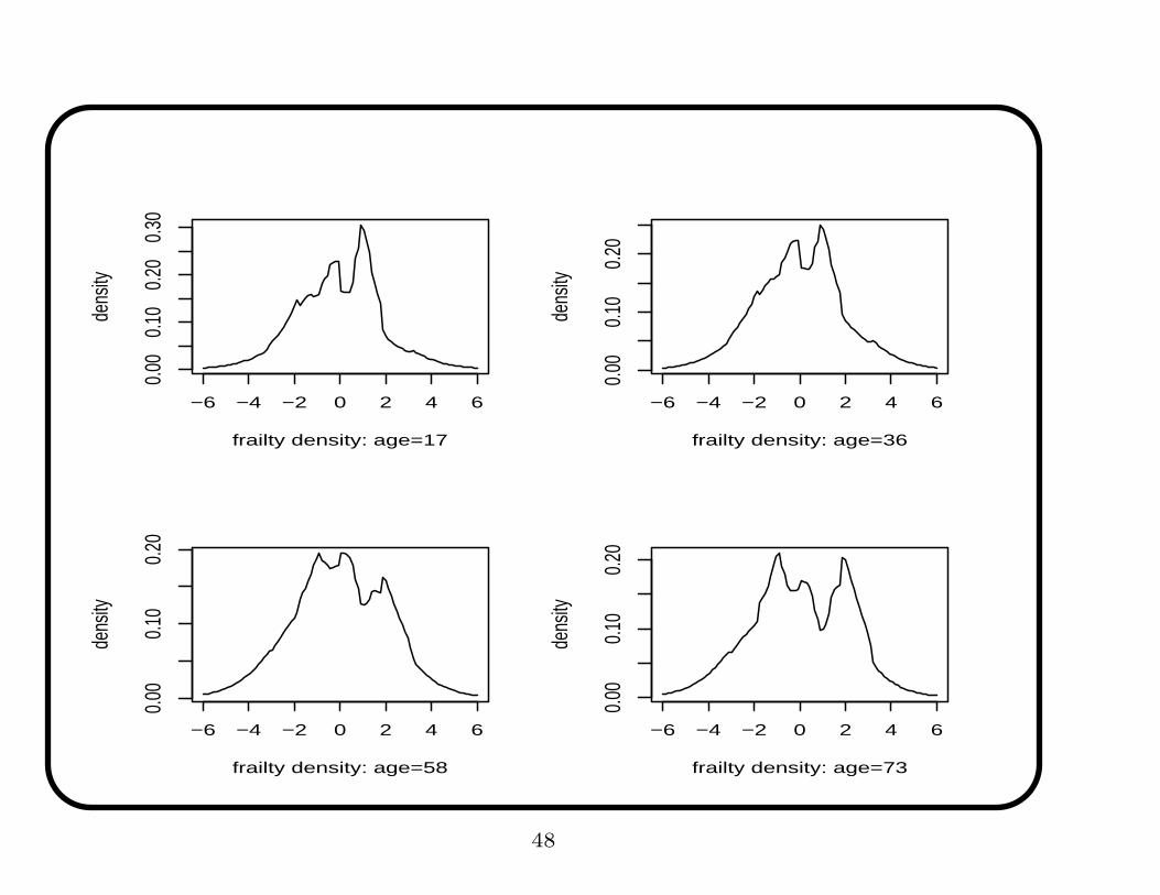
• New model γi|xi ∼ Gxiwhere Gxi

has Yε = Yε(ai).

46

Dependent Polya tree

• Basic idea is simple: replace each conditional probability w/ a

logistic regression:

Yε0(x, βε0) =exp(x′βε0)

1 + exp(x′βε0), Yε1(x, βε0) =

1

1 + exp(x′βε0).

• εθ(γ, j) is set in Πθj that γ is in.

g(γi) = 2Jφθ(γi)J

∏

i=1

Yεθ(γi,j).

• Density of random effects is

p(γ1, . . . , γn|θ, β) =

n

i=1

φθ(γi)

ε∈Ej−1

n

i=1

exp(x′iβε0)

Iγi∈Bθ(ε0)

[1 + exp(x′iβε0)]

Iγi∈Bθ(ε)

.

• Product of 2J − 2 logistic regression kernels, one for each ε0,

times parametric likelihood for θ.

47

−6 −4 −2 0 2 4 6

0.00

0.10

0.20

0.30

frailty density: age=17

dens

ity

−6 −4 −2 0 2 4 6

0.00

0.10

0.20


dens

ity

−6 −4 −2 0 2 4 6

0.00

0.10

0.20


dens

ity

−6 −4 −2 0 2 4 6

0.00

0.10

0.20


dens

ity

48

−6 −4 −2 0 2 4 6

0.00

0.05

0.10

0.15

0.20

frailty density: averaged

dens

ity

49

• Inference surprisingly easy to get: uses iteratively re-weighted

least squares M-H proposal (Gamerman, 1997).

• Evidence of confounding. Density ‘evolves’ with age. Shows more

heterogeneity and clump of ‘better’ hunters for older ages.

• Densities averaged over age looks almost identical to

exchangeable PT density!

• Dependent model provides best prediction according to LPML.

PBF ≈ 50 for DTFP vs. Gaussian.

Model LPML β0 β1 β2

N(0, σ2) −69 −2.54 0.041 −0.0061

PT (c, ρ, N(0, σ2)) −70 −2.62 0.042 −0.0057

DTFP (c, ρ, N(0, σ2)) −65 −3.00 0.058 −0.0073

50

• Will eventually be in DPpackage

fit=DTFglmm(fixed = monkeys ~ ages1 + ages2, random = ~1 | hunter,

modeltf = ~ages1, family = poisson(log), offset = log(days),

prior = prior, mcmc = mcmc, state = NULL, status = TRUE,

prediction = prediction)

• Other dependent Polya tree models use logit-transformed Gaussian

process for conditional probabilities and CAR prior giving longitudinal

and spatial dependence, respectively.

• Applications to modeling breast cancer survival from SEER data: two

Minnesota Biostat tech reports.

51

Example 4:

A bit on multivariate Polya trees

52

• Developed by Paddock (1999); Paddock et al. (2003); Hanson

(2006); Jara, Hanson, and Lesaffre (2007); Hanson, Branscum,

and Gardner (2008).

• Many ways to define partition sets Bθ(j,k). Natural,

computationally tractable approach is to consider Σ = UU′

where U comes from (a) Cholesky, (b) U = MΛ1/2, or (c)

U = MΛ1/2M′. M and Λ come from spectral decomposition.

Then consider affine transformation of “canonical” multivariate

Polya tree centered at Nd(0, I).

• Considering U = MΛ1/2O where O ∼ Haar(d) vastly smooths

inference (Jara et al., 2009).

• Too many parameters to sample Yj . Instead, we marginalize and

base inference on p(b1, . . . ,bm|µ,Σ).

53

LMM example: Carlin & Louis (2000) and Basu & Chib (2003)

look at√

CD4 counts yij for individual i at time tj , i = 1, . . . , 467,

j = 1, . . . , ni. The model for each subject is

yi = Xiβ + Zibi + εi,

where we assume

b1, . . . ,b467|G iid∼ G, G ∼∫

PT5(c, ρ, ΦΣ)dP (c,Σ),

and have the usual conjugate priors for β and ε provided in Carlin

and Louis. Prior Σ−1 ∼ Wishart(24,S0) also provided in C & L.

Long story short: (1) BF for MPT versus parametric model is greater

than 10250, (2) BF for MPT versus equivalent DPM model is greater

than 10200.

54

-5 0 5Intercept

-0.4

0

0.4

Slope

Figure 11: Predictive density level curves of G with E(bi|y1, . . . ,y467).

55

50 150 250 350Radiation

1

3

5

Ozone

50 150 250 350Radiation

1

3

5

Ozone

Figure 12: Last plot! Environmental data: U = MΛ1/2M′ (left) and

U = MΛ1/2O, O ∼ Haar(d) (right).

56

Comments...

• MPT have not been tapped to full potential.

• Often fits better than mixture of normals; especially data that

exhibit drastic change over small area. Draper (1999) notes

“wavelet-like” properties.

• If underlying parametric family okay, not losing much. Can

formally test using BF or PBF.

• Current research: fast MMPT approximations to posterior

densities, dependent processes, multivariate survival analysis,

ordinal regression.

• Thanks!

57

a natural nonparametric generalization of parametric...

Documents